RELIABILITY AND THE INTUITION

Jim Bartlett, ASQ CRE

9 Sep 2014

INTUITION: A HELP OR A HINDRANCE?

• The only real valuable thing is intuition.

Albert Einstein

• A woman uses her intelligence to find reasons to support her intuition.

– G. K. Chesterton

• We’ll discuss a few reliability topics with features that show pros and cons of intuitive thinking processes

TWO PARALLEL EXPONENTIAL COMPONENTS WITH EQUAL LAMBDA VALUES

• What can we say about the failure rate of this system? Both parallel components have a constant failure rate, so we might think the parallel system has a constant failure rate too.

RELIABILITY AND MTTF OF PARALLEL EXPONENTIAL SYSTEM

• R = Complement of product of unreliabilities

= 1 – [1 – exp (-λt)] [1 – exp (-λt)]

= 2 exp(-λt) – exp(-2λt)

• MTTF = [ ∫R dt ]: 0,∞

= [(1/2λ) exp(-2λt) - (2/λ) exp(-λt)]: 0,∞

= (2/λ) – (1/2λ) = (3/2)/λ

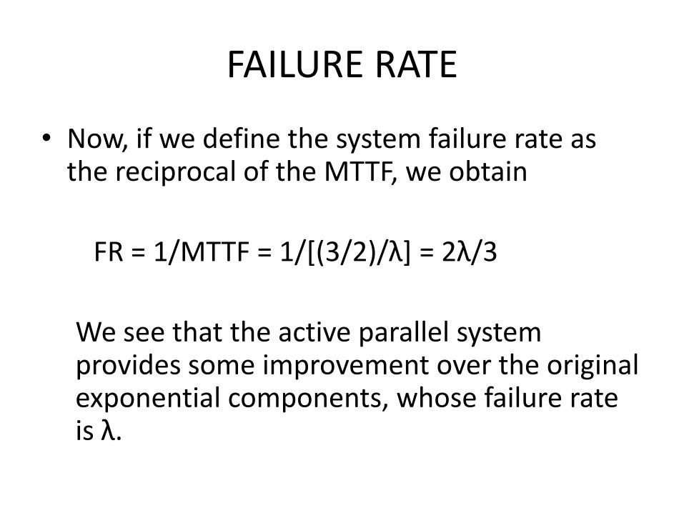
FAILURE RATE

• Now, if we define the system failure rate as the reciprocal of the MTTF, we obtain

FR = 1/MTTF = 1/[(3/2)/λ] = 2λ/3

We see that the active parallel system provides some improvement over the original exponential components, whose failure rate is λ.

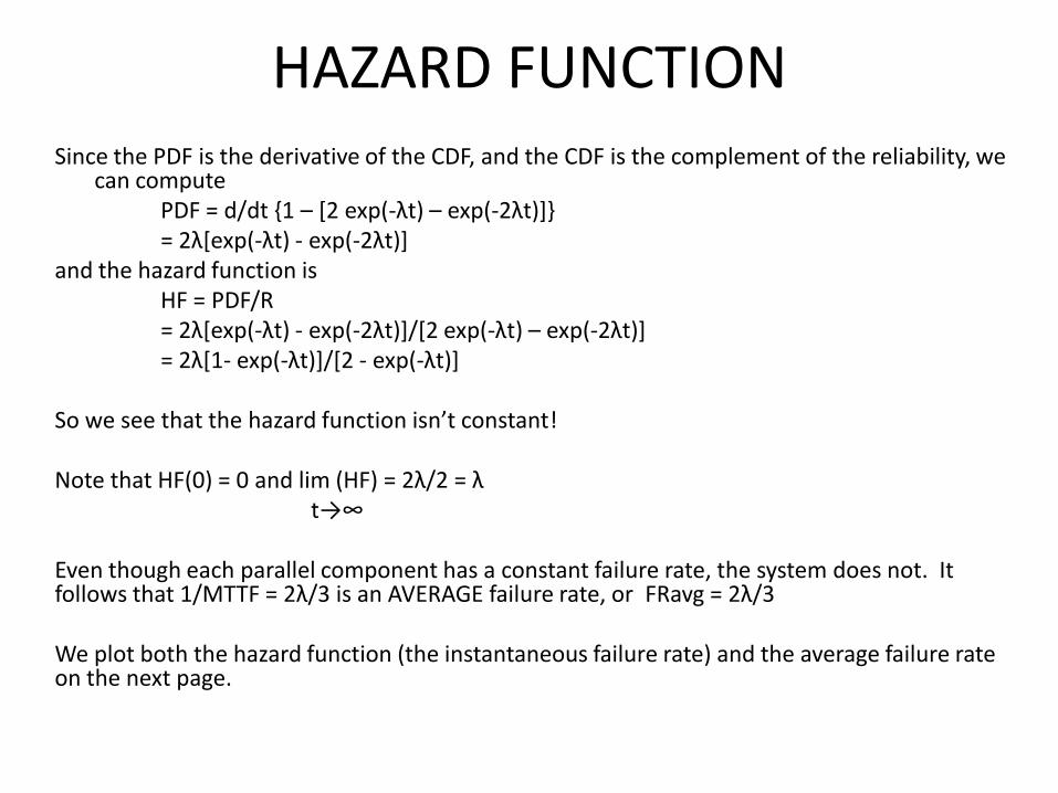
HAZARD FUNCTION Since the PDF is the derivative of the CDF, and the CDF is the complement of the reliability, we

can compute PDF = d/dt {1 – [2 exp(-λt) – exp(-2λt)]} = 2λ[exp(-λt) - exp(-2λt)] and the hazard function is HF = PDF/R = 2λ[exp(-λt) - exp(-2λt)]/[2 exp(-λt) – exp(-2λt)] = 2λ[1- exp(-λt)]/[2 - exp(-λt)] So we see that the hazard function isn’t constant! Note that HF(0) = 0 and lim (HF) = 2λ/2 = λ t→∞ Even though each parallel component has a constant failure rate, the system does not. It follows that 1/MTTF = 2λ/3 is an AVERAGE failure rate, or FRavg = 2λ/3 We plot both the hazard function (the instantaneous failure rate) and the average failure rate on the next page.

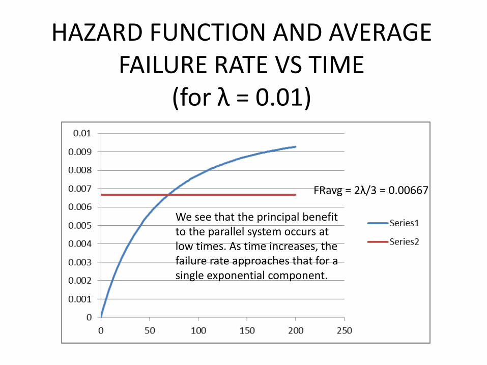
HAZARD FUNCTION AND AVERAGE FAILURE RATE VS TIME

(for λ = 0.01)

FRavg = 2λ/3 = 0.00667

We see that the principal benefit to the parallel system occurs at low times. As time increases, the failure rate approaches that for a single exponential component.

IRRESISTIBLE FORCE VS IMMOVABLE OBJECT The great reliability confrontation

• Irresistible Force: The more complex the system, the lower the system reliability and the more failures you will have.

• Immovable Object: If the reliability of your components is high enough, you will have few if any system failures.

• Intuitively, we might think that a goal of zero catastrophic mishaps over a fleet lifetime is realistic if the parts are reliable enough.

• To see how this plays out in a simple scenario, we examine the risk associated with operating a generic aircraft with many components, and try to predict how many system failures we might have over a typical fleet lifetime given high reliability parts.

• The risk associated with system operation is a function of the reliabilities of the critical safety items (CSI’s) of the components and subsystems.

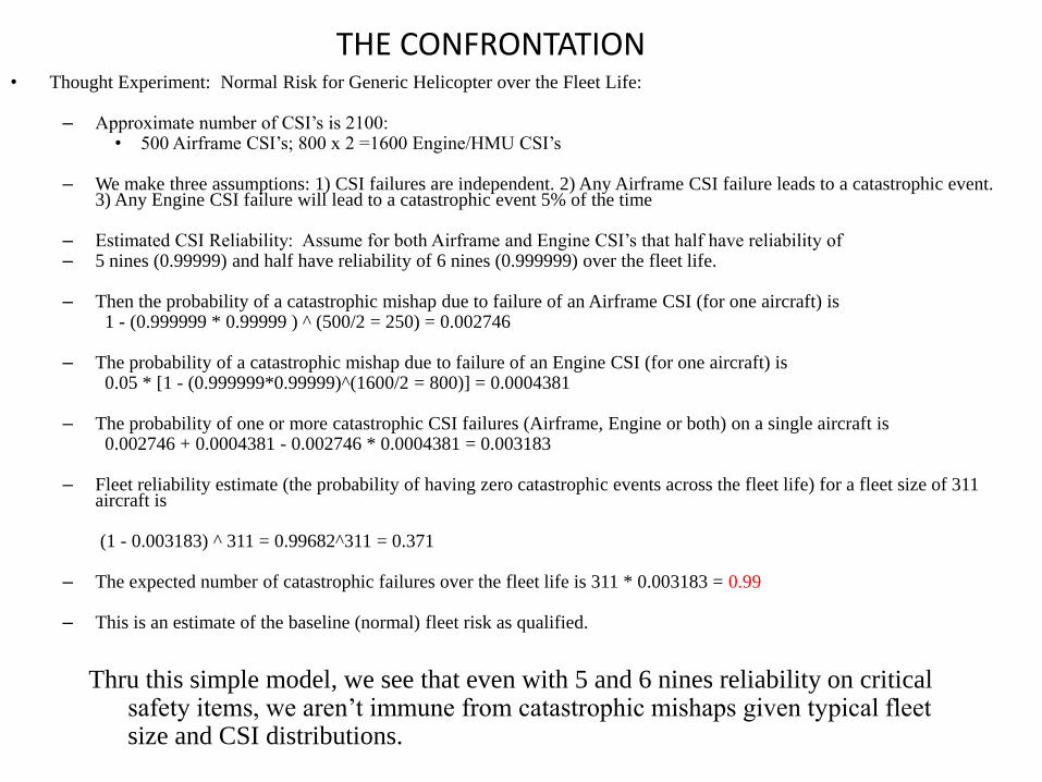
THE CONFRONTATION • Thought Experiment: Normal Risk for Generic Helicopter over the Fleet Life:

– Approximate number of CSI’s is 2100:

• 500 Airframe CSI’s; 800 x 2 =1600 Engine/HMU CSI’s

– We make three assumptions: 1) CSI failures are independent. 2) Any Airframe CSI failure leads to a catastrophic event. 3) Any Engine CSI failure will lead to a catastrophic event 5% of the time

– Estimated CSI Reliability: Assume for both Airframe and Engine CSI’s that half have reliability of – 5 nines (0.99999) and half have reliability of 6 nines (0.999999) over the fleet life.

– Then the probability of a catastrophic mishap due to failure of an Airframe CSI (for one aircraft) is 1 - (0.999999 * 0.99999 ) ^ (500/2 = 250) = 0.002746

– The probability of a catastrophic mishap due to failure of an Engine CSI (for one aircraft) is 0.05 * [1 - (0.999999*0.99999)^(1600/2 = 800)] = 0.0004381

– The probability of one or more catastrophic CSI failures (Airframe, Engine or both) on a single aircraft is 0.002746 + 0.0004381 - 0.002746 * 0.0004381 = 0.003183

– Fleet reliability estimate (the probability of having zero catastrophic events across the fleet life) for a fleet size of 311

aircraft is

(1 - 0.003183) ^ 311 = 0.99682^311 = 0.371

– The expected number of catastrophic failures over the fleet life is 311 * 0.003183 = 0.99

– This is an estimate of the baseline (normal) fleet risk as qualified.

Thru this simple model, we see that even with 5 and 6 nines reliability on critical safety items, we aren’t immune from catastrophic mishaps given typical fleet size and CSI distributions.

WEIBULL ANALYSIS OF LIFE-LIMITED PARTS

• Let’s say we have a population of fielded parts which have a life limit of T hours imposed due to a wearout mode.

• Once a part accumulates T hours, we replace it with a brand new part.

• All of our failure events have occurred before time T, and none of our unfailed parts have accumulated more than T hours.

• We want to lower the life limit to reduce the failure rate to a desired small value

• If we base the life limit on a straightforward Weibull analysis on this data, will the limit be acceptable, too conservative, or too optimistic?

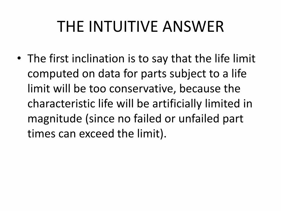
THE INTUITIVE ANSWER

• The first inclination is to say that the life limit computed on data for parts subject to a life limit will be too conservative, because the characteristic life will be artificially limited in magnitude (since no failed or unfailed part times can exceed the limit).

COMPLICATED TRUTH: IMPACT OF LIFE LIMIT ON WEIBULL RANK REGRESSION • Paul Barringer, P.E. (of Barringer and Associates, Inc.) sent me

two plots to illustrate that, in the case of rank regression, a Weibull analysis of fielded parts that are subjected to a life limit may or may not be conservative depending on how the failure times happen to line up with the true time-to-failure line for the population. These plots appear on the next two pages.

• The red data points are based on a random draw of 20 data points in SuperSMITH 5.0CL, and represent complete failure time data for a population of parts.

• The blue points represent the same data, but with a 5 year life limit instituted, thereby transforming failure times greater than 5 years into suspensions at 5 years.

CASE WHEN LIFE LIMIT DOES NOT AFFECT WEIBULL LINE

In this plot, (because the earliest two failures lie on/near the trendline for completely known data), the red and blue lines are virtually identical.

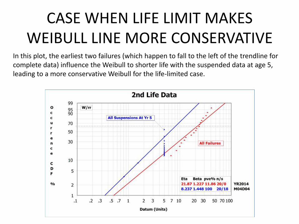
CASE WHEN LIFE LIMIT MAKES WEIBULL LINE MORE CONSERVATIVE

In this plot, the earliest two failures (which happen to fall to the left of the trendline for complete data) influence the Weibull to shorter life with the suspended data at age 5, leading to a more conservative Weibull for the life-limited case.

SAMPLE SIZE: EXTREME PRACTICES

• It is not unheard of that compliance with an engineering specification requirement is based on the outcome of a single pass/fail test

• On the other hand, if we become slaves to sample size formulas, we may create requirements that are unnecessary, unreasonable, and cost-prohibitive

SAMPLE SIZE FOR RELIABILITY DEMONSTRATION WITH ZERO

FAILURES (based on Clopper-Pearson)

• N = log(1 – C)/log R when R is the reliability we want to demonstrate with

confidence C

• So to demonstrate 90% reliability (r = 0.9) with 90% confidence (c = 0.9), we obtain N = 21.854… which rounds up to 22

• Similarly, to demonstrate 95% reliability with 95% confidence requires 58.40… or 59 successful tests without a failure, etc.

SAMPLE SIZE FOR BAYESIAN RELIABILITY DEMONSTRATION

• This approach is due to Dimitri Kececioglu*, a professor at Arizona State University in Tucson.

• Sample size can be computed based on – the required reliability, R – some initial degree of belief, P, that the reliability requirement has

been met.

• In this approach, the amount of initial degree of belief, or prior confidence (that is, human confidence, or “engineering judgment”), is used to determine the number of successful tests needed to demonstrate the desired reliability with any desired confidence.

* Note: I am sorry to report that Dimitri Kececioglu passed away on March 21, 2014, at the age of 91.

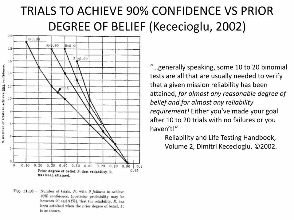
TRIALS TO ACHIEVE 90% CONFIDENCE VS PRIOR DEGREE OF BELIEF (Kececioglu, 2002)

“…generally speaking, some 10 to 20 binomial tests are all that are usually needed to verify that a given mission reliability has been attained, for almost any reasonable degree of belief and for almost any reliability requirement! Either you’ve made your goal after 10 to 20 trials with no failures or you haven’t!”

Reliability and Life Testing Handbook, Volume 2, Dimitri Kececioglu, ©2002.

FINAL THOUGHTS

We have seen that our intuition may betray us even when facing relatively simple reliability problems. But intuition trained by experience is a formidable asset. "Intuition isn't the enemy but the ally of reason." John Kord Lagemann

QUESTIONS?

• Jim Bartlett, ASQ CRE

– Email james.k.bartlett.civ@mail.mil

– Phone COM (256)313-9075, DSN 897-9075