Reliability Analysis with Suspended Items

submitted by

Harold John Gregory BARTLETT B.E.(Hons) B.Sc.(Hons)

of the

School of Mechanical, Manufacturing and Medical Engineering Queensland University of Technology

pursuant to the requirements for the award of the degree of

Doctor of Philosophy (Ph.D.)

February 1998

QUT

QUEENSLAND UNIVERSITY OF TECHNOLOGY DOCTOR OF PHILOSOPHY THESIS EXAMINATION

CANDIDATE NAME

CENTRE/RESEARCH CONCENTRATION

PRINCIPAL SUPERVISOR

ASSOCIATE SUPERVISOR(S)

Harold Bartlett

Tribology

Prof Nick Hastings

Prof Anthony Pettitt Mr Len Bradshaw

THESIS TITLE Reliability Analysis with Suspended Items

OV\ ~ '& N ~" I ot q7 Under the requirements of PhD regulation 9.2, the above candidate was examined orally by the Faculty. The members of the panel set up for this examination recommend that the thesis be accepted by the University and forwarded to the appointed Committee for examination.

ff\o 1~ . N , A. T (~ A-J'It N J,j . Name ...................................................... :-:- ........ Slgnature

Panel Chairperson (Principal Supervisor)

Name.~~ -~:~;·/1~~{~ .............. Signature

])r-. 12. M A\--\ A C... I NGA -'"llFR.. . Name ............................... . ... . ............................ S1gnaturePanel Member

Name ..... P./!;9..F.. .... ~ ..... ~0..IT .. ................. SignaturePanel Member

Under the requirements of PhD regulation 9.15, it is hereby certified that the thesis of the above-named candidate has been examined. I recommend on behalf of the Thesis Examination Committee that the thesis be accepted in fulfilment of the conditions for the award of the degree of Doctor of Philosophy.

Name~· . ??.0 . .f.(A:~.C[:~ ql__l(~ Signature Date .. . f.:.7. ~- .'f..f.. .... Chair of Examiners (External Thesis Examinati

QUT Verified Signature

QUT Verified Signature

QUT Verified Signature

QUT Verified Signature

QUT Verified Signature

Keywords : reliability analysis, reliability estimation, probability distribution,

distribution fitting, censored samples, multiple censoring, censored

item, suspension, suspended item, graphical methods.

Abstract

Reliability analysis has several important engineering applications. Designers and

operators of equipment are often interested in the probability of the equipment

operating successfully to a given age - this probability is known as the

equipment's reliability at that age. Reliability information is also important to

those charged with maintaining an item of equipment, as it enables them to model

and evaluate alternative maintenance policies for the equipment.

In each case, information on failures and survivals of a typical sample of items is

used to estimate the required probabilities as a function of the item's age, this

process being one of many applications of the statistical techniques known as

distribution fitting.

In most engineering applications, the estimation procedure must deal with

samples containing survivors (suspensions or censorings); this thesis focuses on

several graphical estimation methods that are widely used for analysing such

samples. Although these methods have been current for many years, they share a

common shortcoming: none of them is continuously sensitive to changes in the

ages of the suspensions, and we show that the resulting reliability estimates are

therefore more pessimistic than necessary. We use a simple example to show that

the existing graphical methods take no account of any service recorded by

suspensions beyond their respective previous failures, and that this behaviour is

inconsistent with one's intuitive expectations.

In the course of this thesis, we demonstrate that the existing methods are only

justified under restricted conditions. We present several improved methods and

demonstrate that each of them overcomes the problem described above, while

reducing to one of the existing methods where this is justified. Each of the

improved methods thus provides a realistic set of reliability estimates for general

(unrestricted) censored samples. Several related variations on these improved

methods are also presented and justified.

- i -

Table of Contents

Front Matter

Keywords .................................... .

Abstract ..................................... .

Table of Contents . . . . . . . . . . . . . . . . . . . . . . . . . . . . . . . . . n

List of Illustrations . . . . . . . . . . . . . . . . . . . . . . . . . . . . . . . . vi

List of Tables ................................... vii

Notation . . . . . . . . . . . . . . . . . . . . . . . . . . . . . . . . . . . . . viii

Dedication . . . . . . . . . . . . . . . . . . . . . . . . . . . . . . . . . . . . xm

Acknowledgements . . . . . . . . . . . . . . . . . . . . . . . . . . . . . . . xiii

Statement of Originality . . . . . . . . . . . . . . . . . . . . . . . . . . . . xiii

Chapter 1: Introduction, Background and Outline

1. 0 Introduction . . . . . . . . . . . . . . . . . . . . . . . . . . . . . . . . . 1

1.1 Background . . . . . . . . . . . . . . . . . . . . . . . . . . . . . . . . . 1

1.1.1 Maintenance 1

1.1.2 Modelling and optimising maintenance 2

1.1.3 Reliability analysis 2

1.2 Outline of Thesis . . . . . . . . . . . . . . . . . . . . . . . . . . . . . 3

Chapter 2: Review of Reliability Estimation Methods

2.0 Introduction . . . . . . . . . . . . . . . . . . . . . . . . . . . . . . . . . 5

2.1 Definitions and Terminology . . . . . . . . . . . . . . . . . . . . . . 5

2.2 Maximum Likelihood Estimation Methods . . . . . . . . . . . . . . 7

2.3 Graphical Methods for Complete Samples . . . . . . . . . . . . . . 8

2.3.1 Step-function plots of reliability

2.3.2 Point estimates of reliability

2.3.3 Effects of sample size

2.4 Singly and Multiply Censored Samples

2.4.1 Kaplan-Meier estimates

2.4.2 Herd and Johnson methods

2.4.3 Cumulative hazard plots

2.4.4 Effects of sample size

- ii -

9

10

11

11

12

13

15

16

2.5 Limitations of Existing Graphical Methods . . . . . . . . . . . . . 16

2. 6 Currency of Existing Methods . . . . . . . . . . . . . . . . . . . . 18

2.7 Summary . . . . . . . . . . . . . . . . . . . . . . . . . . . . . . . . . 18

Chapter 3: A Continuous Generalisation of the Herd-Johnson Formula

3.0 Introduction . . . . . . . . . . . . . . . . . . . . . . . . . . . . . . . . 19

3 .1 Motivation for Generalisation . . . . . . . . . . . . . . . . . . . . . 19

3.2 Derivation of Improved Reliability Estimates . . . . . . . . . . . 22

3.2.1 The improved estimates 22

3.2.2 Derivation of estimates 23

3. 3 Properties of the Improved Estimates . . . . . . . . . . . . . . . . 23

3.4 Simplified Form for Grouped Suspensions . . . . . . . . . . . . . 25

3.5 Treating "Simultaneous" Failures . . . . . . . . . . . . . . . . . . . 25

3.6 Examples . . . . . . . . . . . . . . . . . . . . . . . . . . . . . . . . . 27

3.6.1 Numerical example 27

3.6.2 Theoretical example 28

3. 7 Formulation in Terms of Modified Order Numbers . . . . . . . . 29

3. 8 Summary . . . . . . . . . . . . . . . . . . . . . . . . . . . . . . . . . 30

Chapter 4: An Improved Variant of the "Hazard Plotting" Method

4.0 Introduction . . . . . . . . . . . . . . . . . . . . . . . . . . . . . . . . 31

4.1 Deriving the Improved Hazard Plotting Method 31

4 .1.1 Motivation for changes 31

4.1.2 Improved estimates for cumulative hazard values 32

4.1.3 Multiple suspensions and "multiple" failures 33

4.2 Properties of the Improved Estimates . . . . . . . . . . . . . . . . 34

4.3 Worked Example . . . . . . . . . . . . . . . . . . . . . . . . . . . . 35

4.4 Summary . . . . . . . . . . . . . . . . . . . . . . . . . . . . . . . . . 36

Chapter 5: Better Estimates for Modified Order Numbers

5.0 Introduction . . . . . . . . . . . . . . . . . . . . . . . . . . . . . . . . 38

5.1 Modified Order Numbers and "Notional Failures" . . . . . . . . 38

5 .1.1 General discussion 38

5 .1. 2 Johnson's assumption 3 9

- iii -

5.2 Johnson's Estimate for the Notional Failures

5. 2.1 Deriving the estimates

40

42

45

46

5.2.2 Evaluating the estimates

5. 3 An Improved Estimation Method

5.4 An Alternative Improvement - the Second Stage Method . . . . 47

5.4.1 Derivation and formula 47

5.4.2 A simplified formula for computations 48

5.4.3 Properties of the improved estimates 48

5.5 Numerical Examples . . . . . . . . . . . . . . . . . . . . . . . . . . 49

5.5 .1 Example 1 - refining an initial estimate 50

5.5.2 Example 2 - demonstration of continuity 53

5.6 Summary .... : . . . . . . . . . . . . . . . . . . . . . . . . . . . . 55

Chapter 6: Various Extensions of Earlier Results

6.0 Introduction . . . . . . . . . . . . . . . . . . . . . . . . . . . . . . . . 56

6.1 Non-Parametric Reliability Estimation ......... .

6.1.1 Description of method

6.1.2 Worked examples

6.1.3 Properties of the estimate

57

57

58

60

6.2 Extending Reliability Estimates Beyond the Final Failure 61

6.2.1 Limitations of current graphical methods 62

6.2.2 Optimistic and pessimistic envelopes 63

6.2.3 The "next failure" estimates 64

6.2.4 A numerical example 65

6.2.5 Validity and significance of the "next failure" estimates 66

6.2.6 Other comments 67

6.2. 7 Connection to earlier chapters 68

6.3 Conversion to Median Ranks and/or Other Estimates

6.3.1 Large samples with few suspensions

68

69

6.3.2 Small multiply-censored samples 70

6.4 Step Function Reliability Estimates . . . . . . . . . . . . . . . . . . 74

6.4.1 Direct modification of the Kaplan-Meier estimate 74

6.4.2 A further alternative for step function estimates 75

- iv -

6.5 Summary . . . . . . . . . . . . . . . . . . . . . . . . . . . . . . . . . 77

Chapter 7: Summary. Discussion. Suggestions and Conclusions

7.0 Precis . . . . . . . . . . . . . . . . . . . . . . . . . . . . . . . . . . . 78

7.1 Summary of Thesis Content . . . . . . . . . . . . . . . . . . . . . . 78

7 .1.1 Review of existing methods 7 8

7.1.2 Improved graphical methods 78

7 .1. 3 Further improvements and extensions 79

7.2 Significance and Applicability of the Ideas and Methods Presented . . . . . . . . . . . . . . . . . . . . . . . . . . . . . . . . 80

7.3 Suggestions for Further Work . . . . . . . . . . . . . . . . . . . . . 81

7. 3.1 Evaluating the impact of these results 81

7.3.2 Dealing with dependent suspensions 82

7.3.3 Application to goodness-of-fit testing

7.4 Conclusions . . . . . . .................... .

7.4.1 Improved reliability estimates

7.4.2 Extended reliability estimates

7.4.3 Further possibilities

Bibliography

References cited

Publications based on the work described in this thesis . . . . . ....

- v -

82

83

83

84

84

85

86

List of Illustrations

Chapter 2:

Figure 2.1 - Reliability Plots for Complete Samples 8 (a) edf estimate (b) midpoint estimates (c) mean rank estimates (d) median rank estimates

Figure 2.2 - Reliability Plots for Multiply Censored Samples 13 (a) Kaplan-Meier estimate (b) Herd I Johnson estimates (c) Cumulative hazard estimates

Figure 2.3 - Reliability Plots for Example Data 18 (a) Cases 1, 2, 3 (b) Case 4

Chapter 3:

Figure 3.1 - Graphical Representations of Herd's Formula 20 (a) censored (b) uncensored

Figure 3.2 - Graphical Representation for Suspensions Mid-Interval 22

Figure 3.3 - Reliability Plots of Example Data 28

Figure 3.4 - Theoretical Comparison: Improved Method vs Herd-Johnson 29

Chapter 4:

Figure 4.1 - Numbers at Risk vs Age for Various Samples 32

Figure 4.2 - Reliability Plot of Example Estimates 35

Chapter 5:

Figure 5.1 - Graphical Representation of Johnson's Modified Order

Numbers (a) mi vs i (b) mt vs ki* 41

Figure 5.2 - Combined Representaion of Previous Figure 43

Figure 5.3 - Graphical Representations: Further Example 44

Figure 5.4 - Graphical Representation for Suspensions Mid-Interval 46

Figure 5.5 - Weibull Reliability Plot for Example Data 51

Figure 5.6 - Linear Reliability Plot for Example Data 52

Figure 5.7 - Weibull Reliability Plot: Second Example 53

Figure 5. 8 - Linear Reliability Plot: Second Example 54

Chapter 6:

Figure 6.1 - Graphical Representation for Suspensions Mid-Interval 57

Figure 6.2 - Non-Parametric Estimate for Johnson's Example Data 59

Figure 6.3 - Non-Parametric Estimate for Simulated Example Data 60

Figure 6.4 - Extended Kaplan-Meier Reliability Estimates 63

Figure 6.5 - Extended "Chapter 3" Reliability Estimates 64

Figure 6.6 - Reliability Plots with Confidence Bands: O'Connor's Data 71 (a) "fixed" sample size (b) "reducing" sample size

Figure 6. 7 - Modified Kaplan-Meier Reliability Plot 75

Figure 6.8 - "Sloping Step-Function" Reliability Plot 77

- vi -

List of Tables

Chapter 2:

Table 2.1 Example Reliability Data 17

Table 2.2 Reliability Estimates from Example Data 17

Chapter 3:

Table 3.1 Variations of Johnson's Example Data 27

Table 3.2 Reliability Estimates by Case and Estimation Method. 27

Chapter 4:

Table 4.1 Example Reliability Data 36

Table 4.2 Comparative Estimates from Example Data 36

Chapter 5:

Table 5.1 Example Analysis (Johnson's Data) 50

Table 5.2 Calculation of Second Stage Estimates 51

Table 5.3 Calculation of Second Stage Estimates 52

Table 5.4 Example Reliability Data 54

Table 5.5 Second Stage Reliability Estimates CRi) for Multiple Cases 54

Chapter 6:

Table 6.1 Application of Method to Johnson's Example Data 59

Table 6.2 Application of Method to Simulated Example Data 60

Table 6.3 Failure Data and Reliability Estimates 65

Table 6.4 Example Data from O'Connor 69

Table 6.5 Reliability Estimates for Above Example 70

Table 6.6 Modified Reliability Estimates for Above Example 73

Table 6.7 Continuously Sensitive Alternative to Kaplan-Meier Method 75

Table 6.8 - Calculations for Sloping Step-Function Example 76

- vii -

Notation

Symbol Description

1. Sample Data

A number (n) of identical items is placed in service. For each item, the age is

recorded at which that item fails; if it does not fail, the latest age is recorded at

which it was known to be in service1• These ages are then ordered from smallest

to largest.

n Sample size = number of items placed on trial

k index for ordered list of (all) ages

E Event (failure or suspension)

s Suspension = item other than failure

Ek k-th event; also, age at k-th event

i Order number = index for ordered list of failures

!; i-th failure; also, age at i-th failure

j index for ordered list of suspensions

sj j-th suspension; also, age at j-th suspension

ki indicates that event Ek is a failure event (viz.!;): ki is the event

index (k) corresponding to the order number i

~ indicates that event Ek is a suspension (viz. s): kj is the event

index (k) corresponding to the suspension index j

J index for ordered list of groups of suspensions (each group consists

of items suspended at the same age)

N1 number of items in J-th group of suspensions

k1 event index (k) corresponding to the first item in the J-th group of

suspensions

1. This could be the age at which it was removed from service (due to completion of the trial or for other reasons) or its age when analysis commenced (if the item was still in service then).

- viii -

2. (Probability) Distribution of Failure Ages

One of the aims of reliability analysis is to fit a theoretical distribution to the

sample data on ages at failure or suspension. This distribution aims to describe

typical failure I survival behaviour of the items under consideration, and is often

used for further analysis, eg. in optimising a maintenance policy model for such

items. Several representations of such a distribution are described below, any one

of which uniquely determines each of the others: in other words, they each

contain equivalent information about the distribution concerned.

t Age of typical item

R(t) Reliability (survivor) function = Prob (item survives beyond age t)

F(t) (cumulative) Distribution function (edt) = 1 - R(t)

= Prob (item fails at or before age t)

f(t) probability density function (pdf) = dF ldt

= (absolute) "rate" of failures at age t

z(t) hazard rate (function? = f(t) I R(t) = "rate" of failure at age t

conditional on survival until that age

H(t) cumulative hazard rate (function) = S~ z(s) ds = - ln(R(t))

We also use obvious extensions of the above notation, eg. when discussing an

event E (which occurs at age t =E), we will commonly use R(E) instead of R(t).

In addition, the standard notation for conditional probability:

Prob(A I B) probability of event A occurring, given that event B occurs (ie.

conditional on the occurrence of event B )

is adapted as follows:

R(E'IE) Prob (survival to age E') conditional on survival to ageE

2. We avoid using the term "failure rate", as some authors use it to mean the pdf Cf(t) ), while others use it to denote the hazard rate function (z(t) ).

- ix -

3. Quantities Calculated from Sample Data

i*, j*, k* "reverse" indices: n + 1 - i, n + 1 - j, n + 1- k

R(t), Ri estimated (sample) reliability: at age t, at ageh

mi modified order number of failure h

mt "reverse" modified order number = n + 1 - mi

H(t), Hi estimated cumulative hazard: at age t, at ageh

ilHi cumulative hazard (estimate) increment = Hi - Hi_ 1

Mi (or M) (for a given failure h) according to context, the largest value of the

suspension indexj (suspension group index J) such that sj <h (s1 <h); the subscript i may be omitted when the meaning is clear.

aj proportion of interval (between failures) survived by suspension sj

= (sj - h-1) I (h - h-1) (where3 h-1 ~ sj < h)

a1 common value of af for items in the J-th group of suspensions

(3j for suspension sj, proportion of interval (between failures)

occupied by sub-interval since the previous event (EP say)

= (sj - EP) I (h - h-1) (where3 h-1 ~ sj < h);

= a. -a. 1 if E =s. 1 1 ;- p J-

(3i for failure h, proportion of interval (between failures) occupied by

sub-interval since the previous event (EP say)

= (h-EP )lf..h-h-1 ); = 1 if EP =h-1, = 1-aj if EP =sj_1

a; = aj if EP is a suspension sj ; = 0 if EP is a failure h

Ai modification (adjustment) in i-th order number = mi - i

pij (estimated) probability of surviving item at age sj failing at or

before ageh

3. (If required, define fo = 0 for consistency.)

- X -

r if (estimated) probability of surviving item at age sj continuing to

survive beyond age h = 1 - pif

~(or I)

RP (t), R{,

R~ J

(for a given suspension sj) the smallest order number i such that

sj <h ; the subscript j may be omitted when the meaning is clear.

fitted (parametric) reliability estimate: at age t, at age h, at age sj

ni notional sample size at failure h = original sample size n

adjusted for the existence and ages of any suspensions occurring

beforeh

4. Miscellaneous

E summation of terms over the given range of the index; by

convention, an empty sum takes the value of zero (0).

ll product of terms over the given range of the index; by convention,

an empty product takes the value of unity (ie, 1).

s- statistical(ly): used to highlight the use of technical statistical terms

such as (s-)expected values, (s-)independent variables, etc.

[a, b) a half-open interval: the set of values t such that a < t < b.

LHS left hand side

- xi -

to my God, with love;

also, in memory of my father.

Thanks and Acknowledgements

I wish to acknowledge with thanks the help and support given by my wife Helen

and my children during my Ph.D. candidacy. Thanks also to my Ph.D.

supervisors and to the many other family members, colleagues and friends who

have helped and supported me through these testing times.

The work described in this thesis was partly supported by a scholarship from

MIM Holdings Limited, and by an Australian Post-Graduate Research Award

scholarship, both of which are also gratefully acknowledged.

Statement of Originality

The work contained in this thesis has not been previously submitted for a degree

or diploma at any other higher education institution. To the best of my knowledge

and belief, the thesis contains no material previously published or written by

another person except where due reference is made.

(signed) (date)

- xiii -

QUT Verified Signature

Chapter 1 : Introduction. Background and Outline

1. 0 Introduction

The task of managing maintenance activities and requirements is a complex and

multi-faceted one, but primarily dedicated to the responsibility of ensuring that

the equipment required is available (in working condition) at the required times at

the lowest feasible cost. Among the resources available to assist in this task, the

methods of maintenance modelling and optimisation provide theoretical tools for

guiding practical policies and decisions. In this thesis we discuss a particular

aspect of maintenance modelling, with a view to increasing the accuracy of the

information that it provides to the overall process of maintenance management.

The particular aspect we concentrate on is the estimation of item reliability from

typical performance data (viz. operating times to failure, to other replacement, or

to current non-failure). The resulting reliability estimates not only are useful for

their own sake, but also provide necessary information for modelling and

optimising appropriate maintenance policies, which may in turn help to lower

overall maintenance costs.

The general setting of our work is described more fully in the next section,

followed by an overview of the substantive chapters to follow.

1.1 Background

1.1.1 Maintenance

Every human endeavour involves the use of tools or equipment of some sort, and

it is a universal observation that these tools and equipment eventually deteriorate

and wear out. In some situations, a complete replacement of the spent item is

appropriate, while in others the replacement or repair of certain parts of the

equipment is more economical. The timing of any remedial actions can also be

important: in some cases these actions are undertaken once the equipment has

ceased being useable, and in other cases it may be better to perform them earlier

in an attempt to forestall the deterioration. In many cases, a combination of these

approaches may be more desirable than any single alternative.

- 2 -

Such considerations are the essence of maintenance work, which may be defined

as the responsibility for ensuring that suitable equipment is available in suitable

condition to perform a given task on an ongoing basis.

1.1.2 Modelling and optimising maintenance

In most settings (both commercial and non-commercial), those responsible for

managing the maintenance of equipment also have an inherent responsibility to

use their resources (time, money, personnel, etc.) efficiently: as a result, they

will be seeking to find and use those repair I replacement approaches which are

the most economical in overall terms among the approaches available to them.

The ability to analyse and compare the likely costs (and other outcomes) of

different maintenance approaches will therefore be an important aid to the

successful fulfilment of these responsibilities. The field of maintenance modelling

seeks to carry out such analyses, and is the broader background in which the

work of this thesis is set.

1.1.3 Reliability analysis

In order to model the effects of various maintenance policies for a given type of

equipment, it is necessary to know the likely costs and proposed frequencies of

various maintenance actions, together with the likely cost and frequency of

component or equipment failure. In most cases the required costs can be

estimated fairly confidently and the proposed frequency of maintenance is

determined by the analysis itself, while a realistic description of the equipment's

failure behaviour generally involves the concept of a probability distribution for

each component's age at failure. The use of such a distribution allows for the

variations which occur between the failure ages of apparently identical

components in apparently identical situations.

Just as the estimated cost figures are based on current and historical knowledge of

the items and procedures concerned, the estimated distributions of failure ages are

based on historical performance records of the components concerned. The

estimated distributions are then used to help predict the likely outcome (in a long­

term average sense) of applying the various maintenance policies proposed.

- 3 -

Although we have introduced the estimation of failure distributions as a necessary

part of the maintenance modelling process, these distributions also have direct

applications of their own. In particular, designers and operators of equipment are

often interested in the probability of the equipment operating successfully to a

given age - this probability is the complement of the failure probability, and is

known as the equipment's reliability. Such information is particularly useful to

designers and operators of limited-term or strategically critical equipment. Due to

the prevalence of such applications, the estimation of failure distributions is

commonly known as "reliability analysis" in both design and maintenance circles.

The theoretical basis for distribution-fitting techniques belongs to the field of

statistical analysis. The estimation of failure distributions from data on equipment

performance is only one of the practical applications for these techniques. Other

applications include actuarial considerations, medical research, hydrological

analysis, and various other analyses that model recurrent but variable behaviour.

In some of these fields, the term "survival analysis" is more commonly used.

1.2 Outline of Thesis

We have discussed the basic aims of reliability estimation in the previous section.

In Chapter 2, we describe the procedures used to estimate the relevant failure age

distributions, including those procedures generally used in engineering

applications. We assume that the reader has a working knowledge of the

terminology and concepts associated with probability distributions: page viii of

the Notation section gives a brief summary of the notation we will use in this

regard.

In most engineering applications, the estimation procedure must deal with

samples in which not all of the items have failed, and our descriptions focus on

certain graphical estimation methods that are widely used for analysing such

samples. Although these methods have been current for many years, they all

share a common shortcoming, which is that none of these methods IS

continuously sensitive to changes in the ages of the unfailed items; we

demonstrate this shortcoming by use of a simple example.

- 4 -

Chapters 3 to 6 present and discuss several improvements to the current methods

that were described in Chapter 2. The methods of Chapters 3, 4 and 5 extend and

correct the current methods due to Herd, Nelson and Johnson respectively1,

while Chapter 6 discusses several other proposals and developments related to the

methods of Chapters 3 to 5.

In all cases, the improved methods we present overcome the shortcoming of the

existing methods by being fully sensitive to changes in the ages of unfailed items.

The results of the improved analysis methods should therefore be more accurate

than those of the existing methods. The improvement in accuracy of these

methods is most noticeable in situations where the number of failures is small and

the number of unfailed items is large.

Chapter 7 provides a summary of the results presented in the previous chapters,

together with a discussion of the significance and applicability of our work, some

suggested topics for further research, and some brief conclusions. Additional

material following this concluding chapter comprises a bibliography of the

references cited in this thesis, a list of published papers related to the work

described in this thesis, and a copy of each of the latter.

1. Relevant bibliographic references are given in Chapter 2 and ff.

Chapter 2: Review of Reliability Estimation Methods

2.0 Introduction

Practitioners in many fields are interested in the survival characteristics of

various items, eg. organisms or equipment. This information is usually presented

in terms of the item's reliability or survivor function: that is, the (estimated)

probability of one such item functioning properly until (at least) a given age. The

engineering applications of such information include modelling of alternative

maintenance policies, as well as reliability determination per se.

We discuss below various methods for estimating the reliability function for a

given item of equipment from its available lifetime I performance data.

2.1 Definitions and Terminology1

Reliability trials commonly produce some items which have failed and some

which have not (yet) failed, the latter being known as suspensions (also,

suspended items) or censorings (also, censored items)2•

3• A data set which

contains such censorings is known as a censored sample : when all suspensions

outlast all failures, the sample is singly censored; when some suspensions pre­

date some failures, the sample is multiply censored. A data set in which all items

fail (ie, none are suspended) is called a complete sample.

In analysing a data set, the failures and suspensions are first ordered into separate

lists by age. We use the symbols h and sj to denote the i-th failure and the j-th

suspension in their respective lists; the index i is commonly referred to as the

order number of the failure h· We also sort the two lists together into a combined

list of events and use Ek to denote the k-th event in this list. (An event is either a

1. See also list of Notation, p vii.

2. These terms apply to any items removed from trial I service before failure, as well as those still in service at the time of data collection.

3. Strictly, the suspensions we consider here are known as right censorings. Other forms of censoring (left censoring, double censoring) are also possible, but are rarely encountered in the maintenance I reliability field. They can usually be dealt with by fairly straightforward adaptation or extension of the methods described here.

- 6 -

suspension or a failure.) If any of the suspensions is simultaneous with a failure,

the common convention is to list the failure first in the combined list, ie. to treat

the suspension(s) as occurring immediately after the failure.

If the event Ek is a failure h we may also write k as ki ; similarly, if Ek is a

suspension sj , we may write k as Js . The abbreviated notation k* will be used to

denote the number n + 1 - k, with similar definitions for i*, kt , etc.

For notational brevity, we shall also use h (etc.) to represent the age at which the

corresponding event occurred. Depending on the equipment and operation

concerned, this may be measured in calendar time, operating time, operating

cycles, distance travelled, etc, the obvious restriction being that the same

measurement units must be used for all the items in a given data set. We also

assume that the operating I trial conditions are independent of calendar time, in

which case the relative time origins of different sample items are irrelevant to our

discussions.

As noted above, the analyst's atm is to estimate an item's reliability function

from the recorded ages of both failed and suspended items. Most commonly, a

particular family of shapes (a parametric form) for the reliability function is

assumed before the analysis is done: in maintenance modelling applications,

distributional forms such as the Weibull, log-Normal, Normal and Gamma

distributions are most commonly used. The mathematical definitions of these can

be found in many common text-books on reliability, such as [1] and [2].

Although less common in maintenance modelling applications, non-parametric

estimates of the reliability function may also be made.

Methods for obtaining parametric reliability estimates fall into two main groups,

viz. graphically based methods4 and maximum likelihood methods (also known as

generalised linear models). Non-parametric estimates are closely associated with

the former group, and so are often presented and treated as graphical estimates.

4. We use this term here to include also analytical methods based on essentially graphical reasoning, eg. linear regression of estimated probability levels against age. For brevity, we shall often refer to all such methods as graphical methods.

- 7 -

The graphical methods are generally preferred by maintenance and reliability

practitioners over the more formal maximum likelihood approach. Reasons for

this include the ability to gain a visual impression of the sample data before

commencing a formal analysis, and the related ability to try several different

distribution forms and see which forms fit the data best. It is also worth noting

that many maximum likelihood analyses are guided in practice by an initial

graphical analysis. For these reasons, and because of their widespread use, we

will concentrate our attention on graphical methods and provide only a brief

description of maximum likelihood methods.

2.2 Maximum Likelihood Estimation Methods

The application of maximum likelihood methods to reliability estimation is

described by Nelson at some length [2 ch 8], including example applications to

several common distributional forms. The essence of the method is to find the

specific distribution within a given distributional form which maximises the

probability of obtaining the sample results that were actually observed, ie. to find

values for the unspecified parameters of the distribution that will achieve this

objective. The required values will depend on the observed ages at failures and

suspensions, and are found by solving certain optimisation equations.

In general terms, the analysis follows the following lines. Whatever the failure

distribution, the probability of observing a failure at age h is proportional to the

probability density function at that age. Similarly, the probability of observing a

suspension at age si is given by the item's probability of surviving until this

observed age, that is, by its reliability function at the age si. The overall

probability of obtaining the sample observed is therefore proportional to the

product of these terms over all values of i and j. Given the assumed form of the

distribution, this product can be expressed as a function of the unknown

distribution parameters and of the known ages at failures and suspensions; the

optimisation equations are then obtained from this expression by using relatively

simple calculus and algebra. Solving these equations for the given data values5

5. For some distributions, the equations can be solved analytically before substituting the data values, but for most distributions they must be solved

- 8 -

then yields the desired parameter estimates.

Nelson [ibid] derives and presents the relevant equations for the exponential,

Normal and log-Normal, Weibull and Extreme Value distributions; he also gives

further references for dealing with generalised forms of these distributions.

Figure 2.1 - Reliability Plots for Complete Samples

2.3 Graphical Methods for Complete Samples

We concentrate in this thesis on the initial plotting aspects of the graphically

based methods, as these are also basic to any analytical variations that may be

added. The initial plot takes the form of either a series of steps or a series of

numerically. An alternative to the latter is to directly maximise the previous expression, by numerical methods.

- 9 -

representative points, one at each observed failure age (see Figure 2.1). As well

as providing an initial estimate of the item's reliability function6, this plot also

provides the basis for fitting a smooth (ie, continuous) reliability estimate to the

observed data - either "by hand" or using a suitable analytical I numerical

technique. A third use, which we shall not pursue further here, is to act as a

gauge for comparing the fit of any proposed distribution form.

It is only at the stage of fitting a smooth reliability estimate that the issue of

parametric vs non-parametric estimates affects the procedure used. Up to this

point, the reliability estimates obtained - whether in "step" or "point" form -

are essentially independent of any distributional assumptions; in fitting a

functional form to the reliability estimates, however, one must choose whether to

favour any particular family of shapes ("distributional form") over other possible

contenders. To obtain non-parametric estimates (not favouring any particular

family of shapes), the plot is usually done with linear scales on the axes, and the

smoothed estimate then takes the form of a non-linear curve. As an alternative,

and essentially implying a parametric form for the reliability estimate, the plot is

done with suitably transformed scales, chosen in a way which should yield a

"straight line" plot if a certain distributional form applies [eg. 3 p 24; 2 pp 107,

108, 125; 4 p 463]. The "straightness" of the sample plot then provides a

qualitative test for the applicability of the distributional form chosen.

2. 3.1 Step-function plots of reliability

The most basic probability plot for a complete sample is that of the empirical

distribution function (edtY [3 p 8; 2 p 106] which assigns an equal lump of

probability to each observed failure event. In terms of reliability, the plot for a

complete sample of size n is simply a step function which falls by an amount of

6. Some authors prefer to work in terms of estimating the distribution function (edt). Since this is just the complement of the reliability function, the differences involved in doing so are only minor matters of detail.

7. also known as empirical cdf or sample cdf; the term empirical refers to the fact that this estimate is based on the observed sample data, and not on any predetermined distributional form.

- 10 -

lin at each failure event (see Figure 2.1a); the corresponding formula is:

R(t) = (n-i)ln = (i*-1)/n, (2.1)

where i is determined by h_ s t < h+t.

In most cases, the edf is plotted on linear scales (thereby treating it as a non­

parametric estimate); however, there is no practical restriction which would

prevent the use of transformed (non-linear) scales.

Although one usually assumes the underlying distribution to be continuous rather

than stepped, the step-function form has some distinctive visual benefits: it

readily indicates the discrete nature of the observed sample, and it provides a

useful warning of the approximate nature of any estimates generated from the

data. These benefits are particularly relevant when dealing with small data sets.

2.3.2 Point estimates of reliability

The alternative to using a step-function plot is to plot a single reliability estimate

against each of the observed failures. This is most commonly (but not

exclusively) done in conjunction with transformed axes - ie, when fitting a

chosen distributional form to the data - and has engendered some discussion

among statisticians about tailoring the calculation of the estimates to suit the

particular distribution being fitted [5, 3 p 464]. In practice, most engineers ignore

these finer points, a position largely supported by the conclusions of [5]; we too

follow this practice in the discussion below.

The reliability estimate Ri assigned to each failure h_ should be representative (in

some sense) of the reliability levels applicable to the failure with that order

number in any sample of the given size; thus it should depend essentially on the

values of i and n. The most commonly presented alternatives for R i are

the "midpoint" position:

the "mean rank" position:

the "median rank" position:

or (approximately)

(i* - 1h)ln

i*l(n + 1), and

from tables,

(i* - 0.3)/(n + 0.4)

(2.2a)

(2.2b)

(2.2c)

- 11 -

[1 p 65; 2 p 118; 5 p 1615; 3 p 25; cf. 4 p 464]. The former takes its name

from its relationship to the steps of the edf plot (see Figure 2.1b), and the two

latter because they estimate the mean and median respectively of the distribution

applying to the i-th failure in a complete sample of size n. (Note from Figures

2.1c and 2.1d that the two latter estimates also lie within the i-th step of the edf

plot.) Apart from this question of which estimates ("plotting positions") to use,

there is little dispute about the plotting procedures for complete samples.

2.3.3 Effects of sample size

For larger samples, there is little visible distinction between step-function plots

and point estimate plots [3 p 8]. The same is also true of distinctions between the

various plotting positions [2 p 118], and it is fair to suggest that there is little

numerical difference between the results obtained from the different methods in

such cases.

2.4 Singly and Multiply Censored Samples

The only difference between a complete sample and a singly censored sample is

that the last several items (the suspensions) in the censored sample have not yet

failed. As far as the earlier failures are concerned, the conditions when they

failed are identical to those which would have applied if the sample had been

complete. Therefore, the reliability estimates for the actual failures in the singly

censored case are identical to those for the same failures in the complete case,

and the only effect of the censoring is to truncate the list of reliability estimates

after the last actual failure. The same options mentioned above - that is, the

choices between step function or mean I median I midpoint position, and between

linear or transformed scales - still apply.

Note, however, that the remarks of the previous paragraph no longer hold when

any of the suspensions in the sample pre-dates a failure; once a suspension has

occurred, the conditions applying at any later failure (eg, the number of items on

trial at the time of failure) have changed, and a variation must therefore be made

to the procedures for estimating reliability levels. The usual assumption for these

revised analyses is that none of the suspended items was removed for reasons

- 12 -

related to the failure mode being investigated, eg. because of imminent or

impending failure: if this assumption does not hold, the probability estimates

provided by the following methods are no longer valid.

Several approaches have been suggested for generalising the complete-sample

plotting procedures to the case of multiply censored samples. Among the

resulting methods, the following are commonly used: the Kaplan-Meier product

limit estimate, the Herd-Johnson method, and Nelson's cumulative hazard plots.

We describe each of these approaches briefly below.

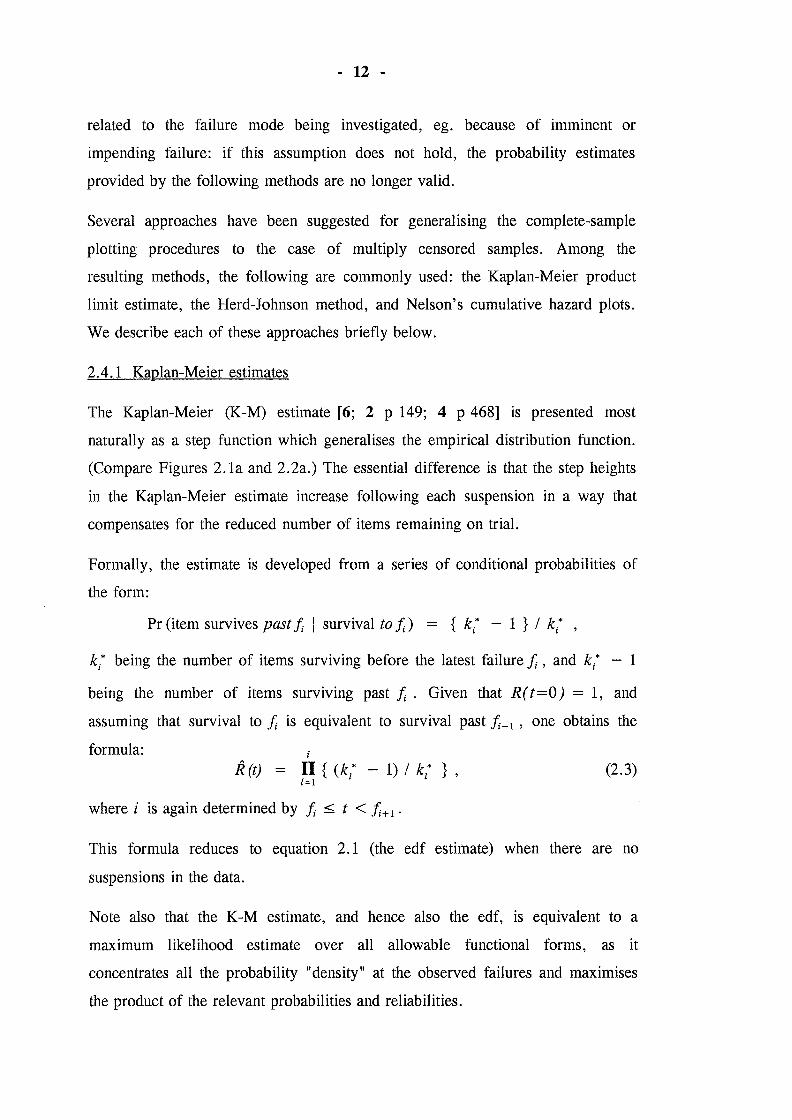
2.4.1 Kaplan-Meier estimates

The Kaplan-Meier (K-M) estimate [6; 2 p 149; 4 p 468] is presented most

naturally as a step function which generalises the empirical distribution function.

(Compare Figures 2.1a and 2.2a.) The essential difference is that the step heights

in the Kaplan-Meier estimate increase following each suspension in a way that

compensates for the reduced number of items remaining on trial.

Formally, the estimate is developed from a series of conditional probabilities of

the form:

Pr (item survives past h I survival to h) = { kt - 1 } I kt ,

kt being the number of items surviving before the latest failure h , and kt - 1

being the number of items surviving past h . Given that R ( t = 0) = 1, and

assuming that survival to h is equivalent to survival past h-t , one obtains the

formula: i

R (t) = U { (kt - 1) I kt } , l=l

(2.3)

where i is again determined by h ~ t < h+t.

This formula reduces to equation 2.1 (the edf estimate) when there are no

suspensions in the data.

Note also that the K-M estimate, and hence also the edf, is equivalent to a

maximum likelihood estimate over all allowable functional forms, as it

concentrates all the probability "density" at the observed failures and maximises

the product of the relevant probabilities and reliabilities.

- 13 -

2.4.2 Herd and Johnson methods

Herd's and Johnson's methods provide point estimates of reliability (see Figure

2.2b). Although these methods are usually treated as identical, they actually arose

from somewhat different motivations and assumptions, and were not identical as

originally presented.

Figure 2.2 - Reliability Plots for Multiply Censored Samples

Herd proposed his method [7 p 203] specifically for the situation where all

suspensions occur at failure events, and provided a formula for estimated

(s-expected) reliability at each failure event in such situations. Within this

restriction, he considers the number of items remaining in service beyond failure

f._ 1 and its associated suspensions (in our notation, this number is kt ), and notes

- 14 -

that the s-expected proportion of survivors to t from those remaining in service

beyondt_1 is k;* I (kt + 1); hence he derives the formula:

R; = R;_ 1 • kt I (kt + 1)

(with R0 = 1), or equivalently: i

n { k( 1 (k( + 1) }. [=1

(2.4a)

(2.4b)

In the case of a complete sample, these estimates coincide with the mean rank

estimates of equation 2.2b.

Instead of considering reliability estimates directly, Johnson [8, 9] proceeds by

modifying the order numbers of the failures to allow for the presence of earlier

suspensions. He does this by supposing that the suspended items remained in

service until they actually failed, and considering the possible orderings of events

that could result, depending on when these failures occurred. For each actual

failure, he then averages the order numbers that would result from each of these

scenarios8•

In terms of the notation introduced earlier, Johnson's formula for the modified

order numbers is: (2.5)

( with 111o = 0 ). The resulting modified order numbers9 m; are then used instead

of the original order numbers i in calculating the representative plotting positions

(section 2.3.2, equation 2.2). In the complete case, m; = i for all failures, and

the reliability estimates reduce to whichever of equations 2.2(a-c) is preferred by

the analyst.

The correspondence between Johnson's method and Herd's method arises if one

uses mean rank positions (equation 2.2b) to convert the modified order numbers

to reliability estimates10: identical estimates then result from both methods. This

8. A more detailed discussion of Johnson's derivation is presented in Chapter 5.

9. Johnson actually calls them mean order numbers, due to his method of obtaining them.

10. Johnson himself espouses median rank estimates (equation 2c), a proposal described by Nelson [2 p 148] as "a small and laborious refinement".

- 15 -

can be demonstrated by rewriting the LHS of equation 2.5 as mi:l- mi* and

solving for mi* : we get

mi· = mi:1 • ki* I (ki* + 1) (2.6)

(with m0* = n + 1), which clearly parallels Herd's result in equation 2.4a. This

correspondence shows that Johnson's results are equivalent to assuming that all

suspensions are actually concurrent with their respective preceding failures, and

then applying Herd's method to the adjusted data11; it also confirms that Herd's

reliability estimates are essentially an extension of the mean rank estimates for

complete samples.

Just as the point reliability estimates of section 2.3.2 lie within the steps of the

edf plot, it can also be shown that the Herd-Johnson estimates Ri always lie

within the corresponding steps of the Kaplan-Meier estimate. (Compare Figures

2.2a and 2.2b.)

2.4.3 Cumulative hazard plots

Instead of estimating the reliability level at each failure event, Nelson developed

a method which estimates the value of the cumulative hazard function H(t) at

these ages [10; cf. 2 pp 132.ff]. The resulting point estimates (H'''i ) are then

plotted against age in the usual way, but using paper whose scales are adapted to

cumulative hazard values instead of reliability values (see Figure 2.2c). An

equivalent formulation can also be derived for the reliability estimates R i by

using the relationships presented on page viii of the Notation section: see also 4

p 469; 10.

To obtain his estimate for H(t) at a given failure event h, Nelson adds together

individual estimates of MI(t) for each of the earlier intervals between failures.

11. Although Johnson does not explicitly assume that all suspensions are concurrent with failures, an assumption such as Herd's is required to justify Johnson's method of calculating the modified order numbers. (See Chapter 5 for details.) Thus, apart from the question of plotting positions, the two methods are essentially equivalent .

- 16 -

Denoting HAi - HAi-l as t::Jri, Nelson's estimates are given by

(2.7a)

yielding (since H(t=O) = 0): i

HAi = L { 1 I kl* } . (2.7b) 1=1

Each estimate Mri depends only on the number of items in service at the end of

the respective interval, ie. immediately prior to the corresponding failure :h - .as

though the hazard rate z(t=:h) applied throughout the entire interval. It follows ·

therefore that this formulation - like Johnson's - is insensitive to the timing of

the suspensions within the given intervals.

2.4.4 Effects of sample size

For censored samples with many failures, the methods discussed in this section

are hardly distinguishable from one another - nor from the methods of later

chapters. However, in samples with a small number of failures, the differences

between methods are quite noticeable. In particular, we shall see that the methods

presented later are noticeably more accurate than the methods above in cases

where there are many censorings and few failures.

2.5 Limitations of Existing Graphical Methods

The previous section describes several variants of the graphical method which are

widely used for the analysis of multiply censored samples. All of these methods

depend only on the number of items (kt) in service at each failure :h; as a result,

they are insensitive to the exact ages of the suspension events si , reflecting only

the order in which suspensions and failures occurred. Conversely, all of the

methods exhibit discontinuities in their reliability estimates if a suspension age is

varied - even marginally - so as to pass the age of a failure.

The methods we present in succeeding chapters contrast with these by being fully

and continuously sensitive to changes in suspension timing12•

12. An alternative way of describing this situation is to note that all the above methods require the convention mentioned previously (viz, that a failure notionally predates any concurrent suspensions) in order to guarantee consistent

- 17 -

The discontinuous sensitivity of the existing methods to suspension ages 1s

demonstrated by the following simple example.

Table 2.1 - Example Reliability Data (age in hours at failure I suspension)

Event Case 1 Case 2 Case 3 Case 4

fl 100 100 100 100

sl 102 150 198 -

h 200 200 200 200 (sl) - - - 202

MTBF 201 225 249 251

The data of Table 2.1 represent four possible results of a reliability trial

consisting of three items. Intuitively, one would expect cases 3 and 4 to be nearly

identical, and both to differ noticeably from cases 1 and 2, but this is not

reflected in the estimates provided by any of the methods discussed above. (See

Table 2.2 and Figure 2.313.) Instead, the reliability estimates R2 are constant

across cases 1 to 3 (and for any cases falling between them), but change

discontinuously from case 3 to case 4 (ie, as the age of suspension s1 passes that

of failure h).

Table 2.2 - Reliability Estimates from Example Data

Kaplan-Meier Herd-Johnson Cum. Hazard Case: 1 - 3 4 1 - 3 4 1 - 3 4

R1 0.666 0.666 0.75 0.75 0.717 0.717

Rz 0 0.333 0.375 0.5 0.264 0.435

We shall demonstrate in subsequent chapters that this inconsistency does not

apply to the improved estimation methods we shall present there.

results in such circumstances. This is not true of the improved methods we describe in later chapters.

13. F( values from the cumulative hazard method have been converted to the

corresponding reliability estimates R i •

- 18 -

Figure 2.3 - Reliability Plots for Example Data

2. 6 Currency of Existing Methods

Despite the long currency of the existing methods, the common limitation

described in section 2.5 does not appear to have been addressed previously. For

example, a citation search for Herd and Johnson (references 7 to 9) over the

years 1980 - 1996 found 71 citations, none of which dealt with improvements to

those methods. Consequently, it seems reasonable to claim that there are no

recent antecedents for the research reported in the following chapters.

2.7 Summary

In this chapter, we have described the basic aims of reliability analysis, the two

main approaches to estimating a reliability function from sample data, and the

basic elements of the graphical approach. We have considered the most common

graphical methods for analysing complete samples, and also their commonly used

generalisations to the case of multiply censored data.

We have demonstrated (from their definitions, and also by a simple example) that

these commonly used methods for analysing censored data are not continuously

sensitive to changes in the ages of the suspensions in the data set, and that this

insensitivity contradicts one's intuitive expectations for such estimates. Despite

their popularity, there is room for improvement in these methods.

Chapter 3: A Continuous Generalisation of the Herd-Johnson Formula

3. 0 Introduction

Among the methods discussed in the previous chapter for analysing censored

samples, the Herd-Johnson method is the most widely used, being cited in current

papers as a methodological reference1, and being the method presented by many

texts on reliability engineering [eg. 1 p 69, 11 p 316]. The reliability estimates

that it provides are not, however, continuously sensitive to changes in suspension

ages. In this chapter we present an estimation method which is continuously

sensitive to such changes, and which reduces to the Herd-Johnson formula in

appropriate circumstances.

By extending Herd's approach, we derive an improved formula for the estimated

reliability levels (Ri) at each failure; we also derive a reduced form for cases

with multiple simultaneous suspensions. We consider, both by argument and by

example, some desirable properties of the improved estimates. Finally, we

present the equivalent formula for calculating modified order numbers (~) from

the data.

3.1 Motivation for Generalisation

We recall firstly that Herd's derivation ([7 p 203]; section 2.4.2) applies only to

the restricted case where all suspensions occur at failure events. Within this

scenario, kt is the number of items remaining in service beyond failure i-1 and

its associated suspensions, and the s-expected proportion of survivors to i from

those remaining in service beyond h-l is kt I (ki* + 1); from this, one derives

the reliability estimates (cf equation 2.4a):

(R0 = 1). (3.1)

(Note that these estimates apply strictly at the ages h of the failures.) To

generalise this approach, we first consider Figure 3.1, which provides a

graphical expression of Herd's result for two different cases - one without

1. Reference 9 IS listed 16 times in the Science Citation Index for the period 1992-1996.

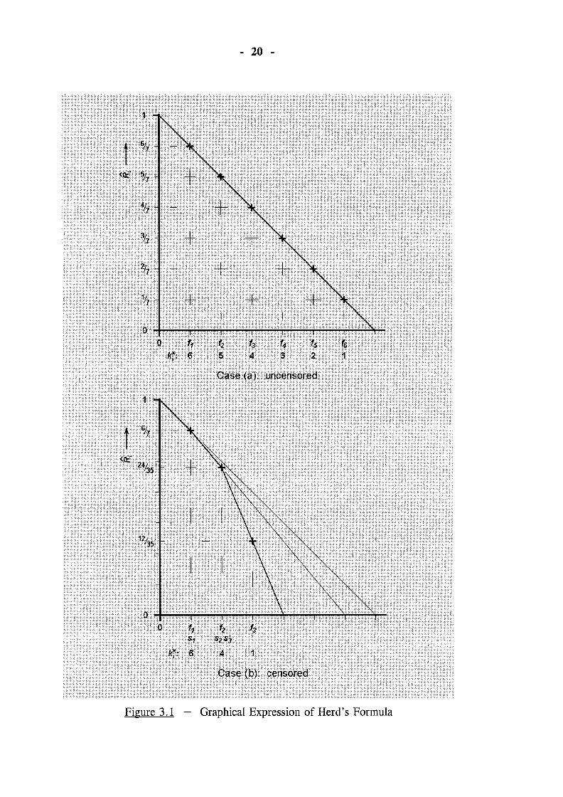
20

Figure 3.1 Graphical Expression of Herd's Formula

- 21 -

suspensions and one with suspensions as noted. Note in particular that this figure

plots estimated reliability against order number and not against age.

In both cases, testing commences with n = 6 items, and so (by equation 3.1) the

first failure occurs at an s-expected reliability of 6 17; this is represented on each

diagram by finding the ordinate corresponding to the intersection of the sloping

line and the first failure (i = 1). In the case with no suspensions (Figure 3.1a),

each succeeding failure}; corresponds to an s-expected fraction kt l(ki* + 1) of

the reliability for the previous failure, ie. to an s-expected reliability of

kt /(n + 1). The linearity (in ki*) of this latter expression is represented in Figure

3.1a by the uniform slope of the line from which the respective intercepts are

determined.

Turning to Figure 3.1b, the effect of the first suspension is to reduce by one the

number of items remaining in service from that time, and hence to increase the

s-expected number of failures (out of the original group of six) corresponding to

each further failure event. This is represented in our diagram by a corresponding

steepening of the reference line. Similarly, the two suspensions at the next failure

further reduce the number of items in service and correspondingly increase the

slope of the reference line - in this case by a factor of k; l(k3* + 1) = 4 /(1 + 1)

= 2.

The explanation above corresponds geometri~ally to the algebraic expressions

derived by Herd for the case where suspensions occur only at failure events. Now

consider a data set such as that of Figure 3.2, where the suspensions do not occur

exactly at failure events. According to the Herd-Johnson method, the reliability

estimate R 2 would be determined from the intercept of the broken line at age A

(point "b" on the diagram), but this approach fails to take account of the extra

service recorded by items s1 and s2 between the age ft and the ages of their

removals. The full line on the diagram (resulting in estimate "a") indicates a

more satisfactory alternative; we will formalise this alternative in the remainder

of this chapter.

- 22 -

Figure 3.2 - Graphical Representation for Suspensions Mid-Interval

In essence, we treat these cases by allowing the sloping line indicating the

reliability to continue with its gradient unchanged until it reaches the age at which

a suspension occurs. The gradient increases only at the actual age of suspension,

instead of at the preceding failure, a change which reflects that item's suspension

age more accurately in the ensuing calculations.

3.2 Derivation of Improved Reliability Estimates

3.2.1 The improved estimates

For each suspension sj, define the fraction cxj = (sj -h-1 ) I (h -h-1 ) (where2

h-1 < sj <h); also, let k; = n + 1, R0 = 1, and suppose (for convenience)

that the suspensions between h-1 and h are sm , . . . , sM. Then the improved

reliability estimates corresponding to equation 3.1 (cf equation 2.4a) are:

2. In principle, h-1 :;e. h for all values of i; section 3.5 discusses possible concerns and remedies when the data do not satisfy this condition.

k.* l

or equivalently (cf equation 2.4b):

k.* l

n+1

- 23 -

n (k/ +1-a)

j=m (k/ -aj)

It (k/ +1-a)

j=1 (k/ -a)

(3.2a)

(3.2b)

As these estimates arise from an extension of Herd's approach (section 2.4.2),

these also are essentially mean rank estimates.

3.2.2 Derivation of estimates

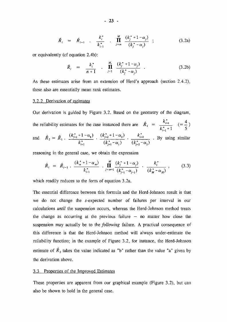
Our derivation is guided by Figure 3.2. Based on the geometry of the diagram,

the reliability estimates for the case instanced there are R 1

and Rz = R1 . (kj:1 + 1-a1) (kj:2 + 1-az) ki:z

ki:1 (kj:1 -a1) (kj:2 -az)

reasoning in the general case, we obtain the expression

n (k/ + 1-aj) j=m+1 (k.* -a. )

;-1 ;-1

which readily reduces to the form of equation 3.2a.

ki:1 4 = (=-)

ki:1 + 1 5

By using similar

k.* l (3.3)

The essential difference between this formula and the Herd-Johnson result is that

we do not change the s-expected number of failures per interval in our

calculations until the suspension occurs, whereas the Herd-Johnson method treats

the change as occurring at the previous failure - no matter how close the

suspension may actually be to the following failure. A practical consequence of

this difference is that the Herd-Johnson method will always under-estimate the

reliability function; in the example of Figure 3.2, for instance, the Herd-Johnson

estimate of R2 takes the value indicated as "b" rather than the value "a" given by

the derivation above.

3. 3 Properties of the Improved Estimates

These properties are apparent from our graphical example (Figure 3.2), but can

also be shown to hold in the general case.

- 24 -

Proposition: The reliability estimates presented in equation 3.2 have the

following properties:

a. they reduce to the Herd-Johnson estimates in the special case

where all suspensions occur at failure events;

b. they are sensitive to changes in suspension ages, with increased

service life for a suspended item resulting in increased reliability

estimates for subsequent failures;

c. they do not jump discontinuously when suspension ages change

from just before to just after a nearby failure event.

Proof: To verify statement (a), consider the typical interval [.{;_ 1 ,.t; ), and put

aj = 0 for j = m ... M; since ki:I = k; + 1, kj:I = k/ + 1 within this interval,

and k; = kt + 1, each of the ratios in equation 3.3 is unity except for the final

one, which has the value ki* l(ki* + 1), as required.

Next, consider equation 3.2. Provided that sj <J;, an increase in any aj

increases the corresponding factor in the product, and hence increases R i ; this

verifies statement (b).

Finally, suppose that sM is the q-th event (ie, Eq) and that.{; is Eq+I, and

let aM~ 1 (ie, sM ~ .t; ); the final ratio in equation 3.2a then approaches

q* l(q* -1), while the term kt is equal to (q + 1)* = q* -1. Alternatively, if

sM = .t; then sM becomes Eq+I and .t; becomes Eq, so that the term containing aM

disappears from the product and the term k/ becomes q*, while all other terms

remain unchanged. From these remarks it follows that the estimate Ri is

continuous as sM passes .t;. A similar argument using the equation for Ri+I shows

that reliability estimates at all later failures are also continuous as sM passes .t;,

and so we have demonstrated that statement (c) is also satisfied. [QED]

- 25 -

3.4 Simplified Form for Grouped Suspensions

When multiple suspensions occur simultaneously the general formula given above

still applies, but it may be more convenient (particularly when performing

calculations by hand) to take advantage of the following simplified formula.

Instead of using the index j to order the suspensions individually (s1 ... si ... ),

we use a new index J to order the groups of suspensions (s1 • • • s 1 • • • ) ; we note

also the number of suspensions N1 in each group. The event index k1 must still

incorporate the full number of earlier suspensions (not just the number of groups

of suspensions); under this proviso, k1 is defined naturally as the event index

corresponding to the first time the J-th group is encountered.

Proposition: Using the above notation for grouped suspensions, the reliability

estimates Ri of equation 3.2 may also be calculated as

k.* I

n+1

M,

n J=l (k * + 1 - N -ex )

J J J

(3.4)

where cx1 denotes the common value of cxi for the suspensions in the J-th group.

Proof: In the previous notation, the group of simultaneous suspensions will of

course be numbered consecutively: suppose that the values of j corresponding to

group J are l ... L ; these suspensions will also have identical values of cxi . As in

the proof of section 3, we have ki:1 = k/ + 1 within this group, and several of

the ratios in the product of equation 3.3 will therefore reduce to unity; the

remaining ratios will mention only the first and last suspensions of the group (in

the numerator and denominator respectively). The implication for equation 3.2 is

that the terms in its product corresponding to the group of suspensions may be

replaced by the single ratio (kt + 1-cx1 )l(k{ -cx1 ) . Since k1* = k; and

k{ = k1* + 1-N1 , equation 3.4 follows. [QED]

3.5 Treating "Simultaneous" Failures

The case of multiple simultaneous failures requires special mention. Two

situations should be distinguished, namely those where the failures are (s-)

- 26 -

independent of one another and those in which the failures are due to a common

cause. In the former case, the probability of two items failing at precisely

identical ages is theoretically infinitesimal, but the coarseness of the age

measurements may result in identical recorded ages: we discuss this case below.

In the second case none of the estimation methods discussed in this thesis applies

(including the existing methods discussed in chapter 2), as all such methods rely

on the basic assumption that the performance of each item in the sample is s­

independent from that of all the others: in practice, the factor causing the

multiple failures should be investigated - and may itself be suitable for the

methods of analysis discussed here!

If several independent failures are recorded as having the same age, a certain

amount of judgement may be necessary in completing the analysis. Firstly we

note that the two or more failures must be considered separately, even though the

resulting reliability estimates will all be plotted against the same age; thus, each

will have its own k* value and will be given its own R value.

If there are no suspensions simultaneous with the failures, then the equations

above (equation 3.2 or equation 3.4) may be applied in a straightforward manner,

and no further comment is necessary. We are left therefore with the case of one

or more suspensions simultaneous with "multiple" failures.

If the measurement inaccuracy is small, it is reasonable to assume (or it may be

known anyway) that the suspensions have actually lasted as long as all the

recorded failures did; in this case, the usual convention may be employed, ie. the

failures are treated as occurring first and the suspension(s) as occurrmg

immediately afterwards. If, on the other hand, the measurement inaccuracy is

large, some guess must be made as to the relative timing of the suspensions and

failures. The most conservative assumption (ie, the one resulting in the lowest

estimates of reliability) is that the suspensions occurred first, the most

"unconservative" assumption is the usual convention (that the failures occurred

first), and a reasonable compromise is to associate the suspensions with the

middle failure. (Take the "next" failure after the middle if there is an even

number of failures in the group.)

- 27 -

3. 6 Examples

We use the following examples to compare our improved reliability estimates

with those obtained from the Herd-Johnson method. In particular, we contrast the

continuous sensitivity of the improved estimates against the insensitivity I

discontinuity of the Herd-Johnson estimates3•

3.6.1 Numerical example

Table 3.1 contains data (Case 0) originally presented by Johnson [8 p70],

together with three variations (Cases 1-3) which illustrate the properties of the

improved estimates. The Herd-Johnson estimates and the improved estimates for

these four cases are presented in Table 3.2, and are also plotted in Figure 3.3;

the curves of Figure 3.3 have been fitted using Weibull probability plots.

Table 3.1 - Variations of Johnson's Example Data (age in hours at failure I suspension)

Events Case 1 Case 0 Case 2 Case 3

!t 112 112 112 112

sl 112 213 249 -

fz 250 250 250 250

(sl) - - - 250

Sz 250 484 571 -

s3 250 500 571 -

h 572 572 572 572 (Sz) - - - 572 (s3) - - - 572

Table 3.2 - Reliability Estimates by Case and Estimation Method

Case 1 ~ Case 0 Case 2 ~Case 3 . Estimate Both H-J Eq 2 H-J Eq 2 Both

R.l 0.857 0.857 0.857 0.857 0.857 0.857 . Rz 0.686 0.686 0.705 0.686 0.7140 0.7143

A

R3 0.343 0.343 0.461 0.343 0.534 0.536

3. The discussion of the previous chapter indicates that the reliability estimates obtained from the other existing methods behave in a similar fashion to those of the Herd-Johnson method, so we will not consider them separately.

- 28 -

Figure 3.3 - Reliability Plots of Example Data

The improved estimates can be seen to display the properties described in

section 3.3; in particular, the resulting curves indicate a smooth and gradual

transition between the various cases, while those fitted to the Herd-Johnson

estimates will clearly jump from the lower curve to the upper curve as the

suspensions pass the failure ages.

This example also demonstrates that the Herd-Johnson estimates are always

pessimistic - except for those (few) samples where the suspensions occur only at

the failure ages.

3.6.2 Theoretical example

As a further indication of the difference between the improved estimates and the

Herd-Johnson estimates, consider a data set comprising four items, and suppose

that one of these items is suspended at some stage. If we consider the effects on

our reliability estimates (R 1 , R2 and R3 ) of varying the suspension age, we

obtain the comparison in Figure 3.4: the reliability estimates are plotted as

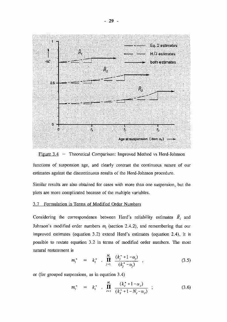
- 29 -

Figure 3.4 - Theoretical Comparison: Improved Method vs Herd-Johnson

functions of suspension age, and clearly contrast the continuous nature of our

estimates against the discontinuous results of the Herd-Johnson procedure.

Similar results are also obtained for cases with more than one suspension, but the

plots are more complicated because of the multiple variables.

3.7 Formulation in Terms of Modified Order Numbers

Considering the correspondence between Herd's reliability estimates Ri and

Johnson's modified order numbers mi (section 2.4.2), and remembering that our

improved estimates (equation 3.2) extend Herd's estimates (equation 2.4), it is

possible to restate equation 3.2 in terms of modified order numbers. The most

natural restatement is

m.* I

li (k/ + 1-o) kt . i=l (k/ -a)

or (for grouped suspensions, as in equation 3.4)

m.* I

k .* • [i ( k; + 1 - a) 1

J=t (k * + 1- N -a ) J J J

(3.5)

(3.6)

- 30 -

to obtain the values of mi directly, one instead subtracts the relevant expression

above from n + 1.

These values of mt (or mi) may be useful to those who prefer to base their

reliability estimates on median ranks (equation 2.2c) rather than mean ranks, as

they may be treated equivalently to the (reverse) order numbers i* (or i) for a

complete sample.

3.8 Summary

In this chapter we have considered the calculation of reliability estimates for

general multiply censored data. Recalling from chapter 2 that the Herd-Johnson

estimates are only justified for a restricted class of samples (viz, those in which

suspensions occur only at failure events), we have considered the justification for

that approach and have presented an extension of it which provides suitable

estimates for the un-restricted case.

The improved estimates we have presented, unlike those of existing methods, are

continuously sensitive to all changes in suspension ages; in particular, they do not

jump discontinuously when the age of a suspension is varied marginally so as to

pass the age of a nearby failure. The improved estimates also reduce to the Herd­

Johnson estimates in cases where the latter apply. We have proved these

properties formally, and have also demonstrated them through suitable examples.

In addition, we have presented and justified a simplified formula for calculating

the reliability estimates in cases where the data contains groups of simultaneous

suspensions, and have presented an equivalent formula for estimating modified

order numbers from the data.

Chapter 4: An Improved Variant of the "Hazard Plotting" Method

4.0 Introduction

The results of this chapter are similar to those of the previous chapter, except that

we take a different graphical method for our starting point, namely Nelson's

"hazard plotting" method (section 2.4.3).

The cumulative hazard estimation method ("hazard plotting" method) presented

by Nelson [10; 2 p 132ff] is another commonly used graphical method for

estimating sample reliability functions [1 p 82; 4 p 469]. This method shares the

limitations discussed in chapter 2 for all existing graphical methods, namely

insensitivity to changes of suspension ages within an interval between failures,

and discontinuity with regard to changes of suspension ages between adjacent

intervals. We present below an improved version of this method which - like the

reliability estimates derived in chapter 3 - is continuously sensitive to changes in

suspension ages; in this case, the improved method reduces to Nelson's method

in appropriate circumstances.

We first motivate our method using arguments appropriate to the hazard plotting

approach, and present the resultant formula for the cumulative hazard estimates

Hi. We then prove the desired continuity properties for these estimates, and

provide an illustrative example to compare the improved estimates with those

from Nelson's method.

4.1 Deriving the Improved Hazard Plotting Method

4.1.1 Motivation for changes

Our alternative to Nelson's approach is based on similar considerations to those

advanced in chapter 3 for generalising the Herd-Johnson method, viz. finding an

approach that does not assume a restricted set of suspension ages. We recall from

chapter 2 (section 2.4.3) that Nelson's approach is equivalent to assuming that all

suspensions actually occurred at the immediately preceding failure; in fact, we

note further that Nelson's justification of his method [10 p 963] is based on the

case where suspensions occur only at failure events. In particular, Nelson's

- 32 -

estimated cumulative hazard increment !lHi for the interval [.t;_1 ,:t;) reflects only

the hazard rate applying after the last suspension (if any) in this interval.

The inconsistencies of this approach can be seen by considering the data sets of

Figure 4.1. In the first two cases, there is a noticeable difference between the

typical numbers of items at risk in the various intervals, but Nelson's approach

gives identical results. On the other hand, the second and third cases have very

similar typical numbers at risk, but are given quite different estimates by

Nelson's method.

Figure 4.1 - Numbers at Risk vs Age for Various Samples

A more realistic approach, ie. one which better represents the variety of

suspension ages that may be observed, is to calculate !lHi as a weighted average

of the hazard rates applying after each of the observed suspensions; the obvious

weighting factor for such an estimate is the relative lengths of the sub-intervals

between suspensions.

4.1.2 Improved estimates for cumulative hazard values

Proceeding on this basis, we suppose again that the suspensions in the interval

[:f:_1 ,fD are sm ... sM, and define weighting factors {3m ... {3M and {3i as follows:

- 33 -

With this notation, the improved estimates for the hazard increments are

A (3 i M (3j b.H. = - + :E -

I k* ·- k* ' i ;-m j

(4.1a)

and hence the cumulative hazard estimates are

(4.1b)

4.1.3 Multiple suspensions and "multiple" failures

When multiple suspensions occur at the same age, the (3i value corresponding to

the second and subsequent suspensions will equal zero, reducing the number of

non-zero terms in equation 4.1. Although there is no resulting simplification in

the form of the equation, an awareness of this fact may save some computation

time when analysing a data set by hand: the general rule is that only the first

suspension in each group needs to be included in the summation.

The case of multiple failures at a given age was discussed in chapter 3 (section

3.5) in relation to the estimates developed in that chapter. The comments in that

section also apply to the estimates of this chapter, ie. common cause failure

should prompt an investigation of the causative factors, while "multiple" failures

due to coarseness of measurement may require some exercise of judgement if

there are suspensions simultaneous with the "multiple" failures. In such cases, the

guidelines of section 3.5 may be applied to the estimates of this chapter also; in

addition, however, the convention footnoted above regarding the assignment of

1. In principle (as in Chapter 3), h-1 ;r. h for all values of i; section 4.1.3 (see also section 3.5) discusses possible concerns and remedies when the data do not satisfy this condition. As a minimum, we must then provide alternative definitions for certain (3 values (see next footnote).

2. If h-1 = h, the (3 values defined here reduce to 0 I 0 ("undefined value") for any events in the "interval" (h_1 ,h]. In this case it is most reasonable to define (3i = 1 for the failure h and (3i =0 for any suspensions si associated with h-1 (see section 4.1.3 below). This ensures that every failure event has a direct effect on the hazard estimates, as with the current method.

- 34 -

values to the weighting factors (3i is essential in all cases of "multiple" failures

(ie, whether or not there are any simultaneous suspensions).

4.2 Properties of the Improved Estimates

As in the previous chapter, these properties follow readily from the arguments we

have used to motivate the derivation of the improved method. Properties (b) and

(c) are identical to those for the improved estimates of the previous chapter.

Proposition: The reliability estimates presented in equation 4.1 have the

following properties:

a. they reduce to Nelson's cumulative hazard estimates (equation

2.6) in the special case where all suspensions occur at failure

events;

b. they are sensitive to changes in suspension ages, with increased

service life for a suspended item resulting in decreased estimates of

cumulative hazard (ie, increased reliability estimates) for

subsequent failures;

c. they do not jump discontinuously when suspension ages change

from just before to just after a nearby failure event.

Proof: To verify statement (a), consider the typical interval [J;_1 , .t; ), and put

(3j = 0 for j = m ... M ; then (3i = 1 and the required results follows immediately.

Now consider a suspension sj , and suppose that Eq is the next event

(failure or suspension); any increase in the age sj also increases cxj: hence (3j will

increase and (3q will decrease by the same amount. Consider any failure .t; > sj;

since k/ > q*, the effect on equation 4.1 (of the increase in sj) will be a net

decrease in the cumulative hazard estimate. This verifies statement (b).

Finally, suppose that EP is the event immediately previous to sM, and

define ex; as {cx.M_1 if EP =sM_1; 0 if EP =J;_1 }. As sM....,_. .t;, the first term in

equation 4.1a approaches zero, while the final term in the summation approaches

(1- cx;)l(p + 1)* . When sM = .t;, the term containing cxM disappears from the

- 35 -

summation, while h becomes Ep+I and the first term thus becomes

(1- a;)l(p + 1)* . All the other terms in equation 4.1a remain unchanged, so it

follows that A.Hi, and hence Hi, is continuous as sM passes h. Since the equation

for fli+l is clearly continuous in sM for sM >h, this also proves statement (c) for

any later failures. [QED}

Figure 4.2 - Reliability Plot of Example Estimates

4.3 Worked Example

We consider again the data presented in the numerical example of chapter 2

(section 2.5, Table 2.1), and compare our improved cumulative hazard estimates

(equation 4.1) with those of the existing method (equation 2.6). The data is

presented again below as Table 4.1, and the resulting estimates of cumulative

hazard (HJ are presented in Table 4.2.

- 36 -

Table 4.1 - Example Reliability Data (age in hours at failure I suspension)

Event Case 1 Case 2 Case 3 Case 4

!t 100 100 100 100

St 102 150 198 -

fz 200 200 200 200 (st) - - - 202

MTBF 201 225 249 251

Table 4.2 - Comparative Estimates from Example Data

Cases 1-3 ~ Case 1 Estimate: Nelson

0.3333 0.3333

Case 2 Equation 4. 1

0.3333

Case 3

0.3333

Case 4 Nelson Eq 4.1

0.3333 0.3333

R1 0.7165 0.7165 0.7165 0.7165 0.7165 0.7165 .......................................................................................................................................................................................... 0 0 0 0 0 0

~:~:!: ! ~:~~:~ ~:~::~ ~:::~! ! ~:!!~: ~:!!~:

The corresponding reliability values (Ri) are also presented in Table 4.2, and are

plotted in Figure 4.2. It is apparent from this plot that the improved estimates

display the desired continuity as the age of s1 increases, while the existing

estimates do not.

4.4 Summary

In this chapter we have generalised the cumulative hazard estimates presented by

Nelson to the case of general multiply censored data. As with the Herd-Johnson

estimates considered in chapter 3, the existing cumulative hazard estimates are

only justified for a restricted class of samples, viz. those in which suspensions

occur only at failure events. We have again presented a simple extension of the

original argument which provides suitable estimates for the un-restricted case.

The improved estimates of this chapter - like those of the previous chapter

are continuously sensitive to all changes in suspension ages and, in particular, do

not jump discontinuously when the age of a suspension is varied marginally so as

to pass the age of a nearby failure. As would be expected, the improved estimates

- 37 -

of this chapter reduce to the existing cumulative hazard estimates in cases where

the latter are justified. We have proved these properties formally, and have

demonstrated them by a simple example.

Issues and simplifications which may arise in cases with simultaneous suspensions

and I or simultaneous failures have also been discussed.

Chapter 5: Better Estimates for Modified Order Numbers

5. 0 Introduction

In this chapter, we examine Johnson's concept of modified order numbers and

develop an alternative expression for calculating these quantities. We show again

that Johnson's estimates are only justified in cases where all suspensions occur at

failure events, and we present two alternatives to Johnson's method of estimating

the quantities involved.

The first of these alternatives is equivalent to the method presented in chapter 3.

We have already shown that this method provides reliability estimates that are

continuously sensitive to changes in suspension ages, whereas Johnson's method

does not.

The second alternative requires the existence of an initial estimate for the

reliability function R(t), and provides a method for further refining such an

estimate; we therefore denote this alternative as the "Second Stage" method. We

present the details of this method below, and demonstrate that it also provides

reliability estimates that are continuously sensitive to changes in suspension ages.

5.1 Modified Order Numbers and "Notional Failures"

5 .1.1 General discussion

As we noted in chapter 2, Johnson's approach to analysing multiply censored data

is to modify the order numbers of the failures to allow for the presence of any

earlier suspensions; the plotting positions R i are then calculated by usmg the

modified order numbers mi instead of the original order numbers i in the

formulae of section 2.3.2. We examine this approach in some detail, in order to

separate the basic justification for modified order numbers from Johnson's

particular estimates of these quantities.

Following Johnson's derivation [8 ch 8], we consider what might happen to the

items which were suspended in our actual sample if these items had all been

allowed to remain in service until failure; in particular, we are interested in how

the order numbers of the actual failures would be affected under each possible

- 39 -

outcome of our conceptual trial. Our aim is to obtain a set of modified order

numbers mi , each of which estimates the average order number (out of n ) that

the corresponding failure h would have if all items had failed.

In considering the possible outcomes of our trial, we note that the order number

of failure h would only be affected if an earlier suspensions sj were to fail

between the ages sj and h , in which case the order number would increase by 1

for each suspension satisfying this condition, ie. for each "notional" failure

occurring before h . The order number adjustment Ai = mi - i therefore

depends on the possible failure ages of the suspensions prior to h .

If we focus on an individual suspension sj , we see that its average contribution to

Ai (over all possible outcomes) is just the probability of its failing between the

ages sj and h - assuming that it had remained in service beyond sj • Denoting this

probability as pij, we obtain the following expressions:

M,

Ai - .L Pij (5.1a) j=l

M,

mi - i + .L Pij (5.1b) j=l

and also M,

m.* - k.* + .L rij (5.1c) I I

j=l

In equation 5 .1c, rij = 1 - pij is the probability of suspension sj surviving

beyond age h, while the equivalence of equations 5.1b and 5.1c is established via

the relationship i + Mi = ki . This equation is more convenient to use than

equation 5 .1b, because the desired reliability estimates Ri relate directly to the

reverse order numbers mi* given by this equation (see equation 2.2). As

demonstrated further below, the quantities rij are also easier to calculate than the

corresponding values of pij.

5 .1. 2 Johnson's assumption

We noted in chapter 2 that Johnson's estimates for the modified order numbers

result from a particular way of averaging the possible order numbers of the actual

failures: in terms of equation 5.1 above, this corresponds to one particular way of

- 40 -

estimating the probabilities pij. We demonstrate in this section and the next that

Johnson's method of averaging is only justified in the restricted case where

Herd's condition applies, ie. when all suspensions are concurrent with failures. In

later sections, we present an improved alternative for the general case where

Herd's condition does not apply.

We noted above that the order number of a failure/;_ in our conceptual trial would

only be affected by suspensions sj which fail before the age/;_ . For any particular

outcome, this means that the order numbers of the actual failures depend on the

order in which the actual and notional failures occur. Johnson uses this fact as a

basis for calculating his modified order number estimates: he proceeds by

averaging over the number of possible orderings of events that could result from

the trial, ie. by assuming that each of the possible orderings is equally likely.

When Herd's condition applies, this is a reasonable assumption - in fact, it is

equivalent to Herd's argument for his own reliability estimates - but we can

easily show that it is not reasonable in other cases.

Consider a sample in which one of the suspensions occurs shortly before a given

failure, but some time after the previous failure: clearly, the chance of this

suspension failing before the following failure is quite small, and so the

corresponding orderings should receive little weight when averaged with those

resulting from a later failure of that suspension. However, Johnson's method

gives these unlikely orderings the same weighting as it gives the other "later"

orderings. Thus we see that Johnson's implicit assumption of equal weightings is

not correct in the general case. We formalise this argument more fully in the

following section.

5.2 Johnson's Estimate for the Notional Failures

In the previous section we demonstrated that estimation of modified order

numbers mi is equivalent to estimation of the probabilities pij (or r ij) of each

suspension sj failing before (surviving beyond) the age /;_ if it had remained in

service until it failed. In this section, we derive the specific estimates of pij and

rij corresponding to Johnson's method.

- 41 -

Figure 5.1 Graphical Representation of Johnson's Modified Order Numbers

- 42 -

5.2.1 Deriving the estimates

In order to derive these estimates, we make explicit use of the correspondence

between Herd's and Johnson's method that we demonstrated in chapter 2, namely

Ri = mt I (n+ 1) . (5.2)

(See section 2.4.2.) We also use a graphical argument similar to the one we used

to describe Herd's method in chapter 3. (See section 3 .1.)

Consider first a specific example: suppose that six items are placed on trial, of

which one is suspended between the first and second failures and another between

the third and fourth failures. The modified order number estimates (mi or mt)

for this example are illustrated by Figure 5.1: part (a) shows the relationship

between mi and i, and part (b) shows the complementary relationship between

mi* and ki* . (Part (b) is equivalent to our treatment of Herd's reliability

estimates in section 3 .1, but with m t as the ordinate instead of R i • )

It is useful to compare the order number estimates of part (a) (represented by the

upper sloping line on the diagram) against the reference line mi = i , which is

the lower line on the diagram. The difference between these lines at each age/;.

represents the adjustment Ai = I: pij used to obtain the modified order number mi

from the original order number i . In a similar way, the difference in part (b)

between the reverse modified order numbers mi· and the discontinuous reference

line mt = kt is the summation I: rij of equation 5 .1c. These correspondences

are identified specifically in Figure 5.2, which combines the two parts of Figure

5.1 into a single diagram.

Figure 5.3 presents a further graphical example, in order to illustrate the

extension of these principles to larger samples and to those with more than one

simultaneous suspension.

By considering the above examples it is possible to develop expressions for the

probability estimates pij and rij corresponding to Johnson's method. Defining I

- 43 -

Figure 5. 2 - Combined Representation of Figure 5.1

(strictly, ~) as the next failure after si , the estimates rii are clearly given by

i

rij = n { (kt -1)/ kt } . 1=1

(5.3)

The corresponding estimates for pii are most easily obtained from these by using

the relationship pii = 1 - rii.

The correspondence between equation 5. 3 and Herd's reliability estimates

(equation 2.4) is obvious, and follows directly from Herd's arguments about the

s-expected proportion of suspensions that would have failed by the age of the

following failure. Equation 5.3 can also be described in words by remarking that

the "unassigned" suspensions remaining at any step are distributed equally over

the remaining intervals foreseen at that stage.

A procedure can be stated for obtaining the estimates pii "directly" (ie, without

calculating rii ), but its description is slightly clumsy - precisely because pii is not

- 44 -

Figure 5.3 - Graphical Representations: Further Example

the primary quantity being estimated. The procedure can be broadly summarised

as:

divide the item sj (one notional failure) equally between the k1* + 1

intervals [.fr_ 1 , fr ),

unless I until another group of suspensions is encountered beyond fr ,

in which case the number of remaining intervals is reduced (the

suspensions in the newly encountered group are removed from

consideration in counting the future intervals) and the increment in

pij for failures C beyond the new suspensions is adjusted

accordingly.

- 45 -

Thus p1J = ll(k1* + 1), Pr+lJ = 2/(k1* + 1), and so on, until the next group of

suspensions is encountered.

In this qualified sense, Johnson's method assumes equal likelihood of a

suspension failing in any subsequent interval between failures.

5 .2.2 Evaluating the estimates

We have noted previously that variations of the age sj within the interval

[fr_1 , fr) have no effect on Johnson's estimates for mi, and hence for Ri, even

though these variations may indicate a noticeable increase or decrease in the

satisfactory service life of the item being investigated. From the above analysis, it

is clear that the same is true of the pij and rij estimates corresponding to Johnson's

method.

We did not assume in our examples above that Herd's condition applies, ie. that

each suspension is concurrent with a failure. However, when this condition does

apply, the diagrams presented correspond exactly to Herd's method of estimating

reliability values (cf section 3.1). In this case, the resulting estimates for fnt and

mi* are perfectly justified: in particular, the probabilities of a suspension failing

in any of the subsequent intervals between failures are equal (in the sense

described above), and the adjustment Ai is equal in each case to the s-expected

number of notional failures in the interval [0, .t; ).

These statements are clearly not true in the general case - ie, when Herd's

condition does not apply; for example, the probability of a suspension sj failing

before the next failure fr becomes negligible when the two events are "very close"

(ie, when aj-1). Equally, the adjustment Ai corresponding to Johnson's method

is not equal to the s-expected number of notional failures in the interval [0, .t;)

unless the suspensions concerned each occurred at one or other of the recorded

failures. We conclude that Johnson's method, by averaging over the number of

possible orderings without considering their relative likelihoods of occurring,

produces biased estimates of the mean (s-expected) order numbers arising from

the conceptual trial.

- 46 -

5. 3 An Improved Estimation Method

We have noted repeatedly that Herd's condition is frequently not met in practice:

samples often occur in which suspensions happened at times other than failure

events. By the same argument that we presented in chapter 3, the estimation

process for the probabilities rij (or pij) should reflect the ages at which these

suspensions actually happened.

Figure 5.4 - Graphical Representation for Suspensions Mid-Interval

One way of doing this is to apply the arguments of chapter 3 to our estimation of

the suspension reliabilities rij. Consider Figure 5.4 (previously presented as

Figure 3.2): by changing the slope of the reference line only when a suspension

is encountered, rather than at the previous failure, we obtain estimates for each of

the ry's which do reflect the actual ages at which the suspensions occurred.

The resulting estimates for r ij are

nM, (k.* + 1-a.) r .. = J J

lJ . (k * ) J=I . -a. J J

(5.4)

- 47 -

Noting from any of the diagrams above that rif and /( diminish in the same

proportion at any given age :h, it follows that this method of estimating rif (or pif)

is entirely equivalent to the method for estimating R i presented in chapter 3.

5.4 An Alternative Improvement - the Second Stage Method

The method described in section 5.3 does not assume any particular distribution

form, so it is essentially a non-parametric method for estimating the quantities rif,

and hence Ri. In some cases, however, one may be interested in fitting a

particular distributional form, in which case the following alternative can provide

a suitable method for refining any "first estimate" RP (t) for the reliability

function R(t) 1•

5 .4.1 Derivation and formula

Suppose that we have an initial, usually parametric, estimate RP (t) for the

reliability function R(t) applying to the items of interest. By using the survival

information incorporated in this estimate, we can estimate the adjustments "E.pif or

"E.rif more accurately, and hence obtain improved estimates for the modified order

numbers mi or mi* . These can then be converted to reliability estimates R i in the

usual way, resulting in an improved estimate - the "second stage" estimate -

for the reliability function R(t).

In deriving the appropriate adjustments, it is easiest to work in terms of the

probabilities r if . Note again that rif is the probability that the item si survives until

age :h given that it has already survived until age si ; in other words it is a

conditional probability of survival. Using the symbol R(:h I si) to represent this

conditional reliability, we have

(5.5a)

1. Although the methods of this chapter are most naturally associated with the reliability estimation method of Chapter 3, any reasonable method may be used to provide an initial estimate: this includes the methods presented in Chapters 3 and 4 and also (but less desirably) the existing methods discussed in Chapter 2.

- 48 -

We can now use the initial estimate RP (t) to estimate R(E) for the relevant

failures and suspensions, and hence to obtain our rij estimates. Introducing the

simplified notations R{ and RJ as shown, we have

(5.5b)

and these values can now be substituted into equation 5.1 to obtain the modified

order numbers mt. The procedures normally used for complete samples may

then be followed.

5.4.2 A simplified formula for computations

For computational purposes, it is easier to combine equations 5.1 and 5.5 into a

single formula, namely

m.* I

k.* I +

M,

R{ L (1 I R~) . j=l J

(5.6)

By keeping a running total of the summation (updated each time a new

suspension becomes relevant), each of the R{ and RJ terms need only be

calculated once. This procedure is demonstrated in the numerical examples of

section 5. 5 .1.

The order number estimates m t from equation 5. 6, like those from equation 5.1 ,

may still be transformed to whichever type of reliability estimate (mean rank,

median rank, etc.) the analyst may prefer.

5.4.3 Properties of the improved estimates

The second stage method proposed above retains the properties (b) and (c) that

applied to our previous proposals (chapters 3 and 4), namely, completely

continuous sensitivity to changes in suspension ages. In particular, an increased

age at suspension si (<h) results in a higher conditional probability rij , a larger

estimate for mi* (ie, a smaller estimate of mi ), and hence a higher estimated

reliability level at h . More formally, we have:

Provosition: Provided that the initial reliability estimate RP (t) varies

- 49 -

continuously with item age t , then the modified order number estimates derived

from equations 5.1 and 5.5 have the following properties:

a. they are sensitive to changes in suspension ages, with increased

service life for a suspended item resulting in increased estimates ofmt

(and hence, in increased reliability estimates Ri) for subsequent

failuresh;

b. they do not jump discontinuously when suspension ages change

from just before to just after a nearby failure event.

Proof: Statement (b) follows directly from the continuity of the initial estimate

RP (t) : in particular, the fact that RP ( sj) varies continuously without regard to the

ages at which failures occurred in the sample.

To verify statement (a), note that any increase in the value of sj must

decrease RP ( sj), thereby increasing rif for any later failures h, and so increasing

m.* for these failures. I

[QED]

Comments: The requirement for continuity of RP (t) in not restrictive in practice,

since all parametric estimates (and most non-parametric estimates) are continuous:

in fact, this is an intuitive requirement for a properly "representative" reliability

function estimate for real-world items.

We note also that any stationary behaviour accepted in RP (t) - usually restricted

in practice to an initial "failure-free" period - will be reflected in similar

behaviour of rif and mi* whenever sj lies within the relevant interval of ages. This

assumption about RP (t) will therefore be reflected also in the estimates Ri

generated from them.

5.5 Numerical Examples

The method presented in this chapter was originally developed in the context of

fitting a Weibull distribution, and the examples presented here use this

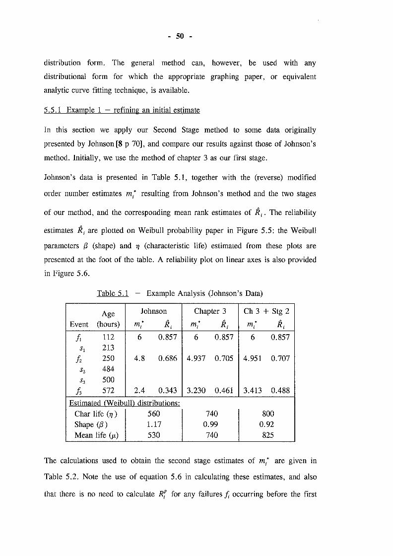
- 50 -

distribution form. The general method can, however, be used with any

distributional form for which the appropriate graphing paper, or equivalent

analytic curve fitting technique, is available.

5.5.1 Example 1 -refining an initial estimate

In this section we apply our Second Stage method to some data originally

presented by Johnson [8 p 70], and compare our results against those of Johnson's

method. Initially, we use the method of chapter 3 as our first stage.

Johnson's data is presented in Table 5.1, together with the (reverse) modified

order number estimates mi* resulting from Johnson's method and the two stages

of our method, and the corresponding mean rank estimates of R i • The reliability

estimates Ri are plotted on Weibull probability paper in Figure 5.5: the Weibull

parameters (3 (shape) and 'iJ (characteristic life) estimated from these plots are

presented at the foot of the table. A reliability plot on linear axes is also provided

in Figure 5.6.

Table 5.1 - Example Analysis (Johnson's Data)

Age Johnson Chapter 3 Ch 3 + Stg 2

Event (hours) m.* I R.i m.*

I R.i m.* I R.i

!t 112 6 0.857 6 0.857 6 0.857

Sr 213

fz 250 4.8 0.686 4.937 0.705 4.951 0.707

Sz 484

s3 500

h 572 2.4 0.343 3.230 0.461 3.413 0.488

Estimated (Weibull) distributions: Char life ('IJ) 560 740 800 Shape ((3) 1.17 0.99 0.92 Mean life (p..) 530 740 825

The calculations used to obtain the second stage estimates of mi* are given in

Table 5.2. Note the use of equation 5.6 in calculating these estimates, and also

that there is no need to calculate R{ for any failures/;_ occurring before the first

- 51 -

Figure 5.5 - Weibull Reliability Plot for Example Data

suspension, nor to calculate Rf for suspensions sj following the final failure.

Event

fz

Table 5.2 - Calculation of Second Stage Estimates

( RP (t) - exp {- (t I 740)0·99

} )

Age (hours)

112 213

250 484

500

572

... ~~~ ....... : ... ~ ... ~.f. .............. ~ ............. ~.~~.~f..J ..... =: .... '!!..~~ ...................... .. kt Rp (E) 1 I Rf :E(1 I Rf) mi* R; 6 0 6 0.857

4

1

0.747

0.711 0.518 0.507

0.461

1.338

1.924 1.971

1.338 4.951 0.707

5.238 3.413 0.488

To show the effects of using a different method for the first stage, we repeat this

example using Johnson's method as the first stage. The second stage calculations

for this variation are presented in Table 5.3. Note that these results are very close

- 52 -

Figure 5.6 - Linear Reliability Plot for Example Data

to those obtained just by using the method of chapter 3. This further illustrates

the consistency of our proposed methods, and also shows that the second stage

method is able to correct the insensitivity of existing methods such as Johnson's.

Event

/1 sl

fz

Sz

s3

h

Table 5.3 - Calculation of Second Stage Estimates

( RP (t) = exp {- (t /530)1. 17} )

Age k.* + [ R{ X El!Rf] - m.* I I ..................................................................................................................................

(hours) k.* I

RP(E) 1/ R~ E(1/ Ri) m.* I R.i

112 6 0 6 0.857 213 0.724 1.381

250 4 0.678 1.381 4.936 0.705 484 0.430 2.324 500 0.417 2.401

572 1 0.359 6.105 3.190 0.456

For both variations of this example, we note that the second stage estimates of

reliability are noticeably larger than the estimates from Johnson's method,

- 53 -

because the second stage method takes account of the increased service of the

suspensions beyond their previous failures, while Johnson's method does not.

5.5.2 Example 2 - demonstration of continuity

To demonstrate the continuity of our second stage method, we return to the

simple example of chapter 2 (section 2.5, Table 2.1) which we used to

demonstrate the discontinuity of existing methods such as Johnson's. The data

from this example is reproduced as Table 5.4, and Table 5.5 presents the mean

rank reliability estimates Ri for stages 1 and 2 in each of these cases. The method

of chapter 3 was again used as the first stage, and equation 5. 6 was used to

calculate the modified order numbers mt for the second stage. The Weibull

parameter estimates quoted were obtained by fitting a straight line through the

points after plotting them on Weibull paper.

Figure 5.7 - Weibull Reliability Plot: Second Example

- 54 -

Table 5.4 - Example Reliability Data (age in hours at failure I suspension)

Event Case 1 Case 2 Case 3 Case 4

fl 100 100 100 100 sl 102 150 198 -

fz 200 200 200 200 (sl) - - - 202

MTBF 201 225 249 251

Table 5.5 - Second Stage Reliability Estimates CRJ for Multiple Cases

Case 1 Case 2 Case 3 Case 4 Event Stg 1 Stg 2 Stg 1 Stg 2 Stg 1 Stg 2 Stg 1 Stg 2

fl 0.75 ~ 0.75 0.75 ! 0.75 0.75 ~ 0.75 0.75 0.75 0.376 ~ ~ 0.498

. fz 0.377 0.417 1 0.431 0.495 0.5 0.5

Estimated CWeibull) distributions: T}: 203 203 217 223 263 265 267 . . (3: 1.76 1.76 1.61 1.55 1.29 1.28 1.27

Figure 5. 8 - Linear Reliability Plot: Second Example

- 55 -

The reliability estimates Ri from the second stage have been plotted (on Weibull

and linear scales respectively) in Figures 5.7 and 5.8, together with the fitted

reliability function estimates. From these results it is quite clear that the estimates

Ri vary continuously as the ages of the suspensions change, and that the same is

true for the estimated reliability functions fitted to these points.

5.6 Summary

In this chapter, we have examined Johnson's concept of modified order numbers

and have developed an alternative expression for calculating these quantities.

Based on this alternative formulation, we have presented two procedures for

calculating modified order numbers, both of which exhibit the desirable

properties of continuous sensitivity to changes in suspension ages. In examining

the conceptual basis for modified order numbers, we have also shown that

Johnson's method of estimating them is only justified in cases where all

suspensions occur at failure events.

Of the two procedures presented in this chapter, the first is equivalent to the

method presented in chapter 3, and does not require any information beyond the

failure and suspension ages of the sample items. By contrast, the second

procedure is a second stage method: it requires the existence of an initial estimate

RP (t) for the reliability function R(t), and provides a method for further refining

that estimate.

We have shown that the second stage procedure presented here is quite tolerant of

inaccuracies in the initial estimate, so that it may be used in conjunction with a

range of initial estimates, including those fitted to existing methods such as

Johnson's. We have also demonstrated - both theoretically and by example

that this method exhibits the desirable continuity properties mentioned above, a

statement which is not true for any of the existing graphical methods of reliability

estimation.

· Chapter 6: Various Extensions of Earlier Results

6.0 Introduction

In this chapter we consider several extensions of the work described in the

previous chapters. All of these are related to our general topic of estimating

reliability levels for items in general multiply censored samples, and all of them

provide estimates that are continuously sensitive to any changes in the ages of

suspended items in the sample concerned.

We discuss firstly a non-parametric reliability estimate based on the method of

chapter 3, which provides a piece-wise linear estimate of reliability for all ages

up to that of the final failure. This estimate makes more apparent the extra

information obtained by the earlier method from the actual ages of suspended

items within the sample.

Secondly, we present a method for obtaining indicative reliability estimates at

ages beyond that of the final failure in the sample. This method provides direct

estimates of reliability levels, based on the information provided by the ages of

the suspended items in this region. No such estimates have been found in the

existing literature.

Thirdly, all reliability estimates have a degree of uncertainty associated with

them, with greater uncertainty accompanying the estimates derived from smaller

samples. We consider the current practice for indicating this uncertainty and

present a variation that is more realistic for heavily censored samples. This

variation reflects our argument that the occurrence of suspensions reduces the

effective size of the sample on trial.

Fourthly, we present a variation of the Kaplan-Meier step-function estimate that

is continuously sensitive to changes in suspension timings, and we also provide

an alternative step-function form which provides a ready comparison between the

original sample size and the current sample size in progressively censored

samples.

- 57 -

6.1 Non-Parametric Reliability Estimation

The method of chapter 3 provides a set of point reliability estimates R i that are

continuously sensitive to changes in suspension ages. The motivation and diagram

that were used to justify this method can also be adapted to provide a continuous

estimate of the reliability function R(t) 1• The resulting estimate retains the

property of continuous sensitivity to changes in suspension timings, and provides

a non-parametric estimate for the reliability function. We consider this estimate

and its properties below.

6.1.1 Description of method

Figure 6.1 - Graphical Representation for Suspensions Mid-Interval

Figure 3.2 (reproduced here as Figure 6.1) was used to justify our estimates of

reliability at certain specific ages, viz. the observed failure events in the sample.

We note that this diagram also indicates an explicit reliability estimate at each

1. This suggestion is due to my supervisor, Professor Nicholas Hastings.

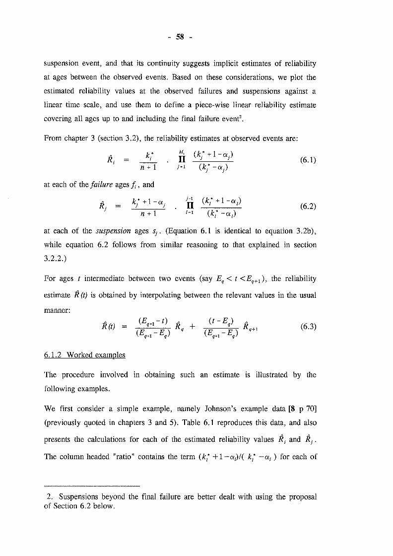
- 58 -

suspension event, and that its continuity suggests implicit estimates of reliability

at ages between the observed events. Based on these considerations, we plot the

estimated reliability values at the observed failures and suspensions against a

linear time scale, and use them to define a piece-wise linear reliability estimate

covering all ages up to and including the final failure event2.

From chapter 3 (section 3.2), the reliability estimates at observed events are:

k.* I

n+1

at each of the failure ages :h , and

It (k/ + 1-a)

i=1 (k/ -a)

j-1 (k * 1 ) n l + -al

1=1 (kt -az)

(6.1)

(6.2)

at each of the suspension ages si. (Equation 6.1 is identical to equation 3.2b),

while equation 6.2 follows from similar reasoning to that explained in section

3.2.2.)

For ages t intermediate between two events (say Eq < t <Eq+1 ), the reliability

estimate R (t) is obtained by interpolating between the relevant values in the usual

manner:

R(t) -(t- Eq) R

(E -E) q+t q+l q

(6.3)

6.1.2 Worked examples

The procedure involved m obtaining such an estimate is illustrated by the

following examples.

We first consider a simple example, namely Johnson's example data [8 p 70]

(previously quoted in chapters 3 and 5). Table 6.1 reproduces this data, and also

presents the calculations for each of the estimated reliability values R i and R i .

The column headed "ratio" contains the term (k/ + 1-a1)/( kt -a1 ) for each of

2. Suspensions beyond the final failure are better dealt with using the proposal of Section 6.2 below.

- 59 -

the suspensions s1 , and the column headed "IFrevn contains the progressive

product of these terms up to Mi or j -1, as appropriate. The resulting reliability

estimates are plotted as Figure 6.2.

Table 6.1 - Application of Method to Johnson's Example Data

Event Age k* 1-cxj ratio wrev R h 112 6 - - 1 0.857

sl 213 5 .268 1.234 1 0.753

fz 250 4 - - 1.234 0.705

Sz 484 3 .273 1.440 1.234 0.577

s3 500 2 .224 1.817 1.777 0.565

h 572 1 - - 3.230 0.461

Figure 6.2 - Non-Parametric Estimate for Johnson's Example Data

Next, we consider a more complex example, based on the randomly simulated

Weibull data of Table 6.2. The calculations and results are again tabulated and

plotted (Figure 6.3), demonstrating the ease of estimation and the straightforward

nature of the resulting estimate for the reliability function R(t) . The continuity of

the estimated reliability function is also shown clearly.

- 60 -

Table 6.2 - Application of Method to Simulated Example Data

Event Age

!t 40 s1 54 S2 110

156 166 251 660 713 941 1007

k* 1 - Ol; ratio wrev

10 - - 1 0.909 0.899 0.854

9 .889 1.113 1 8 .444 1.134 1.113 7 .079 6 -5 .828 4 3 .847 2 .190 1

1.164

1.207

1.351 1.840

1.262 0.812 1.470 0.802 1.470 ~ 0. 779

1.774 l 0.645

1.774 l

!:!~~ I 0.620 0.477 0.401

Figure 6.3 - Non-Parametric Estimate for Simulated Example Data

6.1.3 Properties of the estimate

Again, these properties are apparent from our derivation and example above, and

are verified formally below.

Proposition: The reliability estimates presented in equations 6.1 and 6.2 have the

- 61 -

following properties:

a. they are sensitive to changes in suspension ages, with increased

service life for a suspended item resulting in increased reliability

estimates for subsequent failures and suspensions;

b. they do not jump discontinuously when suspension ages change

from just before to just after a nearby failure event.

Proof: The proposition has already been proved (in section 3.3) for the estimates

R.i of equation 6.1. The justifications for Rj (equation 6.2) are similar:

First, consider the effect of varying one of the ages s1 in equation 6.2.

Provided that s1 < sj , an increase in any a1 increases the corresponding factor in

the product, and hence increases Rj; this verifies statement (a).

To verify statement (b), suppose that s1 = Eq <h.= Eq+t < sj. As s1 -h. a1 - 1, and so the l-th factor in the product of equation 6.2 approaches

kt l(kt -1) = q* l(q* -1). But if s1 =h., then s1 becomes Eq+t and a1 = 0, so

the ratio now takes the value (kt+1)1kz* ={(q+1)*+1}/(q+1)*

= q*l(q* -1), which is the same value as before. It follows that Rj is continuous

as s1 passes h. , as required. [Q,EDJ

Corollary: From equation 6.3, the reliability estimate R (t) at any age t is a

continuous function of the estimates at ages Eq and Eq+t. The properties (a) and

(b) therefore apply to the general estimates R (t) as well.

6.2 Extending Reliability Estimates Beyond the Final Failure

None of the graphical methods described in chapters 2 to 5 provides direct

estimates of reliability for ages beyond that of the final failure in the sample

being analysed. In practice, many samples have a large proportion of items

lasting beyond the final failure, and these items can often provide further

information on the behaviour of the reliability function in this region.

Our aim in this section is to provide some indication of the reliability levels

- 62 -

applying in this region. By considering the information that is known about the

suspensions in this region, and also by considering the possible outcomes of

leaving those items in service, we obtain a set of "next failure" estimates that

achieves this aim. We also consider the limitations implied by our method of

derivation.

The reliability estimates we describe here will clearly be most useful in the case

where suspensions are observed well beyond the final failure event; such a

situation is not uncommon when considering samples with a low proportion of

failures, eg. data on warranty failures. In fact, by extending the estimation of

reliability levels into this "survival" region, we provide a means of identifying

potentially encouraging departures of the data from the reliability function that

would otherwise be fitted.

6.2.1 Limitations of current graphical methods

The extension that we propose here can be applied to any graphically-based

method of reliability estimation, including the existing methods described in

chapter 2 and the methods we have proposed in chapters 3 to 5. In the situation

where some suspensions outlast the final failure, all of these methods provide

reliability estimates at ages up to the last failure event, but none of them can

proceed any further3 because (in terms of item failures) nothing more happens

beyond this point.

To put this argument another way, whichever of these methods we use, it cannot

take full account of any suspensions which outlast the final failure: such

suspensions do contribute to the analysis by their survival to that age, but any

survival beyond that age is ignored because there is no following failure for it to

affect. The longer these items last, however, the more reliable we would expect

the item to be in this age region, so it seems that we are ignoring some

potentially useful information.

3. These remarks include the Kaplan-Meier estimate, which is undefined beyond the final failure in this situation. They also apply to the method of section 6.1, because the necessary proportions cxj cannot be calculated without a finite value for the age corresponding to the next failure.

- 63 -

In order to proceed further, we consider some hypothetical situations, ie. what

might have happened if the survivors had continued in service for a longer time.

Any of the graphical methods discussed above may be used to estimate the

reliability levels applying to these situations, although we would of course

recommend the method of chapter 3 as the most accurate one.

6.2.2 Optimistic and pessimistic envelopes

We consider first two bounding cases: one in which the remaining survivors

continue to survive indefinitely, and one in which all of them would have failed

"immediately" (ie, at the recorded suspension ages) if they had not been

removed. It is clear that the first bound is unduly optimistic and the second

unduly pessimistic, but we cannot tell by how much in either case without further

knowledge about the actual or expected ages of future failures. In the absence of

such knowledge, these limiting cases provide the best available bounds on the

reliability estimates.

The solutions to these bounding cases are quite straightforward, and are sketched

Figure 6.4 - Extended Kaplan-Meier Reliability Estimates

- 64 -

in Figures 6.4 and 6.5 for the examples presented there. (See later for details of

these examples.) If no further failures occurred, the estimated reliability levels

could drop no further than the value at the final failure and the reliability function

must therefore continue horizontally from that point. Conversely, if all survivors

failed immediately beyond their recorded suspension ages, the reliability estimates

would drop steadily as each of these events was passed.

These two sets of estimates provide upper and lower bounds for the estimated

values of reliability in this "survival" region.

Figure 6.5 - Extended "Chapter 3" Reliability Estimates

6.2.3 The "next failure" estimates

We can obtain a more realistic set of estimates for the reliability levels in the

survival region by considering the question: "What if just one of the surviving

suspensions had been about to fail?" To estimate the reliability in this case, we

would treat that particular suspension as a failure which occurred at the recorded

suspension age, we would leave the other suspensions unchanged, and we would

- 65 -

calculate a reliability estimate for the hypothetical failure. We could then plot this

estimated reliability at the recorded suspension age for the item concerned.

The specific formula used to calculate this estimate will naturally depend on the

estimation method being used. All methods will take into account the existence of

any suspensions between the final actual failure and the hypothetical failure, but

only the methods of chapters 3 to 5 will take full account of the ages of any such

suspensions.

By considering each of the surviving suspensiOns in turn we can generate an

estimate of reliability corresponding to each one; together, these estimates

constitute the desired set of reliability estimates. We denote these estimates as the

set of "next failure" estimates, because they estimate the set of points at which

the next failure would have been plotted if the surviving items had remained in

service until a further failure occurred. We demonstrate the calculation of these

estimates by means of the following example, and then return to consider more

fully their validity and significance.

6.2.4 A numerical example

The data and results for our example are presented in Table 6.3. The data have

been obtained from a simulated Weibull distribution with random censorings.

Table 6.3 - Failure Data and Reliability Estimates

Event Age (hrs)

130

237

336

344

441

actual!" next" failures Event Age

r····················· .. r··················.... (hrs) l K-M l Ch 3

0.857

0.714 . 0.899

0.771

731

846

1113

1304

1342

actual/" next" failures ................................................... . . . .

! K-M ! Ch 3

0.571 0.642

0.429 ! 0.514

0.286j 0.385

0.2;4 i ~:::~

In order to illustrate the general applicability of our extension, the reliability

estimates have been obtained by two different methods, namely the Kaplan-Meier

estimate and the method of chapter 3.

- 66 -

The "next failure" reliability estimates in each case are calculated as follows (see

equation 2.3 and equation 3.2 for the general formulae used here):

(i) if s4 were the next failure, the Kaplan-Meier estimate would drop at this age

to R4 x 2/3 = 0.2857, and the estimate from chapter 3 would be R4 x 3/4

= 0.3853;

(ii) if s5 were the next failure, the estimates would be R4 x 1/2 = 0.2143 and

R4 x (2/4) x (4-cx4)/(3-cx4) = 0.3632, where cx4 = (1113-846)/(1304-846)

= 0.5830;

(iii) if s6 were the next failure, the estimates would be R4 x 0 = 0 and

R4 x(l/4)x{(4-cx4)/(3-cx4)}x{(3-cx5)/(2-cx5)} = 0.3484, where cx4 = 267/496

= 0.5383 and cx5 = 458/496 = 0.9234 .

The extended Kaplan-Meier estimates are plotted as Figure 6.4, while the

estimates from chapter 3 are plotted as Figure 6.5. Note how the set of estimates

plotted in each case gives an indication of the possible values of reliability in the

survival region.

The solid curve on Figure 6.5 is a Weibull distribution with a shape factor ({3) of

1.67 and a characteristic life (rJ) of 1120 hours; this distribution estimate has

been fitted to the actual failures only, by the use of Weibull plotting paper. We

note that two of the three "next failure" points lie noticeably to the right of this

curve, suggesting greater reliability in this region than that predicted by the fitted

distribution. A possible refitted curve ({3 = 1.57, 'YJ = 1200 hours) is shown

dashed on Figure 6.5, as a comparison to the originally fitted curve.

6.2.5 Validity and significance of the "next failure" estimates

We first show that the "next failure" estimates described above are actually

conservative estimates of the reliabilities expected at the next failure.

Consider further what would have happened if all the surviving suspensions had

been allowed to remain in service. In practice we would observe a result

- 67 -

intermediate between the two bounds described above, ie. all the items would fail

eventually but not immediately. Further (ignoring coarseness and rounding of

measurements), no two of the items would fail at identical ages, so there would

always be afirst failure among the group.

Suppose for a moment that we knew which item would fail first, and when this

would occur; we could then calculate and plot a reliability estimate for that event.

The true age at failure would be greater than the recorded (suspension) age of

that item, and the reliability estimate for this event would be greater than or equal

to the "next failure" estimate prescribed by our proposal4• The estimate obtained

in the hypothetical case would therefore be plotted somewhere to the right of (and

possibly above) the estimate we have proposed, thus demonstrating that the latter

is an underestimate (in age, and possibly in reliability) of the "true" reliability

estimate for this event. In this sense our proposed estimate is a conservative

estimate - although it is not possible to say by how much it is conservative.

The second point which needs to be made is that we don't actually know which

of the surviving items will fail next, so that our estimates are best thought of as a

set of realistic (but conservative) candidates for plotting the "next" failure beyond

those recorded. Together, this set of estimates indicate the position of one failure

(whichever of the surviving suspensions would have failed "next"); thus, the

individual estimates in the "next failure" set are not as definitive as the reliability

estimates for the recorded failures - even ignoring the uncertainty about which

age each of these suspensions would fail at. Taken together, however, the set of

estimates does provide an indication of how the reliability levels might behave in

the survival region. Such an indication, based directly on the observed ages of the

items which survived into this region, has not been available before.

6.2.6 Other comments

Some practical points may be made regarding fitting of curves and economy of

4. Equality in this statement applies to the existing estimation methods; the methods proposed by us in earlier chapters yield a higher reliability estimate whenever there are any other surviving items between the final actual failure and the hypothetical failure being considered.

- 68 -

calculations. If there are many suspensions beyond the final failure, one might

choose to calculate and plot the "next failure" reliability estimates for a smaller

subset of these events. Obvious candidates for inclusion in the subset would be

the last suspension and the suspensions immediately adjacent to any noticeable

age gaps in the data.

The following procedure is suggested for fitting a suitable curve to the data:

(1) Fit a reliability function to the failure data in the usual fashion.

(2) Calculate and plot "next failure" estimates for (some of) the suspensiOns

outlasting the final failure.

(3) Compare the new points to the fitted curve: if the extra points lie noticeably

to the right of the fitted curve, it may be appropriate to refit the reliability

function to some combination of the original points and the "next failure" points

(according to judgement!).

6.2. 7 Connection to earlier chapters

The method suggested here represents a similar approach to those of the previous

chapters. We have recommended the method of chapter 3 for calculating the

"next failure" estimates, but even without that link, we note that the extension

proposed here also aims to make maximum use of the information provided by

the survival ages of all suspensions in the sample. Earlier chapters addressed this

issue for suspensions occurring before the final failure, while the method of this

section enables the results to be extended to any later suspension - albeit subject

to greater limitations on the interpretation of the results.

6.3 Conversion to Median Ranks and/or Other Estimates

In this section, we review the relationship between mean rank estimates and other

forms of graphical reliability estimate, particularly the use of 5% and 95% ranks

to provide indications of uncertainty levels applying to the "main" (mean, median

or other) reliability estimates. We first describe the existing practice, then suggest

a more realistic alternative for heavily censored samples.

- 69 -

6.3.1 Large samples with few suspensions

The methods of previous chapters give reliability estimates CR i) at each failure

event in the general (multiply censored) case. These estimates are all extensions

of the mean rank estimates for the uncensored and singly censored cases5•

According to our earlier discussion, these estimates can therefore be converted to

equivalent modified order numbers by using the relationship (equation 5.2;

equation 2.2b) (6.4)

(We have already used this relationship in presenting the results of chapter 3 in

terms of modified order numbers: see equations 3.5 and 3.6.)

If an analyst - perhaps following Johnson's lead - prefers to work with median

ranks rather than mean ranks, he can use equation 2.2c with these modified order

numbers to obtain the desired estimates. In the same way, midpoint estimates

(equation 2.2a) can also be obtained if desired.

Table 6.4 - Example Data from O'Connor (Ref. 1)

Event Age Event Age Event Age Event Age Event Age

st 40 s7 102 sB 150 Szz 158 S31 168

Sz 51 Is 108 !9 153 fto 161 S32 171

!t 54 !6 118 S14 153 Sz3 162 fn 173

fz 70 Ss 128 Sts 153 s24 162 S33 177

s3 73 s9 128 S16 154 Szs 165 S34 181

s4 73 !7 132 Sn 156 Sz6 165 S3s 185

Ss 80 fs 141 Sts 156 Sz7 166 s36 188

h 85 Sw 141 S19 156 Szs 166 !12 200

s6 90 Su 147 Szo 158 Sz9 166 S37 202

~ 96 s12 147 Szt 158 S3o 168 S3s 205

A further use for these order numbers is to provide and plot 5% and 95% rank

estimates [ cf 1 p 69], in order to indicate the uncertainty in the estimated

reliability function obtained from the probability plot. We use an example of

5. See our comments on Herd's and Johnson's methods in Chapter 2; Nelson also justifies his cumulative hazard estimates [10] as s-expected (mean) estimates (but for H(t) rather than R(t)).

- 70 -

O'Connor's [1 p70]6 to illustrate this application of order numbers: the observed

data are reproduced in Table 6.4, the reliability estimates are presented in Table

6.5, and these estimates are plotted as Figure 6.6a. Although there is a noticeable

band of uncertainty about the median rank estimates, this band appears to have

tolerably constant width throughout the sample.

Table 6.5 - Reliability Estimates for Above Example

Event Age m.* l Ro.os Ro.s Ro.95

fl 54 49.994 0.942 0.986 0.999 fz 70 48.952 0.907 0.966 0.992 f, 85 47.865 0.876 0.944 0.982

~ 96 46.737 0.845 0.922 0.969 . is 108 45.583 0.816 0.899 0.954

f6 118 44.414 0.787 0.876 0.938 . f, 132 43.226 0.758 0.852 0.921

fs 141 41.991 0.730 0.828 0.903 f9 153 40.665 0.699 0.801 0.882 flO 161 38.895 0.638 0.766 0.854

fu 173 35.654 0.590 0.702 0.799 f12 200 28.337 0.441 0.556 0.668

6.3.2 Small multiply-censored samples

As discussed in chapter 5, the modified order number mi estimates the average

order number applying to the failure!; if all of the items in the sample had been

allowed to fail, ie. it represents the estimated order number of that failure out of

the original sample of size n . To put this in other words, the process of

estimating the modified order numbers mi seeks to adjust the original order

numbers i while keeping the assumed sample size fixed.

In a similar way, the reverse order number mt estimates the average position of

this item from the end of the sample7 under such conditions, and the process of

estimating mi* adjusts the original reverse ranks ki* while keeping n fixed.

6. Note that the last five values given on p 71 of this reference for the Johnson modified order numbers appear to be incorrect.

7. eg, a reverse order number of 5 indicates the fifth last failure (on average), etc.

- 71 -

Figure 6.6 - Reliability Plots with Confidence Bands: O'Connor's Data

In terms of the actual process involved in conducting the trial, it would be more

realistic to fix the number of items left in service at any given stage (ie, the

- 72 -

reverse rank kt ) and to adjust the notional sample size as items are suspended

from service. Thus, instead of defining mt as (n+ 1)Ri, we would now define ni

(the notional sample size at failure J;) by the relation kt = (ni + 1)Ri, and use

kt and ni instead of mt and n in equation 2.2.

In support of this argument, note that the presence of suspensions in the sample

results in a wider spacing between all subsequent reliability estimates. If one

encountered such wide spacings at the start of an analysis, one would surmise a

smaller sample size than is actually the case, and this would imply a greater

degree of uncertainty about the reliability estimates being calculated. Thus, it is

reasonable to argue that uncertainty bands based on the original sample size are

unrealistically optimistic for those estimates which follow a significant number of

suspensions. By using the current spacing between estimates as a guide, and

taking into account the number of items remaining in service at that stage, one

could hope to obtain a more realistic indication of the appropriate uncertainty

bands.

Based on the method of chapter 3 and noting the arguments above, the defining

formula for ni is

1 = (n +1) kt lmt - 1 (6.5a)

(n + 1) M, (k/ -a) n - 1 ' j=l (k/ + 1-aj)

(6.5b)

where equation 6.5a would be used if Ri or mt had already been calculated, and

equation 6.5b would be used otherwise. (Ri can always be calculated later, if

required, as kt l(ni + 1).)

Under this proposal, there is no difference in the plotted reliability estimates

when mean ranks are used, but there will be some differences in the median

rank, midpoint, and 5% and 95% rank estimates. These differences will be

minimal for large samples with few suspensions, but will be noticeable for

multiply censored samples with comparatively few failures. In particular, the 5%

- 73 -

and 95% confidence bands will become progressively wider as more suspensions

occur, reflecting appropriately the greater uncertainty induced in the results by

"artificially" reducing the size of the sample as the trial progresses.

Table 6.6 - Modified Reliability Estimates for Above Example

Event k.* I nj Ro.os Ro.s Ro.95

fl 48 47.966 0.941 0.986 0.999 fz 47 47.966 0.906 0.966 0.993

h 43 44.816 0.872 0.945 0.983 . h 41 43.740 0.840 0.923 0.972 fs 39 42.635 0.809 0.900 0.958 fc, 38 42.635 0.780 0.877 0.943 f, 35 40.295 0.748 0.853 0.928 . . fs 34 40.295 0.719 0.829 0.910 fg 29 35.370 0.681 0.803 0.896 flO 19 23.913 0.614 0.770 0.887

fll 8 10.443 0.468 0.713 0.892 . . f12 3 4.399 0.225 0.559 0.866

We illustrate these comments by applying our proposal to the previous example.

The values of ni resulting from equation 6.5 are presented in Table 6.6, together

with the corresponding 5%, median, and 95% rank estimates for R at each

failure :h. These reliability estimates are plotted in Figure 6.6b, and indicate a

similar median estimate to the previous analysis, but with wider uncertainty bands

- particularly towards the end of the sample.

In this example, it is unrealistic to treat the final failures as though they occurred

in a sample of size 50: after eleven previous failures, the final failure is one item

among three remaining in service! (Nor is it realistic to treat this as the twelfth

failure out of fourteen, when the conventional estimates give a median reliability

around 0.5.) Under our alternative, the reducing number of items in service has

been acknowledged along with the estimated reliability level, treating (for

example) the final failure as the third last of about 4.4 items. This is a more

realistic estimate of the effective sample size as far as this item and the sample

history are concerned, and results in more realistic uncertainty bands.

- 74 -

6.4 Step Function Reliability Estimates

6.4.1 Direct modification of the Kaplan-Meier estimate

The Kaplan-Meier estimate was described in chapter 2, where we noted that this

estimate (as well as the current point-estimate methods) is insensitive to the

timing of suspension events within the inter-failure intervals. By slightly

modifying the construction used in chapter 3, an improved version of the Kaplan-

Meier method can be derived, in which the estimated reliability levels R (t) are

affected in a continuous manner8 by any changes in suspension ages.

The resulting formula is

= k.*- 1

I

M,

n j=l

(k/ -a) ( k .* - 1 - (¥.)

J J

(6.6) n

where i (as in equations 2.1 and 2.3) is determined by f :::::; t < h+J.

Like the Kaplan-Meier estimate, this formula also reduces to the edf estimate

when there are no suspensions in the data, but it has the advantage in the multiply

censored case of being continuously dependent on variations in the ages of

suspended items. Also, just as the Herd-Johnson estimates can be shown always

to lie within the corresponding steps of the Kaplan-Meier estimate, we note that

the estimates of chapter 3 will always lie within the steps of the estimate given

here.

The application of this formula is demonstrated by the following example. Table

6. 7 presents a set of simulated Weibull data, together with calculations for the

reliability estimates Ri corresponding to each failure f. In this case, "ratio"

refers to the terms (k/ -aj)/(k/ -1-aj) and "IFrevn to the progressive product of

these terms up to the previous event.

8. Note that we are discussing here the effect on R (t) of varying suspension

ages, not the (discontinuous) step-function form of R (t).

- 75 -

Table 6 7 - Continuously Sensitive Alternative to Kaplan-Meier Method

Event Age k*-1 1-a. ]

ratio wrev R. K-M R

St 64 9 .904 1.112 1

Sz 96 8 .856 1.127 1.112

s3 350 7 .475 1.154 1.254

s4 602 6 .097 1.196 1.448 . !t 667 5 - - 1.732 0.866 0.833

Ss 800 4 .432 1.291 1.732 . fz 901 3 - - 2.236 0.671 0.625

A 1041 2 - - 2.236 0.447 0.417 . h 1085 1 - - 2.236 0.224 0.208

Is 1504 0 - - 2.236 0 0

The resulting reliability estimates are plotted beside the usual Kaplan-Meier

estimate in Figure 6. 7. Note the increase in reliability levels for our method over

those estimated by the Kaplan-Meier estimate, due to the extra service recorded

by each of the suspensions beyond its respective previous failure.

Figure 6. 7 - Modified Kaplan-Meier Reliability Plot

6.4.2 A further alternative for step function estimates

Like the original Kaplan-Meier estimate, the reliability estimates of equation 6.6

above take a step-function form, with step heights increasing as the sample size

decreases. An alternative way of indicating the variation in sample size is to

maintain the step height at its original size ( 1/n), and make up any extra "gaps"

- 76 -

in the plot by sloping the lines between the steps. The suggested procedure is as

follows:

(1) Calculate the estimated reliability level /( at each failure/; using the

method of chapter 3.

(2) Calculate the corresponding upper value Ui and lower value Li for

each step using the relationships9 Ui = R.i (n + 1)/ n and Li = Ui - lin.

(3) Plot the values of Ui and Li against the corresponding ages/;, then

join Ro ( = 1) to ul ' Ll to u2' and so on up to the final ui value. Mark

the final Li value (eg, with a right-pointing arrow) to indicate that the

theoretical distribution would be expected to continue to the right.

(4) If desired, mark the mean rank estimate (or other preferred estimate)

R i on each corresponding step.

The example of section 6.4.1 is repeated here, but using the method of this

section. Table 6. 8 presents the reliability estimates R i and the estimated step edge

values Ui and Li; these values are also plotted as Figure 6.8.

Table 6.8 - Calculations for Sloping Step-Function Example

Event Age " Rch3 ui Li

!t 667 0.882 0.970 0.870

fz 901 0.721 0.793 0.693 . . h 1041 0.541 0.595 0.495

~ 1085 0.360 0.396 0.296

Is 1504 0.180 0.198 0.098

Note how the increasing vertical distances between the uniform steps highlights

the decreasing sample size while maintaining a comparison with the original

sample size.

9. These equations reflect exactly the relationships applying between the corresponding quantities in the case of a complete sample. The form given here

disguises the fact that Li satisfies the relationship 1 - Li = (1- R i) (n + 1) In.

- 77 -

Figure 6.8 - "Sloping Step-Function" Reliability Plot

6.5 Summary

In this chapter we have considered several further matters related to the general

topic of estimating item reliability from multiply censored data sets.

Firstly, we have presented a continuous non-parametric reliability estimate, and

we have also proposed a method for extending direct reliability estimates beyond

the final failure in a sample. Both of these extensions recognise - and make full

use of - the information provided by the ages of the suspended items in the

sample.

Secondly, we have suggested a way of allowing more appropriately for the

diminishing size of progressively censored samples, and we have extended the

arguments of earlier chapters to step-function estimates of reliability.

In common with our earlier proposals, all of these methods and proposals provide

estimates which are continuously sensitive to any changes in the ages of

suspended items.

Chapter 7: Summary. Discussion. Suggestions and Conclusions

7.0 Precis

This chapter reviews the material presented in earlier chapters and highlights the

advantages of our improved methods over the existing graphical methods for

reliability estimation. We also make some suggestions about further possibilities

for extending and applying these methods, and present some conclusions

regarding the applicability of our work.

7.1 Summary of Thesis Content

7 .1.1 Review of existing methods

Chapter 2 presents some of the basic concepts and terminology involved in the

estimation of item reliability from sample information, and then describes the

various methods currently used for reliability estimation.

The existing graphical methods, although widely used by reliability analysts, are

inconsistent in their treatment of suspensions occurring near to failure events and

take no account of any service recorded by a suspended item since passing the

age of the previous failure. In other words, these methods are insensitive to most

variations in suspension timings, and their estimates change discontinuously when

a suspension age passes a nearby failure age.

This inconsistency in the existing graphical methods results in reliability estimates

which are pessimistic in the general censored case.

7 .1. 2 Improved graphical methods

In chapters 3 to 5 we present three improved methods of reliability estimation. In

each case we demonstrate - in theory and by examples - that our improved

methods provide realistic reliability estimates which take proper account of the

full service recorded by suspended items.

In terms of the existing methods, the individual improved methods may be

described as follows:

(1) The method of chapter 3 improves Herd's method for failure-censored

- 79 -

samples [7] by extending it to the general multiply censored case. In doing so,

the improved method also extends the mean rank estimates for complete samples.

(2) The method of chapter 4 improves the cumulative hazard estimates proposed

by Nelson [10], providing more accurate mean estimates for the cumulative

hazard function in the general censored case.

(3) The method of chapter 5 improves and corrects Johnson's concept of

modified order numbers [8], and provides a "second stage" method for refining

an initial estimate of the reliability function.

In all cases, the improved methods are justified in the general multiply censored

case, while the existing methods can only be justified in the restricted case of

failure-censored data samples.

7 .1. 3 Further improvements and extensions

Chapter 6 presents several suggestions related to the work of the earlier chapters.

In various ways, these suggestions all continue the theme of obtaining maximum

benefit from the information provided by the sample performance data, and all

are continuously sensitive to variations in suspension timings.

In section 6.1 we presented a continuous estimate for the reliability function up to

the age of the final failure. This estimate is a piece-wise linear non-parametric

estimate, and is obtained by extending the method of chapter 3 to provide

reliability estimates at suspension ages as well as failure ages.

Section 6.2 presents a method for extending graphical methods of reliability

estimation to the region beyond the final failure. In this case, we consider

possible candidates for the "next failure", and use the information provided by

suspensions in this region to provide an indication of reliability levels at these

events.

In section 6.3 we discussed the use of ranks other than mean ranks, including the

use of 5 % and 95 % ranks to indicate uncertainty bands about the estimated

reliability function. We presented an alternative approach to determining these

ranks, based on fixed reverse ranks and a reduction in the effective sample size,

- 80 -

rather than on modifying the order numbers within a fixed sample size. This

approach provides a more realistic indication of the widening uncertainty bands

associated with increasingly suspended samples.

Finally, section 6.4 presents two improvements to the step function reliability

estimate described by Kaplan and Meier [6]. The reliability levels estimated by

the improved methods again take proper account of the full service recorded by

suspended items. The first estimate (section 6.4.1) maintains the "true" (piece­

wise constant) step function form, while the second (section 6.4.2) introduces

sloping lines between steps but retains a fixed step height.

7.2 Significance and Applicability of the Ideas and Methods Presented

We have shown in the course of our arguments that the existing graphical

methods can only be justified in the restricted case of failure-censored data

samples. The more general case of multiply censored data is commonly

encountered in practice, so the demonstrated inconsistencies of the existing

methods are relevant in a large proportion of samples.

By the same argument, the improvements provided by our methods are also

relevant to a large proportion of practical samples. These improvements are

particularly noticeable in small samples and in samples with a large proportion of

suspensiOns.

We have demonstrated in chapters 3 to 5 that the methods of these chapters

provide estimates which are continuously sensitive to changes in suspension ages.

This is the basic property which enables all of them to overcome the identified

inconsistencies in the existing graphical methods. Although we have not

demonstrated this property formally for the step function estimates of section 6.4,

similar arguments can be used to verify the property in this case also.

We have also demonstrated that the methods of chapters 3 and 4 reduce to Herd's

method and Nelson's cumulative hazard estimates (respectively) in the failure­

censored case. Our improved methods thus extend the existing graphical methods

from this restricted case to the general multiply censored case. In practice, they

also correct the existing methods, which are frequently used in the general case

- 81 -

even though they are not justified for that case.

The method presented in section 6.2 provides reliability estimates for suspensions

lasting beyond the age of the final failure. These estimates have been derived by

considering hypothetical failures of these lasting items. We have shown that the

estimates given by this method are conservative, but point out that the set of

estimates together represent a single "next failure". To this extent, these estimates

are less definitive than those for events up to the final failure, but they still

provide useful indications of the expected reliability levels in this region.

Although the extension of section 6.2 can be applied in principle to any graphical

estimation method, we recommend in practice that the methods of chapters 3 or 4

should be used because of their improved accuracy over the existing methods.

The method of section 6.4.1 generalises the Kaplan-Meier estimate in a similar

way to our improvements of other existing methods in earlier chapters. The

resulting estimate retains a feature which is characteristic of the Kaplan-Meier

estimate for censored samples, namely the increasing step heights as further items

are suspended from the sample.

The method of section 6.4.2 provides a slightly different approach for indicating

the reducing number of items remaining on trial. In this method, the step heights

remain constant but the function is allowed to fall between the steps. The purpose

of this approach is to retain in the plot an indication of the original sample size

(which is inversely related to the fixed step height) while still indicating the

"stretching" effect in the reliability estimate due to withdrawing items from the

trial.

7.3 Suggestions for Further Work

7.3.1 Evaluating the impact of these results

As discussed above, the use of our improved graphical methods will generally

result in increased estimates of reliability for multiply censored samples. This has

already been seen in the examples of earlier chapters, and further experience in

applying these methods to a range of data sets should enable the extent of this

- 82 -

improvement to be appreciated and evaluated more fully. Both "real world" data

sets and simulation trials would be useful in this regard.

7.3.2 Dealing with dependent suspensions

When working with censored samples, all estimation methods assume that items

are not deliberately suspended so as to avoid impending failure: this assumption

enables the suspended items to be treated as having an identical failure

distribution to the failed items. Many industrial items, for example those which

are replaced under some form of condition monitoring scheme, cannot therefore

be treated by these methods. A promising alternative is to adapt the method of

chapter 5 by allowing individual distributions to be estimated for the remaining

life of each suspended item1: the reliability estimates generated by the method

would then reflect realistically the actual condition of each suspended item

without being tied to the previous assumption.

7.3.3 Application to goodness-of-fit testing

The field of goodness-of-fit testing deals with formal statistical tests for assessing

consistency between a fitted distribution form and the original sample data.

Although a large body of literature is already available on this subject (see, eg,

12 and its references), concerns have been raised [ eg, 13] about some of the

existing methods. The non-parametric estimates of sections 6.1 and 6.4.1 may

provide a alternative avenue for further exploration within this field.

The following comments indicate a possible basis for this proposal:

(1) The well-known Kolmogorov-Smirnov test is essentially based on comparing

a fitted distribution against the non-parametric Kaplan-Meier (step-function)

reliability estimate.

(2) Harter [5 p 1623] cites a test for complete samples that is similar to the

Kolmogorov-Smirnov test, but based instead on comparison with the mean rank

reliability estimates; he comments that this test is more evenly sensitive to

1. For example, such an estimate could be based on the opinion of an experienced repairer who has inspected the item after its removal.

- 83 -

variations at different order numbers than the Kolmogorov-Smirnov test is.

In both of these cases, we see that the goodness-of-fit test is using a non­

parametric estimate of the item reliability as a gauge for testing the proposed

(fitted) parametric distribution. Our suggestion is that the non-parametric

estimates of sections 6.1 or 6.4.1 could be used in similar fashion, and might be

found to provide a test or tests with desirable properties similar to that cited by

Harter. It may also be found that such tests generalise the existing methods

properly to the multiply censored case, just as the methods we have presented in

previous chapters generalise the existing graphical methods for estimating

reliability levels.

The following comments are also relevant:

(3) A test of this sort could conceivably be related to a step-function form

(section 6.4.1), to a point estimate form (eg. chapter 3) or to a continuous form

(section 6.1). In practice, the test statistic would presumably be expressed either

as a maximum deviation from the step-function or point estimate, or as an

averaged (integrated) deviation from the continuous estimate.

(4) In any of these cases, the effect of decreasing sample stze in a censored

sample would need to be taken into account. The approach of section 6.3.2 - or

some generalisation of it - would appear to be relevant to these considerations.

7.4 Conclusions

7 .4.1 Improved reliability estimates

Several variants of the graphical method are commonly used for estimating item

reliability from samples with suspended items. In the general case - viz, unless

the suspensions are restricted to occur only at failure ages - these methods

provide reliability estimates that are consistently pessimistic.

In this thesis we have developed several improved graphical methods, each of

which takes into account the full recorded service of suspended items. Each of

these improved methods reduces to an existing method when justified, but

provides more realistic reliability estimates in the general case.

- 84 -

One or more improved methods have been presented for each of the commonly

used graphical methods, namely for the Kaplan-Meier estimate, the Herd and

Johnson estimates, and Nelson's cumulative hazard estimates. The methods we

have presented are also easily adapted to any similar formulations.

Based on our improvements, we have also presented a continuous non-parametric

estimate for the reliability function.

7.4.2 Extended reliability estimates

It is quite common for samples to contain suspended items which have outlasted

the final recorded failure. In these cases, existing graphical methods are restricted

to providing direct estimates only up to the age of this failure.

This thesis presents a method of providing direct reliability estimates for the

items which outlast the final failure, thus extending the applicability of graphical

estimation methods. This extension has particular application to the analysis of

data in which a large proportion of the sample may have outlasted the final

recorded failure.

7.4.3 Further possibilities

Three possibilities for further work have been suggested. The first involves

further evaluation of our improved methods, the second concerns the prospect of

extending reliability analysis methods to the case of "condition-censored" data,

and the third describes a possible application of our results to the field of

goodness-of-fit testing.

Bibliography

References cited:

1. O'Connor, P.D.T., Practical Reliability Engineering, John Wiley & Sons

Ltd, Chichester (etc), 3rd edition: 1991.

2. Nelson, W., Applied Life Data Analysis, John Wiley & Sons Inc., New York, 1982.

3. D'Agostino, R.B., "Graphical analysis": Chapter 2 (pp7-62) of D'Agostino and Stephens (Ref. 12).

4. Michael, J.R. and Schucany, W.R., "Analysis of data from censored samples": Chapter 11 (pp461-496) of D' Agostino and Stephens (Ref. 12).

5. Harter, H.L., "Another look at plotting positions", Communications in

Statistics - Theory and Methods, v13 (1984), pp1613-1633.

6. Kaplan, E.L. and Meier, P., "Non-parametric estimation from incomplete

observations", Journal of the American Statistical Association, v53 (1958) pp457-481.

7. Herd, G.R., "Estimation of reliability from incomplete data", (Proceedings

of) 6th National Symposium on Reliability and Quality Control (1960) pp202-217.

8. Johnson, L.G., Theory and Technique of Variation Research, Elsevier, Amsterdam (etc), 1964.

9. Johnson, L. G., The Statistical Treatment ofF atigue Experiments, Elsevier,

Amsterdam (etc), 1964.

10. Nelson, W., "Theory and applications of hazard plotting for censored

failure data", Technometrics, v14 (1972), pp945-966.

11. Kapur, K.C. and Lamberson, L.R., Reliability in Engineering Design,

Wiley, 1977.

12. D'Agostino, R.B. and Stephens, M.A., Goodness-of-Fit Techniques

(Vol. 68 in "Statistics: Textbooks and Monographs" series), Marcel

Dekker Inc., New York, 1986.

13. Ang, J.Y.T. and Hastings, N.A.J., "Model accuracy and goodness of fit

for the Weibull distribution with suspended items", Microelectronics

Reliability, v34 ( 1994), pp 1177-1184.

- 86 -

Publications based on the work described in this thesis1:

Hastings, N.A.J. and Bartlett, H.J.G., "Estimating the failure order-number from reliability data with suspended items", IEEE Transactions on

Reliability, v40 (1997), pp266-268.

Bartlett, H.J.G. and Hastings, N.A.J., "Improved reliability estimates for samples containing suspensions", (Proceedings of) 2nd International

Conference on Quality and Reliability (Hong Kong, 1-3 September 1997), v2, pp315-318 (refereed conference).

Bartlett, H.J.G. and Hastings, N.A.J., "Improved reliability estimates for samples containing suspensions", Journal of Quality in Maintenance

Engineering, v40 (1998) n2 (ICQR '97 special issue: Maintenance

Engineering), pp107-114 (revision of ICQR '97 paper).

Hastings, N.A.J. and Bartlett, H.J.G., "Reliability analysis with sensitivity to suspension timings", International Journal of Reliability, Quality and

Safety Engineering, to appear March 1998 (Special Issue: Maintenance

Theory and Applications).

Bartlett, H.J.G. and Hastings, N.A.J., "Continuous reliability estimates for samples containing suspensions", submitted to IEEE Transactions on

Reliability.

1. (Copies of each of these papers follow.)

266 IEEE TRANSACfiONS ON REUABILITY. VOL 46, NO.2, !997 JUNE

Estimating the Failure Order-Number from Reliability Data with Suspended Items

Nicholas A. J. Hastings Queensland University of Technology, Brisbane

Harold J. G. Bartlett , ·Queensland University of Technology, Brisbane ·

Key W~ros·:_ Fail~re, suspension, Order-~~ber.

Summary & Conclusions- A new age-sensitive method (ASM) estimates the order-number of failures in reliability data with suspended items. ASM considers the age of the items at suspen­sion, and is thus more sensitive than methods which consider only the sequence of events. ASM indicates greater reliability in response to increased successful performance data, even when the sequence of failures & suspensions remains unchanged.

1. INTRODUCTION

Acronyms

ASM JM

age-sensitive method (used in this paper) the Johnson method [4: chap 8].

In reliability tests it is common to analyze data relating to some items which have failed and some which have not fail­ed; the latter are callesJ.stispended items, suspensions, or cen­sored items. The data consist of ages at failure & suspension; the aim is to estimate the Cdf as a function of age for the items.

Graphically-based methods are commonly used to estimate this Cdf [1 - 3]. If there are no suspensions, the procedure is common and uses the order-number of each failure (the sequence number of that failure by age); the earliest failure by age has order~.number 1, the second has order-number 2, etc.

If there are suspended items, the widely accepted procedure is described by Johnson [4, 5: pp 37-41], and (somewhat dif­ferently) by Herd [6]. Johnson modifies the order-numbers of the failures to allow for the presence of the suspensions, and then calc_ulates the plotting positions (probability estimates) from these modified numbers. Subsequent texts on reliability engineering, such as Kapur & Lamberson [7: p 316], and O'Connor [8: pp 68-69], use JM.

This paper refines JM for estimating the modified order­number. JM takes no account of the timing of the suspensions in the intervals between failures, whereas our ASM does use the timing of the suspensions in estimating the m;.

An example of this type of data is in Johnson [4: p 70] and is case 1 in table 1.

Notation

fi failure i (ordered by age) fo=O

n

order-number of fi suspension j (ordered by age) modified order-number of fi; 111{) = 0 m;- m;-t event number of fi: i + 'number of suspensions prior to fi' sample size: total number of items on test

m~ I n + 1 - m;; (n+ 1) ·R;, R; is Nelson/Herd reliability

estimate k*; n + 1 - k;; Nelson reverse-rank [1: pp 132, 147] aj (sj -fi-t) I (Ji - fi_ t> ~ 1 - Cij·

Other, standard notation is given in "Information for Readers & Authors'' at the rear of each issue.

2. JOHNSON METHOD FOR m;

JM produces the recursive formula for calculating m; [4: p 74; 7: p 316; 8: p 69]:

Ll; = mj_ 1 I ( kt + 1 ) . (1)

Eq (1) is derived using assumption #HI.

Assumption

H1. From Herd, suspensions occur concurrently with a failure event. 1 ~

Obtain m; by estimating the s-expected total number of failures that would occur if the suspended items were allowed to remain in service until they also failed.

Consider a single suspension which occurs at fi _ 1• If allowed to continue in service, this item could fail before fi, or in any later interval between events, or in the interval follow­ing the final event: a total of ki + 1 intervals. On average, the chances of failing in any of these intervals are equal; m particular,

Pr{failing in [~:::l• fi)} = l!(ki + 1).

Thus, a suspension atfi_ 1 results in:

• ll(ki + 1) s-expected failures in [fi-t> fi), • kif (ki + 1) s-expected survivors at fi.

In general there are:

• r;-1 = k;-1 - m;- 1 s-expected survivors atfi_" • qi-I = k; - k;_ 1 - 1 new suspensions atfi_ 1•

1This assumption is relaxed to derive (3) in section 3.

0018-9529/97$10.00 ©1997 IEEE

RASTmGS/BARTLETI: ESTIMATING FAILURE_ORDER-NUMBER FROM RELIABILITY DATA WITH SUSPENDED ITEMS 267 . . .. ····-. ---...

These ri _ 1 & qi _ 1 items generate:

s-expected failures in [[;_ 1, fi). Therefore (allowing also for the observed fi), the increment in mi is:

= mi-II(ki + 1).

This is the Johnson formula (1).

3. AGE-SENSITIVE METHOD for mi

Remove assumption #Hl. ASM gives:

A·= mi-l I k!"+1

I

k~ a· --~-·B·

kl*·+ 1 jEw; k*+­i aj

(2)

(3)

wi = all j such that there exists an sj where sj E [fi -1> fi).

Consider sj occurring in [fi_ 1, fi). In terms of the argument in section 2, the interval from sj to fi represents only ~ of an equi-probable interval; thus we anticipate that sj generates on­ly ~/ (ki + aj) s-expected failures prior to fi. Under these conditions, qi-l represents all new suspensions in [fi-I> fi), and (2) becomes:

(4)

Rearranging (4) by simple algebra gives (3). We can obtain (1) from (3) as the special case where all .

aj = 0. If mean-rank plotting positions are used, this special case also corresponds to the Herd formula [6: p 204; cf 1: p 147].

4. SENSITIVITY OF ASM TO THE AGE AT SUSPENSION

JM is insensitive to changes in suspension ages, provided that the sequence of events is unchanged; We illustrate the dif­ference between JM & ASM by showing the values of the order­numbers obtained for the 3 sets of data in table 1; case 1 is the Johnson original data. Cases 2 & 3 are similar to case 1, ex­cept that:

• in case 2 the suspensions occur as early as possible without changing the sequence of events,

• in case 3 the suspensions occur as late as possible without changing the sequence of events.

Table 2 shows the modified order-numbers for each set of data, using JM & ASM.

Table 1. Data with Varying Suspension Times but the Same Event Sequence

Event

1 2 3 4 5 6

Table 2.

Failure Number

1 2 3

Ages

Case! Case2 Fail Susp (original) (early)

II 112 112 sl 213 112

h. 250 250

s2 484 250 s3 500 250 ~

h 572 572

Comparison of Modified Order-Numbers

ASM

JM Case 2 Case1 (all cases) (early) (original)

1 1 2.2 2.2 2.063 4.6 4.6 3.929

--~

Case3 (late)

112 249 250 571 571 572

Case 3 (late)

1 2.002 3.507

Table 2 shows that the modified order-numbers resulting from ASM are sensitive to the suspension ages. Specifically, higher estimates of the order-number (and hence lower estimates of reliability) are obtained when there is less performance-data on success:

• Case 2, which has the least successful performance data, gives the highest modified order-numbers,

• Case 3, which has the most successful performance data, gives the lowest modified order-numbers.

JM, since it does not use the suspension times, gives the same modified order-numbers in all cases - and as an­ticipated from the last paragraph of section 3 - these numbers are identical to the ASM estimates for case 2, and higher than the ASM estimates in the other two cases. As judged by this example/ JM is unduly pessimistic in all cases except the failure-censored one. Further, since aj E [0, 1], (2) indicates that the maximum degree of pessimism in using (1) to calculate mi is: qi- tf (ki + 1), ie, (number of suspen­sions involved) · (entire increment each would contribute for that' interval). :

Since JM has been used widely since 1964, it is remarkable that (1) was not refined previously. However, although a citation search on Johnson's work yields many references (including [9, 1 0]), none of them proposes or discusses such refinements.

ACKNOWLEDGMENT

This research was partly supported by MIM Holdings Ltd.

' 68 ' t

REFERENCES

[1] W. Nelson, Applied life Data Analysis, 1982; John Wiley & Sons. [2] R.B. D'Agostino, "Graphical analysis", [11: chapter 2, pp 7-62]. [3] J.R. Michael, W.R. Schucany, "Analysis of data from censored

samples", [11: chapter 11, pp 461-496]. [4] L.G. Johnson, Theory and Technique of Variation Research, 1964;

Elsevier. [5] L.G. Johnson, The Statistical Treatment of Fatigue Experiments, 1964;

Elsevier. . [6] . G.R. Herd, "Estimation of reliability from incomplete data", Proc. 6th

· Nat'l Symp. Reliability and Quality Control, 1960, pp 202-2I7. -[7] K.C. Kapur, L.R. Lamberson, Reliability in Engineering Design, I977;

John Wiley & Sons. [8] · P.D.T. O'Connor, Practical Reliability Engineering (3"d eel), 199I; John·

Wiley & Sons. [9] D.l. Gibbons, L.C. Vance, "A simulation study of estimators for the

2-parameter Weibull distribution", IEEE Trans. Reliability, vol R:30, 198I Apr, pp 61-66.

10] T. Seki, S. Yokoyama, "Simple and robust estimation of the Weibull parameters", Microelectronics & Reliability, vol 33, 1993, pp 45-52.

II] Goodness-ofFitTechniques(R..B. D'Agostino, M.A. Stephens,Edr),I986; Marcel Dekker (vol68 in 'Statistics: Textbooks & Monographs' series).

AUTHORS

>r. Nicholas A.J. Hastings; School of Mechanical, Manufacturing, Medical Eng'g;

IEEE TRANSACTIONS ON RELIABILITY, VOL 46, NO. 2, 1997 JUNE

AUSTRALIA. Internet (e-mail): n.hastings@qut.edu.au

Nkholas Hastings is Mount Isa Mines Professor of Maintenance Engineer­ing at Queensland University of Technology. He graduated from the University of Cambridge (1%I) and obtained his PhD (1971) from the University of Birm­ingham. He is the author of several books and computer packages in reliability, statistics, and related fields, and is active in research, education, and consulting in reliability & maintenance engineering.

Harold J.G. Bartlett; School of Mechanical, Manufacturing, Medical Eng'g; Queensland Univ. of Technology; GPO Box 2434; Brisbane, Queensland 4001 AUSTRALIA. Internet (e-mail): h.bartlett@qut.edu.au

Harry Bartlett is a PhD student and former MIM Scholarship holder at Queensland University of Technology. He graduated from the University of Queensland, with degrees in Mechanical Engineering (I977) and Mathematics (I980), and spent IO years as a mechanical engineer in a large Australian mining company before taking up post-graduate studies. His activities include research and tertiary teaching.

Manuscript TR96-043 received I9% April 10; revised I996 October 24.

Responsible editor: W. Kuo

~eensland Univ. of Technology; GPO Box 2434; Brisbane, Queensland 400I Publisher Item IdentifierS 0018-9529(97)04425-4

UTORIAL PAPERS Physics & Chemistry of Failure TUTORIAL PAPERS Physics & Chemistry of Failure TUTORIAL PAPERS

You Can Help

UTORIAL PAPERS Physics & Chemistry of Failure . TUTORIAL PAPERS Physics & Chemistry of Failure TUTORIAL PAPERS

We are interested in receiving tutorial manuscripts n the specifics of failure mechanisms of materials and of 1bricated parts. (These manuscripts will be refereed.)

The ·manuscript should discuss the physics, the hemistry, the metallurgy, etc of the way things fail. We re NOT inviting tutorials on probability, statistics, nd/or other mathematical procedures & concepts.

It is important to designers, especially at the part 1.on-repairable) level, to know:

What kind of "bad things" to watch out for and to void.

How to eliminate or to mitigate the effects of those bad things".

We want papers with both of the following attributes: Non-mathem.atical discussion of the concepts (Albert

Einstein said that if you can't explain it without the math, then you don't really understand it). The purpose of this part is to help engineers know what questions to ask. • Quantitative discussions of the failure mechanisms

(their causes & results). Any quantitative estimates of effects should give some measure of the uncertainty involved. The purpose of this part is to help engineers make accurate, real predictions about reliability.

For the past several years we have been publishing one such paper in each issue; look at those to get an idea of what we are after..... .,.TR,.

ProceeJings of the yJ International Conference on Quality and Reliability f-3 September 1997 Hong Kong Volume 2, pp. 315-318

IMPROVED RELIABILITY ESTIMATES FOR SAMPLES CONTAINING SUSPENSIONS

H.J.G. Bartletr" and N.A.J. Hastingsa aschool of Mechanical, Manufacturing and Medical Engineering,

Queensland University of Technology, GPO Box 2434, Brisbane, Qld 4001, Australia.

Abstract

A method is presented for obtaining better estimates of reliability levels used in Weibull analysis and related techniques. The method, which is applicable when there are suspended items, overcomes an inherent pessimism and discontinuities which occur in existing methods. The proposed method exhibits continuity with respect to all continuous changes in suspension ages. In particular, the reliability estimates change continuously when a change in age at suspension takes that suspension past a failure event.

1. Introduction

Reliability trials commonly produce some items which have failed and some which have not (yet) failed, the latter being known as suspensions (or censorings). The analyst's aim is to estimate the item's reliability function (or the complement of this, the cumulative probability of failure) from the recorded ages of both failed and suspended items.

A method for estimating the reliability function in such situations was proposed by Herd111 and (in a slightly different form) by Johnson121, and this procedure is widely used !3. 4• 51. The Herd-Johnson method exhibits discontinuities in the reliability estimates if a suspension age is varied marginally so as to pass the age of a failure. The same is also true of other related methods, including Nelson's hazard plots[31 and the Kaplan-Meier product limit estimatel61 •

In this paper we propose a two-stage estimation method which eliminates these discontinuities, thus providing less pessimistic estimates of reliability.

2. Terminology

The estimation methods mentioned above are all examples of plotting-based methods, in which the failure and suspension ages are ordered from smallest to largest and a representative reliability level is assigned to each failure event. The (estimated) reliability function (a curve estimating reliability as a function of the item's age) is then fitted to these points. We denote the (ordered) failure and suspension ages as II, h. ... ;; ... and s1 , s2 .••

sj . . • respectively, the ordered list of all events as E1 , E2 • • • Ek -.. En , and the reliability estimates as R'''; (one for each failure};). (Note that some authors prefer to work in terms of estimated probability levels p"';, where p"'; = 1 - R"'; .) We also define the reverse rank k* corresponding to an event Ek by the relationship k* = n + 1 - k .

If there are no suspensions (a "complete" sample), the order number i is used to calculate the reliability estimate R"';. If there are suspended items, one approach is to modify the order numbers to allow for the presence of the suspensions; the resulting modified order numbers m; are then used as though they applied to failures in a complete sample.

315

.. 316

Analogous to k*, we defme m* = n +I - m.

3. The Herd-Johnson Method

The more commonly used form of this method is presented by Johnsonl21 as a recursive formula for the modified order number; using the notation introduced above, this formula is:

m; = rh;_ 1 + m*;- 1 I (k*; + I) , (1)

with m0 = 0. Herd[ll gave an earlier derivation in terms of expected reliability levels; in our notation, his formula is:

(2)

with R" 0 = 1. The equivalence of these two results can be shown by converting Johnson's m; values to "mean rank" probability estimates

p"; = mJ(n +1), (3a)

or to the equivalent reliability estimates

R"; = I - p"; = m*;l (n +I) . (3b)

Because they are based only on the ranks k, of the failure events, the Herd-Johnson estimates are insensitive to the relative timings of suspensions within the intervals between failures. The underlying reason for this behaviour may be found by examining Herd's derivation, which specifically assumes that all suspensions occur ac failure evencs. Even though most practical data sets do not satisfy this condition, the Herd-Johnson method treats them as though they do, ie. it effectively treats each suspension (no matter how close it may be to the following failure) as though it had occurred at the immediately previous failure.

4. Synopsis of Proposed Method

In the maJOrity of practical cases suspensions occur at times other than failure

times, and we would expect this to affect our reliability estimates. Thus there is scope for improving on the Herd-Johnson method, and we propose an improved procedure below.

In Stage 1 of our procedure, we use an adaptation of Herd's method to provide an initial estimate of the reliability function. This adaptation allows suspensions to occur at times other than failure events and adjusts the reliability estimates (at failures) accordingly, thus avoiding the concerns outlined above. An estimate of the reliability function is then obtained in the usual way.

Stage 2 of our method uses the reliability function resulting from Stage 1 to estimate the s-expected number of failures that would occur in each interval if the suspended items were allowed to remain in service unci/ failure. By adding these estimates to the actual (observed) failures we obtain a set of modified order numbers m;, which reflect the s-expected total number of failures (out of n) at each observed failure event.

5. Proposed Method - Stage 1

The factor k*; I (k*; +I) in Herd's derivation (see equation 2) is dependent on his assumption that all suspensions occur at failure events. By defining the fractions

(4)

(with/; determined by /;_ 1 ::; s1 < /; ), we can generalise Herd's result to include suspensions occurring at any age. (Note that a1 is the fraction of an interval survived by s1 out of the (inter-failure) interval it was suspended in.) The resulting reliability estimates are:

(5)

where RA 0 = 1, k* 0 = n +I, and the product is over all j satisfying f;_ 1 ::; s1 < /;.

This formula has the following properties:

a. it reduces to the Herd-Johnson method as a special case when all suspensions occur at failure events (ie, when all o:i = 0);

b. it is sensitive to changes in suspension ages, with increased service before suspension resulting in increased reliability estimates;

c. its reliability estimates do not jump discontinuously when suspension ages change from just before to just after a nearby failure event.

In particular, note that our formula agrees with the Herd-Johnson result whenever suspensions are restricted only to failure events, but gives higher reliability estimates in all other cases. Hence, it is reasonable to claim that the Herd-Johnson formula under-estimates reliabilities in the latter cases (ie, for most practical data sets). This formula also satisfies our original requirement for a set of estimates that change continuously with suspension age.

The formula of equation 5 thus allows us to produce an initial estimate for the reliability function which takes proper account of the information provided by the timing of suspensions relative to failures. We now proceed to refme this estimate as described below.

6. Stage 2 - Improved Modified Order Numbers

We are now in a position to improve upon Johnson's estimates for the modified order numbers m; . As suggested previously, the adjustment from i to m; can be considered as an estimate of how many failures would have resulted (on average) by time/; from the items suspended prior to that time (if they had actually been allowed to remain in service until failure). This relationship may be expressed by

the formula

(6a)

where piJ is the (estimated) probability of suspension si failing before age /; . (The sum is over all suspensions si for which si < .t . )

It is more convenient for calculation purposes to express the above formula as

(6b)

where riJ = I - piJ is the probability of suspension si surviving beyond /; (if it was suspended before /; ; we may stipulate r iJ = 0 for all sj ;;:::: .t ).

For any given sj and (later) /; the probability riJ may be calculated as a conditional survival probability, namely the probability that the item si survives until age/; given that it has already survived until age si. Using the symbol R(E) to represent the estimated reliability of an item at the age given by event E (and with the usual notation for conditional expressions), we have

Using the (estimated) reliability function obtained from Stage 1, we can now estimate R(E) for the relevant failures and suspensions, and hence obtain our riJ estimates. Substituting these values into equation 6 yields the modified order numbers m; (or m *; ) , and the normal procedures for complete samples may then be followed.

Note that this formulation for Stage 2 retains the properties (b) and (c) that also applied to Stage 1, namely, completely continuous sensitivity to changes in suspension ages. In particular, an increased age at suspension si ( <.t ) results in a higher conditional probability riJ , a larger estimate for m*i (ie, a smaller estimate of m; ), and hence a higher estimated reliability level at .t .

317

• 318 •

7. illustrative Example

Table 1 contains data originally presented by Johnson (l2l p. 70); also tabulated are the comparative reliability estimates R"; obtained from the Herd-Johnson method and from each stage of our method, and the estimated reliability functions fitted to each set of estimates. (The latter were fitted "by hand" using Weibull probability paper.) Note the relative pessimism of the Herd-Johnson values, which results from the way that suspensions are treated by that method.

Table 1. Example analysis

Event Age R" (hrs) H-J Stage 1 Stage 2

fl 112 0.857 0.857 0.857 St 213

fz 250 0.686 0.705 0.707 s2 484 s3 500

f3 572 0.343 0.461 0.488

Estimated CW eibull) distributions:

Char. life (77) 560 740 800 Shape ({3) 1.17 0.99 0.92 Mean life (f.l) 530 740 825

By varying the data somewhat it is also possible to demonstrate the discontinuity in the Herd-Johnson estimates as a suspension moves from one side of a failure to the other. Thus (for example), if s3 increased to 571 hours but other events remained unchanged, then the Herd-Johnson method would give the same reliability estimates as those tabulated; however, if s3 became 573 hours, the Herd­Johnson estimate for R" 3 would jump from 0.343 to 0.457.) This discontinuous behaviour may be contrasted with the gradual change in reliability estimates inherent in the method we have presented.

8. Conclusion

We have proposed a method for estimating the reliability function of items whose reliability

data contains suspended items. This method improves upon the earlier methods of Herd and Johnson (whose results are in wide-spread use), providing reliability estimates which are continuously sensitive to all changes in suspension ages and which make use of the information provided by the ages of the suspended items.

Acknowledgement

This research was partly supported by MIM Holdings Limited.

References

[1] G.R.Herd, "Estimation of reliability from incomplete data", Proc. 6th Nat. Symposium on Reliability and Quality Control, 1960, pp.202-217.

[2] L.G.Johnson, Theory and Technique of Variation Research, Amsterdam (etc), Elsevier, 1964.

[3] W.Nelson, Applied Life Data Analysis, New York, Wiley, 1982.

[ 4] P. D. T. 0 'Connor, Practical Reliability Engineering, Chichester (etc), Wiley, 3rd edition, 1991.

[5] K.C.Kapur and L.R.Lamberson, Reliability in Engineering Design, New York (etc), Wiley, 1977.

[6] E.L.Kaplan and P.Meier, "Non-parametric estimation from incomplete observations", Journal of the American Statistical Association, Vol.53, 1958, pp.457-481.

ltnproved reliability estitnates for satnples

containing suspensions H.]. G. Bartlett and N.A.j. Hastings

School of Mechanical, Manufacturing and Medical Engineering, Queensland University of Technology, Brisbane, Australia.

Journal of Quality in Maintena.nce Engineering, VoL 4 No.2. 1998, pp.107·114, 0 MCB University

Press, 1355-2511

ltnproved reliability estitnates for satnples

• • • contatntng suspensions H.]. G. Bartlett and N.A.]. Hastings

School of Mechanical, Manufacturing and Medical Engineering, Queensland University of Technology, Brisbane, Australia.

Introduction Reliability trials commonly produce some items which have failed and some which have not (yet) failed, the latter being known as suspensions (9r censorings). The analyst's aim is to estimate the item's reliability function (or the complement of this, the cumulative probability of failure) from the recorded ages of both failed and suspended items.

Plotting-based methods- such as the Kaplan-Meier product limit estimate (Kaplan and Meier, 1958), the Herd-Johnson method (Herd, 1960; Johnson, 1964), and Nelson's cumulative hazard plots (Nelson, 1982) - are commonly used for estimating the reliability function in such situations. All of these methods provide reliability estimates that change discontinuously if a suspension age is varied marginally so as to pass the age of a failure.

In this paper we propose a two-stage plotting-based method which behaves continuously in such circumstances, and which provides somewhat more optimistic reliability estimates than those of the Herd-Johnson method.

Terminology In any plotting-based method, a representative reliability level is first assigned to each failure event. The (estimated) reliability function (a curve estimating reliability as a function of the item's age) is then fitted to these points.

In order to assign the reliability estimates to the failure events, the failures and suspensions are first ordered into separate lists by age. We use the symbols ~and s1 to denote the i-th failure and the j-th suspension in their respective lists; the index i commonly referred to as the order number of the failure~· For notational brevity, we shall also use the symbol~ or sj to represent the age at which the corresponding event (failure or suspension) occurred.

We next combine the above lists to obtain an ordered list of all events and use the symbol Ek to denote the k-th event in this list We also define the reverse rank k * corresponding to an event Ek by the relationship k * = n + 1 - k. If Ek is the failure~ we may write k * as k * i; if it is the suspension sj> we may write k * as k *j.

This research was partly supported by MIM Holdings Limited.

Improve( reliabilin estimat~

10~

Journal of Quality in Maintenana Engineering, VoL 4 No. 2, 1998 pp. 107-114, 0 MCB UniversitJ

Press. 1355-251:

JQME 4,2

108

Finally, we denote the reliability estimate corresponding to the failure fi as R'\· (Note, however, that some authors prefer to work in terms of estimated probability levels P"i, where P"; = 1 = R"i).

If there are no suspensions (a complete sample), the order number i is used to calculate the reliability estimate R";· If there are suspended items, Johnson's approach is to modify the order numbers to allow for the presence of the suspensions, and then to use the resulting modified order numbers as

------- though they applied to failures in a complete sample. We denote the modified order number corresponding to the failure fi as mi, and we also define m *i = n + 1- mi.

The Herd-Johnson method In this section, we describe briefly the Herd-Johnson method. This method is widely used (Kapur and Lamberson, 1977; Nelson, 1982; O'Connor, 1991), and is the most similar to our proposal among the existing plotting-based methods.

The more commonly used form of this method is presented by Johnson (1964) as a recursive formula for the modified order number; using the notation introduced above, this formula is:

m; = m;_1 + m*;-1 I (k*; + 1) , (1)

with m0 = 0. Herd (1960) gave an earlier derivation in terms of expected reliability levels; in our notation, his formula is:

K'; = K';_1 . k*; I (k*; + 1) , (2)

with R" 9 = 1. The equivalence of these two results can be shown by converting _Johnsons mi values to "mean rank" probability estimates

or to the equivalent reliability estimates

K'; = 1 - PA; = m*; I (n + 1) .

(3a)

(3b)

Because they are based only on the ranks k*i of the failure events, the Herd­Johnson estimates are sensitive to the relative timings of suspensions within the intervals between failures. The underlying reason for this behaviour may be found by examining Herd's derivation, which specifically assumes that all suspensions occur at failure events. Even though most practical data sets do not satisfy this condition, the Herd-Johnson method treats them as though they do, i.e. it effectively treats each suspension (no matter how close it may be to the following failure) as though it had occurred at the immediately previous failure. The results are that the reliability estimates change only when a suspension age

passes a failure age, and that the estimates therefore change discontinuously under these circumstances.

Synopsis of proposed method In the majority of practical cases suspensions occur at times other than failure times, and we would expect this to affect our reliability estimates. Thus there is scope for improving on the Herd-Johnson method, and we propose an improved

Improve< reliabili~ estimate~

10~ procedure below. -------

In Stage 1 of our procedure, we use an adaptation of Herd's method to provide an initial estimate of the reliability function. This adaptation allows suspensions to occur at times other than failure events and adjusts the reliability estimates (at failures) accordingly, thus avoiding the concerns outlined above. An estimate of the reliability function is then obtained in the usual way.

Stage 2 of our method uses the reliability function resulting from Stage 1 to estimate the s-expected number of failures that would occur in each interval if the suspended items were allowed to remain in service until failure. By adding these estimates to the actual (observed) failures we obtain a set of modified order numbers mi, which reflect the s-expected total number of failures (out of n) at each observed failure event.

Proposed method - stage 1 The factor k*/(k*i + 1) in Herd's derivation (see equation 2) is dependent on his assumption that all suspensions occur at failure events. By defining the fraction

a.i = (si - h-1) I({; - h-1) (4)

(with.fi determined by .fi_1 ::; sj <f), we can generalise Herd's result to include suspensions occurring at any age. (Note that aj is the fraction of an interval survived by sj out of the (inter-failure) interval it was suspended in.) The resulting reliaf>ility estimates are:

k*; n k*. + 1 - ex. RA; = RAi-l . -- . j J "}

k*i-1 k*j - (Xi (5)

where R"0 = 1, k* 0 = n + 1, and the product is over allj satisfyingJ;:_1 ::; sj < /;. This formula has the following properties: t

• It reduces to the Herd-Johnson method as a special case when all suspensions occur at failure events (i.e. when all ~ = 0 ).

• It is sensitive to changes in suspension ages, with increased service before suspension resulting in increased reliability estimates.

• Its reliability estimates do not jump discontinuously when suspension ages change from just before to just after a nearby failure event.

JQME 4,2

In particular, note that our formula agrees with the Herd-Johnson result whenever suspensions are restricted only to failure events, but gives higher reliability estimates in all other cases. Hence, it is reasonable to claim that the Herd-Johnson formula under-estimates reliabilities in the latter cases (i.e. for most practical data sets). This formula also satisfies our original requirement for a set of estimates that change continuously with suspension age.

110 The formula of equation (5) thus allows us to produce an initial estimate for ------- the reliability function which takes proper account of the information provided

by the timing of suspensions relative to failures. We now proceed to refine this estimate as described next.

Stage 2 - improved modified order number We now seek to improve upon Johnson's estimates for the modified order numbers mi. Following Johnson's derivation Gohnson, 1964, ch. 8), we consider what might happen to the items which were suspended in our actual sample if these items had all been allowed to remain in service until failure; in particular, we are interested in how the order numbers of the actual failures would be affected under each possible outcome of our conceptual trial. Our aim is to obtain a set of modified order numbers mi, each of which estimates the average order number (out of n) that the corresponding failurefi would have if all items had failed.

In considering the possible outcomes of our trial, we note that the order number of failure fi would only be affected if an earlier suspension sj were to fail between the ages sj and fi, in which case the order number would increase by 1 for each suspension satisfying this condition. The average contribution to mi (i.e. the average over all possible outcomes) from an individual suspension sj is therefore equal to the probability of this item failing between the ages sj anClfi (assuming that it had remained in service beyond s}.

Denoting this probability as p11, we have

(6a)

where the sum is over all suspensions s. for which sj < ft· If we define rij = 1-Pij as the probability of suspensiOn sj surviving be,r.ond

fi (if left in service), and note that the number of terms in our sum is just k i i, we obtain the more convenient formula

m*. = k*. + E. r .. l I J 1J • (6b)

We note again that r ij is the probability that the item sj survives until age ./;l· given that it has already survived until age sj; in other words it is a conditiona prob­ability (of survival). Using the symbol R(fi\s) to represent this conditional reliability and the symbol R(E) to represent the estimated reliability of an item at the age given by event E, we have

(7)

Using the (estimated) reliability function obtained from Stage 1, we can now estimate R(E) for the relevant failures and suspensions, and hence obtain our r ij estimates. Substituting these values into equation (6) yields the modified order numbers mi (or m *),and the normal procedures for complete samples may then be followed.

Note that this formulation for Stage 2 retains the properties (b) and (c) that also applied to Stage 1, namely, completely continuous sensitivity to changes in

Improve reliabilit estimate

11. suspension ages. In particular, an increased age at suspension sj ( <fJ results in a -----­higher conditional probability r ii' a larger estimate form* i (i.e. a smaller estimate of mi), and hence a higher estimated reliability level atfi.

illustrative example Table I contains data originally presented by Johnson (1964, p. 70); also tabulated are the comparative reliability estimates R". obtained from the Herd­Johnson method and from each stage of our method, and the estimated reliability functions fitted to each set of estimates. (The latter were fitted "by hand" using Weibull probability paper, and are plotted as Figures 1 and 2). Note the relative pessimism of the Herd-Johnson values, which results from the way that suspensions are treated by that method.

Age R" Event (hours) H-J Stage 1 Stage 2

/1 112 0.857 0.857 0.857 sl 213 fz 250 0.686 0.705 0.707 sz 484 s3 500 !3 572 0.343 0.461 0.488

Estimated (Weibull) distributions: Char. life ( 17) 560 740 800 Shape (fJ) 1.17 0.99 0.92 Mean life (J.l) 530 740 825

By varying the data somewhat it is also possible to demonstrate the discontinuity in the Herd-Johnson estimates as a suspension moves from one side of a failure to the other. Thus (for example), if s3 increased to 571 hours but other events remained unchanged, then the Herd-Johnson method would give the same reliability estimates as those tabulated; however, if s3 became 573 hours, the Herd-Johnson estimate for R" 3 would jump from 0.343 to 0.457. This discontinuous behaviour may be contrasted with the gradual change in reliability estimates inherent in the method we have presented.

Table I Example analysi~

JQME 4,2

112

Figure 1. Weibull plot of example data

" " R 1-R

0.1 0.9

----0.4 0.6

0.7 0.3

0.9 0.1

100

Further discussion Maximum likelihood method

200

/

/

(7J)

/ /

/ /

/ /

Key - - - - Johnson

Stage 1

-----Stage 2

500 1000

t (hrs) _ __...,.

The maximum likelihood method is sometimes used as an alternative to plotting-based methods for estimating item reliability from trials containing suspended items, and the results of this method are continuously sensitive to changes in the ages of all events, including suspensions. An essential difference from the plotting-based methods is that one must assume a particular distributional form for the reliability function before using this method; when using plotting-based methods, one may choose to do a non-parametric reliability plot or one may try several forms and see which of them fit the data best. In practice, the maximum likelihood method often gives somewhat different results to those of the existing plotting-based methods, due to their different methods of weighting the observations used; this comment is also true when comparing the maximum likelihood method to the two stage method proposed above. On the other hand, our method displays the same desirable property as the maximum likelihood method of continuous sensitivity to changes in suspension ages, without the restriction of having to choose a distributional form before analysing the data.

i <a:

0.5

" " " " " ~ " " " " ........

........ .........

......... .........

Key ' -----Stage 2 ',

--- Stage1 - - - - Johnson

......

04---~----~--~----~--~----.---~--

0

Sample size considerations

300 600 t (hrs)

For samples with a large number of failures, there tends to be little difference between the reliability estimates generated by any two of the existing plotting­based methods. Similarly, the difference between our method and the existing methods will generally be quite small in such cases. The differences will certainly be more noticeable, however, for samples with a small number of failures as we have shown in the example above. In such cases, our method will invariably provide more optimistic estimates of reliability than the existing methods.

Repeated application of Stage 2 By repeating the application of our Stage 2 method to the improved reliability function, one may proceed to obtain a further refined estimate, and this process may in principle be repeated indefinitely. Our experience with this process is that the third and subsequent stages make only minor changes to the estimated reliability function, and that the process settles down to a final estimate within 3 to 5 revisions at most.

It is also possible to apply the second stage of our method (as many times as desired) to an initial reliability estimate generated by an existing method, e.g. from the Herd-Johnson method. The final estimate in this case is found to be very close to the final estimate resulting from our own Stage 1 estimate. We also

Improved reliability estimat~

113

Figure 2. Linear plot of example

JQME 4,2

114

generally find that our Stage 1 estimate is noticeably closer to the final estimate than are the initial estimates from the existing methods.

These observations together indicate an overall consistency in our method, and also suggest that it provides more appropriate estimates of reliability than the existing methods do.

Conclusion ------- We have proposed a method for estimating the reliability function of items

whose reliability data contain suspended items. This method improves upon the earlier methods of Herd and Johnson (whose results are in widespread use), providing reliability estimates which are continuously sensitive to all changes in suspension ages. The method proposed makes use of the information provided by the ages of the suspended items, and enables the estimated reliability function to be refined as closely as desired.

References Herd, G.R. (1960), "Estimation of reliability from incomplete data", Proceedings of the 6th

National Symposium on Reliability and Quality Control, pp. 202-17. Johnson, L.G. (1964), Theory and Technique of Variation Research, Elsevier, Amsterdam. Kaplan, E.L. and Meier, P. (1958) "Non-parametric estimation from incomplete observations",

journal of the American Statistical Association, Vol. 53, pp. 457-81. Kapur, K.C. and Lamberson, L.R. (1977), Reliability in Engineering Design, Wiley, New York, NY. Nelson, W. (1982), Applied Life Data Analysis, Wiley, New York, NY. O'Connor, P.D.T. (1991), Practical Reliability Engineering, 3rd ed., Wiley, Chichester.

RELIABILITY ANALYSIS WITH SENSITIVITY TO SUSPENSION TIMINGS

NICHOLAS A. J. HASTINGS School of Mechanical, Manufacturing and Medical Engineering,

Queensland University of Technology, GPO Box 2434, Brisbane, Queensland 4001, Australia

E-mail: n.hastings@qut.edu.au

and

HAROLDJ.G.BARTLETT School of Mechanical, Manufacturing and Medical Engineering,

Queensland University of Technology, GPO Box 2434, Brisbane, Queensland 4001, Australia

E-mail: h.banlett@qut. edu.au

Received (September 20, 1996) Revised (March 27, 1997)

A two-stage method is presented for analysing reliability data with suspended items. The method proposed takes account of the ages of the suspended items when calculating plotting positions for the failure events. This sensitivity to suspension timings provides a more precise method than other plotting-based methods currently in use.

Keywords: Reliability; Censored Samples; Hazard Plots; Probability Plots.

1. Introduction

In analysing reliability trials we wish to estimate the cumulative probability of failure for a certain type of item as a function of its age. Plotting methods are commonly used for such analysis, 1•

2 the procedure being quite straightforward in the case when all of the items on trial are observed to fail.

In practice, however, we often wish to analyse data relating to some items which have failed and some which have not failed. The latter are called suspended items, and the data consist of ages at failure and ages at suspension. Several variants of the plotting method have been proposed for this situation,3 but all of these are insensitive to the timings of the suspension events (apart from reflecting which failures they occurred between). The method we present below contrasts with these by being fully sensitive to changes in suspension timing.

We consider first an example which demonstrates the insensitivity of existing methods to suspension timings, and then propose a two-stage method which overcomes these problems. The first stage of our method is a refinement of Nelson's cumulative hazard plots, 2 and the second stage uses the results from the first stage to provide a refinement of Johnson's modified order number method. 4

2. Limited Sensitivity of Current Methods

Existing plotting-based methods are summarised by Michael and Schucany;3 these include the Kaplan-Meier product limit estimate,5 the Herd-Johnson method,6.4 and Nelson's cumulative hazard plots.2 Each of these methods uses only the relative ordering of failures and suspensions to estimate the quantities to be plotted, and none of them takes account of the relative timings of the suspensions between failures.

Table 1 - Example Reliability Data (age in hours at failure I suspension)

Event Group 1 Group 2 Group 3

F1 100 100 100 S1 102 198

F2 200 200 200 (S1) 201

MTBF 134 166 167

To illustrate this, consider the application of Nelson's method to a simple example. Suppose that three groups of three items are tested, with the results shown in Table 1. Given the small differences between the performances of groups 2 and 3 and the much larger difference between the performances of groups 1 and 2, we would intuitively expect the results for groups 2 and 3 to be similar and the results for group 1 to be quite different. According to Nelson's method, however, the results for groups 1 and 2 will be identical, while those for group 3 will differ noticeably from those for group 2. (See Table 2.) The extra service recorded by the suspension in group 2 is not recognised, even though it clearly affects the estimate of mean time between failures (MTBF). The same comment is also true of other existing plotting methods: they consider only the relative ordering of failures and suspensions but not the relative timings of suspensions within each interval between failures.

Table 2- Cumulative Hazard Values(%) (Nelson's method)

Event

F1 F2

Group 1

33 133

3. Stage 1 -Alternative Hazard Plots

Group 2

33 133

Group 3

33 83

For the first stage of our analysis, we propose the following alternative to Nelson's method (cf. Nelson2 p132-4; steps 1, 5 and 6 are unchanged, but are included for completeness):

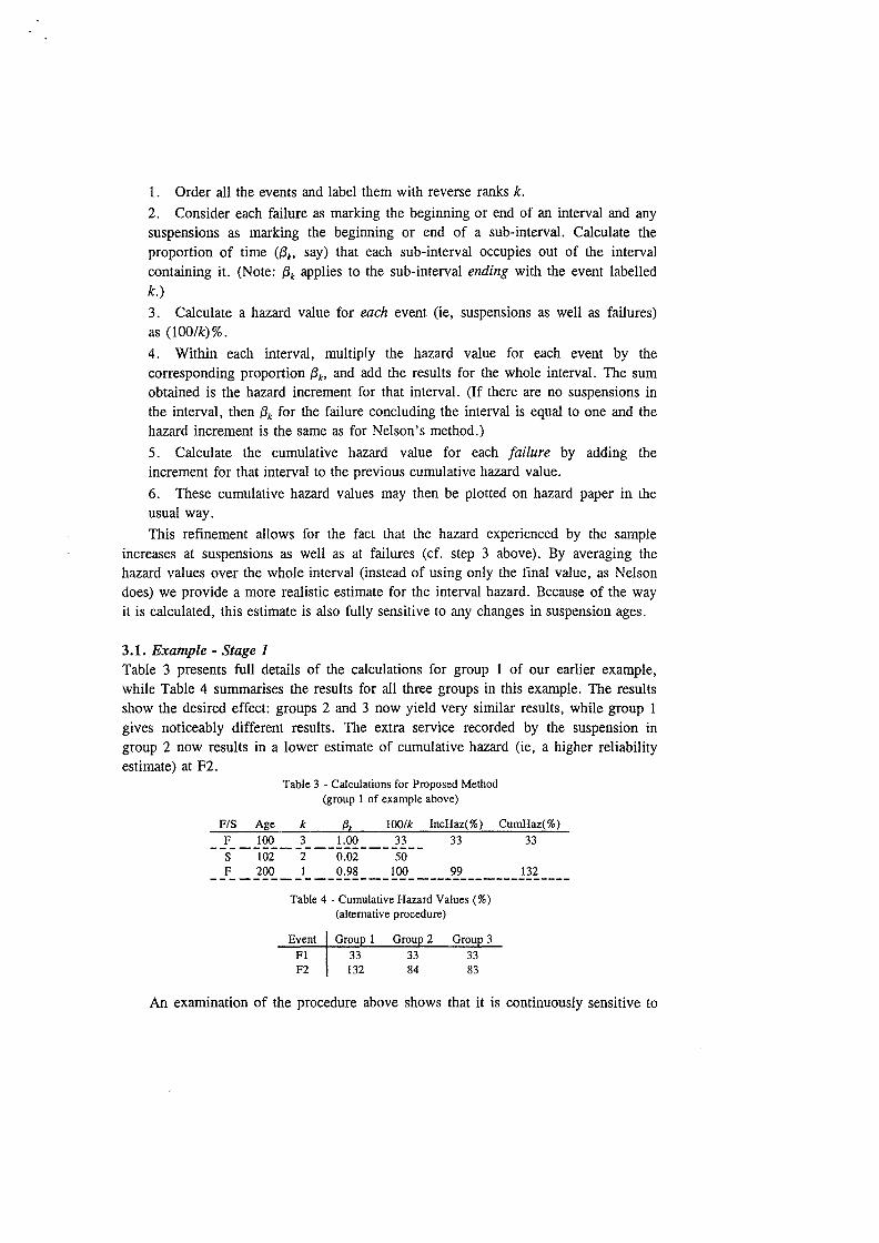
1. Order all the events and label them with reverse ranks k.

2. Consider each failure as marking the beginning or end of an interval and any suspensions as marking the beginning or end of a sub-interval. Calculate the proportion of time (f3k, say) that each sub-interval occupies out of the interval containing it. (Note: f3k applies to the sub-interval ending with the event labelled k.)

3. Calculate a hazard value for each event (ie, suspensions as well as failures) as (100/k)%.

4. Within each interval, multiply the hazard value for each event by the corresponding proportion f3k, and add the results for the whole interval. The sum obtained is the hazard increment for that interval. (If there are no suspensions in the interval, then f3k for the failure concluding the interval is equal to one and the hazard increment is the same as for Nelson's method.)

5. Calculate the cumulative hazard value for each failure by adding the increment for that interval to the previous cumulative hazard value.

6. These cumulative hazard values may then be plotted on hazard paper in the usual way.

This refinement allows for the fact that the hazard experienced by the sample increases at suspensions as well as at failures (cf. step 3 above). By averaging the hazard values over the whole interval (instead of using only the final value, as Nelson does) we provide a more realistic estimate for the interval hazard. Because of the way it is calculated, this estimate is also fully sensitive to any changes in suspension ages.

3.1. Example -Stage 1 Table 3 presents full details of the calculations for group 1 of our earlier example, while Table 4 summarises the results for all three groups in this example. The results show the desired effect: groups 2 and 3 now yield very similar results, while group 1 gives noticeably different results. The extra service recorded by the suspension in group 2 now results in a lower estimate of cumulative hazard (ie, a higher reliability estimate) at F2.

F/S Age

F 100

Table 3 - Calculations for Proposed Method (group I of example above)

k {Jl 100/k IncHaz(%)

3 1.00 33 33 ----------------------s 102 F 200

2 o.oz 50 0.98 100 99

Table 4- Cumulative Hazard Values(%) (alternative procedure)

3 F1 33 F2 132

CumHaz(%)

33

132

An examination of the procedure above shows that it is continuously sensitive to

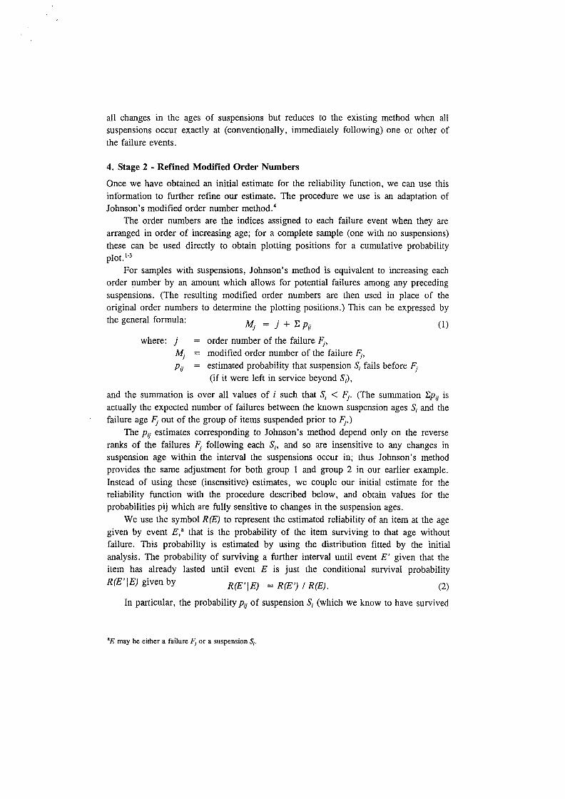
all changes in the ages of suspensions but reduces to the existing method when all suspensions occur exactly at (conventionally, immediately following) one or other of the failure events.

4. Stage 2- Refined Modified Order Numbers

Once we have obtained an initial estimate for the reliability function, we can use this information to further refine our estimate. The procedure we use is an adaptation of Johnson's modified order number method. 4

The order numbers are the indices assigned to each failure event when they are arranged in order of increasing age; for a complete sample (one with no suspensions) these can be used directly to obtain plotting positions for a cumulative probability plot.I-3

For samples with suspensions, Johnson's method is equivalent to increasing each order number by an amount which allows for potential failures among any preceding suspensions. (The resulting modified order numbers are then used in place of the original order numbers to determine the plotting positions.) This can be expressed by the general formula:

where: j

Mj pij

~ = j + Epif

order number of the failure Fj, modified order number of the failure Fj, estimated probability that suspension S; fails before Fj (if it were left in service beyond S;),

(1)

and the summation is over all values of i such that S; < Fj. (The summation Epif is actually the expected number of failures between the known suspension ages S; and the failure age Fj out of the group of items suspended prior to Fj.)

The pij estimates corresponding to Johnson's method depend only on the reverse ranks of the failures Fj following each S;, and so are insensitive to any changes in suspension age within the interval the suspensions occur in; thus Johnson's method provides the same adjustment for both group 1 and group 2 in our earlier example. Instead of using these (insensitive) estimates, we couple our initial estimate for the reliability function with the procedure described below, and obtain values for the probabilities pij which are fully sensitive to changes in the suspension ages.

We use the symbol R(E) to represent the estimated reliability of an item at the age given by event E, • that is the probability of the item surviving to that age without failure. This probability is estimated by using the distribution fitted by the initial analysis. The probability of surviving a further interval until event E' given that the item has already lasted until event E is just the conditional survival probability R(E'\E) given by R(E'\E) = R(E') I R(E). (2)

In particular, the probability pij of suspensionS; (which we know to have survived

•E may be either a failure Fj or a suspension S1•

until age S;) failing between then and failure Fj is found to be

pif = 1 - R(FjiSJ = 1 - R(Fj) I R(SJ. (3)

By substituting these values into (1), we obtain the required modified order numbers Mj.

As with Stage 1, an increase in suspension age indicates greater overall reliability (a longer-lasting S; results in a smaller pif, hence decreasing ~). and the estimates (in this case, M) are continuously sensitive to the changes in suspension ages. We again contrast this proposal with Johnson's method, which is unaffected by such changes unless the order of failures and suspensions is altered.

4.1. Example~ Stage 2

Consider again the example given in Table 1, and suppose that our initial estimate of the reliability function is a Weibull distribution with a characteristic life (17) of 230 hours and a shape factor ({3) of 1.6 . (For the purposes of this demonstration, we ignore the fact that the different groups would actually yield different initial estimates.) For group 1, we have R(F;} = exp{ -(2001230)"1.6} = 0.4495, and R(S1)

= exp{ -(1021230)"1.6} = 0.7617; therefore p12 = 1 - 0.4495 I 0.7617 = 0.41, and hence the value of M2 is 2.41. For group 2, the corresponding values are R(Fz} = 0.4495, R(S1) = 0.4553, p 12 = 0.01, and hence M2 = 2.01 . The greater satisfactory service of the items in group 2 is reflected in the lower value of M2 for this group, and will result in a corresponding increase in estimated reliability (as plotted) at F2.

5. Conclusion

A two stage method has been presented for analysing reliability data with suspended items. The method uses information regarding the suspension times to improve the accuracy of the quantities estimated in the analysis. Other commonly used plotting methods (eg. probability plots based on Johnson's modified order numbers, and cumulative hazard plots) do not provide comparable sensitivity to the timing of the suspension events.

The first stage of our method uses a refinement of Nelson's cumulative hazard plots to provide a preliminary estimate of the reliability function for these items. The second stage combines this preliminary estimate with a refinement of Johnson's modified order number method, to obtain a more accurate estimate of the reliability function.

Acknowledgement

This research was partly supported by MIM Holdings Limited.

References

l. R. B. D'Agostino, in Goodness-of-Fit Techniques, ed. R. B. D'Agostino and M. A. Stephens (Dekker, New York, 1986), p. 7.

2. W. Nelson, Applied Life Data Analysis (Wiley, New York, 1982). 3. J. R. Michael and W. R. Schucany, in Goodness-of-Fit Techniques, ed. R. B. D'Agostino

and M. A. Stephens (Dekker, New York, 1986), p. 461. 4. L. G. Johnson, Theory and Technique of Variation Research (Elsevier, Amsterdam, 1964). 5. E. L. Kaplan and P. Meier, J. Amer. Statist. Assoc. 53, 457 (1958). 6. G. R. Herd, in Proc. 6th Nat'[ Symp. on Reliability and Quality Control (1960), p. 202.

Draft Copy (ieee98.doc)

Harold J. G. Bartlett

Continuous Reliability Estimates for

Samples Containing Suspensions

Queensland University of Technology, Brisbane,

Nicholas A. J. Hastings

Queensland University of Technology, Brisbane,

Key Words - Failure, suspension, reliability, continuous.

Wed 18/2/98

Summary and Conclusions - A method is presented for estimating reliability

levels appropriate to failure events from data containing suspended items. The method

proposed is continuously sensitive to local variations in ages at suspension, even when a

change in age at suspension takes that suspension past a nearby failure event. The method

has advantages over existing methods in which discontinuities occur and which are

inherently pessimistic.

1. INTRODUCTION

Acronyms

ASM age-sensitive method [6]

CAM continuous age-sensitive method (used in this paper)

HJ the Herd-Johnson method [1, 2]

Reliability trials commonly produce some items which have failed and some which

Draft Copy (ieee98.doc) - 2 - Wed 18/2/98

have not (yet) failed, the latter being known as suspensions (or censorings). The analyst's

aim is to estimate the item's reliability function (or the complement of this, the

cumulative probability of failure) from the recorded ages of both failed and suspended

items.

A method (HJ) for estimating the reliability function was proposed by Herd [1]

and (in a slightly different form) by Johnson [2], and this procedure is widely used [3, 4,

5]. As discussed in an earlier paper [6], HJ takes no account of the timing of the

suspensions in the intervals between failures; as a result of this, it exhibits discontinuities

in the reliability estimates if a suspension age is varied marginally so as to pass the age of

a failure.

In this paper we propose an estimation method which eliminates these

discontinuities, but which still reduces to H-J in appropriate circumstances. It will be

useful to consider Herd's and Johnson's approaches to the problem before developing our

result.

Notation

J; i-th failure (ordered by age)

!o = 0

order number of J;

sj j-th suspension (ordered by age)

k; event number of J; :

i + 'number of suspensions prior to J;'

kj event number of sj

n sample size: total ·number of items on test

Draft Copy (ieee98.doc) - 3 -

k*i n + 1 - ki; Nelson "reverse rank" [3: pp132, 147]

k*0 = n + 1

1 - CX· J

where fi_ 1 s s1 < fi

estimated reliability level at age/;

1") . ('lfi Ji) m1z mm J 1 i-1 s s1 < i

M(i) max(} I fi-1 s s1 < fi )

2. HERD'S AND JOHNSON'S METHODS FOR RAi

Herd based his method on the assumption [ 1: p203]:

H1: all suspensions in the sample occur at failure events.

Wed 18/2/98

In situations where Hl applies, k*i is the number of items remaining in service

beyond failure fi_ 1 and its associated suspensions, and Herd notes that the s-expected

proportion of survivors to fi from those remaining in service beyond fi_ 1 is k*i I (k*i + 1);

hence he derives the formula:

(la)

or (equivalently)

i

RAi = n { k*, 1 ( k*, + 1 ) } . (lb) I= 1

This result is depicted graphically in Figure 1, which we will consider later in

more detail.

Although Johnson [2] makes no stated restriction on suspension times and bases

his method on quite different arguments from Herd's, his results are basically equivalent

Draft Copy (ieee98.doc) - 4 - Wed 18/2/98

to Herd's. (For exact numerical correspondence, one converts Johnson's modified order

numbers m1 to "mean rank" probability estimates p"', = 1 - R"'1 = m1 I (n + 1) [3: p147-

8,cf2].)

Johnson's estimates (like Herd's) are insensitive to the relative timings of

suspensions within the failure intervals. For example, Johnson's method yields the same

result even if one delays the suspensions in Figure 1 (b) until just before the following

failures. (See also the examples below.) In other words, Johnson's results are equivalent

to assuming that all suspensions are concurrent with the preceding failures, and then

applying Herd's method to the adjusted data. The convention that failures notionally

predate any concurrent suspensions is consistent with this view of Johnson's method.

In view of the effective equivalence of the two methods we refer to them jointly as

the Herd-Johnson method (HJ).

3. CONTINUOUS AGE-SENSITIVE METHOD FOR R"'1

In the majority of practical cases suspensions occur at times other than failure

times, and assumption H 1 is therefore invalid. Thus there is scope for improving on HJ,

and we propose below a formula which satisfies the following requirements:

1. it reduces to HJ as a special case when Hl does apply (ie, when all

suspensions occur at failure events);

2. it is sensitive to changes in suspension ages (with increased service

before suspension resulting in increased reliability);

3. its reliability estimates do not jump discontinuously when suspensiOn

ages change from just before to just after a nearby failure event.

The ASM described in our earlier paper [ 6] had properties 1 and 2, but did not

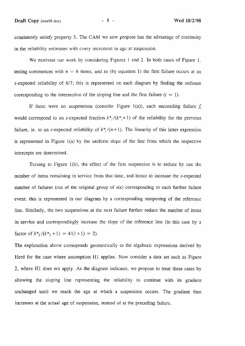
Draft Copy (ieee98.doc) - 5 - Wed 18/2/98

consistently satisfy property 3. The CAM we now propose has the advantage of continuity

in the reliability estimates with every increment in age at suspension.

We motivate our work by considering Figures 1 and 2. In both cases of Figure 1,

testing commences with n = 6 items, and so (by equation 1) the first failure occurs at an

s-expected reliability of 617; this is represented on each diagram by finding the ordinate

corresponding to the intersection of the sloping line and the first failure (i = 1).

If there were no suspensions (consider Figure 1(a)), each succeeding failure J;

would correspond to an s-expected fraction k*i l(k*i+ 1) of the reliability for the previous

failure, ie. to an s-expected reliability of k*)(n+ 1). The linearity of this latter expression

is represented in Figure 1(a) by the uniform slope of the line from which the respective

intercepts are determined.

Turning to Figure 1(b), the effect of the first suspension is to reduce by one the

number of items remaining in service from that time, and hence to increase the s-expected

number of failures (out of the original group of six) corresponding to each further failure

event: this is represented in our diagram by a corresponding steepening of the reference

line. Similarly, the two suspensions at the next failure further reduce the number of items

in service and correspondingly increase the slope of the reference line (in this case by a

factor of k*2 l(k*3 + 1) = 4/(1 + 1) = 2).

The explanation above corresponds geometrically to the algebraic expressions derived by

Herd for the case where assumption Hl applies. Now consider a data set such as Figure

2, where H 1 does not apply. As the diagram indicates, we propose to treat these cases by

allowing the sloping line representing the reliability to continue with its gradient

unchanged until we reach the age at which a suspension occurs. The gradient then

increases at the actual age of suspension, instead of at the preceding failure.

Draft Copy (ieee98.doc) - 6 - Wed 18/2/98

Using the notation defined above, and guided by Figure 2, our general formula

becomes:

(k*, + ' m) M (k*j + ex j) k* ex I

R'". = R"'i-t ------------------ II ----------------- -------------I (2)

k*i-l m+l (k*1_ 1 -ex1_) (k*M-exM)

k* I M (k*j + ex ,J )

= R"'i-t II ---------------- (3a)

k*i-l m ( k*j - exJ )

Equivalently,

k* I

M(i) (k*j + ex'. ) .I

K' = --------- II ----------------I

(3b) n + 1 }=1 ( k* - exJ ) .I

The essential difference between this formula and HJ is that the s-expected number

of failures per interval does not change in CAM until the suspension occurs, whereas HJ

treats the change as occurring at the previous failure - no matter how close the

suspension may actually be to the following failure. A practical consequence of this

difference is that HJ will always under-estimate the reliability function; in the example of

Figure 2, for instance, the HJ estimate of R"'2 takes the value indicated as "b" rather than

the value "a" given by the derivation above.

4. PROOF OF CAM'S PROPERTIES

1. Put ex1 = 0 for j = m, ... M; since k*1_1 = k*1 + 1 (etc), each of the ratios in (2)

is unity except for the final one, which has the value k*)(k*i + 1), as required.

2. Consider equation 3: an increase in any ex1 increases the corresponding factor in

the product and hence increases R"' i·

3. Suppose that sM is the q-th event (£1 ) and/; is Eq+l• and let exM-1 (ie, sM-/;);

the final ratio in (3) then approaches q*l(q* - 1), while the term k*i is equal to

Draft Copy (ieee98.doc) - 7 - Wed 18/2/98

(q + 1)* = q* - 1. Alternatively, if sM =!; then sM becomes Eq+l and!; becomes Eq, so

that the term containing aM disappears from the product, the term k*; becomes q*, and all

other terms remain unchanged: from this it follows that R"; is continuous as sM passes K

A similar argument using the equation for R"l+ 1 shows that reliability estimates at

all later failures are also continuous as sM passes!;.

5. ILLUSTRATIVE EXAMPLES

Table 1 contains data (Case 0) originally presented by Johnson [2 p70], together

with three variations (Cases 1-3) which illustrate the properties of the CAM estimates.

Table 2 (also plotted in Figure 3) presents the calculated reliability estimates from CAM

and HJ. (The curves of Figure 3 have been fitted using Weibull probability plots.) Note

from these results that CAM does indeed satisfy all three of the requirements discussed

above.

Table 1 - Variations of Johnson's Example Data (age in hours at failure I suspension)

Events Case 1 Case 0 Case 2 Case 3

11 112 112 112 112

si 112 213 249 -

12 250 250 250 250

(s I) - - - 250

s2 250 484 571 -

sJ 250 500 571 -

13 572 572 572 572

(s2) - - - 572

(sJ) - - - 572

From these results it is apparent that the reliability estimates resulting from HJ

will jump from the lower curve to the upper curve as the suspensions cross the failure

ages, whereas CAM gives a gradual transition. It also follows that HJ is pessimistic in all

Draft Copy (ieee98.doc) - 8 - Wed 18/2/98

cases except where H1 applies, and our numerical results support this conclusion.

Table 2 - Reliability Estimates by Case and Estimation Method

Case 1 ~ Case 0 Case 2 ~Case 3 Estimate Both HJ CAM HJ CAM~ Both

R''' I 0.857 ~ 0.857 0.857 \ 0.857 0.857 ~ 0.857

R'" 2 0.686 0.686 0.705 0.686 0.7140 0.7143 RA

3 0.343 : 0.343 0.461 : 0.343 0.534 : 0.536

As a further indication of the difference between CAM and HJ, consider a data set

comprising four items, and suppose that one of these items is suspended at some stage. If

we consider the effects on the reliability estimates R'\, R"2 and R" 3 of varying the

suspension age, we obtain the comparison in Figure 4: the reliability estimates are plotted

as functions of suspension age, and clearly contrast the continuous nature of CAM against

the discontinuous results of HJ. (Similar results are also obtained for cases with more

than one suspension, but the plots are more complicated because of the multiple

variables.)

ACKNOWLEDGEMENT

This research was partly supported by MIM Holdings Limited.

REFERENCES

1. G.R. Herd, "Estimation of reliability from incomplete data", Proc. 6th Nat'l Symp.

Reliability and Quality Control, 1960, pp202-217.

2. L.G. Johnson, Theory and Technique of Variation Research, 1964; Elsevier.

3. W. Nelson, Applied Life Data Analysis, 1982; John Wiley & Sons.

4. P.D.T. O'Connor, Practical Reliability Engineering (3rd ed), 1991; John Wiley &

Sons.

Draft Copy (ieee98.doc) - 9 - Wed 18/2/98

5. K.C. Kapur, L.R. Lamberson, Reliability in Engineering Design, 1977; John Wiley

& Sons.

6. N.A.J. Hastings, H.J.G.Bartlett, "Estimating the failure order-number from

reliability data with suspended items", IEEE Trans. Reliability, vol R-46, 1997

Jun, pp266-268.

Figure 1:

Figure 2:

Figure 3:

Figure 4:

List of Captions to Figures

Graphical representation of Herd's formula.

Treatment of data with suspensions mid-interval.

Plot of reliability estimates from Table 2.

Comparison between current proposal and Herd-Johnson method as

suspension age varies.

Draft Copy (ieee98.doc) - 10 - Wed 18/2/98

1

i 6;7

<ct:- %

4;7

%

%

1j7 + + + 0

0 '1 '2 '3 '4 fs fs k*· ,. 6 5 4 3 2 1

Case (a): uncensored

1

i %

<ct:-2•;35

kf: 6 4

Case (b): censored

Figure 1 - Graphical representations of Herd's formula

Draft Copy (ieee98.doc)

1

f R, <at

b.

0

- 11 -

i\ t

I

0 f1 s 1 s2 f2

k*: 4 3 2 1

\

Wed 18/2/98

(notional failure units) ---

Figure 2 - Treatment of data with suspensions mid-interval

Draft Copy (ieee98.doc)

1

0.5

0

0

Figure 3

- 12 -

{ Case 3.·. (both)

::::::: Case 2 (CAM)

Case 0 (CAM)

_ _ _ _ { Cases 0, 2 (HJ)

::::::: Case 1 (both)

300

..... ......

600

.....

t (hrs) ----.

Plot of reliability estimates from Table 2

Wed 18/2/98

Draft Copy (ieee98.doc)

i

0.5

0

0

- 13 - Wed 18/2/98

----- CAM·estimates

- -- HJestimates ·

both estimates

A

R3

-~1 -----_..-==. -- -----=---~----------~

Age at suspension {Item s1 ) -

Figure 4 - Comparison between CAM and HJ estimates as suspension age

varies