Reliability analysis of multilayer multistage

Telecommun SystDOI 10.1007/s11235-015-0093-7

Reliability analysis of multilayer multistage interconnectionnetworks

Fathollah Bistouni1 · Mohsen Jahanshahi2

© Springer Science+Business Media New York 2015

Abstract Multistage interconnection networks (MINs)play a key role in the performance of parallel computers andmultiprocessor systems.A non-negligible demand on today’smodern systems is to deliver multicast traffic. Therefore,design of efficient MINs that meets the routing requirementis vital. One of themain ideas to cope with this problem is theuse of replicated MINs. However, one of the major concernsabout these networks is the problem of unnecessary layerreplication in the first stages, which recently proposes a newidea calledmultilayerMINs. Previous analyzes demonstratedthat this new idea could lead to cost-effective topologiesthat had a very close performance to the replicated MINsin terms of throughput. Also, these analyzes indicate thatthese networks outperform replicatedMINs in terms of delay.However, another critical parameter to prove the performanceof most systems is reliability. Therefore, in this paper, wewill focus on two essential parameters of cost and reliabilityto achieve both objectives; first, evaluating the performanceof multilayer MINs in terms of reliability, second, to findthe best topology among the multilayer MINs introduced inprevious works in terms of cost-effectiveness (mean time tofailure/cost ratio).

Keywords Parallel computers · Multilayer multistageinterconnection network · Reliability block diagrams ·Cost-effectiveness · Mean time to failure

B Mohsen [email protected]; [email protected]

Fathollah [email protected]

1 Young Researchers and Elite Club, Qazvin Branch,Islamic Azad University, Qazvin, Iran

2 Young Researchers and Elite Club, Central Tehran Branch,Islamic Azad University, Tehran, Iran

1 Introduction

A parallel computer requires some kinds of communica-tion subsystems to interconnect processors, memories, andother peripherals [1,2]. In addition, most of the proposalsof switching fabric architectures for asynchronous transfermode (ATM) networks are based on self-routing multi-stage interconnection networks usually known as banyannetworks [3,4]. Furthermore, different proposed intercon-nection topologies for parallel computing have been studiedand adapted for networks-on-chip (NoCs) [5,6]. Therefore,design of an efficient interconnection network is very crucialfor construction of efficient parallel computers and systems-on-chip (SoCs) [2,5–9].

Dynamic interconnection networks include bus, crossbar,and multistage interconnection networks (MINs), which areoften used in the multiprocessor systems [10–12]. The cross-bar networks are the most efficient but the most expensiveones [13,14]. On the other hand, shared bus networks havelower costs but lower performance. MINs provide a com-promise between the above networks because they provideefficient performance using a reasonable number of switches[12,15–20].

Typically, an N×NMIN is constructed by (logc N ) stagesof c × c switching elements and there are

( Nc

)switches per

stage. Therefore, while the crossbar network needs O(N 2

)

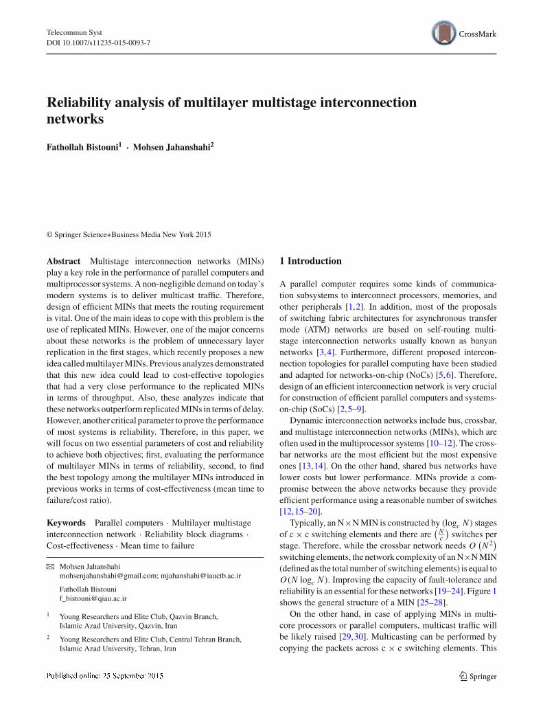
switching elements, the network complexity of anN×NMIN(defined as the total number of switching elements) is equal toO(N logc N ). Improving the capacity of fault-tolerance andreliability is an essential for these networks [19–24]. Figure 1shows the general structure of a MIN [25–28].

On the other hand, in case of applying MINs in multi-core processors or parallel computers, multicast traffic willbe likely raised [29,30]. Multicasting can be performed bycopying the packets across c × c switching elements. This

123

http://crossmark.crossref.org/dialog/?doi=10.1007/s11235-015-0093-7&domain=pdf

F. Bistouni, M. Jahanshahi

Fig. 1 General structure of MINs

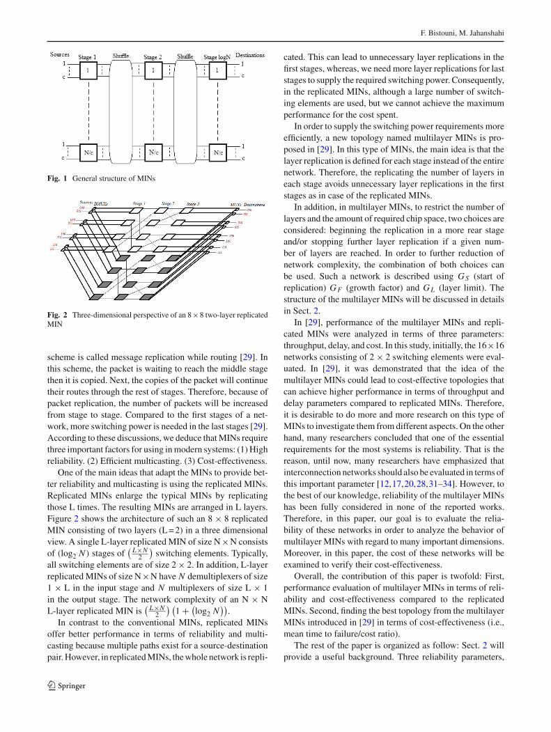
Fig. 2 Three-dimensional perspective of an 8×8 two-layer replicatedMIN

scheme is called message replication while routing [29]. Inthis scheme, the packet is waiting to reach the middle stagethen it is copied. Next, the copies of the packet will continuetheir routes through the rest of stages. Therefore, because ofpacket replication, the number of packets will be increasedfrom stage to stage. Compared to the first stages of a net-work, more switching power is needed in the last stages [29].According to these discussions, we deduce thatMINs requirethree important factors for using inmodern systems: (1) Highreliability. (2) Efficient multicasting. (3) Cost-effectiveness.

One of the main ideas that adapt the MINs to provide bet-ter reliability and multicasting is using the replicated MINs.Replicated MINs enlarge the typical MINs by replicatingthose L times. The resulting MINs are arranged in L layers.Figure 2 shows the architecture of such an 8 × 8 replicatedMIN consisting of two layers (L=2) in a three dimensionalview. A single L-layer replicated MIN of size N×N consistsof (log2 N ) stages of

( L×N2

)switching elements. Typically,

all switching elements are of size 2× 2. In addition, L-layerreplicatedMINs of size N×N have N demultiplexers of size1 × L in the input stage and N multiplexers of size L × 1in the output stage. The network complexity of an N × NL-layer replicated MIN is

( L×N2

) (1 + (

log2 N)).

In contrast to the conventional MINs, replicated MINsoffer better performance in terms of reliability and multi-casting because multiple paths exist for a source-destinationpair.However, in replicatedMINs, thewhole network is repli-

cated. This can lead to unnecessary layer replications in thefirst stages, whereas, we need more layer replications for laststages to supply the required switching power. Consequently,in the replicated MINs, although a large number of switch-ing elements are used, but we cannot achieve the maximumperformance for the cost spent.

In order to supply the switching power requirements moreefficiently, a new topology named multilayer MINs is pro-posed in [29]. In this type of MINs, the main idea is that thelayer replication is defined for each stage instead of the entirenetwork. Therefore, the replicating the number of layers ineach stage avoids unnecessary layer replications in the firststages as in case of the replicated MINs.

In addition, in multilayer MINs, to restrict the number oflayers and the amount of required chip space, two choices areconsidered: beginning the replication in a more rear stageand/or stopping further layer replication if a given num-ber of layers are reached. In order to further reduction ofnetwork complexity, the combination of both choices canbe used. Such a network is described using GS (start ofreplication) GF (growth factor) and GL (layer limit). Thestructure of the multilayer MINs will be discussed in detailsin Sect. 2.

In [29], performance of the multilayer MINs and repli-cated MINs were analyzed in terms of three parameters:throughput, delay, and cost. In this study, initially, the 16×16networks consisting of 2 × 2 switching elements were eval-uated. In [29], it was demonstrated that the idea of themultilayer MINs could lead to cost-effective topologies thatcan achieve higher performance in terms of throughput anddelay parameters compared to replicated MINs. Therefore,it is desirable to do more and more research on this type ofMINs to investigate them from different aspects. On the otherhand, many researchers concluded that one of the essentialrequirements for the most systems is reliability. That is thereason, until now, many researchers have emphasized thatinterconnection networks should also be evaluated in terms ofthis important parameter [12,17,20,28,31–34]. However, tothe best of our knowledge, reliability of the multilayer MINshas been fully considered in none of the reported works.Therefore, in this paper, our goal is to evaluate the relia-bility of these networks in order to analyze the behavior ofmultilayer MINs with regard to many important dimensions.Moreover, in this paper, the cost of these networks will beexamined to verify their cost-effectiveness.

Overall, the contribution of this paper is twofold: First,performance evaluation of multilayer MINs in terms of reli-ability and cost-effectiveness compared to the replicatedMINs. Second, finding the best topology from the multilayerMINs introduced in [29] in terms of cost-effectiveness (i.e.,mean time to failure/cost ratio).

The rest of the paper is organized as follow: Sect. 2 willprovide a useful background. Three reliability parameters,

123

Reliability analysis of multilayer...

terminal, broadcast, and network will be analyzed in Sect. 3.Finally, some conclusions will be derived in Sect. 4.

2 Background

In Sect. 2.1, first, the structure of the multilayer MINs willbe explained in more detail. Then, in Sect. 2.2, related workswithin the context of MINs reliability is presented.

2.1 Structure of multilayer MINs

Following three main factors are defined to describe thestructure of multilayer MINs [29,30]: (1) Start replicationfactor (GS): denotes the stage number at which the replica-tion starts. (2) Growth factor (GF ): denotes the number oflayers which can be developed in a stage by each switchingelement. (3) Layer limit factor (GL): denotes the maximumnumber of layer replication.

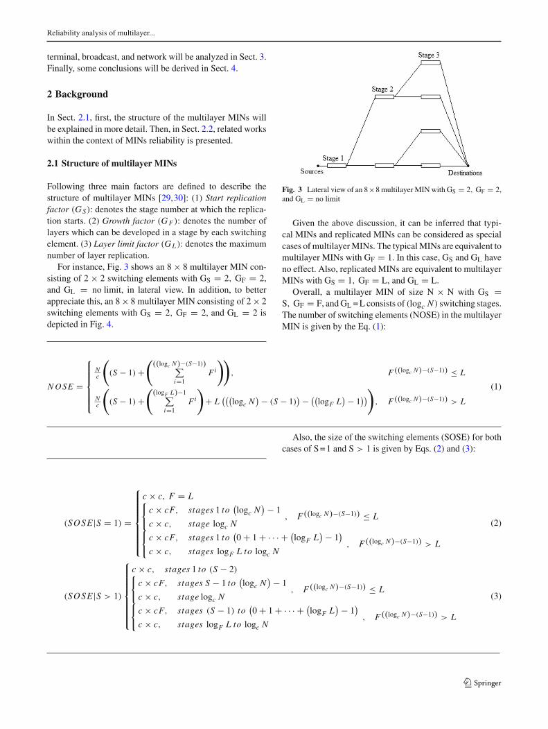
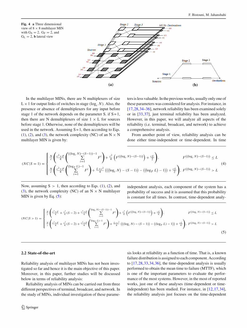
For instance, Fig. 3 shows an 8 × 8 multilayer MIN con-sisting of 2 × 2 switching elements with GS = 2, GF = 2,and GL = no limit, in lateral view. In addition, to betterappreciate this, an 8× 8 multilayer MIN consisting of 2× 2switching elements with GS = 2, GF = 2, and GL = 2 isdepicted in Fig. 4.

Fig. 3 Lateral view of an 8×8 multilayerMINwith GS = 2, GF = 2,and GL = no limit

Given the above discussion, it can be inferred that typi-cal MINs and replicated MINs can be considered as specialcases ofmultilayerMINs. The typicalMINs are equivalent tomultilayer MINs with GF = 1. In this case, GS and GL haveno effect. Also, replicated MINs are equivalent to multilayerMINs with GS = 1, GF = L, and GL = L.

Overall, a multilayer MIN of size N × N with GS =S, GF = F, andGL =L consists of (logc N ) switching stages.The number of switching elements (NOSE) in the multilayerMIN is given by the Eq. (1):

NOSE =

⎧⎪⎪⎪⎪⎨

⎪⎪⎪⎪⎩

Nc

(

(S − 1) +(

((logc N)−(S−1))∑

i=1Fi

))

, F((logc N)−(S−1)) ≤ L

Nc

(

(S − 1) +(

(logF L)−1∑

i=1Fi

)

+ L(((

logc N) − (S − 1)

) − ((logF L

) − 1))

)

, F((logc N)−(S−1)) > L

(1)

Also, the size of the switching elements (SOSE) for bothcases of S=1 and S > 1 is given by Eqs. (2) and (3):

(SOSE |S = 1) =

⎧⎪⎪⎪⎪⎪⎪⎨

⎪⎪⎪⎪⎪⎪⎩

c × c, F = L{c × cF, stages 1 to

(logc N

) − 1

c × c, stage logc N, F((logc N)−(S−1)) ≤ L

{c × cF, stages 1 to

(0 + 1 + · · · + (

logF L) − 1

)

c × c, stages logF L to logc N, F((logc N)−(S−1)) > L

(2)

(SOSE |S > 1)

⎧⎪⎪⎪⎪⎪⎪⎨

⎪⎪⎪⎪⎪⎪⎩

c × c, stages 1 to (S − 2){c × cF, stages S − 1 to

(logc N

) − 1

c × c, stage logc N, F((logc N)−(S−1)) ≤ L

{c × cF, stages (S − 1) to

(0 + 1 + · · · + (

logF L) − 1

)

c × c, stages logF L to logc N, F((logc N)−(S−1)) > L

(3)

123


Fig. 4 a Three dimensionalview of 8 × 8 multilayer MINwith GS = 2, GF = 2, andGL = 2, b lateral view

In the multilayer MINs, there are N multiplexers of sizeL×1 for output links of switches in stage (logc N ). Also, thepresence or absence of demultiplexers for any input beforestage 1 of the network depends on the parameter S. if S=1,then there are N demultiplexers of size 1 × L for sourcesbefore stage 1. Otherwise, none of the demultiplexers will beused in the network. Assuming S=1, then according to Eqs.(1), (2), and (3), the network complexity (NC) of an N × Nmultilayer MIN is given by:

(NC |S = 1) =

⎧⎪⎪⎪⎪⎨

⎪⎪⎪⎪⎩

Nc

(c2×F4

(((logc N)−(S−1))−1∑

i=1Fi

)

+ c24

(F((logc N)−(S−1))

)+ cL

2

)

, F((logc N)−(S−1)) ≤ L

Nc

(c2×F4

((logF L)−1∑

i=1Fi

)

+ L×c24

(((logc N

) − (S − 1)) − ((

logF L) − 1

)) + cL2

)

, F((logc N)−(S−1)) > L

(4)

Now, assuming S > 1, then according to Eqs. (1), (2), and(3), the network complexity (NC) of an N × N multilayerMIN is given by Eq. (5):

(NC|S > 1) =

⎧⎪⎪⎪⎪⎨

⎪⎪⎪⎪⎩

Nc

(c2×F

4 + c24 (S − 2) + c2×F

4

((loge N )−(S−1))−1∑

i=1Fi

)

+ c24

(F((logc N)−(S−1))

)+ cL

4

)

, F((logc N )−(S−1)) ≤ L

Nc

(c2×F

4 + c24 (S − 2) + c2×F

4

((logF L)−1∑

i=1Fi

)

+ L×c24

(((logc N ) − (S − 1)

) − ((logF L) − 1

)) + cL4

)

, F((logc N )−(S−1)) > L

(5)

2.2 State-of-the-art

Reliability analysis of multilayer MINs has not been inves-tigated so far and hence it is the main objective of this paper.Moreover, in this paper, further studies will be discussedbelow in terms of reliability analysis:

Reliability analysis of MINs can be carried out from threedifferent perspectives of terminal, broadcast, and network. Inthe study of MINs, individual investigation of these parame-

ters is less valuable. In the previousworks, usually only oneofthese parameterswas considered for analysis. For instance, in[17,28,34–36], network reliability has been examined solelyor in [33,37], just terminal reliability has been analyzed.However, in this paper, we will analyze all aspects of thereliability (i.e. terminal, broadcast, and network) to achievea comprehensive analysis.

From another point of view, reliability analysis can bedone either time-independent or time-dependent. In time

independent analysis, each component of the system has aprobability of success and it is assumed that this probabilityis constant for all times. In contrast, time-dependent analy-

sis looks at reliability as a function of time. That is, a knownfailure distribution is assigned to each component.Accordingto [17,28,33,34,36], the time-dependent analysis is usuallyperformed to obtain the mean time to failure (MTTF), whichis one of the important parameters to evaluate the perfor-mance of the most systems. However, in the most of reportedworks, just one of these analyses (time-dependent or time-independent) has been studied. For instance, in [12,17,34],the reliability analysis just focuses on the time-dependent

123


analysis, or in [20,31,35,37,38], the reliability analysis onlyfocuses on time-independent analysis. However, this paperwill examine both types of analysis to fully investigate thebehavior of MINs.

In total, given the above discussions, it can be claimed thatreliability analysis are worthwhile in this paper.

3 Reliability and cost

Reliability is defined by the IEEE as the ability of a systemor component to perform its required functions under statedconditions for a specified period of time [39]. Therefore, inthe domain of interconnection networks, many researchershave been convinced that it is the most immediate parameterfor each efficient network [11,20,23,30,33–37].

Complex networks consist of multiple source and des-tination nodes, complex topology, interdependencies at thecomponent and system levels, and uncertainties in actualconditions of network components and deterioration models[40–42]. According to this definition, lifeline networks suchas railway and water distribution networks [40,41,43], wire-lessmobile ad hoc networks (MANETs) [42,44,45], wirelessmesh networks [46–50], wireless sensor networks [51–54],sensors based on nano-wire networks [55], social networks[56], stochastic-flow manufacturing networks (SMNs) [57],and interconnection networks [11,20,23,30,33–38,58–68]are known as complex network systems from the viewpointof reliability.

With regard to the reported researches, reliability inves-tigation of the complex networks can be accomplished bysimulation or analytical models. Although simulation-basedapproaches are easily implemented, there are some restric-tions on their effectiveness. For instance, the statistical natureof simulation models may need a large number of sam-ples to achieve an acceptable level of convergence for verysmall or large probability estimation. In addition, their com-putational efficiency depends on the number of nodes andlinks in a network as they use a path searching algorithmto check the connectivity between the terminal nodes foreach sample. Also, the random number generation processis computationally demanding especially when the compo-nents are statistically correlated as the process includes amatrix decomposition process such as the Cholesky decom-position. Furthermore, simulation presents a small range ofresults compared to the analytical methods. However, sincethe simulation based methods just require the generation ofrandom samples of hazard intensity measures and the cor-responding uncertain status of network components with noneed to identify complex connection system events, analyti-cal methods have been avoided because of their complexityin favor of the simplicity of using simulation. Using relia-bility equations, analytical methods have been developed to

present an exact solution for computing the reliability of asystem. Therefore, the time-consuming calculations and thenon-repeatability issueof the simulationmethodology shouldbe eliminated.Given the reliability equation for a system, fur-ther analyses on the system such as computing exact valuesof the reliability, failure rate at specific points in time, com-putation of the system MTTF can be performed. In addition,reliability optimization or fault-tolerance techniques can beutilized to promote design improvement efforts. Therefore,in this paper, we will use the reliability block diagram (RBD)method as an accurate analytical method for evaluating thereliability of complex systems.

This section is divided into five subsections: Sect. 3.1.“Reliability block diagrams”, Sect. 3.2. “Terminal reliabil-ity”, Sect. 3.3. “Broadcast reliability”, Sect. 3.4. “Networkreliability”, and Sect. 3.5. “Discussion”. Initially, in Sect. 3.1,an explanation will be given on how to perform the reliabilityanalysis. Then, in Sect. 3.2 through 3.4, both time-dependentand time-independent analysis will be carried out. In addi-tion, a detailed analysis of the cost will be conducted in eachsubsection to evaluate the cost-effectiveness.

It should be noted that investigated MINs in each subsec-tion are exactly as it is in [29]. Therefore, initially, reliabilityof 16× 16 networks consisting of 2 × 2 switching elementswill be analyzed. Then, reliability of 64 × 64 networks con-sisting of 4 × 4 switching elements is investigated. Also, inthis paper similar to [29], the networks will be shown usingthe number of layers in each stage. For example, network8888 representing a four-stage replicated MIN with eightlayers, or network 1248 representing a four-stage multilayerMIN with one layer at stage 1, two layers at stage 2, fourlayers at stage 3, and eight layers at stage 4.

3.1 Reliability block diagrams

Reliability of a system often depends on the reliability of itscomponents. Therefore, the reliability of a system cannot beproperlymeasured, regardless of the role of individual systemcomponents and how they impact on system performance. Asa result, we need to have precise information about the com-ponents of a system and the relationships among them fromthe reliability standpoint. A reliability block diagram (RBD)is a visualization that illustrates the simple and redundantarrangement of critical modules that are required to be opera-tional to deliver service [39,69,70]. This simple visualizationis surprisingly powerful because it enables one to graduallyexpose the complexity of a system to analysis. Therefore, theRBDs can be very useful for the analysis of MINs reliabilityand assist us in a better understanding of them [17,28,34,37]and, we will take advantage of these diagrams.

The premise is that for a service to be up (available) theremust be at least one path across the diagram throughmodulesthat are all up. Therefore, generally, the components of a sys-

123


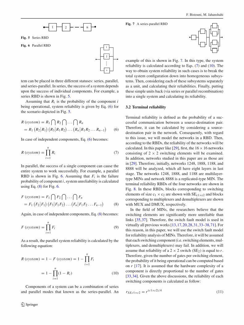
Fig. 5 Series RBD

Fig. 6 Parallel RBD

tem can be placed in three different statuses: series, parallel,and series-parallel. In series, the success of a system dependsupon the success of individual components. For example, aseries RBD is shown in Fig. 5.

Assuming that Ri is the probability of the component ibeing operational, system reliability is given by Eq. (6) forthe scenario depicted in Fig. 5.

R (system) = R1

⋂R2

⋂. . .

⋂Rn

= R1(R2

∣∣R1) (

R3∣∣R1R2

). . .

(Rn

∣∣R1R2 . . . Rn−1)

(6)

In case of independent components, Eq. (6) becomes:

R (system) =n∏

i=1

Ri (7)

In parallel, the success of a single component can cause theentire system to work successfully. For example, a parallelRBD is shown in Fig. 6. Assuming that Fi is the failureprobability of component i , system unreliability is calculatedusing Eq. (8) for Fig. 6.

F (system) = F1⋂

F2⋂

. . .⋂

Fn

= F1(F2

∣∣F1) (

F3∣∣F1F2

). . .

(Fn

∣∣F1F2 . . . Fn−1)

(8)

Again, in case of independent components, Eq. (8) becomes:

F (system) =n∏

i=1

Fi (9)

As a result, the parallel system reliability is calculated by thefollowing equation:

R (system) = 1 − F (system) = 1 −n∏

i=1

Fi

= 1 −n∏

i=1

(1 − Ri ) (10)

Components of a system can be a combination of seriesand parallel modes that known as the series-parallel. An

Fig. 7 A series-parallel RBD

example of this is shown in Fig. 7. In this type, the systemreliability is calculated according to Eqs. (7) and (10). Theway to obtain system reliability in such cases is to break thetotal system configuration down into homogeneous subsys-tems. Then, considering each of these subsystems separatelyas a unit, and calculating their reliabilities. Finally, puttingthese simple units back (via series or parallel recombination)into a single system and calculating its reliability.

3.2 Terminal reliability

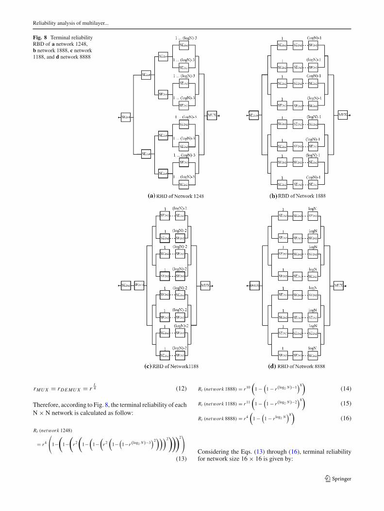
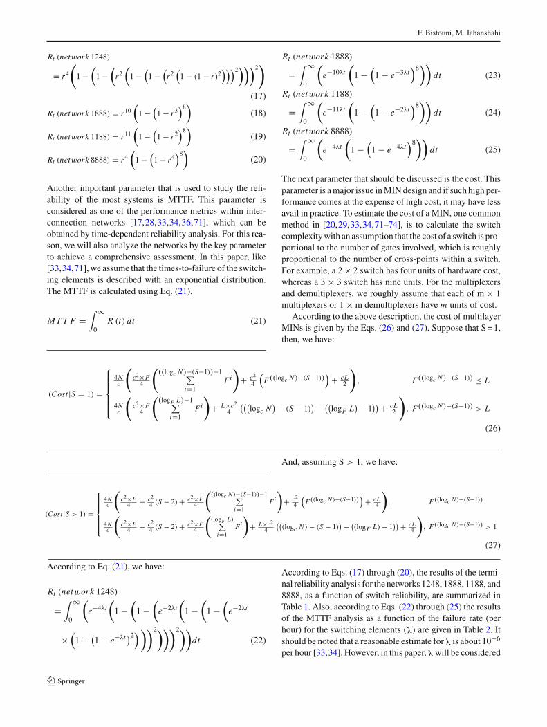
Terminal reliability is defined as the probability of a suc-cessful communication between a source-destination pair.Therefore, it can be calculated by considering a source-destination pair in the network. Consequently, with regardto this issue, we will model the networks in a RBD. Then,according to the RBDs, the reliability of the networks will becalculated. In this paper like [29], first, the 16×16 networksconsisting of 2 × 2 switching elements will be examined.In addition, networks studied in this paper are as those arein [29]. Therefore, initially, networks 1248, 1888, 1188, and8888 will be analyzed, which all have eight layers in laststage. The networks 1248, 1888, and 1188 are multilayer-type MINs and network 8888 is a replicated-type MIN. Theterminal reliability RBDs of the four networks are shown inFig. 8. In these RBDs, blocks corresponding to switchingelements of size c1 × c2 are shown with SEc1×c2 and blockscorresponding to multiplexers and demultiplexers are shownwith MUX and DMUX, respectively.

In the field of MINs, the researchers believe that theswitching elements are significantly more unreliable thanlinks [35,37]. Therefore, the switch fault model is used invirtually all previous works [13,17,20,28,31,33–38,71]. Forthis reason, in this paper, we will use the switch fault modelfor reliability analysis ofMINs. Therefore, it will be assumedthat each switching component (i.e. switching elements,mul-tiplexers, and demultiplexers) may fail. In addition, we willassume that reliability of a 2 × 2 switch (SE2) is equal to r .Therefore, given the number of gates per switching element,the probability of it being operational can be computed basedon r [17]. It is assumed that the hardware complexity of acomponent is directly proportional to the number of gates[33,34]. Given the above discussions, the reliability of eachswitching components is calculated as follow:

rSEc1×c2 = r (c1×c2)/4 (11)

123


Fig. 8 Terminal reliabilityRBD of a network 1248,b network 1888, c network1188, and d network 8888

rMUX = rDEMUX = rL4 (12)

Therefore, according to Fig. 8, the terminal reliability of eachN × N network is calculated as follow:

Rt (network 1248)

= r4

⎛

⎝1−(

1−(

r2(

1−(1−

(r2

(1−

(1−r(log2 N)−3

)2)))2)))2

⎞

⎠

(13)

Rt (network 1888) = r10(1 −

(1 − r(log2 N)−1

)8)(14)

Rt (network 1188) = r11(1 −

(1 − r(log2 N)−2

)8)(15)

Rt (network 8888) = r4(1 −

(1 − r log2 N

)8)(16)

Considering the Eqs. (13) through (16), terminal reliabilityfor network size 16 × 16 is given by:

123


Rt (network 1248)

= r4(

1 −(1 −

(r2

(1 −

(1 −

(r2

(1 − (1 − r)2

)))2)))2)

(17)

Rt (network 1888) = r10(1 −

(1 − r3

)8)(18)

Rt (network 1188) = r11(1 −

(1 − r2

)8)(19)

Rt (network 8888) = r4(1 −

(1 − r4

)8)(20)

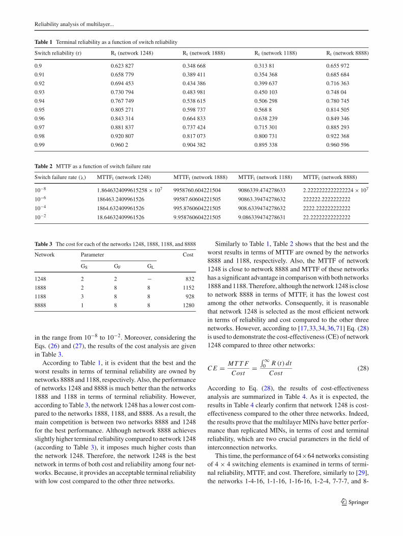
Another important parameter that is used to study the reli-ability of the most systems is MTTF. This parameter isconsidered as one of the performance metrics within inter-connection networks [17,28,33,34,36,71], which can beobtained by time-dependent reliability analysis. For this rea-son, we will also analyze the networks by the key parameterto achieve a comprehensive assessment. In this paper, like[33,34,71], we assume that the times-to-failure of the switch-ing elements is described with an exponential distribution.The MTTF is calculated using Eq. (21).

MTT F =∫ ∞

0R (t) dt (21)

According to Eq. (21), we have:

Rt (network 1248)

=∫ ∞

0

(e−4λt

(1 −

(1 −

(e−2λt

(1 −

(1 −

(e−2λt

×(1 − (

1 − e−λt)2)))2)))2))

dt (22)

Rt (network 1888)

=∫ ∞

0

(e−10λt

(1 −

(1 − e−3λt

)8))dt (23)

Rt (network 1188)

=∫ ∞

0

(e−11λt

(1 −

(1 − e−2λt

)8))dt (24)

Rt (network 8888)

=∫ ∞

0

(e−4λt

(1 −

(1 − e−4λt

)8))dt (25)

The next parameter that should be discussed is the cost. Thisparameter is amajor issue inMINdesign and if such high per-formance comes at the expense of high cost, it may have lessavail in practice. To estimate the cost of a MIN, one commonmethod in [20,29,33,34,71–74], is to calculate the switchcomplexitywith an assumption that the cost of a switch is pro-portional to the number of gates involved, which is roughlyproportional to the number of cross-points within a switch.For example, a 2× 2 switch has four units of hardware cost,whereas a 3 × 3 switch has nine units. For the multiplexersand demultiplexers, we roughly assume that each of m × 1multiplexers or 1 × m demultiplexers have m units of cost.

According to the above description, the cost of multilayerMINs is given by the Eqs. (26) and (27). Suppose that S=1,then, we have:

(Cost |S = 1) =

⎧⎪⎪⎪⎪⎨

⎪⎪⎪⎪⎩

4Nc

(c2×F4

(((logc N)−(S−1))−1∑

i=1Fi

)

+ c24

(F((logc N)−(S−1))

)+ cL

2

)

, F((logc N)−(S−1)) ≤ L

4Nc

(c2×F4

((logF L)−1∑

i=1Fi

)

+ L×c24

(((logc N

) − (S − 1)) − ((

logF L) − 1

)) + cL2

)

, F((logc N)−(S−1)) > L

(26)

And, assuming S > 1, we have:

(Cost |S > 1) =

⎧⎪⎪⎪⎪⎨

⎪⎪⎪⎪⎩

4Nc

(c2×F

4 + c24 (S − 2) + c2×F

4

(((logc N )−(S−1))−1∑

i=1Fi

)

+ c24

(F((logc N )−(S−1))

)+ cL

4

)

, F((logc N )−(S−1))

4Nc

(c2×F

4 + c24 (S − 2) + c2×F

4

((logF L)∑

i=1Fi

)

+ L×c24

(((logc N ) − (S − 1)

) − ((logF L) − 1

)) + cL4

)

, F((logc N )−(S−1)) > 1

(27)

According to Eqs. (17) through (20), the results of the termi-nal reliability analysis for the networks 1248, 1888, 1188, and8888, as a function of switch reliability, are summarized inTable 1. Also, according to Eqs. (22) through (25) the resultsof the MTTF analysis as a function of the failure rate (perhour) for the switching elements (λ) are given in Table 2. Itshould be noted that a reasonable estimate forλ is about 10−6

per hour [33,34]. However, in this paper,λwill be considered

123


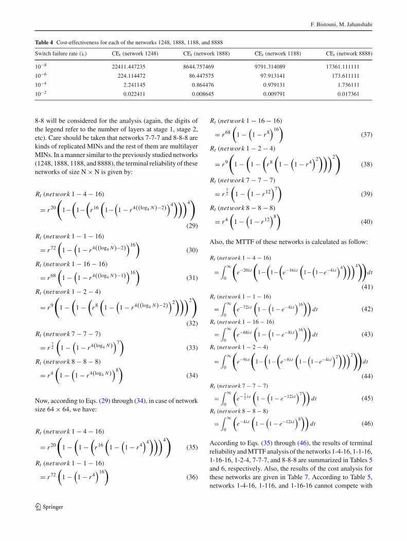
Table 1 Terminal reliability as a function of switch reliability

Switch reliability (r) Rt (network 1248) Rt (network 1888) Rt (network 1188) Rt (network 8888)

0.9 0.623 827 0.348 668 0.313 81 0.655 972

0.91 0.658 779 0.389 411 0.354 368 0.685 684

0.92 0.694 453 0.434 386 0.399 637 0.716 363

0.93 0.730 794 0.483 981 0.450 103 0.748 04

0.94 0.767 749 0.538 615 0.506 298 0.780 745

0.95 0.805 271 0.598 737 0.568 8 0.814 505

0.96 0.843 314 0.664 833 0.638 239 0.849 346

0.97 0.881 837 0.737 424 0.715 301 0.885 293

0.98 0.920 807 0.817 073 0.800 731 0.922 368

0.99 0.960 2 0.904 382 0.895 338 0.960 596

Table 2 MTTF as a function of switch failure rate

Switch failure rate (λ) MTTFt (network 1248) MTTFt (network 1888) MTTFt (network 1188) MTTFt (network 8888)

10−8 1.8646324099615258 × 107 9958760.604221504 9086339.474278633 2.2222222222222224 × 107

10−6 186463.2409961526 99587.60604221505 90863.39474278632 222222.2222222222

10−4 1864.632409961526 995.8760604221505 908.6339474278632 2222.222222222222

10−2 18.64632409961526 9.958760604221505 9.086339474278631 22.22222222222222

Table 3 The cost for each of the networks 1248, 1888, 1188, and 8888

Network Parameter Cost

GS GF GL

1248 2 2 − 832

1888 2 8 8 1152

1188 3 8 8 928

8888 1 8 8 1280

in the range from 10−8 to 10−2. Moreover, considering theEqs. (26) and (27), the results of the cost analysis are givenin Table 3.

According to Table 1, it is evident that the best and theworst results in terms of terminal reliability are owned bynetworks 8888 and 1188, respectively. Also, the performanceof networks 1248 and 8888 is much better than the networks1888 and 1188 in terms of terminal reliability. However,according to Table 3, the network 1248 has a lower cost com-pared to the networks 1888, 1188, and 8888. As a result, themain competition is between two networks 8888 and 1248for the best performance. Although network 8888 achievesslightly higher terminal reliability compared to network 1248(according to Table 3), it imposes much higher costs thanthe network 1248. Therefore, the network 1248 is the bestnetwork in terms of both cost and reliability among four net-works. Because, it provides an acceptable terminal reliabilitywith low cost compared to the other three networks.

Similarly to Table 1, Table 2 shows that the best and theworst results in terms of MTTF are owned by the networks8888 and 1188, respectively. Also, the MTTF of network1248 is close to network 8888 and MTTF of these networkshas a significant advantage in comparisonwith both networks1888 and1188.Therefore, although the network1248 is closeto network 8888 in terms of MTTF, it has the lowest costamong the other networks. Consequently, it is reasonablethat network 1248 is selected as the most efficient networkin terms of reliability and cost compared to the other threenetworks. However, according to [17,33,34,36,71] Eq. (28)is used to demonstrate the cost-effectiveness (CE) of network1248 compared to three other networks:

CE = MTT F

Cost=

∫ ∞0 R (t) dt

Cost(28)

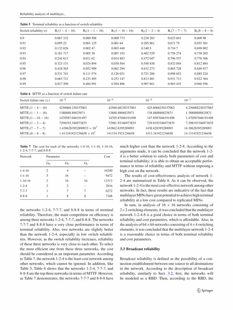
According to Eq. (28), the results of cost-effectivenessanalysis are summarized in Table 4. As it is expected, theresults in Table 4 clearly confirm that network 1248 is cost-effectiveness compared to the other three networks. Indeed,the results prove that the multilayer MINs have better perfor-mance than replicated MINs, in terms of cost and terminalreliability, which are two crucial parameters in the field ofinterconnection networks.

This time, the performance of 64×64 networks consistingof 4 × 4 switching elements is examined in terms of termi-nal reliability, MTTF, and cost. Therefore, similarly to [29],the networks 1-4-16, 1-1-16, 1-16-16, 1-2-4, 7-7-7, and 8-

123


Table 4 Cost-effectiveness for each of the networks 1248, 1888, 1188, and 8888

Switch failure rate (λ) CEt (network 1248) CEt (network 1888) CEt (network 1188) CEt (network 8888)

10−8 22411.447235 8644.757469 9791.314089 17361.111111

10−6 224.114472 86.447575 97.913141 173.611111

10−4 2.241145 0.864476 0.979131 1.736111

10−2 0.022411 0.008645 0.009791 0.017361

8-8 will be considered for the analysis (again, the digits ofthe legend refer to the number of layers at stage 1, stage 2,etc). Care should be taken that networks 7-7-7 and 8-8-8 arekinds of replicated MINs and the rest of them are multilayerMINs. In amanner similar to the previously studied networks(1248, 1888, 1188, and 8888), the terminal reliability of thesenetworks of size N × N is given by:

Rt (network 1 − 4 − 16)

= r20(

1−(1−

(r16

(1−

(1 − r4((log4 N)−2)

)4)))4)

(29)

Rt (network 1 − 1 − 16)

= r72(1 −

(1 − r4((log4 N)−2)

)16)(30)

Rt (network 1 − 16 − 16)

= r68(1 −

(1 − r4((log4 N)−1)

)16)(31)

Rt (network 1 − 2 − 4)

= r9(

1 −(1 −

(r8

(1 −

(1 − r4((log4 N)−2)

)2)))2)

(32)


= r72

(1 −

(1 − r4(log4 N)

)7)(33)


= r4(1 −

(1 − r4(log4 N)

)8)(34)

Now, according to Eqs. (29) through (34), in case of networksize 64 × 64, we have:

Rt (network 1 − 4 − 16)

= r20(

1 −(1 −

(r16

(1 −

(1 − r4

)4)))4)

(35)

Rt (network 1 − 1 − 16)

= r72(1 −

(1 − r4

)16)(36)

Rt (network 1 − 16 − 16)

= r68(1 −

(1 − r8

)16)(37)


= r9(

1 −(1 −

(r8

(1 −

(1 − r4

)2)))2)

(38)


= r72

(1 −

(1 − r12

)7)(39)


= r4(1 −

(1 − r12

)8)(40)

Also, the MTTF of these networks is calculated as follow:

Rt (network 1 − 4 − 16)

=∫ ∞

0

(

e−20λt

(

1−(1−

(e−16λt

(1−

(1−e−4λt

)4)))4))

dt

(41)Rt (network 1 − 1 − 16)

=∫ ∞

0

(e−72λt

(1 −

(1 − e−4λt

)16))dt (42)

Rt (network 1 − 16 − 16)

=∫ ∞

0

(e−68λt

(1 −

(1 − e−8λt

)16))dt (43)


=∫ ∞

0

(

e−9λt

(

1−(1−

(e−8λt

(1−

(1−e−4λt

)2)))2))

dt

(44)Rt (network 7 − 7 − 7)

=∫ ∞

0

(e− 7

2 λt(1 −

(1 − e−12λt

)7))dt (45)


=∫ ∞

0

(e−4λt

(1 −

(1 − e−12λt

)8))dt (46)

According to Eqs. (35) through (46), the results of terminalreliability andMTTFanalysis of the networks 1-4-16, 1-1-16,1-16-16, 1-2-4, 7-7-7, and 8-8-8 are summarized in Tables 5and 6, respectively. Also, the results of the cost analysis forthese networks are given in Table 7. According to Table 5,networks 1-4-16, 1-116, and 1-16-16 cannot compete with

123


Table 5 Terminal reliability as a function of switch reliability

Switch reliability (r) Rt(1 − 4 − 16) Rt(1 − 1 − 16) Rt(1 − 16 − 16) Rt(1 − 2 − 4) Rt(7 − 7 − 7) Rt(8 − 8 − 8)

0.9 0.067 332 0.000 508 0.000 773 0.238 283 0.623 841 0.609 98

0.91 0.095 22 0.001 125 0.001 64 0.285 861 0.671 75 0.655 301

0.92 0.132 626 0.002 47 0.003 448 0.340 5 0.716 7 0.698 082

0.93 0.181 717 0.005 38 0.007 192 0.402 529 0.758 274 0.738 285

0.94 0.244 613 0.011 62 0.014 883 0.472 047 0.796 537 0.776 306

0.95 0.323 131 0.024 894 0.030 564 0.548 838 0.832 044 0.812 884

0.96 0.418 565 0.052 909 0.062 294 0.632 273 0.865 728 0.848 917

0.97 0.531 741 0.111 574 0.126 031 0.721 206 0.898 652 0.885 224

0.98 0.663 721 0.233 495 0.253 147 0.813 881 0.931 713 0.922 364

0.99 0.817 509 0.484 991 0.504 886 0.907 861 0.965 435 0.960 596

Table 6 MTTF as a function of switch failure rate

Switch failure rate (λ) 10−8 10−6 10−4 10−2

MTTFt(1 − 4 − 16) 4256068.230337063 42560.68230337063 425.6068230337063 4.256068230337063

MTTFt(1 − 1 − 16) 1388888.88825871 13888.8888825871 138.888888825871 1.38888888825871

MTTFt(1 − 16 − 16) 1470587.046191497 14705.87046191498 147.0587046191498 1.470587046191498

MTTFt(1 − 2 − 4) 7298193.346973835 72981.93346973835 729.8193346973835 7.298193346973835

MTTFt(7 − 7 − 7) 1.4386283952890933 × 107 143862.8395289093 1438.628395289093 14.38628395289093

MTTFt(8 − 8 − 8) 1.413341921236658 × 107 141334.1921236658 1413.341921236658 14.13341921236658

Table 7 The cost for each of the networks 1-4-16, 1-1-16, 1-16-16,1-2-4, 7-7-7, and 8-8-8

Network Parameter Cost

GS GF GL

1-4-16 2 4 – 10240

1-1-16 3 16 – 9472

1-16-16 2 16 16 13312

1-2-4 2 2 – 2816

7-7-7 1 7 7 6272

8-8-8 1 8 8 7168

the networks 1-2-4, 7-7-7, and 8-8-8 in terms of terminalreliability. Therefore, the main competition on efficiency isamong three networks 1-2-4, 7-7-7, and 8-8-8. The networks7-7-7 and 8-8-8 have a very close performance in terms ofterminal reliability. Also, two networks are slightly betterthan the network 1-2-4, especially in low switch reliabili-ties. However, as the switch reliability increases, reliabilityof these three networks is very close to each other. To selectthe most efficient one from these three networks, the costshould be considered as an important parameter. Accordingto Table 7, the network 1-2-4 is the least-cost network amongother networks, which cannot be ignored. In addition, likeTable 5, Table 6 shows that the networks 1-2-4, 7-7-7, and8-8-8 are the top three networks in terms ofMTTF. However,as Table 7 demonstrates, the networks 7-7-7 and 8-8-8 have

much higher cost than the network 1-2-4. According to thearguments made, it can be concluded that the network 1-2-4 is a better solution to satisfy both parameters of cost andterminal reliability; it is able to obtain an acceptable perfor-mance in terms of reliability and MTTF without imposing ahigh cost on the network.

The results of cost-effectiveness analysis of network 1-2-4 are summarized in Table 8. As it can be observed, thenetwork 1-2-4 is themost cost-effective network amongothernetworks. In fact, these results are indicative of the fact thatmultilayerMINs have great potential to achieve high terminalreliability at a low cost compared to replicated MINs.

In sum, in analysis of 16 × 16 networks consisting of2×2 switching elements, it was concluded that themultilayernetwork 1-2-4-8 is a good choice in terms of both terminalreliability and cost parameters, which is affordable. Also, inthe analysis of 64×64 networks consisting of 4×4 switchingelements, it was concluded that the multilayer network 1-2-4is a reasonable choice in terms of both terminal reliabilityand cost parameters.

3.3 Broadcast reliability

Broadcast reliability is defined as the possibility of a con-nection establishment between one source to all destinationsin the network. According to the description of broadcastreliability, similarly to Sect. 3.2, first, the networks willbe modeled as a RBD. Then, according to the RBD, the

123


Table 8 Cost-effectiveness ofpoint-terminal for each of thenetworks 1-4-16, 1-1-16,1-16-16, 1-2-4, 7-7-7, and 8-8-8


CEt(1-4-16) 415.631663 4.156317 0.041563 0.000416

CEt(1-1-16) 146.631006 1.46631 0.014663 0.000147

CEt(1-16-16) 110.470782 1.104708 0.011047 0.00011

CEt(1-2-4) 2591.687978 25.91688 0.259169 0.002592

CEt(7-7-7) 2293.731498 22.937315 0.229373 0.002294

CEt(8-8-8) 2253.415053 22.534151 0.225342 0.002253

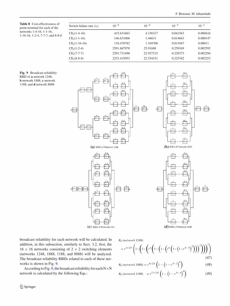
Fig. 9 Broadcast reliabilityRBD of a network 1248,b network 1888, c network1188, and d network 8888

broadcast reliability for each network will be calculated. Inaddition, in this subsection, similarly to Sect. 3.2, first, the16 × 16 networks consisting of 2 × 2 switching elements(networks 1248, 1888, 1188, and 8888) will be analyzed.The broadcast reliability RBDs related to each of these net-works is shown in Fig. 9.

According toFig. 9, the broadcast reliability for eachN×Nnetwork is calculated by the following Eqs.:

Rb (network 1248)

= r2+2N

⎛

⎝1−(

1−(

r4(

1−(1−

(r8

(1−

(1−r N−8

)2)))2)))2

⎞

⎠

(47)

Rb (network 1888) = r8+2N(1 −

(1 − r N−2

)8)(48)

Rb (network 1188) = r17+2N(1 −

(1 − r N−4

)8)(49)

123


Table 9 Broadcast reliability as a function of switch reliability

Switch reliability (r) Rb (network 1248) Rb (network 1888) Rb (network 1188) Rb (network 8888)

0.9 0.015183 0.012931 0.005324 0.023415

0.91 0.025203 0.021081 0.009404 0.036129

0.92 0.041036 0.033801 0.016382 0.054767

0.93 0.065479 0.053362 0.028181 0.081627

0.94 0.102315 0.083092 0.04795 0.119815

0.95 0.15852 0.127902 0.080833 0.173621

0.96 0.234514 0.195114 0.135229 0.249104

0.97 0.344587 0.29565 0.224792 0.354892

0.98 0.497724 0.445694 0.3716 0.503126

0.99 0.709051 0.668972 0.611117 0.710553

Table 10 MTTF of point-broadcast as a function of switch failure rate

Switch failure rate (λ) MTTFb (network 1248) MTTFb (network 1888) MTTFb (network 1188) MTTFb (network 8888)

10−8 2753202.762817228 2482012.9467939287 2037027.54425225 2896068.1174419126

10−6 27532.027640461245 24820.12946997553 20370.275451832702 28960.68117057186

10−4 275.320276485077 248.20129477386715 203.70275458758874 289.60681178778754

10−2 2.753202574996651 2.4820129499749735 2.0370275173078976 2.8960681536519672

Rb (network 8888) = r2+2N(1 −

(1 − r N−1

)8)(50)

As a result, for the size 16 × 16, we have:

Rb (network 1248)

= r34

⎛

⎝1−(

1−(

r4(

1−(1−

(r8

(1−

(1−r8

)2)))2)))2

⎞

⎠

(51)

Rb (network 1888) = r40(1 −

(1 − r14

)8)(52)

Rb (network 1188) = r49(1 −

(1 − r12

)8)(53)

Rb (network 8888) = r34(1 −

(1 − r15

)8)(54)

Also, the MTTF of point-broadcast is given by the followingEqs.:

Rb (network 1248)

=∫ ∞

0

(e−34λt

(1 −

(1 −

(e−4λt

(1 −

(1 − (e−8λt

×(1 −

(1 − e−8λt

)2)))2)))2))dt (55)

Rb (network 1888)

=∫ ∞

0

(e−40λt

(1 −

(1 − e−14λt

)8))dt (56)

Rb (network 1188)

=∫ ∞

0

(e−49λt

(1 −

(1 − e−12λt

)8))dt (57)

Rb (network 8888)

=∫ ∞

0

(e−34λt

(1 −

(1 − e−15λt

)8))dt (58)

According to the Eqs. (51) through (58), the results of thereliability and MTTF analyzes is given in Tables 9 and 10,respectively.According toTable 9, it is clear that the networks1888 and 1188 have less broadcast reliability compared to thenetworks 1248 and 8888. Although these results show thatthe network 8888 is slightly better than the network 1248 interms of broadcast reliability, both of them achieve a veryclose results. On the other hand, according to Table 3, itwas demonstrated that the network 1248 had been the least-cost network among four networks. Therefore, similarly toSect. 3.2, it is rational to choose the network 1248 as themost efficient network compared to the other three networksconsidering both reliability and cost parameters.

Table 10 also indicates the fact that the networks 1248and 8888 have the best performance in terms of MTTF.However, according to Table 3, the network 1248 is a betterchoice due to its cost-effectiveness. In order to fully prove thecost-effectiveness of network 1248 compared to three othernetworks, the results of cost-effectiveness of point-broadcastanalysis are summarized in Table 11. As Table 11 shows, thehighest value in terms of cost-effectiveness is owned by thenetwork 1248. Therefore, it can be concluded that the idea of

123


Table 11 Cost-effectiveness of point-broadcast for each of the networks 1248, 1888, 1188, and 8888

Switch failure rate (λ) CEb (network 1248) CEb (network 1888) CEb (network 1188) CEb (network 8888)

10−8 3309.137936 2154.525127 2195.072785 2262.553217

10−6 33.091379 21.545251 21.950728 22.625532

10−4 0.330914 0.215453 0.219507 0.226255

10−2 0.003309 0.002155 0.002195 0.002263

multilayer MINs can lead to cost-effective topologies, whichhave also high broad cast reliability.

In the next analysis, the performance of 64×64 networksconsisting of 4×4 switching elements, the networks 1-4-16,1-1-16, 1-16-16, 1-2-4, 7-7-7, and 8-8-8 will be examined.Similarly to the previous analysis, the broadcast reliability ofthese networks for size N×N is calculated by the followingEqs.:

Rb (network 1 − 4 − 16)

= r16+4N

⎛

⎝1 −(

1 −(

r64(

1−(1−r

4(N−163

))4)))4

⎞

⎠

(59)

Rb (network 1 − 1 − 16)

= r68+4N

(

1 −(1 − r

4(N−163

))16)

(60)

Rb (network 1 − 16 − 16)

= r64+4N

(

1 −(1 − r

4(N−43

))16)

(61)

Rb (network 1 − 2 − 4)

= r8+N

⎛

⎝1 −(

1 −(

r32(

1 −(1 − r

4(N−163

))2)))2

⎞

⎠

(62)


= r7N+7

4

(

1 −(1 − r

4(N−13

))7)

(63)


= r2+2N

(

1 −(1 − r

4(N−13

))8)

(64)

According to Eqs. (59) through (64), the broadcast reliabilityfor the networks of size 64× 64 is obtained by the followingequations:

Rb (network 1 − 4 − 16)

= r272(

1 −(1 −

(r64

(1 −

(1 − r64

)4)))4)

(65)

Rb (network 1 − 1 − 16)

= r324(1 −

(1 − r64

)16)(66)

Rb (network 1 − 16 − 16)

= r320(1 −

(1 − r80

)16)(67)


= r72(

1 −(1 −

(r32

(1 −

(1 − r64

)2)))2)

(68)


= r4554

(1 −

(1 − r84

)7)(69)


= r130(1 −

(1 − r84

)8)(70)

Moreover, the MTTF of point-broadcast for each network iscalculated as follow:

Rb (network 1 − 4 − 16)

=∫ ∞

0

(e−272λt

(1−

(1−

(e−64λt

(1−(

1−e−64λt )4)))4))

dt

(71)Rb (network 1 − 1 − 16)

=∫ ∞

0

(e−324λt

(1 − (

1 − e−64λt )16))

dt (72)

Rb (network 1 − 16 − 16)

=∫ ∞

0

(e−320λt

(1 − (

1 − e−80λt )16))

dt (73)


=∫ ∞

0

(e−72λt

(1−

(1−

(e−32λt

(1−(

1−e−64λt )2)))2))

dt

(74)Rb (network 7 − 7 − 7)

=∫ ∞

0

(e− 455

4 λt(1 − (

1 − e−84λt )7))

dt (75)


=∫ ∞

0

(e−130λt

(1 − (

1 − e−84λt )8))

dt (76)

The results of broadcast reliability and MTTF of point-broadcast analysis are shown in Tables 12 and 13, respec-tively. As the tables show, the networks 1-4-16, 1-1-16, and

123


1-16-16 because of poor results cannot compete with the net-works 1-2-4, 7-7-7, and 8-8-8 in terms of broadcast reliabilityand MTTF. On the other hand, the results demonstrate thatthe network 1-2-4 has the best performance compared to thenetworks 7-7-7 and 8-8-8 in terms of broadcast reliability andMTTF of point-broadcast. In addition, according to Table 7,it was proven that the network 1-2-4 had been the least-costamong six networks. Therefore, network 1-2-4 is the bestchoice for both the broadcast reliability and cost.

To complete thediscussion, the results of cost-effectivenessanalysis are shown in Table 14. Table 14 shows that net-work 1-2-4 is the most cost-effective network among othernetworks. These results reflect the fact that the multilayerMINs have a greater potential for providing two importantparameters of broadcast reliability and cost, compared to thereplicated MINs.

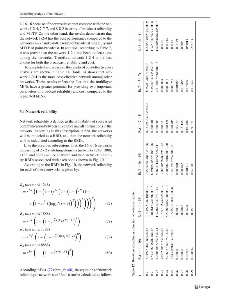
3.4 Network reliability

Network reliability is defined as the probability of successfulcommunicationbetween all sources and all destinations in thenetwork. According to this description, at first, the networkswill be modeled as a RBD, and then the network reliabilitywill be calculated according to the RBDs.

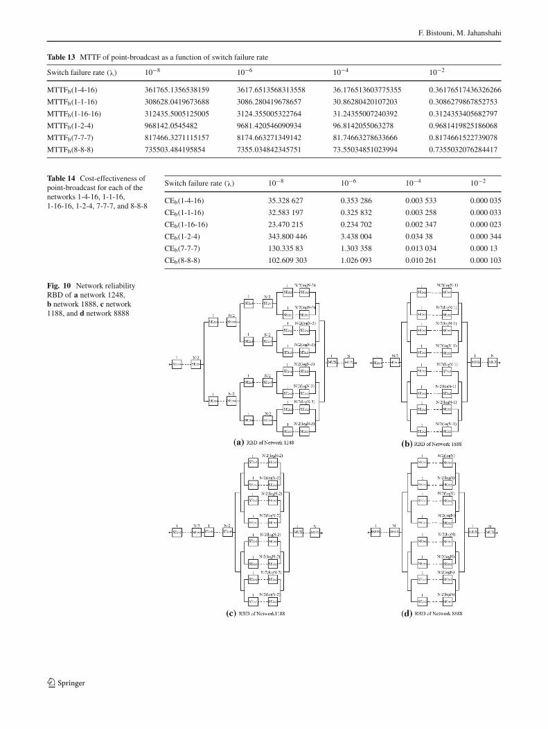
Like the previous subsections, first, the 16× 16 networksconsisting of 2×2 switching elements (networks 1248, 1888,1188, and 8888) will be analyzed and then, network reliabil-ity RBDs associated with each one is shown in Fig. 10.

According to the RBDs in Fig. 10, the network reliabilityfor each of these networks is given by:

Rn (network 1248)

= r3N(1 −

(1 −

(r N

(1 −

(1 −

(r N

(1−

×(1 − r

N2

((log2 N

) − 3))2

)))2)))2

⎞

⎠ (77)

Rn (network 1888)

= r6N(1 −

(1 − r

N2 ((log2 N)−1)

)8)(78)

Rn (network 1188)

= r13N2

(1 −

(1 − r

N2 ((log2 N)−2)

)8)(79)

Rn (network 8888)

= r4N(1 −

(1 − r

N2 (log2 N)

)8)(80)

According toEqs. (77) through (80), the equations of networkreliability to network size 16×16 can be calculated as follow: Ta

ble12

Broadcastrelia

bilityas

afunctio

nof

switc

hrelia

bility

rRb(1

−4

−16

)Rb(1

−1

−16

)Rb(1

−16

−16

)Rb(1

−2

−4)

Rb(7

−7

−7)

Rb(8

−8

−8)

0.9

7.94972316428074E-18

2.79497219821819E-17

7.95082663481238E-18

8.21349333703834E-8

6.2570198007455E

-91.29053305237407E-9

0.91

6.59331623870778E-16

2.01561737445077E-15

6.59105985523186E-16

0.000001

5.55982242745457E-8

1.37213476579393E-8

0.92

5.20061032235253E-14

1.3746414047872E

-13

5.1895114085152E

-14

0.000003

4.81900979661001E-7

1.42005404644458E-7

0.93

3.89757067153724E-12

8.79970157429262E-12

3.86830576980396E-12

0.00002

0.000004

0.000001

0.94

2.76632768287561E-10

5.20888504572868E-10

2.70608270184503E-10

0.000121

0.000033

0.000014

0.95

1.84320918103762E-8

2.77352110809128E-8

1.74019479557306E-8

0.000705

0.000265

0.00013

0.96

0.000001

0.000001

0.000001

0.003972

0.001983

0.001149

0.97

0.00006

0.000047

0.000045

0.021155

0.013485

0.00906

0.98

0.002411

0.001428

0.001512

0.101488

0.076094

0.058013

0.99

0.060884

0.03853

0.040108

0.391871

0.312549

0.267733

123


Table 13 MTTF of point-broadcast as a function of switch failure rate


MTTFb(1-4-16) 361765.1356538159 3617.6513568313558 36.176513603775355 0.36176517436326266

MTTFb(1-1-16) 308628.0419673688 3086.280419678657 30.86280420107203 0.3086279867852753

MTTFb(1-16-16) 312435.5005125005 3124.355005322764 31.24355007240392 0.3124353405682797

MTTFb(1-2-4) 968142.0545482 9681.420546090934 96.8142055063278 0.9681419825186068

MTTFb(7-7-7) 817466.3271115157 8174.663271349142 81.74663278633666 0.8174661522739078

MTTFb(8-8-8) 735503.484195854 7355.034842345751 73.55034851023994 0.7355032076284417

Table 14 Cost-effectiveness ofpoint-broadcast for each of thenetworks 1-4-16, 1-1-16,1-16-16, 1-2-4, 7-7-7, and 8-8-8


CEb(1-4-16) 35.328 627 0.353 286 0.003 533 0.000 035

CEb(1-1-16) 32.583 197 0.325 832 0.003 258 0.000 033

CEb(1-16-16) 23.470 215 0.234 702 0.002 347 0.000 023

CEb(1-2-4) 343.800 446 3.438 004 0.034 38 0.000 344

CEb(7-7-7) 130.335 83 1.303 358 0.013 034 0.000 13

CEb(8-8-8) 102.609 303 1.026 093 0.010 261 0.000 103

Fig. 10 Network reliabilityRBD of a network 1248,b network 1888, c network1188, and d network 8888

123


Table 15 Network reliability as a function of switch reliability

Switch reliability (r) Rn (network 1248) Rn (network 1888) Rn (network 1188) Rn (network 8888)

0.9 0.000 541 0.000 02 0.000 014 0.000 288

0.91 0.001 355 0.000 068 0.000 048 0.000 79

0.92 0.003 315 0.000 229 0.000 157 0.002 105

0.93 0.007 896 0.000 741 0.000 501 0.005 403

0.94 0.018 238 0.002 295 0.001 565 0.013 255

0.95 0.040 629 0.006 81 0.004 776 0.030 822

0.96 0.086 705 0.019 403 0.014 289 0.067 481

0.97 0.175 828 0.053 433 0.042 077 0.139 143

0.98 0.335 852 0.143 713 0.122 32 0.273 729

0.99 0.599 735 0.381 045 0.351 609 0.525 579

Table 16 MTTF of point-network as a function of switch failure rate

Switch failure rate (λ) MTTFn (network 1248) MTTFn (network 1888) MTTFn (network 1188) MTTFn (network 8888)

10−8 1757724.670750557 1039562.2892624302 961321.798678224 1527777.777776152

10−6 17577.24670733699 10395.622895841287 9613.21798702277 15277.777777983547

10−4 175.77246714080468 103.95622902062402 96.13217992615348 152.7777778594781

10−2 1.7577246549291525 1.0395623416674948 0.9613216801096037 1.5277777086322266

Table 17 Cost-effectiveness of point-network for each of the networks 1248, 1888, 1188, and 8888

Switch failure rate (λ) CEn (network 1248) CEn (network 1888) CEn (network 1188) CEn (network 8888)

10−8 2 112.649 845 902.397 821 1 035.907 111 1 193.576 389

10−6 21.126 498 9.023 978 10.359 071 11.935 764

10−4 0.211 265 0.090 24 0.103 591 0.119 358

10−2 0.002 113 0.000 902 0.001 036 0.001 194

Rn (network 1248)

= r48(

1−(1−

(r16

(1−

(1−

(r16

(1−(

1−r8)2)))2)))2

)

(81)Rn (network 1888)

= r96(1 − (

1 − r24)8) (82)

Rn (network 1188)

= r104(1 − (

1 − r16)8) (83)

Rn (network 8888)

= r64(1 − (

1 − r32)8) (84)

Also, the MTTF of point-network is given by the followingequations:Rn (network 1248)

=∫ ∞

0

(e−48λt

(1 −

(1 −

(e−16λt (1 − (1−

×(e−16λt

(1−

(1−e−8λt

)2)))2)))2

⎞

⎠

⎞

⎠ dt (85)

Rn (network 1888)

=∫ ∞

0

(e−96λt

(1 −

(1 − e−24λt

)8))dt (86)

Rn (network 1188)

=∫ ∞

0

(e−104λt

(1 −

(1 − e−16λt

)8))dt (87)

Rn (network 8888)

=∫ ∞

0

(e−64λt

(1 −

(1 − e−32λt

)8))dt (88)

According to Eqs. (81) through (88), the results of networkreliability and MTTF analysis are summarized in Tables 15and 16, respectively. As Table 15 shows, the highest and low-est network reliability is owned by the networks 1248 and1188, respectively. On the other hand, Table 16 also showsthat network 1248 has the best performance among the othernetworks in terms of MTTF of point-network. In addition,according to Table 3, it was demonstrated that the network1248 is the least-cost network compared to the other threenetworks. Consequently, it is reasonable to choose network

123


1248 as the best network among four networks in terms ofcost and network reliability. Moreover, the results of cost-effectiveness analysis in Table 17, confirm that the network1248 is the most affordable network compared to the otherthree networks. Therefore, it can be concluded that the mul-tilayer MINs have a higher efficiency in comparison withthe replicated MINs in terms of reliability, cost, and cost-effectiveness.

Here, the performance of 64 × 64 networks consisting of4×4 switching elements (the networks 1-4-16, 1-1-16, 1-16-16, 1-2-4, 7-7-7, and 8-8-8)will be examined. Similarly to theprevious analysis, the network reliability of these networksof size N × N is calculated by the following equations:

Rn (network 1 − 4 − 16)

= r8N(

1−(1−

(r4N

(1−

(1−r N((log4 N)−2)

)4)))4)

(89)

Rn (network 1 − 1 − 16)

= r21N(1 −

(1 − r N((log4 N)−2)

)16)(90)

Rn (network 1 − 16 − 16)

= r20N(1 −

(1 − r N((log4 N)−1)

)16)(91)

Rn (network 1 − 2 − 4)

= r3N(

1−(1−

(r2N

(1−

(1−r N((log4 N)−2)

)2)))2)

(92)


= r7N2

(1 −

(1 − r N(log4 N)

)7)(93)


= r4N(1 −

(1 − r N(log4 N)

)8)(94)

Therefore, considering the Eqs. (89) through (94), reliabilityequations for size 64 × 64 are given by:

Rn (network 1 − 4 − 16)

= r512(

1 −(1 −

(r256

(1 −

(1 − r64

)4)))4)

(95)

Rn (network 1 − 1 − 16)

= r1344(1 −

(1 − r64

)16)(96)

Rn (network 1 − 16 − 16)

= r1280(1 −

(1 − r128

)16)(97) Ta

ble18

Networkrelia

bilityas

afunctio

nof

switc

hrelia

bility

RRn(1-4-16)

Rn(1-1-16)

Rn(1-16-16)

Rn(1-2-4)

Rn(7-7-7)

Rn(8-8-8)

0.9

1.34421108731531E-37

5.93932540845249E-64

5.99195779222718E-64

1.07381009322923E-17

6.4562729739825E

-19

2.53357714859519E-20

0.91

1.33477314790267E-33

3.36223651787142E-57

3.42280173775187E-57

7.47196858374132E-16

6.40202273809694E-17

3.57794542444517E-18

0.92

1.1815386913263E

-29

1.59137786628338E-50

1.64932192369777E-50

4.96065750380977E-14

6.0371792581161E

-15

4.78670286118193E-16

0.93

9.45508649324501E-26

6.26722763368008E-44

6.72683081880809E-44

3.14354109680796E-12

5.42005234453769E-13

6.07364757845657E-14

0.94

6.82427693563417E-22

2.02840860768679E-37

2.32784805567728E-37

1.90105002401822E-10

4.63741660094131E-11

7.31741810087039E-12

0.95

4.42222804563885E-18

5.26149146311902E-31

6.82929401508471E-31

1.09566107630846E-8

3.78485286649694E-9

8.37885827743867E-10

0.96

2.54526506119947E-14

1.0479891596599E

-24

1.6771884378234E

-24

0.000001

2.94725013041205E-7

9.12016624282917E-8

0.97

1.27179528668147E-10

1.52163234210995E-18

3.26560547201867E-18

0.000031

0.000022

0.000009

0.98

0.000001

1.60426844462569E-12

4.20039881125473E-12

0.001449

0.001473

0.000873

0.99

0.001513

0.000001

0.000003

0.055513

0.070162

0.054561

123


Table 19 MTTF of point-network as a function of switch failure rate


MTTFn (1-4-16) 182171.3259755653 1821.713259755653 81.21713259755654 0.1821713259755653

MTTFn (1-1-16) 74404.76189898324 744.0476189898325 7.440476189898324 0.07440476189898323

MTTFn (1-16-16) 78124.98529199969 781.2498529799969 7.81249852919997 0.0781249852919997

MTTFn (1-2-4) 383748.1962481962 3837.481962481962 38.37481962481962 0.3837481962481962

MTTFn (7-7-7) 404222.3614398143 4042.223614398143 40.42223614398143 0.4042223614398143

MTTFn (8-8-8) 366369.2393133183 3663.692393133183 36.63692393133183 0.3663692393133183


= r192(

1 −(1 −

(r128

(1 −

(1 − r64

)2)))2)

(98)


= r224(1 −

(1 − r192

)7)(99)


= r256(1 −

(1 − r192

)8)(100)

Also, the MTTF of point-network for these networks is cal-culated as follow:

Rn (network 1 − 4 − 16)

=∫ ∞

0

(e−512λt

(1−

(1−

(e−256λt

(1−(

1−e−64λt )4)))4))

dt

(101)Rn (network 1 − 1 − 16)

=∫ ∞

0

(e−1344λt

(1 − (

1 − e−64λt )16))

dt (102)

Rn (network 1 − 16 − 16)

=∫ ∞

0

(e−1280λt

(1 − (

1 − e−128λt )16))

dt (103)


=∫ ∞

0

(e−192λt

(1−

(1−

(e−128λt

(1−(

1−e−64λt )2)))2))

dt

(104)Rn (network 7 − 7 − 7)

=∫ ∞

0

(e−224λt

(1 − (

1 − e−192λt )7))

dt (105)


=∫ ∞

0

(e−256λt

(1 − (

1 − e−192λt )8))

dt (106)

The results of network reliability and MTTF analysis for thenetworks 1-4-16, 1-1-16, 1-16-16, 1-2-4, 7-7-7, and 8-8-8are shown in Table 18 and 19, respectively.

According to Tables 18 and 19, it is clear that the net-works 1-4-16, 1-1-16, and 1-16-16 are not able to competewith the networks 1-2-4, 7-7-7, and 8-8-8 in terms of net-

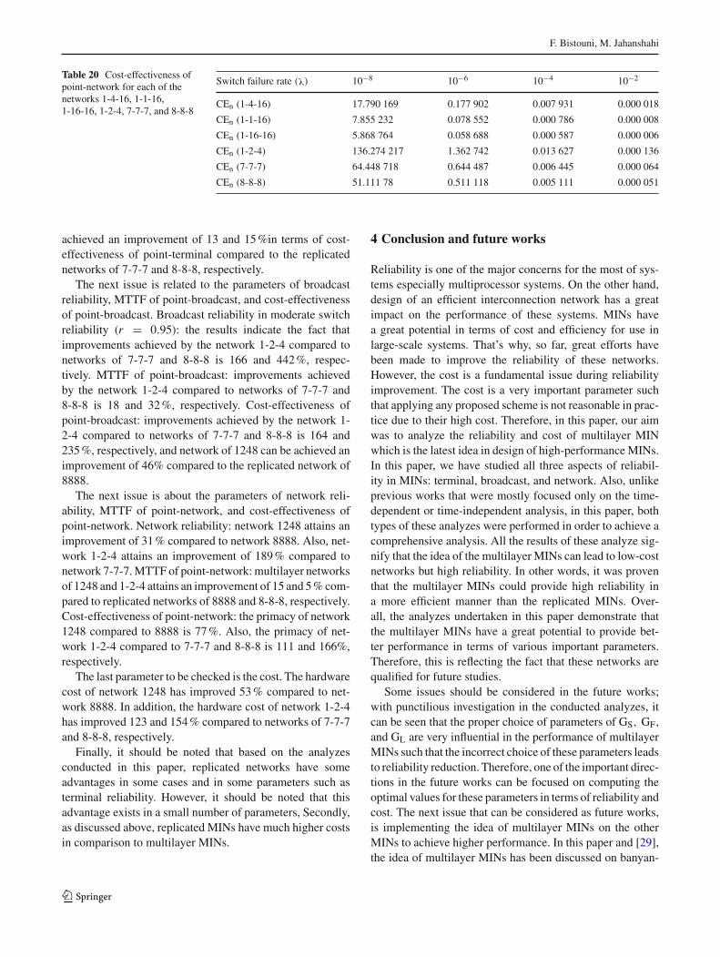
work reliability and MTTF. Therefore, the main competitionis among three networks 1-2-4, 7-7-7, and 8-8-8. As Tables18 and 19 shows, the three networks have a very close per-formance in terms of network reliability and MTTF. In thesecircumstances, which network is a more appropriate choice?To answer this question, the cost as another important para-meter should be considered. Considering Table 7, it is clearthat the network 1-2-4 has the least-cost in comparison withother five networks. Consequently, not only the network 1-2-4 provides an adequate reliability, but also is the least-costnetwork compared to other networks. Therefore, it is a moresensible choice compared to the other networks. To betterunderstand this issue, the results of cost-effectiveness analy-sis are given in Table 20. These results prove that the network1-2-4 is the most cost-effective network compared to the net-works 1-4-16, 1-1-16, 1-16-16, 7-7-7, and 8-8-8.

In sum, it can be concluded from the analyzes carriedout in Sect. 3 that the multilayer MIN 1248 of size 16 × 16and the multilayer MIN 1-2-4 of size 64× 64 achieve betterreliability and cost from different aspects of the terminal,broadcast, and network compared to other networks studiedin this paper. This means that although these networks have ahigh reliability, they do not impose high cost on the networkwhich makes them affordable. Indeed, the results of theseanalyzes are indicative of the fact that multilayer MINs havea higher potential to meet reliability requirements comparedto replicated MINs. For a more detailed discussion in thiscase, the percentage of improvement in various parametersfor these networks is analyzed in the next sub-section.

3.5 Discussion

In this sub-section, for a more detailed analysis, the per-centage of improvement in various parameters in multilayerMINs compared to replicated MINs will be quantified. Thefirst issue is about cost-effectiveness of point-terminal. Theresults of the analyses show that the multilayer network of1248 can be achieved an improvement of 29% in terms ofcost-effectiveness of point-terminal compared to the repli-cated network of 8888. Also, multilayer network of 1-2-4

123


Table 20 Cost-effectiveness ofpoint-network for each of thenetworks 1-4-16, 1-1-16,1-16-16, 1-2-4, 7-7-7, and 8-8-8


CEn (1-4-16) 17.790 169 0.177 902 0.007 931 0.000 018

CEn (1-1-16) 7.855 232 0.078 552 0.000 786 0.000 008

CEn (1-16-16) 5.868 764 0.058 688 0.000 587 0.000 006

CEn (1-2-4) 136.274 217 1.362 742 0.013 627 0.000 136

CEn (7-7-7) 64.448 718 0.644 487 0.006 445 0.000 064

CEn (8-8-8) 51.111 78 0.511 118 0.005 111 0.000 051

achieved an improvement of 13 and 15%in terms of cost-effectiveness of point-terminal compared to the replicatednetworks of 7-7-7 and 8-8-8, respectively.

The next issue is related to the parameters of broadcastreliability, MTTF of point-broadcast, and cost-effectivenessof point-broadcast. Broadcast reliability in moderate switchreliability (r = 0.95): the results indicate the fact thatimprovements achieved by the network 1-2-4 compared tonetworks of 7-7-7 and 8-8-8 is 166 and 442%, respec-tively. MTTF of point-broadcast: improvements achievedby the network 1-2-4 compared to networks of 7-7-7 and8-8-8 is 18 and 32%, respectively. Cost-effectiveness ofpoint-broadcast: improvements achieved by the network 1-2-4 compared to networks of 7-7-7 and 8-8-8 is 164 and235%, respectively, and network of 1248 can be achieved animprovement of 46% compared to the replicated network of8888.

The next issue is about the parameters of network reli-ability, MTTF of point-network, and cost-effectiveness ofpoint-network. Network reliability: network 1248 attains animprovement of 31% compared to network 8888. Also, net-work 1-2-4 attains an improvement of 189% compared tonetwork 7-7-7.MTTF of point-network:multilayer networksof 1248 and 1-2-4 attains an improvement of 15 and 5%com-pared to replicated networks of 8888 and 8-8-8, respectively.Cost-effectiveness of point-network: the primacy of network1248 compared to 8888 is 77%. Also, the primacy of net-work 1-2-4 compared to 7-7-7 and 8-8-8 is 111 and 166%,respectively.

The last parameter to be checked is the cost. The hardwarecost of network 1248 has improved 53% compared to net-work 8888. In addition, the hardware cost of network 1-2-4has improved 123 and 154% compared to networks of 7-7-7and 8-8-8, respectively.

Finally, it should be noted that based on the analyzesconducted in this paper, replicated networks have someadvantages in some cases and in some parameters such asterminal reliability. However, it should be noted that thisadvantage exists in a small number of parameters, Secondly,as discussed above, replicated MINs have much higher costsin comparison to multilayer MINs.

4 Conclusion and future works

Reliability is one of the major concerns for the most of sys-tems especially multiprocessor systems. On the other hand,design of an efficient interconnection network has a greatimpact on the performance of these systems. MINs havea great potential in terms of cost and efficiency for use inlarge-scale systems. That’s why, so far, great efforts havebeen made to improve the reliability of these networks.However, the cost is a fundamental issue during reliabilityimprovement. The cost is a very important parameter suchthat applying any proposed scheme is not reasonable in prac-tice due to their high cost. Therefore, in this paper, our aimwas to analyze the reliability and cost of multilayer MINwhich is the latest idea in design of high-performance MINs.In this paper, we have studied all three aspects of reliabil-ity in MINs: terminal, broadcast, and network. Also, unlikeprevious works that were mostly focused only on the time-dependent or time-independent analysis, in this paper, bothtypes of these analyzes were performed in order to achieve acomprehensive analysis. All the results of these analyze sig-nify that the idea of the multilayer MINs can lead to low-costnetworks but high reliability. In other words, it was proventhat the multilayer MINs could provide high reliability ina more efficient manner than the replicated MINs. Over-all, the analyzes undertaken in this paper demonstrate thatthe multilayer MINs have a great potential to provide bet-ter performance in terms of various important parameters.Therefore, this is reflecting the fact that these networks arequalified for future studies.

Some issues should be considered in the future works;with punctilious investigation in the conducted analyzes, itcan be seen that the proper choice of parameters of GS, GF,and GL are very influential in the performance of multilayerMINs such that the incorrect choice of these parameters leadsto reliability reduction. Therefore, one of the important direc-tions in the future works can be focused on computing theoptimal values for these parameters in terms of reliability andcost. The next issue that can be considered as future works,is implementing the idea of multilayer MINs on the otherMINs to achieve higher performance. In this paper and [29],the idea of multilayer MINs has been discussed on banyan-

123


like (typical)MINs. However, there aremany other advancedMINs that can be evaluated with the idea ofmultilayerMINs.

References

1. El-Rewini, H., & Abd-El-Barr, M. (2005). Advanced computerarchitecture and parallel processing. Hoboken: Wiley.

2. Duato, J., Yalamanchili, S., & Ni, L. M. (2003). Interconnectionnetworks: An engineering approach. Burlington: Morgan Kauf-mann.

3. Chan, K. S., et al. (2000). A refinedmodel for performance analysisof output-buffered Banyan networks. Telecommunication Systems,13.2–4, 393–411.

4. Pattavina, A., & Catania, C. (2003). Performance analysis of ATMreplicated banyan networks with external input-output queueing.Telecommunication Systems, 23(1–2), 149–170.

5. Gu, H., et al. (2010). A new distributed congestion control mecha-nism for networks on chip. Telecommunication Systems, 44(3–4),321–331.

6. Suboh, S., et al. (2008). An interconnection architecture fornetwork-on-chip systems. Telecommunication Systems, 37(1–3),137–144.

7. Agrawal, D. P., Chen, C., & Burke, J. R. (1998). Hybrid graph-based networks for multiprocessing. Telecommunication Systems,10(1–2), 107–134.

8. Bellaachia, A., & Youssef, A. (2000). Communication capabilitiesof product networks. Telecommunication Systems, 13(1), 119–133.

9. Jahanshahi, M., & Bistouni, F. (2015). Improving the reliability ofthe Benes network for use in large-scale systems.MicroelectronicsReliability, 55(3), 679–695.

10. Diab, H., Tabbara, H., & Mansour, N. (2000). Simulation ofdynamic input buffer space inmultistage interconnection networks.Advances in Engineering Software, 31(1), 13–24.

11. Jahanshahi, M., & Bistouni, F. (2014). A new approach to improvereliability of the multistage interconnection networks. Computers& Electrical Engineering, 40(8), 348–374.

12. Veglis, A., & Pomportsis, A. (2001). Dependability evaluation ofinterconnection networks. Computers & Electrical Engineering,27(3), 239–263.

13. Bistouni, F., & Jahanshahi, M. (2015). Scalable crossbar network:A non-blocking interconnection network for large-scale systems.Journal of Supercomputing, 71(2), 697–728.

14. Kolias, C., & Tomkos, I. (2005). Switch fabrics. IEEE Circuits andDevices Magazine, 21(5), 12–17.

15. Bataineh, S. M., & Allosl, B. Y. (2001). Fault-tolerant multistageinterconnection network. Telecommunication Systems, 17(4), 455–472.

16. Ayyaz, M. N., Meliksetian, D. S., & Roger Chen, C. Y. (2000).Partitionable multistage interconnection networks. Part 2: Taskmigration schemes. Telecommunication Systems, 13(1), 45–67.

17. Blake, J. T., & Trivedi, K. S. (1989). Reliability analysis ofinterconnection networks using hierarchical composition. IEEETransactions on Reliability, 38(1), 111–120.

18. Garofalakis, J., & Stergiou, E. (2010). Analytical model forperformance evaluation of multilayer multistage interconnectionnetworks servicing unicast and multicast traffic by partial multi-cast operation. Performance Evaluation, 67(10), 959–976.

19. Vasiliadis, D. C., Rizos, G. E., & Vassilakis, C. (2013). Modellingand performance study of finite-buffered blockingmultistage inter-connection networks supporting natively 2-class priority routingtraffic. Journal ofNetwork andComputerApplications,36(2), 723–737.

20. Bistouni, F., & Jahanshahi, M. (2014). Improved extra group net-work: A new fault-tolerant multistage interconnection network.Journal of Supercomputing, 69(1), 161–199.

21. Mahgoub, I., & Huang, C. J. (1998). A novel scheme to improvefault-tolerant capabilities of multistage interconnection networks.Telecommunication Systems, 10(1–2), 45–66.

22. Stergiou, E., & Garofalakis, J. (2012). Performance estimation ofbanyan semi layer networkswith drop resolutionmechanism. Jour-nal of Network and Computer Applications, 35(1), 287–294.

23. Garhwal, S., & Srivastava, N. (2011). Designing a fault-tolerantfully-chained combining switches multi-stage interconnection net-work with disjoint paths. Journal of Supercomputing, 55.3, 400–431.

24. Rajkumar, S., & Goyal, N. K. (2014). Design of 4-disjoint gammainterconnection network layouts and reliability analysis of gammainterconnection networks. Journal of Supercomputing, 69(1), 468–491.

25. Ferreira, R. S., et al. (2011). Fast placement and routing by extend-ing coarse-grained reconfigurable arrays with Omega Networks.Journal of Systems Architecture, 57(8), 761–777.

26. Zhang, Y.-H., et al. (2014). A method of batching conflict routingsin shuffle-exchange networks. Theoretical Computer Science, 522,24–33.

27. Jaros, J (2009). Evolutionary optimization of multistage intercon-nection networks performance. In Proceedings of the GECCOVol.9.

28. Blake, J.T., & Trivedi, K.S. (1988). Reliability of the shuffle-exchange network and its variants. In Proceedings of the twenty-first annual hawaii international conference on system sciences,Architecture Track (Vol. 1). IEEE.

29. Tutsch, D., &Hommel, G. (2008).MLMIN: Amulticore processorand parallel computer network topology for multicast. Computers& Operations Research, 35(12), 3807–3821.

30. Garofalakis, J., & Stergiou, E. (2011). Mechanisms and analy-sis for supporting multicast traffic by using multilayer multistageinterconnection networks. International Journal of Network Man-agement, 21(2), 130–146.

31. Bistouni, F., & Jahanshahi, M. (2014). Analyzing the reliability ofshuffle-exchange networks using reliability block diagrams. Reli-ability Engineering & System Safety, 132, 97–106.

32. Barranco, M., Proenza, J., & Almeida, L. (2015). Quantitativecharacterization of the reliability of simplex buses and stars to com-pare their benefits in fieldbuses. Reliability Engineering & SystemSafety, 138, 163–175. doi:10.1016/j.ress.2015.01.005.

33. Bistouni, F., & Jahanshahi, M. (2015). Pars network: A multistageinterconnection network with fault-tolerance capability. Journal ofParallel and Distributed Computing, 75, 168–183.

34. Bansal, P. K., Joshi, R. C., & Singh, K. (1994). On a fault-tolerantmultistage interconnection network. Computers & electrical engi-neering, 20(4), 335–345.

35. Rai, S., & Oh, Y. C. (1999). Tighter bounds on full access proba-bility in fault-tolerant multistage interconnection networks. IEEETransactions on Parallel and Distributed Systems, 10(3), 328–335.

36. Blake, J. T., & Trivedi, K. S. (1989). Multistage interconnec-tion network reliability. IEEE Transactions on Computers, 38(11),1600–1604.

37. Gunawan, I. (2008). Redundant paths and reliability bounds ingamma networks. Applied Mathematical Modelling, 32(4), 588–594.

38. Cheng, X., & Ibe, O. C. (1992). Reliability of a class of multistageinterconnection networks. IEEE Transactions on Parallel and Dis-tributed Systems, 3(2), 241–246.

39. Bauer, E. (2010).Design for reliability: Information and computer-based systems. Hoboken: Wiley.

40. Kang, W.-H., & Kliese, A. (2014). A rapid reliability estima-tion method for directed acyclic lifeline networks with statistically

123

http://dx.doi.org/10.1016/j.ress.2015.01.005


dependent components. Reliability Engineering & System Safety,124, 81–91.

41. Hong, L., et al. (2015). Vulnerability assessment andmitigation forthe Chinese railway system under floods. Reliability Engineering& System Safety, 137, 58–68.

42. Padmavathy, N., & Chaturvedi, S. K. (2013). Evaluation of mobilead hoc network reliability using propagation-based link reliabilitymodel. Reliability Engineering & System Safety, 115, 1–9.

43. Shuang, Q., Zhang, M., & Yuan, Y. (2014). Node vulnerability ofwater distribution networks under cascading failures. ReliabilityEngineering & System Safety, 124, 132–141.

44. Lee, A., & Ra, I. (2015). Network resource efficient routing inmobile ad hoc wireless networks. Telecommunication Systems,60(2), 215–223.

45. Nayebi, A., & Sarbazi-Azad, H. (2013). Optimum hello intervalfor a connected homogeneous topology in mobile wireless sensornetworks. Telecommunication Systems, 52(4), 2475–2488.

46. Jahanshahi, M., Dehghan, M., & Meybodi, M. R. (2013). LAMR:Learning automata based multicast routing protocol for multi-channel multi-radio wireless mesh networks. Applied Intelligence,38(1), 58–77.

47. Jahanshahi, M., Dehghan, M., &Meybodi, M. R. (2013). On chan-nel assignment and multicast routing in multi-channel multi-radiowireless mesh networks. International Journal of Ad Hoc andUbiquitous Computing, 12(4), 225–244.

48. Rak, J. (2015). A new approach to design of weather disruption-tolerant wireless mesh networks. Telecommunication Systems.doi:10.1007/s11235-015-0003-z.

49. Jahanshahi, M., Dehghan, M., & Meybodi, M. R. (2011). A math-ematical formulation for joint channel assignment and multicastrouting inmulti-channelmulti-radiowirelessmesh networks. Jour-nal of Network and Computer Applications, 34(6), 1869–1882.

50. Jahanshahi, M., & Barmi, A. T. (2014). Multicast routing protocolsin wireless mesh networks: A survey. Computing, 96(11), 1029–1057.

51. Jahanshahi, M., Maddah, M., & Najafizadegan, N. (2013). Energyaware distributed partitioning detection and connectivity restora-tion algorithm in wireless sensor networks. International Journalof Mathematical Modelling & Computations, 3.1, 71–82.

52. Liu, X., Zhang, S., & Bu, K. (2015). A locality-based range-freelocalization algorithm for anisotropic wireless sensor networks.Telecommunication Systems. doi:10.1007/s11235-015-9978-8.

53. Guerroumi,M., Badache, N., &Moussaoui, S. (2015). Mobile sinkand power management for efficient data dissemination in wirelesssensor networks. Telecommunication Systems, 58(4), 279–292.

54. Jahanshahi, M., Rahmani, S., & Ghaderi, S. (2013). An efficientcluster head selection algorithm for wireless sensor networks usingfuzzy inference systems. The International Journal of Smart Elec-trical Engineering (IJSEE), 2.2, 121–125.

55. Ebrahimi, N., McCullough, K., & Xiao, Z. (2013). Reliability ofsensors based on nanowire networks operating in a dynamic envi-ronment. IEEE Transactions on Reliability, 62(4), 908–916.

56. Schneider, K., et al. (2013). Social network analysis via multi-statereliability and conditional influence models. Reliability Engineer-ing & System Safety, 109, 99–109.

57. Lin, Y.-K., & Chang, P.-C. (2013). A novel reliability evaluationtechnique for stochastic-flow manufacturing networks with mul-tiple production lines. IEEE Transactions on Reliability, 62(1),92–104.

58. Chang, N.-W., et al. (2015). Conditional diagnosability of (n,k)-star networks under the comparison diagnosis model. IEEETransactions on Reliability, 64(1), 132–143.

59. Arzilawati Md Yunus, N., & Othman, M. (2014). Reliability eval-uation and routing integration in shuffle exchange omega network.Journal of Networks, 9(7), 1732–1737.

60. Yunus, N. A. M., & Othman, M. (2015). Empirical analysisof terminal reliability in multistage interconnection networks. InComputational Intelligence and Efficiency in Engineering Systems(pp. 157–169). Springer International Publishing.

61. Zhu, Q., Wang, X.-K., & Cheng, G. (2013). Reliability evaluationof BC networks. IEEE Transactions on Computers, 62(11), 2337–2340.

62. Abd-El-Barr,M., &Gebali, F. (2014). Reliability analysis and faulttolerance for hypercubemulti-computer networks. InformationSci-ences, 276, 295–318.

63. Rajkumar, S., & Goyal, N. K. (2015). Reliable multistage inter-connection network design. Peer-to-Peer Networking and Appli-cations. doi:10.1007/s12083-015-0368-5.

64. Sangeetha, R. G., Chandra, V., & Chadha, D. (2014). Bidirectionaldata vortex optical interconnection network: BER performance byhardware simulation and evaluation of terminal reliability. Journalof Lightwave Technology, 32(19), 3266–3276.

65. Dash, R.K., et al. (2012). Network reliability optimization problemof interconnection network under node-edge failuremodel.AppliedSoft Computing, 12(8), 2322–2328.

66. Tripathy, P. K., Dash, R. K., & Tripathy, C. R. (2015). A dynamicprogramming approach for layout optimization of interconnectionnetworks. Engineering Science and Technology, an InternationalJournal, 18(3), 374–384.

67. Bistouni, F., & Jahanshahi, M. (2015). Evaluating failure rate offault-tolerant multistage interconnection networks using Weibulllife distribution. Reliability Engineering & System Safety, 144,128–146.

68. Zhou, J.-X., et al. (2015). Symmetric property and reliability ofbalanced hypercube. IEEE Transactions on Computers, 64(3),876–881.

69. Shooman, M. L. (2002). Reliability of computer systems and net-works: Fault tolerance, analysis, and design. New York: Wiley.

70. Birolini, A. (2007). Reliability engineering: Theory and practice.Heidelberg: Springer.

71. Wei, S., & Lee, G. (1988). Extra group network: A cost-effective fault-tolerant multistage interconnection network. InACMSIGARCH computer architecture news (Vol. 16, No. 2). IEEEComputer Society Press.

72. Aljundi, A. C., et al. (2006). A universal performance factor formulti-criteria evaluation of multistage interconnection networks.Future Generation Computer Systems, 22(7), 794–804.

73. Cuda, D., Giaccone, P., & Montalto, M. (2012). Design and con-trol of next generation distribution frames. Computer Networks,56(13), 3110–3122.

74. Yang, Y., & Wang, J. (2005). A new design for wide-sense non-blocking multicast switching networks. IEEE Transactions onCommunications, 53(3), 497–504.

123

http://dx.doi.org/10.1007/s11235-015-0003-z

http://dx.doi.org/10.1007/s11235-015-9978-8

http://dx.doi.org/10.1007/s12083-015-0368-5


Fathollah Bistouni received hisB.Sc. and M.Sc. degrees in ITengineering from Payame NoorUniversity, Abhar, Iran in 2011andQazvin IslamicAzadUniver-sity,Qazvin, Iran in 2014, respec-tively.He is currently a Ph.D. stu-dent in computer engineering inCentral Tehran Branch, IslamicAzad University, Tehran, Iran.His research interests includeReliability Engineering, Perfor-mance Evaluation, Interconnec-tion Networks, Wireless MeshNetworks, and Computer Net-works.

Mohsen Jahanshahi completedhis B.S. and M.S. studies incomputer engineering in Iran,dated 2002 and 2005 respec-tively. He also achieved a Ph.D.degree in computer engineeringfrom Islamic Azad University(Tehran Science and Researchbranch) in 2011. He joined thefaculty of computer engineeringdepartment at Islamic Azad Uni-versity (Central Tehran Branch)in 2006. His research interestsinclude Reliability Engineering,Performance Evaluation, Wire-

less Mesh Networks, Wireless Sensor Networks, Cognitive Networks,Mathematical Optimization, Learning Systems, and Soft Computing.

123

Documents

Reliability analysis of multilayer multistage