Relevance vector machine based prediction of mrrand sr for electro chemical machining process

International Journal of Mechanical Engineering and Technology (IJMET), ISSN 0976 –

6340(Print), ISSN 0976 – 6359(Online) Volume 3, Issue 3, Sep- Dec (2012) © IAEME

394

RELEVANCE VECTOR MACHINE BASED PREDICTION OF MRR

AND SR FOR ELECTRO CHEMICAL MACHINING PROCESS

Kanhu Charan Nayak1,Rajesh Ku. Tripathy

1,Sudha Rani Panda

2

1National Institute of Technology, Rourkela, India

2Biju Pattnaik University of Technology, Rourkela, India

[email protected],[email protected],[email protected]

ABSTRACT

Relevance vector machines (RVM) was recently proposed and derived from statistical

learning theory. It is marked as supervised learning based regression method and based on

Bayesian formulation of a linear model with prior to sparse representation. Not only it is used

for Classification but also it can handle regression method very handsomely. In this research

the important performance parameters such as the material removal rate (MRR) and surface

roughness (SR) are affected by various machining parameters namely flow rate of electrolyte,

voltage and feed rate in the electrochemical machining process (ECM). We use RVM model

for the prediction of MRR and SR of EN19 tool steel. The experimental design was done by

Taguchi technique. The input parameters used for the model are flow rate of electrolyte,

voltage and feed rate. At the output, the model predicts both MRR and SR. The performance

of the model is determined by regression test error which can be obtained by comparing both

predicted and experimental output. Our result shows the regression error is minimized by

using Laplace kernel function RVM.

Key words: Electrochemical machining, EN19 tool steel, Material removal rate, Relevance

vector machine, surface roughness

1. INTRODUCTION

In the recent years there is an increasing demand for the industry in modern manufacturing

process. The use of new materials having high strength, high resistance and better shape and

size can increase the demand of product with better accuracy than non conventional

machining process. Electro chemical machining is one of the recent methods used for

working extremely hard materials which are difficult to machine using conventional methods.

Extensive development of the process has taken place in the recent years mainly due to the

need to machine harder and tough materials, the increasing cost of manual labour and the

need to machine configurations beyond the capability of conventional machining methods.

This method gives high material removal rate (about 1500mm3/min) and excellent surface

INTERNATIONAL JOURNAL OF MECHANICAL ENGINEERING

AND TECHNOLOGY (IJMET)

ISSN 0976 – 6340 (Print)

ISSN 0976 – 6359 (Online)

Volume 3, Issue 3, September - December (2012), pp. 394-403

© IAEME: www.iaeme.com/ijmet.asp

Journal Impact Factor (2012): 3.8071 (Calculated by GISI)

www.jifactor.com

IJMET

© I A E M E



395

finish (0.1 to 2.5 microns) with no residual stress and thermal damage due to low temperature

during operation [1]. It has tremendous application in the aerospace industry, automotive,

forging dies, and surgical component. So it is required to investigate the effect of machining

parameters on machining performance (material removal and surface roughness) for alloy

steel. Due to high production cost and high energy required for machining, the study of

machining performance is difficult by conducting number of experiment with various

machining parameter setting. To debug this difficulty, different types of mathematical

modelling are used for prediction of machining performance considering different setting of

input parameters. During recent decades a number of mathematical methods are used for

regression analysis. The relevance vector machine has recently proposed by the research

community as they have a number of advantages. This RVM is mainly based on a Bayesian

formulation of linear models with prior to sparse representation. It is used for both

classifications as well as regression problems. A General Bayesian framework for obtaining

the sparse solutions to classification and regression tasks utilizing this RVM model is given

by tipping [2]. The Bayesian approach has the extra advantage that it can be seamlessly

incorporated into the RVM framework and requires much less computation time to optimize

the regression error which is modelled as probabilistic distribution [3-5].

In this research the various machining parameter settings were done by using Taguchi

technique which was a statistical method for designing high quality systems. This Taguchi

method uses a special design of orthogonal array to study the entire parameter space with a

small number of experiments [6]. Here this method is proposed to evaluate MRR and SR for

ECM process.

This present study initiated to development of a multi input multi output RVM regression

model to predict the values of MRR and SR for the ECM process. The three process

parameters namely feed, voltage and flow rate of electrolyte with different levels were

designed for experiment by implementing the Taguchi method. After prediction using RVM

model, the predicted value and experimental value is compared and root mean square error is

calculated.

2. EXPERIMENTAL DETAILS

2.1 Experimental set up

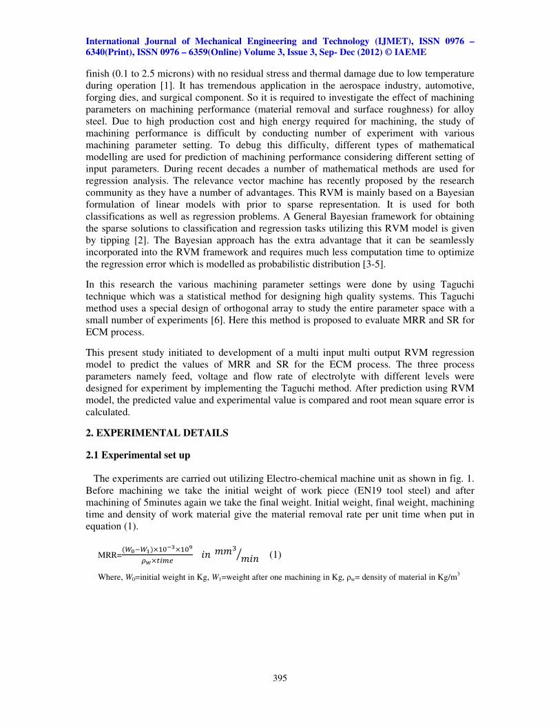
The experiments are carried out utilizing Electro-chemical machine unit as shown in fig. 1.

Before machining we take the initial weight of work piece (EN19 tool steel) and after

machining of 5minutes again we take the final weight. Initial weight, final weight, machining

time and density of work material give the material removal rate per unit time when put in

equation (1).

MRR=(��)×�

�×��

�×��

�

�� (1)

Where, W0=initial weight in Kg, W1=weight after one machining in Kg, ρw= density of material in Kg/m3



396

And after the end of each machining we have measured the surface roughness.

Material removal based on anodic dissolution and the electrolyte flows between the

electrodes and carries away the dissolved metal. In this process, a low voltage is applied

across two electrodes as per the settings given in table 3 with a small gap size (0.1 mm – 0.5

mm) and with a high current density around 2000 A/cm2. A cylindrical type with hexagonal

head copper electrode is employed for conducting the experiment. An electrolyte, typically

NaCl dissolved with water (0.25Kg/lt.) is supplied to flow through the gap with a required

velocity setting as given in table 3. Surface roughness were measured after each machining

by using a portable stylus type profile meter, Talysurf with sample length 0.8mm, filter 2 CR,

evaluation length 4mm and traverse speed 1mm/Sec. The work piece (EN19) material

composition and mechanical properties are shown in Table 1 and Table 2 respectively. All

the response parameters, MRR and SR are tabulated after experiments.

Table 1 Chemical composition of work piece material in percentage by weight

Work

piece

material

Chemical proportion in percentage of weight

C Mn P S Si Cr Mo

EN19

steel

0.38-0.43 0.75-1.00 0.035 0.04 0.15-0.3 0.8-1.10 0.15-0.25

Table 2 The mechanical characteristic of work piece material

Mechanical Properties

Density (Kg/m3) 7.7×10

3

Poisson’s ratio 0.27-0.3

Elastic Modulus

(GPA) 190-210

Hardness (HB) 197

Figure 1 Electro-chemical machining unit for conducting Experiment



397

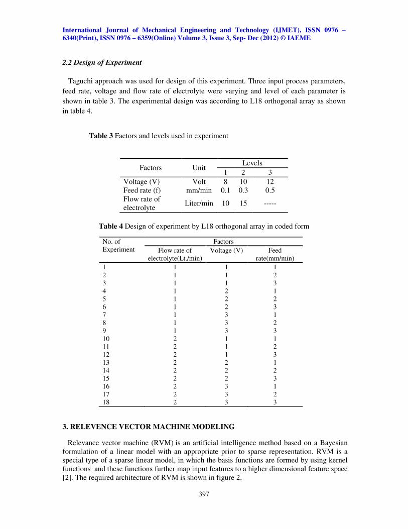
2.2 Design of Experiment

Taguchi approach was used for design of this experiment. Three input process parameters,

feed rate, voltage and flow rate of electrolyte were varying and level of each parameter is

shown in table 3. The experimental design was according to L18 orthogonal array as shown

in table 4.

Table 3 Factors and levels used in experiment

Table 4 Design of experiment by L18 orthogonal array in coded form

No. of

Experiment

Factors

Flow rate of

electrolyte(Lt./min)

Voltage (V) Feed

rate(mm/min)

1 1 1 1

2 1 1 2

3 1 1 3

4 1 2 1

5 1 2 2

6 1 2 3

7 1 3 1

8 1 3 2

9 1 3 3

10 2 1 1

11 2 1 2

12 2 1 3

13 2 2 1

14 2 2 2

15 2 2 3

16 2 3 1

17 2 3 2

18 2 3 3

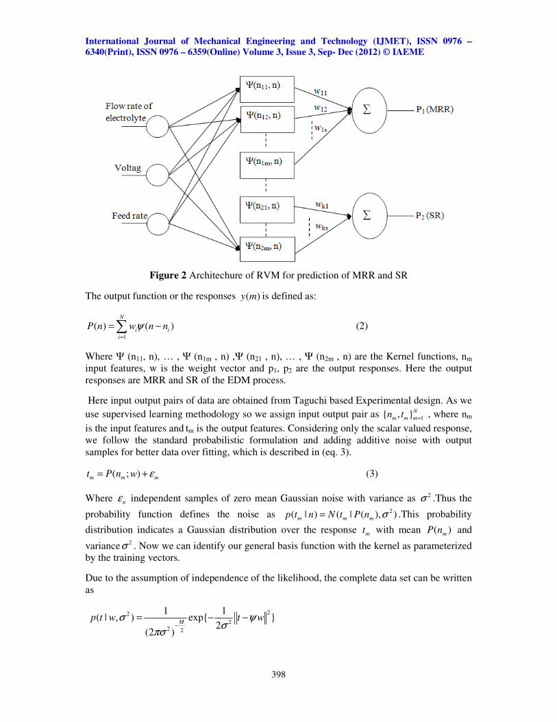
3. RELEVENCE VECTOR MACHINE MODELING

Relevance vector machine (RVM) is an artificial intelligence method based on a Bayesian

formulation of a linear model with an appropriate prior to sparse representation. RVM is a

special type of a sparse linear model, in which the basis functions are formed by using kernel

functions and these functions further map input features to a higher dimensional feature space

[2]. The required architecture of RVM is shown in figure 2.

Factors Unit Levels

1 2 3

Voltage (V) Volt 8 10 12

Feed rate (f) mm/min 0.1 0.3 0.5

Flow rate of

electrolyte Liter/min 10 15 -----

International Journal of Mechanical Engineering and Technology (IJMET), ISSN 0976

6340(Print), ISSN 0976 – 6359(Online) Volume 3, Issue 3, Sep

Figure 2 Architechure of RVM for prediction of MRR and SR

The output function or the responses

1

( ) ( )N

i i

i

P n w n nψ=

= −∑

Where Ψ (n11, n), … , Ψ (n1m ,

input features, w is the weight vector and p

responses are MRR and SR of the EDM proce

Here input output pairs of data are

use supervised learning methodology so we assign input output pair as

is the input features and tm is the output

we follow the standard probabilistic formulation and adding additive noise with output

samples for better data over fitting, which is described in (eq. 3).

( ; )m m mt P n w ε= +

Where nε independent samples

probability function defines the noise as

distribution indicates a Gaussian distribution over the

variance 2σ . Now we can identify our general basis function with the kernel as parameterized

by the training vectors.

Due to the assumption of independence of the likeliho

as

2

2 2

1 1( | , ) exp{ }

2(2 )

Mp t w t wσ ψ

πσ−

= − −


6359(Online) Volume 3, Issue 3, Sep- Dec (2012) © IAEME

398

Architechure of RVM for prediction of MRR and SR

or the responses ( )y m is defined as:

(2)

, n) ,Ψ (n21 , n), … , Ψ (n2m , n) are the Kernel functions

input features, w is the weight vector and p1, p2 are the output responses. Here the output

of the EDM process.

of data are obtained from Taguchi based Experimental design. As we

use supervised learning methodology so we assign input output pair as { , }N

m m mn t

is the output features. Considering only the scalar valued

follow the standard probabilistic formulation and adding additive noise with output

samples for better data over fitting, which is described in (eq. 3).

(3)

independent samples of zero mean Gaussian noise with variance as

probability function defines the noise as 2( | ) ( | ( ), )

m m mp t n N t P n σ= .This probability

a Gaussian distribution over the response mt with mean

. Now we can identify our general basis function with the kernel as parameterized

of independence of the likelihood, the complete data set can be written

2

2

1 1( | , ) exp{ }

2p t w t wσ ψ

σ= − −


Dec (2012) © IAEME

Kernel functions, nm

are the output responses. Here the output

Taguchi based Experimental design. As we

1{ , }N

m m m= , where nm

only the scalar valued response,

follow the standard probabilistic formulation and adding additive noise with output

(3)

as 2σ .Thus the

his probability

with mean ( )mP n and

. Now we can identify our general basis function with the kernel as parameterized

od, the complete data set can be written



399

Where1( ,.......... )T

Mt t t= are the output vectors,

0( ,....... )T

Mw w w= are weight vectors and ψ is

the ( 1)M M× + design matrix.

1 2( ) [1, ( , ), ( , )............. ( , )]T

m m m m Mn K n n K n n K n nψ =

The different process parameters in the RVM model are obtained from training examples are w and 2σ however we expect a optimise value for both w and

2σ for better prediction of MRR and

SR for testing data.

In RVM model, we follow the Bayesian prior probability distribution to modify previous

probabilistic approach. First, we must encode a preference for smoother functions by making the

popular choice of a zero-mean Gaussian prior distribution over w . The distribution given in (eq-

4)

1

0

( / ) ( | 0, )M

i i

i

p w N wα α −

=

= ∏ (4)

Where α is the vector of N+1 hyperparameters. These hyperparameters are mainly associated

with every weight between hidden feature and output. The Bayesian inference proceeds by

calculating from Bay’s rule, which is given by

2 22 ( | , , ) ( , , )

( , , | )( )

p t w p wp w t

p t

α σ α σα σ =

(5)

The new test point from testing data *n can be predicted with respect to target *t in terms of

predictive distribution as

2 2 2

* *( | ) ( | , , ) ( , , | )p t t p t w p w t dwd dα σ α σ α σ= ∫ (6)

The second term in the integral in eq-6 is called as posterior distribution over weight which is

given by

( )( )

( )2

1/2 12 ( 1)/2

2

| , ( | ) 1| , , (2 ) exp ( )

( | , ) 2

TMp t w p w

p wt w wp t

σ αα σ π µ µ

α σ

− −− + = = − − −

∑ ∑ (7)

The posterior covariance term obtained as

2 1( )TФ Ф Aσ − −= +∑ (8)

2 TФ tµ σ −= ∑ (9)

With 0 1 2( , , , .. )MA diag α α α α= ………

Relevance vector machine method is a machine learning procedure to search for the

best hyperparameters in posterior mode i.e. the maximization of 2( , | )p tα σ Proportional to 2 2( | , ) ( ) ( )p t p pα σ α σ with respect to α and β , in case of the uniform hyper priors we need

to maximize the term 2( | , )p t α σ .The maximization term can be computed as:



400

2 2 /2 2 1 1/2 2 1 11( | , ) ( | , ) ( | ) (2 ) | | exp{ ( ) }

2

N T T Tp t p t w p w dw I A t I A tα σ σ α π σ ψ ψ σ ψ ψ− − − − −= = + − +∫ (10)

The Values of α and �2 are obtained by maximize the (eq-10)

For α, we differentiate the (eq.10) and then equating to zero. Finally we got

2

new i

i

i

γα

µ= (11)

Where iµ is the ith

posterior mean weight and we can define the quantities iγ as

1i i iiγ α≡ − ∑ (12)

Where the ii∑ the i

th diagonal element of the posterior weight covariance from (eq-8) computed

with the current α and 2σ values. For the noise variance

2σ , this differentiation leads to the re-

estimate the variance as

22

( )new

ii

t Ф

M

µσ

γ

−=

−∑

(13)

Where M in the denominator refers to the number of data examples.

For this convergence of the hyperparameter estimation procedure, we have to make

predictions based on the posterior distribution over the weights, in which the condition of the

maximizing values are MPα and 2

MPσ .We can then compute the predictive distribution, from

(eq-6), for a new data m* by using(7):

( ) ( ) ( )2 2 2

* * ,| , , | , | ,MP MP MP MP MP

p t t p t w p w t dwα σ σ α σ= ∫ (14)

As both terms in the integral are Gaussian, so we can compute

( )2 2

* * * *| , , ( | , )MP MP

p t t t yα σ σ= N (15)

With final value as

* *( )TP nµ ψ= (16)

2 2

* * *( ) ( )T

MPn nσ σ ψ ψ= + ∑ (17)

So the prediction of the normalized valued as *( ; )P n µ and which can be computed by

taking the normalized value of 2

*σ and *( )nψ .

4. RESULT AND DISCUSSION

The design for the experiment was carried out with the help of machining parameters

like flow rate of electrolyte, voltage and feed rate by Taguchi technique using MINTAB 16.

The experimental result for material removal rate and surface roughness were tabulated in

table 5 with process parameters at different level in coded form.



401

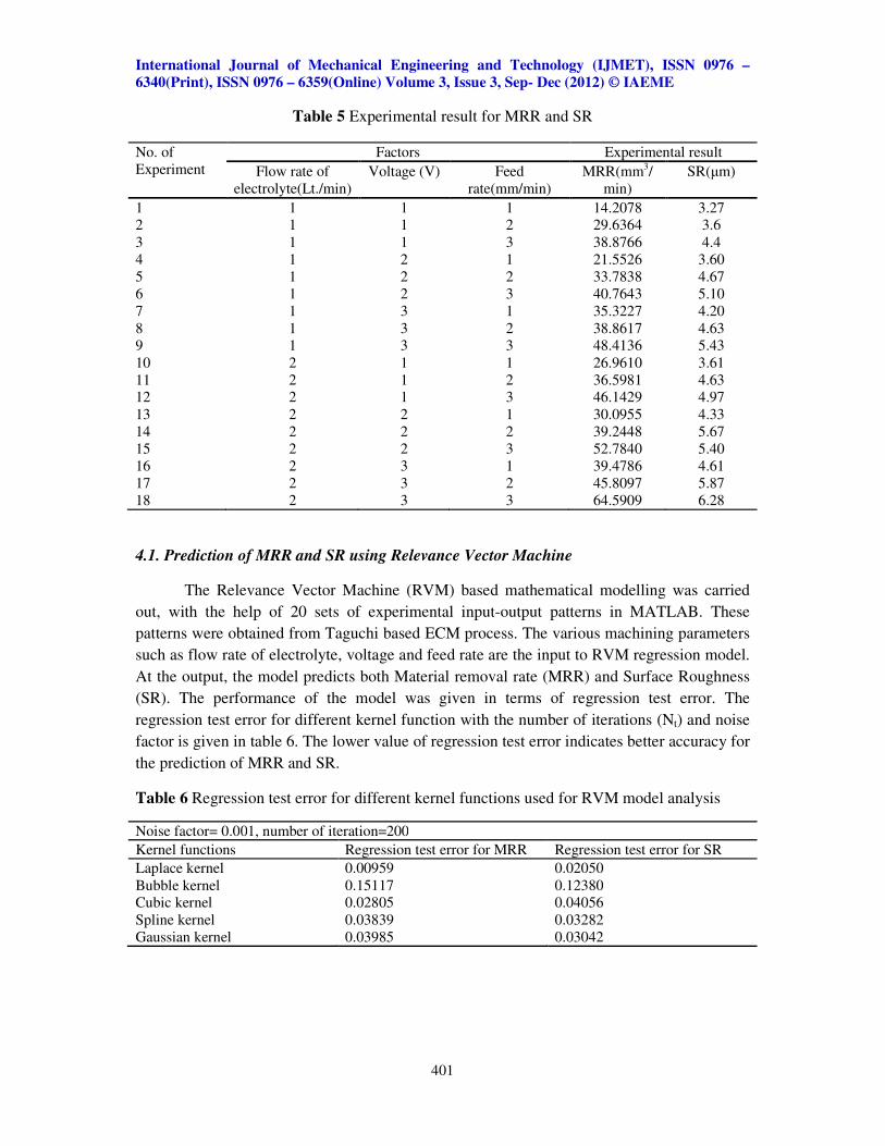
Table 5 Experimental result for MRR and SR

No. of

Experiment

Factors Experimental result

Flow rate of

electrolyte(Lt./min)

Voltage (V) Feed

rate(mm/min)

MRR(mm3/

min)

SR(µm)

1 1 1 1 14.2078 3.27

2 1 1 2 29.6364 3.6

3 1 1 3 38.8766 4.4

4 1 2 1 21.5526 3.60

5 1 2 2 33.7838 4.67

6 1 2 3 40.7643 5.10

7 1 3 1 35.3227 4.20

8 1 3 2 38.8617 4.63

9 1 3 3 48.4136 5.43

10 2 1 1 26.9610 3.61

11 2 1 2 36.5981 4.63

12 2 1 3 46.1429 4.97

13 2 2 1 30.0955 4.33

14 2 2 2 39.2448 5.67

15 2 2 3 52.7840 5.40

16 2 3 1 39.4786 4.61

17 2 3 2 45.8097 5.87

18 2 3 3 64.5909 6.28

4.1. Prediction of MRR and SR using Relevance Vector Machine

The Relevance Vector Machine (RVM) based mathematical modelling was carried

out, with the help of 20 sets of experimental input-output patterns in MATLAB. These

patterns were obtained from Taguchi based ECM process. The various machining parameters

such as flow rate of electrolyte, voltage and feed rate are the input to RVM regression model.

At the output, the model predicts both Material removal rate (MRR) and Surface Roughness

(SR). The performance of the model was given in terms of regression test error. The

regression test error for different kernel function with the number of iterations (Nt) and noise

factor is given in table 6. The lower value of regression test error indicates better accuracy for

the prediction of MRR and SR.

Table 6 Regression test error for different kernel functions used for RVM model analysis

Noise factor= 0.001, number of iteration=200

Kernel functions Regression test error for MRR Regression test error for SR

Laplace kernel 0.00959 0.02050

Bubble kernel 0.15117 0.12380

Cubic kernel 0.02805 0.04056

Spline kernel 0.03839 0.03282

Gaussian kernel 0.03985 0.03042


6340(Print), ISSN 0976 – 6359(Online) Volume 3, Issue 3, Sep

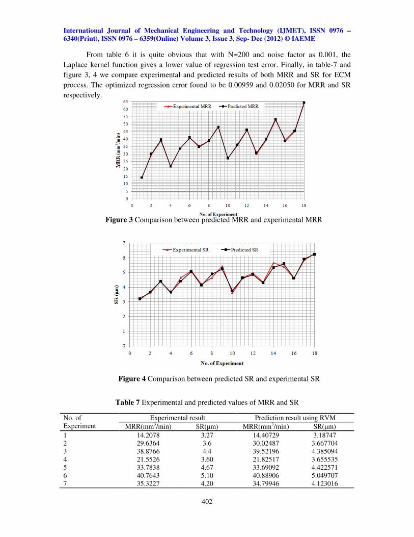
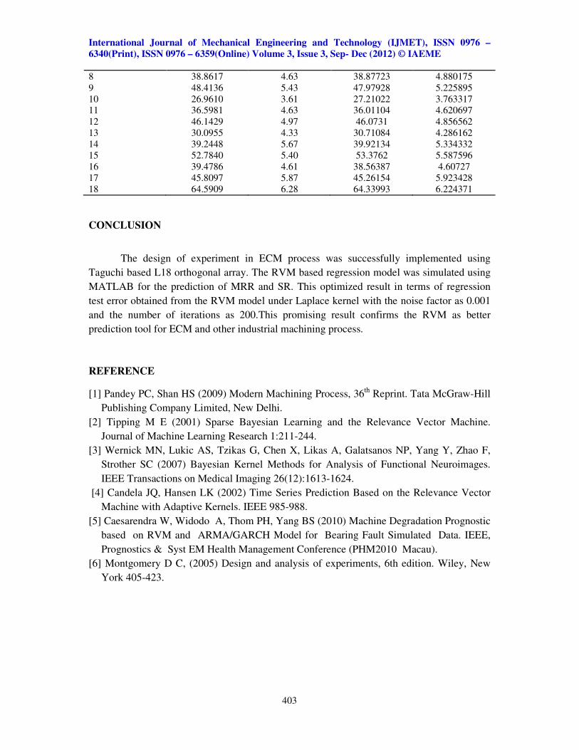
From table 6 it is quite obvious that with N=200 and noise factor as 0.001, the

Laplace kernel function gives a lower value of regression test error. Fina

figure 3, 4 we compare experimental and predicted results of both MRR and SR for ECM

process. The optimized regression error found to be 0.00959 and 0.02050 for MRR and SR

respectively.

Table 7 Experimental and pre

No. of

Experiment

Experimental result

MRR(mm3/min)

1 14.2078

2 29.6364

3 38.8766

4 21.5526

5 33.7838

6 40.7643

7 35.3227

Figure 3 Comparison between predicted MRR and experimental MRR

Figure 4 Comparison between predicted SR and experimental SR


6359(Online) Volume 3, Issue 3, Sep- Dec (2012) © IAEME

402


Laplace kernel function gives a lower value of regression test error. Finally, in table

we compare experimental and predicted results of both MRR and SR for ECM


Experimental and predicted values of MRR and SR

Experimental result Prediction result using RVM

/min) SR(µm) MRR(mm3/min)

3.27 14.40729

3.6 30.02487

4.4 39.52196

3.60 21.82517

4.67 33.69092

5.10 40.88906

4.20 34.79946

Comparison between predicted MRR and experimental MRR

Comparison between predicted SR and experimental SR


Dec (2012) © IAEME


lly, in table-7 and

we compare experimental and predicted results of both MRR and SR for ECM


Prediction result using RVM

SR(µm)

3.18747

3.667704

4.385094

3.655535

4.422571

5.049707

4.123016

Comparison between predicted MRR and experimental MRR

Comparison between predicted SR and experimental SR



403

8 38.8617 4.63 38.87723 4.880175

9 48.4136 5.43 47.97928 5.225895

10 26.9610 3.61 27.21022 3.763317

11 36.5981 4.63 36.01104 4.620697

12 46.1429 4.97 46.0731 4.856562

13 30.0955 4.33 30.71084 4.286162

14 39.2448 5.67 39.92134 5.334332

15 52.7840 5.40 53.3762 5.587596

16 39.4786 4.61 38.56387 4.60727

17 45.8097 5.87 45.26154 5.923428

18 64.5909 6.28 64.33993 6.224371

CONCLUSION

The design of experiment in ECM process was successfully implemented using

Taguchi based L18 orthogonal array. The RVM based regression model was simulated using

MATLAB for the prediction of MRR and SR. This optimized result in terms of regression

test error obtained from the RVM model under Laplace kernel with the noise factor as 0.001

and the number of iterations as 200.This promising result confirms the RVM as better

prediction tool for ECM and other industrial machining process.

REFERENCE

[1] Pandey PC, Shan HS (2009) Modern Machining Process, 36th

Reprint. Tata McGraw-Hill

Publishing Company Limited, New Delhi.

[2] Tipping M E (2001) Sparse Bayesian Learning and the Relevance Vector Machine.

Journal of Machine Learning Research 1:211-244.

[3] Wernick MN, Lukic AS, Tzikas G, Chen X, Likas A, Galatsanos NP, Yang Y, Zhao F,

Strother SC (2007) Bayesian Kernel Methods for Analysis of Functional Neuroimages.

IEEE Transactions on Medical Imaging 26(12):1613-1624.

[4] Candela JQ, Hansen LK (2002) Time Series Prediction Based on the Relevance Vector

Machine with Adaptive Kernels. IEEE 985-988.

[5] Caesarendra W, Widodo A, Thom PH, Yang BS (2010) Machine Degradation Prognostic

based on RVM and ARMA/GARCH Model for Bearing Fault Simulated Data. IEEE,

Prognostics & Syst EM Health Management Conference (PHM2010 Macau).

[6] Montgomery D C, (2005) Design and analysis of experiments, 6th edition. Wiley, New

York 405-423.

Documents

Relevance vector machine based prediction of mrrand sr for electro chemical machining process