Embed Size (px)
Citation preview

msmtools DocumentationRelease 1.2.4+0.g54dc76d.dirty
CMB group
Nov 12, 2018


Contents
1 Documentation 31.1 Installation . . . . . . . . . . . . . . . . . . . . . . . . . . . . . . . . . . . . . . . . . . . . . . . . 31.2 Documentation . . . . . . . . . . . . . . . . . . . . . . . . . . . . . . . . . . . . . . . . . . . . . . 5
2 Development 692.1 Changelog . . . . . . . . . . . . . . . . . . . . . . . . . . . . . . . . . . . . . . . . . . . . . . . . 692.2 Developer’s Guide . . . . . . . . . . . . . . . . . . . . . . . . . . . . . . . . . . . . . . . . . . . . 70
3 Indices and tables 75
Python Module Index 77
i

ii
msmtools Documentation, Release 1.2.4+0.g54dc76d.dirty
MSMTools is a Python library for the estimation, validation and analysis Markov state models.
It supports the following main features:
• Markov state model (MSM) estimation and validation.
• Computing Metastable states and structures with Perron-cluster cluster analysis (PCCA).
• Systematic coarse-graining of MSMs to transition models with few states.
• Extensive analysis options for MSMs, e.g. calculation of committors, mean first passage times, transition rates,experimental expectation values and time-correlation functions, etc.
• Transition Path Theory (TPT).
For a high-level interface to these functionalities, we encourage you to use PyEMMA.
Technical features:
• Code is implemented in Python (supports 2.7, 3.3/3.4) and C.
• Runs on Linux (64 bit), Windows (32 or 64 bit) or MacOS (64 bit).
Contents 1

msmtools Documentation, Release 1.2.4+0.g54dc76d.dirty
2 Contents
CHAPTER 1
Documentation
1.1 Installation
To install the msmtools Python package, you need a few Python package dependencies. If these dependencies are notavailable in their required versions, the installation will fail. We recommend one particular way for the installationthat is relatively safe, but you are welcome to try another approaches if you know what you are doing.
1.1.1 Anaconda install (Recommended)
We strongly recommend to use the Anaconda scientific python distribution in order to install python-based software,including msmtools. Python-based software is not trivial to distribute and this approach saves you many headachesand problems that frequently arise in other installation methods. You are free to use a different approach (see below)if you know how to sort out problems, but play at your own risk.
If you already have a conda installation, directly go to step 3:
1. Download and install miniconda for Python 2 or 3, 32 or 64 bit depending on your system: http://conda.pydata.org/miniconda.html
For Windows users, who do not know what to choose for 32 or 64 bit, it is strongly recommended to read thesecond question of this FAQ first: http://windows.microsoft.com/en-us/windows/32-bit-and-64-bit-windows
Run the installer and select yes to add conda to the PATH variable.
2. If you have installed from a Linux shell, either open a new shell to have an updated PATH, or update your PATHvariable by source ~/.bashrc (or .tcsh, .csh - whichever shell you are using).
3. Add the omnia-md software channel, and install (or update) msmtools:
conda config --add channels omniaconda install msmtools
if the command conda is unknown, the PATH variable is probably not set correctly (see 1. and 2.)
4. Check installation:
3

msmtools Documentation, Release 1.2.4+0.g54dc76d.dirty
conda list
shows you the installed python packages. You should find a msmtools 1.1 (or later) and ipython, ipython-notebook 3.1 (or later). If ipython is not up to date, you can still use msmtools, but you won’t be able to loadour example notebooks. In that case, update it by
conda install ipython-notebook
1.1.2 Python Package Index (PyPI)
If you do not like Anaconda for some reason you should use the Python package manager pip to install. This is notrecommended, because in the past, various problems have arisen with pip in compiling the packages that msmtoolsdepends upon.
1. If you do not have pip, please read the install guide: install guide.
2. Make sure pip is enabled to install so called wheel packages:
pip install wheel
Now you are able to install binaries if you use MacOSX or Windows. At the moment of writing PyPI does notsupport Linux binaries at all, so Linux users have to compile by themselves.
3. Install msmtools using
pip install msmtools
4. Check your installation
python>>> import msmtools>>> msmtools.__version__
should print 1.1 or later
>>> import IPython>>> IPython.__version__
should print 3.1 or later. If ipython is not up to date, update it by pip install ipython
1.1.3 Building from Source
If you refuse to use Anaconda, you will build msmtools from the source. In this approach, all msmtools dependencieswill be built from the source too. Building these from source is sometimes (if not usually) tricky, takes a long time andis error prone - though it is not recommended nor supported by us. If unsure, use the anaconda installation.
1. Ensure that you fulfill the following prerequisites. You can install either with pip or conda, as long as you metthe version requirements.
• C/C++ compiler
• setuptools > 18
• cython >= 0.22
• numpy >= 1.6
4 Chapter 1. Documentation

msmtools Documentation, Release 1.2.4+0.g54dc76d.dirty
• scipy >= 0.11
If you do not fulfill these requirements, try to upgrade all packages:
pip install --upgrade setuptoolspip install --upgrade cythonpip install --upgrade numpypip install --upgrade scipy
Note that if pip finds a newer version, it will trigger an update which will most likely involve compilation.Especially NumPy and SciPy are hard to build. You might want to take a look at this guide here: http://www.scipy.org/scipylib/building/
2. The build and install process is in one step, as all dependencies are dragged in via the provided setup.py script. Soyou only need to get the source of Emma and run it to build Emma itself and all of its dependencies (if not alreadysupplied) from source.
pip install msmtools
1.1.4 For Developers
If you are a developer, clone the code repository from GitHub and install it as follows
1. Ensure the prerequisites (point 1) described for “Building from Source” above.
2. Make a suitable directory, and inside clone the repository via
git clone https://github.com/markovmodel/msmtools.git
3. install msmtools via
python setup.py develop [--user]
The develop install has the advantage that if only python scripts are being changed e.g. via an pull or a localedit, you do not have to re-install anything, because the setup command simply created a link to your workingcopy. Repeating point 3 is only necessary if any of msmtools C-files change and need to be rebuilt.
1.2 Documentation
msmtools provides these packages to perform estimation and further analysis of Markov models.
1.2.1 estimation - MSM estimation from data (msmtools.estimation)
Countmatrix
count_matrix(dtraj, lag[, sliding, . . . ]) Generate a count matrix from given microstate trajec-tory.
cmatrix(dtraj, lag[, sliding, . . . ]) Generate a count matrix from given microstate trajec-tory.
1.2. Documentation 5

msmtools Documentation, Release 1.2.4+0.g54dc76d.dirty
msmtools.estimation.count_matrix
msmtools.estimation.count_matrix(dtraj, lag, sliding=True, sparse_return=True, nstates=None)Generate a count matrix from given microstate trajectory.
Parameters
• dtraj (array_like or list of array_like) – Discretized trajectory or list ofdiscretized trajectories
• lag (int) – Lagtime in trajectory steps
• sliding (bool, optional) – If true the sliding window approach is used for transi-tion counting.
• sparse_return (bool (optional)) – Whether to return a dense or a sparse matrix.
• nstates (int, optional) – Enforce a count-matrix with shape=(nstates, nstates)
Returns C – The count matrix at given lag in coordinate list format.
Return type scipy.sparse.coo_matrix
Notes
Transition counts can be obtained from microstate trajectory using two methods. Couning at lag and sliding-window counting.
Lag
This approach will skip all points in the trajectory that are seperated form the last point by less than the givenlagtime 𝜏 .
Transition counts 𝑐𝑖𝑗(𝜏) are generated according to
𝑐𝑖𝑗(𝜏) =
⌊𝑁𝜏 ⌋−2∑𝑘=0
𝜒𝑖(𝑋𝑘𝜏 )𝜒𝑗(𝑋(𝑘+1)𝜏 ).
𝜒𝑖(𝑥) is the indicator function of 𝑖, i.e 𝜒𝑖(𝑥) = 1 for 𝑥 = 𝑖 and 𝜒𝑖(𝑥) = 0 for 𝑥 = 𝑖.
Sliding
The sliding approach slides along the trajectory and counts all transitions sperated by the lagtime 𝜏 .
Transition counts 𝑐𝑖𝑗(𝜏) are generated according to
𝑐𝑖𝑗(𝜏) =
𝑁−𝜏−1∑𝑘=0
𝜒𝑖(𝑋𝑘)𝜒𝑗(𝑋𝑘+𝜏 ).
References
Examples
>>> import numpy as np>>> from msmtools.estimation import count_matrix
6 Chapter 1. Documentation

msmtools Documentation, Release 1.2.4+0.g54dc76d.dirty
>>> dtraj = np.array([0, 0, 1, 0, 1, 1, 0])>>> tau = 2
Use the sliding approach first
>>> C_sliding = count_matrix(dtraj, tau)
The generated matrix is a sparse matrix in CSR-format. For convenient printing we convert it to a dense ndarray.
>>> C_sliding.toarray()array([[ 1., 2.],
[ 1., 1.]])
Let us compare to the count-matrix we obtain using the lag approach
>>> C_lag = count_matrix(dtraj, tau, sliding=False)>>> C_lag.toarray()array([[ 0., 1.],
[ 1., 1.]])
msmtools.estimation.cmatrix
msmtools.estimation.cmatrix(dtraj, lag, sliding=True, sparse_return=True, nstates=None)Generate a count matrix from given microstate trajectory.
Parameters
• dtraj (array_like or list of array_like) – Discretized trajectory or list ofdiscretized trajectories
• lag (int) – Lagtime in trajectory steps
• sliding (bool, optional) – If true the sliding window approach is used for transi-tion counting.
• sparse_return (bool (optional)) – Whether to return a dense or a sparse matrix.
• nstates (int, optional) – Enforce a count-matrix with shape=(nstates, nstates)
Returns C – The count matrix at given lag in coordinate list format.
Return type scipy.sparse.coo_matrix
Notes
Transition counts can be obtained from microstate trajectory using two methods. Couning at lag and sliding-window counting.
Lag
This approach will skip all points in the trajectory that are seperated form the last point by less than the givenlagtime 𝜏 .
Transition counts 𝑐𝑖𝑗(𝜏) are generated according to
𝑐𝑖𝑗(𝜏) =
⌊𝑁𝜏 ⌋−2∑𝑘=0
𝜒𝑖(𝑋𝑘𝜏 )𝜒𝑗(𝑋(𝑘+1)𝜏 ).
1.2. Documentation 7

msmtools Documentation, Release 1.2.4+0.g54dc76d.dirty
𝜒𝑖(𝑥) is the indicator function of 𝑖, i.e 𝜒𝑖(𝑥) = 1 for 𝑥 = 𝑖 and 𝜒𝑖(𝑥) = 0 for 𝑥 = 𝑖.
Sliding
The sliding approach slides along the trajectory and counts all transitions sperated by the lagtime 𝜏 .
Transition counts 𝑐𝑖𝑗(𝜏) are generated according to
𝑐𝑖𝑗(𝜏) =
𝑁−𝜏−1∑𝑘=0
𝜒𝑖(𝑋𝑘)𝜒𝑗(𝑋𝑘+𝜏 ).
References
Examples
>>> import numpy as np>>> from msmtools.estimation import count_matrix
>>> dtraj = np.array([0, 0, 1, 0, 1, 1, 0])>>> tau = 2
Use the sliding approach first
>>> C_sliding = count_matrix(dtraj, tau)
The generated matrix is a sparse matrix in CSR-format. For convenient printing we convert it to a dense ndarray.
>>> C_sliding.toarray()array([[ 1., 2.],
[ 1., 1.]])
Let us compare to the count-matrix we obtain using the lag approach
>>> C_lag = count_matrix(dtraj, tau, sliding=False)>>> C_lag.toarray()array([[ 0., 1.],
[ 1., 1.]])
Connectivity
connected_sets(C[, directed]) Compute connected sets of microstates.largest_connected_set(C[, directed]) Largest connected component for a directed graph with
edge-weights given by the count matrix.largest_connected_submatrix(C[, directed,lcc])
Compute the count matrix on the largest connected set.
connected_cmatrix(C[, directed, lcc]) Compute the count matrix on the largest connected set.is_connected(C[, directed]) Check connectivity of the given matrix.
msmtools.estimation.connected_sets
msmtools.estimation.connected_sets(C, directed=True)Compute connected sets of microstates.
8 Chapter 1. Documentation

msmtools Documentation, Release 1.2.4+0.g54dc76d.dirty
Connected components for a directed graph with edge-weights given by the count matrix.
Parameters
• C (scipy.sparse matrix) – Count matrix specifying edge weights.
• directed (bool, optional) – Whether to compute connected components for a di-rected or undirected graph. Default is True.
Returns cc – Each entry is an array containing all vertices (states) in the corresponding connectedcomponent. The list is sorted according to the size of the individual components. The largestconnected set is the first entry in the list, lcc=cc[0].
Return type list of arrays of integers
Notes
Viewing the count matrix as the adjacency matrix of a (directed) graph the connected components are given bythe connected components of that graph. Connected components of a graph can be efficiently computed usingTarjan’s algorithm.
References
Examples
>>> import numpy as np>>> from msmtools.estimation import connected_sets
>>> C = np.array([[10, 1, 0], [2, 0, 3], [0, 0, 4]])>>> cc_directed = connected_sets(C)>>> cc_directed[array([0, 1]), array([2])]
>>> cc_undirected = connected_sets(C, directed=False)>>> cc_undirected[array([0, 1, 2])]
msmtools.estimation.largest_connected_set
msmtools.estimation.largest_connected_set(C, directed=True)Largest connected component for a directed graph with edge-weights given by the count matrix.
Parameters
• C (scipy.sparse matrix) – Count matrix specifying edge weights.
• directed (bool, optional) – Whether to compute connected components for a di-rected or undirected graph. Default is True.
Returns lcc – The largest connected component of the directed graph.
Return type array of integers
See also:
connected_sets()
1.2. Documentation 9

msmtools Documentation, Release 1.2.4+0.g54dc76d.dirty
Notes
Viewing the count matrix as the adjacency matrix of a (directed) graph the largest connected set is the largestconnected set of nodes of the corresponding graph. The largest connected set of a graph can be efficientlycomputed using Tarjan’s algorithm.
References
Examples
>>> import numpy as np>>> from msmtools.estimation import largest_connected_set
>>> C = np.array([[10, 1, 0], [2, 0, 3], [0, 0, 4]])>>> lcc_directed = largest_connected_set(C)>>> lcc_directedarray([0, 1])
>>> lcc_undirected = largest_connected_set(C, directed=False)>>> lcc_undirectedarray([0, 1, 2])
msmtools.estimation.largest_connected_submatrix
msmtools.estimation.largest_connected_submatrix(C, directed=True, lcc=None)Compute the count matrix on the largest connected set.
Parameters
• C (scipy.sparse matrix) – Count matrix specifying edge weights.
• directed (bool, optional) – Whether to compute connected components for a di-rected or undirected graph. Default is True
• lcc ((M,) ndarray, optional) – The largest connected set
Returns C_cc – Count matrix of largest completely connected set of vertices (states)
Return type scipy.sparse matrix
See also:
largest_connected_set()
Notes
Viewing the count matrix as the adjacency matrix of a (directed) graph the larest connected submatrix is theadjacency matrix of the largest connected set of the corresponding graph. The largest connected submatrix canbe efficiently computed using Tarjan’s algorithm.
10 Chapter 1. Documentation

msmtools Documentation, Release 1.2.4+0.g54dc76d.dirty
References
Examples
>>> import numpy as np>>> from msmtools.estimation import largest_connected_submatrix
>>> C = np.array([[10, 1, 0], [2, 0, 3], [0, 0, 4]])
>>> C_cc_directed = largest_connected_submatrix(C)>>> C_cc_directedarray([[10, 1],
[ 2, 0]]...)
>>> C_cc_undirected = largest_connected_submatrix(C, directed=False)>>> C_cc_undirectedarray([[10, 1, 0],
[ 2, 0, 3],[ 0, 0, 4]]...)
msmtools.estimation.connected_cmatrix
msmtools.estimation.connected_cmatrix(C, directed=True, lcc=None)Compute the count matrix on the largest connected set.
Parameters
• C (scipy.sparse matrix) – Count matrix specifying edge weights.
• directed (bool, optional) – Whether to compute connected components for a di-rected or undirected graph. Default is True
• lcc ((M,) ndarray, optional) – The largest connected set
Returns C_cc – Count matrix of largest completely connected set of vertices (states)
Return type scipy.sparse matrix
See also:
largest_connected_set()
Notes
Viewing the count matrix as the adjacency matrix of a (directed) graph the larest connected submatrix is theadjacency matrix of the largest connected set of the corresponding graph. The largest connected submatrix canbe efficiently computed using Tarjan’s algorithm.
1.2. Documentation 11

msmtools Documentation, Release 1.2.4+0.g54dc76d.dirty
References
Examples
>>> import numpy as np>>> from msmtools.estimation import largest_connected_submatrix
>>> C = np.array([[10, 1, 0], [2, 0, 3], [0, 0, 4]])
>>> C_cc_directed = largest_connected_submatrix(C)>>> C_cc_directedarray([[10, 1],
[ 2, 0]]...)
>>> C_cc_undirected = largest_connected_submatrix(C, directed=False)>>> C_cc_undirectedarray([[10, 1, 0],
[ 2, 0, 3],[ 0, 0, 4]]...)
msmtools.estimation.is_connected
msmtools.estimation.is_connected(C, directed=True)Check connectivity of the given matrix.
Parameters
• C (scipy.sparse matrix) – Count matrix specifying edge weights.
• directed (bool, optional) – Whether to compute connected components for a di-rected or undirected graph. Default is True.
Returns is_connected – True if C is connected, False otherwise.
Return type bool
See also:
largest_connected_submatrix()
Notes
A count matrix is connected if the graph having the count matrix as adjacency matrix has a single connectedcomponent. Connectivity of a graph can be efficiently checked using Tarjan’s algorithm.
References
Examples
>>> import numpy as np>>> from msmtools.estimation import is_connected
12 Chapter 1. Documentation
msmtools Documentation, Release 1.2.4+0.g54dc76d.dirty
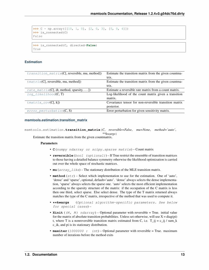
>>> C = np.array([[10, 1, 0], [2, 0, 3], [0, 0, 4]])>>> is_connected(C)False
>>> is_connected(C, directed=False)True
Estimation
transition_matrix(C[, reversible, mu, method]) Estimate the transition matrix from the given countma-trix.
tmatrix(C[, reversible, mu, method]) Estimate the transition matrix from the given countma-trix.
rate_matrix(C[, dt, method, sparsity, . . . ]) Estimate a reversible rate matrix from a count matrix.log_likelihood(C, T) Log-likelihood of the count matrix given a transition
matrix.tmatrix_cov(C[, k]) Covariance tensor for non-reversible transition matrix
posterior.error_perturbation(C, S) Error perturbation for given sensitivity matrix.
msmtools.estimation.transition_matrix
msmtools.estimation.transition_matrix(C, reversible=False, mu=None, method=’auto’,**kwargs)
Estimate the transition matrix from the given countmatrix.
Parameters
• C (numpy ndarray or scipy.sparse matrix) – Count matrix
• reversible (bool (optional)) – If True restrict the ensemble of transition matricesto those having a detailed balance symmetry otherwise the likelihood optimization is carriedout over the whole space of stochastic matrices.
• mu (array_like) – The stationary distribution of the MLE transition matrix.
• method (str) – Select which implementation to use for the estimation. One of ‘auto’,‘dense’ and ‘sparse’, optional, default=’auto’. ‘dense’ always selects the dense implementa-tion, ‘sparse’ always selects the sparse one. ‘auto’ selects the most efficient implementationaccording to the sparsity structure of the matrix: if the occupation of the C matrix is lessthen one third, select sparse. Else select dense. The type of the T matrix returned alwaysmatches the type of the C matrix, irrespective of the method that was used to compute it.
• **kwargs (Optional algorithm-specific parameters. See belowfor special cases) –
• Xinit ((M, M) ndarray) – Optional parameter with reversible = True. initial valuefor the matrix of absolute transition probabilities. Unless set otherwise, will use X = diag(pi)t, where T is a nonreversible transition matrix estimated from C, i.e. T_ij = c_ij / sum_kc_ik, and pi is its stationary distribution.
• maxiter (1000000 : int) – Optional parameter with reversible = True. maximumnumber of iterations before the method exits
1.2. Documentation 13

msmtools Documentation, Release 1.2.4+0.g54dc76d.dirty
• maxerr (1e-8 : float) – Optional parameter with reversible = True. convergencetolerance for transition matrix estimation. This specifies the maximum change of the Eu-clidean norm of relative stationary probabilities (𝑥𝑖 =
∑𝑘 𝑥𝑖𝑘). The relative stationary
probability changes 𝑒𝑖 = (𝑥(1)𝑖 − 𝑥
(2)𝑖 )/(𝑥
(1)𝑖 + 𝑥
(2)𝑖 ) are used in order to track changes in
small probabilities. The Euclidean norm of the change vector, |𝑒𝑖|2, is compared to maxerr.
• rev_pisym (bool, default=False) – Fast computation of reversible transition ma-trix by normalizing 𝑥𝑖𝑗 = 𝜋𝑖𝑝𝑖𝑗 + 𝜋𝑗𝑝𝑗𝑖. 𝑝𝑖𝑗 is the direct (nonreversible) estimate and 𝑝𝑖𝑖is its stationary distribution. This estimator is asympotically unbiased but not maximumlikelihood.
• return_statdist (bool, default=False) – Optional parameter with reversible= True. If set to true, the stationary distribution is also returned
• return_conv (bool, default=False) – Optional parameter with reversible =True. If set to true, the likelihood history and the pi_change history is returned.
• warn_not_converged (bool, default=True) – Prints a warning if not con-verged.
• sparse_newton (bool, default=False) – If True, use the experimental primal-dual interior-point solver for sparse input/computation method.
Returns
• P ((M, M) ndarray or scipy.sparse matrix) – The MLE transition matrix. P has the samedata type (dense or sparse) as the input matrix C.
• The reversible estimator returns by default only P, but may also return
• (P,pi) or (P,lhist,pi_changes) or (P,pi,lhist,pi_changes) depending on the return settings
• P (ndarray (n,n)) – transition matrix. This is the only return for return_statdist = False,return_conv = False
• (pi) (ndarray (n)) – stationary distribution. Only returned if return_statdist = True
• (lhist) (ndarray (k)) – likelihood history. Has the length of the number of iterations needed.Only returned if return_conv = True
• (pi_changes) (ndarray (k)) – history of likelihood history. Has the length of the number ofiterations needed. Only returned if return_conv = True
Notes
The transition matrix is a maximum likelihood estimate (MLE) of the probability distribution of transitionmatrices with parameters given by the count matrix.
References
Examples
>>> import numpy as np>>> from msmtools.estimation import transition_matrix
>>> C = np.array([[10, 1, 1], [2, 0, 3], [0, 1, 4]])
Non-reversible estimate
14 Chapter 1. Documentation

msmtools Documentation, Release 1.2.4+0.g54dc76d.dirty
>>> T_nrev = transition_matrix(C)>>> T_nrevarray([[ 0.83333333, 0.08333333, 0.08333333],
[ 0.4 , 0. , 0.6 ],[ 0. , 0.2 , 0.8 ]])
Reversible estimate
>>> T_rev = transition_matrix(C, reversible=True)>>> T_revarray([[ 0.83333333, 0.10385551, 0.06281115],
[ 0.35074677, 0. , 0.64925323],[ 0.04925323, 0.15074677, 0.8 ]])
Reversible estimate with given stationary vector
>>> mu = np.array([0.7, 0.01, 0.29])>>> T_mu = transition_matrix(C, reversible=True, mu=mu)>>> T_muarray([[ 0.94771371, 0.00612645, 0.04615984],
[ 0.42885157, 0. , 0.57114843],[ 0.11142031, 0.01969477, 0.86888491]])
msmtools.estimation.tmatrix
msmtools.estimation.tmatrix(C, reversible=False, mu=None, method=’auto’, **kwargs)Estimate the transition matrix from the given countmatrix.
Parameters
• C (numpy ndarray or scipy.sparse matrix) – Count matrix
• reversible (bool (optional)) – If True restrict the ensemble of transition matricesto those having a detailed balance symmetry otherwise the likelihood optimization is carriedout over the whole space of stochastic matrices.
• mu (array_like) – The stationary distribution of the MLE transition matrix.
• method (str) – Select which implementation to use for the estimation. One of ‘auto’,‘dense’ and ‘sparse’, optional, default=’auto’. ‘dense’ always selects the dense implementa-tion, ‘sparse’ always selects the sparse one. ‘auto’ selects the most efficient implementationaccording to the sparsity structure of the matrix: if the occupation of the C matrix is lessthen one third, select sparse. Else select dense. The type of the T matrix returned alwaysmatches the type of the C matrix, irrespective of the method that was used to compute it.
• **kwargs (Optional algorithm-specific parameters. See belowfor special cases) –
• Xinit ((M, M) ndarray) – Optional parameter with reversible = True. initial valuefor the matrix of absolute transition probabilities. Unless set otherwise, will use X = diag(pi)t, where T is a nonreversible transition matrix estimated from C, i.e. T_ij = c_ij / sum_kc_ik, and pi is its stationary distribution.
• maxiter (1000000 : int) – Optional parameter with reversible = True. maximumnumber of iterations before the method exits
• maxerr (1e-8 : float) – Optional parameter with reversible = True. convergencetolerance for transition matrix estimation. This specifies the maximum change of the Eu-
1.2. Documentation 15

msmtools Documentation, Release 1.2.4+0.g54dc76d.dirty
clidean norm of relative stationary probabilities (𝑥𝑖 =∑
𝑘 𝑥𝑖𝑘). The relative stationaryprobability changes 𝑒𝑖 = (𝑥
(1)𝑖 − 𝑥
(2)𝑖 )/(𝑥
(1)𝑖 + 𝑥
(2)𝑖 ) are used in order to track changes in
small probabilities. The Euclidean norm of the change vector, |𝑒𝑖|2, is compared to maxerr.
• rev_pisym (bool, default=False) – Fast computation of reversible transition ma-trix by normalizing 𝑥𝑖𝑗 = 𝜋𝑖𝑝𝑖𝑗 + 𝜋𝑗𝑝𝑗𝑖. 𝑝𝑖𝑗 is the direct (nonreversible) estimate and 𝑝𝑖𝑖is its stationary distribution. This estimator is asympotically unbiased but not maximumlikelihood.
• return_statdist (bool, default=False) – Optional parameter with reversible= True. If set to true, the stationary distribution is also returned
• return_conv (bool, default=False) – Optional parameter with reversible =True. If set to true, the likelihood history and the pi_change history is returned.
• warn_not_converged (bool, default=True) – Prints a warning if not con-verged.
• sparse_newton (bool, default=False) – If True, use the experimental primal-dual interior-point solver for sparse input/computation method.
Returns
• P ((M, M) ndarray or scipy.sparse matrix) – The MLE transition matrix. P has the samedata type (dense or sparse) as the input matrix C.
• The reversible estimator returns by default only P, but may also return
• (P,pi) or (P,lhist,pi_changes) or (P,pi,lhist,pi_changes) depending on the return settings
• P (ndarray (n,n)) – transition matrix. This is the only return for return_statdist = False,return_conv = False
• (pi) (ndarray (n)) – stationary distribution. Only returned if return_statdist = True
• (lhist) (ndarray (k)) – likelihood history. Has the length of the number of iterations needed.Only returned if return_conv = True
• (pi_changes) (ndarray (k)) – history of likelihood history. Has the length of the number ofiterations needed. Only returned if return_conv = True
Notes
The transition matrix is a maximum likelihood estimate (MLE) of the probability distribution of transitionmatrices with parameters given by the count matrix.
References
Examples
>>> import numpy as np>>> from msmtools.estimation import transition_matrix
>>> C = np.array([[10, 1, 1], [2, 0, 3], [0, 1, 4]])
Non-reversible estimate
16 Chapter 1. Documentation

msmtools Documentation, Release 1.2.4+0.g54dc76d.dirty
>>> T_nrev = transition_matrix(C)>>> T_nrevarray([[ 0.83333333, 0.08333333, 0.08333333],
[ 0.4 , 0. , 0.6 ],[ 0. , 0.2 , 0.8 ]])
Reversible estimate
>>> T_rev = transition_matrix(C, reversible=True)>>> T_revarray([[ 0.83333333, 0.10385551, 0.06281115],
[ 0.35074677, 0. , 0.64925323],[ 0.04925323, 0.15074677, 0.8 ]])
Reversible estimate with given stationary vector
>>> mu = np.array([0.7, 0.01, 0.29])>>> T_mu = transition_matrix(C, reversible=True, mu=mu)>>> T_muarray([[ 0.94771371, 0.00612645, 0.04615984],
[ 0.42885157, 0. , 0.57114843],[ 0.11142031, 0.01969477, 0.86888491]])
msmtools.estimation.rate_matrix
msmtools.estimation.rate_matrix(C, dt=1.0, method=’KL’, sparsity=None, t_agg=None,pi=None, tol=10000000.0, K0=None, maxiter=100000,on_error=’raise’)
Estimate a reversible rate matrix from a count matrix.
Parameters
• C ((N,N) ndarray) – count matrix at a lag time dt
• dt (float, optional, default=1.0) – lag time that was used to estimate C
• method (str, one of {'KL', 'CVE', 'pseudo', 'truncated_log'}) –Method to use for estimation of the rate matrix.
– ’pseudo’ selects the pseudo-generator. A reversible transition matrix T is estimated and(𝑇 − 𝐼𝑑)/𝑑 is returned as the rate matrix.
– ’truncated_log’ selects the truncated logarithm3. A reversible transition matrix T is esti-mated and 𝑚𝑎𝑥(𝑙𝑜𝑔𝑚(𝑇 * 𝑇 )/(2𝑑𝑡), 0) is returned as the rate matrix. logm is the matrixlogarithm and the maximum is taken element-wise.
– ’CVE’ selects the algorithm of Crommelin and Vanden-Eijnden1. It consists of minimiz-ing the following objective function:
𝑓(𝐾) =∑𝑖𝑗
(∑𝑘𝑙
𝑈−1𝑖𝑘 𝐾𝑘𝑙𝑈𝑙𝑗 − 𝐿𝑖𝑗
)2
|Λ𝑖Λ𝑗 |
where Λ𝑖 are the eigenvalues of 𝑇 and 𝑈 is the matrix of its (right) eigenvectors; 𝐿𝑖𝑗 =𝛿𝑖𝑗
1𝜏 log |Λ𝑖|. 𝑇 is computed from C using the reversible maximum likelihood estimator.
3 E. B. Davies. Embeddable Markov Matrices. Electron. J. Probab. 15:1474, 2010.1 D. Crommelin and E. Vanden-Eijnden. Data-based inference of generators for markov jump processes using convex optimization. Multiscale.
Model. Sim., 7(4):1751-1778, 2009.
1.2. Documentation 17

msmtools Documentation, Release 1.2.4+0.g54dc76d.dirty
– ’KL’ selects the algorihtm of Kalbfleisch and Lawless2. It consists of maximizing thefollowing log-likelihood:
𝑓(𝐾) = log𝐿 =∑𝑖𝑗
𝐶𝑖𝑗 log(𝑒𝐾Δ𝑡)𝑖𝑗
where 𝐶𝑖𝑗 are the transition counts at a lag-time ∆𝑡. Here 𝑒 is the matrix exponential andthe logarithm is taken element-wise.
• sparsity ((N,N) ndarray or None, optional, default=None) – Ifsparsity is None, a fully occupied rate matrix will be estimated. Alternatively, with themethods ‘CVE’ and ‘KL’ a ndarray of the same shape as C can be supplied. If sparsity[i,j]=0and sparsity[j,i]=0 the rate matrix elements 𝐾𝑖𝑗 and 𝐾𝑗𝑖 will be constrained to zero.
• t_agg (float, optional) – the aggregated simulation time; by default this is the totalnumber of transition counts times the lag time (no sliding window counting). This value isused to compute the lower bound on the transition rate (that are not zero). If sparsity isNone, this value is ignored.
• pi – the stationary vector of the desired rate matrix K. If no pi is given, the function takesthe stationary vector of the MLE reversible T matrix that is computed from C.
• tol (float, optional, default = 1.0E7) – Tolerance of the quasi-Newton al-gorithm that is used to minimize the objective function. This is passed as the factr parameterto scipy.optimize.fmin_l_bfgs_b. Typical values for factr are: 1e12 for low ac-curacy; 1e7 for moderate accuracy; 10.0 for extremely high accuracy.
• maxiter (int, optional, default = 100000) – Minimization of the objectivefunction will do at most this number of steps.
• on_error (string, optional, default = 'raise') – What to do then an er-ror happend. When ‘raise’ is given, raise an exception. When ‘warn’ is given, produce a(Python) warning.
Returns K – the optimal rate matrix
Return type (N,N) ndarray
Notes
In this implementation the algorithm of Crommelin and Vanden-Eijnden (CVE) is initialized with the pseudo-generator estimate. The algorithm of Kalbfleisch and Lawless (KL) is initialized using the CVE result.
Example
>>> import numpy as np>>> from msmtools.estimation import rate_matrix>>> C = np.array([[100,1],[50,50]])>>> rate_matrix(C)array([[-0.01384753, 0.01384753],
[ 0.69930032, -0.69930032]])
2 J. D. Kalbfleisch and J. F. Lawless. The analysis of panel data under a markov assumption. J. Am. Stat. Assoc., 80(392):863-871, 1985.
18 Chapter 1. Documentation

msmtools Documentation, Release 1.2.4+0.g54dc76d.dirty
References
msmtools.estimation.log_likelihood
msmtools.estimation.log_likelihood(C, T)Log-likelihood of the count matrix given a transition matrix.
Parameters
• C ((M, M) ndarray or scipy.sparse matrix) – Count matrix
• T ((M, M) ndarray orscipy.sparse matrix) – Transition matrix
Returns logL – Log-likelihood of the count matrix
Return type float
Notes
The likelihood of a set of observed transition counts 𝐶 = (𝑐𝑖𝑗) for a given matrix of transition counts 𝑇 = (𝑡𝑖𝑗)is given by
𝐿(𝐶|𝑃 ) =
𝑀∏𝑖=1
⎛⎝ 𝑀∏𝑗=1
𝑝𝑐𝑖𝑗𝑖𝑗
⎞⎠The log-likelihood is given by
𝑙(𝐶|𝑃 ) =
𝑀∑𝑖,𝑗=1
𝑐𝑖𝑗 log 𝑝𝑖𝑗 .
The likelihood describes the probability of making an observation 𝐶 for a given model 𝑃 .
Examples
>>> import numpy as np>>> from msmtools.estimation import log_likelihood
>>> T = np.array([[0.9, 0.1, 0.0], [0.5, 0.0, 0.5], [0.0, 0.1, 0.9]])
>>> C = np.array([[58, 7, 0], [6, 0, 4], [0, 3, 21]])>>> logL = log_likelihood(C, T)>>> logL-38.2808034725...
>>> C = np.array([[58, 20, 0], [6, 0, 4], [0, 3, 21]])>>> logL = log_likelihood(C, T)>>> logL-68.2144096814...
1.2. Documentation 19

msmtools Documentation, Release 1.2.4+0.g54dc76d.dirty
References
msmtools.estimation.tmatrix_cov
msmtools.estimation.tmatrix_cov(C, k=None)Covariance tensor for non-reversible transition matrix posterior.
Parameters
• C ((M, M) ndarray or scipy.sparse matrix) – Count matrix
• k (int (optional)) – Return only covariance matrix for entires in the k-th row of thetransition matrix
Returns cov – Covariance tensor for transition matrix posterior
Return type (M, M, M) ndarray
Notes
The posterior of non-reversible transition matrices is
P(𝑇 |𝐶) ∝𝑀∏𝑖=1
⎛⎝ 𝑀∏𝑗=1
𝑝𝑐𝑖𝑗𝑖𝑗
⎞⎠Each row in the transition matrix is distributed according to a Dirichlet distribution with parameters given bythe observed transition counts 𝑐𝑖𝑗 .
The covariance tensor cov[𝑝𝑖𝑗 , 𝑝𝑘𝑙] = Σ𝑖,𝑗,𝑘,𝑙 is zero whenever 𝑖 = 𝑘 so that only Σ𝑖,𝑗,𝑖,𝑙 is returned.
msmtools.estimation.error_perturbation
msmtools.estimation.error_perturbation(C, S)Error perturbation for given sensitivity matrix.
Parameters
• C ((M, M) ndarray) – Count matrix
• S ((M, M) ndarray or (K, M, M) ndarray) – Sensitivity matrix (for scalarobservable) or sensitivity tensor for vector observable
Returns X – error-perturbation (for scalar observables) or covariance matrix (for vector-valued ob-servable)
Return type float or (K, K) ndarray
Notes
Scalar observable
The sensitivity matrix 𝑆 = (𝑠𝑖𝑗) of a scalar observable 𝑓(𝑇 ) is defined as
𝑆 =
(𝜕𝑓(𝑇 )
𝜕𝑡𝑖𝑗
𝑇0
)
20 Chapter 1. Documentation
msmtools Documentation, Release 1.2.4+0.g54dc76d.dirty
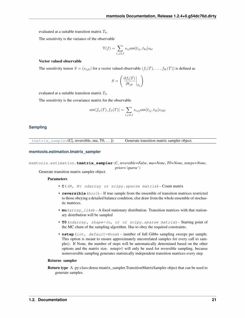
evaluated at a suitable transition matrix 𝑇0.
The sensitivity is the variance of the observable
V(𝑓) =∑𝑖,𝑗,𝑘,𝑙
𝑠𝑖𝑗cov[𝑡𝑖𝑗 , 𝑡𝑘𝑙]𝑠𝑘𝑙
Vector valued observable
The sensitivity tensor 𝑆 = (𝑠𝑖𝑗𝑘) for a vector valued observable (𝑓1(𝑇 ), . . . , 𝑓𝐾(𝑇 )) is defined as
𝑆 =
(𝜕𝑓𝑖(𝑇 )
𝜕𝑡𝑗𝑘
𝑇0
)
evaluated at a suitable transition matrix 𝑇0.
The sensitivity is the covariance matrix for the observable
cov[𝑓𝛼(𝑇 ), 𝑓𝛽(𝑇 )] =∑𝑖,𝑗,𝑘,𝑙
𝑠𝛼𝑖𝑗cov[𝑡𝑖𝑗 , 𝑡𝑘𝑙]𝑠𝛽𝑘𝑙
Sampling
tmatrix_sampler(C[, reversible, mu, T0, . . . ]) Generate transition matrix sampler object.
msmtools.estimation.tmatrix_sampler
msmtools.estimation.tmatrix_sampler(C, reversible=False, mu=None, T0=None, nsteps=None,prior=’sparse’)
Generate transition matrix sampler object.
Parameters
• C ((M, M) ndarray or scipy.sparse matrix) – Count matrix
• reversible (bool) – If true sample from the ensemble of transition matrices restrictedto those obeying a detailed balance condition, else draw from the whole ensemble of stochas-tic matrices.
• mu (array_like) – A fixed stationary distribution. Transition matrices with that station-ary distribution will be sampled
• T0 (ndarray, shape=(n, n) or scipy.sparse matrix) – Starting point ofthe MC chain of the sampling algorithm. Has to obey the required constraints.
• nstep (int, default=None) – number of full Gibbs sampling sweeps per sample.This option is meant to ensure approximately uncorrelated samples for every call to sam-ple(). If None, the number of steps will be automatically determined based on the otheroptions and the matrix size. nstep>1 will only be used for reversible sampling, becausenonreversible sampling generates statistically independent transition matrices every step.
Returns sampler
Return type A :py:class:dense.tmatrix_sampler.TransitionMatrixSampler object that can be used togenerate samples.
1.2. Documentation 21

msmtools Documentation, Release 1.2.4+0.g54dc76d.dirty
Notes
The transition matrix sampler generates transition matrices from the posterior distribution. The posterior distri-bution is given as a product of Dirichlet distributions
P(𝑇 |𝐶) ∝𝑀∏𝑖=1
⎛⎝ 𝑀∏𝑗=1
𝑝𝑐𝑖𝑗𝑖𝑗
⎞⎠The method can generate samples from the posterior under the following constraints
Reversible sampling
Using a MCMC sampler outlined in .. [1] it is ensured that samples from the posterior are reversible, i.e. thereis a probability vector (𝜇𝑖) such that 𝜇𝑖𝑡𝑖𝑗 = 𝜇𝑗𝑡𝑗𝑖 holds for all 𝑖, 𝑗.
Reversible sampling with fixed stationary vector
Using a MCMC sampler outlined in .. [2] it is ensured that samples from the posterior fulfill detailed balancewith respect to a given probability vector (𝜇𝑖).
References
Bootstrap
bootstrap_counts(dtrajs, lagtime[, corrlength]) Generates a randomly resampled count matrix given theinput coordinates.
bootstrap_trajectories(trajs, correla-tion_length)
Generates a randomly resampled trajectory segments.
msmtools.estimation.bootstrap_counts
msmtools.estimation.bootstrap_counts(dtrajs, lagtime, corrlength=None)Generates a randomly resampled count matrix given the input coordinates.
Parameters
• dtrajs (array-like or array-like of array-like) – single or multiplediscrete trajectories. Every trajectory is assumed to be a statistically independent realization.Note that this is often not true and is a weakness with the present bootstrapping approach.
• lagtime (int) – the lag time at which the count matrix will be evaluated
• corrlength (int, optional, default=None) – the correlation length of the dis-crete trajectory. N / corrlength counts will be generated, where N is the total number offrames. If set to None (default), corrlength = lagtime will be used.
Notes
This function can be called multiple times in order to generate randomly resampled realizations of count ma-trices. For each of these realizations you can estimate a transition matrix, and from each of them computingthe observables of your interest. The standard deviation of such a sample of the observable is a model for thestandard error.
22 Chapter 1. Documentation

msmtools Documentation, Release 1.2.4+0.g54dc76d.dirty
The bootstrap will be generated by sampling N/corrlength counts at time tuples (t, t+lagtime), where t is uni-formly sampled over all trajectory time frames in [0,n_i-lagtime]. Here, n_i is the length of trajectory i and N =sum_i n_i is the total number of frames.
See also:
bootstrap_trajectories()
msmtools.estimation.bootstrap_trajectories
msmtools.estimation.bootstrap_trajectories(trajs, correlation_length)Generates a randomly resampled trajectory segments.
Parameters
• trajs (array-like or array-like of array-like) – single or multiple tra-jectories. Every trajectory is assumed to be a statistically independent realization. Note thatthis is often not true and is a weakness with the present bootstrapping approach.
• correlation_length (int) – Correlation length (also known as the or statistical inef-ficiency) of the data. If set to < 1 or > L, where L is the longest trajectory length, the boot-strapping will sample full trajectories. We suggest to select the largest implied timescale orrelaxation timescale as a conservative estimate of the correlation length. If this timescale isunknown, it’s suggested to use full trajectories (set timescale to < 1) or come up with a roughestimate. For computing the error on specific observables, one may use shorter timescales,because the relevant correlation length is the integral of the autocorrelation function of theobservables of interest [3]. The slowest implied timescale is an upper bound for that corre-lation length, and therefore a conservative estimate [4].
Notes
This function can be called multiple times in order to generate randomly resampled trajectory data. In order tocompute error bars on your observable of interest, call this function to generate resampled trajectories, and putthem into your estimator. The standard deviation of such a sample of the observable is a model for the standarderror.
Implements a moving block bootstrapping procedure [1] for generation of randomly resampled count matrixesfrom discrete trajectories. The corrlation length determines the size of trajectory blocks that will remain contigu-ous. For a single trajectory N with correlation length t_corr < N, we will sample floor(N/t_corr) subtrajectoriesof length t_corr using starting time t. t is a uniform random number in [0, N-t_corr-1]. When multiple trajecto-ries are available, N is the total number of timesteps over all trajectories, the algorithm will generate resampleddata with a total number of N (or slightly larger) time steps. Each trajectory of length n_i has a probability of n_ito be selected. Trajectories of length n_i <= t_corr are returned completely. For longer trajectories, segments oflength t_corr are randomly generated.
Note that like all error models for correlated time series data, Bootstrapping just gives you a model for theerror given a number of assumptions [2]. The most critical decisions are: (1) is this approach meaningful at all(only if the trajectories are statistically independent realizations), and (2) select an appropriate timescale of thecorrelation length (see below). Note that transition matrix sampling from the Dirichlet distribution is a muchbetter option from a theoretical point of view, but may also be computationally more demanding.
1.2. Documentation 23

msmtools Documentation, Release 1.2.4+0.g54dc76d.dirty
References
Priors
prior_neighbor(C[, alpha]) Neighbor prior for the given count matrix.prior_const(C[, alpha]) Constant prior for given count matrix.prior_rev(C[, alpha]) Prior counts for sampling of reversible transition matri-
ces.
msmtools.estimation.prior_neighbor
msmtools.estimation.prior_neighbor(C, alpha=0.001)Neighbor prior for the given count matrix.
Parameters
• C ((M, M) ndarray or scipy.sparse matrix) – Count matrix
• alpha (float (optional)) – Value of prior counts
Returns B – Prior count matrix
Return type (M, M) ndarray or scipy.sparse matrix
Notes
The neighbor prior 𝑏𝑖𝑗 is defined as
𝑏𝑖𝑗 =
{𝛼 𝑐𝑖𝑗 + 𝑐𝑗𝑖 > 00 else
Examples
>>> import numpy as np>>> from msmtools.estimation import prior_neighbor
>>> C = np.array([[10, 1, 0], [2, 0, 3], [0, 1, 4]])>>> B = prior_neighbor(C)>>> Barray([[ 0.001, 0.001, 0. ],
[ 0.001, 0. , 0.001],[ 0. , 0.001, 0.001]])
msmtools.estimation.prior_const
msmtools.estimation.prior_const(C, alpha=0.001)Constant prior for given count matrix.
Parameters
• C ((M, M) ndarray or scipy.sparse matrix) – Count matrix
• alpha (float (optional)) – Value of prior counts
24 Chapter 1. Documentation

msmtools Documentation, Release 1.2.4+0.g54dc76d.dirty
Returns B – Prior count matrix
Return type (M, M) ndarray
Notes
The prior is defined as
𝑏𝑖𝑗 = 𝛼 ∀𝑖, 𝑗
Examples
>>> import numpy as np>>> from msmtools.estimation import prior_const
>>> C = np.array([[10, 1, 0], [2, 0, 3], [0, 1, 4]])>>> B = prior_const(C)>>> Barray([[ 0.001, 0.001, 0.001],
[ 0.001, 0.001, 0.001],[ 0.001, 0.001, 0.001]])
msmtools.estimation.prior_rev
msmtools.estimation.prior_rev(C, alpha=-1.0)Prior counts for sampling of reversible transition matrices.
Prior is defined as
b_ij= alpha if i<=j b_ij=0 else
Parameters
• C ((M, M) ndarray or scipy.sparse matrix) – Count matrix
• alpha (float (optional)) – Value of prior counts
Returns B – Matrix of prior counts
Return type (M, M) ndarray
Notes
The reversible prior is a matrix with -1 on the upper triangle. Adding this prior respects the fact that for areversible transition matrix the degrees of freedom correspond essentially to the upper triangular part of thematrix.
The prior is defined as
𝑏𝑖𝑗 =
{𝛼 𝑖 ≤ 𝑗0 elsewhere
1.2. Documentation 25

msmtools Documentation, Release 1.2.4+0.g54dc76d.dirty
Examples
>>> import numpy as np>>> from msmtools.estimation import prior_rev
>>> C = np.array([[10, 1, 0], [2, 0, 3], [0, 1, 4]])>>> B = prior_rev(C)>>> Barray([[-1., -1., -1.],
[ 0., -1., -1.],[ 0., 0., -1.]])
1.2.2 analysis - MSM analysis functions (msmtools.analysis)
This module contains functions to analyze a created Markov model, which is specified with a transition matrix T.
Validation
is_transition_matrix(T[, tol]) Check if the given matrix is a transition matrix.is_tmatrix(T[, tol]) Check if the given matrix is a transition matrix.is_rate_matrix(K[, tol]) Check if the given matrix is a rate matrix.is_connected(T[, directed]) Check connectivity of the given matrix.is_reversible(T[, mu, tol]) Check reversibility of the given transition matrix.
msmtools.analysis.is_transition_matrix
msmtools.analysis.is_transition_matrix(T, tol=1e-12)Check if the given matrix is a transition matrix.
Parameters
• T ((M, M) ndarray or scipy.sparse matrix) – Matrix to check
• tol (float (optional)) – Floating point tolerance to check with
Returns is_transition_matrix – True, if T is a valid transition matrix, False otherwise
Return type bool
Notes
A valid transition matrix 𝑃 = (𝑝𝑖𝑗) has non-negative elements, 𝑝𝑖𝑗 ≥ 0, and elements of each row sum up toone,
∑𝑗 𝑝𝑖𝑗 = 1. Matrices wit this property are also called stochastic matrices.
Examples
>>> import numpy as np>>> from msmtools.analysis import is_transition_matrix
26 Chapter 1. Documentation

msmtools Documentation, Release 1.2.4+0.g54dc76d.dirty
>>> A = np.array([[0.4, 0.5, 0.3], [0.2, 0.4, 0.4], [-1, 1, 1]])>>> is_transition_matrix(A)False
>>> T = np.array([[0.9, 0.1, 0.0], [0.5, 0.0, 0.5], [0.0, 0.1, 0.9]])>>> is_transition_matrix(T)True
msmtools.analysis.is_tmatrix
msmtools.analysis.is_tmatrix(T, tol=1e-12)Check if the given matrix is a transition matrix.
Parameters
• T ((M, M) ndarray or scipy.sparse matrix) – Matrix to check
• tol (float (optional)) – Floating point tolerance to check with
Returns is_transition_matrix – True, if T is a valid transition matrix, False otherwise
Return type bool
Notes
A valid transition matrix 𝑃 = (𝑝𝑖𝑗) has non-negative elements, 𝑝𝑖𝑗 ≥ 0, and elements of each row sum up toone,
∑𝑗 𝑝𝑖𝑗 = 1. Matrices wit this property are also called stochastic matrices.
Examples
>>> import numpy as np>>> from msmtools.analysis import is_transition_matrix
>>> A = np.array([[0.4, 0.5, 0.3], [0.2, 0.4, 0.4], [-1, 1, 1]])>>> is_transition_matrix(A)False
>>> T = np.array([[0.9, 0.1, 0.0], [0.5, 0.0, 0.5], [0.0, 0.1, 0.9]])>>> is_transition_matrix(T)True
msmtools.analysis.is_rate_matrix
msmtools.analysis.is_rate_matrix(K, tol=1e-12)Check if the given matrix is a rate matrix.
Parameters
• K ((M, M) ndarray or scipy.sparse matrix) – Matrix to check
• tol (float (optional)) – Floating point tolerance to check with
Returns is_rate_matrix – True, if K is a valid rate matrix, False otherwise
1.2. Documentation 27

msmtools Documentation, Release 1.2.4+0.g54dc76d.dirty
Return type bool
Notes
A valid rate matrix 𝐾 = (𝑘𝑖𝑗) has non-negative off diagonal elements, 𝑘𝑖𝑗 ≤ 0, for 𝑖 = 𝑗, and elements of eachrow sum up to zero,
∑𝑗 𝑘𝑖𝑗 = 0.
Examples
>>> import numpy as np>>> from msmtools.analysis import is_rate_matrix
>>> A = np.array([[0.5, -0.5, -0.2], [-0.3, 0.6, -0.3], [-0.2, 0.2, 0.0]])>>> is_rate_matrix(A)False
>>> K = np.array([[-0.3, 0.2, 0.1], [0.5, -0.5, 0.0], [0.1, 0.1, -0.2]])>>> is_rate_matrix(K)True
msmtools.analysis.is_connected
msmtools.analysis.is_connected(T, directed=True)Check connectivity of the given matrix.
Parameters
• T ((M, M) ndarray or scipy.sparse matrix) – Matrix to check
• directed (bool (optional)) – If True respect direction of transitions, if False donot distinguish between forward and backward transitions
Returns is_connected – True, if T is connected, False otherwise
Return type bool
Notes
A transition matrix 𝑇 = (𝑡𝑖𝑗) is connected if for any pair of states (𝑖, 𝑗) one can reach state 𝑗 from state 𝑖 in afinite number of steps.
In more precise terms: For any pair of states (𝑖, 𝑗) there exists a number 𝑁 = 𝑁(𝑖, 𝑗), so that the probability ofgoing from state 𝑖 to state 𝑗 in 𝑁 steps is positive, P(𝑋𝑁 = 𝑗|𝑋0 = 𝑖) > 0.
A transition matrix with this property is also called irreducible.
Viewing the transition matrix as the adjency matrix of a (directed) graph the transition matrix is irreducible if andonly if the corresponding graph has a single connected component. Connectivity of a graph can be efficientlychecked using Tarjan’s algorithm.
28 Chapter 1. Documentation

msmtools Documentation, Release 1.2.4+0.g54dc76d.dirty
References
Examples
>>> import numpy as np>>> from msmtools.analysis import is_connected
>>> A = np.array([[0.9, 0.1, 0.0], [0.5, 0.0, 0.5], [0.0, 0.0, 1.0]])>>> is_connected(A)False
>>> T = np.array([[0.9, 0.1, 0.0], [0.5, 0.0, 0.5], [0.0, 0.1, 0.9]])>>> is_connected(T)True
msmtools.analysis.is_reversible
msmtools.analysis.is_reversible(T, mu=None, tol=1e-12)Check reversibility of the given transition matrix.
Parameters
• T ((M, M) ndarray or scipy.sparse matrix) – Transition matrix
• mu ((M,) ndarray (optional)) – Test reversibility with respect to this vector
• tol (float (optional)) – Floating point tolerance to check with
Returns is_reversible – True, if T is reversible, False otherwise
Return type bool
Notes
A transition matrix 𝑇 = (𝑡𝑖𝑗) is reversible with respect to a probability vector 𝜇 = (𝜇𝑖) if the follwing holds,
𝜇𝑖 𝑡𝑖𝑗 = 𝜇𝑗 𝑡𝑗𝑖.
In this case 𝜇 is the stationary vector for 𝑇 , so that 𝜇𝑇𝑇 = 𝜇𝑇 .
If the stationary vector is unknown it is computed from 𝑇 before reversibility is checked.
A reversible transition matrix has purely real eigenvalues. The left eigenvectors (𝑙𝑖) can be computed from righteigenvectors (𝑟𝑖) via 𝑙𝑖 = 𝜇𝑖𝑟𝑖.
Examples
>>> import numpy as np>>> from msmtools.analysis import is_reversible
>>> P = np.array([[0.8, 0.1, 0.1], [0.5, 0.0, 0.5], [0.0, 0.1, 0.9]])>>> is_reversible(P)False
1.2. Documentation 29
msmtools Documentation, Release 1.2.4+0.g54dc76d.dirty
>>> T = np.array([[0.9, 0.1, 0.0], [0.5, 0.0, 0.5], [0.0, 0.1, 0.9]])>>> is_reversible(T)True
Decomposition
Decomposition routines use the scipy LAPACK bindings for dense numpy-arrays and the ARPACK bindings for scipysparse matrices.
stationary_distribution(T) Compute stationary distribution of stochastic matrix T.statdist(T) Compute stationary distribution of stochastic matrix T.eigenvalues(T[, k, ncv, reversible, mu]) Find eigenvalues of the transition matrix.eigenvectors(T[, k, right, ncv, reversible, mu]) Compute eigenvectors of given transition matrix.rdl_decomposition(T[, k, norm, ncv, . . . ]) Compute the decomposition into eigenvalues, left and
right eigenvectors.timescales(T[, tau, k, ncv, reversible, mu]) Compute implied time scales of given transition matrix.
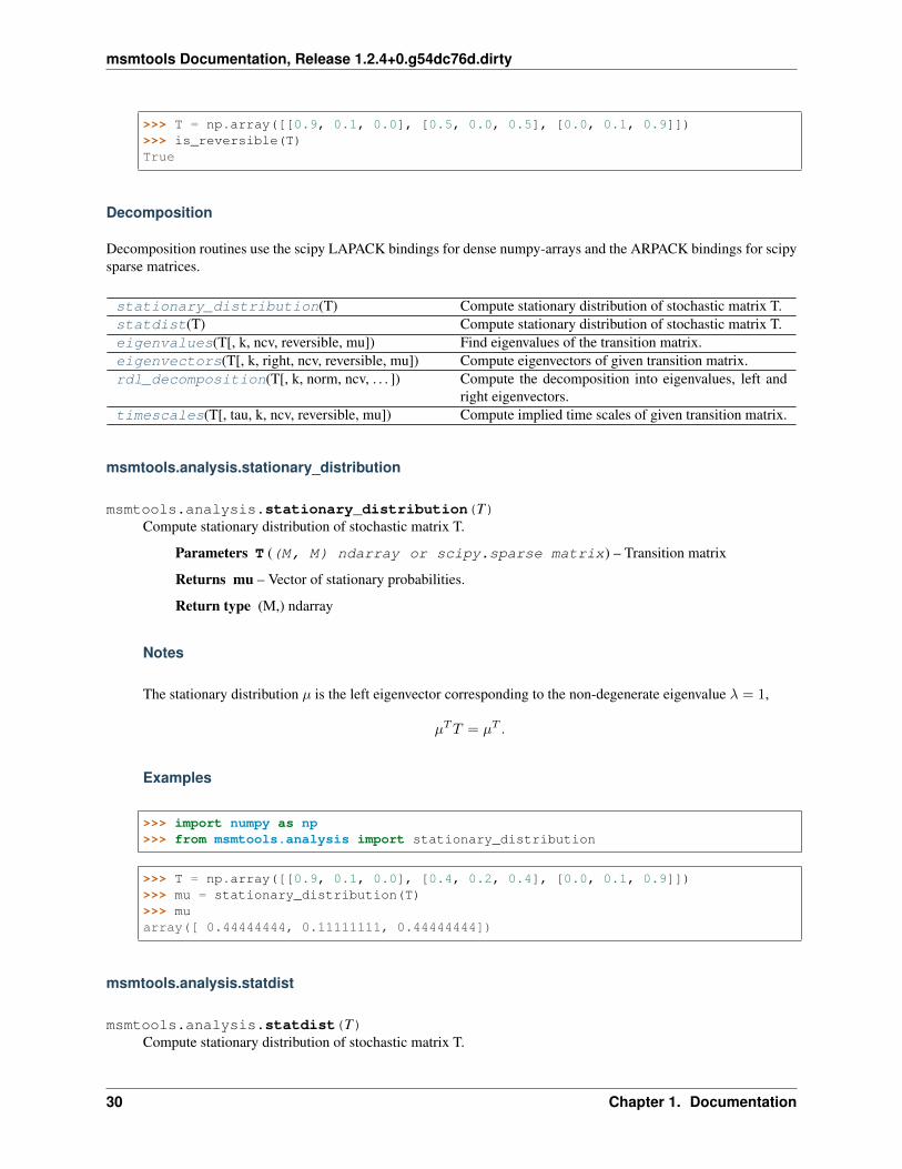
msmtools.analysis.stationary_distribution
msmtools.analysis.stationary_distribution(T)Compute stationary distribution of stochastic matrix T.
Parameters T ((M, M) ndarray or scipy.sparse matrix) – Transition matrix
Returns mu – Vector of stationary probabilities.
Return type (M,) ndarray
Notes
The stationary distribution 𝜇 is the left eigenvector corresponding to the non-degenerate eigenvalue 𝜆 = 1,
𝜇𝑇𝑇 = 𝜇𝑇 .
Examples
>>> import numpy as np>>> from msmtools.analysis import stationary_distribution
>>> T = np.array([[0.9, 0.1, 0.0], [0.4, 0.2, 0.4], [0.0, 0.1, 0.9]])>>> mu = stationary_distribution(T)>>> muarray([ 0.44444444, 0.11111111, 0.44444444])
msmtools.analysis.statdist
msmtools.analysis.statdist(T)Compute stationary distribution of stochastic matrix T.
30 Chapter 1. Documentation

msmtools Documentation, Release 1.2.4+0.g54dc76d.dirty
Parameters T ((M, M) ndarray or scipy.sparse matrix) – Transition matrix
Returns mu – Vector of stationary probabilities.
Return type (M,) ndarray
Notes
The stationary distribution 𝜇 is the left eigenvector corresponding to the non-degenerate eigenvalue 𝜆 = 1,
𝜇𝑇𝑇 = 𝜇𝑇 .
Examples
>>> import numpy as np>>> from msmtools.analysis import stationary_distribution
>>> T = np.array([[0.9, 0.1, 0.0], [0.4, 0.2, 0.4], [0.0, 0.1, 0.9]])>>> mu = stationary_distribution(T)>>> muarray([ 0.44444444, 0.11111111, 0.44444444])
msmtools.analysis.eigenvalues
msmtools.analysis.eigenvalues(T, k=None, ncv=None, reversible=False, mu=None)Find eigenvalues of the transition matrix.
Parameters
• T ((M, M) ndarray or sparse matrix) – Transition matrix
• k (int (optional)) – Compute the first k eigenvalues of T
• ncv (int (optional)) – The number of Lanczos vectors generated, ncv must be greaterthan k; it is recommended that ncv > 2*k
• reversible (bool, optional) – Indicate that transition matrix is reversible
• mu ((M,) ndarray, optional) – Stationary distribution of T
Returns w – Eigenvalues of T. If k is specified, w has shape (k,)
Return type (M,) ndarray
Notes
Eigenvalues are returned in order of decreasing magnitude.
If reversible=True the the eigenvalues of the similar symmetric matrix sqrt(mu_i / mu_j) p_{ij} will be computed.
The precomputed stationary distribution will only be used if reversible=True.
1.2. Documentation 31

msmtools Documentation, Release 1.2.4+0.g54dc76d.dirty
Examples
>>> import numpy as np>>> from msmtools.analysis import eigenvalues
>>> T = np.array([[0.9, 0.1, 0.0], [0.5, 0.0, 0.5], [0.0, 0.1, 0.9]])>>> w = eigenvalues(T)>>> warray([ 1.0+0.j, 0.9+0.j, -0.1+0.j])
msmtools.analysis.eigenvectors
msmtools.analysis.eigenvectors(T, k=None, right=True, ncv=None, reversible=False,mu=None)
Compute eigenvectors of given transition matrix.
Parameters
• T (numpy.ndarray, shape(d,d) or scipy.sparse matrix) – Transitionmatrix (stochastic matrix)
• k (int (optional)) – Compute the first k eigenvectors
• ncv (int (optional)) – The number of Lanczos vectors generated, ncv must be greaterthan k; it is recommended that ncv > 2*k
• right (bool, optional) – If right=True compute right eigenvectors, left eigenvectorsotherwise
• reversible (bool, optional) – Indicate that transition matrix is reversible
• mu ((M,) ndarray, optional) – Stationary distribution of T
Returns eigvec – The eigenvectors of T ordered with decreasing absolute value of the correspondingeigenvalue. If k is None then n=d, if k is int then n=k.
Return type numpy.ndarray, shape=(d, n)
See also:
rdl_decomposition()
Notes
Eigenvectors are computed using the scipy interface to the corresponding LAPACK/ARPACK routines.
If reversible=False, the returned eigenvectors 𝑣𝑖 are normalized such that
⟨𝑣𝑖, 𝑣𝑖⟩ = 1
This is the case for right eigenvectors 𝑟𝑖 as well as for left eigenvectors 𝑙𝑖.
If you desire orthonormal left and right eigenvectors please use the rdl_decomposition method.
If reversible=True the the eigenvectors of the similar symmetric matrix sqrt(mu_i / mu_j) p_{ij} will be used tocompute the eigenvectors of T.
The precomputed stationary distribution will only be used if reversible=True.
32 Chapter 1. Documentation

msmtools Documentation, Release 1.2.4+0.g54dc76d.dirty
Examples
>>> import numpy as np>>> from msmtools.analysis import eigenvectors
>>> T = np.array([[0.9, 0.1, 0.0], [0.5, 0.0, 0.5], [0.0, 0.1, 0.9]])>>> R = eigenvectors(T)
Matrix with right eigenvectors as columns
>>> Rarray([[ 5.77350269e-01, 7.07106781e-01, 9.90147543e-02], ...
msmtools.analysis.rdl_decomposition
msmtools.analysis.rdl_decomposition(T, k=None, norm=’auto’, ncv=None, reversible=False,mu=None)
Compute the decomposition into eigenvalues, left and right eigenvectors.
Parameters
• T ((M, M) ndarray or sparse matrix) – Transition matrix
• k (int (optional)) – Number of eigenvector/eigenvalue pairs
• norm ({'standard', 'reversible', 'auto'}, optional) – which normal-ization convention to use
norm’stan-dard’
LR = Id, is a probabilitydistribution, the stationary distributionof T. Righteigenvectors Rhave a 2-norm of 1
’re-versible’
R and L are related via L[0, :]*R
’auto’ reversible if T is reversible, else standard.
• ncv (int (optional)) – The number of Lanczos vectors generated, ncv must be greaterthan k; it is recommended that ncv > 2*k
• reversible (bool, optional) – Indicate that transition matrix is reversible
• mu ((M,) ndarray, optional) – Stationary distribution of T
Returns
• R ((M, M) ndarray) – The normalized (“unit length”) right eigenvectors, such that thecolumn R[:,i] is the right eigenvector corresponding to the eigenvalue w[i], dot(T,R[:,i])``=``w[i]*R[:,i]
• D ((M, M) ndarray) – A diagonal matrix containing the eigenvalues, each repeated accordingto its multiplicity
• L ((M, M) ndarray) – The normalized (with respect to R) left eigenvectors, such that the rowL[i, :] is the left eigenvector corresponding to the eigenvalue w[i], dot(L[i, :],T)``=``w[i]*L[i, :]
1.2. Documentation 33

msmtools Documentation, Release 1.2.4+0.g54dc76d.dirty
Examples
>>> import numpy as np>>> from msmtools.analysis import rdl_decomposition
>>> T = np.array([[0.9, 0.1, 0.0], [0.5, 0.0, 0.5], [0.0, 0.1, 0.9]])>>> R, D, L = rdl_decomposition(T)
Matrix with right eigenvectors as columns
>>> Rarray([[ 1.00000000e+00, 1.04880885e+00, 3.16227766e-01], ...
Diagonal matrix with eigenvalues
>>> Darray([[ 1.0+0.j, 0.0+0.j, 0.0+0.j],
[ 0.0+0.j, 0.9+0.j, 0.0+0.j],[ 0.0+0.j, 0.0+0.j, -0.1+0.j]])
Matrix with left eigenvectors as rows
>>> L # +doctest: +ELLIPSISarray([[ 4.54545455e-01, 9.09090909e-02, 4.54545455e-01], ...
msmtools.analysis.timescales
msmtools.analysis.timescales(T, tau=1, k=None, ncv=None, reversible=False, mu=None)Compute implied time scales of given transition matrix.
Parameters
• T ((M, M) ndarray or scipy.sparse matrix) – Transition matrix
• tau (int (optional)) – The time-lag (in elementary time steps of the microstate tra-jectory) at which the given transition matrix was constructed.
• k (int (optional)) – Compute the first k implied time scales.
• ncv (int (optional, for sparse T only)) – The number of Lanczos vectorsgenerated, ncv must be greater than k; it is recommended that ncv > 2*k
• reversible (bool, optional) – Indicate that transition matrix is reversible
• mu ((M,) ndarray, optional) – Stationary distribution of T
Returns ts – The implied time scales of the transition matrix. If k is not None then the shape of ts is(k,).
Return type (M,) ndarray
Notes
The implied time scale 𝑡𝑖 is defined as
𝑡𝑖 = − 𝜏
log|𝜆𝑖|
34 Chapter 1. Documentation

msmtools Documentation, Release 1.2.4+0.g54dc76d.dirty
If reversible=True the the eigenvalues of the similar symmetric matrix sqrt(mu_i / mu_j) p_{ij} will be computed.
The precomputed stationary distribution will only be used if reversible=True.
Examples
>>> import numpy as np>>> from msmtools.analysis import timescales
>>> T = np.array([[0.9, 0.1, 0.0], [0.5, 0.0, 0.5], [0.0, 0.1, 0.9]])>>> ts = timescales(T)>>> tsarray([ inf, 9.49122158, 0.43429448])
Expected counts
expected_counts(T, p0, N) Compute expected transition counts for Markov chainwith n steps.
expected_counts_stationary(T, N[, mu]) Expected transition counts for Markov chain in equilib-rium.
msmtools.analysis.expected_counts
msmtools.analysis.expected_counts(T, p0, N)Compute expected transition counts for Markov chain with n steps.
Parameters
• T ((M, M) ndarray or sparse matrix) – Transition matrix
• p0 ((M,) ndarray) – Initial (probability) vector
• N (int) – Number of steps to take
Returns EC – Expected value for transition counts after N steps
Return type (M, M) ndarray or sparse matrix
Notes
Expected counts can be computed via the following expression
E[𝐶(𝑁)] =
𝑁−1∑𝑘=0
diag(𝑝𝑇𝑇 𝑘)𝑇
Examples
>>> import numpy as np>>> from msmtools.analysis import expected_counts
1.2. Documentation 35

msmtools Documentation, Release 1.2.4+0.g54dc76d.dirty
>>> T = np.array([[0.9, 0.1, 0.0], [0.5, 0.0, 0.5], [0.0, 0.1, 0.9]])>>> p0 = np.array([1.0, 0.0, 0.0])>>> N = 100>>> EC = expected_counts(T, p0, N)
>>> ECarray([[ 45.44616147, 5.0495735 , 0. ],
[ 4.50413223, 0. , 4.50413223],[ 0. , 4.04960006, 36.44640052]])
msmtools.analysis.expected_counts_stationary
msmtools.analysis.expected_counts_stationary(T, N, mu=None)Expected transition counts for Markov chain in equilibrium.
Parameters
• T ((M, M) ndarray or sparse matrix) – Transition matrix.
• N (int) – Number of steps for chain.
• mu ((M,) ndarray (optional)) – Stationary distribution for T. If mu is not speci-fied it will be computed from T.
Returns EC – Expected value for transition counts after N steps.
Return type (M, M) ndarray or sparse matrix
Notes
Since 𝜇 is stationary for 𝑇 we have
E[𝐶(𝑁)] = 𝑁𝐷𝜇𝑇.
𝐷𝜇 is a diagonal matrix. Elements on the diagonal are given by the stationary vector 𝜇
Examples
>>> import numpy as np>>> from msmtools.analysis import expected_counts_stationary
>>> T = np.array([[0.9, 0.1, 0.0], [0.5, 0.0, 0.5], [0.0, 0.1, 0.9]])>>> N = 100>>> EC = expected_counts_stationary(T, N)
>>> ECarray([[ 40.90909091, 4.54545455, 0. ],
[ 4.54545455, 0. , 4.54545455],[ 0. , 4.54545455, 40.90909091]])
Passage times
36 Chapter 1. Documentation

msmtools Documentation, Release 1.2.4+0.g54dc76d.dirty
mfpt(T, target[, origin, tau, mu]) Mean first passage times (from a set of starting states -optional) to a set of target states.
msmtools.analysis.mfpt
msmtools.analysis.mfpt(T, target, origin=None, tau=1, mu=None)Mean first passage times (from a set of starting states - optional) to a set of target states.
Parameters
• T (ndarray or scipy.sparse matrix, shape=(n,n)) – Transition matrix.
• target (int or list of int) – Target states for mfpt calculation.
• origin (int or list of int (optional)) – Set of starting states.
• tau (int (optional)) – The time-lag (in elementary time steps of the microstate tra-jectory) at which the given transition matrix was constructed.
• mu ((n,) ndarray (optional)) – The stationary distribution of the transition matrixT.
Returns m_t – Mean first passage time or vector of mean first passage times.
Return type ndarray, shape=(n,) or shape(1,)
Notes
The mean first passage time E𝑥[𝑇𝑌 ] is the expected hitting time of one state 𝑦 in 𝑌 when starting in state 𝑥.
For a fixed target state 𝑦 it is given by
E𝑥[𝑇𝑦] =
{0 𝑥 = 𝑦
1 +∑
𝑧 𝑇𝑥,𝑧E𝑧[𝑇𝑦] 𝑥 = 𝑦
For a set of target states 𝑌 it is given by
E𝑥[𝑇𝑌 ] =
{0 𝑥 ∈ 𝑌
1 +∑
𝑧 𝑇𝑥,𝑧E𝑧[𝑇𝑌 ] 𝑥 /∈ 𝑌
The mean first passage time between sets, E𝑋 [𝑇𝑌 ], is given by
E𝑋 [𝑇𝑌 ] =∑𝑥∈𝑋
𝜇𝑥E𝑥[𝑇𝑌 ]∑𝑧∈𝑋 𝜇𝑧
References
Examples
>>> import numpy as np>>> from msmtools.analysis import mfpt
>>> T = np.array([[0.9, 0.1, 0.0], [0.5, 0.0, 0.5], [0.0, 0.1, 0.9]])>>> m_t = mfpt(T, 0)>>> m_tarray([ 0., 12., 22.])
1.2. Documentation 37

msmtools Documentation, Release 1.2.4+0.g54dc76d.dirty
Committors and PCCA
committor(T, A, B[, forward, mu]) Compute the committor between sets of microstates.pcca(T, m) Compute meta-stable sets using PCCA++ _[1] and re-
turn the membership of all states to these sets.
msmtools.analysis.committor
msmtools.analysis.committor(T, A, B, forward=True, mu=None)Compute the committor between sets of microstates.
The committor assigns to each microstate a probability that being at this state, the set B will be hit next, ratherthan set A (forward committor), or that the set A has been hit previously rather than set B (backward committor).See [1] for a detailed mathematical description. The present implementation uses the equations given in [2].
Parameters
• T ((M, M) ndarray or scipy.sparse matrix) – Transition matrix
• A (array_like) – List of integer state labels for set A
• B (array_like) – List of integer state labels for set B
• forward (bool) – If True compute the forward committor, else compute the backwardcommittor.
Returns q – Vector of comittor probabilities.
Return type (M,) ndarray
Notes
Committor functions are used to characterize microstates in terms of their probability to being visited during areaction/transition between two disjoint regions of state space A, B.
Forward committor
The forward committor 𝑞(+)𝑖 is defined as the probability that the process starting in i will reach B first, rather
than A.
Using the first hitting time of a set 𝑆,
𝑇𝑆 = inf{𝑡 ≥ 0|𝑋𝑡 ∈ 𝑆}
the forward committor 𝑞(+)𝑖 can be fromally defined as
𝑞(+)𝑖 = P𝑖(𝑇𝐴 < 𝑇𝐵).
The forward committor solves to the following boundary value problem∑𝑗 𝐿𝑖𝑗𝑞
(+)𝑗 = 0 𝑖 ∈ 𝑋 ∖ (𝐴 ∪𝐵)
𝑞(+)𝑖 = 0 𝑖 ∈ 𝐴
𝑞(+)𝑖 = 1 𝑖 ∈ 𝐵
𝐿 = 𝑇 − 𝐼 denotes the generator matrix.
Backward committor
38 Chapter 1. Documentation

msmtools Documentation, Release 1.2.4+0.g54dc76d.dirty
The backward committor is defined as the probability that the process starting in 𝑥 came from 𝐴 rather thanfrom 𝐵.
Using the last exit time of a set 𝑆,
𝑡𝑆 = sup{𝑡 ≥ 0|𝑋𝑡 /∈ 𝑆}
the backward committor can be formally defined as
𝑞(−)𝑖 = P𝑖(𝑡𝐴 < 𝑡𝐵).
The backward comittor solves another boundary value problem∑𝑗 𝐾𝑖𝑗𝑞
(−)𝑗 = 0 𝑖 ∈ 𝑋 ∖ (𝐴 ∪𝐵)
𝑞(−)𝑖 = 1 𝑖 ∈ 𝐴
𝑞(−)𝑖 = 0 𝑖 ∈ 𝐵
𝐾 = (𝐷𝜋𝐿)𝑇 denotes the adjoint generator matrix.
References
Examples
>>> import numpy as np>>> from msmtools.analysis import committor>>> T = np.array([[0.89, 0.1, 0.01], [0.5, 0.0, 0.5], [0.0, 0.1, 0.9]])>>> A = [0]>>> B = [2]
>>> u_plus = committor(T, A, B)>>> u_plusarray([ 0. , 0.5, 1. ])
>>> u_minus = committor(T, A, B, forward=False)>>> u_minusarray([ 1. , 0.45454545, 0. ])
msmtools.analysis.pcca
msmtools.analysis.pcca(T, m)Compute meta-stable sets using PCCA++ _[1] and return the membership of all states to these sets.
Parameters
• T ((n, n) ndarray or scipy.sparse matrix) – Transition matrix
• m (int) – Number of metastable sets
Returns clusters – Membership vectors. clusters[i, j] contains the membership of state i tometastable state j
Return type (n, m) ndarray
1.2. Documentation 39

msmtools Documentation, Release 1.2.4+0.g54dc76d.dirty
Notes
Perron cluster center analysis assigns each microstate a vector of membership probabilities. This assignementis performed using the right eigenvectors of the transition matrix. Membership probabilities are computed vianumerical optimization of the entries of a membership matrix.
References
Fingerprints
fingerprint_correlation(T, obs1[, obs2, . . . ]) Dynamical fingerprint for equilibrium correlation ex-periment.
fingerprint_relaxation(T, p0, obs[, tau, k,ncv])
Dynamical fingerprint for relaxation experiment.
expectation(T, a[, mu]) Equilibrium expectation value of a given observable.correlation(T, obs1[, obs2, times, maxtime, . . . ]) Time-correlation for equilibrium experiment.relaxation(T, p0, obs[, times, k, ncv]) Relaxation experiment.
msmtools.analysis.fingerprint_correlation
msmtools.analysis.fingerprint_correlation(T, obs1, obs2=None, tau=1, k=None,ncv=None)
Dynamical fingerprint for equilibrium correlation experiment.
Parameters
• T ((M, M) ndarray or scipy.sparse matrix) – Transition matrix
• obs1 ((M,) ndarray) – Observable, represented as vector on state space
• obs2 ((M,) ndarray (optional)) – Second observable, for cross-correlations
• k (int (optional)) – Number of time-scales and amplitudes to compute
• tau (int (optional)) – Lag time of given transition matrix, for correct time-scales
• ncv (int (optional)) – The number of Lanczos vectors generated, ncv must be greaterthan k; it is recommended that ncv > 2*k
Returns
• timescales ((N,) ndarray) – Time-scales of the transition matrix
• amplitudes ((N,) ndarray) – Amplitudes for the correlation experiment
See also:
correlation(), fingerprint_relaxation()
References
Notes
Fingerprints are a combination of time-scale and amplitude spectrum for a equilibrium correlation or a non-equilibrium relaxation experiment.
40 Chapter 1. Documentation

msmtools Documentation, Release 1.2.4+0.g54dc76d.dirty
Auto-correlation
The auto-correlation of an observable 𝑎(𝑥) for a system in equilibrium is
E𝜇[𝑎(𝑥, 0)𝑎(𝑥, 𝑡)] =∑𝑥
𝜇(𝑥)𝑎(𝑥, 0)𝑎(𝑥, 𝑡)
𝑎(𝑥, 0) = 𝑎(𝑥) is the observable at time 𝑡 = 0. It can be propagated forward in time using the t-step transitionmatrix 𝑝𝑡(𝑥, 𝑦).
The propagated observable at time 𝑡 is 𝑎(𝑥, 𝑡) =∑
𝑦 𝑝𝑡(𝑥, 𝑦)𝑎(𝑦, 0).
Using the eigenvlaues and eigenvectors of the transition matrix the autocorrelation can be written as
E𝜇[𝑎(𝑥, 0)𝑎(𝑥, 𝑡)] =∑𝑖
𝜆𝑡𝑖⟨𝑎, 𝑟𝑖⟩𝜇⟨𝑙𝑖, 𝑎⟩.
The fingerprint amplitudes 𝛾𝑖 are given by
𝛾𝑖 = ⟨𝑎, 𝑟𝑖⟩𝜇⟨𝑙𝑖, 𝑎⟩.
And the fingerprint time scales 𝑡𝑖 are given by
𝑡𝑖 = − 𝜏
log|𝜆𝑖|.
Cross-correlation
The cross-correlation of two observables 𝑎(𝑥), 𝑏(𝑥) is similarly given
E𝜇[𝑎(𝑥, 0)𝑏(𝑥, 𝑡)] =∑𝑥
𝜇(𝑥)𝑎(𝑥, 0)𝑏(𝑥, 𝑡)
The fingerprint amplitudes 𝛾𝑖 are similarly given in terms of the eigenvectors
𝛾𝑖 = ⟨𝑎, 𝑟𝑖⟩𝜇⟨𝑙𝑖, 𝑏⟩.
Examples
>>> import numpy as np>>> from msmtools.analysis import fingerprint_correlation
>>> T = np.array([[0.9, 0.1, 0.0], [0.5, 0.0, 0.5], [0.0, 0.1, 0.9]])>>> a = np.array([1.0, 0.0, 0.0])>>> ts, amp = fingerprint_correlation(T, a)
>>> tsarray([ inf, 9.49122158, 0.43429448])
>>> amparray([ 0.20661157, 0.22727273, 0.02066116])
msmtools.analysis.fingerprint_relaxation
msmtools.analysis.fingerprint_relaxation(T, p0, obs, tau=1, k=None, ncv=None)Dynamical fingerprint for relaxation experiment.
The dynamical fingerprint is given by the implied time-scale spectrum together with the corresponding ampli-tudes.
1.2. Documentation 41

msmtools Documentation, Release 1.2.4+0.g54dc76d.dirty
Parameters
• T ((M, M) ndarray or scipy.sparse matrix) – Transition matrix
• obs1 ((M,) ndarray) – Observable, represented as vector on state space
• obs2 ((M,) ndarray (optional)) – Second observable, for cross-correlations
• k (int (optional)) – Number of time-scales and amplitudes to compute
• tau (int (optional)) – Lag time of given transition matrix, for correct time-scales
• ncv (int (optional)) – The number of Lanczos vectors generated, ncv must be greaterthan k; it is recommended that ncv > 2*k
Returns
• timescales ((N,) ndarray) – Time-scales of the transition matrix
• amplitudes ((N,) ndarray) – Amplitudes for the relaxation experiment
See also:
relaxation(), fingerprint_correlation()
References
Notes
Fingerprints are a combination of time-scale and amplitude spectrum for a equilibrium correlation or a non-equilibrium relaxation experiment.
Relaxation
A relaxation experiment looks at the time dependent expectation value of an observable for a system out ofequilibrium
E𝑤0 [𝑎(𝑥, 𝑡)] =∑𝑥
𝑤0(𝑥)𝑎(𝑥, 𝑡) =∑𝑥
𝑤0(𝑥)∑𝑦
𝑝𝑡(𝑥, 𝑦)𝑎(𝑦).
The fingerprint amplitudes 𝛾𝑖 are given by
𝛾𝑖 = ⟨𝑤0, 𝑟𝑖⟩⟨𝑙𝑖, 𝑎⟩.
And the fingerprint time scales 𝑡𝑖 are given by
𝑡𝑖 = − 𝜏
log|𝜆𝑖|.
Examples
>>> import numpy as np>>> from msmtools.analysis import fingerprint_relaxation
>>> T = np.array([[0.9, 0.1, 0.0], [0.5, 0.0, 0.5], [0.0, 0.1, 0.9]])>>> p0 = np.array([1.0, 0.0, 0.0])>>> a = np.array([1.0, 0.0, 0.0])>>> ts, amp = fingerprint_relaxation(T, p0, a)
42 Chapter 1. Documentation

msmtools Documentation, Release 1.2.4+0.g54dc76d.dirty
>>> tsarray([ inf, 9.49122158, 0.43429448])
>>> amparray([ 0.45454545, 0.5 , 0.04545455])
msmtools.analysis.expectation
msmtools.analysis.expectation(T, a, mu=None)Equilibrium expectation value of a given observable.
Parameters
• T ((M, M) ndarray or scipy.sparse matrix) – Transition matrix
• a ((M,) ndarray) – Observable vector
• mu ((M,) ndarray (optional)) – The stationary distribution of T. If given, the sta-tionary distribution will not be recalculated (saving lots of time)
Returns val – Equilibrium expectation value fo the given observable
Return type float
Notes
The equilibrium expectation value of an observable a is defined as follows
E𝜇[𝑎] =∑𝑖
𝜇𝑖𝑎𝑖
𝜇 = (𝜇𝑖) is the stationary vector of the transition matrix 𝑇 .
Examples
>>> import numpy as np>>> from msmtools.analysis import expectation
>>> T = np.array([[0.9, 0.1, 0.0], [0.5, 0.0, 0.5], [0.0, 0.1, 0.9]])>>> a = np.array([1.0, 0.0, 1.0])>>> m_a = expectation(T, a)>>> m_a0.909090909...
msmtools.analysis.correlation
msmtools.analysis.correlation(T, obs1, obs2=None, times=1, maxtime=None, k=None,ncv=None, return_times=False)
Time-correlation for equilibrium experiment.
Parameters
• T ((M, M) ndarray or scipy.sparse matrix) – Transition matrix
1.2. Documentation 43

msmtools Documentation, Release 1.2.4+0.g54dc76d.dirty
• obs1 ((M,) ndarray) – Observable, represented as vector on state space
• obs2 ((M,) ndarray (optional)) – Second observable, for cross-correlations
• times (array-like of int (optional), default=(1)) – List of times (intau) at which to compute correlation
• maxtime (int, optional, default=None) – Maximum time step to use. Equiv-alent to . Alternative to times.
• k (int (optional)) – Number of eigenvalues and eigenvectors to use for computation
• ncv (int (optional)) – The number of Lanczos vectors generated, ncv must be greaterthan k; it is recommended that ncv > 2*k
Returns
• correlations (ndarray) – Correlation values at given times
• times (ndarray, optional) – time points at which the correlation was computed (if re-turn_times=True)
References
Notes
Auto-correlation
The auto-correlation of an observable 𝑎(𝑥) for a system in equilibrium is
E𝜇[𝑎(𝑥, 0)𝑎(𝑥, 𝑡)] =∑𝑥
𝜇(𝑥)𝑎(𝑥, 0)𝑎(𝑥, 𝑡)
𝑎(𝑥, 0) = 𝑎(𝑥) is the observable at time 𝑡 = 0. It can be propagated forward in time using the t-step transitionmatrix 𝑝𝑡(𝑥, 𝑦).
The propagated observable at time 𝑡 is 𝑎(𝑥, 𝑡) =∑
𝑦 𝑝𝑡(𝑥, 𝑦)𝑎(𝑦, 0).
Using the eigenvlaues and eigenvectors of the transition matrix the autocorrelation can be written as
E𝜇[𝑎(𝑥, 0)𝑎(𝑥, 𝑡)] =∑𝑖
𝜆𝑡𝑖⟨𝑎, 𝑟𝑖⟩𝜇⟨𝑙𝑖, 𝑎⟩.
Cross-correlation
The cross-correlation of two observables 𝑎(𝑥), 𝑏(𝑥) is similarly given
E𝜇[𝑎(𝑥, 0)𝑏(𝑥, 𝑡)] =∑𝑥
𝜇(𝑥)𝑎(𝑥, 0)𝑏(𝑥, 𝑡)
Examples
>>> import numpy as np>>> from msmtools.analysis import correlation
>>> T = np.array([[0.9, 0.1, 0.0], [0.5, 0.0, 0.5], [0.0, 0.1, 0.9]])>>> a = np.array([1.0, 0.0, 0.0])>>> times = np.array([1, 5, 10, 20])
44 Chapter 1. Documentation

msmtools Documentation, Release 1.2.4+0.g54dc76d.dirty
>>> corr = correlation(T, a, times=times)>>> corrarray([ 0.40909091, 0.34081364, 0.28585667, 0.23424263])
msmtools.analysis.relaxation
msmtools.analysis.relaxation(T, p0, obs, times=1, k=None, ncv=None)Relaxation experiment.
The relaxation experiment describes the time-evolution of an expectation value starting in a non-equilibriumsituation.
Parameters
• T ((M, M) ndarray or scipy.sparse matrix) – Transition matrix
• p0 ((M,) ndarray (optional)) – Initial distribution for a relaxation experiment
• obs ((M,) ndarray) – Observable, represented as vector on state space
• times (list of int (optional)) – List of times at which to compute expectation
• k (int (optional)) – Number of eigenvalues and eigenvectors to use for computation
• ncv (int (optional)) – The number of Lanczos vectors generated, ncv must be greaterthan k; it is recommended that ncv > 2*k
Returns res – Array of expectation value at given times
Return type ndarray
References
Notes
Relaxation
A relaxation experiment looks at the time dependent expectation value of an observable for a system out ofequilibrium
E𝑤0[𝑎(𝑥, 𝑡)] =
∑𝑥
𝑤0(𝑥)𝑎(𝑥, 𝑡) =∑𝑥
𝑤0(𝑥)∑𝑦
𝑝𝑡(𝑥, 𝑦)𝑎(𝑦).
Examples
>>> import numpy as np>>> from msmtools.analysis import relaxation
>>> T = np.array([[0.9, 0.1, 0.0], [0.5, 0.0, 0.5], [0.0, 0.1, 0.9]])>>> p0 = np.array([1.0, 0.0, 0.0])>>> a = np.array([1.0, 1.0, 0.0])>>> times = np.array([1, 5, 10, 20])
1.2. Documentation 45

msmtools Documentation, Release 1.2.4+0.g54dc76d.dirty
>>> rel = relaxation(T, p0, a, times=times)>>> relarray([ 1. , 0.8407 , 0.71979377, 0.60624287])
Sensitivity analysis
stationary_distribution_sensitivity(T,j)
Sensitivity matrix of a stationary distribution element.
eigenvalue_sensitivity(T, k) Sensitivity matrix of a specified eigenvalue.timescale_sensitivity(T, k) Sensitivity matrix of a specified time-scale.eigenvector_sensitivity(T, k, j[, right]) Sensitivity matrix of a selected eigenvector element.mfpt_sensitivity(T, target, i) Sensitivity matrix of the mean first-passage time from
specified state.committor_sensitivity(T, A, B, i[, forward]) Sensitivity matrix of a specified committor entry.expectation_sensitivity(T, a) Sensitivity of expectation value of observable A=(a_i).
msmtools.analysis.stationary_distribution_sensitivity
msmtools.analysis.stationary_distribution_sensitivity(T, j)Sensitivity matrix of a stationary distribution element.
Parameters
• T ((M, M) ndarray) – Transition matrix (stochastic matrix).
• j (int) – Index of stationary distribution element for which sensitivity matrix is computed.
Returns S – Sensitivity matrix for the specified element of the stationary distribution.
Return type (M, M) ndarray
msmtools.analysis.eigenvalue_sensitivity
msmtools.analysis.eigenvalue_sensitivity(T, k)Sensitivity matrix of a specified eigenvalue.
Parameters
• T ((M, M) ndarray) – Transition matrix
• k (int) – Compute sensitivity matrix for k-th eigenvalue
Returns S – Sensitivity matrix for k-th eigenvalue.
Return type (M, M) ndarray
msmtools.analysis.timescale_sensitivity
msmtools.analysis.timescale_sensitivity(T, k)Sensitivity matrix of a specified time-scale.
Parameters
• T ((M, M) ndarray) – Transition matrix
46 Chapter 1. Documentation

msmtools Documentation, Release 1.2.4+0.g54dc76d.dirty
• k (int) – Compute sensitivity matrix for the k-th time-scale.
Returns S – Sensitivity matrix for the k-th time-scale.
Return type (M, M) ndarray
msmtools.analysis.eigenvector_sensitivity
msmtools.analysis.eigenvector_sensitivity(T, k, j, right=True)Sensitivity matrix of a selected eigenvector element.
Parameters
• T ((M, M) ndarray) – Transition matrix (stochastic matrix).
• k (int) – Eigenvector index
• j (int) – Element index
• right (bool) – If True compute for right eigenvector, otherwise compute for left eigen-vector.
Returns S – Sensitivity matrix for the j-th element of the k-th eigenvector.
Return type (M, M) ndarray
msmtools.analysis.mfpt_sensitivity
msmtools.analysis.mfpt_sensitivity(T, target, i)Sensitivity matrix of the mean first-passage time from specified state.
Parameters
• T ((M, M) ndarray) – Transition matrix
• target (int or list) – Target state or set for mfpt computation
• i (int) – Compute the sensitivity for state i
Returns S – Sensitivity matrix for specified state
Return type (M, M) ndarray
msmtools.analysis.committor_sensitivity
msmtools.analysis.committor_sensitivity(T, A, B, i, forward=True)Sensitivity matrix of a specified committor entry.
Parameters
• T ((M, M) ndarray) – Transition matrix
• A (array_like) – List of integer state labels for set A
• B (array_like) – List of integer state labels for set B
• i (int) – Compute the sensitivity for committor entry i
• forward (bool (optional)) – Compute the forward committor. If forward is Falsecompute the backward committor.
Returns S – Sensitivity matrix of the specified committor entry.
1.2. Documentation 47

msmtools Documentation, Release 1.2.4+0.g54dc76d.dirty
Return type (M, M) ndarray
msmtools.analysis.expectation_sensitivity
msmtools.analysis.expectation_sensitivity(T, a)Sensitivity of expectation value of observable A=(a_i).
Parameters
• T ((M, M) ndarray) – Transition matrix
• a ((M,) ndarray) – Observable, a[i] is the value of the observable at state i.
Returns S – Sensitivity matrix of the expectation value.
Return type (M, M) ndarray
1.2.3 flux - Reactive flux an transition pathways (msmtools.flux)
This module contains functions to compute reactive flux networks and find dominant reaction pathways in such net-works.
TPT-object
tpt(T, A, B[, mu, qminus, qplus, rate_matrix]) Computes the A->B reactive flux using transition paththeory (TPT)
ReactiveFlux(A, B, flux[, mu, qminus, . . . ]) A->B reactive flux from transition path theory (TPT)
msmtools.flux.tpt
msmtools.flux.tpt(T, A, B, mu=None, qminus=None, qplus=None, rate_matrix=False)Computes the A->B reactive flux using transition path theory (TPT)
Parameters
• T ((M, M) ndarray or scipy.sparse matrix) – Transition matrix (default) orRate matrix (if rate_matrix=True)
• A (array_like) – List of integer state labels for set A
• B (array_like) – List of integer state labels for set B
• mu ((M,) ndarray (optional)) – Stationary vector
• qminus ((M,) ndarray (optional)) – Backward committor for A->B reaction
• qplus ((M,) ndarray (optional)) – Forward committor for A-> B reaction
• = False (rate_matrix) – By default (False), T is a transition matrix. If set to True, Tis a rate matrix.
Returns tpt – A python object containing the reactive A->B flux network and several additionalquantities, such as stationary probability, committors and set definitions.
Return type msmtools.flux.ReactiveFlux object
48 Chapter 1. Documentation

msmtools Documentation, Release 1.2.4+0.g54dc76d.dirty
Notes
The central object used in transition path theory is the forward and backward comittor function.
TPT (originally introduced in [1]) for continous systems has a discrete version outlined in [2]. Here, we use thetransition matrix formulation described in [3].
See also:
msmtools.analysis.committor(), ReactiveFlux()
References
msmtools.flux.ReactiveFlux
class msmtools.flux.ReactiveFlux(A, B, flux, mu=None, qminus=None, qplus=None,gross_flux=None)
A->B reactive flux from transition path theory (TPT)
This object describes a reactive flux, i.e. a network of fluxes from a set of source states A, to a set of sink statesB, via a set of intermediate nodes. Every node has three properties: the stationary probability mu, the forwardcommittor qplus and the backward committor qminus. Every pair of edges has the following properties: a flux,generally a net flux that has no unnecessary back-fluxes, and optionally a gross flux.
Flux objects can be used to compute transition pathways (and their weights) from A to B, the total flux, the totaltransition rate or mean first passage time, and they can be coarse-grained onto a set discretization of the nodeset.
Fluxes can be computed in EMMA using transition path theory - see msmtools.tpt()
Parameters
• A (array_like) – List of integer state labels for set A
• B (array_like) – List of integer state labels for set B
• flux ((n,n) ndarray or scipy sparse matrix) – effective or net flux of A->B pathways
• mu ((n,) ndarray (optional)) – Stationary vector
• qminus ((n,) ndarray (optional)) – Backward committor for A->B reaction
• qplus ((n,) ndarray (optional)) – Forward committor for A-> B reaction
• gross_flux ((n,n) ndarray or scipy sparse matrix) – gross flux of A->B pathways, if available
Notes
Reactive flux contains a flux network from educt states (A) to product states (B).
See also:
msmtools.tpt
__init__(A, B, flux, mu=None, qminus=None, qplus=None, gross_flux=None)x.__init__(. . . ) initializes x; see help(type(x)) for signature
1.2. Documentation 49

msmtools Documentation, Release 1.2.4+0.g54dc76d.dirty
Methods
__init__(A, B, flux[, mu, qminus, qplus, . . . ]) x.__init__(. . . ) initializes x; see help(type(x)) forsignature
coarse_grain(user_sets) Coarse-grains the flux onto user-defined sets.major_flux([fraction]) Returns the main pathway part of the net flux com-
prising at most the requested fraction of the full flux.pathways([fraction, maxiter]) Decompose flux network into dominant reaction
paths.
Attributes
A Returns the set of reactant (source) states.B Returns the set of product (target) statesI Returns the set of intermediate statesbackward_committor Returns the backward committor probabilitycommittor Returns the forward committor probabilityflux Returns the effective or net fluxforward_committor Returns the forward committor probabilitygross_flux Returns the gross A–>B fluxmfpt Returns the rate (inverse mfpt) of A–>B transitionsnet_flux Returns the effective or net fluxnstates Returns the number of states.rate Returns the rate (inverse mfpt) of A–>B transitionsstationary_distribution Returns the stationary distributiontotal_flux Returns the total flux
AReturns the set of reactant (source) states.
BReturns the set of product (target) states
IReturns the set of intermediate states
backward_committorReturns the backward committor probability
coarse_grain(user_sets)Coarse-grains the flux onto user-defined sets.
Parameters user_sets (list of int-iterables) – sets of states that shall be distin-guished in the coarse-grained flux.
Returns (sets, tpt) – sets contains the sets tpt is computed on. The tpt states of the new tptobject correspond to these sets of states in this order. Sets might be identical, if the userhas already provided a complete partition that respects the boundary between A, B and theintermediates. If not, Sets will have more members than provided by the user, containingthe “remainder” states and reflecting the splitting at the A and B boundaries. tpt containsa new tpt object for the coarse-grained flux. All its quantities (gross_flux, net_flux, A, B,committor, backward_committor) are coarse-grained to sets.
Return type (list of int-iterables, tpt-object)
50 Chapter 1. Documentation

msmtools Documentation, Release 1.2.4+0.g54dc76d.dirty
Notes
All user-specified sets will be split (if necessary) to preserve the boundary between A, B and the interme-diate states.
committorReturns the forward committor probability
fluxReturns the effective or net flux
forward_committorReturns the forward committor probability
gross_fluxReturns the gross A–>B flux
major_flux(fraction=0.9)Returns the main pathway part of the net flux comprising at most the requested fraction of the full flux.
mfptReturns the rate (inverse mfpt) of A–>B transitions
net_fluxReturns the effective or net flux
nstatesReturns the number of states.
pathways(fraction=1.0, maxiter=1000)Decompose flux network into dominant reaction paths.
Parameters
• fraction (float, optional) – Fraction of total flux to assemble in pathway de-composition
• maxiter (int, optional) – Maximum number of pathways for decomposition
Returns
• paths (list) – List of dominant reaction pathways
• capacities (list) – List of capacities corresponding to each reactions pathway in paths
References
rateReturns the rate (inverse mfpt) of A–>B transitions
stationary_distributionReturns the stationary distribution
total_fluxReturns the total flux
Reactive flux
1.2. Documentation 51

msmtools Documentation, Release 1.2.4+0.g54dc76d.dirty
flux_matrix(T, pi, qminus, qplus[, netflux]) Compute the TPT flux network for the reaction A–>B.to_netflux(flux) Compute the netflux from the gross flux.flux_production(F) Returns the net flux production for all statesflux_producers(F[, rtol, atol]) Return indexes of states that are net flux producers.flux_consumers(F[, rtol, atol]) Return indexes of states that are net flux producers.coarsegrain(F, sets) Coarse-grains the flux to the given sets.
msmtools.flux.flux_matrix
msmtools.flux.flux_matrix(T, pi, qminus, qplus, netflux=True)Compute the TPT flux network for the reaction A–>B.
Parameters
• T ((M, M) ndarray) – transition matrix
• pi ((M,) ndarray) – Stationary distribution corresponding to T
• qminus ((M,) ndarray) – Backward comittor
• qplus ((M,) ndarray) – Forward committor
• netflux (boolean) – True: net flux matrix will be computed False: gross flux matrixwill be computed
Returns flux – Matrix of flux values between pairs of states.
Return type (M, M) ndarray
Notes
Computation of the flux network relies on transition path theory (TPT) [1]. Here we use discrete transition paththeory [2] in the transition matrix formulation [3].
See also:
committor.forward_committor(), committor.backward_committor()
Notes
Computation of the flux network relies on transition path theory (TPT). The central object used in transitionpath theory is the forward and backward comittor function.
The TPT (gross) flux is defined as
𝑓𝑖𝑗 =
{𝜋𝑖𝑞
(−)𝑖 𝑝𝑖𝑗𝑞
(+)𝑗 𝑖 = 𝑗
0 𝑖 = 𝑗
The TPT net flux is then defined as
𝑓𝑖𝑗 = max{𝑓𝑖𝑗 − 𝑓𝑗𝑖, 0} ∀𝑖, 𝑗.
52 Chapter 1. Documentation

msmtools Documentation, Release 1.2.4+0.g54dc76d.dirty
References
msmtools.flux.to_netflux
msmtools.flux.to_netflux(flux)Compute the netflux from the gross flux.
Parameters flux ((M, M) ndarray) – Matrix of flux values between pairs of states.
Returns netflux – Matrix of netflux values between pairs of states.
Return type (M, M) ndarray
Notes
The netflux or effective current is defined as
𝑓+𝑖𝑗 = max{𝑓𝑖𝑗 − 𝑓𝑗𝑖, 0}
𝑓𝑖𝑗 is the flux for the transition from 𝐴 to 𝐵.
References
msmtools.flux.flux_production
msmtools.flux.flux_production(F)Returns the net flux production for all states
Parameters F ((M, M) ndarray) – Matrix of flux values between pairs of states.
Returns prod – Array containing flux production (positive) or consumption (negative) at each state
Return type (M,) ndarray
msmtools.flux.flux_producers
msmtools.flux.flux_producers(F, rtol=1e-05, atol=1e-12)Return indexes of states that are net flux producers.
Parameters
• F ((M, M) ndarray) – Matrix of flux values between pairs of states.
• rtol (float) – relative tolerance. fulfilled if max(outflux-influx, 0) / max(outflux,influx)< rtol
• atol (float) – absolute tolerance. fulfilled if max(outflux-influx, 0) < atol
Returns producers – indexes of states that are net flux producers. May include “dirty” producers,i.e. states that have influx but still produce more outflux and thereby violate flux conservation.
Return type (M, ) ndarray of int
1.2. Documentation 53

msmtools Documentation, Release 1.2.4+0.g54dc76d.dirty
msmtools.flux.flux_consumers
msmtools.flux.flux_consumers(F, rtol=1e-05, atol=1e-12)Return indexes of states that are net flux producers.
Parameters
• F ((M, M) ndarray) – Matrix of flux values between pairs of states.
• rtol (float) – relative tolerance. fulfilled if max(outflux-influx, 0) / max(outflux,influx)< rtol
• atol (float) – absolute tolerance. fulfilled if max(outflux-influx, 0) < atol
Returns producers – indexes of states that are net flux producers. May include “dirty” producers,i.e. states that have influx but still produce more outflux and thereby violate flux conservation.
Return type (M, ) ndarray of int
msmtools.flux.coarsegrain
msmtools.flux.coarsegrain(F, sets)Coarse-grains the flux to the given sets.
Parameters
• F ((n, n) ndarray or scipy.sparse matrix) – Matrix of flux values betweenpairs of states.
• sets (list of array-like of ints) – The sets of states onto which the flux iscoarse-grained.
Notes
The coarse grained flux is defined as
𝑓𝑐𝐼,𝐽 =∑
𝑖∈𝐼,𝑗∈𝐽
𝑓𝑖,𝑗
Note that if you coarse-grain a net flux, it does n ot necessarily have a net flux property anymore. If want tomake sure you get a netflux, use to_netflux(coarsegrain(F,sets)).
References
Reaction rates and fluxes
total_flux(F[, A]) Compute the total flux, or turnover flux, that is producedby
rate(totflux, pi, qminus) Transition rate for reaction A to B.mfpt(totflux, pi, qminus) Mean first passage time for reaction A to B.
msmtools.flux.total_flux
msmtools.flux.total_flux(F, A=None)
54 Chapter 1. Documentation

msmtools Documentation, Release 1.2.4+0.g54dc76d.dirty
Compute the total flux, or turnover flux, that is produced by the flux sources and consumed by the fluxsinks.
Parameters
• F ((M, M) ndarray) – Matrix of flux values between pairs of states.
• A (array_like (optional)) – List of integer state labels for set A (reactant)
Returns F – The total flux, or turnover flux, that is produced by the flux sources and consumed bythe flux sinks
Return type float
References
msmtools.flux.rate
msmtools.flux.rate(totflux, pi, qminus)Transition rate for reaction A to B.
Parameters
• totflux (float) – The total flux between reactant and product
• pi ((M,) ndarray) – Stationary distribution
• qminus ((M,) ndarray) – Backward comittor
Returns kAB – The reaction rate (per time step of the Markov chain)
Return type float
See also:
committor(), total_flux(), flux_matrix()
Notes
Computation of the rate relies on discrete transition path theory (TPT). The transition rate, i.e. the total numberof reaction events per time step, is given in [1] as:
𝑘𝐴𝐵 =1
𝐹
∑𝑖
𝜋𝑖𝑞(−)𝑖
𝐹 is the total flux for the transition from 𝐴 to 𝐵.
References
msmtools.flux.mfpt
msmtools.flux.mfpt(totflux, pi, qminus)Mean first passage time for reaction A to B.
Parameters
• totflux (float) – The total flux between reactant and product
1.2. Documentation 55

msmtools Documentation, Release 1.2.4+0.g54dc76d.dirty
• pi ((M,) ndarray) – Stationary distribution
• qminus ((M,) ndarray) – Backward comittor
Returns tAB – The mean first-passage time for the A to B reaction
Return type float
See also:
rate()
Notes
Equal to the inverse rate, see [1].
References
Pathway decomposition
pathways(F, A, B[, fraction, maxiter]) Decompose flux network into dominant reaction paths.
msmtools.flux.pathways
msmtools.flux.pathways(F, A, B, fraction=1.0, maxiter=1000)Decompose flux network into dominant reaction paths.
Parameters
• F ((M, M) scipy.sparse matrix) – The flux network (matrix of netflux values)
• A (array_like) – The set of starting states
• B (array_like) – The set of end states
• fraction (float, optional) – Fraction of total flux to assemble in pathway decom-position
• maxiter (int, optional) – Maximum number of pathways for decomposition
Returns
• paths (list) – List of dominant reaction pathways
• capacities (list) – List of capacities corresponding to each reactions pathway in paths
Notes
The default value for fraction is 1.0, i.e. all dominant reaction pathways for the flux network are computed.For large netorks the number of possible reaction paths can increase rapidly so that it becomes prohibitevelyexpensive to compute all possible reaction paths. To prevent this from happening maxiter sets the maximumnumber of reaction pathways that will be computed.
For large flux networks it might be necessary to decrease fraction or to increase maxiter. It is advisable tobegin with a small value for fraction and monitor the number of pathways returned when increasing the value offraction.
56 Chapter 1. Documentation

msmtools Documentation, Release 1.2.4+0.g54dc76d.dirty
References
1.2.4 dtraj - Discrete trajectories functions (msmtools.dtraj)
Discrete trajectory io
read_discrete_trajectory(filename) Read discrete trajectory from ascii file.read_dtraj(filename) Read discrete trajectory from ascii file.write_discrete_trajectory(filename, dtraj) Write discrete trajectory to ascii file.write_dtraj(filename, dtraj) Write discrete trajectory to ascii file.load_discrete_trajectory(filename) Read discrete trajectory form binary file.load_dtraj(filename) Read discrete trajectory form binary file.save_discrete_trajectory(filename, dtraj) Write discrete trajectory to binary file.save_dtraj(filename, dtraj) Write discrete trajectory to binary file.
msmtools.dtraj.read_discrete_trajectory
msmtools.dtraj.read_discrete_trajectory(filename)Read discrete trajectory from ascii file.
Parameters filename (str) – The filename of the discretized trajectory file. The filename caneither contain the full or the relative path to the file.
Returns dtraj – Discrete state trajectory.
Return type (M, ) ndarray of int
See also:
write_discrete_trajectory()
Notes
The discrete trajectory file contains a single column with integer entries.
Examples
>>> import numpy as np>>> import os>>> from tempfile import mktemp>>> from msmtools.dtraj import write_discrete_trajectory, read_discrete_trajectory
Use temporary file
>>> tmpfile = mktemp(suffix=".dtraj")
Discrete trajectory
>>> dtraj = np.array([0, 1, 0, 0, 1, 1, 0])
Write to disk (as ascii file)
1.2. Documentation 57
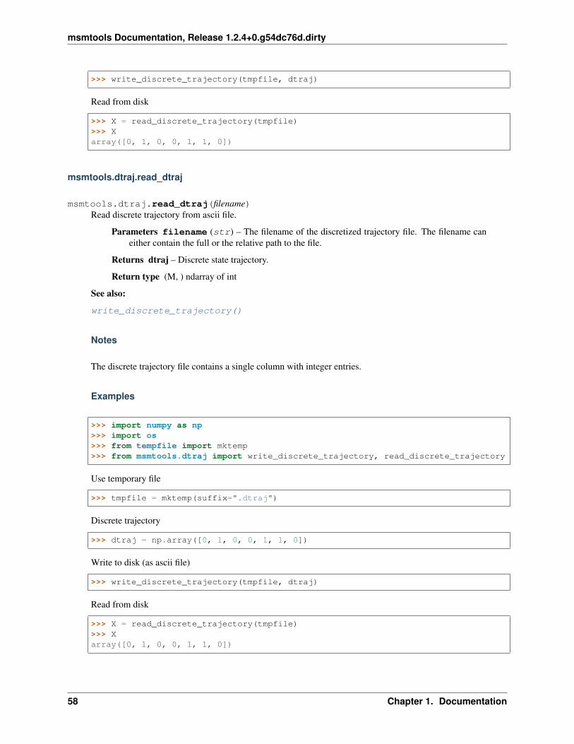
msmtools Documentation, Release 1.2.4+0.g54dc76d.dirty
>>> write_discrete_trajectory(tmpfile, dtraj)
Read from disk
>>> X = read_discrete_trajectory(tmpfile)>>> Xarray([0, 1, 0, 0, 1, 1, 0])
msmtools.dtraj.read_dtraj
msmtools.dtraj.read_dtraj(filename)Read discrete trajectory from ascii file.
Parameters filename (str) – The filename of the discretized trajectory file. The filename caneither contain the full or the relative path to the file.
Returns dtraj – Discrete state trajectory.
Return type (M, ) ndarray of int
See also:
write_discrete_trajectory()
Notes
The discrete trajectory file contains a single column with integer entries.
Examples
>>> import numpy as np>>> import os>>> from tempfile import mktemp>>> from msmtools.dtraj import write_discrete_trajectory, read_discrete_trajectory
Use temporary file
>>> tmpfile = mktemp(suffix=".dtraj")
Discrete trajectory
>>> dtraj = np.array([0, 1, 0, 0, 1, 1, 0])
Write to disk (as ascii file)
>>> write_discrete_trajectory(tmpfile, dtraj)
Read from disk
>>> X = read_discrete_trajectory(tmpfile)>>> Xarray([0, 1, 0, 0, 1, 1, 0])
58 Chapter 1. Documentation

msmtools Documentation, Release 1.2.4+0.g54dc76d.dirty
msmtools.dtraj.write_discrete_trajectory
msmtools.dtraj.write_discrete_trajectory(filename, dtraj)Write discrete trajectory to ascii file.
Parameters
• filename (str) – The filename of the discrete state trajectory file. The filename caneither contain the full or the relative path to the file.
• dtraj (array-like of int) – Discrete state trajectory
See also:
read_discrete_trajectory()
Notes
The discrete trajectory is written to a single column ascii file with integer entries.
Examples
>>> import numpy as np>>> import os>>> from tempfile import mktemp>>> from msmtools.dtraj import write_discrete_trajectory, read_discrete_trajectory
Use temporary file
>>> tmpfile = mktemp()
Discrete trajectory
>>> dtraj = np.array([0, 1, 0, 0, 1, 1, 0])
Write to disk (as ascii file)
>>> write_discrete_trajectory(tmpfile, dtraj)
Read from disk
>>> X = read_discrete_trajectory(tmpfile)>>> Xarray([0, 1, 0, 0, 1, 1, 0])
msmtools.dtraj.write_dtraj
msmtools.dtraj.write_dtraj(filename, dtraj)Write discrete trajectory to ascii file.
Parameters
• filename (str) – The filename of the discrete state trajectory file. The filename caneither contain the full or the relative path to the file.
1.2. Documentation 59

msmtools Documentation, Release 1.2.4+0.g54dc76d.dirty
• dtraj (array-like of int) – Discrete state trajectory
See also:
read_discrete_trajectory()
Notes
The discrete trajectory is written to a single column ascii file with integer entries.
Examples
>>> import numpy as np>>> import os>>> from tempfile import mktemp>>> from msmtools.dtraj import write_discrete_trajectory, read_discrete_trajectory
Use temporary file
>>> tmpfile = mktemp()
Discrete trajectory
>>> dtraj = np.array([0, 1, 0, 0, 1, 1, 0])
Write to disk (as ascii file)
>>> write_discrete_trajectory(tmpfile, dtraj)
Read from disk
>>> X = read_discrete_trajectory(tmpfile)>>> Xarray([0, 1, 0, 0, 1, 1, 0])
msmtools.dtraj.load_discrete_trajectory
msmtools.dtraj.load_discrete_trajectory(filename)Read discrete trajectory form binary file.
Parameters filename (str) – The filename of the discrete state trajectory file. The filename caneither contain the full or the relative path to the file.
Returns dtraj – Discrete state trajectory
Return type (M,) ndarray of int
See also:
save_discrete_trajectory()
Notes
The binary file is a one dimensional numpy array of integers stored in numpy .npy format.
60 Chapter 1. Documentation

msmtools Documentation, Release 1.2.4+0.g54dc76d.dirty
Examples
>>> import numpy as np>>> import os>>> from tempfile import mktemp>>> from msmtools.dtraj import load_discrete_trajectory, save_discrete_trajectory
Use temporary file
>>> tmpfile = mktemp(suffix='.npy')
Discrete trajectory
>>> dtraj = np.array([0, 1, 0, 0, 1, 1, 0])
Write to disk (as npy file)
>>> save_discrete_trajectory(tmpfile, dtraj)
Read from disk
>>> X = load_discrete_trajectory(tmpfile)>>> Xarray([0, 1, 0, 0, 1, 1, 0])
msmtools.dtraj.load_dtraj
msmtools.dtraj.load_dtraj(filename)Read discrete trajectory form binary file.
Parameters filename (str) – The filename of the discrete state trajectory file. The filename caneither contain the full or the relative path to the file.
Returns dtraj – Discrete state trajectory
Return type (M,) ndarray of int
See also:
save_discrete_trajectory()
Notes
The binary file is a one dimensional numpy array of integers stored in numpy .npy format.
Examples
>>> import numpy as np>>> import os>>> from tempfile import mktemp>>> from msmtools.dtraj import load_discrete_trajectory, save_discrete_trajectory
Use temporary file
1.2. Documentation 61

msmtools Documentation, Release 1.2.4+0.g54dc76d.dirty
>>> tmpfile = mktemp(suffix='.npy')
Discrete trajectory
>>> dtraj = np.array([0, 1, 0, 0, 1, 1, 0])
Write to disk (as npy file)
>>> save_discrete_trajectory(tmpfile, dtraj)
Read from disk
>>> X = load_discrete_trajectory(tmpfile)>>> Xarray([0, 1, 0, 0, 1, 1, 0])
msmtools.dtraj.save_discrete_trajectory
msmtools.dtraj.save_discrete_trajectory(filename, dtraj)Write discrete trajectory to binary file.
Parameters
• filename (str) – The filename of the discrete state trajectory file. The filename caneither contain the full or the relative path to the file.
• dtraj (array-like of int) – Discrete state trajectory
See also:
load_discrete_trajectory()
Notes
The discrete trajectory is stored as ndarray of integers in numpy .npy format.
Examples
>>> import numpy as np>>> import os>>> from tempfile import mktemp>>> from msmtools.dtraj import load_discrete_trajectory, save_discrete_trajectory
Use temporary file
>>> tmpfile = mktemp(suffix='.npy')
Discrete trajectory
>>> dtraj = np.array([0, 1, 0, 0, 1, 1, 0])
Write to disk (as npy file)
62 Chapter 1. Documentation

msmtools Documentation, Release 1.2.4+0.g54dc76d.dirty
>>> save_discrete_trajectory(tmpfile, dtraj)
Read from disk
>>> X = load_discrete_trajectory(tmpfile)>>> Xarray([0, 1, 0, 0, 1, 1, 0])
>>> os.unlink(tmpfile)
msmtools.dtraj.save_dtraj
msmtools.dtraj.save_dtraj(filename, dtraj)Write discrete trajectory to binary file.
Parameters
• filename (str) – The filename of the discrete state trajectory file. The filename caneither contain the full or the relative path to the file.
• dtraj (array-like of int) – Discrete state trajectory
See also:
load_discrete_trajectory()
Notes
The discrete trajectory is stored as ndarray of integers in numpy .npy format.
Examples
>>> import numpy as np>>> import os>>> from tempfile import mktemp>>> from msmtools.dtraj import load_discrete_trajectory, save_discrete_trajectory
Use temporary file
>>> tmpfile = mktemp(suffix='.npy')
Discrete trajectory
>>> dtraj = np.array([0, 1, 0, 0, 1, 1, 0])
Write to disk (as npy file)
>>> save_discrete_trajectory(tmpfile, dtraj)
Read from disk
>>> X = load_discrete_trajectory(tmpfile)>>> Xarray([0, 1, 0, 0, 1, 1, 0])
1.2. Documentation 63

msmtools Documentation, Release 1.2.4+0.g54dc76d.dirty
>>> os.unlink(tmpfile)
Simple statistics
count_states(dtrajs[, ignore_negative]) returns a histogram countvisited_set(dtrajs) returns the set of states that have at least one countnumber_of_states(dtrajs[, only_used]) returns the number of states in the given trajectories.index_states(dtrajs[, subset]) Generates a trajectory/time indexes for the given list of
states
msmtools.dtraj.count_states
msmtools.dtraj.count_states(dtrajs, ignore_negative=False)returns a histogram count
Parameters
• dtrajs (array_like or list of array_like) – Discretized trajectory or listof discretized trajectories
• bool, default=False (ignore_negative,) – Ignore negative elements. By de-fault, a negative element will cause an exception
Returns count – the number of occurrances of each state. n=max+1 where max is the largest stateindex found.
Return type ndarray((n), dtype=int)
msmtools.dtraj.visited_set
msmtools.dtraj.visited_set(dtrajs)returns the set of states that have at least one count
Parameters dtraj (array_like or list of array_like) – Discretized trajectory orlist of discretized trajectories
Returns vis – the set of states that have at least one count.
Return type ndarray((n), dtype=int)
msmtools.dtraj.number_of_states
msmtools.dtraj.number_of_states(dtrajs, only_used=False)returns the number of states in the given trajectories.
Parameters
• dtraj (array_like or list of array_like) – Discretized trajectory or list ofdiscretized trajectories
• = False (only_used) – If False, will return max+1, where max is the largest indexused. If True, will return the number of states that occur at least once.
64 Chapter 1. Documentation

msmtools Documentation, Release 1.2.4+0.g54dc76d.dirty
msmtools.dtraj.index_states
msmtools.dtraj.index_states(dtrajs, subset=None)Generates a trajectory/time indexes for the given list of states
Parameters
• dtraj (array_like or list of array_like) – Discretized trajectory or list ofdiscretized trajectories
• subset (ndarray((n)), optional, default = None) – array of states to beindexed. By default all states in dtrajs will be used
Returns indexes – For each state, all trajectory and time indexes where this state occurs. Eachmatrix has a number of rows equal to the number of occurances of the corresponding state, withrows consisting of a tuple (i, t), where i is the index of the trajectory and t is the time indexwithin the trajectory.
Return type list of ndarray( (N_i, 2) )
Sampling trajectory indexes
sample_indexes_by_distribution(indexes,. . . )
Samples trajectory/time indexes according to the givenprobability distributions
sample_indexes_by_state(indexes, nsample[,. . . ])
Samples trajectory/time indexes according to the givensequence of states
sample_indexes_by_sequence(indexes, se-quence)
Samples trajectory/time indexes according to the givensequence of states
msmtools.dtraj.sample_indexes_by_distribution
msmtools.dtraj.sample_indexes_by_distribution(indexes, distributions, nsample)Samples trajectory/time indexes according to the given probability distributions
Parameters
• indexes (list of ndarray( (N_i, 2) )) – For each state, all trajectory andtime indexes where this state occurs. Each matrix has a number of rows equal to the numberof occurrences of the corresponding state, with rows consisting of a tuple (i, t), where i isthe index of the trajectory and t is the time index within the trajectory.
• distributions (list or array of ndarray ( (n) )) – m distributionsover states. Each distribution must be of length n and must sum up to 1.0
• nsample (int) – Number of samples per distribution. If replace = False, the number ofreturned samples per state could be smaller if less than nsample indexes are available for astate.
Returns indexes – List of the sampled indices by distribution. Each element is an index array witha number of rows equal to nsample, with rows consisting of a tuple (i, t), where i is the index ofthe trajectory and t is the time index within the trajectory.
Return type length m list of ndarray( (nsample, 2) )
1.2. Documentation 65

msmtools Documentation, Release 1.2.4+0.g54dc76d.dirty
msmtools.dtraj.sample_indexes_by_state
msmtools.dtraj.sample_indexes_by_state(indexes, nsample, subset=None, replace=True)Samples trajectory/time indexes according to the given sequence of states
Parameters
• indexes (list of ndarray( (N_i, 2) )) – For each state, all trajectory andtime indexes where this state occurs. Each matrix has a number of rows equal to the numberof occurrences of the corresponding state, with rows consisting of a tuple (i, t), where i isthe index of the trajectory and t is the time index within the trajectory.
• nsample (int) – Number of samples per state. If replace = False, the number of returnedsamples per state could be smaller if less than nsample indexes are available for a state.
• subset (ndarray((n)), optional, default = None) – array of states to beindexed. By default all states in dtrajs will be used
• replace (boolean, optional) – Whether the sample is with or without replacement
Returns indexes – List of the sampled indices by state. Each element is an index array with anumber of rows equal to N=len(sequence), with rows consisting of a tuple (i, t), where i is theindex of the trajectory and t is the time index within the trajectory.
Return type list of ndarray( (N, 2) )
msmtools.dtraj.sample_indexes_by_sequence
msmtools.dtraj.sample_indexes_by_sequence(indexes, sequence)Samples trajectory/time indexes according to the given sequence of states
Parameters
• indexes (list of ndarray( (N_i, 2) )) – For each state, all trajectory andtime indexes where this state occurs. Each matrix has a number of rows equal to the numberof occurrences of the corresponding state, with rows consisting of a tuple (i, t), where i isthe index of the trajectory and t is the time index within the trajectory.
• sequence (array of integers) – A sequence of discrete states. For each state, atrajectory/time index will be sampled at which dtrajs have an occurrences of this state
Returns indexes – The sampled index sequence. Index array with a number of rows equal toN=len(sequence), with rows consisting of a tuple (i, t), where i is the index of the trajectoryand t is the time index within the trajectory.
Return type ndarray( (N, 2) )
1.2.5 generation - MSM generation tools (msmtools.generation)
This module contains function to generate simple MSMs.
Metropolis-Hastings chain
66 Chapter 1. Documentation

msmtools Documentation, Release 1.2.4+0.g54dc76d.dirty
transition_matrix_metropolis_1d(E[, d]) Transition matrix describing the Metropolis chain jump-ing between neighbors in a discrete 1D energy land-scape.
generate_traj(P, N[, start, stop, dt]) Generates a realization of the Markov chain with transi-tion matrix P.
msmtools.generation.transition_matrix_metropolis_1d
msmtools.generation.transition_matrix_metropolis_1d(E, d=1.0)Transition matrix describing the Metropolis chain jumping between neighbors in a discrete 1D energy landscape.
Parameters
• E ((M,) ndarray) – Energies in units of kT
• d (float (optional)) – Diffusivity of the chain, d in (0, 1]
Returns P – Transition matrix of the Markov chain
Return type (M, M) ndarray
Notes
Transition probabilities are computed as .. math:
p_{i,i-1} &=& 0.5 d \min \left{ 1.0, \mathrm{e}^{-(E_{i-1} - E_i)} \right}, \\p_{i,i+1} &=& 0.5 d \min \left{ 1.0, \mathrm{e}^{-(E_{i+1} - E_i)} \right}, \\p_{i,i} &=& 1.0 - p_{i,i-1} - p_{i,i+1}.
msmtools.generation.generate_traj
msmtools.generation.generate_traj(P, N, start=None, stop=None, dt=1)Generates a realization of the Markov chain with transition matrix P.
Parameters
• P ((n, n) ndarray) – transition matrix
• N (int) – trajectory length
• start (int, optional, default = None) – starting state. If not given, will sam-ple from the stationary distribution of P
• stop (int or int-array-like, optional, default = None) – stoppingset. If given, the trajectory will be stopped before N steps once a state of the stop set isreached
• dt (int) – trajectory will be saved every dt time steps. Internally, the dt’th power of P istaken to ensure a more efficient simulation.
Returns traj_sliced – A discrete trajectory with length N/dt
Return type (N/dt, ) ndarray
1.2. Documentation 67

msmtools Documentation, Release 1.2.4+0.g54dc76d.dirty
68 Chapter 1. Documentation

CHAPTER 2
Development
2.1 Changelog
2.1.1 1.2.4 (11-12-18)
Fixes: - Effective count matrix parallel evaluation fixes. #116, #117
2.1.2 1.2.3 (7-27-18)
New features
• Effective count matrix can be evaluated in parallel. #112
2.1.3 1.2.2 (6-25-18)
New features
• Added new transition matrix estimator which uses a primal-dual interior-point iteration scheme. #82
Fixes:
• Fixed a corner case, in which the pathway decomposition could fail (no more paths left). #107
2.1.4 1.2.1 (5-16-17)
New features
• Added fast reversible transition matrix estimation. #94
Fixes:
• Fixed some minor issues in rate matrix estimation. #97 #98
69

msmtools Documentation, Release 1.2.4+0.g54dc76d.dirty
2.1.5 1.2 (10-24-16)
New features:
• Continous MSM (rate matrix) estimation
2.1.6 1.1.4 (9-23-16)
Fixes:
• Fixed sparsity pattern check in transition matrix sampler. #91, thanks @fabian-paul
2.1.7 1.1.3 (8-10-16)
New features:
• added documentation
2.2 Developer’s Guide
2.2.1 Contributing
Basic Idea
We use the “devel” branch to develop pyEMMA. When “devel” has reached a mature state in terms of current func-tionality and stability, we merge “devel” into the master branch. This happens at the time when a release is made.
In order to develop certain features you should not work on “devel” directly either, but rather branch it to a newpersonal feature branch (here you can do whatever you want). Then, after testing your feature, you can offer thechanges to be merged on to the devel branch by doing a pull request (see below). If accepted, that branch will bemerged into devel, and unless overridden by other changes your feature will make it eventually to master and the nextrelease.
Why
• Always have a tested and stable master branch.
• Avoid interfering with other developers until changes are merged.
How
One of the package maintainers merges the development branch(es) periodically. All you need to do is to makeyour changes in the feature branch (see below for details), and then offer a pull request. When doing so, a bunch ofautomatic code tests will be run to test for direct or indirect bugs that have been introduced by the change. This isdone by a continuous integration (CI) software like Jenkins http://jenkins-ci.org or Travis-CI http://travis-ci.org, thefirst one is open source and the second one is free for open source projects only. Again, you do not have to do anythinghere, as this happens automatically after a pull request. You will see the output of these tests in the pull request pageon github.
70 Chapter 2. Development

msmtools Documentation, Release 1.2.4+0.g54dc76d.dirty
Commit messages
Use commit messages in the style “[$package]: change” whenever the changes belong to one package or module. Youcan suppress “pyemma” (that is trivial) and “api” (which doesn’t show up in the import).
E.g.:
[msm.analysis]: implemented sparse pcca
That way other developers and the package managers immediately know which modules have been changed and canwatch out for possible cross-effects. Also this makes commits look uniform.
If you have a complex commit affecting several modules or packages, break it down into little pieces with easilyunderstandable commit messages. This allows us to go back to intermediate stages of your work if something fails atthe end.
Testing
We use Pythons unittest module to write test cases for all algorithm.
To run all tests invoke:
python setup.py test
or directly invoke nosetests in pyemma working copy:
nosetests $PYEMMA_DIR
It is encouraged to run all tests (if you are changing core features), you can also run individual tests by directly invokingthem with the python interpreter.
Documentation
Every function, class, and module that you write must be documented. Please check out
https://github.com/numpy/numpy/blob/master/doc/HOWTO_DOCUMENT.rst.txt
how to do this. In short, after every function (class, module) header, there should be a docstring enclosed by “”” . . .“”“, containing a short and long description what the function does, a clear description of the input parameters, andthe return value, and any relevant cross-references or citations. You can include Latex-style math in the docstring.
For a deeper understanding and reference please have a look at the Sphinx documentation
http://sphinx-doc.org/
In particular, the API functions (those publicly visible to the external user) should be well documented.
To build the documentation you need the dependencies from the file requirements-build-docs.txt which you can installvia pip:
pip install -r requirements-build-docs.txt
afterwards you are ready to build the documentation:
cd docmake html
The HTML docs can then be found in the doc/build/html directory.
2.2. Developer’s Guide 71

msmtools Documentation, Release 1.2.4+0.g54dc76d.dirty
2.2.2 Workflow
A developer creates a feature branch “feature” and commits his or her work to this branch. When he or she is donewith his work (have written at least a working test case for it), he or she pushes this feature branch to his or her forkand creates a pull request. The pull request can then be reviewed and merged upstream.
0. Get up to date - pull the latest changes from devel
# first get the latest changesgit pull
1. Compile extension modules (also works with conda distributions)
python setup.py develop
In contrast to install, which copies the development version into your package directory, the develop flag results insimply putting a link from your package directory into your development directory. That way local changes to pythonfiles are immediately active when you import the package. You only need to re-execute the above command, when aC extension was changed.
2. Create a new feature branch by copying from the devel branch and switch to it:
# switch to development branchgit checkout devel# create new branch and switch to itgit checkout -b feature
3. Work on your feature branch. Here you can roam freely.
4. Write unit test and TEST IT (see above)! :-)
touch fancy_feat_test.py# test the unitpython fancy_feat_test.py# run the whole test-suite# (to ensure that your newfeature has no side-effects)cd $PYEMMA_DIRpython setup.py test
5. Commit your changes
git commit fancy_feat.py fancy_feat_test.py \-m "Implementation and unit test for fancy feature"
repeat 3.-5. as often as necessary to accomplish your task. Remember to split your changes into small commits.
6. Make changes available by pushing your commits to the server and creating a pull request
# push your branch to your fork on githubgit push myfork feature
On github create a pull request from myfork/feature to origin/devel, see https://help.github.com/articles/using-pull-requests
Conclusions
• Feature branches allow you to work without interfering with others.
72 Chapter 2. Development

msmtools Documentation, Release 1.2.4+0.g54dc76d.dirty
• The devel branch contains all tested implemented features.
• The devel branch is used to test for cross-effects between features.
• Work with pull request to ensure your changes are being tested automatically and can be reviewed.
• The master branch contains all tested features and represents the set of features that are suitable for public usage.
2.2.3 Publish a new release
1. Merge current devel branch into master
git checkout master; git merge devel
2. Make a new tag ‘vmajor.minor.patch’. major means major release (major new functionalities), minor meansminor changes and new functionalities, patch means no new functionality but just bugfixes or improvement tothe docs.
git tag -m "release description" v1.1
3. IMPORTANT: first push, then push –tags
git push; git push --tags
4. Update conda recipes and perform binstar pushing (partially automatized)
2.2. Developer’s Guide 73

msmtools Documentation, Release 1.2.4+0.g54dc76d.dirty
74 Chapter 2. Development

CHAPTER 3
Indices and tables
• genindex
• modindex
• search
75

msmtools Documentation, Release 1.2.4+0.g54dc76d.dirty
76 Chapter 3. Indices and tables

Python Module Index
mmsmtools.analysis, 26msmtools.dtraj, 57msmtools.estimation, 5msmtools.flux, 48msmtools.generation, 66
77

msmtools Documentation, Release 1.2.4+0.g54dc76d.dirty
78 Python Module Index

Index
Symbols__init__() (msmtools.flux.ReactiveFlux method), 49
AA (msmtools.flux.ReactiveFlux attribute), 50
BB (msmtools.flux.ReactiveFlux attribute), 50backward_committor (msmtools.flux.ReactiveFlux
attribute), 50bootstrap_counts() (in module msmtools.estimation), 22bootstrap_trajectories() (in module msmtools.estimation),
23
Ccmatrix() (in module msmtools.estimation), 7coarse_grain() (msmtools.flux.ReactiveFlux method), 50coarsegrain() (in module msmtools.flux), 54committor (msmtools.flux.ReactiveFlux attribute), 51committor() (in module msmtools.analysis), 38committor_sensitivity() (in module msmtools.analysis),
47connected_cmatrix() (in module msmtools.estimation),
11connected_sets() (in module msmtools.estimation), 8correlation() (in module msmtools.analysis), 43count_matrix() (in module msmtools.estimation), 6count_states() (in module msmtools.dtraj), 64
Eeigenvalue_sensitivity() (in module msmtools.analysis),
46eigenvalues() (in module msmtools.analysis), 31eigenvector_sensitivity() (in module msmtools.analysis),
47eigenvectors() (in module msmtools.analysis), 32error_perturbation() (in module msmtools.estimation), 20expectation() (in module msmtools.analysis), 43
expectation_sensitivity() (in module msmtools.analysis),48
expected_counts() (in module msmtools.analysis), 35expected_counts_stationary() (in module msm-
tools.analysis), 36
Ffingerprint_correlation() (in module msmtools.analysis),
40fingerprint_relaxation() (in module msmtools.analysis),
41flux (msmtools.flux.ReactiveFlux attribute), 51flux_consumers() (in module msmtools.flux), 54flux_matrix() (in module msmtools.flux), 52flux_producers() (in module msmtools.flux), 53flux_production() (in module msmtools.flux), 53forward_committor (msmtools.flux.ReactiveFlux at-
tribute), 51
Ggenerate_traj() (in module msmtools.generation), 67gross_flux (msmtools.flux.ReactiveFlux attribute), 51
II (msmtools.flux.ReactiveFlux attribute), 50index_states() (in module msmtools.dtraj), 65is_connected() (in module msmtools.analysis), 28is_connected() (in module msmtools.estimation), 12is_rate_matrix() (in module msmtools.analysis), 27is_reversible() (in module msmtools.analysis), 29is_tmatrix() (in module msmtools.analysis), 27is_transition_matrix() (in module msmtools.analysis), 26
Llargest_connected_set() (in module msm-
tools.estimation), 9largest_connected_submatrix() (in module msm-
tools.estimation), 10load_discrete_trajectory() (in module msmtools.dtraj), 60
79

msmtools Documentation, Release 1.2.4+0.g54dc76d.dirty
load_dtraj() (in module msmtools.dtraj), 61log_likelihood() (in module msmtools.estimation), 19
Mmajor_flux() (msmtools.flux.ReactiveFlux method), 51mfpt (msmtools.flux.ReactiveFlux attribute), 51mfpt() (in module msmtools.analysis), 37mfpt() (in module msmtools.flux), 55mfpt_sensitivity() (in module msmtools.analysis), 47msmtools.analysis (module), 26msmtools.dtraj (module), 57msmtools.estimation (module), 5msmtools.flux (module), 48msmtools.generation (module), 66
Nnet_flux (msmtools.flux.ReactiveFlux attribute), 51nstates (msmtools.flux.ReactiveFlux attribute), 51number_of_states() (in module msmtools.dtraj), 64
Ppathways() (in module msmtools.flux), 56pathways() (msmtools.flux.ReactiveFlux method), 51pcca() (in module msmtools.analysis), 39prior_const() (in module msmtools.estimation), 24prior_neighbor() (in module msmtools.estimation), 24prior_rev() (in module msmtools.estimation), 25
Rrate (msmtools.flux.ReactiveFlux attribute), 51rate() (in module msmtools.flux), 55rate_matrix() (in module msmtools.estimation), 17rdl_decomposition() (in module msmtools.analysis), 33ReactiveFlux (class in msmtools.flux), 49read_discrete_trajectory() (in module msmtools.dtraj), 57read_dtraj() (in module msmtools.dtraj), 58relaxation() (in module msmtools.analysis), 45
Ssample_indexes_by_distribution() (in module msm-
tools.dtraj), 65sample_indexes_by_sequence() (in module msm-
tools.dtraj), 66sample_indexes_by_state() (in module msmtools.dtraj),
66save_discrete_trajectory() (in module msmtools.dtraj), 62save_dtraj() (in module msmtools.dtraj), 63statdist() (in module msmtools.analysis), 30stationary_distribution (msmtools.flux.ReactiveFlux at-
tribute), 51stationary_distribution() (in module msmtools.analysis),
30
stationary_distribution_sensitivity() (in module msm-tools.analysis), 46
Ttimescale_sensitivity() (in module msmtools.analysis), 46timescales() (in module msmtools.analysis), 34tmatrix() (in module msmtools.estimation), 15tmatrix_cov() (in module msmtools.estimation), 20tmatrix_sampler() (in module msmtools.estimation), 21to_netflux() (in module msmtools.flux), 53total_flux (msmtools.flux.ReactiveFlux attribute), 51total_flux() (in module msmtools.flux), 54tpt() (in module msmtools.flux), 48transition_matrix() (in module msmtools.estimation), 13transition_matrix_metropolis_1d() (in module msm-
tools.generation), 67
Vvisited_set() (in module msmtools.dtraj), 64
Wwrite_discrete_trajectory() (in module msmtools.dtraj),
59write_dtraj() (in module msmtools.dtraj), 59
80 Index