Embed Size (px)
Citation preview

© Amec Foster Wheeler 2016.
ConnectFlow VerificationRelease 11.4
July 2016
ConnectFlow Verification

Ref AMEC/ENV/CONNECTFLOW/16
Title ConnectFlow
Confidentiality,
copyright &
reproduction
© Amec Foster Wheeler 2016.
All rights
This computer program is protected by copyright law and international treaties.
Save as permitted under the Copyright Designs and Patents Act 1988, or the terms of any licence granted by the copyright owner, no part of this program may be used,
Warning: Any unauthorised act, including reproduction or distribution of this program or any portion of it, may rdamages and criminal prosecution.
Contact Details Amec Foster Wheeler
Building 150
Harwell Campus
Didcot
Oxfordshire OX11 0QB
United Kingdom
Tel +44 (0) 1635 280300
Fax +44 (0) 1635 280301
amecfw.com
amecfw.com
ConnectFlow Verification
Amec Foster Wheeler 2016.
All rights reserved.
This computer program is protected by copyright law and international
Save as permitted under the Copyright Designs and Patents Act 1988, or the terms of any licence granted by the copyright owner, no part of this program may be used, reproduced, distributed or modified in any way.
Warning: Any unauthorised act, including reproduction or distribution of this program or any portion of it, may result in both a civil claim for
mages and criminal prosecution.
Amec Foster Wheeler
Building 150
Campus
Oxfordshire OX11 0QB
United Kingdom
Tel +44 (0) 1635 280300
Fax +44 (0) 1635 280301
amecfw.com
Page i
This computer program is protected by copyright law and international
Save as permitted under the Copyright Designs and Patents Act 1988, or the terms of any licence granted by the copyright owner, no part of this
reproduced, distributed or modified in any way.
Warning: Any unauthorised act, including reproduction or distribution of esult in both a civil claim for

Ref AMEC/ENV/CONNECTFLOW/16
Executive Summary
ConnectFlow is the suite of Amec Foster Wheeler’s groundwater modelling software that combines the NAMMU continuum porous medium (CPM) module and the NAPSAC discrete fracture network (DFN) module. ConnectFlow can be used very flexibly to model grouand porous media on a variety of scales.
The following documentation is available for ConnectFlow:
► ConnectFlow Technical Summary Document;
► ConnectFlow Command Reference Manual;
► ConnectFlow Verification Document
► ConnectFlow Installation and Running Guide.
The following documentation is available for NAMMU:
► NAMMU Technical Summary Document;
► NAMMU User Guide;
► NAMMU Command Reference Manual;
► NAMMU Installation and Running Guide.
The following documentation is ava
► NAPSAC Technical Summary Document;
► NAPSAC On-line Help;
► NAPSAC Installation and Running Guide.
This document, the Verification Document, provides information on the verbuilds confidence in its flow and transport models
COPYRIGHT AND OWNERSHIP OF ConnectFlow
The ConnectFlow program makes use of the TGSL subroutine library.
All rights to the TGSL
All documents describing the ConnectFlow program and TGSL subroutine library are protected by copyright and should not be reproduced in whole, or in part, without the
permission of Amec Foster Wheeler.
amecfw.com
Summary
ConnectFlow is the suite of Amec Foster Wheeler’s groundwater modelling software that combines the NAMMU continuum porous medium (CPM) module and the NAPSAC discrete fracture network (DFN) module. ConnectFlow can be used very flexibly to model groundwater flow and transport in both fractured and porous media on a variety of scales.
The following documentation is available for ConnectFlow:
ConnectFlow Technical Summary Document;
ConnectFlow Command Reference Manual;
ConnectFlow Verification Document;
ConnectFlow Installation and Running Guide.
The following documentation is available for NAMMU:
NAMMU Technical Summary Document;
NAMMU Command Reference Manual;
NAMMU Installation and Running Guide.
The following documentation is available for NAPSAC:
NAPSAC Technical Summary Document;
NAPSAC Installation and Running Guide.
This document, the Verification Document, provides information on the verification of ConnectFlow, which builds confidence in its flow and transport models.
COPYRIGHT AND OWNERSHIP OF ConnectFlow
The ConnectFlow program makes use of the TGSL subroutine library.
All rights to the TGSL subroutine library are owned by Amec Foster Wheeler.
All documents describing the ConnectFlow program and TGSL subroutine library are protected by copyright and should not be reproduced in whole, or in part, without the
permission of Amec Foster Wheeler.
Page ii
ConnectFlow is the suite of Amec Foster Wheeler’s groundwater modelling software that combines the NAMMU continuum porous medium (CPM) module and the NAPSAC discrete fracture network (DFN)
ndwater flow and transport in both fractured
ification of ConnectFlow, which
The ConnectFlow program makes use of the TGSL subroutine library.
subroutine library are owned by Amec Foster Wheeler.
All documents describing the ConnectFlow program and TGSL subroutine library are protected by copyright and should not be reproduced in whole, or in part, without the
Ref AMEC/ENV/CONNECTFLOW/16
Table of Contents
1. Introduction
2. Continuum Porous Media Verification2.1 Radial Steady State Flow
2.1.1 Overview
2.1.2 Problem Definition
2.1.3 Variations
2.1.4 Constrained mesh
2.1.5 Results
2.2 Steady Flow in Fractured Rock
2.2.1 Overview
2.2.2 Problem Definition
2.2.3 Variations
2.2.4 Results
2.3 2D Steady Flow with Particle Tracks
2.3.1 Overview
2.3.2 Problem Definition
2.3.3 Variations
2.3.4 Results
2.4 Transient Buoyant Flow
2.4.1 Overview
2.4.2 Problem Definition
2.4.3 Results
2.5 Unsaturated Heat Transport
2.5.1 Overview
2.5.2 Problem Definition
2.5.3 Results
2.6 1D Transient Unsaturated Flow
2.6.1 Overview
2.6.2 Problem Definition
2.6.3 Variations
2.6.4 Results
2.7 Steady State Radial Flow to a Well with
2.7.1 Overview
2.7.2 Problem Definition
2.7.3 Variations
2.7.4 Results
amecfw.com
Contents
Continuum Porous Media Verification Radial Steady State Flow
Problem Definition
d mesh
Steady Flow in Fractured Rock
Problem Definition
2D Steady Flow with Particle Tracks
Problem Definition
ant Flow
Problem Definition
Unsaturated Heat Transport
Problem Definition
nsaturated Flow
Problem Definition
Steady State Radial Flow to a Well with a Seepage Face Boundary Condition
Problem Definition
Page iii
1
2
3
3
3
4
4
5
7
7
7
8
9
12
12
12
13
14
16
16
16
17
20
20
20
24
27
27
27
29
29
a Seepage Face Boundary Condition 31
31
31
32
33

Ref AMEC/ENV/CONNECTFLOW/16
2.8 Henry’s Salt Transport
2.8.1 Overview
2.8.2 Problem Definition
2.8.3 Results
2.9 1D Rock Matrix Diffusion (RMD)
2.9.1 Overview
2.9.2 Problem Definition
2.9.3 Variations
2.9.4 Results
2.10 1D Nuclide Transport with Sorption and Decay
2.10.1 Overview
2.10.2 Problem Definition
2.10.3 Variations
2.10.4 Results
2.11 Mass Flux Calculations
2.11.1 Overview
2.11.2 Problem Definition
2.11.3 Results
2.12 Reactive Transport
2.12.1 Overview
2.12.2 Problem Definition
2.12.3 Variations
2.12.4 Results
3. Discrete Fracture Network Verification3.1 3D Fracture Distributions
3.1.1 Overview
3.1.2 Problem Definition
3.1.3 Results
3.2 3D Fracture Connectivity
3.2.1 Overview
3.2.2 Problem Definition
3.2.3 Results
3.3 3D Fracture Connectivity with a Power Law Size Distribution
3.3.1 Overview
3.3.2 Problem Definition
3.3.3 Results
3.4 Upscaling from DFN to CPM
3.4.1 Overview
3.4.2 Problem Definition
3.4.3 Variations
amecfw.com
Henry’s Salt Transport
Problem Definition
1D Rock Matrix Diffusion (RMD)
nition
1D Nuclide Transport with Sorption and Decay
ition
culations
Problem Definition
Problem Definition
Discrete Fracture Network Verification 3D Fracture Distributions
Problem Definition
3D Fracture Connectivity
Problem Definition
3D Fracture Connectivity with a Power Law Size Distribution
Problem Definition
Upscaling from DFN to CPM
Problem Definition
Page iv
36
36
36
37
38
38
38
39
40
43
43
43
44
45
48
48
48
49
49
49
49
51
53
62
63
63
63
68
70
70
70
71
72
72
72
72
75
75
75
76

Ref AMEC/ENV/CONNECTFLOW/16
3.4.4 Results
3.5 Radial Steady State Flow
3.5.1 Overview
3.5.2 Problem Definition
3.5.3 Results
3.6 Three Fracture Intersections
3.6.1 Overview
3.6.2 Problem Definition
3.6.3 Variations
3.6.4 Results
3.7 Steady Flow in Fractured Rock
3.7.1 Overview
3.7.2 Problem Definition
3.7.3 Variations
3.7.4 Results
3.8 Henry’s Salt Transport
3.8.1 Overview
3.8.2 Problem Definition
3.8.3 Variations
3.8.4 Results
3.9 Salt Transport
3.9.1 Overview
3.9.2 Problem Definition
3.9.3 Results
3.10 Salt Upconing
3.10.1 Overview
3.10.2 Problem Definition
3.10.3 Results
3.11 Grouting of a fracture
3.11.1 Overview
3.11.2 Problem definition
3.11.3 Results
3.12 Grouting of a fracture
3.12.1 Overview
3.12.2 Problem definition
3.12.3 Results
3.13 Transient Salt Diffusion
3.13.1 Overview
3.13.2 Problem Definition
3.13.3 Results
3.14 1D Advection of Salinity
amecfw.com
Radial Steady State Flow
Problem Definition
Three Fracture Intersections
Problem Definition
Fractured Rock
Problem Definition
Henry’s Salt Transport
Problem Definition
nition
Problem Definition
Grouting of a fracture – surface intersection
efinition
Grouting of a fracture – fracture intersection
Problem definition
Transient Salt Diffusion
efinition
1D Advection of Salinity
Page v
77
80
80
80
81
83
83
83
84
85
87
87
87
89
89
93
93
93
94
94
98
98
98
99
99
99
99
101
103
103
103
104
104
104
105
107
107
107
108
109
111

Ref AMEC/ENV/CONNECTFLOW/16
3.14.1 Overview
3.14.2 Problem Definition
3.14.3 Results
3.15 Transient Salt Upconing
3.15.1 Overview
3.15.2 Problem Definition
3.15.3 Results
4. Combined DFN/CPM Verification4.1 Radial Steady State Flow
4.1.1 Overview
4.1.2 Problem Definition
4.1.3 Variations
4.1.4 Results
4.2 Flow to Fracture Network
4.2.1 Overview
4.2.2 Problem Definition
4.2.3 Results
4.3 2D Steady State Flow with Particle Tracks
4.3.1 Overview
4.3.2 Problem Definition
4.3.3 Variations
4.3.4 Results
4.4 2D Variable Density Flow with Particle Tracks
4.4.1 Overview
4.4.2 Problem Definition
4.4.3 Variations
4.4.4 Results
4.5 Henry’s Salt Transport Using Interpolated Density
4.5.1 Overview
4.5.2 Problem Definition
4.5.3 Results
5. Further Testing 5.1 Continuum Porous Media
5.1.1 Verification
5.2 Discrete Fracture Network
5.2.1 Verification
5.3 Automated Testing
5.4 Peer Review
amecfw.com
Problem Definition
Transient Salt Upconing
efinition
Combined DFN/CPM Verification Radial Steady State Flow
Definition
Flow to Fracture Network
Problem Definition
2D Steady State Flow with Particle Tracks
Problem Definition
2D Variable Density Flow with Particle Tracks
Problem Definition
Henry’s Salt Transport Using Interpolated Density
Problem Definition
Continuum Porous Media
Discrete Fracture Network
Page vi
111
111
112
113
113
113
115
119
120
120
120
121
122
124
124
124
125
125
125
126
128
129
131
131
131
132
132
139
139
139
140
142
142
142
144
144
144
145

Ref AMEC/ENV/CONNECTFLOW/16
6. References
amecfw.com Page vii
146

Ref AMEC/ENV/CONNECTFLOW/16
1. Introduction
ConnectFlow is the suite of Amec Foster Wheeler’s groundwater modelling software that combines the NAMMU continuum porous medium (CPM) module and the NAPSAC discrete fracture network (DFN) module. ConnectFlow can be used very flexibly to modeland porous media on a variety of scales.
ConnectFlow models have been used in the following applications:
► safety assessment calculation in support of radioactive waste disposal programmes;
► modelling in support of groundwater protection schemes;
► modelling of landfills;
► regional groundwater flow;
► aquifer contamination;
► site investigation;
► pump test simulation;
► tracer tests;
► saline intrusion;
► design and evaluation of remediation strategies.
Further details of the ConnectFlow’s capabilities can be found in [
The ConnectFlow software has been developed over a period of more than 20quality system that conforms to the international standards ISO 9001 and TickIT.
The purpose of this document is to present evidence that ConnectFlow is an appropriate tool to use for modelling groundwater flow and transport. This evidence takes the form of
► Comparison with analytical solutions.
► Comparison of results against other independently writte
Sections 2, 3 and 4 provide details of a set of verification test cases and associated results. In all cases the results are considered “good” in terms of agreement with the reference data.
A number of the test cases are re-boundary condition types, mesh topology and algorithmic choices.
Section 5 references further testing that has taken place on the ConnectFlow suite of software, which complements and extends the testing covered in the earlier sections.
amecfw.com
ConnectFlow is the suite of Amec Foster Wheeler’s groundwater modelling software that combines the NAMMU continuum porous medium (CPM) module and the NAPSAC discrete fracture network (DFN) module. ConnectFlow can be used very flexibly to model groundwater flow and transport in both fractured and porous media on a variety of scales.
ConnectFlow models have been used in the following applications:
safety assessment calculation in support of radioactive waste disposal programmes;
port of groundwater protection schemes;
design and evaluation of remediation strategies.
the ConnectFlow’s capabilities can be found in [1] and [2].
The ConnectFlow software has been developed over a period of more than 20 years under a rigorous quality system that conforms to the international standards ISO 9001 and TickIT.
is document is to present evidence that ConnectFlow is an appropriate tool to use for modelling groundwater flow and transport. This evidence takes the form of
Comparison with analytical solutions.
Comparison of results against other independently written groundwater flow software.
provide details of a set of verification test cases and associated results. In all cases the results are considered “good” in terms of agreement with the reference data.
-used to extend the range of capabilities tested. These variations include boundary condition types, mesh topology and algorithmic choices.
references further testing that has taken place on the ConnectFlow suite of software, which complements and extends the testing covered in the earlier sections.
Page 1
ConnectFlow is the suite of Amec Foster Wheeler’s groundwater modelling software that combines the NAMMU continuum porous medium (CPM) module and the NAPSAC discrete fracture network (DFN)
groundwater flow and transport in both fractured
safety assessment calculation in support of radioactive waste disposal programmes;
years under a rigorous
is document is to present evidence that ConnectFlow is an appropriate tool to use for
n groundwater flow software.
provide details of a set of verification test cases and associated results. In all cases
used to extend the range of capabilities tested. These variations include
references further testing that has taken place on the ConnectFlow suite of software, which

Ref AMEC/ENV/CONNECTFLOW/16
2. Continuum Porous Media Verification
A summary of the CPM test cases is given in
Case Title
2.1 Radial steady state flow.
2.2 Steady state flow in fractured rock.
2.3 2D Steady state flow with particle
tracks
2.4 Transient buoyant flow
2.5 Unsaturated heat transport
2.6 1D Unsaturated flow
2.7 Seepage face
2.8 Henry’s salt transport
2.9 1D Rock matrix diffusion.
2.10 1D Nuclide transport with sorption
and decay
2.11 3D mass conserving flux calculation
2.12 Reactive transport
Table 2-1 CPM verification tests
amecfw.com
Continuum Porous Media Verification
A summary of the CPM test cases is given in Table 2-1.
Overview
Radial steady state flow.
Steady state groundwater flow. Modelled using hexahedral, prismatic and constrained meshes. Boundary conditions include mass flux, constant pressure and point sinks.
Steady state flow in fractured rock.
Steady state groundwater flow. Variations include mesh aligned with fractures and a regular mesh with permeabilties modified via an imported fracture file.
2D Steady state flow with particle Steady state groundwater flow with varying permeability. Forward and backward particle tracks and conservative and regular particle tracks are generated.
Transient buoyant flow
Transient groundwater flow driven by buoyancy via the Boussinesq approximation. Decaying heat source and heat conduction through rock. Transient particle tracks are generated.
Unsaturated heat transport Transient unsaturated groundwater flow and heat transport.
turated flow Transient unsaturated groundwater flow. Tested using both Crank Nicholson and Gears Method time stepping.
Seepage face Steady state radial flow to a well with a seepage face boundary condition.
’s salt transport Steady state ground water flow. Density dependent on salinity.
1D Rock matrix diffusion.
Transport of salinity allowing for diffusion between fractured rock and the rock matrix. Tested using Crank Nicholson and Sequential Iteration solver options.
ort with sorption
Steady state groundwater flow with nuclide transport. Sorption and decay modelled individually and combined. Tested using Crank Nicholson and Fast Linear Transport options.
3D mass conserving flux calculation
Post processing for a CPM steady state ground water calculation. Calculation of mass fluxes through finite elements using Cordesalgorithm.
Reactive transport Multi-component solute transport with chemical reactions.
Page 2
Continuum Porous Media Verification
Steady state groundwater flow. Modelled using hexahedral, prismatic and constrained meshes. Boundary conditions include mass flux, constant
Steady state groundwater flow. Variations include mesh aligned with fractures and a regular mesh
permeabilties modified via an imported
Steady state groundwater flow with varying permeability. Forward and backward particle tracks and conservative and regular particle
t groundwater flow driven by buoyancy via the Boussinesq approximation. Decaying heat source and heat conduction through rock. Transient particle tracks are generated.
Transient unsaturated groundwater flow and heat
Transient unsaturated groundwater flow. Tested using both Crank Nicholson and Gears Method
Steady state radial flow to a well with a seepage
Steady state ground water flow. Density
diffusion between fractured rock and the rock matrix. Tested using Crank Nicholson and Sequential
Steady state groundwater flow with nuclide transport. Sorption and decay modelled individually and combined. Tested using Crank Nicholson and Fast Linear Transport options.
Post processing for a CPM steady state ground water calculation. Calculation of mass fluxes through finite elements using Cordes-Kinselbach
component solute transport with chemical
Ref AMEC/ENV/CONNECTFLOW/16
2.1 Radial Steady State Flow
2.1.1 Overview
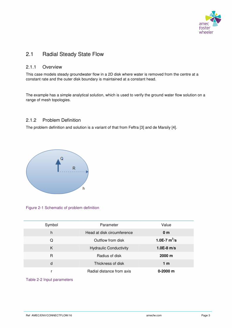
This case models steady groundwater flow in a 2D disk where water is removed from the centre at a constant rate and the outer disk boundary is maintained at a constant head.
The example has a simple analytical solution, which is used to verify range of mesh topologies.
2.1.2 Problem Definition
The problem definition and solution is a variant of that from Feftra [
Figure 2-1 Schematic of problem definition
Symbol
h
Q
K
R
d
r
Table 2-2 Input parameters
amecfw.com
Radial Steady State Flow
This case models steady groundwater flow in a 2D disk where water is removed from the centre at a constant rate and the outer disk boundary is maintained at a constant head.
The example has a simple analytical solution, which is used to verify the ground water flow solution on a
The problem definition and solution is a variant of that from Feftra [3] and de Marsily [
lem definition
Parameter Value
Head at disk circumference 0 m
Outflow from disk 1.0E-7 m
Hydraulic Conductivity 1.0E-8 m/s
Radius of disk 2000 m
Thickness of disk 1 m
Radial distance from axis 0-2000 m
Page 3
This case models steady groundwater flow in a 2D disk where water is removed from the centre at a
the ground water flow solution on a
] and de Marsily [4].
Value
0 m
7 m3/s
8 m/s
2000 m
1 m
2000 m

Ref AMEC/ENV/CONNECTFLOW/16
2.1.3 Variations
2.1.3.1 Mass flux boundary condition
The modelled domain consists of a 15 degree sector, which is truncated at r = 1 m where a mass flux boundary condition is applied. The mesh consists of a line of 3Drefined towards the centre of the domain.
Figure 2-2 Hexahedral mesh with sector truncated close to origin
2.1.3.2 Point sink and prism element
The modelled domain consists of a 15 degree sector, which is composed of a line of hexahedral elements except at the origin where a prism element is used. The outflow is modelled using point sinks at the two vertices on the axis.
Figure 2-3 Hexahedral mesh with prism at origin
2.1.4 Constrained mesh
The modelled domain consists of a 15 degree sector, which is truncated at r = 1 m, where a mass flux boundary is applied. The mesh consists of a line of 3D hexahedral elements for r = 1 m to r mesh is then refined into two cells circumferentially from r = 1000 m to r = 2000 m. The meshes are joined using ConnectFlow constraints. This is an advanced technique that allows grids of different densities to be connected together.
Figure 2-4 Hexahedral constrained mesh
amecfw.com
Mass flux boundary condition
The modelled domain consists of a 15 degree sector, which is truncated at r = 1 m where a mass flux boundary condition is applied. The mesh consists of a line of 3D hexahedral elements, with the spacing refined towards the centre of the domain.
Hexahedral mesh with sector truncated close to origin
Point sink and prism element
of a 15 degree sector, which is composed of a line of hexahedral elements except at the origin where a prism element is used. The outflow is modelled using point sinks at the two
Hexahedral mesh with prism at origin
The modelled domain consists of a 15 degree sector, which is truncated at r = 1 m, where a mass flux boundary is applied. The mesh consists of a line of 3D hexahedral elements for r = 1 m to r mesh is then refined into two cells circumferentially from r = 1000 m to r = 2000 m. The meshes are joined using ConnectFlow constraints. This is an advanced technique that allows grids of different densities to be
Hexahedral constrained mesh
Page 4
The modelled domain consists of a 15 degree sector, which is truncated at r = 1 m where a mass flux hexahedral elements, with the spacing
of a 15 degree sector, which is composed of a line of hexahedral elements except at the origin where a prism element is used. The outflow is modelled using point sinks at the two
The modelled domain consists of a 15 degree sector, which is truncated at r = 1 m, where a mass flux boundary is applied. The mesh consists of a line of 3D hexahedral elements for r = 1 m to r = 1000 m. The mesh is then refined into two cells circumferentially from r = 1000 m to r = 2000 m. The meshes are joined using ConnectFlow constraints. This is an advanced technique that allows grids of different densities to be

Ref AMEC/ENV/CONNECTFLOW/16
2.1.5 Results
The analytical solution is given by
)ln(2
)()(r
R
Kd
QRhrh
π−=
The results from ConnectFlow show very good agreement with the analytical solution in Figure 2-6. The solution for the constrained mesh in
Figure 2-5 Mass flux boundary condition
-8
-7
-6
-5
-4
-3
-2
-1
0
0 500
Radius [m]
He
ad
[m
]
amecfw.com
The analytical solution is given by
The results from ConnectFlow show very good agreement with the analytical solution in . The solution for the constrained mesh in Figure 2-7 is a little less accurate as expected.
Mass flux boundary condition
1000 1500 2000
Radius [m]
ConnectFlow
Analytical Solution
Page 5
The results from ConnectFlow show very good agreement with the analytical solution in Figure 2-5 and is a little less accurate as expected.
ConnectFlow
Analytical Solution

Ref AMEC/ENV/CONNECTFLOW/16
Figure 2-6 Point sink and prism element
Figure 2-7 Constrained mesh
-8
-7
-6
-5
-4
-3
-2
-1
0
0 500
Head
[m
]
-8
-7
-6
-5
-4
-3
-2
-1
0
0 500
Head
[m
]
amecfw.com
Point sink and prism element
1000 1500 2000
Radius [m]
ConnectFlow
Analytical Solution
1000 1500 2000
Radius [m]
ConnectFlow
Analytical Solution
Page 6
ConnectFlow
Analytical Solution
ConnectFlow
Analytical Solution

Ref AMEC/ENV/CONNECTFLOW/16
2.2 Steady Flow in Fractured Rock
2.2.1 Overview
This case is taken from Level 1 of the international HYDROCOIN project flow codes [5]. It models steady state flow in a twocontains two inclined fractures which intersect one another at depth, and have a higher permeability than the surrounding rock.
The topography has been made simple so that it consists of two valleys located where the fracture zones meet the surface. To simplify the problem definition, the shape of the surface is described by straight lines. Although the surface topography is symmetric, the flow is influenced by the asymmetry of the fracture zones.
This problem is based on an idealized version of the hydrogeological conditions encountered at a potential site for a deep repository in Swedish bedrock. A detailed threeseparate study [6].
2.2.2 Problem Definition
Figure 2-8 depicts the modelled domain.
Figure 2-8 Fractured rock
amecfw.com
Steady Flow in Fractured Rock
This case is taken from Level 1 of the international HYDROCOIN project for verification of groundwater ]. It models steady state flow in a two-dimensional vertical slice of fractured rock. The rock
contains two inclined fractures which intersect one another at depth, and have a higher permeability than
The topography has been made simple so that it consists of two valleys located where the fracture zones meet the surface. To simplify the problem definition, the shape of the surface is described by straight lines.
hy is symmetric, the flow is influenced by the asymmetry of the fracture
This problem is based on an idealized version of the hydrogeological conditions encountered at a potential site for a deep repository in Swedish bedrock. A detailed three-dimensional model of this was made in a
depicts the modelled domain.
Page 7
for verification of groundwater dimensional vertical slice of fractured rock. The rock
contains two inclined fractures which intersect one another at depth, and have a higher permeability than
The topography has been made simple so that it consists of two valleys located where the fracture zones meet the surface. To simplify the problem definition, the shape of the surface is described by straight lines.
hy is symmetric, the flow is influenced by the asymmetry of the fracture
This problem is based on an idealized version of the hydrogeological conditions encountered at a potential sional model of this was made in a

Ref AMEC/ENV/CONNECTFLOW/16
Symbol
Kr Hydraulic conductivity of rock
Kf
φ
Table 2-3 Input parameters
2.2.3 Variations
2.2.3.1 Multiple Element Types
In this variation the region is meshed using a mix of hexahedral (CB27) and prismatic elements as shown in Figure 2-9.
Figure 2-9 Mesh around fractures
amecfw.com
Parameter Value
Hydraulic conductivity of rock 1.0E-8 m/s
Hydraulic conductivity of fracture
1.0E-6 m/s
Porosity 0.03
In this variation the region is meshed using a mix of hexahedral (CB27) and prismatic elements as shown
Page 8
Value
8 m/s
6 m/s
0.03
In this variation the region is meshed using a mix of hexahedral (CB27) and prismatic elements as shown

Ref AMEC/ENV/CONNECTFLOW/16
2.2.3.2 Hexahedral Elements
In this variant hexahedral elements only are used, and then the element permeabilties are modified according to the imported fractures. It was found that in this scenario the lower ora more accurate solution than the CB27 elements for a given mesh resolution. This is likely to be due to the rapid change in permeabilties that are not aligned with the grid.
The results presented here are for mesh with 160x80 elemethis approach is illustrated in Figure
Figure 2-10 Hexahedral elements
2.2.4 Results
The results presented here compare head profile at a height of y=show excellent agreement with the HYDROCOIN study. The hexahedral element results have a head profile that is close to the HYDROCOIN results, but with slightly higher heads across the range.
amecfw.com
In this variant hexahedral elements only are used, and then the element permeabilties are modified according to the imported fractures. It was found that in this scenario the lower order CB08 elements gave a more accurate solution than the CB27 elements for a given mesh resolution. This is likely to be due to the rapid change in permeabilties that are not aligned with the grid.
The results presented here are for mesh with 160x80 elements. The representation of the fractures using Figure 2-10.
The results presented here compare head profile at a height of y=-200. The multiple element type results show excellent agreement with the HYDROCOIN study. The hexahedral element results have a head
he HYDROCOIN results, but with slightly higher heads across the range.
Page 9
In this variant hexahedral elements only are used, and then the element permeabilties are modified der CB08 elements gave
a more accurate solution than the CB27 elements for a given mesh resolution. This is likely to be due to
nts. The representation of the fractures using
200. The multiple element type results show excellent agreement with the HYDROCOIN study. The hexahedral element results have a head
he HYDROCOIN results, but with slightly higher heads across the range.

Ref AMEC/ENV/CONNECTFLOW/16
Figure 2-11 Head at height -200m (multiple element types)
Figure 2-12 Head at height -200m (hexahedral element mesh)
In addition, the ConnectFlow results were compared against the Feftra base case results reported in [The differences in head between the two codes being less than 1% for the multiple element type mesh and less than 2% for the hexahedral mesh (relative to the head variation in the surface boundary condition).
100
105
110
115
120
125
0 400
Distance [m]
Head
[m
]
100
105
110
115
120
125
0 400
Distance [m]
Head
[m
]
amecfw.com
200m (multiple element types)
200m (hexahedral element mesh)
In addition, the ConnectFlow results were compared against the Feftra base case results reported in [rences in head between the two codes being less than 1% for the multiple element type mesh and
less than 2% for the hexahedral mesh (relative to the head variation in the surface boundary condition).
800 1200 1600
Distance [m]
ConnectFlow
Hydrocoin
800 1200 1600
Distance [m]
ConnectFlow
Hydrocoin
Page 10
In addition, the ConnectFlow results were compared against the Feftra base case results reported in [3]. rences in head between the two codes being less than 1% for the multiple element type mesh and
less than 2% for the hexahedral mesh (relative to the head variation in the surface boundary condition).
ConnectFlow
Hydrocoin
ConnectFlow
Hydrocoin

Ref AMEC/ENV/CONNECTFLOW/16
A particle track starting from position (100,as illustrated in Figure 2-13.
Figure 2-13 Particle track from (100
In Figure 2-14 the ConnectFlow particle track is overlaid on the geometry, with the track colouring representing elapsed time. The total time of the track is 5% hig
Figure 2-14 Particle track overlaid on geometry
-700
-600
-500
-400
-300
-200
-100
0
100
200
0 200 400
Y m
amecfw.com
A particle track starting from position (100,-200) also showed good agreement with the Feftra base case,
Particle track from (100,-200) with multiple element types
the ConnectFlow particle track is overlaid on the geometry, with the track colouring otal time of the track is 5% higher than the Feftra base case.
Particle track overlaid on geometry
600 800 1000 1200 1400
X m
Page 11
showed good agreement with the Feftra base case,
the ConnectFlow particle track is overlaid on the geometry, with the track colouring her than the Feftra base case.
ConnectFlow
Feftra

Ref AMEC/ENV/CONNECTFLOW/16
2.3 2D Steady Flow with Particle Tracks
2.3.1 Overview
This case is taken from Level 3 of the flow codes [7]. It models steady state flow in a tworegion of higher permeability.
The case has a non-uniform analytical solution antracking.
2.3.2 Problem Definition
The analytical solution assumes an infinite domain for the low permeability region. The original HYDROCOIN setup had a disk radius acalculated and analytically prescribed flow fields.
In the ConnectFlow results presented here both the flow field and particle tracks are calculated. From initial tests it was found that a larger outer region was required in order to appropriatanalytical solution.
Figure 2-15 Schematic of problem definition
Symbol
Lx
Ly Vertical outer region distance
a
P1
P0
ko
ki
φ
ρ
µ
Table 2-4 Input parameters
amecfw.com
2D Steady Flow with Particle Tracks
This case is taken from Level 3 of the international HYDROCOIN project for verification of groundwater ]. It models steady state flow in a two-dimensional vertical slice of rock, containing a circular
uniform analytical solution and is used in the HYDROCOIN study to test particle
solution assumes an infinite domain for the low permeability region. The original HYDROCOIN setup had a disk radius a = 10m, an outer region Lx = 50m, Ly = 30m ancalculated and analytically prescribed flow fields.
In the ConnectFlow results presented here both the flow field and particle tracks are calculated. From initial tests it was found that a larger outer region was required in order to appropriat
Schematic of problem definition
Parameter Value
Upstream and downstream distances
250 m
Vertical outer region distance 240 m
Radius of inner disk 10 m
Upstream pressure 2.5E5 Pa
Downstream pressure -2.5E5 Pa
Permeability of outer region 1.0E-15 m
Permeability of inner region 1.0E-13 m
Porosity 0.1
Density 1000 kg/m
Viscosity 1.0E-3 Pa.s
Page 12
international HYDROCOIN project for verification of groundwater dimensional vertical slice of rock, containing a circular
d is used in the HYDROCOIN study to test particle
solution assumes an infinite domain for the low permeability region. The original 10m, an outer region Lx = 50m, Ly = 30m and used both
In the ConnectFlow results presented here both the flow field and particle tracks are calculated. From initial tests it was found that a larger outer region was required in order to appropriately model the
Value
250 m
240 m
10 m
2.5E5 Pa
2.5E5 Pa
15 m2
13 m2
0.1
1000 kg/m3
3 Pa.s

Ref AMEC/ENV/CONNECTFLOW/16
Eight particle tracks are released 50 m upstream of the disk centre and at Y values of 10, 12, 14, 16, 18, 20, 22 and 24 m.
The analytical solution for the pathlines is given in the HYDROCOIN report [
)1/()(
)(2
2
oi
oi
kk
kk
r
aoyy
+
−+= for r > a
o
oi
k
kk
oyy2
)( += for r < a
Where r is the distance from the center of the disk and ya long distance away from the origin.
2.3.3 Variations
2.3.3.1 Wrapped Mesh
In this variation, the mesh is modelled to wrap around the cylinder. A higher quality mesh is generated, but some vertices are surrounded by 3 elements and others by 5. A mesh of around 3000 elements was used.
Figure 2-16 Wrapped mesh
The mesh topology does not support the mass conserving particle tracking method, so just the regular particle tracking approach was used.
amecfw.com
Eight particle tracks are released 50 m upstream of the disk centre and at Y values of 10, 12, 14, 16, 18,
analytical solution for the pathlines is given in the HYDROCOIN report [7] as
distance from the center of the disk and y0 is a constant representing the height of the track a long distance away from the origin.
In this variation, the mesh is modelled to wrap around the cylinder. A higher quality mesh is generated, but some vertices are surrounded by 3 elements and others by 5. A mesh of around 3000 elements was used.
The mesh topology does not support the mass conserving particle tracking method, so just the regular particle tracking approach was used.
Page 13
Eight particle tracks are released 50 m upstream of the disk centre and at Y values of 10, 12, 14, 16, 18,
is a constant representing the height of the track
In this variation, the mesh is modelled to wrap around the cylinder. A higher quality mesh is generated, but some vertices are surrounded by 3 elements and others by 5. A mesh of around 3000 elements was used.
The mesh topology does not support the mass conserving particle tracking method, so just the regular

Ref AMEC/ENV/CONNECTFLOW/16
2.3.3.2 Regular Mesh (Distorted Elements)
In this variation a regular mesh is used where elemdistorted mesh inside the cylindrical region. A mesh of around 6000 elements was used. The mesh is finer in this case, as the refinement of the cylinder propagates to the boundaries.
Figure 2-17 Regular mesh
Both regular particle tracking and the mass conserving method were used.
2.3.4 Results
The calculated particle tracks were within 1% of the analytical solution, both in terms of location at each point and in terms of overall travel from x =
Calculation method
Wrapped mesh, regular tracks
Regular mesh, regular tracks
Regular mesh, mass conserving tracks
Table 2-5 Particle tracking results
amecfw.com
Regular Mesh (Distorted Elements)
In this variation a regular mesh is used where elements always have 4 neighbours, which results in a distorted mesh inside the cylindrical region. A mesh of around 6000 elements was used. The mesh is finer in this case, as the refinement of the cylinder propagates to the boundaries.
Both regular particle tracking and the mass conserving method were used.
The calculated particle tracks were within 1% of the analytical solution, both in terms of location at each in terms of overall travel from x = -50m to x = +50m.
% Error in Location % Error in Travel Time
0.96% 0.44%
0.41% 0.17%
0.27% 0.20%
Page 14
ents always have 4 neighbours, which results in a distorted mesh inside the cylindrical region. A mesh of around 6000 elements was used. The mesh is finer
The calculated particle tracks were within 1% of the analytical solution, both in terms of location at each
% Error in Travel Time
0.44%
0.17%
0.20%

Ref AMEC/ENV/CONNECTFLOW/16
Backward particle tracks from x = 50m to x = analytical values.
Calculation method
Wrapped mesh, regular tracks
Regular mesh, regular tracks
Regular mesh, mass conserving tracks
Table 2-6 Backward particle tracking results
Figure 2-18 Particle tracks for wrapped mesh
In addition, the volumetric flow rate through the inner disk was calculated for variation 1, using the “calculate conserved mass flux” option.
The flow through the disk from [7] has a constant velocity in the X direction of
the values in Table 2-4, this gives a flow rate of 1.9801E1.9834E-7 m3/s which is within 1% of the analytical solution.
amecfw.com
Backward particle tracks from x = 50m to x = -50m were also calculated and were again within 1% of the
% Error in Location % Error in Travel Time
0.93% 0.45%
0.41% 0.17%
0.27% 0.21%
Backward particle tracking results
Particle tracks for wrapped mesh
In addition, the volumetric flow rate through the inner disk was calculated for variation 1, using the “calculate conserved mass flux” option.
] has a constant velocity in the X direction of ( i
o
k
k
+
, this gives a flow rate of 1.9801E-7 m3/s. The calculated ConnectFlow value is /s which is within 1% of the analytical solution.
Page 15
50m were also calculated and were again within 1% of the
ror in Travel Time
0.45%
0.17%
0.21%
In addition, the volumetric flow rate through the inner disk was calculated for variation 1, using the
)( )
µϕxo
io
L
PP
k
k
2
01−
+. For
/s. The calculated ConnectFlow value is

Ref AMEC/ENV/CONNECTFLOW/16
2.4 Transient Buoyant Flow
2.4.1 Overview
This case is taken from Level 1 of theflows [5]. It models the flows arising from an exponentially decaying heat source and has an asolution.
This type of problem is relevant when considering the disposal of heat emitting radioactive waste, where buoyancy induced flows can last for thousands of years.
2.4.2 Problem Definition
Figure 2-19 Schematic of problem definition
The test problem models transient heat flow through the rock only and ignores advection of heat. The viscosity is taken to be constant and the density variation is only applied to the buoyancyequations.
The modelled domain consists of a thin one cell thick segment of the sphere. The analytical solution assumes an unbounded region of surrounding rock. Following some initial test runs, a surrounding region of 12000 m was selected as having a minimal impact on the solution.
A relatively fine mesh of 26000 elements was used. Coarser meshes of around 5000 elements give good results for the temperature and pressure profiles but have larger errors on particle tracking positions and travel times.
amecfw.com
Transient Buoyant Flow
This case is taken from Level 1 of the international HYDROCOIN project for the verification of groundwater ]. It models the flows arising from an exponentially decaying heat source and has an a
This type of problem is relevant when considering the disposal of heat emitting radioactive waste, where buoyancy induced flows can last for thousands of years.
Schematic of problem definition
The test problem models transient heat flow through the rock only and ignores advection of heat. The viscosity is taken to be constant and the density variation is only applied to the buoyancy
The modelled domain consists of a thin one cell thick segment of the sphere. The analytical solution assumes an unbounded region of surrounding rock. Following some initial test runs, a surrounding region
having a minimal impact on the solution.
A relatively fine mesh of 26000 elements was used. Coarser meshes of around 5000 elements give good results for the temperature and pressure profiles but have larger errors on particle tracking positions and
Page 16
international HYDROCOIN project for the verification of groundwater ]. It models the flows arising from an exponentially decaying heat source and has an analytical flow
This type of problem is relevant when considering the disposal of heat emitting radioactive waste, where
The test problem models transient heat flow through the rock only and ignores advection of heat. The viscosity is taken to be constant and the density variation is only applied to the buoyancy term of the
The modelled domain consists of a thin one cell thick segment of the sphere. The analytical solution assumes an unbounded region of surrounding rock. Following some initial test runs, a surrounding region
A relatively fine mesh of 26000 elements was used. Coarser meshes of around 5000 elements give good results for the temperature and pressure profiles but have larger errors on particle tracking positions and

Ref AMEC/ENV/CONNECTFLOW/16
Symbol
W0
λ
rρ
C
rΓ
k
φ
Ss
ρ
µ
β
Table 2-7 Input parameters
2.4.3 Results
The comparison of results includes temperature profiles transient particle tracks Figure 2-22
The results are all within 7% of the analytical solution, including the particle travel times.
amecfw.com
Parameter Value
Initial power output 250 MW
Decay constant in heat source 7.3215E
Rock density 2.6E3 kg/m
Rock specific heat 8.79E2 J/kg K
Rock thermal conductivity 2.51 W/m K
Permeability 1.0E
Porosity 1.0E
Specific storage coefficient 2.0E
Density 992.2 kg/m
Viscosity 6.529E
Expansion coefficient of water 3.85E
The comparison of results includes temperature profiles Figure 2-20, pressure profiles 22 and Figure 2-23.
of the analytical solution, including the particle travel times.
Page 17
Value
250 MW
7.3215E-10 1/s
2.6E3 kg/m3
8.79E2 J/kg K
2.51 W/m K
1.0E-16 m2
1.0E-4
2.0E-6 1/m
992.2 kg/m3
6.529E-4 Pa.s
3.85E-4 1/K
, pressure profiles Figure 2-21 and
of the analytical solution, including the particle travel times.

Ref AMEC/ENV/CONNECTFLOW/16
Figure 2-20 Vertical temperature rise along the vertical sphere centreline
Figure 2-21 Vertical pressure rise along the vertical sphere centreline
0.0
10.0
20.0
30.0
40.0
50.0
60.0
70.0
80.0
90.0
0 200
Radius [m]
Tem
pera
ture
Ris
e [
K]
0
2000
4000
6000
8000
10000
12000
14000
16000
18000
20000
0 200
Radius [m]
Pre
ssu
re R
ise [
Pa]
amecfw.com
Vertical temperature rise along the vertical sphere centreline
Vertical pressure rise along the vertical sphere centreline
400 600 800
Radius [m]
ConnectFlow t=50
Analytical t=50
ConnectFlow t=100
Analytical t=100
ConnectFlow t=500
Analytical t=500
ConnectFlow t=1000
Analytical t=1000
400 600 800
Radius [m]
ConnectFlow t=50
Analytical t=50
ConnectFlow t=100
Analytical t=100
ConnectFlow t=500
Analytical t=500
ConnectFlow t=1000
Analytical t=1000
Page 18
ConnectFlow t=50
Analytical t=50
ConnectFlow t=100
Analytical t=100
ConnectFlow t=500
Analytical t=500
ConnectFlow t=1000
Analytical t=1000
ConnectFlow t=50
Analytical t=50
ConnectFlow t=100
Analytical t=100
ConnectFlow t=500
Analytical t=500
ConnectFlow t=1000
Analytical t=1000

Ref AMEC/ENV/CONNECTFLOW/16
Figure 2-22 Particle tracks originating from z = 0 starting at t = 100 years
Figure 2-23 Particle tracks originating from z = 0 starting at t = 1000 years
-400
-200
0
200
400
600
800
1000
0 500
Radius [m]
z [
m]
-400
-200
0
200
400
600
800
1000
0 500
Radius [m]
z [
m]
amecfw.com
Particle tracks originating from z = 0 starting at t = 100 years
Particle tracks originating from z = 0 starting at t = 1000 years
500 1000
Radius [m]
ConnectFlow r = 125 m
Analytic r = 125 m
ConnectFlow r = 250 m
Analytic r = 250 m
Sphere
1000
Radius [m]
ConnectFlow r = 125 m
Analytic r = 125 m
ConnectFlow r = 250 m
Analytic r = 250 m
Sphere
Page 19
ConnectFlow r = 125 m
Analytic r = 125 m
ConnectFlow r = 250 m
Analytic r = 250 m
ConnectFlow r = 125 m
Analytic r = 125 m
ConnectFlow r = 250 m
Analytic r = 250 m

Ref AMEC/ENV/CONNECTFLOW/16
2.5 Unsaturated Heat Transport
2.5.1 Overview
In this section, the base-case modelSystems (EBS) Task Force [ 8 ] is investigated. A model, including the bentonite buffer and the host rock. The canister is not explicitly representedheat source term is applied on a canister buffer interface. Emphasis of the analysis is othe temperature and saturation with time along fixed positions on the bentonite buffer.
2.5.2 Problem Definition
The deposition hole is based on the KBSand its features are schematically illustrated in
Figure 2-24 Dimensions of the computational domain (dark grey is the host rock, light grey is the bentonite yellow is the area of canister.
The modelling process is subdivided into two phases (i.e. Phase 1 and Phase 2). Phase 1 hydraulic calculation and considers an open deposition hole (i.e. with the canister and bentoniteDirichlet boundary conditions (BCs) (i.e. atmospheric pressure) and on the upper anis applied along the axis of symmetry and at the initial condition (IC) throughout the rest of the state is reached. Phase 1 providescoupled Thermo – hydraulic calculation. The numerical simulation the canister and bentonite buffer within the deposition hole 1 For the purposes of this verification exercise, the thermal conductivity of the buffer is assumed to be constant rather than a function of saturation (i.e.
description for the base-case model.
amecfw.com
Unsaturated Heat Transport
case model1of the Sensitivity Analysis Task of the Äspö Engineered Barrier is investigated. A single deposition hole is modelled in a 2D axisymmetric
model, including the bentonite buffer and the host rock. The canister is not explicitly representedheat source term is applied on a canister buffer interface. Emphasis of the analysis is othe temperature and saturation with time along fixed positions on the bentonite buffer.
ole is based on the KBS-3V [ 8 ] specifications. Dimensions of the computational domain and its features are schematically illustrated in Figure 2-24.
of the computational domain (dark grey is the host rock, light grey is the bentonite yellow is the area of canister. This figure is reproduced from [8]
The modelling process is subdivided into two phases (i.e. Phase 1 and Phase 2). Phase 1 considers an open deposition hole (i.e. with the canister and bentonite
(BCs) for the pressure are specified on the surface of the depositi(i.e. atmospheric pressure) and on the upper and lower boundaries of the model. Ais applied along the axis of symmetry and at the other outer boundaries. Hydrostatic pressure is set as an
throughout the rest of the domain and a transient simulation is performed untilprovides the steady state pressure field for Phase 2, as an IC. Phas
calculation. The numerical simulation begins on the date of emplacement of the canister and bentonite buffer within the deposition hole, and a transient calculation is performed for
For the purposes of this verification exercise, the thermal conductivity of the buffer is assumed to be
constant rather than a function of saturation (i.e. ( ) ll SS ⋅+−⋅ 3.117.0 W/(m·K)) prescribed in the Task
case model.
Page 20
Engineered Barrier single deposition hole is modelled in a 2D axisymmetric
model, including the bentonite buffer and the host rock. The canister is not explicitly represented; instead a heat source term is applied on a canister buffer interface. Emphasis of the analysis is on the variation of the temperature and saturation with time along fixed positions on the bentonite buffer.
specifications. Dimensions of the computational domain
of the computational domain (dark grey is the host rock, light grey is the bentonite
The modelling process is subdivided into two phases (i.e. Phase 1 and Phase 2). Phase 1 is a purely considers an open deposition hole (i.e. with the canister and bentonite absent).
the surface of the deposition hole A Neumann ‘no-flow’ BC,
Hydrostatic pressure is set as an simulation is performed until steady
as an IC. Phase 2 is a on the date of emplacement of
a transient calculation is performed for
For the purposes of this verification exercise, the thermal conductivity of the buffer is assumed to be
) prescribed in the Task

Ref AMEC/ENV/CONNECTFLOW/16
100 years after the installation. The at the outer edge of the canister –heat generated by nuclear fuel wasteThe initial power output ��is 1700
���� � �� ∑ �� exp �� �
���
The ICs and BCs employed in the modelling ofThe physical parameters used in the modelling
Figure 2-25 Summary of the ICs and BCs
amecfw.com
100 years after the installation. The BCs applied in Phase 1 are used, with the addit– bentonite interface. A heat source applied at the interface
nuclear fuel waste. The power decay used in the modelling is given by Equatiis 1700 W, whilst parameters it and ia are listed in Table
the modelling of both phases are schematically summarisedused in the modelling are presented in Table 2-9 and Table
Summary of the ICs and BCs for Phase 1 and Phase 2.
Page 21
with the addition of a Neumann BC e applied at the interface emulates the
given by Equation (1). Table 2-8.
�1�
ses are schematically summarised in Figure 2-25. Table 2-10.

Ref AMEC/ENV/CONNECTFLOW/16
The standard Van Genuchten model (
2-10 for the host rock), is fully implemented bentonite buffer, a modified Van Genuchten functionTable 2-10). In addition, a cubic law relating the relative permeability and the saturation is also prescribed. This functionality is easily implemented in ConnectFlow with the aid of two user defined external routinesuspcap.f and uskrel.f. These versatile
In total, the grid consists of approximately 2500 bentonite buffer, the canister – bentonite interface, as well as the points used for the sampling of temperature and saturation are presented.
I
1
2
3
4
5
6
7
Table 2-8 Constants and coefficients for the power output from the canister
amecfw.com
The standard Van Genuchten model (i.e. the functional forms ( )capl
PS , )(lrel
Sk
fully implemented in ConnectFlow. The task specifications require thata modified Van Genuchten function, is to be used (with an extra term i
a cubic law relating the relative permeability and the saturation is also prescribed. mplemented in ConnectFlow with the aid of two user defined external routinesse versatile routines enable the user to freely specify the relationships used
the grid consists of approximately 2500 finite elements. In Figure 2-26, the discretisation along the bentonite interface, as well as the points used for the sampling of
temperature and saturation are presented.
ti (years) �� 20 0.0601
50 0.7050
200 -0.0547
500 0.249
2000 0.0254
5000 -0.0094
20000 0.023
and coefficients for the power output from the canister, as described in Equation (1)
Page 22
), as presented in Table
specifications require that, for the extra term in (�����,�� ) in
a cubic law relating the relative permeability and the saturation is also prescribed. mplemented in ConnectFlow with the aid of two user defined external routines,
the relationships used.
, the discretisation along the bentonite interface, as well as the points used for the sampling of
0.0601
0.7050
0.0547
0.2498
0.0254
0.0094
0.0239
as described in Equation (1)

Ref AMEC/ENV/CONNECTFLOW/16
Parameter
Fluid Properties
Density ( lρ )
Viscosity ( lµ )
Host Rock Properties
Density (Rρ )
Porosity (Rn )
Initial Liquid Saturation ( 0,lS )
Capillary Pressure ( capRP , )
Relative permeability (liquid) ( relRk ,
Tortuosity�!"� Bentonite Properties
Density (Bρ )
Porosity (Bn )
Initial Liquid Saturation ( 0,lS )
Capillary Pressure ( capBP , )
Tortuosity (Bτ )
Relative permeability (liquid) ( relBk ,
Table 2-9 Thermodynamic, transport and hydraulic properties, are presented for the fluidand the bentonite buffer
amecfw.com
Value
1000 kg / m3
1.0 x 10⁻³ Pa·s
2700 kg / m3
0.003
1.0
) ( ) cap
caplP
PPS
−+=
0
1
P0 = 1.74 MPa, m=0.60
rel )
1
11)(
−−=
m
m
lllrelSSSk
m=0.6
1.0
2780 kg / m3
0.438
0.61
( )1
1
0
,
,1
mcapB
capBlP
PPS
−+=
−
−
P0 = 5.523 MPa, m=0.16, P1 = 950 MPa, m1=1.6.
1.0
lrel, ) 3lS
Thermodynamic, transport and hydraulic properties, are presented for the fluidand the bentonite buffer
Page 23
m
m
−
−
1
1
,
=0.60
2
,
1
1
,1
m
capB
m
P
P
+
=1.6.
Thermodynamic, transport and hydraulic properties, are presented for the fluid, the host rock

Ref AMEC/ENV/CONNECTFLOW/16
Parameter
Thermal conductivity ( lλ )
Specific heat capacity ( lc )
Host
Thermal conductivity ( Rλ )
Specific heat capacity ( Rc )
Bentonite Properties
Thermal conductivity (Bλ )
Specific heat capacity ( Bc
Table 2-10 Thermal properties of the
2.5.3 Results
In Figure 2-27, a series of surface plots of the temperature distribution (Phase 2 calculation)different times are displayed. The temperature variation is shown for the whole extent of the comdomain. The Task Description, prescribes six sampling pointcollection of temperature and saturation measurements.are directly compared to ones obtained by(Figure 2-28) and saturation profiles (ConnectFlow is found to be smaller by few degreeson the slope of saturation rate, full saturation is achieved for all points at approximately the same timeConnectFlow predicting a fully saturated state at
Deviations are to be expected. Even though the same grnumerical solution scheme is adoptedis opted for ConnectFlow. In particulardifferent. TOUGH2 uses a multiphase calculation[11]. Within this investigation, emphasis was placed simulation, thus an approximation to Richards equation.
amecfw.com
Value
Fluid Properties
0.6 W/(m·K)
) 4.183 kJ/(kg·K)
Host Rock Properties
) 2.4 W/(m·K)
) 770 J/(kg·K)
Bentonite Properties
) 1.2 W/(m·K)
B ) 800 J/(kg·K)
hermal properties of the fluid, the host rock and the buffer.
, a series of surface plots of the temperature distribution (Phase 2 calculation). The temperature variation is shown for the whole extent of the com
The Task Description, prescribes six sampling points (see Figure 2-26) to be used for the collection of temperature and saturation measurements. In this study, results obtained using ConnectFlow
to ones obtained byTOUGH2. A good agreement is shown forration profiles (Figure 2-29). The maximum temperature achieved for
ler by few degrees. However, even though there is a moderate deviation l saturation is achieved for all points at approximately the same time
ConnectFlow predicting a fully saturated state at slightly earlier times.
ven though the same grid is used for both computationserical solution scheme is adopted in TOUGH2 (i.e. Finite Difference), while the Finite Element method
In particular, the set of equations solved by ConnectFlow and TOUGH2 are multiphase calculation, whilst ConnectFlow solves Richards
emphasis was placed on the minimisation of gas effects within, thus an approximation to Richards equation is justified.
Page 24
, a series of surface plots of the temperature distribution (Phase 2 calculation) collected at . The temperature variation is shown for the whole extent of the computational
) to be used for the obtained using ConnectFlow
good agreement is shown for both temperature achieved for all points by
there is a moderate deviation l saturation is achieved for all points at approximately the same time, with
id is used for both computations, a different while the Finite Element method
by ConnectFlow and TOUGH2 are s Richards equation [9], [10] &
minimisation of gas effects within the TOUGH2

Ref AMEC/ENV/CONNECTFLOW/16
Figure 2-26 Part of the mesh used discretisation of the buffer. Temperature and saturation profiles are obtained for the six points in the buffer and presented in layer (red elements) between the canister and the buffer is shown.
.
Figure 2-27 The temperature field in the
amecfw.com
used for the computations is given in the figure on the leftdiscretisation of the buffer. Temperature and saturation profiles are obtained for the six
and presented in Figure 2-28 & Figure 2-29. On the right, the interfacelayer (red elements) between the canister and the buffer is shown.
ture field in the model is plotted at different times.
Page 25
n the figure on the left, showing the discretisation of the buffer. Temperature and saturation profiles are obtained for the six
. On the right, the interface

Ref AMEC/ENV/CONNECTFLOW/16
Figure 2-28 Variation of Temperature with time, simulations.
Figure 2-29 Variation of Saturation with time, simulations.
amecfw.com
iation of Temperature with time, calculated by ConnectFlow (�) and TOUGH2(
Variation of Saturation with time, calculated by ConnectFlow (�) and TOUGH2(
Page 26
) and TOUGH2(- -)
) and TOUGH2(- -)

Ref AMEC/ENV/CONNECTFLOW/16
2.6 1D Transient Unsaturated Flow
2.6.1 Overview
This case models transient flow in a 50 m horizontal section of clay, where the initiaand the ends are maintained at a different pressure.
For small variations in pressure the problem has a semi
2.6.2 Problem Definition
Figure 2-30 Schematic of problem
The region was meshed using a line of 40 hexahedral elements.
The unsaturated behaviour for relative permeability and capillary pressure were modelled using Van Genuchten functions.
Symbol
K
φ
Ss
ρ
µ
Van Genuchten
n
Pr
Slr
Table 2-11 Input parameter values
amecfw.com
1D Transient Unsaturated Flow
This case models transient flow in a 50 m horizontal section of clay, where the initiaand the ends are maintained at a different pressure.
For small variations in pressure the problem has a semi-analytical solution.
Schematic of problem definition
The region was meshed using a line of 40 hexahedral elements.
The unsaturated behaviour for relative permeability and capillary pressure were modelled using Van
Parameter Value
Hydraulic Conductivity 5.0E
Porosity 0.18
Specific storage coefficient 2.0E
Density 1000 kg/m
Viscosity 1.0E
Exponent
Entry pressure 8.0E6 Pa
Residual Saturation 0.01
Input parameter values
Page 27
This case models transient flow in a 50 m horizontal section of clay, where the initial pressure is constant
The unsaturated behaviour for relative permeability and capillary pressure were modelled using Van
Value
5.0E-14 m/s
0.18
2.0E-6 1/m
1000 kg/m3
1.0E-3 Pa.s
1.5
8.0E6 Pa
0.01

Ref AMEC/ENV/CONNECTFLOW/16
As the variation in saturation across the model is small (<3%), we can approximate the equations for transient unsaturated flow as a diffusion
2
2
x
P
t
P
∂
∂=
∂
∂α
where
α is the diffusivity [m
x is distance [m];
P is pressure;
t is time.
and α is given by
P
SgSS
Kk
s
r
∂
∂+
=
φρ
α
where S is the liquid saturation and
For the case considered here, the values in the above equation are averaged between the initial conditions and the boundary conditions to provide an approximate constant diffusivity.
Given this approximate constant diffusivity, a semi
( )( )∑
∞
= +−+=
0
101 exp12
4
n nPPPP
π
Where Po is the uniform initial pressure field domain length of 50 m.
amecfw.com
As the variation in saturation across the model is small (<3%), we can approximate the equations for transient unsaturated flow as a diffusion equation, so that, in 1D
is the diffusivity [m2s-1];
is distance [m];
where S is the liquid saturation and rk is the relative permeability and g is gravity.
For the case considered here, the values in the above equation are averaged between the initial conditions and the boundary conditions to provide an approximate constant diffusivity.
constant diffusivity, a semi-analytical solution can be obtained from
( ) ( )
+
+−
2
2212
sin12
expL
xn
L
tn παπ
is the uniform initial pressure field -1.1E7, P1 the boundary pressure of -1.0E7, and
Page 28
As the variation in saturation across the model is small (<3%), we can approximate the equations for
For the case considered here, the values in the above equation are averaged between the initial conditions
analytical solution can be obtained from
1.0E7, and L the

Ref AMEC/ENV/CONNECTFLOW/16
2.6.3 Variations
2.6.3.1 Crank Nicholson
The transient behaviour is modelled using Crank Nicholson with 150 time steps of size 1.0E11 seconds.
2.6.3.2 Gears method
The transient behaviour is modelled using Gears predictortime step of 1.0E11 seconds. A total of
2.6.4 Results
The results show good agreement with the semisemi-analytical model assuming constant saturation with time.
Figure 2-31 Crank Nicholson - Transient unsaturated pressures
-1.08E+07
-1.07E+07
-1.06E+07
-1.05E+07
-1.04E+07
-1.03E+07
-1.02E+07
-1.01E+07
-1.00E+07
0 10 20
Distance [m]
Resid
ual
Pre
ssu
re [
Pa]
amecfw.com
transient behaviour is modelled using Crank Nicholson with 150 time steps of size 1.0E11 seconds.
The transient behaviour is modelled using Gears predictor-corrector time stepping method with an initial time step of 1.0E11 seconds. A total of 23 time steps were used.
The results show good agreement with the semi-analytical solution. The small differences are due to the analytical model assuming constant saturation with time.
Transient unsaturated pressures
30 40 50
Distance [m]
ConnectFlow 5.0E12 seconds
Semi analytical 5.0E12 seconds
ConnectFlow 1.0E13 seconds
Semi analytical 1.0E13 seconds
ConnectFlow 5.0E13 seconds
Semi analytical 5.0E13 seconds
Page 29
transient behaviour is modelled using Crank Nicholson with 150 time steps of size 1.0E11 seconds.
corrector time stepping method with an initial
analytical solution. The small differences are due to the
ConnectFlow 5.0E12 seconds
Semi analytical 5.0E12 seconds
ConnectFlow 1.0E13 seconds
Semi analytical 1.0E13 seconds
ConnectFlow 5.0E13 seconds
Semi analytical 5.0E13 seconds

Ref AMEC/ENV/CONNECTFLOW/16
Figure 2-32 Gears method - Transient unsaturated pressures
An additional comparison was made with Tough2v2 software [
Calculation method
ConnectFlow – Crank Nicholson
ConnectFlow – Gears Method
Semi analytical
Tough2
Table 2-12 Comparison with Tough2v2
Both ConnectFlow and Tough2 show the same behaviour relative to the semi analytical solution.
-1.08E+07
-1.07E+07
-1.06E+07
-1.05E+07
-1.04E+07
-1.03E+07
-1.02E+07
-1.01E+07
-1.00E+07
0 10 20
Distance [m]
Resid
ual
Pre
ssu
re [
Pa]
amecfw.com
Transient unsaturated pressures
An additional comparison was made with Tough2v2 software [12].
Pressure at x=25, t=1.0E13
Crank Nicholson -1.0426E7
Gears Method -1.0421E7
-1.0438E7
-1.0423E7
Comparison with Tough2v2
Both ConnectFlow and Tough2 show the same behaviour relative to the semi analytical solution.
30 40 50
Distance [m]
ConnectFlow 5.0E12 seconds
Semi analytical 5.0E12 seconds
ConnectFlow 1.0E13 seconds
Semi analytical 1.0E13 seconds
ConnectFlow 5.0E13 seconds
Semi analytical 5.0E13 seconds
Page 30
Pressure at x=25, t=1.0E13
Both ConnectFlow and Tough2 show the same behaviour relative to the semi analytical solution.
ConnectFlow 5.0E12 seconds
Semi analytical 5.0E12 seconds
ConnectFlow 1.0E13 seconds
Semi analytical 1.0E13 seconds
ConnectFlow 5.0E13 seconds
Semi analytical 5.0E13 seconds

Ref AMEC/ENV/CONNECTFLOW/16
2.7 Seepage Face
2.7.1 Overview
A seepage face is a boundary between the saturated flow field and the atmosphere, along which groundwater discharges. A seepage face iDirichlet boundary condition (BC) head#(set to be equal to the elevation i.e. $ � 0). The BC along the ground surface above the upper limit (a point for a 2D models or a line in 3D models) of the seepage face, is usually a Neumann BC (i.e. no flow). The challenge in modelling a seepage face is that its upper extent is unknown during the problem formulation and its determination forms a part of the solution. This verification case considers the steady state radial flow to a well, for which the Dupuit –Forchheimer well discharge formula holds (analytical solutioassumptions) [13].
2.7.2 Problem Definition
A schematic diagram of the problem (segment of a cylinder) is presented inpolar coordinate system �&, '�, the well axis is aligned with the imposed at the bottom and the top of the model. A far distance himposed on the right of the model, setting up the initial height of the water table (i.e. head BC (# � #(), is imposed at the bottom of the well (blue line) . Along the side of the well (red line)seepage face boundary condition is applied. The resulting flow is radially symmetric between the circular equipotential boundaries located at
Figure 2-33 Schematic illustration of seepage face.
amecfw.com
A seepage face is a boundary between the saturated flow field and the atmosphere, along which groundwater discharges. A seepage face is homologous to a free surface boundary condition, so a
suffices for its mathematical description, either in terms of hydraulic (set to be equal to the elevation ' i.e. # � '), or in terms of total pressure $
). The BC along the ground surface above the upper limit (a point for a 2D models or a line in 3D models) of the seepage face, is usually a Neumann BC (i.e. no flow). The challenge in modelling a
extent is unknown during the problem formulation and its determination This verification case considers the steady state radial flow to a well, for which
Forchheimer well discharge formula holds (analytical solution based on the Dupuit
A schematic diagram of the problem (segment of a cylinder) is presented in Figure , the well axis is aligned with the ' axis. A no-flow boundary condition is
imposed at the bottom and the top of the model. A far distance head boundary condition (green line) is imposed on the right of the model, setting up the initial height of the water table (i.e.
), is imposed at the bottom of the well (blue line) . Along the side of the well (red line)seepage face boundary condition is applied. The resulting flow is radially symmetric between the circular equipotential boundaries located at & � ) and & � &(.
Schematic illustration of the conceptual model of a steady state radial flow to a well with a
Page 31
A seepage face is a boundary between the saturated flow field and the atmosphere, along which s homologous to a free surface boundary condition, so a
suffices for its mathematical description, either in terms of hydraulic $ (set to atmospheric
). The BC along the ground surface above the upper limit (a point for a 2D models or a line in 3D models) of the seepage face, is usually a Neumann BC (i.e. no flow). The challenge in modelling a
extent is unknown during the problem formulation and its determination This verification case considers the steady state radial flow to a well, for which
n based on the Dupuit
Figure 2-33. In a cylindrical flow boundary condition is
ead boundary condition (green line) is imposed on the right of the model, setting up the initial height of the water table (i.e. # � #*), whilst a fixed
), is imposed at the bottom of the well (blue line) . Along the side of the well (red line), a seepage face boundary condition is applied. The resulting flow is radially symmetric between the circular
the conceptual model of a steady state radial flow to a well with a

Ref AMEC/ENV/CONNECTFLOW/16
For the above configuration and based on the Dupuit assumptionssteady volumetric discharge into the well can be derived. This expression known as the Dupuit Forchheimer well discharge formula, is given as:
+, � -. /012 /,2345" 6,7 8 .
Further, the phreatic surface elevation
/ � 9:�6�, where :�6� �
Symbol
.
ρ
µ
/,
/*
6,
"
Table 2-13 Input parameters.
.
2.7.3 Variations
2.7.3.1 Volumetric discharge
The first verification test involves the direct comparison of the volumetic flow rates to the well, as obtained by ConnectFlow, to the ones suggested by the Dupuitapproach incorporates a thin wedge shapedapproximation to the conceptual axissymetric model. Three flow domains are investigated. For each case, only the radius of the domain ) is altered (i.e. computational domain, the radius of the well, the head at the elevation of the well and the initial head of the aquifer are kept fixed as, ; �seepage face BC as implemented within Conin Figure 2-33). The next task, takes into account the performance of the implemented BC, by investigatihow closely the head approximates the elevation along the seepage face, as well as the recovery of the length of the seepage face.
amecfw.com
For the above configuration and based on the Dupuit assumptions [13] , an analytical expression for the steady volumetric discharge into the well can be derived. This expression known as the Dupuit Forchheimer well discharge formula, is given as:
8 .
Further, the phreatic surface elevation # � #�&� is given as:
� � � /,2 < �/∞2 � /,2 � =>5" 67 8
=>5" 6,7 8.
Parameter Value
Hydraulic conductivity 9.81E-7 m/s
Density 1000.0 kg/m3
Viscosity 1.0E-3 Pa.s
Hydraulic Head at the well 100 m
Initial water table 450 m
Radius of the well 50 m
Radius of influence i)1000 m ii)2000 m iii)3000 m
The first verification test involves the direct comparison of the volumetic flow rates to the well, as obtained by ConnectFlow, to the ones suggested by the Dupuit- Forchheimer well discharge formula. The modelling approach incorporates a thin wedge shaped computational domain in ConnectFlow, which serves as an approximation to the conceptual axissymetric model. Three flow domains are investigated. For each case,
is altered (i.e. ) � 1000, 2000, 3000ABC� ,whilst the heightcomputational domain, the radius of the well, the head at the elevation of the well and the initial head of
800ABC, &( � 50ABC, #( � 100ABC and #* � 450seepage face BC as implemented within ConnectFlow, is applied along the periphery of the well (red line
). The next task, takes into account the performance of the implemented BC, by investigatihow closely the head approximates the elevation along the seepage face, as well as the recovery of the
Page 32
lytical expression for the steady volumetric discharge into the well can be derived. This expression known as the Dupuit –
( 1 )
( 2 )
Value
i)1000 m ii)2000 m iii)3000
The first verification test involves the direct comparison of the volumetic flow rates to the well, as obtained Forchheimer well discharge formula. The modelling
computational domain in ConnectFlow, which serves as an approximation to the conceptual axissymetric model. Three flow domains are investigated. For each case,
,whilst the height of the computational domain, the radius of the well, the head at the elevation of the well and the initial head of
450ABC, respectively. The nectFlow, is applied along the periphery of the well (red line
). The next task, takes into account the performance of the implemented BC, by investigating how closely the head approximates the elevation along the seepage face, as well as the recovery of the

Ref AMEC/ENV/CONNECTFLOW/16
2.7.4 Results
The results in terms of volumetric flow rates (solution (1) are in a good agreement. In particular it can be observed that an increase in the aspect ratio defined as the radius of influence
Radius of the domain
Aspect Ratio" 6,7
" � GHHHAIC 20
" � 2HHHAIC 40
" � JHHHAIC 60
Table 2-14 Volumetic flow rates to the well, calculated using the Dupuit ConnecFlow, for different radius of influence.
Considering the actual performance of the seepage face BC, it can be observed from along the length of the seepage face (selength of the seepage face is shown to be sensitive to the radius of influence, which appears to decrease with an increasing radius of influence. boundary of the well, and further supplements the above observation. Clearly the upper extent of the seepage face (position where the flowincreasing radius of influence. In Table presented, where it is also accompanied by the relative error of the computed head with respect to the actual elevation. Evidently, in all three cases the error is below #~') and a satisfactory performance for
Figure 2-34 On the left graph the Head is plotted as function of the elevation, whilst the figure on the right displays the fraction of the elevation over the head, as function of the elevation.
amecfw.com
olumetric flow rates (Table 2-14), as obtained by ConnectFlow and the analytical solution (1) are in a good agreement. In particular it can be observed that an increase in the aspect ratio defined as the radius of influence over the radius of the well, results in more accurate prediction
Aspect Ratio
7Dupuit-Forchheimer
IJL7
ConnectFlow IJ
L7
0.1980 0.1672
0.1608 0.1472
0.1448 0.1378
Volumetic flow rates to the well, calculated using the Dupuit –Forchheimer formula and ConnecFlow, for different radius of influence.
Considering the actual performance of the seepage face BC, it can be observed from along the length of the seepage face (see Table 2-15), the head closely approximates the elevation. The length of the seepage face is shown to be sensitive to the radius of influence, which appears to decrease
ius of influence. Figure 2-35, portrays the behaviour of the saturation along the boundary of the well, and further supplements the above observation. Clearly the upper extent of the seepage face (position where the flow is fully saturated i.e. � � 1), is found to be decreasing with an
Table 2-15, the position of the upper extent of the seepage facepresented, where it is also accompanied by the relative error of the computed head with respect to the actual elevation. Evidently, in all three cases the error is below 1%, suggesting a good approximation (i.e.
) and a satisfactory performance for the BC.
On the left graph the Head is plotted as function of the elevation, whilst the figure on the right displays the fraction of the elevation over the head, as function of the elevation.
Page 33
), as obtained by ConnectFlow and the analytical solution (1) are in a good agreement. In particular it can be observed that an increase in the aspect ratio
over the radius of the well, results in more accurate prediction.
Abosulute Error %
3.0804
1.3551
0.7035
Forchheimer formula and
Considering the actual performance of the seepage face BC, it can be observed from Figure 2-34 that ), the head closely approximates the elevation. The
length of the seepage face is shown to be sensitive to the radius of influence, which appears to decrease , portrays the behaviour of the saturation along the
boundary of the well, and further supplements the above observation. Clearly the upper extent of the ), is found to be decreasing with an
, the position of the upper extent of the seepage face is presented, where it is also accompanied by the relative error of the computed head with respect to the
, suggesting a good approximation (i.e.
On the left graph the Head is plotted as function of the elevation, whilst the figure on the right displays the fraction of the elevation over the head, as function of the elevation.

Ref AMEC/ENV/CONNECTFLOW/16
Radius of the
domain
Aspect Ratio
" 6,7
" � GHHHAIC 20
" � 2HHHAIC 40
" � JHHHAIC 60
Table 2-15 The upper extent of the seepage face, its actual length and the mean value of the relative error along the whole extent of the seepage face, measuring the performance of the seepage face BC.
Figure 2-35 Saturation N, along the well boundary is plotted as function of the elevation.
The computed phreatic surfaces obtained for the three flow domains, are grouped and presented, along with the ones obtained after applying the DupuitFigure 2-36. It must be noted that within the Dupuit assumptions the seepage face is neglected, and that the analytical approximation is only valid far from the well. As can be seen, the computed phreatic surface closely resembles the one obtained from Dupuit of depression is found to be decreasing as the radius of influence decreases.
amecfw.com
Aspect Ratio
7
Upper extent of the
seepage face
AIC
Seepage face
length
AIC
340 90
320 70
310 60
The upper extent of the seepage face, its actual length and the mean value of the relative error along the whole extent of the seepage face, measuring the performance of the seepage
, along the well boundary is plotted as function of the elevation.
The computed phreatic surfaces obtained for the three flow domains, are grouped and presented, along with the ones obtained after applying the Dupuit-Forchheimer model (see equation 2 ) are presented in
. It must be noted that within the Dupuit assumptions the seepage face is neglected, and that the analytical approximation is only valid far from the well. As can be seen, the computed phreatic surface
y resembles the one obtained from Dupuit – Forchheimer for increasing values of of depression is found to be decreasing as the radius of influence decreases.
Page 34
Mean Relative
Error
�/ � OO �%
0.3348
0.2888
0.2641
The upper extent of the seepage face, its actual length and the mean value of the relative error along the whole extent of the seepage face, measuring the performance of the seepage
, along the well boundary is plotted as function of the elevation.
The computed phreatic surfaces obtained for the three flow domains, are grouped and presented, along Forchheimer model (see equation 2 ) are presented in
. It must be noted that within the Dupuit assumptions the seepage face is neglected, and that the analytical approximation is only valid far from the well. As can be seen, the computed phreatic surface
Forchheimer for increasing values of &. Finally, the cone

Ref AMEC/ENV/CONNECTFLOW/16
Figure 2-36 Water table position, based on the computations (lines) and the Dupuit Forchheimer model (squares).
amecfw.com
osition, based on the computations (lines) and the Dupuit Forchheimer model
Page 35
osition, based on the computations (lines) and the Dupuit Forchheimer model

Ref AMEC/ENV/CONNECTFLOW/16
2.8 Henry’s Salt Transport
2.8.1 Overview
This case considers salt water intrusion into a vertical slice of an isotropic homogeneous confined aquifer.
The variant modelled is a modified version of the original Henry‘s test case, as recommended in [modified case halves the fresh water inflow rate, which increases the sensitivity of the solution to the variation in density.
2.8.2 Problem Definition
A schematic of the test case is shown in
Figure 2-37 Henry's Problem
A uniform hexahedral grid was used of size 80x40 elements.
Symbol
K Hydraulic conductivity of rock
D
Q
0ρ
maxρ
Lα
Tα
φ
amecfw.com
Henry’s Salt Transport
This case considers salt water intrusion into a vertical slice of an isotropic homogeneous confined aquifer.
led is a modified version of the original Henry‘s test case, as recommended in [modified case halves the fresh water inflow rate, which increases the sensitivity of the solution to the
st case is shown in Figure 2-37 and the input parameters are given in
A uniform hexahedral grid was used of size 80x40 elements.
Parameter Value
Hydraulic conductivity of rock 1.0E-2 m/s
Coefficient of molecular diffusion
1.886E-5 m
Freshwater inflow per unit depth
3.3E-5 m
Reference density 998 kg/m
Saltwater density 1023 kg/m
Longitudinal dispersivity 0 m
Transverse dispersivity 0 m
Porosity 0.35
Page 36
This case considers salt water intrusion into a vertical slice of an isotropic homogeneous confined aquifer.
led is a modified version of the original Henry‘s test case, as recommended in [14]. The modified case halves the fresh water inflow rate, which increases the sensitivity of the solution to the
and the input parameters are given in Table 2-16.
Value
2 m/s
5 m2/s
5 m2/s
998 kg/m3
1023 kg/m3
0 m
0 m
0.35

Ref AMEC/ENV/CONNECTFLOW/16
Table 2-16 Input parameters
The model makes use of the ConnectFlow “reference waters” capability which allows fluids with different properties to be defined. The steady solution is obtained by running a transient solstate is reached.
2.8.3 Results
The test case has an analytical solution, represented by an infinite double Fourier series. A truncated form of the series gives a non-linear system which can then be iteratively solved. Results from this preported in [14] and these are used for the comparisons in location is less than 3%.
Figure 2-38 Non-dimensional concentration of salinity
0.00
0.10
0.20
0.30
0.40
0.50
0.60
0.70
0.80
0.90
1.00
0.00 0.20 0.40 0.60
y [
m]
ConnectFlow 25%
Semi analytical 25%
ConnectFlow 50%
Semi analytical 50%
ConnectFlow 75%
Semi analytical 75%
amecfw.com
The model makes use of the ConnectFlow “reference waters” capability which allows fluids with different properties to be defined. The steady solution is obtained by running a transient solution until the steady
The test case has an analytical solution, represented by an infinite double Fourier series. A truncated form linear system which can then be iteratively solved. Results from this p
] and these are used for the comparisons in Figure 2-38. The maximum error in contour
dimensional concentration of salinity
0.60 0.80 1.00 1.20 1.40 1.60 1.80 2.00
X [m]
ConnectFlow 25%
Semi analytical 25%
ConnectFlow 50%
Semi analytical 50%
ConnectFlow 75%
Semi analytical 75%
Page 37
The model makes use of the ConnectFlow “reference waters” capability which allows fluids with different ution until the steady
The test case has an analytical solution, represented by an infinite double Fourier series. A truncated form linear system which can then be iteratively solved. Results from this process are
. The maximum error in contour
2.00
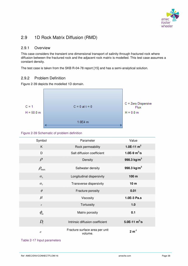
Ref AMEC/ENV/CONNECTFLOW/16
2.9 1D Rock Matrix Diffusion (RMD)
2.9.1 Overview
This case considers the transient one diffusion between the fractured rock and the adjacent rock matrix is modelled. This test case assumes a constant density.
The test case is taken from the SKB R
2.9.2 Problem Definition
Figure 2-39 depicts the modelled 1D domain.
Figure 2-39 Schematic of problem
Symbol
K
D
ρ
maxρ
Lα
Tα
φ
µ
τ
mφ
iD
σ Fracture surface area per unit
Table 2-17 Input parameters
amecfw.com
1D Rock Matrix Diffusion (RMD)
This case considers the transient one dimensional transport of salinity through fractured rock where diffusion between the fractured rock and the adjacent rock matrix is modelled. This test case assumes a
The test case is taken from the SKB R-04-78 report [15] and has a semi-analytical solution.
depicts the modelled 1D domain.
Schematic of problem definition
Parameter Value
Rock permeability 1.0E-11 m
Salt diffusion coefficient 1.0E-9 m
Density 998.3 kg/m
Saltwater density 998.3 kg/m
Longitudinal dispersivity 100 m
Transverse dispersivity 10 m
Fracture porosity 0.01
Viscosity 1.0E-3 Pa.s
Tortuosity 1.0
Matrix porosity 0.1
Intrinsic diffusion coefficient 5.0E-11 m
Fracture surface area per unit volume.
2 m-1
Page 38
dimensional transport of salinity through fractured rock where diffusion between the fractured rock and the adjacent rock matrix is modelled. This test case assumes a
nalytical solution.
Value
11 m2
9 m2/s
998.3 kg/m3
998.3 kg/m3
100 m
10 m
0.01
3 Pa.s
11 m2/s
1

Ref AMEC/ENV/CONNECTFLOW/16
In this case the rock matrix diffusion slows down the increaseproportion of the salinity is diffusing into the surrounding rock matrix. The time taken for the midrelative concentration to reach 0.99 is increased by more than a factor 10 due to RMD.
2.9.3 Variations
2.9.3.1 Crank Nicholson
In this variation the non-linear system is solved using Newton iteration on each time step for all variables as a single group. Automatic time stepping is used to gradually increase the time step size from its initial value of 1.0E6 seconds.
2.9.3.2 Sequential Inner Iteration
Sequential inner iteration solves the nonto a user-specified sequence of Newton iterations on subgroups of the full system of equations. In this test the pressure field is time independent, so just the salt concentration is solved for.
This setup also uses nodal quadrature in order to allow an optimized fast equation assembly process. Both the fast assembly and normal assembly were tested.
Automatic time stepping is used to gradually increase the time step size from its initial value of 1.0E6 seconds.
2.9.3.3 Increased Salt Diffusion Coefficient
The effective dispersion of concentration is given by
)( vD
Lατ
ϕρ +
Where v is the pore water velocity in the fractured rock, which for this case has a constant value of
4.981E-5 m/s. This means that τ
D
This variation sets the dispersion length
results in a modified test with the same effective diffusion and hence the same semi
amecfw.com
In this case the rock matrix diffusion slows down the increase in salinity in the fractured rock, as a proportion of the salinity is diffusing into the surrounding rock matrix. The time taken for the midrelative concentration to reach 0.99 is increased by more than a factor 10 due to RMD.
linear system is solved using Newton iteration on each time step for all variables as a single group. Automatic time stepping is used to gradually increase the time step size from its initial
tial Inner Iteration
Sequential inner iteration solves the non-linear system of equations that arise at each time step according specified sequence of Newton iterations on subgroups of the full system of equations. In this test
is time independent, so just the salt concentration is solved for.
This setup also uses nodal quadrature in order to allow an optimized fast equation assembly process. Both the fast assembly and normal assembly were tested.
sed to gradually increase the time step size from its initial value of 1.0E6
Increased Salt Diffusion Coefficient
The effective dispersion of concentration is given by
is the pore water velocity in the fractured rock, which for this case has a constant value of
D = 1.0E-9 and vLα = 4.981E-3.
This variation sets the dispersion length Lα to zero, and the salt diffusion coefficient D to 4.981E
results in a modified test with the same effective diffusion and hence the same semi
Page 39
in salinity in the fractured rock, as a proportion of the salinity is diffusing into the surrounding rock matrix. The time taken for the mid-point relative concentration to reach 0.99 is increased by more than a factor 10 due to RMD.
linear system is solved using Newton iteration on each time step for all variables as a single group. Automatic time stepping is used to gradually increase the time step size from its initial
linear system of equations that arise at each time step according specified sequence of Newton iterations on subgroups of the full system of equations. In this test
This setup also uses nodal quadrature in order to allow an optimized fast equation assembly process. Both
sed to gradually increase the time step size from its initial value of 1.0E6
is the pore water velocity in the fractured rock, which for this case has a constant value of
to zero, and the salt diffusion coefficient D to 4.981E-3. This
results in a modified test with the same effective diffusion and hence the same semi-analytical solution.

Ref AMEC/ENV/CONNECTFLOW/16
2.9.3.4 Finite Volume RMD
This variant uses the alternative finite volume RMD method indiscretisation of the rock matrix into a 1D column of cells at each solution node in the model. The discretisation is specified by the user, e.g. reasonable accuracy for a given level of refinement.compatible with reactive transport. The model used for verification is thmatrix porosity of 0.3.
Figure 2-40 Schematic of the distribution of cell sizes in the rock matrix
2.9.4 Results
The semi-analytical solution is derived using Laplace transforms, which are then inverted numerically. The details of this process are covered in [
The results show good agreement with the swithin 1% of the semi-analytical solution for all variations. The concentration profiles for three time values are shown in Figure 2-41.
Fracture
Original distribution (x = D/5)
Distribution 2 (x = D/15)
Distribution 3 (x = D/15)
Distribution 4 (x = D/21)
Distribution 5 (x = D/31)
amecfw.com
This variant uses the alternative finite volume RMD method in ConnectFlow that provides an explicit discretisation of the rock matrix into a 1D column of cells at each solution node in the model. The discretisation is specified by the user, e.g. Figure 2-40. This method provides computational efficiency with reasonable accuracy for a given level of refinement. Unlike the original RMD method, this method is compatible with reactive transport. The model used for verification is the same as the base case, but with a
Schematic of the distribution of cell sizes in the rock matrix.
derived using Laplace transforms, which are then inverted numerically. The details of this process are covered in [15].
The results show good agreement with the semi-analytical solution, the ConnectFlow concentrations being analytical solution for all variations. The concentration profiles for three time values
Rock matrix Fracture
x 2x 3x 4x 5x
x 2x 4x 6x 8x
x 2x 4x 8x 16
5x 4x 3x 2x x
x x x x x
D
Page 40
ConnectFlow that provides an explicit discretisation of the rock matrix into a 1D column of cells at each solution node in the model. The
This method provides computational efficiency with Unlike the original RMD method, this method is
e same as the base case, but with a
derived using Laplace transforms, which are then inverted numerically. The
analytical solution, the ConnectFlow concentrations being analytical solution for all variations. The concentration profiles for three time values

Ref AMEC/ENV/CONNECTFLOW/16
The results for the finite volume RMD method are shown in agreement with the analytical solution, but accuracy increases as the cell sizes closest to the fracture decrease in size, either due to an increase in the number of cells or by using a distribution tin cell size with distance from the fracture.
Figure 2-41 Crank Nicholson - Relative concentration
0.00E+00
1.00E-01
2.00E-01
3.00E-01
4.00E-01
5.00E-01
6.00E-01
7.00E-01
8.00E-01
9.00E-01
1.00E+00
0 2000 4000
Rela
tive C
on
cen
trati
on
0
0.1
0.2
0.3
0.4
0.5
0.6
0.7
0.8
0.9
1
0.00E+00
Re
lativ
e c
on
cent
ratio
n
FV RMD 5
FV RMD 5 (distribution 2)
FV RMD 5 (distribution 3)
amecfw.com
The results for the finite volume RMD method are shown in Figure 2-42 to Figure 2agreement with the analytical solution, but accuracy increases as the cell sizes closest to the fracture decrease in size, either due to an increase in the number of cells or by using a distribution tin cell size with distance from the fracture.
Relative concentration
4000 6000 8000 10000
Distance [m]
ConnectFlow 5.0E7 seconds
Semi analytical 5.0E7 seconds
ConnectFlow 5.0E8 seconds
Semi analytical 5.0E8 seconds
ConnectFlow 5.0E9 seconds
Semi analytical 5E9 seconds
2.00E+03
Distance (m)
FV RMD 5 (distribution 4) FV RMD 20
FV RMD 5 (distribution 5) Analytical RMD
FV RMD 10
Page 41
2-44. There is good agreement with the analytical solution, but accuracy increases as the cell sizes closest to the fracture decrease in size, either due to an increase in the number of cells or by using a distribution that increases
ConnectFlow 5.0E7 seconds
Semi analytical 5.0E7 seconds
ConnectFlow 5.0E8 seconds
Semi analytical 5.0E8 seconds
ConnectFlow 5.0E9 seconds
Semi analytical 5E9 seconds
4.00E+03
Analytical RMD

Ref AMEC/ENV/CONNECTFLOW/16
Figure 2-42 Relative concentration along the column at time t=1.0matrix diffusion (RMD) with varying number of matrix cells and different cell sizes compared to an analytical solution.
Figure 2-43 Relative fracture water concentration midway along the column against time, using finite volume rock matrix diffusion with varying number of rock matrix cells compared to an analytical solution.
0
0.1
0.2
0.3
0.4
0.5
0.6
0.7
0.8
0.9
1
0.00E+00 2.00E+09
Rel
ativ
e co
ncen
trat
ion
0
0.1
0.2
0.3
0.4
0.5
0.6
0.7
0.8
0.9
1
0.00E+00 2.00E+09
Rel
ativ
e co
ncen
trat
ion
amecfw.com
Relative concentration along the column at time t=1.0·108 s, using finite volume (FV) rock matrix diffusion (RMD) with varying number of matrix cells and different cell sizes compared to an
Relative fracture water concentration midway along the column against time, using finite volume rock matrix diffusion with varying number of rock matrix cells compared to an analytical solution.
4.00E+09 6.00E+09 8.00E+09
Time (s)
Finite volume RMD (5 cells)
Finite volume RMD (10 cells)
Finite volume RMD (20 cells)
Analytical RMD
4.00E+09 6.00E+09 8.00E+09
Time (s)
Finite volume RMD (5 cells)
Finite volume RMD (10 cells)
Finite volume RMD (20 cells)
Analytical RMD
Page 42
108 s, using finite volume (FV) rock matrix diffusion (RMD) with varying number of matrix cells and different cell sizes compared to an
Relative fracture water concentration midway along the column against time, using finite volume rock matrix diffusion with varying number of rock matrix cells compared to an analytical solution.
8.00E+09
Finite volume RMD (5 cells)
Finite volume RMD (10 cells)
Finite volume RMD (20 cells)
8.00E+09
Finite volume RMD (5 cells)
Finite volume RMD (10 cells)
Finite volume RMD (20 cells)

Ref AMEC/ENV/CONNECTFLOW/16
Figure 2-44 Relative fracture water concentration midway along the column against time, using finite volume rock matrix diffusion with varying number of rock matrix cells compared to an analytical solution.
2.10 1D Nuclide Transport with S
2.10.1 Overview
This case considers transient onesorption and decay are considered.
The test case is taken from [16] and has an analytical solution.
2.10.2 Problem Definition
Figure 2-39 depicts the modelled 1D domain.
Figure 2-45 Schematic illustration of the problem definition
amecfw.com
Relative fracture water concentration midway along the column against time, using finite volume rock matrix diffusion with varying number of rock matrix cells compared to an analytical solution.
1D Nuclide Transport with Sorption and Decay
This case considers transient one-dimensional nuclide transport due to advection and diffusion. Both sorption and decay are considered.
] and has an analytical solution.
depicts the modelled 1D domain.
Schematic illustration of the problem definition
Page 43
Relative fracture water concentration midway along the column against time, using finite volume rock matrix diffusion with varying number of rock matrix cells compared to an analytical solution.
dimensional nuclide transport due to advection and diffusion. Both

Ref AMEC/ENV/CONNECTFLOW/16
Symbol
k
U
D
Lα
Tα
Rn1
Rn2
1nλ
2nλ
τ
ρ
µ
φ
Table 2-18 Input parameters
Constant pressure boundary conditions are applied to generate the desired Darcy velocity. The modelled is 20 days which also corresponds to the half life of the parent nuclide N1.
The mesh consists of 100 CB08 elements along the length of the flow domain, and the time step is taken to be 1E4 seconds.
2.10.3 Variations
2.10.3.1 Fast Linear Transport
Four runs are carried out to illustrate the effect of sorption and decay on the solution.
► No decay or sorption
► Sorption only
► Decay only
► Sorption and decay
amecfw.com
Parameter Value
Rock permeability 1.24E-9 m
Darcy velocity 3.486E-7 m/s
Nuclide diffusion coefficient 1.162E-7
Longitudinal dispersivity 0 m
Transverse dispersivity 0 m
Retardation factor nuclide 1 2.0
Retardation factor nuclide 2 1.0
Decay constant nuclide 1 4.011E-7
Decay constant nuclide 2 1.0E-20 1/s
Tortuousity 1.0
Density 1000.0 kg/m
Viscosity 1.0E-3 Pa.s
Porosity 0.3
Constant pressure boundary conditions are applied to generate the desired Darcy velocity. The modelled is 20 days which also corresponds to the half life of the parent nuclide N1.
The mesh consists of 100 CB08 elements along the length of the flow domain, and the time step is taken
runs are carried out to illustrate the effect of sorption and decay on the solution.
Page 44
Value
9 m2
7 m/s
7m2/s
0 m
0 m
7 1/s
20 1/s
1000.0 kg/m3
3 Pa.s
Constant pressure boundary conditions are applied to generate the desired Darcy velocity. The timescale modelled is 20 days which also corresponds to the half life of the parent nuclide N1.
The mesh consists of 100 CB08 elements along the length of the flow domain, and the time step is taken
runs are carried out to illustrate the effect of sorption and decay on the solution.

Ref AMEC/ENV/CONNECTFLOW/16
2.10.3.2 Crank Nicholson
This variation repeats the sorption and decay case using the Crank Nicholson transient s
2.10.4 Results
The results show excellent agreement with the analytical solution [nuclide N1 is compared with the analytical solution for each of the four fast linear transport runs in 2-46, Figure 2-47, Figure 2-48 and
The Crank Nicholson results were very close to the Fast Transient results, with the peak daughter nuclide concentration being 1% higher and the parent nuclide concentration being identical.
Figure 2-50 shows the ConnectFlow daughter nuclide N2 concentration for the sorption and decay case.
Figure 2-46 N1 concentration with no sorption or decay
0
0.001
0.002
0.003
0.004
0.005
0.006
0.007
0.008
0.009
0.01
0 1
Co
ncen
trati
on
amecfw.com
This variation repeats the sorption and decay case using the Crank Nicholson transient s
The results show excellent agreement with the analytical solution [17]. The concentration of the parent nuclide N1 is compared with the analytical solution for each of the four fast linear transport runs in
and Figure 2-49.
The Crank Nicholson results were very close to the Fast Transient results, with the peak daughter nuclide her and the parent nuclide concentration being identical.
shows the ConnectFlow daughter nuclide N2 concentration for the sorption and decay case.
N1 concentration with no sorption or decay
2 3 4
Distance [m]
ConnectFlow
Analytical Solution
Page 45
This variation repeats the sorption and decay case using the Crank Nicholson transient solver.
]. The concentration of the parent nuclide N1 is compared with the analytical solution for each of the four fast linear transport runs in Figure
The Crank Nicholson results were very close to the Fast Transient results, with the peak daughter nuclide her and the parent nuclide concentration being identical.
shows the ConnectFlow daughter nuclide N2 concentration for the sorption and decay case.
ConnectFlow
Analytical Solution

Ref AMEC/ENV/CONNECTFLOW/16
Figure 2-47 N1 concentration with sorption only
Figure 2-48 N1 concentration with decay only
0
0.001
0.002
0.003
0.004
0.005
0.006
0.007
0.008
0.009
0.01
0 1
Co
ncen
trati
on
0
0.001
0.002
0.003
0.004
0.005
0.006
0.007
0.008
0.009
0.01
0 1
Co
ncen
trati
on
amecfw.com
N1 concentration with sorption only
N1 concentration with decay only
2 3 4
Distance [m]
ConnectFlow
Analytical Solution
2 3 4
Distance [m]
ConnectFlow
Analytical Solution
Page 46
ConnectFlow
Analytical Solution
ConnectFlow
Analytical Solution

Ref AMEC/ENV/CONNECTFLOW/16
Figure 2-49 N1 concentration with both sorption and decay
Figure 2-50 Parent and daughter concentrations for the
0
0.001
0.002
0.003
0.004
0.005
0.006
0.007
0.008
0.009
0.01
0 1
Co
ncen
trati
on
0
0.001
0.002
0.003
0.004
0.005
0.006
0.007
0.008
0.009
0.01
0 1
Co
ncen
trati
on
amecfw.com
N1 concentration with both sorption and decay
Parent and daughter concentrations for the sorption and decay case
2 3 4
Distance [m]
ConnectFlow
Analytical Solution
2 3 4
Distance [m]
Page 47
ConnectFlow
Analytical Solution
Parent - N1
Daughter - N2

Ref AMEC/ENV/CONNECTFLOW/16
2.11 Mass Flux Calculations
2.11.1 Overview
The mass conserving algorithm was originally implemented in ConnectFlow for particle tracking calculations. The fluxes generated during particle tracking are useful in their own right for calculaflux passing through a particular region of a CPM model. This verification case compares a flux calculation using the mass conserving algorithm with an analytic solution to the same problem.
2.11.2 Problem Definition
Consider the following 3D CPM model
► A regular mesh of 4 layers of 16 x 16 cuboidal (CB08) finite elements, oriented parallel to the xplane. The dimensions of each finite element are 100 m x 100 m x 100 m giving a model with dimensions 1600 m in the x and y directions and 400 m in the
► The finite elements consist of rock 1 with permeability 1x10finite elements (4 layers of 4 x 4) which consist of rock 2 with permeability 1x10²-51).
► Pressure (Dirichlet) boundary conditions are applied to the top (z=400 m) and bottom (z=0model and no-flow boundary conditions are applied to the other sides of the mpressure gradient along the z-
The symmetry of the problem allows an analytic solution to the flow through each finite element using the following expression
ρµ
Adz
dpkF =
where
A is the area = 10,000 m2.
k is the permeability
µ is the viscosity = 0.001 Ns/m
ρ is the density = 1000 kg/m
dp/dz is the pressure gradient = 250 N/m.
F is the mass flux through the element.
amecfw.com
Mass Flux Calculations
The mass conserving algorithm was originally implemented in ConnectFlow for particle tracking calculations. The fluxes generated during particle tracking are useful in their own right for calculaflux passing through a particular region of a CPM model. This verification case compares a flux calculation using the mass conserving algorithm with an analytic solution to the same problem.
Consider the following 3D CPM model,
A regular mesh of 4 layers of 16 x 16 cuboidal (CB08) finite elements, oriented parallel to the xplane. The dimensions of each finite element are 100 m x 100 m x 100 m giving a model with dimensions 1600 m in the x and y directions and 400 m in the z direction.
The finite elements consist of rock 1 with permeability 1x10-14 m2 except for a vertical column of 64 finite elements (4 layers of 4 x 4) which consist of rock 2 with permeability 1x10
Pressure (Dirichlet) boundary conditions are applied to the top (z=400 m) and bottom (z=0flow boundary conditions are applied to the other sides of the model. These provide a
-axis of 250 N/m.
The symmetry of the problem allows an analytic solution to the flow through each finite element using the
.
is the viscosity = 0.001 Ns/m2
is the density = 1000 kg/m3
dp/dz is the pressure gradient = 250 N/m.
F is the mass flux through the element.
Page 48
The mass conserving algorithm was originally implemented in ConnectFlow for particle tracking calculations. The fluxes generated during particle tracking are useful in their own right for calculating the flux passing through a particular region of a CPM model. This verification case compares a flux calculation using the mass conserving algorithm with an analytic solution to the same problem.
A regular mesh of 4 layers of 16 x 16 cuboidal (CB08) finite elements, oriented parallel to the x-y plane. The dimensions of each finite element are 100 m x 100 m x 100 m giving a model with
except for a vertical column of 64 finite elements (4 layers of 4 x 4) which consist of rock 2 with permeability 1x10-12 m2 (see Figure
Pressure (Dirichlet) boundary conditions are applied to the top (z=400 m) and bottom (z=0 m) of the odel. These provide a
The symmetry of the problem allows an analytic solution to the flow through each finite element using the

Ref AMEC/ENV/CONNECTFLOW/16
Thus the vertical flux through the finite elements of rock type 2 is 2.5 kg/s aneach of the other finite elements is 0.025 kg/s. The total flux through all of the elements in each layer is then 43.6 kg/s.
2.11.3 Results
Using the command, >> CALCULATE CONSERVED MASS FLUXsolution to this problem exactly.
Figure 2-51 The rock types used for the mass flux verification test. Red represents rock type 2 and blue denotes rock type 1. Note that the rock types are constant along the z
2.12 Reactive Transport
2.12.1 Overview
This case considers transient onechemical reactions [18]. The results are compared with equivalent calculations carried out by Phast [and contrasted with ConnectFlow calculations without reactions included.
2.12.2 Problem Definition
For each case, a horizontal column, 10 m in length and 1 m in width and height, of grid cells is considered, as shown in Figure 2-52. The grid is discretised into cells that are cells in total. The properties used are given in used by Phast leads to numerical dispersion equal to half the cell size and therefore it is necessary to take this into account when setting the dispersion lengths, although it is a small effect relative to the diffusion in these cases. The dispersion length in held constant and is uniform across the model
amecfw.com
Thus the vertical flux through the finite elements of rock type 2 is 2.5 kg/s and the vertical flux through each of the other finite elements is 0.025 kg/s. The total flux through all of the elements in each layer is
>> CALCULATE CONSERVED MASS FLUX, ConnectFlow recreates the analytic
The rock types used for the mass flux verification test. Red represents rock type 2 and blue denotes rock type 1. Note that the rock types are constant along the z-axis.
Reactive Transport
This case considers transient one-dimensional, multi-component reactive transport due to advection and ]. The results are compared with equivalent calculations carried out by Phast [
and contrasted with ConnectFlow calculations without reactions included.
e, a horizontal column, 10 m in length and 1 m in width and height, of grid cells is considered, . The grid is discretised into cells that are 0.05 m in each dimension, giving 80,000
cells in total. The properties used are given in Table 2-19. Note that the spatial discretisation schemes o numerical dispersion equal to half the cell size and therefore it is necessary to take
this into account when setting the dispersion lengths, although it is a small effect relative to the diffusion in these cases. The dispersion length in Table 2-19 includes this numerical dispersion. The fluid density is held constant and is uniform across the model.
Page 49
d the vertical flux through each of the other finite elements is 0.025 kg/s. The total flux through all of the elements in each layer is
, ConnectFlow recreates the analytic
The rock types used for the mass flux verification test. Red represents rock type 2 and blue
omponent reactive transport due to advection and ]. The results are compared with equivalent calculations carried out by Phast [19]
e, a horizontal column, 10 m in length and 1 m in width and height, of grid cells is considered, 0.05 m in each dimension, giving 80,000
. Note that the spatial discretisation schemes o numerical dispersion equal to half the cell size and therefore it is necessary to take
this into account when setting the dispersion lengths, although it is a small effect relative to the diffusion in includes this numerical dispersion. The fluid density is

Ref AMEC/ENV/CONNECTFLOW/16
The column is initially filled with a water (aqueous solution) in Then a second water with a different composition is introduced at the upstream end of the column and allowed to flow advectively into it. The flow is specified as a flux boundary condition at the inflow end of tmodel and a zero pressure boundary condition at the outflow end, which also has an outflow (zero dispersive flux) boundary condition to allow the solutes to flow advectively from the model. The advective transport velocity is 0.1 m/y and the simulation the incoming water to be advectively transported along the full length of the column, although dispersion and diffusion processes will cause some spreading out of the front. All concentrations armass fractions in kilograms per kilogram of solution (kg/kg
Figure 2-52 Column model used for verification of reactive transport, coloured by head
Symbol
k
φ
D
Lα Longitudinal dispersion length
Tα Transverse
T
µ
ρ
U
dt
nt
Table 2-19 Input parameters for reactive transport verification
amecfw.com
The column is initially filled with a water (aqueous solution) in equilibrium with one or more mineral phases. a second water with a different composition is introduced at the upstream end of the column and
allowed to flow advectively into it. The flow is specified as a flux boundary condition at the inflow end of tmodel and a zero pressure boundary condition at the outflow end, which also has an outflow (zero dispersive flux) boundary condition to allow the solutes to flow advectively from the model. The advective transport velocity is 0.1 m/y and the simulation is run for 120 years, allowing more than sufficient time for the incoming water to be advectively transported along the full length of the column, although dispersion and diffusion processes will cause some spreading out of the front. All concentrations armass fractions in kilograms per kilogram of solution (kg/kgs).
olumn model used for verification of reactive transport, coloured by head
Parameter Value
Rock permeability 1.0E-17 m
Porosity 1.0E-
Solute diffusion coefficient 1.0E-9 m
Longitudinal dispersion length 0.05 m
Transverse dispersion length 0.05 m
Temperature 25 °C
Fluid viscosity 1.0E-3 Pa.s
Fluid density 1.0E3 kg/m
Darcy velocity 1.0E-5 m/y
Time step size 1.0 y
Number of time steps 120
reactive transport verification.
Page 50
ne or more mineral phases. a second water with a different composition is introduced at the upstream end of the column and
allowed to flow advectively into it. The flow is specified as a flux boundary condition at the inflow end of the model and a zero pressure boundary condition at the outflow end, which also has an outflow (zero dispersive flux) boundary condition to allow the solutes to flow advectively from the model. The advective
is run for 120 years, allowing more than sufficient time for the incoming water to be advectively transported along the full length of the column, although dispersion and diffusion processes will cause some spreading out of the front. All concentrations are represented as
olumn model used for verification of reactive transport, coloured by head.
Value
17 m2
-4
9 m2/s
0.05 m
0.05 m
25 °C
3 Pa.s
1.0E3 kg/m3
5 m/y
1.0 y

Ref AMEC/ENV/CONNECTFLOW/16
2.12.3 Variations
2.12.3.1 Mineral Equilibration
This variant considers equilibration of a mixture of pure water and an oxygenated saline water with calcite and pyrite. It provides an example of a redox reaction. Thedissolution/precipitation and the oxidation of iron (II) and sulphide in pyrite to iron(III) and sulphate:
4PQ
4PQ
Equilibration with CO2(g) has not been considered. with a sufficient initial quantity (10.0 mol/waters are given in Table 2-20. The column is initially filled with pure water calcite and pyrite and the saline water is introduced to the upby adjusting the chloride mass fraction and prephreeqc.dat thermodynamic database is used.
pH
pe
Component mass fractions (kg/kgs)
C
Ca
Cl
Fe
Na
S
Table 2-20 Water composition for calcite and pyrite equilibration
2.12.3.2 Ion Exchange
This variant considers the reaction of a mixture of two aqueous solutions and an ion exchanger that is able to exchange cations. The reactions are defined in the standard phreeqc.dat thermodynamic databaseusing the example exchanger ‘X’. The model initially containssmall amount of potassium, and a the column. The composition of the waters is given in exchanger X with an initial quantity of 0.011 moles per kilogram of water (mol/initialised by equilibrium with the NaCl water.
amecfw.com
considers equilibration of a mixture of pure water and an oxygenated saline water with calcite It provides an example of a redox reaction. The following reactions are significant for calcite
dissolution/precipitation and the oxidation of iron (II) and sulphide in pyrite to iron(III) and sulphate:
RRST ↔ RVW < RSTVX
;RST ↔ ;W < RSTVX
�V < 14SV < 4;VS ↔ 4PQVW < 8�SYVX < 8;W
VW < SV < 4;W ↔ 4PQTW < 2;VS
(g) has not been considered. Both the calcite and pyrite are present in the model with a sufficient initial quantity (10.0 mol/kgw) such that they will not be depleted. The composition
. The column is initially filled with pure water that has been equilibratedcalcite and pyrite and the saline water is introduced to the upstream end. Both waters are charge balanced by adjusting the chloride mass fraction and pre-equilibrated with calcite and pyrite. The standard
thermodynamic database is used.
Saline water Pure water
7.00 7.00
13.00 4.00
0.00 0.00
0.00 0.00
3.55E-5 0.00
0.00 0.00
2.30E-5 0.00
0.00 0.00
ater composition for calcite and pyrite equilibration.
considers the reaction of a mixture of two aqueous solutions and an ion exchanger that is able to exchange cations. The reactions are defined in the standard phreeqc.dat thermodynamic database
. The model initially contains a sodium chloride (NaCl) small amount of potassium, and a calcium chloride (CaCl2) solution is introduced at the upstream end of the column. The composition of the waters is given in Table 2-21. The column also contains exchanger X with an initial quantity of 0.011 moles per kilogram of water (mol/kgw), whose composition is initialised by equilibrium with the NaCl water.
Page 51
considers equilibration of a mixture of pure water and an oxygenated saline water with calcite following reactions are significant for calcite
dissolution/precipitation and the oxidation of iron (II) and sulphide in pyrite to iron(III) and sulphate:
(2-1)
(2-2)
(2-3)
(2-4)
Both the calcite and pyrite are present in the model ) such that they will not be depleted. The compositions of the
that has been equilibrated with stream end. Both waters are charge balanced
equilibrated with calcite and pyrite. The standard
Pure water
7.00
4.00
0.00
0.00
0.00
0.00
0.00
0.00
considers the reaction of a mixture of two aqueous solutions and an ion exchanger that is able to exchange cations. The reactions are defined in the standard phreeqc.dat thermodynamic database,
(NaCl) solution, with a solution is introduced at the upstream end of
. The column also contains the ion ), whose composition is

Ref AMEC/ENV/CONNECTFLOW/16
pH
pe
Component mass fractions (kg/kgs)
Ca
Cl
K
Na
Table 2-21 Water composition for
2.12.3.3 Kinetic dissolution of K-feldspar
This variant considers the dissolution of Kequilibrium under the timescales of interest. Therefore, it is appropriate to model this reaction using a kinetic approach. The reactions are defined in the standard phreeqc.dat thermodynamic databasefollows:
Z[\�]TS^ < 8The model initially contains a salineof the column. The composition of the waters is given in0.02 moles of K-feldspar per kilogram of water in the model2-23. The rate expressions are contained in the thermodynamic database.
pH
pe
Component mass fractions (kg/kgs)
Al
Cl
K
Na
Si
Table 2-22 Water composition for
amecfw.com
CaCl2 water NaCl water
7.00 7.00
4.00 4.00
2.40E-4 0.00
4.25E-4 3.90E
0.00 3.91E
0.00 2.30E
ater composition for ion exchange.
feldspar
dissolution of K-feldspar, which is a slow process and so does not tend to reach equilibrium under the timescales of interest. Therefore, it is appropriate to model this reaction using a
ons are defined in the standard phreeqc.dat thermodynamic database
8;VS → ZW < [\�S;�YX < 3;Y�]SY
saline solution and a dilute acidic solution is introduced at the upstream end of the column. The composition of the waters is given in Table 2-22. There is a uniform initial quantity of
feldspar per kilogram of water in the model. The kinetic parameters are given in The rate expressions are contained in the thermodynamic database.
Dilute water Saline water
4.00 7.00
4.00 4.00
0.00 1.17E
3.09E-6 3.08E
0.00 1.69E
2.00E-6 2.00E
0.00 3.64E
ater composition for K-feldspar dissolution.
Page 52
water
7.00
4.00
0.00
-4
-5
-4
feldspar, which is a slow process and so does not tend to reach equilibrium under the timescales of interest. Therefore, it is appropriate to model this reaction using a
ons are defined in the standard phreeqc.dat thermodynamic database as
(2-5)
solution is introduced at the upstream end There is a uniform initial quantity of
The kinetic parameters are given in Table
water
7.00
4.00
-6
-3
-6
-3
-6

Ref AMEC/ENV/CONNECTFLOW/16
Parameter
Time step subdivision
Runge-Kutta subintervals
P1 P2
Tolerance
Table 2-23 Kinetic parameters for
2.12.4 Results
2.12.4.1 Mineral Equilibration
Figure 2-53 shows the mass fraction profiles for iron. Iron is not present in the initial are no plots for the ConnectFlow case without chemistry. However, iron is produced in solutiooxidation of pyrite by the oxygenated inflowing saline water. ConnectFlow and Phast are in excellent agreement in the calculation of the total amount of iron in solution. profiles for sulphate, again showing very good agreement between Phast and ConnectFlow. in good agreement for the calculated 2-55.
amecfw.com
Value
10
3
1.36E4 dm-1
0.1
1.0E-8
for K-feldspar dissolution.
shows the mass fraction profiles for iron. Iron is not present in the initial are no plots for the ConnectFlow case without chemistry. However, iron is produced in solutiooxidation of pyrite by the oxygenated inflowing saline water. ConnectFlow and Phast are in excellent agreement in the calculation of the total amount of iron in solution. Figure 2-54 shows the mass fraction profiles for sulphate, again showing very good agreement between Phast and ConnectFlow.
calculated pe values (a measure of the redox conditions), as shown in
Page 53
shows the mass fraction profiles for iron. Iron is not present in the initial waters, hence there are no plots for the ConnectFlow case without chemistry. However, iron is produced in solution during the oxidation of pyrite by the oxygenated inflowing saline water. ConnectFlow and Phast are in excellent
shows the mass fraction profiles for sulphate, again showing very good agreement between Phast and ConnectFlow. They are also
pe values (a measure of the redox conditions), as shown in Figure

Ref AMEC/ENV/CONNECTFLOW/16
Figure 2-53 Comparison of mass fraction profiles of iron for the calcite and pyrite equilibration case between ConnectFlow (CF) and Phast. Mass fractions are sampled at 0.5column.
0.0E+00
2.0E-09
4.0E-09
6.0E-09
8.0E-09
1.0E-08
1.2E-08
1.4E-08
0.0 1.0 2.0
Fe
(k
g/k
gs
)
CF chemistry 10 y
Phast 10 y
amecfw.com
Comparison of mass fraction profiles of iron for the calcite and pyrite equilibration case een ConnectFlow (CF) and Phast. Mass fractions are sampled at 0.5 m intervals along the model
2.0 3.0 4.0 5.0 6.0 7.0 8.0
Distance (m)
CF chemistry 30 y CF chemistry 120 y
Phast 30 y Phast 120 y
Page 54
Comparison of mass fraction profiles of iron for the calcite and pyrite equilibration case m intervals along the model
9.0 10.0
CF chemistry 120 y
Phast 120 y

Ref AMEC/ENV/CONNECTFLOW/16
Figure 2-54 Comparison of mass fraction profiles of sulphate for the calcite and pyrite equilibration case between ConnectFlow (CF) and Phast. Mass fractions are sampled at 0.5column.
0.0E+00
1.0E-08
2.0E-08
3.0E-08
4.0E-08
5.0E-08
0.0 1.0 2.0
Su
lph
ate
(k
g/k
gs
)
CF chemistry 10 y
Phast 10 y
amecfw.com
Comparison of mass fraction profiles of sulphate for the calcite and pyrite equilibration case between ConnectFlow (CF) and Phast. Mass fractions are sampled at 0.5 m intervals along the model
2.0 3.0 4.0 5.0 6.0 7.0 8.0
Distance (m)
CF chemistry 30 y CF chemistry 120 y
Phast 30 y Phast 120 y
Page 55
Comparison of mass fraction profiles of sulphate for the calcite and pyrite equilibration case m intervals along the model
9.0 10.0
CF chemistry 120 y
Phast 120 y

Ref AMEC/ENV/CONNECTFLOW/16
Figure 2-55 Comparison of pe profiles for the calcite and pyrite equilibration case between ConnectFlow (CF) and Phast. Values are sampled at 0.5 m intervals along the model column.
2.12.4.2 Ion Exchange
Figure 2-56 shows the mass fraction profiles of chloride for component and there is good agreement between ConnectFlow (with and without chemistry) and Phast, showing that the transport is equivalent in each calculation. for calcium. This is not present in solution initially in thmass fraction rises with time. However, its mass fraction is reduced compared to the ConnectFlow case without chemistry calculations because the calcium ions are taken up by the ion exchanger, which releases sodium and potassium ionsexchanger are shown in Figure 2-and Phast.
-6.9
-6.8
-6.7
-6.6
0.0 1.0 2.0 3.0
pe
CF chemistry 10 y
Phast 10 y
amecfw.com
Comparison of pe profiles for the calcite and pyrite equilibration case between ConnectFlow (CF) and Phast. Values are sampled at 0.5 m intervals along the model column.
shows the mass fraction profiles of chloride for three different times. This is a noncomponent and there is good agreement between ConnectFlow (with and without chemistry) and Phast, showing that the transport is equivalent in each calculation. Figure 2-57 shows the mass fraction profiles for calcium. This is not present in solution initially in the model, but as it is introduced in the CaClmass fraction rises with time. However, its mass fraction is reduced compared to the ConnectFlow case without chemistry calculations because the calcium ions are taken up by the ion exchanger, which releases sodium and potassium ions as a consequence. The corresponding profiles for calcium in the
58. There is excellent agreement between the results for ConnectFlow
3.0 4.0 5.0 6.0 7.0 8.0 9.0
Distance (m)
CF chemistry 30 y CF chemistry 120 y
Phast 30 y Phast 120 y
Page 56
Comparison of pe profiles for the calcite and pyrite equilibration case between ConnectFlow
times. This is a non-reactive component and there is good agreement between ConnectFlow (with and without chemistry) and Phast,
shows the mass fraction profiles e model, but as it is introduced in the CaCl2 water its
mass fraction rises with time. However, its mass fraction is reduced compared to the ConnectFlow case without chemistry calculations because the calcium ions are taken up by the ion exchanger, which
The corresponding profiles for calcium in the There is excellent agreement between the results for ConnectFlow
9.0 10.0
CF chemistry 120 y
Phast 120 y

Ref AMEC/ENV/CONNECTFLOW/16
Figure 2-56 Comparison of mass fraction profiles of chloride for the ion exchange case between ConnectFlow (CF), with and without chemistry, and Phast. Mass fractions are sampled at 0.5 m intervals along the model column.
3.9E-04
4.0E-04
4.1E-04
4.2E-04
4.3E-04
0.0 1.0 2.0
Cl
(kg
/kg
s)
CF chemistry 10 y
CF no chemistry 10 y
Phast 10 y
NaCl water
amecfw.com
Comparison of mass fraction profiles of chloride for the ion exchange case between ConnectFlow (CF), with and without chemistry, and Phast. Mass fractions are sampled at 0.5 m intervals
2.0 3.0 4.0 5.0 6.0 7.0 8.0
Distance (m)
CF chemistry 30 y CF chemistry 120 y
CF no chemistry 30 y CF no chemistry 120 y
Phast 30 y Phast 120 y
CaCl2 water
Page 57
Comparison of mass fraction profiles of chloride for the ion exchange case between ConnectFlow (CF), with and without chemistry, and Phast. Mass fractions are sampled at 0.5 m intervals
9.0 10.0
CF chemistry 120 y
CF no chemistry 120 y
Phast 120 y

Ref AMEC/ENV/CONNECTFLOW/16
Figure 2-57 Comparison of mass fraction profiles of calcium for the ion exchange case between ConnectFlow (CF), with and without chemistry, and Phast. Mass fractions are sampled at 0.5 m intalong the model column.
0.0E+00
5.0E-05
1.0E-04
1.5E-04
2.0E-04
2.5E-04
0.0 1.0 2.0
Ca
(k
g/k
gs
)
CF chemistry 10 y
CF no chemistry 10 y
Phast 10 y
NaCl water
amecfw.com
Comparison of mass fraction profiles of calcium for the ion exchange case between ConnectFlow (CF), with and without chemistry, and Phast. Mass fractions are sampled at 0.5 m int
3.0 4.0 5.0 6.0 7.0 8.0
Distance (m)
CF chemistry 30 y CF chemistry 120 y
CF no chemistry 30 y CF no chemistry 120 y
Phast 30 y Phast 120 y
CaCl2 water
Page 58
Comparison of mass fraction profiles of calcium for the ion exchange case between ConnectFlow (CF), with and without chemistry, and Phast. Mass fractions are sampled at 0.5 m intervals
9.0 10.0
CF chemistry 120 y
CF no chemistry 120 y
Phast 120 y

Ref AMEC/ENV/CONNECTFLOW/16
Figure 2-58 Comparison of the CaX2 distribution (in moles per kilogram of water) across the model for the ion exchange case between ConnectFlow (CF) and Phast. Quantities are sampled at 0.5 m intervals along the model column.
2.12.4.3 K-feldspar dissolution
Figure 2-59 shows the increase in the the dissolution of K-feldspar. The decrease in the amount of KFigure 2-60. There is excellent agreement between the results for ConnectFlow and Phast.
0.0E+00
1.0E-03
2.0E-03
3.0E-03
4.0E-03
5.0E-03
6.0E-03
0.0 1.0 2.0
Ca
X2 (
mo
l/k
gw
)
CF chemistry 10 y
Phast 10 y
amecfw.com
Comparison of the CaX2 distribution (in moles per kilogram of water) across the model for the ion exchange case between ConnectFlow (CF) and Phast. Quantities are sampled at 0.5 m intervals along
increase in the mass fraction of aluminium over time at three differentThe decrease in the amount of K-feldspar due to dissolution is shown in
There is excellent agreement between the results for ConnectFlow and Phast.
2.0 3.0 4.0 5.0 6.0 7.0 8.0 9.0
Distance (m)
CF chemistry 30 y CF chemistry 120 y
Phast 30 y Phast 120 y
Page 59
Comparison of the CaX2 distribution (in moles per kilogram of water) across the model for the ion exchange case between ConnectFlow (CF) and Phast. Quantities are sampled at 0.5 m intervals along
three different times due to to dissolution is shown in
There is excellent agreement between the results for ConnectFlow and Phast.
9.0 10.0
CF chemistry 120 y
Phast 120 y
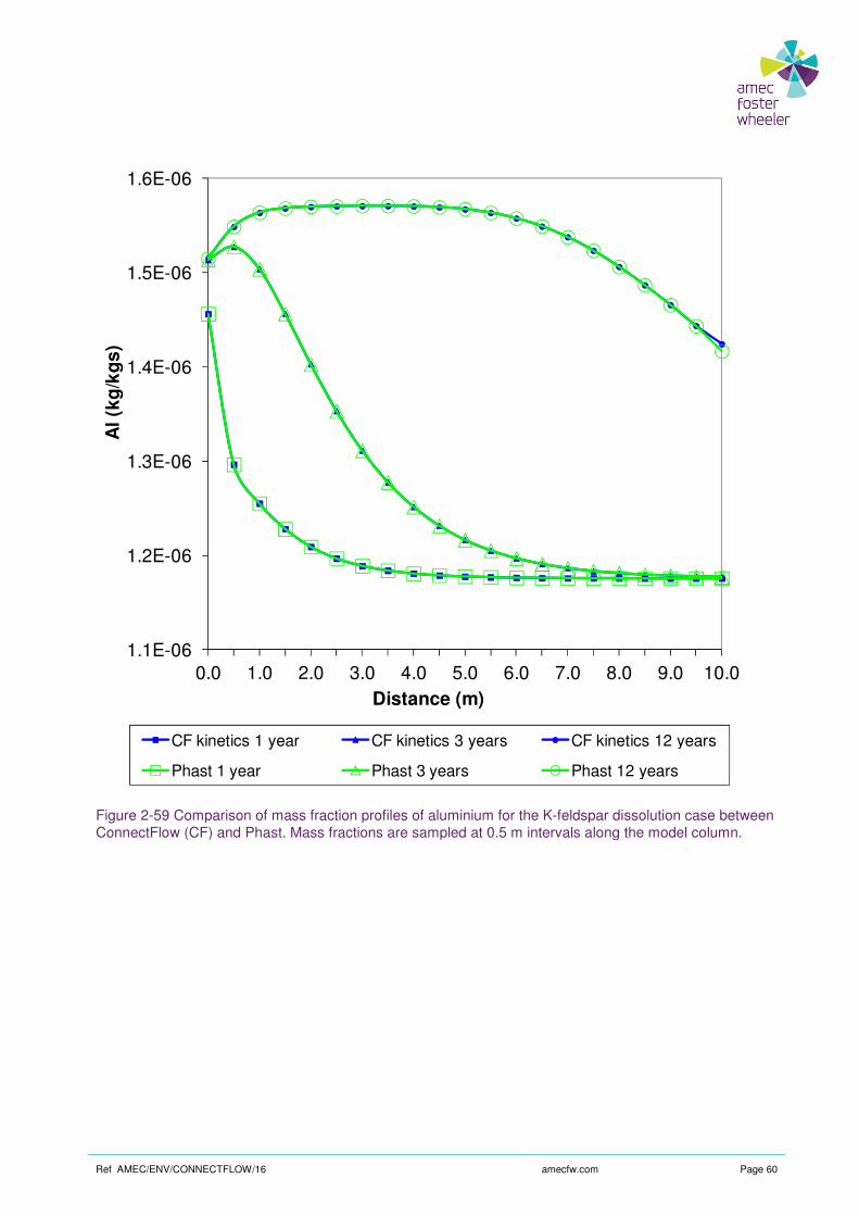
Ref AMEC/ENV/CONNECTFLOW/16
Figure 2-59 Comparison of mass fraction profiles of ConnectFlow (CF) and Phast. Mass fractions are sampled at 0.5 m intervals along the model column.
1.1E-06
1.2E-06
1.3E-06
1.4E-06
1.5E-06
1.6E-06
0.0 1.0 2.0
Al
(kg
/kg
s)
CF kinetics 1 year
Phast 1 year
amecfw.com
Comparison of mass fraction profiles of aluminium for the K-feldspar dissolutionConnectFlow (CF) and Phast. Mass fractions are sampled at 0.5 m intervals along the model column.
2.0 3.0 4.0 5.0 6.0 7.0 8.0Distance (m)
CF kinetics 3 years CF kinetics 12 years
Phast 3 years Phast 12 years
Page 60
feldspar dissolution case between ConnectFlow (CF) and Phast. Mass fractions are sampled at 0.5 m intervals along the model column.
8.0 9.0 10.0
CF kinetics 12 years
Phast 12 years

Ref AMEC/ENV/CONNECTFLOW/16
Figure 2-60 Comparison of K-feldspar quantities(CF) and Phast. Mass fractions are sampled at 0.5 m intervals along the model column.
9.5E-03
9.6E-03
9.7E-03
9.8E-03
9.9E-03
1.0E-02
0.0 1.0 2.0
K-f
eld
sp
ar
(mo
l/k
gw
)
CF kinetics 1 year
Phast 1 year
amecfw.com
feldspar quantities for the K-feldspar dissolution case between ConnectFlow (CF) and Phast. Mass fractions are sampled at 0.5 m intervals along the model column.
2.0 3.0 4.0 5.0 6.0 7.0Distance (m)
CF kinetics 1 year CF kinetics 3 years CF kinetics 12 years
Phast 3 years Phast 12 years
Page 61
case between ConnectFlow (CF) and Phast. Mass fractions are sampled at 0.5 m intervals along the model column.
8.0 9.0 10.0
CF kinetics 12 years
Phast 12 years

Ref AMEC/ENV/CONNECTFLOW/16
3. Discrete Fracture Network Verification
A summary of the DFN test cases is given in
Case Title
3.1 3D Fracture distributions
3.2 3D Fracture connectivity.
3.3 3D Fracture connectivity, power
law distribution.
3.4 Upscaling from DFN
3.5 Radial steady state flow.
3.5 Three fracture intersections.
3.7 Steady state flow in fractured
rock.
3.8 Henry’s salt transport.
3.9 Salt transport
3.10 Salt upconing
3.11 Grouting of a single fracture.
3.12 Grouting of fractures
intersecting a fracture in specified set.
Table 3-1 DFN verification test
amecfw.com
Discrete Fracture Network Verification
mmary of the DFN test cases is given in Table 3-1.
Overview
3D Fracture distributions
Generation and export of random fractures. The exported fractures are analysed to check the orientation and side length against the expected values.
3D Fracture connectivity. Evaluation of the critical areal density in connecting 1 m square fractures, with a uniform distribution of orientations within a cube.
3D Fracture connectivity, power law distribution.
Evaluation of the critical areal density as a function of domain size for square fractures with a power law distribution exponent of 2.5 for fracture size and uniform distribution for orientation.
Upscaling from DFN to CPM.
Calculation of permeability distribution from a DFN model with and without guard zones. Import of permeability data into CPM model. Comparison of steady state flow distributions.
Radial steady state flow. Steady state groundwater flow with a borehole used to apply the required mass flow boundary condition.
Three fracture intersections. Steady state groundwater flow between three intersecting fractures. Forward and backward particle tracks are generated.
Steady state flow in fractured Steady state groundwater flow through intersecting fractures within a rock matrix. Rock matrix is modelled using an imported IFZ lattice and also via the in built matrix lattice option.
Henry’s salt transport.
Steady state groundwater flow. Density dependent on salinity. Two variants are modelled, the first modelling the transport of salinity and the second using an imported density field.
Salt transport One-dimensional transport of salt due to a pressure gradient
Salt upconing Upconing of salt water into a tunnel in the centre of a thin 3D model. Comparison of CPM and DFN results.
Grouting of a single fracture. Grouting of a fracture – external surface intersection.
Grouting of fractures intersecting a fracture in
specified set.
Grouting of fracture-fracture intersections. One of the fractures is supposed to represent some physical features such as a tunnel.
Page 62
Discrete Fracture Network Verification
Generation and export of random fractures. The exported fractures are analysed to check the orientation and side length against the expected
Evaluation of the critical areal density in connecting 1 m square fractures, with a uniform
s within a cube.
Evaluation of the critical areal density as a function square fractures with a power
law distribution exponent of 2.5 for fracture size and uniform distribution for orientation.
Calculation of permeability distribution from a DFN model with and without guard zones. Import of permeability data into CPM model. Comparison of
Steady state groundwater flow with a borehole used to apply the required mass flow boundary
Steady state groundwater flow between three intersecting fractures. Forward and backward
through intersecting fractures within a rock matrix. Rock matrix is modelled using an imported IFZ lattice and also via
Steady state groundwater flow. Density dependent on salinity. Two variants are modelled, the first modelling the transport of salinity and the second
dimensional transport of salt due to a
Upconing of salt water into a tunnel in the centre of a thin 3D model. Comparison of CPM and DFN
external surface
fracture intersections. One of the fractures is supposed to represent some physical features such as a tunnel.

Ref AMEC/ENV/CONNECTFLOW/16
3.1 3D Fracture Distributions
3.1.1 Overview
This case generates sets of random fractures using a number of commonly used distributions for length and orientation. The fractures are exported and analysed to verify tthe expected values.
3.1.2 Problem Definition
Random fractures are generated in a 100 m x 100 m x 100 m cube. Six variations are considered with the following combination of properties.
Symbol
Ψ
α
ω
fd
L1
L2
Table 3-2 Input parameters for variations 1
The range of exponents in Table 3where small fractures dominate (exponent 3.5). This is illustrated in
amecfw.com
3D Fracture Distributions
This case generates sets of random fractures using a number of commonly used distributions for length and orientation. The fractures are exported and analysed to verify that the observed distribution matches
Random fractures are generated in a 100 m x 100 m x 100 m cube. Six variations are considered with the following combination of properties.
Parameter Value
Dip angle Uniform distribution 0degrees
Dip direction Uniform distribution 0degrees
Orientation Uniform distribution 0degrees
Fracture density 0.02
Fracture side length 1 Truncated power law distribution
Minimum 1 m
Maximum 150 m
Exponent 2.5, 3.0, 3.5 corresponding to variations 1-3
Fracture side length 2 Truncated power law distribution
Minimum 1 m
Maximum 150 m
Exponent 2.5, 3.0, 3.5 corresponding to variations 1-3
Input parameters for variations 1-3
3-2 covers cases where large fractures dominate (exponent 2.5) and alwhere small fractures dominate (exponent 3.5). This is illustrated in Figure 3-1, Figure
Page 63
This case generates sets of random fractures using a number of commonly used distributions for length hat the observed distribution matches
Random fractures are generated in a 100 m x 100 m x 100 m cube. Six variations are considered with the
Value
Uniform distribution 0-180
Uniform distribution 0-180
Uniform distribution 0-180
Truncated power law
2.5, 3.0, 3.5 corresponding
Truncated power law
2.5, 3.0, 3.5 corresponding
covers cases where large fractures dominate (exponent 2.5) and also Figure 3-2 and Figure 3-3.

Ref AMEC/ENV/CONNECTFLOW/16
Figure 3-1 Fractures for exponent of 2.5, connectivity dominated by large fractures
Figure 3-2 Fractures for exponent of 3.0
amecfw.com
Fractures for exponent of 2.5, connectivity dominated by large fractures
Fractures for exponent of 3.0
Page 64
Fractures for exponent of 2.5, connectivity dominated by large fractures

Ref AMEC/ENV/CONNECTFLOW/16
Figure 3-3 Fractures for exponent of 3
Symbol
Ψ
α
ω
fd
L
Fracture side length of square
Table 3-3 Input parameters for variations 4
As the fisher parameter increases in variations 4time the standard deviation of the log of the length is increasing in the log norrise to an increased number of larger fractures. This is illustrated in
amecfw.com
Fractures for exponent of 3.5, connectivity dominated by small fractures
Parameter Value
Dip angle
Fisher distribution with dispersion 5.0, 20.0, 100.0 corresponding to variations 4-6
Dip direction Uniform distribution 0degrees
Orientation Uniform distributiondegrees
Fracture density 0.02
Fracture side length of square fractures
Log normal distribution
Mean of log(length) 2
Standard deviation of log(length).
0.2, 0.4, 0.6 corresponding to variations 4-6
Input parameters for variations 4-6
As the fisher parameter increases in variations 4-6, the fractures become increasingly parallel. At the same time the standard deviation of the log of the length is increasing in the log normal distribution which gives rise to an increased number of larger fractures. This is illustrated in Figure 3-4, Figure
Page 65
.5, connectivity dominated by small fractures
Value
Fisher distribution with dispersion 5.0, 20.0, 100.0 corresponding to variations
Uniform distribution 0-180
Uniform distribution 0-180
Log normal distribution
0.2, 0.4, 0.6 corresponding
6, the fractures become increasingly parallel. At the same mal distribution which gives
Figure 3-5 and Figure 3-6.

Ref AMEC/ENV/CONNECTFLOW/16
Figure 3-4 Fractures for fisher dispersion 5.0
amecfw.com
Fractures for fisher dispersion 5.0
Page 66

Ref AMEC/ENV/CONNECTFLOW/16
Figure 3-5 Reduced range of angles for fisher dispersion 20.0
Figure 3-6 Reduced range of angles for fisher dispersion 100.0 and larger fractures due to increased standard deviation in log normal distribution.
amecfw.com
Reduced range of angles for fisher dispersion 20.0
Reduced range of angles for fisher dispersion 100.0 and larger fractures due to increased standard deviation in log normal distribution.
Page 67
Reduced range of angles for fisher dispersion 100.0 and larger fractures due to increased

Ref AMEC/ENV/CONNECTFLOW/16
3.1.3 Results
All results agree to within 5% of the expected values.
3.1.3.1 Variations 1-3
The volume of the region is 1.0E6 mfractures is 20000. The results for variations 1
Variation Expected Value
Variation 1
Variation 2
Variation 3
Table 3-4 Number of randomly generated fractures
In each of these variations the fracture normal is uniformly distributed over all possible directions. This is tested by calculating the average unit normal vectors over all fractures. The magnitude of the resulting vector should approach zero as the numbefractures being parallel). The results for variations 1
Variation Expected Va
Variation 1
Variation 2
Variation 3
Table 3-5 Magnitude of Average Fracture Normal
For a set of n fractures of side length
distribution exponent η is given in [
1
1 min
ln1
−
=
+= ∑
n
i
i
l
lnη
Applying this to variations 1-3, gives the results shown in
Variation Expected Value
Variation 1
Variation 2
Variation 3
Table 3-6 Estimated power law exponent for fracture side length 1
amecfw.com
hin 5% of the expected values.
The volume of the region is 1.0E6 m3, given a point density of 0.02 the expected number of generated fractures is 20000. The results for variations 1-3 are shown in Table 3-4.
Expected Value Measured Value
20000 19743 1.29%
20000 20116 0.58%
20000 20015 0.08%
Number of randomly generated fractures
In each of these variations the fracture normal is uniformly distributed over all possible directions. This is tested by calculating the average unit normal vectors over all fractures. The magnitude of the resulting vector should approach zero as the number of fractures increases (a value of 1 would correspond to all fractures being parallel). The results for variations 1-3 are shown in Table 3-5.
Expected Value Measured Value
0.0 0.0031 0.31%
0.0 0.0095 0.95%
0.0 0.0065 0.65%
Magnitude of Average Fracture Normal
For a set of n fractures of side length il and minimum side length minl an estimate for the power law
is given in [20] as
3, gives the results shown in Table 3-6 and Table 3-7.
Expected Value Measured Value
2.5 2.513 0.52%
3.0 3.035 1.16%
3.5 3.510 0.29%
Estimated power law exponent for fracture side length 1
Page 68
iven a point density of 0.02 the expected number of generated
Error
1.29%
0.58%
0.08%
In each of these variations the fracture normal is uniformly distributed over all possible directions. This is tested by calculating the average unit normal vectors over all fractures. The magnitude of the resulting
r of fractures increases (a value of 1 would correspond to all
Error
0.31%
0.95%
0.65%
an estimate for the power law
Error
0.52%
1.16%
0.29%

Ref AMEC/ENV/CONNECTFLOW/16
Variation Expected Value
Variation 1
Variation 2
Variation 3
Table 3-7 Estimated power law exponent for fracture side length 2
3.1.3.2 Variations 4-6
The volume of the region is 1.0E6 mfractures is 20000. The results for variations 4
Variation Expected Value
Variation 4
Variation 5
Variation 6
Table 3-8 Number of randomly generated fractures
For a set of n fractures with angle κ is given in [21] as
2
2
1
)3(
R
RR
−
−=κ where ∑
=
=n
inR
1
cos(1
Applying this to variations 4-6, gives the results shown in
Variation Expected Value
Variation 4
Variation 5
Variation 6
Table 3-9 Fisher distribution parameter
amecfw.com
Expected Value Measured Value
2.5 2.513 0.52%
3.0 3.017 0.57%
3.5 3.514 0.40%
Estimated power law exponent for fracture side length 2
The volume of the region is 1.0E6 m3. Given a point density of 0.02, the expected number of generated fractures is 20000. The results for variations 4-6 are shown in Table 3-8.
Expected Value Measured Value
20000 19740 1.30%
20000 19896 0.52%
20000 19771 1.15%
Number of randomly generated fractures
For a set of n fractures with angle θ to the average normal, an estimate for the fisher dispersion parameter
)cos(θ
6, gives the results shown in Table 3-9
Expected Value Measured Value
5.0 5.14 2.90%
20.0 20.11 0.55%
100.0 100.06 0.06%
Fisher distribution parameter
Page 69
Error
0.52%
0.57%
0.40%
. Given a point density of 0.02, the expected number of generated
Error
1.30%
0.52%
1.15%
to the average normal, an estimate for the fisher dispersion parameter
Error
2.90%
0.55%
0.06%

Ref AMEC/ENV/CONNECTFLOW/16
For a log normal distribution, the arithmetic mean and standard deviation are given in [
2
2l
l
e
σµ
µ+
= and
2
2=+ l
l
eeσ
σµ
σ
Where lµ and lσ are the mean and standard deviation of the log of the distribution. Applying this to the
fracture length distribution in variations 4
Variation Expected Value
Variation 4
Variation 5
Variation 6
Table 3-10 Average side length for log normal distribution
Variation Expected Value
Variation 4
Variation 5
Variation 6
Table 3-11 Standard deviation of side length for log normal distribution
3.2 3D Fracture Connectivity
3.2.1 Overview
The DFN software has the ability to create networks of randomcase uses percolation theory to check the generation and connectivity of random fractures within a cube.
3.2.2 Problem Definition
The modelled domain is a cube of side length 20 m. This is filled with randomly generated square fractures with side length 1 m and with random orientation and position. This is illustrated in
amecfw.com
For a log normal distribution, the arithmetic mean and standard deviation are given in [
12
−lσ
are the mean and standard deviation of the log of the distribution. Applying this to the
fracture length distribution in variations 4-6 gives the results shown in Table 3-10 and
Expected Value Measured Value
7.53 7.48 0.68%
8.00 7.96 0.62%
8.85 8.73 1.29%
Average side length for log normal distribution
Expected Value Measured Value
1.52 1.54 1.17%
3.33 3.29 1.20%
5.82 5.59 3.92%
Standard deviation of side length for log normal distribution
3D Fracture Connectivity
The DFN software has the ability to create networks of random fractures with specified properties. This case uses percolation theory to check the generation and connectivity of random fractures within a cube.
The modelled domain is a cube of side length 20 m. This is filled with randomly generated square fractures with side length 1 m and with random orientation and position. This is illustrated in
Page 70
For a log normal distribution, the arithmetic mean and standard deviation are given in [22] as
are the mean and standard deviation of the log of the distribution. Applying this to the
and Table 3-11.
Error
0.68%
0.62%
1.29%
Error
1.17%
1.20%
3.92%
fractures with specified properties. This case uses percolation theory to check the generation and connectivity of random fractures within a cube.
The modelled domain is a cube of side length 20 m. This is filled with randomly generated square fractures with side length 1 m and with random orientation and position. This is illustrated in Figure 3-7.
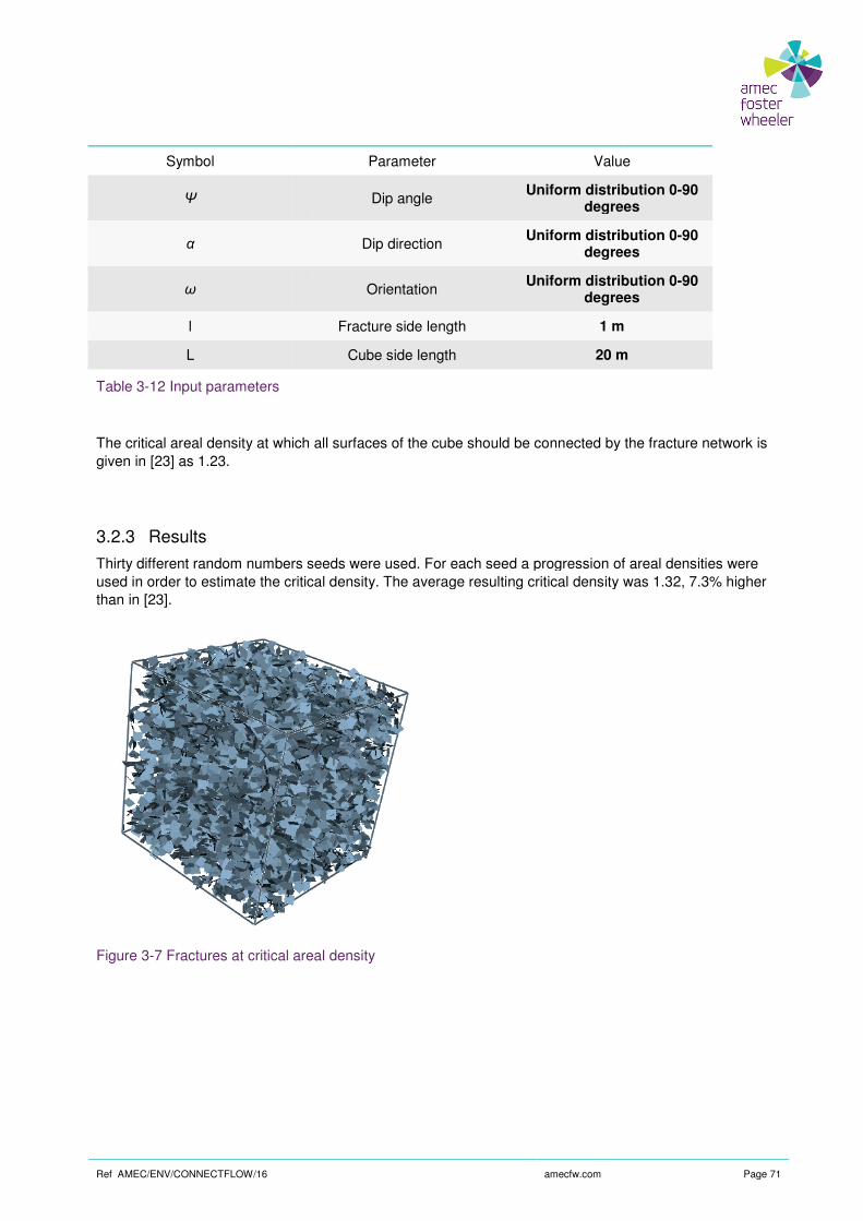
Ref AMEC/ENV/CONNECTFLOW/16
Symbol
Ψ
α
ω
l
L
Table 3-12 Input parameters
The critical areal density at which all surfaces of the cube should be connected by the fracture network is given in [23] as 1.23.
3.2.3 Results
Thirty different random numbers seeds were used. For each seed a progression of areal densities were used in order to estimate the critical density. The average resulting critical density was 1.32, 7.3% higher than in [23].
Figure 3-7 Fractures at critical areal density
amecfw.com
Parameter Value
Dip angle Uniform distribution 0
degrees
Dip direction Uniform distribution 0
degrees
Orientation Uniform distribution 0
degrees
Fracture side length 1 m
Cube side length 20 m
The critical areal density at which all surfaces of the cube should be connected by the fracture network is
seeds were used. For each seed a progression of areal densities were used in order to estimate the critical density. The average resulting critical density was 1.32, 7.3% higher
Fractures at critical areal density
Page 71
Value
Uniform distribution 0-90 degrees
Uniform distribution 0-90 degrees
Uniform distribution 0-90 degrees
1 m
20 m
The critical areal density at which all surfaces of the cube should be connected by the fracture network is
seeds were used. For each seed a progression of areal densities were used in order to estimate the critical density. The average resulting critical density was 1.32, 7.3% higher

Ref AMEC/ENV/CONNECTFLOW/16
3.3 3D Fracture Connectivity with a Power Law Size Distribution
3.3.1 Overview
This case considers the connectivity of random fractures within a cube, where the fracture lengths follow a power law distribution. The solution is taken from [
3.3.2 Problem Definition
The modelled domain is a cube for a range of increasing sizes. This is square fractures with side length corresponding to a truncated power law.
Symbol
Ψ
α
ω
a
L
Table 3-13 Input parameters
When the exponent is less than 3 the critical fracture density varies with domain size and the connectivity is dominated by the larger fractures. This is illustrated in
For large values of the exponent the connectivity of the smaller fractures dominates and the critical density does not vary with domain size for sufficiently large domains. This is similar
3.3.3 Results
A comparison of the dependence of the critical density on domain size is shown in reference data is taken from [23].
The results from ConnectFlow show good agreement, particularly in terms of thediscussed in [23], varies significantly with the exponent
amecfw.com
3D Fracture Connectivity with a Power Law Size Distribution
This case considers the connectivity of random fractures within a cube, where the fracture lengths follow a power law distribution. The solution is taken from [24].
The modelled domain is a cube for a range of increasing sizes. This is filled with randomly generated square fractures with side length corresponding to a truncated power law.
Parameter Value
Dip angle Uniform distribution 0
degrees
Dip direction Uniform distribution 0
degrees
Orientation Uniform distribution 0
degrees
Exponent in power law 2.5
Cube side length 5 - 300 m
When the exponent is less than 3 the critical fracture density varies with domain size and the connectivity is dominated by the larger fractures. This is illustrated in Figure 3-9.
For large values of the exponent the connectivity of the smaller fractures dominates and the critical density does not vary with domain size for sufficiently large domains. This is similar to case
A comparison of the dependence of the critical density on domain size is shown in
The results from ConnectFlow show good agreement, particularly in terms of the slope which, as ], varies significantly with the exponent a.
Page 72
3D Fracture Connectivity with a Power Law Size Distribution
This case considers the connectivity of random fractures within a cube, where the fracture lengths follow a
filled with randomly generated
Value
Uniform distribution 0-90 degrees
Uniform distribution 0-90 degrees
distribution 0-90 degrees
300 m
When the exponent is less than 3 the critical fracture density varies with domain size and the connectivity
For large values of the exponent the connectivity of the smaller fractures dominates and the critical density to case 3.1.
A comparison of the dependence of the critical density on domain size is shown in Figure 3-8. The
slope which, as

Ref AMEC/ENV/CONNECTFLOW/16
Figure 3-8 Critical fracture density variation with domain size
1.00E-04 1.00E-03
Fracture Density
Do
main
Sid
e L
en
gth
amecfw.com
ty variation with domain size
1
10
100
1000
1.00E-02 1.00E-01 1.00E+00
Fracture Density
ConnectFlow
Reference Data
Page 73
ConnectFlow
Reference Data
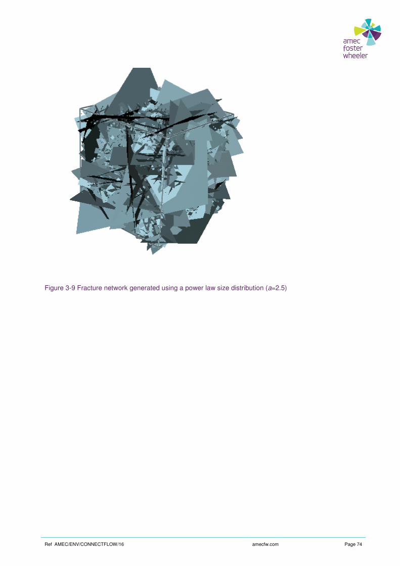
Ref AMEC/ENV/CONNECTFLOW/16
Figure 3-9 Fracture network generated using a power law size distribution (
amecfw.com
Fracture network generated using a power law size distribution (a=2.5)
Page 74

Ref AMEC/ENV/CONNECTFLOW/16
3.4 Upscaling from DFN to CPM
3.4.1 Overview
This case is taken from the DECOVALEX Task C [m region of fractured rock, generated from fracture mapping data from Sellafield UK.
The fracture set consists of 7797 fractures, with lengths varying from 0.5 to >30 m, and apertures varying from 1 to 200 microns.
The upscaled permeabilties are then used in a CPM calculation and the mass flows are compared.
3.4.2 Problem Definition
The modelled domain consists of a 20 m x 20 m x 1 m region with an applied horizontal pressure gradient of 1.0E4 Pa/m, as illustrated in Figure
Figure 3-10 Schematic of problem definition
The fracture distribution is shown in
Symbol
ρ
µ
amecfw.com
Upscaling from DFN to CPM
This case is taken from the DECOVALEX Task C [25] and calculates the permeability through a 20m region of fractured rock, generated from fracture mapping data from Sellafield UK.
The fracture set consists of 7797 fractures, with lengths varying from 0.5 to >30 m, and apertures varying
The upscaled permeabilties are then used in a CPM calculation and the mass flows are compared.
The modelled domain consists of a 20 m x 20 m x 1 m region with an applied horizontal pressure gradient Figure 3-10.
Schematic of problem definition
The fracture distribution is shown in Figure 3-11 and the input parameters in Table
Parameter Value
Density 1000 kg/m
Viscosity 1.0E-3 Ns/m
Page 75
calculates the permeability through a 20 m x 20 m region of fractured rock, generated from fracture mapping data from Sellafield UK.
The fracture set consists of 7797 fractures, with lengths varying from 0.5 to >30 m, and apertures varying
The upscaled permeabilties are then used in a CPM calculation and the mass flows are compared.
The modelled domain consists of a 20 m x 20 m x 1 m region with an applied horizontal pressure gradient
Table 3-14.
Value
1000 kg/m3
3 Ns/m2

Ref AMEC/ENV/CONNECTFLOW/16
Table 3-14 Input parameters
Figure 3-11 Fractured Rock
The DFN permeabilities are calculated on a regular grid of cells and the CPM calculation uses a regular grid of the same resolution. The finest grid resolution tested was 400x400 cells.
3.4.3 Variations
3.4.3.1 Cellular Model Calculation
The DFN region is overlayed with a
amecfw.com
permeabilities are calculated on a regular grid of cells and the CPM calculation uses a regular grid of the same resolution. The finest grid resolution tested was 400x400 cells.
Cellular Model Calculation
The DFN region is overlayed with a grid of cells of the required resolution.
Page 76
permeabilities are calculated on a regular grid of cells and the CPM calculation uses a regular

Ref AMEC/ENV/CONNECTFLOW/16
3.4.3.2 Cellular Model with Guard Zone
Each cell is stretched by a factor 3 in the x and z directions and then the middle section is used to export permeabilities for the area of interest. This helps improve accuracy wherthan one of the cells sides.
3.4.3.3 Regional Model Calculation
The DFN model region is used to define the grid of cells.
3.4.4 Results
The overall flow through the left hand boundary x=from [25] and the upscaled CPM results (with guard zone). The CPM result is 3% larger than the TUL result.
Approach
TUL
ConnectFlow DFN
ConnectFlow CPM (400 x 400 upscaling)
DFN and CPM Results without guard zones agreed to within 6%, whether calculated through region elements or through cellular model calculation.
The distribution of outflow at x = -10 m is compared between DFN and CPM models in range of upscaling resolutions. The data is averaged over 1 m intervals in order to better compare the bulk profile. Flow orthogonal to the pressure gradient at the outflow boundary z =
amecfw.com
Cellular Model with Guard Zone
Each cell is stretched by a factor 3 in the x and z directions and then the middle section is used to export permeabilities for the area of interest. This helps improve accuracy where single fractures intersect more
Regional Model Calculation
The DFN model region is used to define the grid of cells.
The overall flow through the left hand boundary x=-10 is compared against the stress free TUL resu] and the upscaled CPM results (with guard zone). The CPM result is 3% larger than the TUL
Flow X=-10
9.40E-5 m3/s
9.67E-5 m3/s
ConnectFlow CPM (400 x 400 upscaling) 9.71E-5 m3/s
DFN and CPM Results without guard zones agreed to within 6%, whether calculated through region elements or through cellular model calculation.
10 m is compared between DFN and CPM models in range of upscaling resolutions. The data is averaged over 1 m intervals in order to better compare the bulk profile. Flow orthogonal to the pressure gradient at the outflow boundary z = 10 m is shown in
Page 77
Each cell is stretched by a factor 3 in the x and z directions and then the middle section is used to export e single fractures intersect more
10 is compared against the stress free TUL results ] and the upscaled CPM results (with guard zone). The CPM result is 3% larger than the TUL
DFN and CPM Results without guard zones agreed to within 6%, whether calculated through region
10 m is compared between DFN and CPM models in Figure 3-12 for a range of upscaling resolutions. The data is averaged over 1 m intervals in order to better compare the bulk
10 m is shown in Figure 3-13.
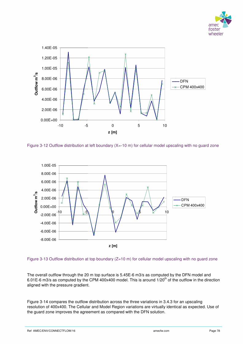
Ref AMEC/ENV/CONNECTFLOW/16
Figure 3-12 Outflow distribution at left boundary (X=
Figure 3-13 Outflow distribution at top boundary (Z=10 m) for cellular model upscaling with no guard zone
The overall outflow through the 20 m top surface is 5.45E6.01E-6 m3/s as computed by the CPM 400x400 model. This is around 1/20aligned with the pressure gradient.
Figure 3-14 compares the outflow distribution across the three variations in resolution of 400x400. The Cellular and Model Region variationthe guard zone improves the agreement as compared with the DFN solution.
0.00E+00
2.00E-06
4.00E-06
6.00E-06
8.00E-06
1.00E-05
1.20E-05
1.40E-05
-10 -5
Ou
tflo
w m
3/s
-8.00E-06
-6.00E-06
-4.00E-06
-2.00E-06
0.00E+00
2.00E-06
4.00E-06
6.00E-06
8.00E-06
1.00E-05
-10 -5Ou
tflo
w m
3/s
amecfw.com
Outflow distribution at left boundary (X=-10 m) for cellular model upscaling with no guard zone
Outflow distribution at top boundary (Z=10 m) for cellular model upscaling with no guard zone
The overall outflow through the 20 m top surface is 5.45E-6 m3/s as computed by the DFN model and 6 m3/s as computed by the CPM 400x400 model. This is around 1/20th of the outflow in the direction
aligned with the pressure gradient.
compares the outflow distribution across the three variations in 3.4.3 for an upscaling resolution of 400x400. The Cellular and Model Region variations are virtually identical as expected. Use of the guard zone improves the agreement as compared with the DFN solution.
-5 0 5 10
z [m]
0 5 10
z [m]
Page 78
aling with no guard zone
Outflow distribution at top boundary (Z=10 m) for cellular model upscaling with no guard zone
uted by the DFN model and of the outflow in the direction
for an upscaling s are virtually identical as expected. Use of
DFN
CPM 400x400
DFN
CPM 400x400

Ref AMEC/ENV/CONNECTFLOW/16
Figure 3-14 Comparison of outflows at left boundary (X=
0.00E+00
2.00E-06
4.00E-06
6.00E-06
8.00E-06
1.00E-05
1.20E-05
1.40E-05
-10 -5
Ou
tflo
w m
3/s
amecfw.com
Comparison of outflows at left boundary (X=-10m) using a CPM resolution of
-5 0 5 10
z [m]
Page 79
10m) using a CPM resolution of 400x400
DFN
Cellular
Region
Guard Zone

Ref AMEC/ENV/CONNECTFLOW/16
3.5 Radial Steady State Flow
3.5.1 Overview
This case models steady groundwater flow in a 2D disk where water is removed from the centre at a constant rate and the outer disk boundary is maintained at a constant head.
The example has a simple analytical
3.5.2 Problem Definition
This case is the DFN equivalent of
Figure 3-15 Schematic of problem definition
For a fracture, the aperture, e, is related to the hydraulic conductivity,
g
Ke
ρ
µ12=
The values in Table 3-15 have scaled Q from 1.0E
A 5 degree sector of the disk is modelled and is tessellated using 100 single fractures along its length. As these fractures are not rectangular, ConFigure 3-16.
amecfw.com
Radial Steady State Flow
This case models steady groundwater flow in a 2D disk where water is removed from the centre at a constant rate and the outer disk boundary is maintained at a constant head.
The example has a simple analytical solution and can be used to test a range of modelling choices.
This case is the DFN equivalent of Case 2.1.
Schematic of problem definition
, is related to the hydraulic conductivity, K by
have scaled Q from 1.0E-7 in Case 2.1 to give an equivalent head distribution.
A 5 degree sector of the disk is modelled and is tessellated using 100 single fractures along its length. As these fractures are not rectangular, ConnectFlow breaks them up into right angle triangles as illustrated in
Page 80
This case models steady groundwater flow in a 2D disk where water is removed from the centre at a
solution and can be used to test a range of modelling choices.
to give an equivalent head distribution.
A 5 degree sector of the disk is modelled and is tessellated using 100 single fractures along its length. As nectFlow breaks them up into right angle triangles as illustrated in

Ref AMEC/ENV/CONNECTFLOW/16
Figure 3-16 Fractures in sector of
The fractures used model the circumference of the sector as a straight line. As a result the accuracy of the simulation increases as the angle of the sector decreases.
The outflow at the axis is modelled using a borehole with a specified flow rate worthogonal to the disk.
Symbol
h
Q
K
R
e
r
ρ
µ
g
Table 3-15 Input parameters
3.5.3 Results
The analytical solution is given by
)ln(2
)()(r
R
Kd
QRhrh
π−=
The results from ConnectFlow show good agreement with the analytical solution, as illustrated in 3-17.
amecfw.com
disk
The fractures used model the circumference of the sector as a straight line. As a result the accuracy of the angle of the sector decreases.
The outflow at the axis is modelled using a borehole with a specified flow rate which has direction
Parameter Value
Head at disk circumference 0 m
Outflow from disk 1.11E-14 m
Hydraulic Conductivity 1.0E-8 m/s
Radius of disk 2000 m
Aperture of fracture 1.11E-
Radial distance from axis 0-2000 m
Density 1000 kg/m
Viscosity 1.0E-3 Pa.s
Gravity 9.8 m/s
The analytical solution is given by
The results from ConnectFlow show good agreement with the analytical solution, as illustrated in
Page 81
The fractures used model the circumference of the sector as a straight line. As a result the accuracy of the
hich has direction
Value
0 m
14 m3/s
8 m/s
2000 m
-7 m
2000 m
1000 kg/m3
3 Pa.s
9.8 m/s2
The results from ConnectFlow show good agreement with the analytical solution, as illustrated in Figure

Ref AMEC/ENV/CONNECTFLOW/16
Figure 3-17 Variation of head with distance from the axis with an outflow modelled with a borehole
-8
-7
-6
-5
-4
-3
-2
-1
0
0 500
Radius [m]
He
ad
[m
]
amecfw.com
Variation of head with distance from the axis with an outflow modelled with a borehole
1000 1500 2000
Radius [m]
ConnectFlow
Analytical Solution
Page 82
Variation of head with distance from the axis with an outflow modelled with a borehole
ConnectFlow
Analytical Solution

Ref AMEC/ENV/CONNECTFLOW/16
3.6 Three Fracture Intersections
3.6.1 Overview
This case models steady groundwater flow and particle tracking in a simple two dimensional fracture network.
3.6.2 Problem Definition
The problem is a variant of test C1 from DarcyTools [region as shown in Figure 3-18.
Figure 3-18 Three fracture intersections
A 3x3 system of linear equations is derived by applying intersections. This is used to calculate the heads at a, b and c and hence the flow rates in each fracture segment.
The fracture geometry used for this test is defined in
X Start Y Start
0
0
0
Table 3-16 Fracture locations
amecfw.com
Three Fracture Intersections
This case models steady groundwater flow and particle tracking in a simple two dimensional fracture
The problem is a variant of test C1 from DarcyTools [26]. Three fractures are placed in a rectangular
Three fracture intersections
A 3x3 system of linear equations is derived by applying mass conservation at the three fracture intersections. This is used to calculate the heads at a, b and c and hence the flow rates in each fracture
The fracture geometry used for this test is defined in Table 3-16.
Y Start X End Y End
2 12
3 12
5 12
Page 83
This case models steady groundwater flow and particle tracking in a simple two dimensional fracture
]. Three fractures are placed in a rectangular
mass conservation at the three fracture intersections. This is used to calculate the heads at a, b and c and hence the flow rates in each fracture
Y End
5
3
2

Ref AMEC/ENV/CONNECTFLOW/16
3.6.3 Variations
3.6.3.1 Symmetric
For the symmetric case, the fracture analytical flow field where the flow rates along each fracture are almost identical.
3.6.3.2 Non-symmetric
In the non-symmetric case, the fracture apertures are set to 1.0Esection bc, 2.0E-4 m for section ac and 4.0Ethrough ab is removed as shown in
Figure 3-19 Non symmetric fractures
This arrangement means that the flow at b splits, with some of it moving to c and then a, and the rest moving directly towards the left hand boundary.
The particle tracking is tested by releasing 10000 particles at the h=1 surface, with the fraction of particles in each fracture distributed in proportion to the analytical inflow rate.
The proportion of particles leaving the geometry at Y=2, 3 and 5 analytically predicted outflow rates.
Y Analytical inflow distribution
2
3
5
Table 3-17 Analytical inflow/outflow
amecfw.com
For the symmetric case, the fracture aperture is set to 1.0E-4 m for all three fractures. This gives an analytical flow field where the flow rates along each fracture are almost identical.
symmetric case, the fracture apertures are set to 1.0E-4 m for the fracture pa4 m for section ac and 4.0E-4 m for section ab. In addition, the section of fracture passing
through ab is removed as shown in Figure 3-19.
Non symmetric fractures
This arrangement means that the flow at b splits, with some of it moving to c and then a, and the rest moving directly towards the left hand boundary.
The particle tracking is tested by releasing 10000 particles at the h=1 surface, with the fraction of particles in each fracture distributed in proportion to the analytical inflow rate.
The proportion of particles leaving the geometry at Y=2, 3 and 5 should correspond to the ratio of the analytically predicted outflow rates.
Analytical inflow distribution at X=12
Analytical outflow distribution at X=0
7.9% 77.3%
64.9% 10.0%
27.2% 12.7%
Analytical inflow/outflow
Page 84
4 m for all three fractures. This gives an
4 m for the fracture passing through 4 m for section ab. In addition, the section of fracture passing
This arrangement means that the flow at b splits, with some of it moving to c and then a, and the rest
The particle tracking is tested by releasing 10000 particles at the h=1 surface, with the fraction of particles
should correspond to the ratio of the

Ref AMEC/ENV/CONNECTFLOW/16
For this test, the APPROXIMATE PARTICLE TRACKING inflow to outflow and backward tracking to track from outflow to inflow.
3.6.3.3 Symmetric – Exact Particle tracking
This test is identical to the symmetric case, but using the of approximate particle tracking.
The proportion of particles leaving the geometry at Y=2, 3 and 5 should correspond to the ratio of the analytically predicted outflow rates, i.e. it should be the same in all three locations.
3.6.4 Results
3.6.4.1 Symmetric
The predicted results for head are within 1% of the analytical values.
Intersection ConnectFlow
a 0.333
b 0.496
c 0.667
Table 3-18 Heads at fracture intersections
3.6.4.2 Non Symmetric
The ConnectFlow head distribution for this case is shown in and particle flows are within 5% of the analytical values.
Figure 3-20 Head distribution
amecfw.com
APPROXIMATE PARTICLE TRACKING model is used, with forward tracking to track from inflow to outflow and backward tracking to track from outflow to inflow.
Exact Particle tracking
This test is identical to the symmetric case, but using the EXACT PARTICLE TRACKING
The proportion of particles leaving the geometry at Y=2, 3 and 5 should correspond to the ratio of the ed outflow rates, i.e. it should be the same in all three locations.
re within 1% of the analytical values.
ConnectFlow Analytical % Error
0.333 0.333 0.19%
0.496 0.500 0.89%
0.667 0.667 0.10%
Heads at fracture intersections
The ConnectFlow head distribution for this case is shown in Figure 3-20. Predicted results for the head and particle flows are within 5% of the analytical values.
Page 85
model is used, with forward tracking to track from
EXACT PARTICLE TRACKING method instead
The proportion of particles leaving the geometry at Y=2, 3 and 5 should correspond to the ratio of the
% Error
0.19%
0.89%
0.10%
. Predicted results for the head

Ref AMEC/ENV/CONNECTFLOW/16
Intersection ConnectFlow
a 0.062
b 0.937
c 0.599
Table 3-19 Heads at fracture intersections
Y at Exit ConnectFlow
2 7.4%
3 65.6%
5 27.0%
Table 3-20 Particle flow rates (backwards)
Y at Exit ConnectFlow
2 77.6%
3 9.5%
5 12.9%
Table 3-21 Particle flow rates (forwards)
3.6.4.3 Symmetric – Exact Particle tracking
The predicted proportions of particles leaving the model at each location are within 1% of the analytical values.
Y at Exit ConnectFlow
2 33.1%
3 33.8%
5 33.1%
Table 3-22 Proportions of particles at each outflow point
amecfw.com
ConnectFlow Analytical % Error
0.061 1.49%
0.968 3.23%
0.600 0.15%
Heads at fracture intersections
ConnectFlow Analytical Error
7.4% 7.9% 0.5%
65.6% 65.0% 0.6%
27.0% 27.2% 0.2%
Particle flow rates (backwards)
ConnectFlow Analytical Error
77.6% 77.3% 0.3%
9.5% 10.0% 0.5%
12.9% 12.7% 0.2%
Particle flow rates (forwards)
Exact Particle tracking
of particles leaving the model at each location are within 1% of the analytical
ConnectFlow Analytical % Error
33.1% 33.3% 0.2%
33.8% 33.3% 0.5%
33.1% 33.3% 0.2%
Proportions of particles at each outflow point using exact particle tracking
Page 86
% Error
1.49%
3.23%
0.15%
Error
0.5%
0.6%
0.2%
Error
0.3%
0.5%
0.2%
of particles leaving the model at each location are within 1% of the analytical
% Error
0.2%
0.5%
0.2%
using exact particle tracking

Ref AMEC/ENV/CONNECTFLOW/16
3.7 Steady Flow in Fractured Rock
3.7.1 Overview
The example is taken from Level 1 of the international HYDROCOIN project for verification of groundwater flow codes [27] and is the same problem as CPM C
It models steady state flow in a twoinclined fractures which intersect one another at depth, and have a higher permeabilsurrounding rock.
The topography has been made simple so that it consists of two valleys located where the fracture zones meet the surface. To simplify the problem definition, the shape of the surface is described by straight lines. Although the surface topography is symmetric, the flow is influenced by the asymmetry of the fracture zones.
This problem is based on an idealized version of the hydrogeological conditions encountered
at a potential site for a deep repository in Swedish bedrock. A
model of this was made in a separate study [
3.7.2 Problem Definition
Figure 3-21 depicts the modelled domain.
Figure 3-21 Fractured rock
amecfw.com
Steady Flow in Fractured Rock
The example is taken from Level 1 of the international HYDROCOIN project for verification of groundwater and is the same problem as CPM Case 2.2.
It models steady state flow in a two-dimensional vertical slice of fractured rock. The rock contains two inclined fractures which intersect one another at depth, and have a higher permeabil
The topography has been made simple so that it consists of two valleys located where the fracture zones meet the surface. To simplify the problem definition, the shape of the surface is described by straight lines.
the surface topography is symmetric, the flow is influenced by the asymmetry of the fracture
This problem is based on an idealized version of the hydrogeological conditions encountered
at a potential site for a deep repository in Swedish bedrock. A detailed three-dimensional
model of this was made in a separate study [28].
depicts the modelled domain.
Page 87
The example is taken from Level 1 of the international HYDROCOIN project for verification of groundwater
dimensional vertical slice of fractured rock. The rock contains two inclined fractures which intersect one another at depth, and have a higher permeability than the
The topography has been made simple so that it consists of two valleys located where the fracture zones meet the surface. To simplify the problem definition, the shape of the surface is described by straight lines.
the surface topography is symmetric, the flow is influenced by the asymmetry of the fracture
This problem is based on an idealized version of the hydrogeological conditions encountered
dimensional

Ref AMEC/ENV/CONNECTFLOW/16
Symbol
Kr Hydraulic conductivity of rock
Krf Hydraulic conductivity of CPM
e1
e2
Table 3-23 Input parameters
The fracture apertures have been derived to match the transmissivities of the fracture regions in case 2.2.2. For the DFN model, the transmissivity is proportional to aperture cubed and for the CPM model it is proportional to the cross sectional thickness of the region representing the fracture.
The rock is modelled using an arrayperspective to make it easier to visualise.
Figure 3-22 Modelled fractures
amecfw.com
Parameter Value
Hydraulic conductivity of rock 1.0E-8 m/s
Hydraulic conductivity of CPM fractured region
1.0E-6 m/s
Thickness of fracture F1 2.053E-
Thickness of fracture F2 2.620E-
The fracture apertures have been derived to match the transmissivities of the fracture regions in case . For the DFN model, the transmissivity is proportional to aperture cubed and for the CPM model it is
proportional to the cross sectional thickness of the region representing the fracture.
The rock is modelled using an array of fractures as shown in Figure 3-22. The figure is drawn in perspective to make it easier to visualise.
Page 88
Value
8 m/s
6 m/s
-4 m
-4 m
The fracture apertures have been derived to match the transmissivities of the fracture regions in case . For the DFN model, the transmissivity is proportional to aperture cubed and for the CPM model it is
proportional to the cross sectional thickness of the region representing the fracture.
. The figure is drawn in

Ref AMEC/ENV/CONNECTFLOW/16
3.7.3 Variations
3.7.3.1 IFZ Rock Matrix
In this variant, the rock matrix is modelled using a two dimensional grid of fractures that are read in as an Implict Fracture Zone (IFZ) file.
3.7.3.2 Matrix Lattice Option
In this variant, the rock matrix is modelled using a three dimensional grid of fractures generated by the command GENERATE MATRIX LATTICE. approximately twice as wide as that set manually in t
3.7.3.3 Current Value
In this variant, a subset of the domain is modelled, x = 100 to 1500 m and y = illustrated in Figure 3-23.The boundary pressure is taken from the CPM solution the >>CURRENT VALUE boundary condition option. The rock matrix is modelled approach as in 3.7.3.1.
Figure 3-23 Current Value
3.7.4 Results
The results presented here comparagreement with the HYDROCOIN study.
amecfw.com
In this variant, the rock matrix is modelled using a two dimensional grid of fractures that are read in as an
In this variant, the rock matrix is modelled using a three dimensional grid of fractures generated by the GENERATE MATRIX LATTICE. In this case, the fracture widths are set automatically and are
approximately twice as wide as that set manually in the IFZ Rock Matrix variant.
In this variant, a subset of the domain is modelled, x = 100 to 1500 m and y = -300 to .The boundary pressure is taken from the CPM solution 2.2.3.1boundary condition option. The rock matrix is modelled using the same IFZ
The results presented here compare the head profile at a height of y=-200 m and show excellent agreement with the HYDROCOIN study.
Page 89
In this variant, the rock matrix is modelled using a two dimensional grid of fractures that are read in as an
In this variant, the rock matrix is modelled using a three dimensional grid of fractures generated by the In this case, the fracture widths are set automatically and are
300 to -100 m. This is 2.2.3.1 and applied using using the same IFZ
200 m and show excellent

Ref AMEC/ENV/CONNECTFLOW/16
Figure 3-24 Head at height -200 m (IFZ Rock Matrix)
Figure 3-25 Head at height -200 m (Matrix Lattice)
100
105
110
115
120
125
0 400
Distance [m]
Head
[m
]
100
105
110
115
120
125
0 400
Distance [m]
Head
[m
]
amecfw.com
200 m (IFZ Rock Matrix)
200 m (Matrix Lattice)
800 1200 1600
Distance [m]
ConnectFlow
Hydrocoin
800 1200 1600
Distance [m]
ConnectFlow
Hydrocoin
Page 90
ConnectFlow
Hydrocoin
ConnectFlow
Hydrocoin

Ref AMEC/ENV/CONNECTFLOW/16
Figure 3-26 Head at height -200 m (Current Value)
In addition, the ConnectFlow results were compared against the Feftra base case results [differences in head between the two codes being less than 0.5% for the IFZ Rock Matrix and Reduced Domain variants and less than 1% for the Matrix Lat
The latter is marginally less accurate due to the increased permeability contribution of the wider rock matrix fractures. This was checked by making the fractures in the IFZ Rock Matrix variant deliberately wider and the same trend was seen.
Figure 3-27 shows the head distribution through the fracture network.
100
105
110
115
120
125
0 400
Distance [m]
Head
[m
]
amecfw.com
200 m (Current Value)
In addition, the ConnectFlow results were compared against the Feftra base case results [differences in head between the two codes being less than 0.5% for the IFZ Rock Matrix and Reduced Domain variants and less than 1% for the Matrix Lattice.
The latter is marginally less accurate due to the increased permeability contribution of the wider rock matrix fractures. This was checked by making the fractures in the IFZ Rock Matrix variant deliberately wider and the same trend was seen.
shows the head distribution through the fracture network.
800 1200 1600
Distance [m]
ConnectFlow
Hydrocoin
Page 91
In addition, the ConnectFlow results were compared against the Feftra base case results [3], with the differences in head between the two codes being less than 0.5% for the IFZ Rock Matrix and Reduced
The latter is marginally less accurate due to the increased permeability contribution of the wider rock matrix fractures. This was checked by making the fractures in the IFZ Rock Matrix variant deliberately
ConnectFlow
Hydrocoin

Ref AMEC/ENV/CONNECTFLOW/16
Figure 3-27 Fractures coloured by head (IFZ Ro
amecfw.com
Fractures coloured by head (IFZ Rock Matrix)
Page 92

Ref AMEC/ENV/CONNECTFLOW/16
3.8 Henry’s Salt Transport
3.8.1 Overview
This case considers salt water intrusion into a vertical slice of an isotropic homogeneous confined aquifer.
The variant modelled is a modified version of the original Henry‘s test case, as recommended in [modified case halves the fresh water inflow rate, which increases the sensitivity of the solution to the variation in density.
This case is the DFN equivalent of C
3.8.2 Problem Definition
A schematic of the test case is shown in
Figure 3-28 Schematic illustration of the Henry test case
amecfw.com
Henry’s Salt Transport
This case considers salt water intrusion into a vertical slice of an isotropic homogeneous confined aquifer.
The variant modelled is a modified version of the original Henry‘s test case, as recommended in [modified case halves the fresh water inflow rate, which increases the sensitivity of the solution to the
nt of Case 2.8.
A schematic of the test case is shown in Figure 3-28 and the input parameters are given in
Schematic illustration of the Henry test case
Page 93
This case considers salt water intrusion into a vertical slice of an isotropic homogeneous confined aquifer.
The variant modelled is a modified version of the original Henry‘s test case, as recommended in [14]. The modified case halves the fresh water inflow rate, which increases the sensitivity of the solution to the
and the input parameters are given in Table 3-24.

Ref AMEC/ENV/CONNECTFLOW/16
Symbol
K Hydraulic conductivity of rock
D
Q
0ρ
maxρ
Lα
Tα
φ
Table 3-24 Input parameters
The domain is represented by a single fracture tessellated into 0.025 m square thickness is set to 1.8516E-4 m in order to generate the desired hydraulic conductivity of 1.0E
The fracture has a porosity of 1.0 rather than 0.35 in [in order to account for this and to get the appropriate velocity field.
3.8.3 Variations
3.8.3.1 Interpolated Density
The density is interpolated from the CPM solution of test Ccalculation.
3.8.3.2 Salt Transport
The salt transport is modelled and the density calculated from the salinity.
3.8.4 Results
3.8.4.1 Interpolated Density
The interpolated density field used is shown in
amecfw.com
Parameter Value
Hydraulic conductivity of rock 1.0E-2 m/s
Coefficient of molecular diffusion
1.886E-5 m
Freshwater inflow per unit depth
9.43E-5 m
Reference density 998 kg/m
Saltwater density 1023 kg/m
Longitudinal dispersivity 0 m
Transverse dispersivity 0 m
Porosity 1
The domain is represented by a single fracture tessellated into 0.025 m square sub4 m in order to generate the desired hydraulic conductivity of 1.0E
The fracture has a porosity of 1.0 rather than 0.35 in [14]. The inflow rate is increased by a factor of 1/0.35 in order to account for this and to get the appropriate velocity field.
from the CPM solution of test Case 2.8 and kept fixed throughout the
The salt transport is modelled and the density calculated from the salinity.
The interpolated density field used is shown in Figure 3-29.
Page 94
Value
2 m/s
5 m2/s
5 m2/s
998 kg/m3
1023 kg/m3
0 m
0 m
sub-fractures. The fracture 4 m in order to generate the desired hydraulic conductivity of 1.0E-2 m/s.
]. The inflow rate is increased by a factor of 1/0.35
and kept fixed throughout the

Ref AMEC/ENV/CONNECTFLOW/16
Figure 3-29 Interpolated density
The pressure field is compared against the reference CPM solution, the latter having been separately checked against the analytical solution via the salt concentration.
Plots of the two pressure fields are shown in within 5%.
amecfw.com
field is compared against the reference CPM solution, the latter having been separately checked against the analytical solution via the salt concentration.
Plots of the two pressure fields are shown in Figure 3-30 and Figure 3-31. The pressure fields agree to
Page 95
field is compared against the reference CPM solution, the latter having been separately
. The pressure fields agree to

Ref AMEC/ENV/CONNECTFLOW/16
Figure 3-30 DFN residual pressure
Figure 3-31 CPM Residual pressure
3.8.4.2 Salt Transport
This test case has an analytical solution, represented by an infinite double Fourier series. A truncated form of the series gives a non linear system which can then be iteratively solved. Results from this process are
amecfw.com
DFN residual pressure
M Residual pressure
This test case has an analytical solution, represented by an infinite double Fourier series. A truncated form of the series gives a non linear system which can then be iteratively solved. Results from this process are
Page 96
This test case has an analytical solution, represented by an infinite double Fourier series. A truncated form of the series gives a non linear system which can then be iteratively solved. Results from this process are

Ref AMEC/ENV/CONNECTFLOW/16
reported in [14] and these are used for comparisons in is less than 2%.
Figure 3-32 Non-dimensional concentration of salinity
0.00
0.10
0.20
0.30
0.40
0.50
0.60
0.70
0.80
0.90
1.00
0.00 0.20 0.40 0.60
z [
m]
ConnectFlow 25%
Semi analytical 25%
ConnectFlow 50%
Semi analytical 50%
ConnectFlow 75%
Semi analytical 75%
amecfw.com
] and these are used for comparisons in Figure 3-32. The maximum error in contour location
dimensional concentration of salinity
0.60 0.80 1.00 1.20 1.40 1.60 1.80
X [m]
ConnectFlow 25%
Semi analytical 25%
ConnectFlow 50%
Semi analytical 50%
ConnectFlow 75%
Semi analytical 75%
Page 97
mum error in contour location
2.00

Ref AMEC/ENV/CONNECTFLOW/16
3.9 Salt Transport
3.9.1 Overview
This case considers 1D transport of
3.9.2 Problem Definition
A schematic of the test case is shown in
Figure 3-33 A schematic of the single fracture test case using an outflow (zero dispersive flux) boundary condition. The single fracture is 2 m wide and 1 m high, tessellated to a length of 0.025
Parameter
Fracture transmissivity
Freshwater inflow per unit depth
Reference density
Saltwater density
Salinity dispersion
Table 3-25 Input parameters
The domain is represented by a single fracture tessellated into 0.025 m square subtransmissivity is set to 5.3E-6 m2/s. The is introduced through its bottom edge. The boundary conditions are zero dispersive flux and a constant pressure on the top surface, and no flow on the sides of the fracture.
amecfw.com
This case considers 1D transport of salt water due to a pressure gradient.
A schematic of the test case is shown in Figure 3-33 and the input parameters are given in
A schematic of the single fracture test case using an outflow (zero dispersive flux) boundary ingle fracture is 2 m wide and 1 m high, tessellated to a length of 0.025
Value
5.3E-6 m2/s
3.49E-8 m3/s
1000 kg/m3
1025 kg/m3
1.886E-5 m2/s
The domain is represented by a single fracture tessellated into 0.025 m square sub/s. The fracture initially contains fresh water throughout, and saline water
is introduced through its bottom edge. The boundary conditions are zero dispersive flux and a constant pressure on the top surface, and no flow on the sides of the fracture.
Page 98
and the input parameters are given in Table 3-25.
A schematic of the single fracture test case using an outflow (zero dispersive flux) boundary ingle fracture is 2 m wide and 1 m high, tessellated to a length of 0.025 m.
The domain is represented by a single fracture tessellated into 0.025 m square sub-fractures. The fracture fracture initially contains fresh water throughout, and saline water
is introduced through its bottom edge. The boundary conditions are zero dispersive flux and a constant

Ref AMEC/ENV/CONNECTFLOW/16
3.9.3 Results
A steady state salt transport calculation was carried out, the anticipated solution being a constant salinity of 1.0 throughout the model. Results agreed with this solution to within 2%.
3.10 Salt Upconing
3.10.1 Overview
This case considers the upconing of salt water ia 2D case). To verify the case, equivalent CPM and DFN calculations were carried out to ensure that they produced consistent results.
3.10.2 Problem Definition
A schematic of the test case is shown in
Figure 3-34 Model of a vertical crossand 4 m high.
amecfw.com
teady state salt transport calculation was carried out, the anticipated solution being a constant salinity of 1.0 throughout the model. Results agreed with this solution to within 2%.
This case considers the upconing of salt water into a tunnel in the centre of a thin 3D model (representing a 2D case). To verify the case, equivalent CPM and DFN calculations were carried out to ensure that they
A schematic of the test case is shown in Figure 3-34 and the input parameters are given in
Model of a vertical cross-section, 800 m high and 1200 m wide. The open tunnel is 3
Page 99
teady state salt transport calculation was carried out, the anticipated solution being a constant salinity
nto a tunnel in the centre of a thin 3D model (representing a 2D case). To verify the case, equivalent CPM and DFN calculations were carried out to ensure that they
and the input parameters are given in Table 3-26.
m wide. The open tunnel is 3 m wide

Ref AMEC/ENV/CONNECTFLOW/16
Symbol
K Hydraulic conductivity (CPM)
φ
D Coefficient of molecular
0ρ
maxρ
Lα Longitudinal
Tα Transverse dispersion length
Table 3-26 Salt transport input parameters
To ensure that the same parameters are used in both cases, the conductivities are transmissivities to be input to the DFN. The tunnel is represented by a void in the model, with a depth range of 400 m to 404 m in the centre of the model.
There is zero dispersive flux at the tunnel and a residual pressure of The specified initial condition is a depthof:
+−
−≥>−=
−
−
)800(10983.11
400010172.5
3
4
z
zzs
The salinity profile used as the boundary condition uses the same values.
In order to achieve convergence, the model requires a parameterstep has D = 1.0E-4 m2/s, and the result is used as the initial condition for a step with D
amecfw.com
Parameter Value
Hydraulic conductivity (CPM) Equivalent hydraulic conductivity (DFN)
=
−
−
−
−
/108.1
/102.1
/106.1
/109.3
11
10
9
8
m
m
m
m
K
Porosity
=
−
−
−
−
1011.6
1015.1
1070.2
1090.7
6
5
5
5
ϕ
Coefficient of molecular diffusion
1.0E
Reference density 998.217 kg/m
Saltwater density 1042 kg/m
Longitudinal dispersion length
Transverse dispersion length
Salt transport input parameters
To ensure that the same parameters are used in both cases, the conductivities are transmissivities to be input to the DFN. The tunnel is represented by a void in the model, with a depth range of 400 m to 404 m in the centre of the model.
There is zero dispersive flux at the tunnel and a residual pressure of -4.0E6 Pa (atmThe specified initial condition is a depth-dependent salinity, equivalent in both cases. This has a salinity
−≥>− .800400
,400
z
The salinity profile used as the boundary condition uses the same values.
convergence, the model requires a parameter-stepping technique be used: the first /s, and the result is used as the initial condition for a step with D
Page 100
Value
−≥>−
−≥>−
−≥>−
−≥>
.800400/
,400150/
,15050
,500/
zs
zs
zs
zs
−≥>−
−≥>−
−≥>−
−≥>
.800400
,400150
,15050
,500
z
z
z
z
1.0E-6 m2/s
998.217 kg/m3
1042 kg/m3
3 m
1 m
To ensure that the same parameters are used in both cases, the conductivities are converted to transmissivities to be input to the DFN. The tunnel is represented by a void in the model, with a depth
4.0E6 Pa (atmospheric pressure). dependent salinity, equivalent in both cases. This has a salinity
stepping technique be used: the first /s, and the result is used as the initial condition for a step with D = 1.0E-6 m2/s

Ref AMEC/ENV/CONNECTFLOW/16
3.10.3 Results
The results shown in Figure 3-35 (DFN) and upconing of salt into the tunnel as antici
Results for the model are taken in a central line from 405 m to 800 m depth at fivefrom just below the tunnel to the bottom of the model), as plotted in results agreed to within 10%, with the largest differences close to the tunnel.
Figure 3-35 DFN Salinity profile
amecfw.com
(DFN) and Figure 3-36 (CPM) are a good match and demonstrate upconing of salt into the tunnel as anticipated.
Results for the model are taken in a central line from 405 m to 800 m depth at five-from just below the tunnel to the bottom of the model), as plotted in Figure 3-37. The CPM and DFN results agreed to within 10%, with the largest differences close to the tunnel.
Page 101
(CPM) are a good match and demonstrate
-metre intervals (i.e. . The CPM and DFN

Ref AMEC/ENV/CONNECTFLOW/16
Figure 3-36 CPM Salinity profile
Figure 3-37 Difference between CPM and DFN results in the upconing case.
-800
-750
-700
-650
-600
-550
-500
-450
-400
0 0.1 0.2 0.3
De
pth
[m
]
DFN Result
CPM Result
amecfw.com
Difference between CPM and DFN results in the upconing case.
0.3 0.4 0.5 0.6 0.7 0.8
Salinity
Page 102
0.9 1

Ref AMEC/ENV/CONNECTFLOW/16
3.11 Grouting of a fracture
3.11.1 Overview
The grouting of the intersection of a single fracture and an external surface can be solved analytically and is used for verification of the implementation of a grouting model.
3.11.2 Problem definition
Grouting of fractures can be specified in a variety of manners. In this case a grois used. That is, the flow after applying the grout is reduced by a factor of 10. In terms of hydraulic aperture this means a reduction of aperture by a factor f,
f = (1-e)1/3 = 0.464.
The model is defined as follows.
The region is a simple rectangular region with the coordinates specified in
Top
Bottom
Left
Right
Front
Back
Table 3-27 Region coordinates for fracture
One ‘known’ fracture is added in the yz plane, connecting the top and bottom, with a width (w) of 2.0The height (h) is the distance between
The pressure boundary condition at the top is zero and at the bottom it is
where ρ is the fluid density (1000 kg/mparameter to specify an overpressure.
amecfw.com
Grouting of a fracture – surface intersection
ersection of a single fracture and an external surface can be solved analytically and is used for verification of the implementation of a grouting model.
Grouting of fractures can be specified in a variety of manners. In this case a grouting efficiency (e) of 90% is used. That is, the flow after applying the grout is reduced by a factor of 10. In terms of hydraulic aperture this means a reduction of aperture by a factor f,
egion is a simple rectangular region with the coordinates specified in Table 3-
(m)
0
-10
-5
5
-5
5
Region coordinates for fracture-surface intersection grouting
One ‘known’ fracture is added in the yz plane, connecting the top and bottom, with a width (w) of 2.0The height (h) is the distance between the intersections at the top and bottom surfaces, i.e. 10.0
The pressure boundary condition at the top is zero and at the bottom it is
P = ρ g (h – s),
is the fluid density (1000 kg/m3), g the gravitational acceleration (9.81 kg m/sparameter to specify an overpressure.
Page 103
ersection of a single fracture and an external surface can be solved analytically and
uting efficiency (e) of 90% is used. That is, the flow after applying the grout is reduced by a factor of 10. In terms of hydraulic aperture
-27.
One ‘known’ fracture is added in the yz plane, connecting the top and bottom, with a width (w) of 2.0 m. the intersections at the top and bottom surfaces, i.e. 10.0 m.
), g the gravitational acceleration (9.81 kg m/s2) and s is a

Ref AMEC/ENV/CONNECTFLOW/16
For this simple problem, the Darcy flow equation can be solved explicitly and the solution is:
or, with the pressures shown as above:
Q = T w s / h,
where T is the transmissivity of the fracture. The ungrouted transmissivity is taken to be 10grouted transmissivity will be a factor of 10 smaller.
The overpressure parameter is 2.0specified in terms of residual pressure, so the value at the bottom is 19620.0
3.11.3 Results
The results are presented in Table ungrouted flows out of the top surface .The second column is the result of a ConnectFlow calculation with the fracture untessellated and the last column is the same but with a tessellation length of 1.0leads to it being broken up into 20 tesselthe whole fracture is grouted.
Analytical
Ungrouted 4.000E
Grouted 4.000E
Table 3-28. Grouting results for fracture
3.12 Grouting of a fracture
3.12.1 Overview
Fracture-fracture intersections will only be grouted if one of the factures belongs trepresenting some physical features, such as a tunnel, shaft or deposition hole.
amecfw.com
For this simple problem, the Darcy flow equation can be solved explicitly and the solution is:
Q = -(T w / ρ g) (∆P - ρ g),
or, with the pressures shown as above:
f the fracture. The ungrouted transmissivity is taken to be 10grouted transmissivity will be a factor of 10 smaller.
The overpressure parameter is 2.0 m. Note that the pressure boundary condition in a DFN model is al pressure, so the value at the bottom is 19620.0 Pa.
Table 3-28. The first column has the analytical results for the grouted anungrouted flows out of the top surface .The second column is the result of a ConnectFlow calculation with the fracture untessellated and the last column is the same but with a tessellation length of 1.0leads to it being broken up into 20 tessellates. Note that a large penetration depth is used to assure that
Analytical Untessellated fracture Tessellated fracture
4.000E-5 m3/s 4.000E-5 m3/s 3.997E
4.000E-6 m3/s 4.000E-6 m3/s 3.997E
. Grouting results for fracture-surface intersection
Grouting of a fracture – fracture intersection
fracture intersections will only be grouted if one of the factures belongs to a set of fractures representing some physical features, such as a tunnel, shaft or deposition hole.
Page 104
For this simple problem, the Darcy flow equation can be solved explicitly and the solution is:
f the fracture. The ungrouted transmissivity is taken to be 10-4 m2/s. The
m. Note that the pressure boundary condition in a DFN model is
. The first column has the analytical results for the grouted and ungrouted flows out of the top surface .The second column is the result of a ConnectFlow calculation with the fracture untessellated and the last column is the same but with a tessellation length of 1.0 m, which
lates. Note that a large penetration depth is used to assure that
Tessellated fracture
3.997E-5 m3/s
3.997E-6 m3/s
o a set of fractures

Ref AMEC/ENV/CONNECTFLOW/16
3.12.2 Problem definition
The ‘feature’ is the horizontal fracture in the figure below. It is connected by a single fracture to the top surface and another to the bottom surface, as shown in
Figure 3-38. Fractures used for fracture
The model region is a simple rectangular volume with the coordinates specified in
Top
Bottom
Left
Right
Front
Back
Table 3-29. Region coordinates for fracture
amecfw.com
The ‘feature’ is the horizontal fracture in the figure below. It is connected by a single fracture to the top surface and another to the bottom surface, as shown in Figure 3-38.
. Fractures used for fracture-fracture intersection grouting
The model region is a simple rectangular volume with the coordinates specified in Table
(m)
0
-10
-5
5
-5
5
. Region coordinates for fracture-fracture intersection grouting
Page 105
The ‘feature’ is the horizontal fracture in the figure below. It is connected by a single fracture to the top
Table 3-29.

Ref AMEC/ENV/CONNECTFLOW/16
The Darcy flow equation for this system can be solved explicitly. The parameters used are indicated in the vertical slice in Figure 3-39.
Figure 3-39. Parameters used for fracturethe fractures
In terms of these z-coordinates (z), lengths betwe(T) the solution for the outflow at the top is:
Q = (P1 - P
where w is the common width of all fractures. With the following choices:
this reduces to
z1, pressure P
La, Ta
Tb, L
amecfw.com
The Darcy flow equation for this system can be solved explicitly. The parameters used are indicated in the
. Parameters used for fracture-fracture intersection grouting shown on a vertical slice through
coordinates (z), lengths between intersections (L), pressures (P) and transmissivities (T) the solution for the outflow at the top is:
P2 + ρ g (La + Lc)) / ((ρ g / w) (La/Ta + Lb/Tb + Lc/Tc)),
where w is the common width of all fractures. With the following choices:
La + Lb = Lc,
Ta = Tb = T,
Tc = f T (f = 1.0 or 0.1),
P2 = P1 + h ρ g,
P1 = 0.0,
, pressure P1
zx
z2, pressure P2
Lc, Tc
, Lb
Page 106
The Darcy flow equation for this system can be solved explicitly. The parameters used are indicated in the
fracture intersection grouting shown on a vertical slice through
en intersections (L), pressures (P) and transmissivities
)),

Ref AMEC/ENV/CONNECTFLOW/16
Note that h is a parameter, not the distance between top and bottom. A value of han overpressure of 2.0 ρ g. Note that the pressure boundary condition in the DFN model is specified in terms of residual pressure, so a value 19620.0 Pa is used at the bottom.
3.12.3 Results
The results are presented in Table the values:
A large penetration depth is assumed to ensure that the whole of each fracture is grouted. The second column presents the results for a ConnectFlow run with these parameters. The third column represents the same problem but with the external surface split up by planes parallel to the subdivisions in the region specification. This leads to the intersection on the top surface being broken up into 4 intersection segments (not all the same size).
Analytical
Ungrouted 1.667E
Grouted 3.030E
Table 3-30. Grouting results for fracture
3.13 Transient Salt Diffusion
3.13.1 Overview
This case considers diffusion of salinity in a fracture (representing a 1D case) with no flow. The case was verified by comparison with an analytic solution to the 1D diffusion equation in a region with reflecting boundaries, given by:
amecfw.com
Q = w T (La + Lc – h) / ((1+1/f) Lc).
Note that h is a parameter, not the distance between top and bottom. A value of h = g. Note that the pressure boundary condition in the DFN model is specified in
terms of residual pressure, so a value 19620.0 Pa is used at the bottom.
Table 3-30. The first column contains the analytical results corresponding to
w = 1.0 m
T = 1.0 10-5 m2/s
La = 4.0 m
Lc = 6.0 m
f = 1.0 (ungrouted) or 0.1 (grouted)
assumed to ensure that the whole of each fracture is grouted. The second column presents the results for a ConnectFlow run with these parameters. The third column represents the same problem but with the external surface split up by planes parallel to the xz plane, using 29 subdivisions in the region specification. This leads to the intersection on the top surface being broken up into 4 intersection segments (not all the same size).
Analytical Simple region Subdivided region
1.667E-6 m3/s 1.667E-6 m3/s 1.647E
3.030E-7 m3/s 3.101E-7 m3/s 3.000E
. Grouting results for fracture-fracture intersection
Transient Salt Diffusion
of salinity in a fracture (representing a 1D case) with no flow. The case was verified by comparison with an analytic solution to the 1D diffusion equation in a region with reflecting
Page 107
= 12.0 m is used to give g. Note that the pressure boundary condition in the DFN model is specified in
. The first column contains the analytical results corresponding to
assumed to ensure that the whole of each fracture is grouted. The second column presents the results for a ConnectFlow run with these parameters. The third column represents the
xz plane, using 29 subdivisions in the region specification. This leads to the intersection on the top surface being broken up
Subdivided region
1.647E-6 m3/s
3.000E-7 m3/s
of salinity in a fracture (representing a 1D case) with no flow. The case was verified by comparison with an analytic solution to the 1D diffusion equation in a region with reflecting

Ref AMEC/ENV/CONNECTFLOW/16
∑∞
−∞=
−
+=
nittD
CtxC exp
)(4),( 0
π
where C(x,t) is the salinity at position x and time t, D is the diffusion coefficient, L is the domain length, xis the position of the peak, and ti is the initial time position of the peak. Csalinity is in the region - essentially a scale factor fti allow us to tune the initial profile such the initial salinity peak has a sensible value and shape. The sum over n represents reflections at the boundary. We only take this sum to ±3 because the become vanishingly small as n increases, and to save on calculation. For the initial salinity profile only the n=0 component is used.
This case tests the diffusion part of transient salt transport calculations.
3.13.2 Problem Definition
A schematic of the test case is shown in
Figure 3-40 Model of domain, 2 m long and 0.05
The domain consisted of a single fracture tessellated into 300 subfractures.
Zero dispersive flux for salinity
Zero residual Specified initial saline concentration
Gaussian
amecfw.com
+
+−−
ittD
nLxx
)(4
)( 2
0
salinity at position x and time t, D is the diffusion coefficient, L is the domain length, xis the initial time position of the peak. C0 is a measure of how much
essentially a scale factor for the area under the curve, with units of metres. Callow us to tune the initial profile such the initial salinity peak has a sensible value and shape. The sum
over n represents reflections at the boundary. We only take this sum to ±3 because the become vanishingly small as n increases, and to save on calculation. For the initial salinity profile only the
This case tests the diffusion part of transient salt transport calculations.
hematic of the test case is shown in Figure 3-40 and the input parameters are given in
m long and 0.05 m wide.
The domain consisted of a single fracture tessellated into 300 subfractures.
Single tessellated fracture
Specified initial saline concentration
Gaussian peak centred in fracture centre
Zero dispersive flux
Page 108
salinity at position x and time t, D is the diffusion coefficient, L is the domain length, x0 is a measure of how much
or the area under the curve, with units of metres. C0 and allow us to tune the initial profile such the initial salinity peak has a sensible value and shape. The sum
over n represents reflections at the boundary. We only take this sum to ±3 because the higher-n the terms become vanishingly small as n increases, and to save on calculation. For the initial salinity profile only the
and the input parameters are given in Table 3-31
Zero dispersive flux for salinity
Zero residual

Ref AMEC/ENV/CONNECTFLOW/16
Symbol
T
D
0ρ
maxρ
Lα Longitudinal
Tα Transverse dispersion length
C0
ti
x0
L
Table 3-31 Salt transport input parameters
There is no flow in the model (obtained by specifying the residual pressure to be 0 at both ends of the model) and zero flux boundary conditions for salinity at each end of the model. The specified initial condition is a Gaussian distribution for the salinity given by the n=0 component of the above equation.
−
+=
4
(exp
)(4),( 0
iD
x
ttD
CtxC
π
A transient salt transport calculation was undertaken with timesteps of ∆t=0.1 seconds from t=0.1s to t=1
∆t=100s from t=100 to t=1000s.
3.13.3 Results
The results shown in Figure 3-41 and with the analytic solution given above. The results agree to within 5.5 %, with the largest difference being at the centre of the plume at time t=100 s.
Results for the model are taken on a line in x, through the centre of the fracture in the y and z dimensions.
amecfw.com
Parameter Value
Transmissivity 1.00E-4 m
Coefficient of molecular diffusion
1.00E-3 m
Reference density 1000 kg/m
Saltwater density 1025 kg/m
Longitudinal dispersion length 0.05 m
Transverse dispersion length 0.02 m
Initial salinity 0.12 m
Initial time 1.2s
Peak position 1 m
Domain length 1.998 m
Salt transport input parameters
There is no flow in the model (obtained by specifying the residual pressure to be 0 at both ends of the model) and zero flux boundary conditions for salinity at each end of the model. The specified initial
Gaussian distribution for the salinity given by the n=0 component of the above equation.
+
−
)(
) 2
0
ittD
xx
A transient salt transport calculation was undertaken with timesteps of ∆t=0.01s fromt=1s, ∆t=1s from t=1 to t=10s, ∆t=10 seconds from t=10s
and Figure 3-42 show that the calculated results are in good agreement with the analytic solution given above. The results agree to within 5.5 %, with the largest difference being
e of the plume at time t=100 s.
Results for the model are taken on a line in x, through the centre of the fracture in the y and z dimensions.
Page 109
Value
4 m2/s
3 m2/s
1000 kg/m3
1025 kg/m3
0.05 m
0.02 m
0.12 m
1.2s
1 m
1.998 m
There is no flow in the model (obtained by specifying the residual pressure to be 0 at both ends of the model) and zero flux boundary conditions for salinity at each end of the model. The specified initial
Gaussian distribution for the salinity given by the n=0 component of the above equation.
from t=0 to t=0.1s, and t=10s to t=100s, and
show that the calculated results are in good agreement with the analytic solution given above. The results agree to within 5.5 %, with the largest difference being
Results for the model are taken on a line in x, through the centre of the fracture in the y and z dimensions.

Ref AMEC/ENV/CONNECTFLOW/16
Figure 3-41 Comparison of calculated and analytic profiles at
Figure 3-42 Comparison of calculated and analytic profiles at time t=1000
0.00
0.02
0.04
0.06
0.08
0.10
0.12
0.00 0.20 0.40 0.60
C
DFN result Analytical
0.00
0.01
0.02
0.03
0.04
0.05
0.06
0.07
0.00 0.20 0.40
C
DFN result Analytical
amecfw.com
Comparison of calculated and analytic profiles at time t=100
Comparison of calculated and analytic profiles at time t=1000
t=100
0.60 0.80 1.00 1.20 1.40 1.60
x(m)
t=1000
0.60 0.80 1.00 1.20 1.40 1.60
x(m)
Page 110
1.80 2.00
1.80 2.00

Ref AMEC/ENV/CONNECTFLOW/16
3.14 1D Advection of Salinity
3.14.1 Overview
This case considers advection of salinity in a fracture (representing a 1D case). comparison with a simple analytic solution which predicts the time taken for a saltwater/freshwater interface to flush out of the model. For a fracture which is initially full of saltwater with freshwater flowing in from one end, the time taken for the interface to flush is given by:
fFvt /=
where v is the volume of the fracture, and (m3/s).
3.14.2 Problem Definition
A schematic of the test case is shown in
Figure 3-43 Model of domain 2 m long and 0.05
Zero salinity
amecfw.com
1D Advection of Salinity
This case considers advection of salinity in a fracture (representing a 1D case). The case was verified by comparison with a simple analytic solution which predicts the time taken for a saltwater/freshwater interface to flush out of the model. For a fracture which is initially full of saltwater with freshwater flowing in
he time taken for the interface to flush is given by:
is the volume of the fracture, and Ff is the volumetric flow rate of freshwater into the fracture
A schematic of the test case is shown in Figure 3-43 and the input parameters are given in
Model of domain 2 m long and 0.05 m wide.
Single tessellated fracture
Zero dispersive flux
Specified initial saline concentration
100% everywhere
Page 111
The case was verified by comparison with a simple analytic solution which predicts the time taken for a saltwater/freshwater interface to flush out of the model. For a fracture which is initially full of saltwater with freshwater flowing in
is the volumetric flow rate of freshwater into the fracture
and the input parameters are given in Table 3-32.
Zero dispersive flux for salinity
Zero residual

Ref AMEC/ENV/CONNECTFLOW/16
Symbol
T
a Equivalent aperture
D Coefficient of molecular
0ρ Reference density
maxρ Saltwater density
Lα Longitudinal dispersion
Tα Transverse dispersion
Js Flux value at inflow model
A Model inflow surface area
L Fracture length
W
Table 3-32 Salt transport input parameters
The domain consisted of a single fracture tessellated into 300 fractures.
There is a specified volumetric flux of 1.00Eresidual pressure of 0.00 Pa at the rightend of the model and a zero dispersive flux boundary condition at the rightfor the salinity is that C=1.0 everywhere.
With the parameters described above, the analytical estimate for the time taken for the int
from the fracture can be calculated. With
A transient calculation was carried out with timesteps offrom t=2.4s to t=2.55s.
3.14.3 Results
The results shown in Figure 3-44 and with the analytic solution given above. The results agree to within 1%.
amecfw.com
Parameter Value
Transmissivity 1.00E-4 m2
Equivalent aperture 4.97E-4 m
Coefficient of molecular diffusion
1E-9 m2/s
Reference density 1000 kg/m
Saltwater density 1025 kg/m
Longitudinal dispersion length
0.0001 m
Transverse dispersion length
0.001 m
Flux value at inflow model surface
1.00E-3 m3/m
Model inflow surface area 2.00E-2 m
Fracture length 1.998 m
Fracture width 0.05 m
Salt transport input parameters
of a single fracture tessellated into 300 fractures.
There is a specified volumetric flux of 1.00E-3 m3/m2/s at the left-hand end of the model, and a specified residual pressure of 0.00 Pa at the right-hand end. There is a specified salinity of C=0.0 at tend of the model and a zero dispersive flux boundary condition at the right-hand end. The initial condition for the salinity is that C=1.0 everywhere.
With the parameters described above, the analytical estimate for the time taken for the int
from the fracture can be calculated. With LWav = and AJF sf = , the time taken
A transient calculation was carried out with timesteps of ∆t=0.1s from t=0 to t=2.4s, and
and Figure 3-45 show that the calculated results are in good agreement en above. The results agree to within 1%.
Page 112
2/s
4 m
/s
1000 kg/m3
1025 kg/m3
0.0001 m
0.001 m
/m2/s
2 m2
1.998 m
hand end of the model, and a specified hand end. There is a specified salinity of C=0.0 at the left-hand
hand end. The initial condition
With the parameters described above, the analytical estimate for the time taken for the interface to flush
, the time taken st 48.2= .
, and ∆t=0.01 seconds
show that the calculated results are in good agreement

Ref AMEC/ENV/CONNECTFLOW/16
Due to the non-zero diffusion and dispersion lengths, there is a spreading of the saltwater/freshwater interface as time progresses. The interface location is taken to be the point at which salinity C = 0.5.This position is tracked by visualising the fracture with two colour bands, blue representing concentrations below 50% and red concentrations above 50%.
Figure 3-44 Salinity profile at time t=1.3s.
Figure 3-45 Salinity profile at time t=2.48 s
3.15 Transient Salt Upconing
3.15.1 Overview
This case considers transient upconing of salt water into a tunnel in the centre of a fracture (representing a 2D case). The results of the test case were verified by comparison with an analytic solution given by Dagan and Bear [29], which predicts (for small displacement) the shape of the upconed salt plume and the peak displacement of the saltwater/freshwater interface at a given time. A fverifying that the results at long time tended to the steady
3.15.2 Problem Definition
A schematic of the test case is shown in
amecfw.com
zero diffusion and dispersion lengths, there is a spreading of the saltwater/freshwater interface as time progresses. The interface location is taken to be the point at which salinity C = 0.5.This position is tracked by visualising the fracture with two colour bands, blue representing concentrations below 50% and red concentrations above 50%.
Salinity profile at time t=1.3s.
Salinity profile at time t=2.48 s
Transient Salt Upconing
This case considers transient upconing of salt water into a tunnel in the centre of a fracture (representing a he test case were verified by comparison with an analytic solution given by
], which predicts (for small displacement) the shape of the upconed salt plume and the peak displacement of the saltwater/freshwater interface at a given time. A further check is made by verifying that the results at long time tended to the steady-state DFN calculation.
A schematic of the test case is shown in Figure 3-46 and the input parameters are given in
Page 113
zero diffusion and dispersion lengths, there is a spreading of the saltwater/freshwater interface as time progresses. The interface location is taken to be the point at which salinity C = 0.5.This position is tracked by visualising the fracture with two colour bands, blue representing concentrations
This case considers transient upconing of salt water into a tunnel in the centre of a fracture (representing a he test case were verified by comparison with an analytic solution given by
], which predicts (for small displacement) the shape of the upconed salt plume and the urther check is made by
and the input parameters are given in Table 3-33.

Ref AMEC/ENV/CONNECTFLOW/16
Figure 3-46 Model of a vertical crossand 4 m high.
Symbol
K Effective hydraulic conductivity of model (for comparison with
a
D
0ρ
maxρ
Lα Longitudinal dispersion length
Tα Transverse dispersion length
F
A
Table 3-33 Salt transport input parameters
The tunnel is represented by a void in the model, with a depth range of model.
Open tunnelSalinity profile
Specified pressure
Specified initial salinity
Zero flow
Specified pressure
amecfw.com
Model of a vertical cross-section, 800 m high and 1200 m wide. The open tunnel is 3
Parameter Value
Effective hydraulic conductivity of model (for comparison with
analytic solution) 2.012E-5 m/s
Fracture aperture 4.969E-
Coefficient of molecular diffusion
1.0E-9 m
Reference density 988.217 kg/m
Saltwater density 1042 kg/m
Longitudinal dispersion length 2.0 m
Transverse dispersion length 0.5 m
Mass flux at the tunnel 6.32 E-6 kg/m
Surface area of tunnel 1.4 m
Salt transport input parameters
The tunnel is represented by a void in the model, with a depth range of -400m to -404m in the centre of the
Open tunnel Salinity profile
Specified pressure
Specified initial salinity
Zero flow
Specified pressure
Page 114
m wide. The open tunnel is 3 m wide
Value
5 m/s
-6 m
9 m2/s
988.217 kg/m3
1042 kg/m3
2.0 m
0.5 m
6 kg/m2/s
1.4 m2
404m in the centre of the

Ref AMEC/ENV/CONNECTFLOW/16
The boundary conditions for residual pressure are set to current value on boundaries, with an initial pressure condition set such that there is a small crossflow from left to right. The boundary conditions for salinity are set to current value on the leftboundaries, with an initial condition set such that concentration is 0 between z=0 and z=between z=-600m and z=-800m (the bottom quarter of the fracture). At the tunnel the boundary condition for salinity is set to zero dispersive flux. There is a corepresent an outflow.
A transient calculation was undertaken with a timestep beginning with s, and with ∆t=8.0E7 s between t=2E8 s and t=6E8 s.
3.15.3 Results
The results shown in Figure 3-47, simulation and the predictions of the analytic solutions [analytic solution. The literature suggests that the limit of applicability of the analysis occurs for peak displacements somewhere between d/4 and d/2, where d is the distance between the original interface and the tunnel. This supports the observation of discrepancies in peak height the DFN model that are visible in the later times of (with d = 200 m). Comparing the gradie
6
6
08.1
25.1
−
−
=
=
Edt
dz
Edt
dz
analytical
napsac
where z is peak height. Comparing the area under the salinity interface for time t=3.2E7 (find an error of 13.6%. This is likely due to the fairly coarse discretisation in the z coordinate leading to a poorly resolved peak for small displacements.
amecfw.com
The boundary conditions for residual pressure are set to current value on the left-hand, rightboundaries, with an initial pressure condition set such that there is a small crossflow from left to right. The boundary conditions for salinity are set to current value on the left-hand, right-hand, top and bottom
ries, with an initial condition set such that concentration is 0 between z=0 and z=800m (the bottom quarter of the fracture). At the tunnel the boundary condition
for salinity is set to zero dispersive flux. There is a constant mass flux boundary condition at the tunnel to
A transient calculation was undertaken with a timestep beginning with ∆t=4.0E7 s between t=0 and t=2E8 t=8.0E7 s between t=2E8 s and t=6E8 s.
, Figure 3-48 demonstrate the comparisons between DFN transient salt simulation and the predictions of the analytic solutions [29]. The rate of upconing is in agreement with the
ture suggests that the limit of applicability of the analysis occurs for peak displacements somewhere between d/4 and d/2, where d is the distance between the original interface and the tunnel. This supports the observation of discrepancies in peak height between the analysis and the DFN model that are visible in the later times of Figure 3-47, once the peak displacement passes 50m (with d = 200 m). Comparing the gradients of both sets of data up to the d/4, we find that:
where z is peak height. Comparing the area under the salinity interface for time t=3.2E7 (find an error of 13.6%. This is likely due to the fairly coarse discretisation in the z coordinate leading to a poorly resolved peak for small displacements.
Page 115
hand, right-hand and top boundaries, with an initial pressure condition set such that there is a small crossflow from left to right. The
hand, top and bottom ries, with an initial condition set such that concentration is 0 between z=0 and z=-600m, and1
800m (the bottom quarter of the fracture). At the tunnel the boundary condition nstant mass flux boundary condition at the tunnel to
t=4.0E7 s between t=0 and t=2E8
ween DFN transient salt ]. The rate of upconing is in agreement with the
ture suggests that the limit of applicability of the analysis occurs for peak displacements somewhere between d/4 and d/2, where d is the distance between the original interface
between the analysis and , once the peak displacement passes 50m
nts of both sets of data up to the d/4, we find that:
where z is peak height. Comparing the area under the salinity interface for time t=3.2E7 (Figure 3-48), we find an error of 13.6%. This is likely due to the fairly coarse discretisation in the z coordinate leading to a

Ref AMEC/ENV/CONNECTFLOW/16
Figure 3-47 Peak interface height varying with time. Comparison between analytical result and transient DFN simulation.
Figure 3-48 Interface height varying in x. Comparison between different times (cf Figure
0
10
20
30
40
50
60
70
80
90
100
0.E+00 1.E+07 2.E+07 3.E+07
peak in
terf
ace h
eig
ht
(m)
Analysis Napsac
0
10
20
30
40
50
60
-600 -400
Inte
rfa
ce
he
igh
t (m
)
t=4.4E7s analytical t=3.2E7s Analytical
t=4.4E7s Napsac t=3.2E7s Napsac
amecfw.com
Peak interface height varying with time. Comparison between analytical result and transient
Interface height varying in x. Comparison between analytical result and DFN simulation at two Figure 3-47)
3.E+07 4.E+07 5.E+07 6.E+07 7.E+07 8.E+07
Time (s)
-200 0 200 400
x(m)
t=3.2E7s Analytical
t=3.2E7s Napsac
Page 116
Peak interface height varying with time. Comparison between analytical result and transient
analytical result and DFN simulation at two
9.E+07 1.E+08
600

Ref AMEC/ENV/CONNECTFLOW/16
Figure 3-49 and Figure 3-50 demonstrate upconing of salt into the tunnel as anticipated, with the longtransient result showing good agreement with the steady squalitatively similar to the case presented by Werner et al. [is yet to be made.
Figure 3-49 Salinity profile at time t=6.0E8 seconds.
amecfw.com
demonstrate upconing of salt into the tunnel as anticipated, with the longtransient result showing good agreement with the steady state solution. The transient behaviour is also qualitatively similar to the case presented by Werner et al. [30], though a rigorous quantitative comparison
Salinity profile at time t=6.0E8 seconds.
Page 117
demonstrate upconing of salt into the tunnel as anticipated, with the long-term tate solution. The transient behaviour is also
], though a rigorous quantitative comparison

Ref AMEC/ENV/CONNECTFLOW/16
Figure 3-50 Steady state salinity profile
amecfw.com
Steady state salinity profile
Page 118
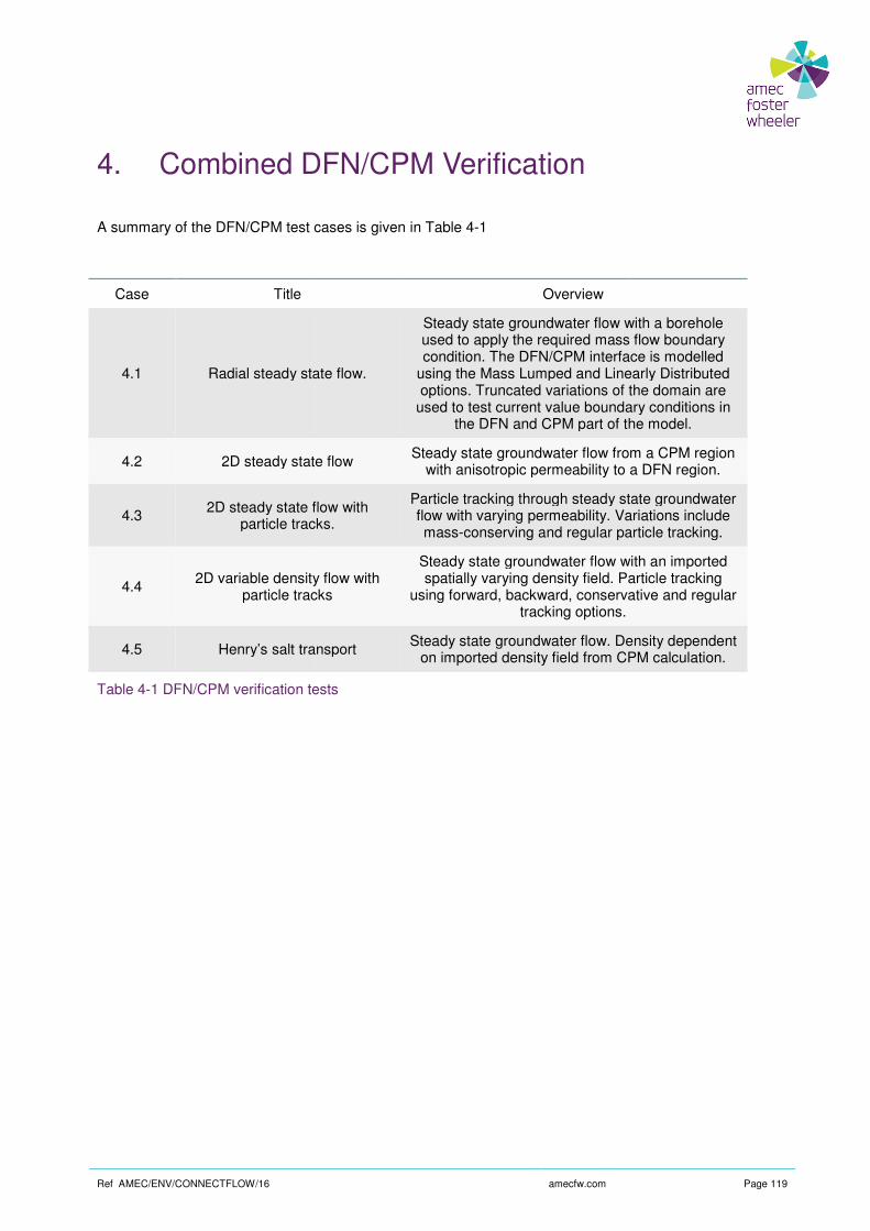
Ref AMEC/ENV/CONNECTFLOW/16
4. Combined DFN/CPM Verification
A summary of the DFN/CPM test cases is given in
Case Title
4.1 Radial steady state flow.
4.2 2D steady state flow
4.3 2D steady state flow with
particle tracks.
4.4 2D variable density flow with
particle tracks
4.5 Henry’s salt transport
Table 4-1 DFN/CPM verification tests
amecfw.com
Combined DFN/CPM Verification
A summary of the DFN/CPM test cases is given in Table 4-1
Overview
Radial steady state flow.
Steady state groundwater flow with a borehole used to apply the required mass flow boundary condition. The DFN/CPM interface is modelled
using the Mass Lumped and Linearly Distributed options. Truncated variations of the domain are
used to test current value boundary conditions in the DFN and CPM part of the model.
2D steady state flow Steady state groundwater flow from a CPM region
with anisotropic permeability to a DFN reg
2D steady state flow with particle tracks.
Particle tracking through steady state groundwater flow with varying permeability. Variations include mass-conserving and regular particle tracking.
2D variable density flow with particle tracks
Steady state groundwater flow with an imported spatially varying density field. Particle tracking
using forward, backward, conservative and regultracking options.
Henry’s salt transport Steady state groundwater flow. Density dependent
on imported density field from CPM calculation.
DFN/CPM verification tests
Page 119
with a borehole used to apply the required mass flow boundary condition. The DFN/CPM interface is modelled
using the Mass Lumped and Linearly Distributed options. Truncated variations of the domain are
used to test current value boundary conditions in DFN and CPM part of the model.
Steady state groundwater flow from a CPM region with anisotropic permeability to a DFN region.
Particle tracking through steady state groundwater flow with varying permeability. Variations include
conserving and regular particle tracking.
Steady state groundwater flow with an imported spatially varying density field. Particle tracking
using forward, backward, conservative and regular
Steady state groundwater flow. Density dependent on imported density field from CPM calculation.

Ref AMEC/ENV/CONNECTFLOW/16
4.1 Radial Steady State Flow
4.1.1 Overview
This case models steady groundwater flow in a 2D disk where water is removed from the centre at a constant rate and the outer disk bounda
4.1.2 Problem Definition
The problem definition and solution is taken from Feftra [The model domain is split up into two regions, fractured rock in the centre of the disk surrounded by porous medium rock, as is illustrated in rock are selected such that the solution is the same as in case
Figure 4-1 Schematic of problem definition
Symbol
h
Q
Kf Hydraulic Conductivity Fracture
Kr Hydraulic Conductivity Rock
R
e
d
r
ρ
µ
g
Table 4-2 Input parameters
amecfw.com
Radial Steady State Flow
This case models steady groundwater flow in a 2D disk where water is removed from the centre at a constant rate and the outer disk boundary is maintained at a constant head.
The problem definition and solution is taken from Feftra [3] and is the DFN/CPM equivalent of case The model domain is split up into two regions, fractured rock in the centre of the disk surrounded by porous medium rock, as is illustrated in Figure 4-1. The properties of the fractures and porous medium rock are selected such that the solution is the same as in case 2.1.
Schematic of problem definition
Parameter Value
Head at r = R 0 m
Outflow from disk 8.17E-6 m
Hydraulic Conductivity Fracture 8.17E-3
Hydraulic Conductivity Rock 8.17E-7 m/s
Radius of rock 2000 m
Aperture of fracture 1.0E-4 m
Thickness of disk 1 m
Radial distance from axis 0-2000 m
Density 1000 kg/m
Viscosity 1.0E-3 Pa.s
Gravity 9.8 m/s
Page 120
This case models steady groundwater flow in a 2D disk where water is removed from the centre at a
] and is the DFN/CPM equivalent of case 2.1. The model domain is split up into two regions, fractured rock in the centre of the disk surrounded by
. The properties of the fractures and porous medium
Value
0 m
6 m3/s
3 m/s
7 m/s
2000 m
4 m
1 m
2000 m
1000 kg/m3
Pa.s
9.8 m/s2

Ref AMEC/ENV/CONNECTFLOW/16
The product of the hydraulic conductivities and thickness are chosen to be constant across the domain, with the hydraulic conductivity of the fracture
µ
ρ
12
2ge
K f =
The outflow rate is then set to make the solution the same as in
4.1.3 Variations
The modelled domain consists of a 15 degree sector. The region r<1000 m is modelled as a planar tessellated fracture using the DFN model. The region 1000<r<2000 m is modelled as model. The fractures and mesh are shown in
Figure 4-2 Fractures and CPM Mesh
4.1.3.1 Mass lumped ConnectFlow Fluxes
The interface between the two regions is modelled using the interface options, FLUX and MASS LUMP NAPSAC FLUXES
4.1.3.2 Current Value in CPM Region
In this variant, the modelled domain is truncated at a radius of 1500the CPM case 2.1.3.1 is applied as a pressure boundary condition. The interface option is used.
amecfw.com
The product of the hydraulic conductivities and thickness are chosen to be constant across the domain, with the hydraulic conductivity of the fracture being derived from the fracture aperture as follows.
The outflow rate is then set to make the solution the same as in 2.1.5.
The modelled domain consists of a 15 degree sector. The region r<1000 m is modelled as a planar tessellated fracture using the DFN model. The region 1000<r<2000 m is modelled as model. The fractures and mesh are shown in Figure 4-2.
Fractures and CPM Mesh
lumped ConnectFlow Fluxes
The interface between the two regions is modelled using the interface options, CONSERVE FRACTURE MASS LUMP NAPSAC FLUXES.
Current Value in CPM Region
In this variant, the modelled domain is truncated at a radius of 1500 m, and the interpolated solution from is applied as a pressure boundary condition. The MASS LUMP NAPSAC FLUXES
Page 121
The product of the hydraulic conductivities and thickness are chosen to be constant across the domain, being derived from the fracture aperture as follows.
The modelled domain consists of a 15 degree sector. The region r<1000 m is modelled as a planar tessellated fracture using the DFN model. The region 1000<r<2000 m is modelled as rock using the CPM
CONSERVE FRACTURE
m, and the interpolated solution from MASS LUMP NAPSAC FLUXES

Ref AMEC/ENV/CONNECTFLOW/16
4.1.3.3 Current Value in DFN Region
In this variant, the modelled domain is truncated at a radius of 250 m, and the interpolated solution from the CPM case 2.1.3.1 is applied as a pressure boundary condition. The interface option is used.
4.1.3.4 Linearly Distributed ConnectFlow Fluxes
The interface between the two regions is modelled using the default interface options, FRACTURE FLUX and LINEARLY DISTRIBUTE NAPSAC FLUXES
4.1.4 Results
The analytical solution is given by
)ln(2
)()(r
R
Kd
QRhrh
π−=
The results from DFN/CPM calculation show good overall agreement with the analytical solution, as illustrated in Figure 4-3 to Figure 4linear distributed fluxes method gives a smoother and more accurate solution.
Figure 4-3 Variation of head with distance using a mass lumped DFN/CPM interface
-8
-7
-6
-5
-4
-3
-2
-1
0
0 500
Head
[m
]
amecfw.com
Current Value in DFN Region
In this variant, the modelled domain is truncated at a radius of 250 m, and the interpolated solution from is applied as a pressure boundary condition. The MASS LUMP NAPSAC FLUXES
Linearly Distributed ConnectFlow Fluxes
The interface between the two regions is modelled using the default interface options, LINEARLY DISTRIBUTE NAPSAC FLUXES.
The analytical solution is given by
The results from DFN/CPM calculation show good overall agreement with the analytical solution, as 4-6. The mass lumping method is more computationally efficient, but the
ted fluxes method gives a smoother and more accurate solution.
Variation of head with distance using a mass lumped DFN/CPM interface
1000 1500 2000
Radius [m]
ConnectFlow
Analytical Solution
Page 122
In this variant, the modelled domain is truncated at a radius of 250 m, and the interpolated solution from MASS LUMP NAPSAC FLUXES
The interface between the two regions is modelled using the default interface options, CONSERVE
The results from DFN/CPM calculation show good overall agreement with the analytical solution, as . The mass lumping method is more computationally efficient, but the
Variation of head with distance using a mass lumped DFN/CPM interface
ConnectFlow
Analytical Solution

Ref AMEC/ENV/CONNECTFLOW/16
Figure 4-4 Variation of head with distance using a current value boundary in the CPM region and a mass lumped DFN/CPM interface
Figure 4-5 Variation of head with distance using a current value boundary in the DFN reglumped DFN/CPM interface
-8
-7
-6
-5
-4
-3
-2
-1
0
0 500
Head
[m
]
-8
-7
-6
-5
-4
-3
-2
-1
0
0 500
Head
[m
]
amecfw.com
Variation of head with distance using a current value boundary in the CPM region and a mass lumped DFN/CPM interface
Variation of head with distance using a current value boundary in the DFN reglumped DFN/CPM interface
1000 1500 2000
Radius [m]
ConnectFlow
Analytical Solution
1000 1500 2000
Radius [m]
ConnectFlow
Analytical Solution
Page 123
Variation of head with distance using a current value boundary in the CPM region and a mass
Variation of head with distance using a current value boundary in the DFN region and a mass
ConnectFlow
Analytical Solution
ConnectFlow
Analytical Solution

Ref AMEC/ENV/CONNECTFLOW/16
Figure 4-6 Variation of head with distance using a linearly distributed DFN/CPM interface
4.2 Flow to Fracture Network
4.2.1 Overview
This case models steady state groundwaterflow enters the network through porous medium rock with anisotropic permeability.
4.2.2 Problem Definition
The problem is a variant of test 3.6
Figure 4-7 Schematic of problem definition
The fracture properties are the same as in Section
The CPM properties are defined in such a way as to ensure the following conditions at the interface.
-8
-7
-6
-5
-4
-3
-2
-1
0
0 500
Head
[m
]
amecfw.com
Variation of head with distance using a linearly distributed DFN/CPM interface
Flow to Fracture Network
This case models steady state groundwater flow in a simple two-dimensional fracture network where the flow enters the network through porous medium rock with anisotropic permeability.
3.6, as illustrated in Figure 4-7.
Schematic of problem definition
The fracture properties are the same as in Section 3.6.3.2.
The CPM properties are defined in such a way as to ensure the following conditions at the interface.
1000 1500 2000
Radius [m]
ConnectFlow
Analytical Solution
Page 124
Variation of head with distance using a linearly distributed DFN/CPM interface
dimensional fracture network where the flow enters the network through porous medium rock with anisotropic permeability.
The CPM properties are defined in such a way as to ensure the following conditions at the interface.
ConnectFlow
Analytical Solution

Ref AMEC/ENV/CONNECTFLOW/16
1== CPMDFN hh m
hKAQQ CPMDFN ∇==
Where K is the hydraulic conductivity
The first equation defines the head gradient in the CPM region, and the second is then used in conjunction with the DFN analytical value of Q to obtain K.
As the flow needs to enter the DFN region throucomponent to the flow in the CPM region. In order to avoid this impacting the head at the fracture inflows the vertical component or permeability is set to be 1000 times higher than the horizontal compo
4.2.3 Results
The calculated heads are all within 4% of the analytical solution.
Intersection ConnectFlow
a 0.062
b 0.936
c 0.598
Table 4-3 Heads at fracture intersections
4.3 2D Steady State Flow with Particle Tracks
4.3.1 Overview
This case is taken from Level 3 of the international HYDROCOIN project for verification of groundwater flow codes [31]. It models steady state flow in a tworegion of higher permeability.
The case has a non-uniform analytical solution and is used in the HYDROCOIN study to test particle tracking.
amecfw.com
Where K is the hydraulic conductivity and A the cross sectional area of the CPM region.
The first equation defines the head gradient in the CPM region, and the second is then used in conjunction with the DFN analytical value of Q to obtain K.
As the flow needs to enter the DFN region through the three fractures, there will also be a vertical component to the flow in the CPM region. In order to avoid this impacting the head at the fracture inflows the vertical component or permeability is set to be 1000 times higher than the horizontal compo
The calculated heads are all within 4% of the analytical solution.
ConnectFlow Analytical % Error
0.061 1.42%
0.968 3.36%
0.598 0.600 0.19%
Heads at fracture intersections
2D Steady State Flow with Particle Tracks
This case is taken from Level 3 of the international HYDROCOIN project for verification of groundwater ]. It models steady state flow in a two-dimensional vertical slice of rock, containing a circular
uniform analytical solution and is used in the HYDROCOIN study to test particle
Page 125
and A the cross sectional area of the CPM region.
The first equation defines the head gradient in the CPM region, and the second is then used in conjunction
gh the three fractures, there will also be a vertical component to the flow in the CPM region. In order to avoid this impacting the head at the fracture inflows the vertical component or permeability is set to be 1000 times higher than the horizontal component.
% Error
1.42%
3.36%
0.19%
This case is taken from Level 3 of the international HYDROCOIN project for verification of groundwater tical slice of rock, containing a circular
uniform analytical solution and is used in the HYDROCOIN study to test particle
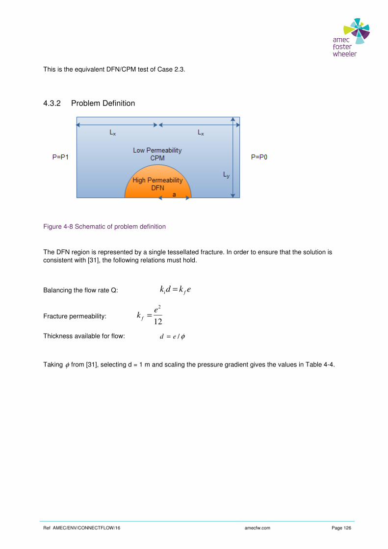
Ref AMEC/ENV/CONNECTFLOW/16
This is the equivalent DFN/CPM test of C
4.3.2 Problem Definition
Figure 4-8 Schematic of problem definition
The DFN region is represented by a single tessellated fracture. In orconsistent with [31], the following relations must hold.
Balancing the flow rate Q:
Fracture permeability: k
Thickness available for flow:
Taking φ from [31], selecting d = 1 m and scaling the pressure gradient gives the values in
amecfw.com
the equivalent DFN/CPM test of Case 2.3.
Schematic of problem definition
The DFN region is represented by a single tessellated fracture. In order to ensure that the solution is ], the following relations must hold.
ekdk fi =
12
2e
k f =
φ/ed =
], selecting d = 1 m and scaling the pressure gradient gives the values in
Page 126
der to ensure that the solution is
], selecting d = 1 m and scaling the pressure gradient gives the values in Table 4-4.

Ref AMEC/ENV/CONNECTFLOW/16
Symbol
Lx
Ly Vertical outer region distance
a
P1
P0
ko
ki
kf
e
d
φ
fφ
ρ
µ
Table 4-4 Input parameters
Eight particle tracks are released 50 m upstream of the disk centre and at Y values of 10, 12, 14, 16, 18, 20, 22 and 24 m.
The analytical solution for the pathlines is given in the HYDROC
)1/()(
)(2
2
oi
oi
kk
kk
r
aoyy
+
−+= for r > a
o
oi
k
kk
oyy2
)( += for r < a
Where r is the distance from the centre of the disk and ya long distance away from the origin.
amecfw.com
Parameter Value
Upstream and downstream distances
250 m
Vertical outer region distance 240 m
Radius of inner disk 10 m
Upstream pressure 3.0E-4 Pa
Downstream pressure -3.0E-4 Pa
Permeability of outer region 8.333E-
Permeability of inner region 8.333E-
Fracture permeability 8.333E-
Fracture thickness 0.1 m
CPM thickness 1 m
Porosity 0.1
Fracture Porosity 1.0
Density 1000 kg/m
Viscosity 1.0E-3 Pa.s
Eight particle tracks are released 50 m upstream of the disk centre and at Y values of 10, 12, 14, 16, 18,
The analytical solution for the pathlines is given in the HYDROCOIN report [7] as
Where r is the distance from the centre of the disk and y0 is a constant representing the height of the track a long distance away from the origin.
Page 127
Value
250 m
240 m
10 m
4 Pa
4 Pa
-7 m2
-5 m2
-4 m2
0.1 m
1 m
0.1
1.0
1000 kg/m3
3 Pa.s
Eight particle tracks are released 50 m upstream of the disk centre and at Y values of 10, 12, 14, 16, 18,
esenting the height of the track

Ref AMEC/ENV/CONNECTFLOW/16
4.3.3 Variations
4.3.3.1 Regular Particle Tracking
Regular particle tracking was used within the CPM region. The mesh around the DFN region is shown in Figure 4-9.
Figure 4-9 CPM wrapped mesh
The tessellated fractures within the inner region are shown in
Figure 4-10 Tessellated fractures (larger scale image).
4.3.3.2 Mass Conserving Particle Tracking
Mass conserving particle tracking was used withishown in Figure 4-11.
amecfw.com
Regular Particle Tracking
Regular particle tracking was used within the CPM region. The mesh around the DFN region is shown in
The tessellated fractures within the inner region are shown in Figure 4-10.
Tessellated fractures (larger scale image).
Mass Conserving Particle Tracking
Mass conserving particle tracking was used within the CPM region. The mesh around the DFN region is
Page 128
Regular particle tracking was used within the CPM region. The mesh around the DFN region is shown in
n the CPM region. The mesh around the DFN region is

Ref AMEC/ENV/CONNECTFLOW/16
Figure 4-11 CPM regular mesh
The tessellated fractures within the inner region are shown in
Figure 4-12 Tessellated fractures (larger scale im
4.3.4 Results
The particle tracks within the DFN part of the model are treated in a stochastic manner, allowing different tracks to take different paths. Ten particles were released from each of the starting positions and the results for regular particle tracking are shown in
For the tracks that do not pass through the DFN region, the results are within 1% ofor the regular particle tracking, and within 2% of the analytical solution for the mass conserving particle tracking.
The stochastic tracks have more variation as expected, however the average tracks starting from each position also have a travel time and final location within 1% of the analytical solution for the regular particle tracks and within 2% of the analytical solution for the mass conserving particle tracking.
amecfw.com
ated fractures within the inner region are shown in Figure 4-12.
Tessellated fractures (larger scale image).
The particle tracks within the DFN part of the model are treated in a stochastic manner, allowing different tracks to take different paths. Ten particles were released from each of the starting positions and the
tracking are shown in Figure 4-13 and Figure 4-14.
For the tracks that do not pass through the DFN region, the results are within 1% ofor the regular particle tracking, and within 2% of the analytical solution for the mass conserving particle
The stochastic tracks have more variation as expected, however the average tracks starting from each also have a travel time and final location within 1% of the analytical solution for the regular particle
tracks and within 2% of the analytical solution for the mass conserving particle tracking.
Page 129
The particle tracks within the DFN part of the model are treated in a stochastic manner, allowing different tracks to take different paths. Ten particles were released from each of the starting positions and the
For the tracks that do not pass through the DFN region, the results are within 1% of the analytical solution for the regular particle tracking, and within 2% of the analytical solution for the mass conserving particle
The stochastic tracks have more variation as expected, however the average tracks starting from each also have a travel time and final location within 1% of the analytical solution for the regular particle
tracks and within 2% of the analytical solution for the mass conserving particle tracking.

Ref AMEC/ENV/CONNECTFLOW/16
Figure 4-13 Regular particle tracks
Figure 4-14 Stochastic behaviour of particle tracks
amecfw.com
Regular particle tracks
Stochastic behaviour of particle tracks
Page 130
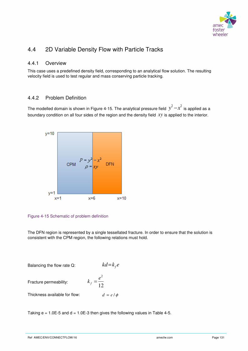
Ref AMEC/ENV/CONNECTFLOW/16
4.4 2D Variable Density Flow with Particle Tracks
4.4.1 Overview
This case uses a predefined density field, corresponding to an analvelocity field is used to test regular and mass conserving particle tracking.
4.4.2 Problem Definition
The modelled domain is shown in
boundary condition on all four sides of the region and the density field
Figure 4-15 Schematic of problem definition
The DFN region is represented by a single tessellated fracture. In order to ensure that the solution is consistent with the CPM region, the following relations must hold.
Balancing the flow rate Q:
Fracture permeability: k
Thickness available for flow:
Taking e = 1.0E-5 and d = 1.0E-3 then gives the following values in
amecfw.com
2D Variable Density Flow with Particle Tracks
This case uses a predefined density field, corresponding to an analytical flow solution. The resulting velocity field is used to test regular and mass conserving particle tracking.
The modelled domain is shown in Figure 4-15. The analytical pressure field 2
xy −boundary condition on all four sides of the region and the density field xy is applied to the interior.
Schematic of problem definition
The DFN region is represented by a single tessellated fracture. In order to ensure that the solution is consistent with the CPM region, the following relations must hold.
ekkd f=
12
2e
k f =
φ/ed =
3 then gives the following values in Table 4-5.
Page 131
ytical flow solution. The resulting
2x is applied as a
is applied to the interior.
The DFN region is represented by a single tessellated fracture. In order to ensure that the solution is

Ref AMEC/ENV/CONNECTFLOW/16
Symbol
k
kf
e
d
φ
µ
Table 4-5 Input parameters
4.4.3 Variations
4.4.3.1 Forward Particle Tracking
This variant tracks 10 particles starting from the upper left hand corner of the The tracks subsequently pass through the DFN region where they behave in a stochastic manner, allowing different tracks to take different paths.
4.4.3.2 Backward Particle Tracking
This variant performs backward tracking on 10 particlwhich corresponds to the same analytical path as the forward track in variation
4.4.3.3 Mass Conserving Particl
This variant tracks ten particles starting from x=1.5, y = 9.5 and uses the mass conserving particle tracking option. The tracks subsequently pass through the DFN region where they behave in a stochastic manner, allowing different tracks to take different paths.
4.4.4 Results
4.4.4.1 Analytical solution
Substituting the Darcy flow equation into the continuity equation gives
0))(.( =∇∇ Pk
µρϕ
amecfw.com
Parameter Value
Permeability of CPM region 8.333E-
Fracture permeability 8.333E-
Fracture thickness 1.0E-5 m
CPM thickness 1.0E-3 m
Porosity 0.01
Viscosity 1.0E-3 Pa.s
Forward Particle Tracking
This variant tracks 10 particles starting from the upper left hand corner of the CPM region at x=1.5, y = 9.5. The tracks subsequently pass through the DFN region where they behave in a stochastic manner, allowing different tracks to take different paths.
Backward Particle Tracking
This variant performs backward tracking on 10 particles ending at x=9.07, y=1.57 within the DFN region, which corresponds to the same analytical path as the forward track in variation 4.4.3.1
Mass Conserving Particle Tracking
This variant tracks ten particles starting from x=1.5, y = 9.5 and uses the mass conserving particle tracking option. The tracks subsequently pass through the DFN region where they behave in a stochastic manner,
different paths.
Substituting the Darcy flow equation into the continuity equation gives
Page 132
Value
-14 m2
-12 m2
5 m
3 m
0.01
3 Pa.s
CPM region at x=1.5, y = 9.5. The tracks subsequently pass through the DFN region where they behave in a stochastic manner, allowing
es ending at x=9.07, y=1.57 within the DFN region, 4.4.3.1.
This variant tracks ten particles starting from x=1.5, y = 9.5 and uses the mass conserving particle tracking option. The tracks subsequently pass through the DFN region where they behave in a stochastic manner,

Ref AMEC/ENV/CONNECTFLOW/16
Gravity is omitted as 0=∂
∂
z
ρ.
Substituting in the proposed solution
0))((.( 22 =−∇∇ xyxy
which reduces to
4)2()2( 22 −=∂
∂+−
∂
∂xyxy
yyx
x
This confirms that xy=ρ and P
From the pressure field, the particle tracks can then be determined as
represents the starting location of the particle track. The corresponding travel time being
4.4.4.2 Pressure and Density Fields
Figure 4-16 and Figure 4-17 show the pressure and density fields. The former being calculated and the latter being prescribed.
amecfw.com
Substituting in the proposed solution xy=ρ and 22
xyP −= then gives
04 =+ xyxy
22xyP −= is a solution of the Darcy flow equations with variable density.
From the pressure field, the particle tracks can then be determined as x
yxy 00= where
represents the starting location of the particle track. The corresponding travel time being
sity Fields
show the pressure and density fields. The former being calculated and the
Page 133
is a solution of the Darcy flow equations with variable density.
where 00, yx
represents the starting location of the particle track. The corresponding travel time being )ln(2 ox
x
kt
µφ= .
show the pressure and density fields. The former being calculated and the

Ref AMEC/ENV/CONNECTFLOW/16
Figure 4-16 Calculated residual pressure
amecfw.com
Calculated residual pressures.
Page 134

Ref AMEC/ENV/CONNECTFLOW/16
Figure 4-17 Applied densities.
4.4.4.3 Forward particle tracking
Figure 4-18 shows 10 particle tracks released from the DFN region the tracks behave in a stochastic manner. The background of the plot is coloured by residual pressure.
amecfw.com
Forward particle tracking
shows 10 particle tracks released from the top left corner of the CPM region. On entering the DFN region the tracks behave in a stochastic manner. The background of the plot is coloured by residual
Page 135
top left corner of the CPM region. On entering the DFN region the tracks behave in a stochastic manner. The background of the plot is coloured by residual

Ref AMEC/ENV/CONNECTFLOW/16
Figure 4-18 Forward particle tracks
An averaged particle track plot is compared against the analytical solution in agreeing to within 2% of the analytical solution for position and in the DFN region, it is necessary to set the model reference density to a value representative of that of the fluid which the track passes through.
Figure 4-19 Averaged forward tracks
0
1
2
3
4
5
6
7
8
9
10
0 2 4
X [m]
Y [
m]
amecfw.com
Forward particle tracks
veraged particle track plot is compared against the analytical solution in Figure agreeing to within 2% of the analytical solution for position and travel time. In order to predict travel times in the DFN region, it is necessary to set the model reference density to a value representative of that of the fluid which the track passes through.
Averaged forward tracks
6 8 10
X [m]
ConnectFlow
Analytical Solution
Page 136
Figure 4-19, the results travel time. In order to predict travel times
in the DFN region, it is necessary to set the model reference density to a value representative of that of the
Analytical Solution

Ref AMEC/ENV/CONNECTFLOW/16
4.4.4.4 Backward Particle Tracking
Figure 4-20 shows 10 particle tracks tracked backwards from the lower right hand corner of the DFN region. Within the DFN region the tracks behave in a stochastic manner. The background of the plot is coloured by residual pressure.
Figure 4-20 Backward particle tracks
An averaged particle track plot is compared against the analytical solution in agreeing to within 2% of the analytical solution for position
amecfw.com
Backward Particle Tracking
shows 10 particle tracks tracked backwards from the lower right hand corner of the DFN in the DFN region the tracks behave in a stochastic manner. The background of the plot is
Backward particle tracks
An averaged particle track plot is compared against the analytical solution in Figure agreeing to within 2% of the analytical solution for position and travel time.
Page 137
shows 10 particle tracks tracked backwards from the lower right hand corner of the DFN in the DFN region the tracks behave in a stochastic manner. The background of the plot is
Figure 4-21, the results

Ref AMEC/ENV/CONNECTFLOW/16
Figure 4-21 Averaged backward particle tracks
4.4.4.5 Mass Conserving Particle Tracking
The mass conserving tracks behave in a similar manner to the nonresults agreeing to within 2% of the analytical solution for position and travel time
Figure 4-22 Averaged mass conserving particle tracks
0
1
2
3
4
5
6
7
8
9
0 2 4
X [m]
Y [
m]
0
1
2
3
4
5
6
7
8
9
10
0 2 4
X [m]
Y [
m]
amecfw.com
Averaged backward particle tracks
Mass Conserving Particle Tracking
The mass conserving tracks behave in a similar manner to the non-mass conserving equivalents, with the ts agreeing to within 2% of the analytical solution for position and travel time
mass conserving particle tracks
6 8 10
X [m]
ConnectFlow
Analytical Solution
6 8 10
X [m]
ConnectFlow
Analytical Solution
Page 138
mass conserving equivalents, with the
Analytical Solution
Analytical Solution

Ref AMEC/ENV/CONNECTFLOW/16
4.5 Henry’s Salt Transport Using Interpolated Density
4.5.1 Overview
This case considers the groundwater pressures arising from a spatially varying density field.
The geometry, boundary conditions and density field are taken from the modified Henry CPM
4.5.2 Problem Definition
A schematic of the test case is shown in
Figure 4-23 Henry’s Problem
Symbol
K Hydraulic conductivity of rock
Q
ρ
φ
e
Table 4-6 Input parameters
The DFN domain is represented by a single fracturefracture thickness is set to 1.8516Em/s. The DFN region covers the left 75% of the domain, which has been selected so that the interfbetween the CPM and DFN region is in a location where the density and pressure fields are rapidly changing.
amecfw.com
Henry’s Salt Transport Using Interpolated Density
considers the groundwater pressures arising from a spatially varying density field.
The geometry, boundary conditions and density field are taken from the modified Henry CPM
A schematic of the test case is shown in Figure 4-23 and the input parameters are given in
Parameter Value
Hydraulic conductivity of rock 1.0E-2 m/s
Freshwater inflow per unit depth
9.43E-5 m
Density Interpolated
Porosity 0.35
Fracture thickness 1.8516E-
The DFN domain is represented by a single fracture tessellated into 0.025 m square subfracture thickness is set to 1.8516E-4 m in order to generate the desired hydraulic conductivity of 1.0Em/s. The DFN region covers the left 75% of the domain, which has been selected so that the interfbetween the CPM and DFN region is in a location where the density and pressure fields are rapidly
Page 139
considers the groundwater pressures arising from a spatially varying density field.
The geometry, boundary conditions and density field are taken from the modified Henry CPM Case 2.8.
and the input parameters are given in Table 4-6.
Value
2 m/s
5 m2/s
Interpolated
0.35
-4 m
tessellated into 0.025 m square sub-fractures. The 4 m in order to generate the desired hydraulic conductivity of 1.0E-2
m/s. The DFN region covers the left 75% of the domain, which has been selected so that the interface between the CPM and DFN region is in a location where the density and pressure fields are rapidly

Ref AMEC/ENV/CONNECTFLOW/16
The CPM region has thickness /e
The CPM region is meshed with the same spatial resolution as the sub
The interpolated density field used is shown in
Figure 4-24 Interpolated density field
4.5.3 Results
The residual pressure field of the DFN/CPM calculation is compared against the CPM pressure field from case 2.8, the latter having been separately checked against the analytical solution via the salt concentration solution.
Plots of the two pressure fields are shown in vary in shape near the inflow, in absolute terms the pressure fields agree to within 5%.
The influence of the density variation in this test case was checked by redensity instead of the interpolated density. In this case the difference in compared with the CPM solution.
amecfw.com
φ/ so that the cross sectional area available to flow remains constant.
The CPM region is meshed with the same spatial resolution as the sub-fractures.
The interpolated density field used is shown in Figure 4-24.
Interpolated density field
The residual pressure field of the DFN/CPM calculation is compared against the CPM pressure field from , the latter having been separately checked against the analytical solution via the salt
Plots of the two pressure fields are shown in Figure 4-25 and Figure 4-26. Although the pressure contours r the inflow, in absolute terms the pressure fields agree to within 5%.
The influence of the density variation in this test case was checked by re-running with a constant average density instead of the interpolated density. In this case the difference in the pressure fields was 30% when
Page 140
so that the cross sectional area available to flow remains constant.
The residual pressure field of the DFN/CPM calculation is compared against the CPM pressure field from , the latter having been separately checked against the analytical solution via the salt
. Although the pressure contours r the inflow, in absolute terms the pressure fields agree to within 5%.
running with a constant average the pressure fields was 30% when

Ref AMEC/ENV/CONNECTFLOW/16
Figure 4-25 Residual pressure in the DFN/CPM model
Figure 4-26 Residual pressure in the CPM model
amecfw.com
Residual pressure in the DFN/CPM model
Residual pressure in the CPM model
Page 141

Ref AMEC/ENV/CONNECTFLOW/16
5. Further Testing
This section references further testing that has taken place on the ConnectFlow suite of software, which complements and extends the testing covered in the earlier sections.
5.1 Continuum Porous Media
5.1.1 Verification
5.1.1.1 SKB – Implicit Representation of Fractures
Section 3.3 of SKB report R-01-49 [rock matrix by modifying CPM permeabilties. The approach is tested on a simple 3D case with a semianalytical solution. The results are all within 20% of the expected solution, with the accuracy improving for larger features. The algorithm allows small features to be modelled more accurately but with increased computational cost.
5.1.1.2 SKB – Heat Transport
Appendix F of SKB report R-06-98 [The first case models 1D heat conduction with a timecase models 1D heat conduction with a specifieHYDROCOIN Level 1 Test Case 5 for transient thermal convection in a saturated permeable medium containing a heat source with decaying power output. The first two cases have an analytical solution anthe third a semi-analytical solution. In all cases ConnectFlow shows excellent agreement with the expected solutions.
5.1.1.3 SKB R-09-24
Appendix G of SKB report R-09-24 [modelling the inflow of fresh water into a repository under open repository conditions. The ConnectFlow simulation modeled the repository region as a combined DFN/CPM, with boundary conditions being applied from a separate DFN site scale model. fine grid refinement around the tunnelsthe repository agreed to within 20%.
amecfw.com
Further Testing
This section references further testing that has taken place on the ConnectFlow suite of software, which complements and extends the testing covered in the earlier sections.
Continuum Porous Media
Implicit Representation of Fractures
49 [32] describes the modelling of a set of fractures within a background rock matrix by modifying CPM permeabilties. The approach is tested on a simple 3D case with a semianalytical solution. The results are all within 20% of the expected solution, with the accuracy improving for larger features. The algorithm allows small features to be modelled more accurately but with increased
98 [33] describes three verification tests on heat transport in ConnectFlow. D heat conduction with a time-varying temperature boundary condition. The second
case models 1D heat conduction with a specified heat flux boundary condition. The final case models the HYDROCOIN Level 1 Test Case 5 for transient thermal convection in a saturated permeable medium containing a heat source with decaying power output. The first two cases have an analytical solution an
analytical solution. In all cases ConnectFlow shows excellent agreement with the expected
24 [34] describes a comparison of DarcyTools and ConnectFlow in water into a repository under open repository conditions. The ConnectFlow
simulation modeled the repository region as a combined DFN/CPM, with boundary conditions being applied from a separate DFN site scale model. DarcyTools used a single regional-scale Efine grid refinement around the tunnels. Both models used the same Hydro-DFN data. The overall inflow to the repository agreed to within 20%.
Page 142
This section references further testing that has taken place on the ConnectFlow suite of software, which
] describes the modelling of a set of fractures within a background rock matrix by modifying CPM permeabilties. The approach is tested on a simple 3D case with a semi-analytical solution. The results are all within 20% of the expected solution, with the accuracy improving for larger features. The algorithm allows small features to be modelled more accurately but with increased
] describes three verification tests on heat transport in ConnectFlow. varying temperature boundary condition. The second
d heat flux boundary condition. The final case models the HYDROCOIN Level 1 Test Case 5 for transient thermal convection in a saturated permeable medium containing a heat source with decaying power output. The first two cases have an analytical solution and
analytical solution. In all cases ConnectFlow shows excellent agreement with the expected
] describes a comparison of DarcyTools and ConnectFlow in water into a repository under open repository conditions. The ConnectFlow
simulation modeled the repository region as a combined DFN/CPM, with boundary conditions being scale ECPM model with
DFN data. The overall inflow to

Ref AMEC/ENV/CONNECTFLOW/16
5.1.1.4 ANDRA
A verification exercise for ConnectFlow has been performed for ANDRA [groundwater flow and radionuclide transport problems were investigated. The exercise included cases that were diffusion dominated, cases that were advection and dispersion dominated, cases in twodimensions, and cases with permeability contrasts between regions of the models such that the dominant flow and transport processes differed between the regions. With appropriate choices of the grid, the initial and boundary conditions, and the timethe analytical solutions given for all cases considered.
5.1.1.5 KBS-3
ConnectFlow has also been used in two reviews of repository assessments. These reviews compared the results obtained using different programs for the sameKBS-3 study [36], the groundwater heads obtained using ConnectFlow were compared with those obtained using the program GWHRT, for several different cases. In every case, the results agreed to at least six significant figures (the number of figures listed for the output from GWHRT). This gives great confidence that both programs were coded correctly.
5.1.1.6 Gewähr
Results obtained using ConnectFlow were also compared with results obtained using the FEM301 program for the Swiss Project Gewähr [slightly from those obtained using FEM301. These differences were traced to discrepancies between the FEM301 program and its documentation, and differences between treatment of highly distorted elements. When an appropriate temporary modification was made to ConnectFlow to enable it to mimic the behaviour of FEM301, the results obtained agreed to within five significant figures with those obtained from FEM301. It should be stressed that the initial differences were not due to any problems with ConnectFlow.
5.1.1.7 Nirex
The results of a Monte-Carlo study of dispersion in a heterogeneous porous medium [and quite stringent test of the groundwater flow and particle transport algorithms used in ConnectFlow. The fact that good agreement could be obtained between the analytical and numerical results for the dispersion of the particles indicates that ConnectFlow provided an accuratflow in a heterogeneous permeability field. This case therefore also builds confidence in the correctness of ConnectFlow.
amecfw.com
A verification exercise for ConnectFlow has been performed for ANDRA [35]. Cases covering a range of groundwater flow and radionuclide transport problems were investigated. The exercise included cases that were diffusion dominated, cases that were advection and dispersion dominated, cases in two
s with permeability contrasts between regions of the models such that the dominant flow and transport processes differed between the regions. With appropriate choices of the grid, the initial and boundary conditions, and the time-stepping scheme, ConnectFlow was found to accurately reproduce the analytical solutions given for all cases considered.
ConnectFlow has also been used in two reviews of repository assessments. These reviews compared the results obtained using different programs for the same finite-element model. In a review of the Swedish
], the groundwater heads obtained using ConnectFlow were compared with those obtained using the program GWHRT, for several different cases. In every case, the results agreed to at
gnificant figures (the number of figures listed for the output from GWHRT). This gives great confidence that both programs were coded correctly.
Results obtained using ConnectFlow were also compared with results obtained using the FEM301 or the Swiss Project Gewähr [37]. Initially, the results obtained using ConnectFlow differed
slightly from those obtained using FEM301. These differences were traced to discrepancies between the FEM301 program and its documentation, and differences between ConnectFlow and FEM301 in the treatment of highly distorted elements. When an appropriate temporary modification was made to ConnectFlow to enable it to mimic the behaviour of FEM301, the results obtained agreed to within five
e obtained from FEM301. It should be stressed that the initial differences were not due to any problems with ConnectFlow.
Carlo study of dispersion in a heterogeneous porous medium [st of the groundwater flow and particle transport algorithms used in ConnectFlow.
The fact that good agreement could be obtained between the analytical and numerical results for the dispersion of the particles indicates that ConnectFlow provided an accurate solution for the groundwater flow in a heterogeneous permeability field. This case therefore also builds confidence in the correctness of
Page 143
]. Cases covering a range of groundwater flow and radionuclide transport problems were investigated. The exercise included cases that were diffusion dominated, cases that were advection and dispersion dominated, cases in two- and three-
s with permeability contrasts between regions of the models such that the dominant flow and transport processes differed between the regions. With appropriate choices of the grid, the initial
ow was found to accurately reproduce
ConnectFlow has also been used in two reviews of repository assessments. These reviews compared the element model. In a review of the Swedish
], the groundwater heads obtained using ConnectFlow were compared with those obtained using the program GWHRT, for several different cases. In every case, the results agreed to at
gnificant figures (the number of figures listed for the output from GWHRT). This gives great
Results obtained using ConnectFlow were also compared with results obtained using the FEM301 ]. Initially, the results obtained using ConnectFlow differed
slightly from those obtained using FEM301. These differences were traced to discrepancies between the ConnectFlow and FEM301 in the
treatment of highly distorted elements. When an appropriate temporary modification was made to ConnectFlow to enable it to mimic the behaviour of FEM301, the results obtained agreed to within five
e obtained from FEM301. It should be stressed that the initial differences were
Carlo study of dispersion in a heterogeneous porous medium [38] provides a useful st of the groundwater flow and particle transport algorithms used in ConnectFlow.
The fact that good agreement could be obtained between the analytical and numerical results for the e solution for the groundwater
flow in a heterogeneous permeability field. This case therefore also builds confidence in the correctness of

Ref AMEC/ENV/CONNECTFLOW/16
5.1.1.8 Olkiluoto Site
A site scale comparison of FEFTRA and ConnectFlow was carried out as part of the FEFTR[3]. The study showed good agreement with regard to borehole pressures and flow rates near the repository. Flow path positions near the repository wwere shorter in FEFTRA as compared with ConnectFlow.
A further study [39] has compared modelling of pressures and salinity distributions in 15 deep core drilled boreholes between the codes and measuremengroundwater flow and solute transport over the last 8000 years.
5.2 Discrete Fracture Network
5.2.1 Verification
5.2.1.1 Stripa
This testing exercise formed part of an OECD/NEA [radioactive waste in crystalline rock, that involved a detailed characterisation of the abandoned iron ore mine at Stripa in central Sweden.
The testing compared fracture generatiocodes ConnectFlow, FracMan/MAFIC and FMG.
Eight test cases were considered and tsolutions and the results of FracMan/MAFIC and
5.2.1.2 Nirex
This study [41] compared transient flow for the fracture flow codes ConnectFlow and FracMan/MAFIC for six test cases. ConnectFlow and FracMan/MAFIC gave qualitatively similar results. However,quantitative differences were observed even for quite simple test networks. These are thought to be due to inadequate mesh discretisation of the source zone in FracMan/MAFIC. The ConnectFlow results for the early time behaviour compared well wsource zone responses that were inaccurate. The asymptotic ConnectFlow results were shown to tend to the steady state solutions.
5.3 Automated Testing
The test cases presented in this documentanalytical and benchmark data.
amecfw.com
A site scale comparison of FEFTRA and ConnectFlow was carried out as part of the FEFTR]. The study showed good agreement with regard to borehole pressures and flow rates near the
repository. Flow path positions near the repository were also in good agreement although the travel times were shorter in FEFTRA as compared with ConnectFlow.
] has compared modelling of pressures and salinity distributions in 15 deep core drilled boreholes between the codes and measurements based on simulations of the evolution of coupled groundwater flow and solute transport over the last 8000 years.
Discrete Fracture Network
This testing exercise formed part of an OECD/NEA [40] project relating to the final disposal of highly radioactive waste in crystalline rock, that involved a detailed characterisation of the abandoned iron ore mine at Stripa in central Sweden.
The testing compared fracture generation, steady state flow and particle tracking for the fracture flow , FracMan/MAFIC and FMG.
Eight test cases were considered and the ConnectFlow results compared well with available analytical solutions and the results of FracMan/MAFIC and FMG (when a formulation of the test case was possible).
] compared transient flow for the fracture flow codes ConnectFlow and FracMan/MAFIC for six test cases. ConnectFlow and FracMan/MAFIC gave qualitatively similar results. However,quantitative differences were observed even for quite simple test networks. These are thought to be due to inadequate mesh discretisation of the source zone in FracMan/MAFIC. The ConnectFlow results for the early time behaviour compared well with the available analytical solutions, whereas FracMan/MAFIC gave source zone responses that were inaccurate. The asymptotic ConnectFlow results were shown to tend to
Automated Testing
The test cases presented in this document can be automatically re-run to check the results against the
Page 144
A site scale comparison of FEFTRA and ConnectFlow was carried out as part of the FEFTRA verification ]. The study showed good agreement with regard to borehole pressures and flow rates near the
ere also in good agreement although the travel times
] has compared modelling of pressures and salinity distributions in 15 deep core drilled ts based on simulations of the evolution of coupled
] project relating to the final disposal of highly radioactive waste in crystalline rock, that involved a detailed characterisation of the granite formation in an
n, steady state flow and particle tracking for the fracture flow
he ConnectFlow results compared well with available analytical FMG (when a formulation of the test case was possible).
] compared transient flow for the fracture flow codes ConnectFlow and FracMan/MAFIC for six test cases. ConnectFlow and FracMan/MAFIC gave qualitatively similar results. However, significant quantitative differences were observed even for quite simple test networks. These are thought to be due to inadequate mesh discretisation of the source zone in FracMan/MAFIC. The ConnectFlow results for the
ith the available analytical solutions, whereas FracMan/MAFIC gave source zone responses that were inaccurate. The asymptotic ConnectFlow results were shown to tend to
run to check the results against the

Ref AMEC/ENV/CONNECTFLOW/16
This complements the regular ConnectFlow regression test suite, which consists of more than 200 tests and is used to comprehensively check results from new releaversions.
5.4 Peer Review
ConnectFlow is used by a wide variety There are representatives of both the regulatory bodies and the nuclear utilities. Many of thein the iConnect club and provide valuable feedback that helps enhance the software quality.
amecfw.com
This complements the regular ConnectFlow regression test suite, which consists of more than 200 tests and is used to comprehensively check results from new releases of the software against previous
ConnectFlow is used by a wide variety of organisations with an interest in radioactive waste disposal. There are representatives of both the regulatory bodies and the nuclear utilities. Many of thein the iConnect club and provide valuable feedback that helps enhance the software quality.
Page 145
This complements the regular ConnectFlow regression test suite, which consists of more than 200 tests ses of the software against previous
of organisations with an interest in radioactive waste disposal. There are representatives of both the regulatory bodies and the nuclear utilities. Many of these participate in the iConnect club and provide valuable feedback that helps enhance the software quality.

Ref AMEC/ENV/CONNECTFLOW/16
6. References
1 NAMMU Technical Summary, SA/ENV/CONNECTFLOW/8 May 2010
2 NAPSAC Technical Summary, SA/ENV/CONNECTFLOW/12 , May 2010
3 FEFTRA Verification, VTT Research Notes 2385, Espoo 2007.
4 de Marsily, G., 1986. Quantitative Hydrogeology Press INC, Orlando.
5 NEA/SKI, The International HYDROCOIN Project, Level 1: code verification,OECD Publications, 1988.
6 R. Atkinson, T.P. Cherill, A.W. Herbert, D.P. Hodgkinson, C.P. Jackson, J. Rae
and P.C. Robinson, Review of the grUKAEA Report AERE-R. 11140, 1984
7 NEA/SKI, The International HYDROCOIN Project, Level 3: uncertainty and sensitivity analysis ,OECD Publications, 1991.
8 A. Schäfers. Task Force on Engineered
Description. 2014.
9 Richards, L.A., 1931. Capillary conduction of liquids through porous mediums.Physics, 1(5), pp.318-333.
10 Zarba, R.L., Bouloutas, E.T. and Celia, M., 1990. unsaturated flow equation. Water Resources Research WRERAQ
11 Van Genuchten, M.T., 1980. A closedunsaturated soils. Soil science society of America journal
12 K. Pruess, TOUGH2 – A General Purpose Numerical Simulator for Multiphase Fluid and Heat Flow, Lawrence Berkeley Laboratory Report LBL
13 Bear Jacob, Hydraulics of Groundwater,1979, McGraw
14 Improving the worthiness of the Henry problem as a benchmark for density dependent ground water flows. Water Resources Research Vol 40, 2004.
15 A R Hoch, C P Jackson Rock-matrix diffusion in transport of salinity. SKB Report R
16 C. M. Oldenburg and K. Pruess. EOS7R: Radionuclide Transport for Tough2, Lawrence Berkley Laboratory Report LBL-34868, Berkley, CA, November 1995.
17 Javandel, I., C. Doughty, and C.American Geophys. Union, pp. 14
18 Joyce S, Applegate D, Appleyard P, Gordon A, Heath T, Hunter F, Hoek J, Jackson P, Swan D, Woollard H, 2014. Groundwater flow Svensk Kärnbränslehantering AB.
19 Parkhurst D L, Kipp K L, Charlton S R, 2010. PHAST Version 2: a program for simulatingflow, solute transport, and multicomponent geochemical reactiGeological Survey, Denver, Colorado.
amecfw.com
NAMMU Technical Summary, SA/ENV/CONNECTFLOW/8 May 2010
NAPSAC Technical Summary, SA/ENV/CONNECTFLOW/12 , May 2010
FEFTRA Verification, VTT Research Notes 2385, Espoo 2007.
de Marsily, G., 1986. Quantitative Hydrogeology – Groundwater Hydrology for Engineers. Academic
NEA/SKI, The International HYDROCOIN Project, Level 1: code verification,OECD Publications, 1988.
R. Atkinson, T.P. Cherill, A.W. Herbert, D.P. Hodgkinson, C.P. Jackson, J. Rae
and P.C. Robinson, Review of the groundwater flow and radionuclide transport modelling in KBSR. 11140, 1984
NEA/SKI, The International HYDROCOIN Project, Level 3: uncertainty and sensitivity analysis ,OECD
Task Force on Engineered Barrier Systems, “Code Validation”. Code Validation Task
Richards, L.A., 1931. Capillary conduction of liquids through porous mediums. Journal of Applied
Zarba, R.L., Bouloutas, E.T. and Celia, M., 1990. General mass-conservative numerical solution for the Water Resources Research WRERAQ, 26(7), pp.1483-
Van Genuchten, M.T., 1980. A closed-form equation for predicting the hydraulic conductivity of cience society of America journal, 44(5), pp.892-898.
A General Purpose Numerical Simulator for Multiphase Fluid and Heat Flow, Lawrence Berkeley Laboratory Report LBL–29400, 1991.
Bear Jacob, Hydraulics of Groundwater,1979, McGraw-Hill Inc.
Improving the worthiness of the Henry problem as a benchmark for density dependent ground water flows. Water Resources Research Vol 40, 2004.
matrix diffusion in transport of salinity. SKB Report R
C. M. Oldenburg and K. Pruess. EOS7R: Radionuclide Transport for Tough2, Lawrence Berkley 34868, Berkley, CA, November 1995.
C. Doughty, and C.-F. Tsang, Groundwater Transport, Handbook of Mathematical Models, American Geophys. Union, pp. 14-19, 1984.
Joyce S, Applegate D, Appleyard P, Gordon A, Heath T, Hunter F, Hoek J, Jackson P, Swan D, Woollard H, 2014. Groundwater flow and reactive transport modelling in ConnectFlow. SKB RSvensk Kärnbränslehantering AB.
Parkhurst D L, Kipp K L, Charlton S R, 2010. PHAST Version 2: a program for simulatingflow, solute transport, and multicomponent geochemical reactions. Techniques and Methods 6Geological Survey, Denver, Colorado.
Page 146
Engineers. Academic
NEA/SKI, The International HYDROCOIN Project, Level 1: code verification,OECD Publications, 1988.
oundwater flow and radionuclide transport modelling in KBS-3,
NEA/SKI, The International HYDROCOIN Project, Level 3: uncertainty and sensitivity analysis ,OECD
. Code Validation Task
Journal of Applied
conservative numerical solution for the -1496.
form equation for predicting the hydraulic conductivity of
A General Purpose Numerical Simulator for Multiphase Fluid and Heat Flow,
Improving the worthiness of the Henry problem as a benchmark for density dependent ground water
matrix diffusion in transport of salinity. SKB Report R-04-78.
C. M. Oldenburg and K. Pruess. EOS7R: Radionuclide Transport for Tough2, Lawrence Berkley
F. Tsang, Groundwater Transport, Handbook of Mathematical Models,
Joyce S, Applegate D, Appleyard P, Gordon A, Heath T, Hunter F, Hoek J, Jackson P, Swan D, and reactive transport modelling in ConnectFlow. SKB R-14-19,
Parkhurst D L, Kipp K L, Charlton S R, 2010. PHAST Version 2: a program for simulating groundwater ons. Techniques and Methods 6-A35, U.S.

Ref AMEC/ENV/CONNECTFLOW/16
20 Hall, P. (1982). "On Some Simple Estimates of an Exponent of Regular Variation". Statistical Society, Series B (Methodological) 44 (1): 37
21 A. Banerjee, I. S. Dhillon, J. Ghosh, and S. Sra. Clustering on the Unit Hypersphere using von MisesFisher Distributions. JMLR, 6:1345
22 Aitchison, J. and Brown, J.A.C. (1957) The Lognormal Distribution, Cambridge University Press.
23 Robinson P.C. 1984, Numerical calculations of critical densities for lines and planes. J.Phys. A:Math. Gen. 17, 2823-2830.
24 Bour and Davey 1998, On the connectivity of three dimensional fault networks, Water Resources Research, Vol 34
25 DECOVALEX Task C Stage 1 Project Progress Report, Lanru Jing and John Hudson, 2009
26 DarcyTools, Version 2.1 Verification and validation R
Computer-aided Fluid Engineering AB, Sweden. March 2004
27 NEA/SKI, The International HYDROCOIN Project, Level 1: cod
28 R. Atkinson, T.P. Cherill, A.W. Herbert, D.P. Hodgkinson, C.P. Jackson, J. Rae
and P.C. Robinson, Review of the groundwater flow and radionuclide transport modelling in KBSUKAEA Report AERE-R. 11140, 1984
29 G. Dagan & J. Bear (1968): Solving the problem of local interface upconing in a coastal aquifer by the method of small perturbations, Journal of Hydraulic Research, 6:1. 15 30 A.D. Werner, D. Jakovovic, C.T. Simmons (2009): Experimental observations of salJournal of Hydrology, 337, 230-241 31 NEA/SKI, The International HYDROCOIN Project, Level 3: uncertainty and sensitivity analysis ,OECD Publications, 1991.
32 Lee Hartley, Peter Jackson, Mike Poole Development of hydrogeological modelling tools based on NAMMU SKB Report R-01-49
33 Lee Hartley, Andrew Hoch, Peter Jackson, Steve Joyce, Rachel McCarthy, William Rodwell, Ben Swift, 2006. Groundwater flow and transpoSKB R-06-98, Svensk Kärnbränslehantering AB
34 Joyce S, Simson T, Hartley L, Applegate D, Hoek J, Jackson P, Roberts D, Swan D, Gylling B, Marsic N, Rhén I, 2010. Groundwater flow modellinSKB R-09-24, Svensk Kärnbränslehantering AB
35 S P Watson, M J Poole and A R Hoch, NAMMU Implementation of Test Cases for Flow and Transport in Porous Media, AEA Technology Report 14302/00/1 Issue 1
36 R Atkinson, T P Cherrill, A W Herbert, D P Hodgkinson, C P Jackson, J Rae and P C Robinson, Review of the Groundwater Flow and Radionuclide Transport Modelling in KBS1984.
37 P C Robinson, C P Jackson, A W Herberof the Swiss Project Gewähr, UKAEA Report AERE R.11929, 1986
38 S T Morris, J D Porter and C P Jackson, An Investigation of the Accuracy of the Spectral Turning Bands Random Field Generator, Nirex
amecfw.com
Hall, P. (1982). "On Some Simple Estimates of an Exponent of Regular Variation".
, Series B (Methodological) 44 (1): 37–42.
A. Banerjee, I. S. Dhillon, J. Ghosh, and S. Sra. Clustering on the Unit Hypersphere using von MisesFisher Distributions. JMLR, 6:1345–1382, Sep 2005.
Aitchison, J. and Brown, J.A.C. (1957) The Lognormal Distribution, Cambridge University Press.
nson P.C. 1984, Numerical calculations of critical densities for lines and planes. J.Phys. A:Math.
Bour and Davey 1998, On the connectivity of three dimensional fault networks, Water Resources
1 Project Progress Report, Lanru Jing and John Hudson, 2009
DarcyTools, Version 2.1 Verification and validation R-04-21. Urban Svensson,
aided Fluid Engineering AB, Sweden. March 2004
NEA/SKI, The International HYDROCOIN Project, Level 1: code verification,OECD Publications, 1988.
R. Atkinson, T.P. Cherill, A.W. Herbert, D.P. Hodgkinson, C.P. Jackson, J. Rae
and P.C. Robinson, Review of the groundwater flow and radionuclide transport modelling in KBSR. 11140, 1984
Dagan & J. Bear (1968): Solving the problem of local interface upconing in a coastal aquifer by the method of small perturbations, Journal of Hydraulic Research, 6:1. 15-44
A.D. Werner, D. Jakovovic, C.T. Simmons (2009): Experimental observations of sal241
NEA/SKI, The International HYDROCOIN Project, Level 3: uncertainty and sensitivity analysis ,OECD
Lee Hartley, Peter Jackson, Mike Poole Development of hydrogeological modelling tools based on
Lee Hartley, Andrew Hoch, Peter Jackson, Steve Joyce, Rachel McCarthy, William Rodwell, Ben Swift, 2006. Groundwater flow and transport modelling during the temperate period for the SR
, Svensk Kärnbränslehantering AB.
Joyce S, Simson T, Hartley L, Applegate D, Hoek J, Jackson P, Roberts D, Swan D, Gylling B, Marsic N, Rhén I, 2010. Groundwater flow modelling of periods with temperate climate conditions
24, Svensk Kärnbränslehantering AB.
S P Watson, M J Poole and A R Hoch, NAMMU Implementation of Test Cases for Flow and Transport in Porous Media, AEA Technology Report 14302/00/1 Issue 1, 2000.
R Atkinson, T P Cherrill, A W Herbert, D P Hodgkinson, C P Jackson, J Rae and P C Robinson, Review of the Groundwater Flow and Radionuclide Transport Modelling in KBS-3, UKAEA Report AERE R.11140,
P C Robinson, C P Jackson, A W Herbert and R Atkinson, Review of the Groundwater Flow Modelling of the Swiss Project Gewähr, UKAEA Report AERE R.11929, 1986
S T Morris, J D Porter and C P Jackson, An Investigation of the Accuracy of the Spectral Turning Bands Random Field Generator, Nirex Report NSS/R320, 1997.
Page 147
Hall, P. (1982). "On Some Simple Estimates of an Exponent of Regular Variation". Journal of the Royal
A. Banerjee, I. S. Dhillon, J. Ghosh, and S. Sra. Clustering on the Unit Hypersphere using von Mises-
Aitchison, J. and Brown, J.A.C. (1957) The Lognormal Distribution, Cambridge University Press.
nson P.C. 1984, Numerical calculations of critical densities for lines and planes. J.Phys. A:Math.
Bour and Davey 1998, On the connectivity of three dimensional fault networks, Water Resources
1 Project Progress Report, Lanru Jing and John Hudson, 2009
e verification,OECD Publications, 1988.
and P.C. Robinson, Review of the groundwater flow and radionuclide transport modelling in KBS-3,
Dagan & J. Bear (1968): Solving the problem of local interface upconing in a coastal aquifer by the
A.D. Werner, D. Jakovovic, C.T. Simmons (2009): Experimental observations of saltwater up-coning,
NEA/SKI, The International HYDROCOIN Project, Level 3: uncertainty and sensitivity analysis ,OECD
Lee Hartley, Peter Jackson, Mike Poole Development of hydrogeological modelling tools based on
Lee Hartley, Andrew Hoch, Peter Jackson, Steve Joyce, Rachel McCarthy, William Rodwell, Ben Swift, rt modelling during the temperate period for the SR-Can assessment,
Joyce S, Simson T, Hartley L, Applegate D, Hoek J, Jackson P, Roberts D, Swan D, Gylling B, Marsic g of periods with temperate climate conditions – Laxemar.
S P Watson, M J Poole and A R Hoch, NAMMU Implementation of Test Cases for Flow and Transport
R Atkinson, T P Cherrill, A W Herbert, D P Hodgkinson, C P Jackson, J Rae and P C Robinson, Review 3, UKAEA Report AERE R.11140,
t and R Atkinson, Review of the Groundwater Flow Modelling
S T Morris, J D Porter and C P Jackson, An Investigation of the Accuracy of the Spectral Turning

Ref AMEC/ENV/CONNECTFLOW/16
39 Lofman J and Meszaros F. Modelling of Groundwater Flow and Solute Transport in Olkiluoto 2011, Posiva Working Report 2011
40 F. Schwartz and G. Lee. CrossTechnical Report 91-29, Stripa Project, 1991
41. Golders Associates -Transient solver cross code comparison between NAPSAC and FRACMAN/MAFIC . 94524312/21 April 1995.
amecfw.com
Lofman J and Meszaros F. Modelling of Groundwater Flow and Solute Transport in Olkiluoto
2011, Posiva Working Report 2011-YY, in prep
F. Schwartz and G. Lee. Cross-verification Testing of Fracture Flow and Mass Transp29, Stripa Project, 1991
Transient solver cross code comparison between NAPSAC and FRACMAN/MAFIC . 94524312/21 April 1995.
Page 148
Lofman J and Meszaros F. Modelling of Groundwater Flow and Solute Transport in Olkiluoto - Update
verification Testing of Fracture Flow and Mass Transport Codes.
Transient solver cross code comparison between NAPSAC and