Embed Size (px)
Citation preview

scikit-network DocumentationRelease 0.23.1
Bertrand Charpentier
Apr 24, 2021


INSTALLATION REFERENCE
1 Resources 3
2 Quick Start 5
3 Citing 73.1 Installation . . . . . . . . . . . . . . . . . . . . . . . . . . . . . . . . . . . . . . . . . . . . . . . . 73.2 Reference . . . . . . . . . . . . . . . . . . . . . . . . . . . . . . . . . . . . . . . . . . . . . . . . . 83.3 Getting started . . . . . . . . . . . . . . . . . . . . . . . . . . . . . . . . . . . . . . . . . . . . . . 1483.4 Data . . . . . . . . . . . . . . . . . . . . . . . . . . . . . . . . . . . . . . . . . . . . . . . . . . . . 1533.5 Topology . . . . . . . . . . . . . . . . . . . . . . . . . . . . . . . . . . . . . . . . . . . . . . . . . 1603.6 Path . . . . . . . . . . . . . . . . . . . . . . . . . . . . . . . . . . . . . . . . . . . . . . . . . . . . 1643.7 Clustering . . . . . . . . . . . . . . . . . . . . . . . . . . . . . . . . . . . . . . . . . . . . . . . . 1673.8 Hierarchy . . . . . . . . . . . . . . . . . . . . . . . . . . . . . . . . . . . . . . . . . . . . . . . . . 1773.9 Ranking . . . . . . . . . . . . . . . . . . . . . . . . . . . . . . . . . . . . . . . . . . . . . . . . . . 1853.10 Classification . . . . . . . . . . . . . . . . . . . . . . . . . . . . . . . . . . . . . . . . . . . . . . . 1913.11 Embedding . . . . . . . . . . . . . . . . . . . . . . . . . . . . . . . . . . . . . . . . . . . . . . . . 2033.12 Link prediction . . . . . . . . . . . . . . . . . . . . . . . . . . . . . . . . . . . . . . . . . . . . . . 2163.13 Utils . . . . . . . . . . . . . . . . . . . . . . . . . . . . . . . . . . . . . . . . . . . . . . . . . . . 2193.14 Visualization . . . . . . . . . . . . . . . . . . . . . . . . . . . . . . . . . . . . . . . . . . . . . . . 2203.15 Contributing . . . . . . . . . . . . . . . . . . . . . . . . . . . . . . . . . . . . . . . . . . . . . . . 2273.16 Credits . . . . . . . . . . . . . . . . . . . . . . . . . . . . . . . . . . . . . . . . . . . . . . . . . . 2293.17 History . . . . . . . . . . . . . . . . . . . . . . . . . . . . . . . . . . . . . . . . . . . . . . . . . . 2303.18 Index . . . . . . . . . . . . . . . . . . . . . . . . . . . . . . . . . . . . . . . . . . . . . . . . . . . 2363.19 Glossary . . . . . . . . . . . . . . . . . . . . . . . . . . . . . . . . . . . . . . . . . . . . . . . . . 236
Index 237
i

ii

scikit-network Documentation, Release 0.23.1
Python package for the analysis of large graphs:
• Memory-efficient representation as sparse matrices in the CSR format of scipy
• Fast algorithms
• Simple API inspired by scikit-learn
INSTALLATION REFERENCE 1

scikit-network Documentation, Release 0.23.1
2 INSTALLATION REFERENCE

CHAPTER
ONE
RESOURCES
• Free software: BSD license
• GitHub: https://github.com/sknetwork-team/scikit-network
• Documentation: https://scikit-network.readthedocs.io
3

scikit-network Documentation, Release 0.23.1
4 Chapter 1. Resources

CHAPTER
TWO
QUICK START
Install scikit-network:
$ pip install scikit-network
Import scikit-network in a Python project:
import sknetwork as skn
See examples in the tutorials; the notebooks are available here.
5

scikit-network Documentation, Release 0.23.1
6 Chapter 2. Quick Start
CHAPTER
THREE
CITING
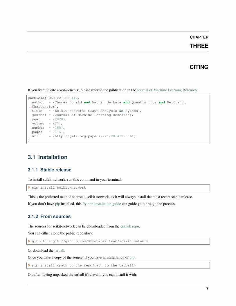
If you want to cite scikit-network, please refer to the publication in the Journal of Machine Learning Research:
@article{JMLR:v21:20-412,author = {Thomas Bonald and Nathan de Lara and Quentin Lutz and Bertrand
→˓Charpentier},title = {Scikit-network: Graph Analysis in Python},journal = {Journal of Machine Learning Research},year = {2020},volume = {21},number = {185},pages = {1-6},url = {http://jmlr.org/papers/v21/20-412.html}
}
3.1 Installation
3.1.1 Stable release
To install scikit-network, run this command in your terminal:
$ pip install scikit-network
This is the preferred method to install scikit-network, as it will always install the most recent stable release.
If you don’t have pip installed, this Python installation guide can guide you through the process.
3.1.2 From sources
The sources for scikit-network can be downloaded from the Github repo.
You can either clone the public repository:
$ git clone git://github.com/sknetwork-team/scikit-network
Or download the tarball.
Once you have a copy of the source, if you have an installation of pip:
$ pip install <path to the repo/path to the tarball>
Or, after having unpacked the tarball if relevant, you can install it with:
7
scikit-network Documentation, Release 0.23.1
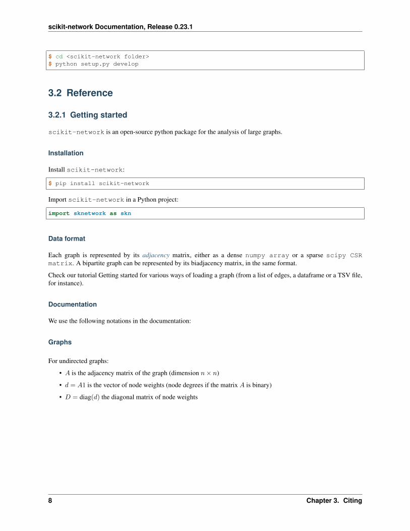
$ cd <scikit-network folder>$ python setup.py develop
3.2 Reference
3.2.1 Getting started
scikit-network is an open-source python package for the analysis of large graphs.
Installation
Install scikit-network:
$ pip install scikit-network
Import scikit-network in a Python project:
import sknetwork as skn
Data format
Each graph is represented by its adjacency matrix, either as a dense numpy array or a sparse scipy CSRmatrix. A bipartite graph can be represented by its biadjacency matrix, in the same format.
Check our tutorial Getting started for various ways of loading a graph (from a list of edges, a dataframe or a TSV file,for instance).
Documentation
We use the following notations in the documentation:
Graphs
For undirected graphs:
• 𝐴 is the adjacency matrix of the graph (dimension 𝑛× 𝑛)
• 𝑑 = 𝐴1 is the vector of node weights (node degrees if the matrix 𝐴 is binary)
• 𝐷 = diag(𝑑) the diagonal matrix of node weights
8 Chapter 3. Citing
scikit-network Documentation, Release 0.23.1
Digraphs
For directed graphs:
• 𝐴 is the adjacency matrix of the graph (dimension 𝑛× 𝑛)
• 𝑑+ = 𝐴1 and 𝑑− = 𝐴𝑇 1 are the vectors of out-weights and in-weights of nodes (out-degrees and in-degrees ifthe matrix 𝐴 is binary)
• 𝐷+ = diag(𝑑+) and 𝐷− = diag(𝑑−) are the diagonal matrices of out-weights and in-weights
Bigraphs
For bipartite graphs:
• 𝐵 is the biadjacency matrix of the graph (dimension 𝑛1 × 𝑛2)
• 𝑑1 = 𝐵1 and 𝑑2 = 𝐵𝑇 1 are the vectors of weights (rows and columns)
• 𝐷1 = diag(𝑑1) and 𝐷2 = diag(𝑑2) are the diagonal matrices of weights.
Notes
• Adjacency and biadjacency matrices have non-negative entries (the weights of the edges).
• Bipartite graphs are undirected but have a special structure that is exploited by some algorithms. These algo-rithms are identified with the prefix Bi.
3.2.2 Data
Tools for importing and exporting data.
Toy graphs
sknetwork.data.house(metadata: bool = False) → Union[scipy.sparse.csr.csr_matrix, sknet-work.utils.Bunch]
House graph.
• Undirected graph
• 5 nodes, 6 edges
Parameters metadata – If True, return a Bunch object with metadata.
Returns adjacency or graph – Adjacency matrix or graph with metadata (positions).
Return type Union[sparse.csr_matrix, Bunch]
3.2. Reference 9
scikit-network Documentation, Release 0.23.1
Example
>>> from sknetwork.data import house>>> adjacency = house()>>> adjacency.shape(5, 5)
sknetwork.data.bow_tie(metadata: bool = False) → Union[scipy.sparse.csr.csr_matrix, sknet-work.utils.Bunch]
Bow tie graph.
• Undirected graph
• 5 nodes, 6 edges
Parameters metadata – If True, return a Bunch object with metadata.
Returns adjacency or graph – Adjacency matrix or graph with metadata (positions).
Return type Union[sparse.csr_matrix, Bunch]
Example
>>> from sknetwork.data import bow_tie>>> adjacency = bow_tie()>>> adjacency.shape(5, 5)
sknetwork.data.karate_club(metadata: bool = False) → Union[scipy.sparse.csr.csr_matrix, sknet-work.utils.Bunch]
Karate club graph.
• Undirected graph
• 34 nodes, 78 edges
• 2 labels
Parameters metadata – If True, return a Bunch object with metadata.
Returns adjacency or graph – Adjacency matrix or graph with metadata (labels, positions).
Return type Union[sparse.csr_matrix, Bunch]
Example
>>> from sknetwork.data import karate_club>>> adjacency = karate_club()>>> adjacency.shape(34, 34)
10 Chapter 3. Citing
scikit-network Documentation, Release 0.23.1
References
Zachary’s karate club graph https://en.wikipedia.org/wiki/Zachary%27s_karate_club
sknetwork.data.miserables(metadata: bool = False) → Union[scipy.sparse.csr.csr_matrix, sknet-work.utils.Bunch]
Co-occurrence graph of the characters in the novel Les miserables by Victor Hugo.
• Undirected graph
• 77 nodes, 508 edges
• Names of characters
Parameters metadata – If True, return a Bunch object with metadata.
Returns adjacency or graph – Adjacency matrix or graph with metadata (names, positions).
Return type Union[sparse.csr_matrix, Bunch]
Example
>>> from sknetwork.data import miserables>>> adjacency = miserables()>>> adjacency.shape(77, 77)
sknetwork.data.painters(metadata: bool = False) → Union[scipy.sparse.csr.csr_matrix, sknet-work.utils.Bunch]
Graph of links between some famous painters on Wikipedia.
• Directed graph
• 14 nodes, 50 edges
• Names of painters
Parameters metadata – If True, return a Bunch object with metadata.
Returns adjacency or graph – Adjacency matrix or graph with metadata (names, positions).
Return type Union[sparse.csr_matrix, Bunch]
Example
>>> from sknetwork.data import painters>>> adjacency = painters()>>> adjacency.shape(14, 14)
sknetwork.data.star_wars(metadata: bool = False) → Union[scipy.sparse.csr.csr_matrix, sknet-work.utils.Bunch]
Bipartite graph connecting some Star Wars villains to the movies in which they appear.
• Bipartite graph
• 7 nodes (4 villains, 3 movies), 8 edges
• Names of villains and movies
3.2. Reference 11
scikit-network Documentation, Release 0.23.1
Parameters metadata – If True, return a Bunch object with metadata.
Returns biadjacency or graph – Biadjacency matrix or graph with metadata (names).
Return type Union[sparse.csr_matrix, Bunch]
Example
>>> from sknetwork.data import star_wars>>> biadjacency = star_wars()>>> biadjacency.shape(4, 3)
sknetwork.data.movie_actor(metadata: bool = False) → Union[scipy.sparse.csr.csr_matrix, sknet-work.utils.Bunch]
Bipartite graph connecting movies to some actors starring in them.
• Bipartite graph
• 31 nodes (15 movies, 16 actors), 42 edges
• 9 labels (rows)
• Names of movies (rows) and actors (columns)
• Names of movies production company (rows)
Parameters metadata – If True, return a Bunch object with metadata.
Returns biadjacency or graph – Biadjacency matrix or graph with metadata (names).
Return type Union[sparse.csr_matrix, Bunch]
Example
>>> from sknetwork.data import movie_actor>>> biadjacency = movie_actor()>>> biadjacency.shape(15, 16)
Models
sknetwork.data.linear_graph(n: int = 3, metadata: bool = False) →Union[scipy.sparse.csr.csr_matrix, sknetwork.utils.Bunch]
Linear graph (undirected).
Parameters
• n (int) – Number of nodes.
• metadata (bool) – If True, return a Bunch object with metadata.
Returns adjacency or graph – Adjacency matrix or graph with metadata (positions).
Return type Union[sparse.csr_matrix, Bunch]
12 Chapter 3. Citing
scikit-network Documentation, Release 0.23.1
Example
>>> from sknetwork.data import linear_graph>>> adjacency = linear_graph(5)>>> adjacency.shape(5, 5)
sknetwork.data.linear_digraph(n: int = 3, metadata: bool = False) →Union[scipy.sparse.csr.csr_matrix, sknetwork.utils.Bunch]
Linear graph (directed).
Parameters
• n (int) – Number of nodes.
• metadata (bool) – If True, return a Bunch object with metadata.
Returns adjacency or graph – Adjacency matrix or graph with metadata (positions).
Return type Union[sparse.csr_matrix, Bunch]
Example
>>> from sknetwork.data import linear_digraph>>> adjacency = linear_digraph(5)>>> adjacency.shape(5, 5)
sknetwork.data.cyclic_graph(n: int = 3, metadata: bool = False) →Union[scipy.sparse.csr.csr_matrix, sknetwork.utils.Bunch]
Cyclic graph (undirected).
Parameters
• n (int) – Number of nodes.
• metadata (bool) – If True, return a Bunch object with metadata.
Returns adjacency or graph – Adjacency matrix or graph with metadata (positions).
Return type Union[sparse.csr_matrix, Bunch]
Example
>>> from sknetwork.data import cyclic_graph>>> adjacency = cyclic_graph(5)>>> adjacency.shape(5, 5)
sknetwork.data.cyclic_digraph(n: int = 3, metadata: bool = False) →Union[scipy.sparse.csr.csr_matrix, sknetwork.utils.Bunch]
Cyclic graph (directed).
Parameters
• n (int) – Number of nodes.
• metadata (bool) – If True, return a Bunch object with metadata.
Returns adjacency or graph – Adjacency matrix or graph with metadata (positions).
3.2. Reference 13
scikit-network Documentation, Release 0.23.1
Return type Union[sparse.csr_matrix, Bunch]
Example
>>> from sknetwork.data import cyclic_digraph>>> adjacency = cyclic_digraph(5)>>> adjacency.shape(5, 5)
sknetwork.data.grid(n1: int = 10, n2: int = 10, metadata: bool = False) →Union[scipy.sparse.csr.csr_matrix, sknetwork.utils.Bunch]
Grid (undirected).
Parameters
• n1 (int) – Grid dimension.
• n2 (int) – Grid dimension.
• metadata (bool) – If True, return a Bunch object with metadata.
Returns adjacency or graph – Adjacency matrix or graph with metadata (positions).
Return type Union[sparse.csr_matrix, Bunch]
Example
>>> from sknetwork.data import grid>>> adjacency = grid(10, 5)>>> adjacency.shape(50, 50)
sknetwork.data.erdos_renyi(n: int = 20, p: float = 0.3, random_state: Optional[int] = None) →scipy.sparse.csr.csr_matrix
Erdos-Renyi graph.
Parameters
• n – Number of nodes.
• p – Probability of connection between nodes.
• random_state – Seed of the random generator (optional).
Returns adjacency – Adjacency matrix.
Return type sparse.csr_matrix
Example
>>> from sknetwork.data import erdos_renyi>>> adjacency = erdos_renyi(7)>>> adjacency.shape(7, 7)
14 Chapter 3. Citing
scikit-network Documentation, Release 0.23.1
References
Erdos, P., Rényi, A. (1959). On Random Graphs. Publicationes Mathematicae.
sknetwork.data.block_model(sizes: Iterable, p_in: Union[float, list, numpy.ndarray] = 0.2, p_out:float = 0.05, random_state: Optional[int] = None, metadata: bool =False)→ Union[scipy.sparse.csr.csr_matrix, sknetwork.utils.Bunch]
Stochastic block model.
Parameters
• sizes – Block sizes.
• p_in – Probability of connection within blocks.
• p_out – Probability of connection across blocks.
• random_state – Seed of the random generator (optional).
• metadata – If True, return a Bunch object with metadata.
Returns adjacency or graph – Adjacency matrix or graph with metadata (labels).
Return type Union[sparse.csr_matrix, Bunch]
Example
>>> from sknetwork.data import block_model>>> sizes = np.array([4, 5])>>> adjacency = block_model(sizes)>>> adjacency.shape(9, 9)
References
Airoldi, E., Blei, D., Feinberg, S., Xing, E. (2007). Mixed membership stochastic blockmodels. Journal ofMachine Learning Research.
sknetwork.data.albert_barabasi(n: int = 100, degree: int = 3, undirected: bool = True, seed:Optional[int] = None)→ scipy.sparse.csr.csr_matrix
Albert-Barabasi model.
Parameters
• n (int) – Number of nodes.
• degree (int) – Degree of incoming nodes (less than n).
• undirected (bool) – If True, return an undirected graph.
• seed – Seed of the random generator (optional).
Returns adjacency – Adjacency matrix.
Return type sparse.csr_matrix
3.2. Reference 15
scikit-network Documentation, Release 0.23.1
Example
>>> from sknetwork.data import albert_barabasi>>> adjacency = albert_barabasi(30, 3)>>> adjacency.shape(30, 30)
References
Albert, R., Barabási, L. (2002). Statistical mechanics of complex networks Reviews of Modern Physics.
sknetwork.data.watts_strogatz(n: int = 100, degree: int = 6, prob: float = 0.05,seed: Optional[int] = None, metadata: bool = False) →Union[scipy.sparse.csr.csr_matrix, sknetwork.utils.Bunch]
Watts-Strogatz model.
Parameters
• n – Number of nodes.
• degree – Initial degree of nodes.
• prob – Probability of edge modification.
• seed – Seed of the random generator (optional).
• metadata – If True, return a Bunch object with metadata.
Returns adjacency or graph – Adjacency matrix or graph with metadata (positions).
Return type Union[sparse.csr_matrix, Bunch]
Example
>>> from sknetwork.data import watts_strogatz>>> adjacency = watts_strogatz(30, 4, 0.02)>>> adjacency.shape(30, 30)
References
Watts, D., Strogatz, S. (1998). Collective dynamics of small-world networks, Nature.
Load
You can find some datasets on NetRep.
sknetwork.data.load_edge_list(file: str, directed: bool = False, bipartite: bool = False, weighted:Optional[bool] = None, named: Optional[bool] = None, com-ment: str = '%#', delimiter: Optional[str] = None, reindex: bool= True, fast_format: bool = True)→ sknetwork.utils.Bunch
Parse Tabulation-Separated, Comma-Separated or Space-Separated (or other) Values datasets in the form ofedge lists.
Parameters
• file (str) – The path to the dataset in TSV format
16 Chapter 3. Citing
scikit-network Documentation, Release 0.23.1
• directed (bool) – If True, considers the graph as directed.
• bipartite (bool) – If True, returns a biadjacency matrix of shape (n1, n2).
• weighted (Optional[bool]) – Retrieves the weights in the third field of the file. Nonemakes a guess based on the first lines.
• named (Optional[bool]) – Retrieves the names given to the nodes and renumbersthem. Returns an additional array. None makes a guess based on the first lines.
• comment (str) – Set of characters denoting lines to ignore.
• delimiter (str) – delimiter used in the file. None makes a guess
• reindex (bool) – If True and the graph nodes have numeric values, the size of the re-turned adjacency will be determined by the maximum of those values. Does not work forbipartite graphs.
• fast_format (bool) – If True, assumes that the file is well-formatted:
– no comments except for the header
– only 2 or 3 columns
– only int or float values
Returns graph
Return type Bunch
sknetwork.data.load_adjacency_list(file: str, bipartite: bool = False, comment: str = '%#', de-limiter: Optional[str] = None)→ sknetwork.utils.Bunch
Parse Tabulation-Separated, Comma-Separated or Space-Separated (or other) Values datasets in the form ofadjacency lists.
Parameters
• file (str) – The path to the dataset in TSV format
• bipartite (bool) – If True, returns a biadjacency matrix of shape (n1, n2).
• comment (str) – Set of characters denoting lines to ignore.
• delimiter (str) – delimiter used in the file. None makes a guess
Returns graph
Return type Bunch
sknetwork.data.load_graphml(file: str, weight_key: str = 'weight', max_string_size: int = 512) →sknetwork.utils.Bunch
Parse GraphML datasets.
Hyperedges and nested graphs are not supported.
Parameters
• file (str) – The path to the dataset
• weight_key (str) – The key to be used as a value for edge weights
• max_string_size (int) – The maximum size for string features of the data
Returns data – The dataset in a bunch with the adjacency as a CSR matrix.
Return type Bunch
3.2. Reference 17
scikit-network Documentation, Release 0.23.1
sknetwork.data.load_netset(dataset: Optional[str] = None, data_home: Optional[Union[str, path-lib.Path]] = None, verbose: bool = True)→ sknetwork.utils.Bunch
Load a dataset from the NetSet database.
Parameters
• dataset (str) – The name of the dataset (all low-case). Examples include ‘openflights’,‘cinema’ and ‘wikivitals’.
• data_home (str or pathlib.Path) – The folder to be used for dataset storage.
• verbose (bool) – Enable verbosity.
Returns graph
Return type Bunch
sknetwork.data.load_konect(dataset: str, data_home: Optional[Union[str, pathlib.Path]] = None,auto_numpy_bundle: bool = True, verbose: bool = True) → sknet-work.utils.Bunch
Load a dataset from the Konect database.
Parameters
• dataset (str) – The internal name of the dataset as specified on the Konect website (e.g.for the Zachary Karate club dataset, the corresponding name is 'ucidata-zachary').
• data_home (str or pathlib.Path) – The folder to be used for dataset storage
• auto_numpy_bundle (bool) – Denotes if the dataset should be stored in its defaultformat (False) or using Numpy files for faster subsequent access to the dataset (True).
• verbose (bool) – Enable verbosity.
Returns
graph –
An object with the following attributes:
• adjacency or biadjacency: the adjacency/biadjacency matrix for the dataset
• meta: a dictionary containing the metadata as specified by Konect
• each attribute specified by Konect (ent.* file)
Return type Bunch
Notes
An attribute meta of the Bunch class is used to store information about the dataset if present. In any case, metahas the attribute name which, if not given, is equal to the name of the dataset as passed to this function.
18 Chapter 3. Citing
scikit-network Documentation, Release 0.23.1
References
Kunegis, J. (2013, May). Konect: the Koblenz network collection. In Proceedings of the 22nd InternationalConference on World Wide Web (pp. 1343-1350).
sknetwork.data.convert_edge_list(edge_list: Union[numpy.ndarray, List[Tuple], List[List]], di-rected: bool = False, bipartite: bool = False, reindex:bool = True, named: Optional[bool] = None) → sknet-work.utils.Bunch
Turn an edge list into a Bunch.
Parameters
• edge_list (Union[np.ndarray, List[Tuple], List[List]]) – The edgelist to convert, given as a NumPy array of size (n, 2) or (n, 3) or a list of either lists or tuplesof length 2 or 3.
• directed (bool) – If True, considers the graph as directed.
• bipartite (bool) – If True, returns a biadjacency matrix of shape (n1, n2).
• reindex (bool) – If True and the graph nodes have numeric values, the size of the re-turned adjacency will be determined by the maximum of those values. Does not work forbipartite graphs.
• named (Optional[bool]) – Retrieves the names given to the nodes and renumbersthem. Returns an additional array. None makes a guess based on the first lines.
Returns graph
Return type Bunch
Save
sknetwork.data.save(folder: Union[str, pathlib.Path], data: Union[scipy.sparse.csr.csr_matrix, sknet-work.utils.Bunch])
Save a Bunch or a CSR matrix in the current directory to a collection of Numpy and Pickle files for fastersubsequent loads. Supported attribute types include sparse matrices, NumPy arrays, strings and Bunch.
Parameters
• folder (str or pathlib.Path) – The name to be used for the bundle folder
• data (Union[sparse.csr_matrix, Bunch]) – The data to save
Example
>>> from sknetwork.data import save>>> graph = Bunch()>>> graph.adjacency = sparse.csr_matrix(np.random.random((10, 10)) < 0.2)>>> graph.names = np.array(list('abcdefghij'))>>> save('random_data', graph)>>> 'random_data' in listdir('.')True
sknetwork.data.load(folder: Union[str, pathlib.Path])Load a Bunch from a previously created bundle from the current directory (inverse function of save).
Parameters folder (str) – The name used for the bundle folder
3.2. Reference 19
scikit-network Documentation, Release 0.23.1
Returns data – The original data
Return type Bunch
Example
>>> from sknetwork.data import save>>> graph = Bunch()>>> graph.adjacency = sparse.csr_matrix(np.random.random((10, 10)) < 0.2)>>> graph.names = np.array(list('abcdefghij'))>>> save('random_data', graph)>>> loaded_graph = load('random_data')>>> loaded_graph.names[0]'a'
3.2.3 Topology
Algorithms for the analysis of graph topology.
Structure
sknetwork.topology.connected_components(adjacency: scipy.sparse.csr.csr_matrix, connec-tion: str = 'weak')→ numpy.ndarray
Extract the connected components of the graph.
• Graphs
• Digraphs
Based on SciPy (scipy.sparse.csgraph.connected_components).
Parameters
• adjacency – Adjacency matrix of the graph.
• connection – Must be 'weak' (default) or 'strong'. The type of connection to usefor directed graphs.
Returns labels – Connected component of each node.
Return type np.ndarray
sknetwork.topology.largest_connected_component(adjacency:Union[scipy.sparse.csr.csr_matrix,numpy.ndarray], return_labels: bool =False)
Extract the largest connected component of a graph. Bipartite graphs are treated as undirected.
• Graphs
• Digraphs
• Bigraphs
Parameters
• adjacency – Adjacency or biadjacency matrix of the graph.
• return_labels (bool) – Whether to return the indices of the new nodes in the originalgraph.
20 Chapter 3. Citing
scikit-network Documentation, Release 0.23.1
Returns
• new_adjacency (sparse.csr_matrix) – Adjacency or biadjacency matrix of the largest con-nected component.
• indices (array or tuple of array) – Indices of the nodes in the original graph. For biadjacencymatrices, indices[0] corresponds to the rows and indices[1] to the columns.
class sknetwork.topology.CoreDecompositionK-core decomposition algorithm.
• Graphs
Variables
• labels_ (np.ndarray) – Core value of each node.
• core_value_ (int) – Maximum core value of the graph
Example
>>> from sknetwork.topology import CoreDecomposition>>> from sknetwork.data import karate_club>>> kcore = CoreDecomposition()>>> adjacency = karate_club()>>> kcore.fit(adjacency)>>> kcore.core_value_4
fit(adjacency: scipy.sparse.csr.csr_matrix)→ sknetwork.topology.kcore.CoreDecompositionK-core decomposition.
Parameters adjacency – Adjacency matrix of the graph.
Returns self
Return type CoreDecomposition
fit_transform(adjacency: scipy.sparse.csr.csr_matrix)Fit algorithm to the data and return the core value of each node. Same parameters as the fit method.
Returns Core value of the nodes.
Return type labels
sknetwork.topology.is_bipartite(adjacency: scipy.sparse.csr.csr_matrix, return_biadjacency:bool = False) → Union[bool, Tuple[bool, Op-tional[scipy.sparse.csr.csr_matrix], Optional[numpy.ndarray],Optional[numpy.ndarray]]]
Check whether an undirected graph is bipartite.
• Graphs
Parameters
• adjacency – Adjacency matrix of the graph (symmetric).
• return_biadjacency – If True, return a biadjacency matrix of the graph if bipartite.
Returns
• is_bipartite (bool) – A boolean denoting if the graph is bipartite.
3.2. Reference 21
scikit-network Documentation, Release 0.23.1
• biadjacency (sparse.csr_matrix) – A biadjacency matrix of the graph if bipartite (optional).
• rows (np.ndarray) – Index of rows in the original graph (optional).
• cols (np.ndarray) – Index of columns in the original graph (optional).
sknetwork.topology.is_acyclic(adjacency: scipy.sparse.csr.csr_matrix)→ boolCheck whether a graph has no cycle.
Parameters adjacency – Adjacency matrix of the graph.
Returns is_acyclic – A boolean with value True if the graph has no cycle and False otherwise
Return type bool
class sknetwork.topology.DAG(ordering: Optional[str] = None)Build a Directed Acyclic Graph from an adjacency.
• Graphs
• DiGraphs
Parameters ordering (str) – A method to sort the nodes.
• If None, the default order is the index.
• If 'degree', the nodes are sorted by ascending degree.
Variables
• indptr_ (np.ndarray) – Pointer index as for CSR format.
• indices_ (np.ndarray) – Indices as for CSR format.
fit(adjacency: scipy.sparse.csr.csr_matrix, sorted_nodes=None)Fit algorithm to the data.
Parameters
• adjacency – Adjacency matrix of the graph.
• sorted_nodes (np.ndarray) – An order on the nodes such that the DAG only con-tains edges (i, j) such that sorted_nodes[i] < sorted_nodes[j].
Counting
class sknetwork.topology.Triangles(parallelize: bool = False)Count the number of triangles in a graph, and evaluate the clustering coefficient.
• Graphs
Parameters parallelize – If True, use a parallel range while listing the triangles.
Variables
• n_triangles_ (int) – Number of triangles.
• clustering_coef_ (float) – Global clustering coefficient of the graph.
22 Chapter 3. Citing
scikit-network Documentation, Release 0.23.1
Example
>>> from sknetwork.data import karate_club>>> triangles = Triangles()>>> adjacency = karate_club()>>> triangles.fit_transform(adjacency)45
fit(adjacency: scipy.sparse.csr.csr_matrix)→ sknetwork.topology.triangles.TrianglesCount triangles.
Parameters adjacency – Adjacency matrix of the graph.
Returns self
Return type Triangles
fit_transform(adjacency: scipy.sparse.csr.csr_matrix)→ intFit algorithm to the data and return the number of triangles. Same parameters as the fit method.
Returns n_triangles_ – Number of triangles.
Return type int
class sknetwork.topology.Cliques(k: int)Clique counting algorithm.
• Graphs
Parameters k (int) – k value of cliques to list
Variables n_cliques_ (int) – Number of cliques
Example
>>> from sknetwork.data import karate_club>>> cliques = Cliques(k=3)>>> adjacency = karate_club()>>> cliques.fit_transform(adjacency)45
References
Danisch, M., Balalau, O., & Sozio, M. (2018, April). Listing k-cliques in sparse real-world graphs. In Proceed-ings of the 2018 World Wide Web Conference (pp. 589-598).
fit(adjacency: scipy.sparse.csr.csr_matrix)→ sknetwork.topology.kcliques.CliquesK-cliques count.
Parameters adjacency – Adjacency matrix of the graph.
Returns self
Return type Cliques
fit_transform(adjacency: scipy.sparse.csr.csr_matrix)→ intFit algorithm to the data and return the number of cliques. Same parameters as the fit method.
Returns n_cliques – Number of k-cliques.
3.2. Reference 23
scikit-network Documentation, Release 0.23.1
Return type int
Coloring
class sknetwork.topology.WeisfeilerLehman(max_iter: int = - 1)Weisfeiler-Lehman algorithm for coloring/labeling graphs in order to check similarity.
Parameters max_iter (int) – Maximum number of iterations. Negative value means until con-vergence.
Variables labels_ (np.ndarray) – Label of each node.
Example
>>> from sknetwork.topology import WeisfeilerLehman>>> from sknetwork.data import house>>> weisfeiler_lehman = WeisfeilerLehman()>>> adjacency = house()>>> labels = weisfeiler_lehman.fit_transform(adjacency)>>> labelsarray([0, 2, 1, 1, 2], dtype=int32)
References
• Douglas, B. L. (2011). The Weisfeiler-Lehman Method and Graph Isomorphism Testing.
• Shervashidze, N., Schweitzer, P., van Leeuwen, E. J., Melhorn, K., Borgwardt, K. M. (2011) Weisfeiler-Lehman graph kernels. Journal of Machine Learning Research 12, 2011.
fit(adjacency: Union[scipy.sparse.csr.csr_matrix, numpy.ndarray]) → sknet-work.topology.weisfeiler_lehman.WeisfeilerLehmanFit algorithm to the data.
Parameters adjacency (Union[sparse.csr_matrix, np.ndarray]) – Adja-cency matrix of the graph.
Returns self
Return type WeisfeilerLehman
fit_transform(adjacency: Union[scipy.sparse.csr.csr_matrix, numpy.ndarray])→ numpy.ndarrayFit algorithm to the data and return the labels. Same parameters as the fit method.
Returns labels – Labels.
Return type np.ndarray
24 Chapter 3. Citing
scikit-network Documentation, Release 0.23.1
Similarity
sknetwork.topology.are_isomorphic(adjacency1: scipy.sparse.csr.csr_matrix, adjacency2:scipy.sparse.csr.csr_matrix, max_iter: int = - 1)→ bool
Weisfeiler-Lehman isomorphism test. If the test is False, the graphs cannot be isomorphic, otherwise, they mightbe.
Parameters
• adjacency1 – First adjacency matrix.
• adjacency2 – Second adjacency matrix.
• max_iter (int) – Maximum number of coloring iterations. Negative value means untilconvergence.
Returns test_result
Return type bool
Example
>>> from sknetwork.topology import are_isomorphic>>> from sknetwork.data import house>>> adjacency_1 = house()>>> adjacency_2 = house()>>> are_isomorphic(adjacency_1, adjacency_2)True
References
• Douglas, B. L. (2011). The Weisfeiler-Lehman Method and Graph Isomorphism Testing.
• Shervashidze, N., Schweitzer, P., van Leeuwen, E. J., Melhorn, K., Borgwardt, K. M. (2011) Weisfeiler-Lehman graph kernels. Journal of Machine Learning Research 12, 2011.
3.2.4 Path
Standard algorithms related to graph traversal.
Most algorithms are adapted from SciPy.
Shortest path
sknetwork.path.distance(adjacency: scipy.sparse.csr.csr_matrix, sources: Optional[Union[int, Iter-able]] = None, method: str = 'D', return_predecessors: bool = False, un-weighted: bool = False, n_jobs: Optional[int] = None)
Compute distances between nodes.
• Graphs
• Digraphs
Based on SciPy (scipy.sparse.csgraph.shortest_path)
Parameters
• adjacency – The adjacency matrix of the graph
3.2. Reference 25
scikit-network Documentation, Release 0.23.1
• sources – If specified, only compute the paths for the points at the given indices. Will notwork with method =='FW'.
• method – The method to be used.
– 'D' (Dijkstra),
– 'BF' (Bellman-Ford),
– 'J' (Johnson).
• return_predecessors – If True, the size predecessor matrix is returned
• unweighted – If True, the weights of the edges are ignored
• n_jobs – If an integer value is given, denotes the number of workers to use (-1 means themaximum number will be used). If None, no parallel computations are made.
Returns
• dist_matrix (np.ndarray) – The matrix of distances between graph nodes.dist_matrix[i,j] gives the shortest distance from point i to point j along thegraph. If no path exists between nodes i and j, then dist_matrix[i, j] =np.inf.
• predecessors (np.ndarray, optional) – Returned only if return_predecessors ==True. The matrix of predecessors, which can be used to reconstruct the shortest paths.Row i of the predecessor matrix contains information on the shortest paths from point i:each entry predecessors[i, j] gives the index of the previous node in the path frompoint i to point j. If no path exists between nodes i and j, then predecessors[i, j]= -9999.
Examples
>>> from sknetwork.data import cyclic_digraph>>> adjacency = cyclic_digraph(3)>>> distance(adjacency, sources=0)array([0., 1., 2.])>>> distance(adjacency, sources=0, return_predecessors=True)(array([0., 1., 2.]), array([-9999, 0, 1]))
sknetwork.path.shortest_path(adjacency: scipy.sparse.csr.csr_matrix, sources: Union[int, Iter-able], targets: Union[int, Iterable], method: str = 'D', unweighted:bool = False, n_jobs: Optional[int] = None)
Compute the shortest paths in the graph.
• Graphs
• Digraphs
Parameters
• adjacency – The adjacency matrix of the graph
• sources (int or iterable) – Sources nodes.
• targets (int or iterable) – Target nodes.
• method – The method to be used.
– 'D' (Dijkstra),
– 'BF' (Bellman-Ford),
26 Chapter 3. Citing
scikit-network Documentation, Release 0.23.1
– 'J' (Johnson).
• unweighted – If True, the weights of the edges are ignored
• n_jobs – If an integer value is given, denotes the number of workers to use (-1 means themaximum number will be used). If None, no parallel computations are made.
Returns paths – If single source and single target, return a list containing the nodes on the pathfrom source to target. If multiple sources or multiple targets, return a list of paths as lists. Anempty list means that the path does not exist.
Return type list
Examples
>>> from sknetwork.data import linear_digraph>>> adjacency = linear_digraph(3)>>> shortest_path(adjacency, 0, 2)[0, 1, 2]>>> shortest_path(adjacency, 2, 0)[]>>> shortest_path(adjacency, 0, [1, 2])[[0, 1], [0, 1, 2]]>>> shortest_path(adjacency, [0, 1], 2)[[0, 1, 2], [1, 2]]
Summary of the different methods and their worst-case complexity for 𝑛 nodes and 𝑚 edges (for the all-pairs problem):
Method Worst-case time complexity RemarksDijkstra 𝑂(𝑛2 log 𝑛 + 𝑛𝑚) For use on graphs with positive weights onlyBellman-Ford 𝑂(𝑛𝑚) For use on graphs without negative-weight cycles onlyJohnson 𝑂(𝑛2 log 𝑛 + 𝑛𝑚)
Search
sknetwork.path.breadth_first_search(adjacency: scipy.sparse.csr.csr_matrix, source: int, re-turn_predecessors: bool = True)
Breadth-first ordering starting with specified node.
• Graphs
• Digraphs
Based on SciPy (scipy.sparse.csgraph.breadth_first_order)
Parameters
• adjacency – The adjacency matrix of the graph
• source (int) – The node from which to start the ordering
• return_predecessors (bool) – If True, the size predecessor matrix is returned
Returns
• node_array (np.ndarray) – The breadth-first list of nodes, starting with specified node. Thelength of node_array is the number of nodes reachable from the specified node.
3.2. Reference 27

scikit-network Documentation, Release 0.23.1
• predecessors (np.ndarray) – Returned only if return_predecessors == True.The list of predecessors of each node in a breadth-first tree. If node i is in the tree, thenits parent is given by predecessors[i]. If node i is not in the tree (and for the parentnode) then predecessors[i] = -9999.
sknetwork.path.depth_first_search(adjacency: scipy.sparse.csr.csr_matrix, source: int, re-turn_predecessors: bool = True)
Depth-first ordering starting with specified node.
• Graphs
• Digraphs
Based on SciPy (scipy.sparse.csgraph.depth_first_order)
Parameters
• adjacency – The adjacency matrix of the graph
• source – The node from which to start the ordering
• return_predecessors – If True, the size predecessor matrix is returned
Returns
• node_array (np.ndarray) – The depth-first list of nodes, starting with specified node. Thelength of node_array is the number of nodes reachable from the specified node.
• predecessors (np.ndarray) – Returned only if return_predecessors == True.The list of predecessors of each node in a depth-first tree. If node i is in the tree, thenits parent is given by predecessors[i]. If node i is not in the tree (and for the parentnode) then predecessors[i] = -9999.
Metrics
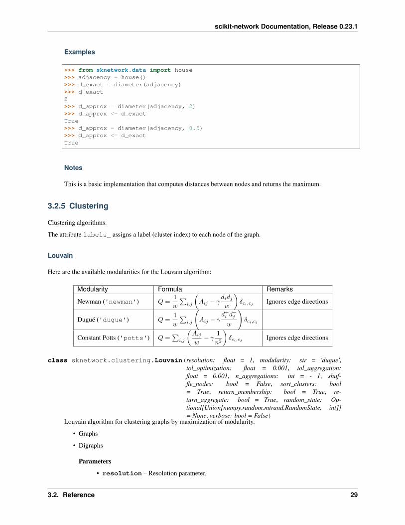
sknetwork.path.diameter(adjacency: Union[scipy.sparse.csr.csr_matrix, numpy.ndarray], n_sources:Optional[Union[int, float]] = None, n_jobs: Optional[int] = None)→ int
Lower bound on the diameter of a graph which is the length of the longest shortest path between two nodes.
Parameters
• adjacency – Adjacency matrix of the graph.
• n_sources – Number of node sources to use for approximation.
– If None, compute exact diameter.
– If int, sample n_sample source nodes at random.
– If float, sample (n_samples * n) source nodes at random.
• n_jobs – If an integer value is given, denotes the number of workers to use (-1 means themaximum number will be used). If None, no parallel computations are made.
Returns diameter
Return type int
28 Chapter 3. Citing
scikit-network Documentation, Release 0.23.1
Examples
>>> from sknetwork.data import house>>> adjacency = house()>>> d_exact = diameter(adjacency)>>> d_exact2>>> d_approx = diameter(adjacency, 2)>>> d_approx <= d_exactTrue>>> d_approx = diameter(adjacency, 0.5)>>> d_approx <= d_exactTrue
Notes
This is a basic implementation that computes distances between nodes and returns the maximum.
3.2.5 Clustering
Clustering algorithms.
The attribute labels_ assigns a label (cluster index) to each node of the graph.
Louvain
Here are the available modularities for the Louvain algorithm:
Modularity Formula Remarks
Newman ('newman') 𝑄 =1
𝑤
∑𝑖,𝑗
(𝐴𝑖𝑗 − 𝛾
𝑑𝑖𝑑𝑗𝑤
)𝛿𝑐𝑖,𝑐𝑗 Ignores edge directions
Dugué ('dugue') 𝑄 =1
𝑤
∑𝑖,𝑗
(𝐴𝑖𝑗 − 𝛾
𝑑+𝑖 𝑑−𝑗
𝑤
)𝛿𝑐𝑖,𝑐𝑗
Constant Potts ('potts') 𝑄 =∑
𝑖,𝑗
(𝐴𝑖𝑗
𝑤− 𝛾
1
𝑛2
)𝛿𝑐𝑖,𝑐𝑗 Ignores edge directions
class sknetwork.clustering.Louvain(resolution: float = 1, modularity: str = 'dugue',tol_optimization: float = 0.001, tol_aggregation:float = 0.001, n_aggregations: int = - 1, shuf-fle_nodes: bool = False, sort_clusters: bool= True, return_membership: bool = True, re-turn_aggregate: bool = True, random_state: Op-tional[Union[numpy.random.mtrand.RandomState, int]]= None, verbose: bool = False)
Louvain algorithm for clustering graphs by maximization of modularity.
• Graphs
• Digraphs
Parameters
• resolution – Resolution parameter.
3.2. Reference 29
scikit-network Documentation, Release 0.23.1
• modularity (str) – Which objective function to maximize. Can be 'dugue','newman' or 'potts'.
• tol_optimization – Minimum increase in the objective function to enter a new opti-mization pass.
• tol_aggregation – Minimum increase in the objective function to enter a new aggre-gation pass.
• n_aggregations – Maximum number of aggregations. A negative value is interpretedas no limit.
• shuffle_nodes – Enables node shuffling before optimization.
• sort_clusters – If True, sort labels in decreasing order of cluster size.
• return_membership – If True, return the membership matrix of nodes to each cluster(soft clustering).
• return_aggregate – If True, return the adjacency matrix of the graph between clus-ters.
• random_state – Random number generator or random seed. If None, numpy.random isused.
• verbose – Verbose mode.
Variables
• labels_ (np.ndarray) – Label of each node.
• membership_ (sparse.csr_matrix) – Membership matrix.
• adjacency_ (sparse.csr_matrix) – Adjacency matrix between clusters.
Example
>>> from sknetwork.clustering import Louvain>>> from sknetwork.data import karate_club>>> louvain = Louvain()>>> adjacency = karate_club()>>> labels = louvain.fit_transform(adjacency)>>> len(set(labels))4
References
• Blondel, V. D., Guillaume, J. L., Lambiotte, R., & Lefebvre, E. (2008). Fast unfolding of communities inlarge networks. Journal of statistical mechanics: theory and experiment, 2008
• Dugué, N., & Perez, A. (2015). Directed Louvain: maximizing modularity in directed networks (Doctoraldissertation, Université d’Orléans).
• Traag, V. A., Van Dooren, P., & Nesterov, Y. (2011). Narrow scope for resolution-limit-free communitydetection. Physical Review E, 84(1), 016114.
fit(adjacency: Union[scipy.sparse.csr.csr_matrix, numpy.ndarray]) → sknet-work.clustering.louvain.LouvainFit algorithm to the data.
30 Chapter 3. Citing
scikit-network Documentation, Release 0.23.1
Parameters adjacency – Adjacency matrix of the graph.
Returns self
Return type Louvain
fit_transform(*args, **kwargs)→ numpy.ndarrayFit algorithm to the data and return the labels. Same parameters as the fit method.
Returns labels – Labels.
Return type np.ndarray
class sknetwork.clustering.BiLouvain(resolution: float = 1, modularity: str = 'dugue',tol_optimization: float = 0.001, tol_aggregation:float = 0.001, n_aggregations: int = - 1, shuf-fle_nodes: bool = False, sort_clusters: bool= True, return_membership: bool = True, re-turn_aggregate: bool = True, random_state: Op-tional[Union[numpy.random.mtrand.RandomState,int]] = None, verbose: bool = False)
BiLouvain algorithm for the clustering of bipartite graphs.
• Bigraphs
Parameters
• resolution – Resolution parameter.
• modularity (str) – Which objective function to maximize. Can be 'dugue','newman' or 'potts'.
• tol_optimization – Minimum increase in the objective function to enter a new opti-mization pass.
• tol_aggregation – Minimum increase in the objective function to enter a new aggre-gation pass.
• n_aggregations – Maximum number of aggregations. A negative value is interpretedas no limit.
• shuffle_nodes – Enables node shuffling before optimization.
• sort_clusters – If True, sort labels in decreasing order of cluster size.
• return_membership – If True, return the membership matrix of nodes to each cluster(soft clustering).
• return_aggregate – If True, return the biadjacency matrix of the graph between clus-ters.
• random_state – Random number generator or random seed. If None, numpy.random isused.
• verbose – Verbose mode.
Variables
• labels_ (np.ndarray) – Labels of the rows.
• labels_row_ (np.ndarray) – Labels of the rows (copy of labels_).
• labels_col_ (np.ndarray) – Labels of the columns.
• membership_row_ (sparse.csr_matrix) – Membership matrix of the rows (copyof membership_).
3.2. Reference 31
scikit-network Documentation, Release 0.23.1
• membership_col_ (sparse.csr_matrix) – Membership matrix of the columns.Only valid if cluster_both = True.
• biadjacency_ (sparse.csr_matrix) – Biadjacency matrix of the aggregate graphbetween clusters.
Example
>>> from sknetwork.clustering import BiLouvain>>> from sknetwork.data import movie_actor>>> bilouvain = BiLouvain()>>> biadjacency = movie_actor()>>> labels = bilouvain.fit_transform(biadjacency)>>> len(labels)15
fit(biadjacency: Union[scipy.sparse.csr.csr_matrix, numpy.ndarray]) → sknet-work.clustering.louvain.BiLouvainApply the Louvain algorithm to the corresponding directed graph, with adjacency matrix:
𝐴 =
[0 𝐵0 0
]where 𝐵 is the input (biadjacency matrix).
Parameters biadjacency – Biadjacency matrix of the graph.
Returns self
Return type BiLouvain
fit_transform(*args, **kwargs)→ numpy.ndarrayFit algorithm to the data and return the labels. Same parameters as the fit method.
Returns labels – Labels.
Return type np.ndarray
Propagation
class sknetwork.clustering.PropagationClustering(n_iter: int = 5, node_order: str= 'decreasing', weighted: bool =True, sort_clusters: bool = True, re-turn_membership: bool = True, re-turn_aggregate: bool = True)
Clustering by label propagation.
• Graphs
• Digraphs
Parameters
• n_iter (int) – Maximum number of iterations (-1 for infinity).
• node_order (str) –
– ‘random’: node labels are updated in random order.
– ’increasing’: node labels are updated by increasing order of weight.
32 Chapter 3. Citing
scikit-network Documentation, Release 0.23.1
– ’decreasing’: node labels are updated by decreasing order of weight.
– Otherwise, node labels are updated by index order.
• weighted (bool) – If True, the vote of each neighbor is proportional to the edge weight.Otherwise, all votes have weight 1.
• sort_clusters – If True, sort labels in decreasing order of cluster size.
• return_membership – If True, return the membership matrix of nodes to each cluster(soft clustering).
• return_aggregate – If True, return the adjacency matrix of the graph between clus-ters.
Variables
• labels_ (np.ndarray) – Label of each node.
• membership_ (sparse.csr_matrix) – Membership matrix (columns = labels).
Example
>>> from sknetwork.clustering import PropagationClustering>>> from sknetwork.data import karate_club>>> propagation = PropagationClustering()>>> graph = karate_club(metadata=True)>>> adjacency = graph.adjacency>>> labels = propagation.fit_transform(adjacency)>>> len(set(labels))2
References
Raghavan, U. N., Albert, R., & Kumara, S. (2007). Near linear time algorithm to detect community structuresin large-scale networks. Physical review E, 76(3), 036106.
fit(adjacency: Union[scipy.sparse.csr.csr_matrix, numpy.ndarray]) → sknet-work.clustering.propagation_clustering.PropagationClusteringClustering by label propagation.
Parameters adjacency – Adjacency matrix of the graph.
Returns self
Return type PropagationClustering
fit_transform(*args, **kwargs)→ numpy.ndarrayFit algorithm to the data and return the labels. Same parameters as the fit method.
Returns labels – Labels.
Return type np.ndarray
score(label: int)Classification scores for a given label.
Parameters label (int) – The label index of the class.
Returns scores – Classification scores of shape (number of nodes,).
Return type np.ndarray
3.2. Reference 33
scikit-network Documentation, Release 0.23.1
class sknetwork.clustering.BiPropagationClustering(n_iter: int = 5, node_order: str= 'decreasing', weighted: bool =True, sort_clusters: bool = True,return_membership: bool = True,return_aggregate: bool = True)
Clustering by label propagation in bipartite graphs.
• Bigraphs
Parameters
• n_iter – Maximum number of iteration (-1 for infinity).
• sort_clusters – If True, sort labels in decreasing order of cluster size.
• return_membership – If True, return the membership matrix of nodes to each cluster(soft clustering).
• return_aggregate – If True, return the biadjacency matrix of the graph between clus-ters.
Variables
• labels_ (np.ndarray) – Label of each row.
• labels_row_ (np.ndarray) – Label of each row (copy of labels_).
• labels_col_ (np.ndarray) – Label of each column.
• membership_ (sparse.csr_matrix) – Membership matrix of rows.
• membership_row_ (sparse.csr_matrix) – Membership matrix of rows (copy ofmembership_).
• membership_col_ (sparse.csr_matrix) – Membership matrix of columns.
Example
>>> from sknetwork.clustering import BiPropagationClustering>>> from sknetwork.data import movie_actor>>> bipropagation = BiPropagationClustering()>>> graph = movie_actor(metadata=True)>>> biadjacency = graph.biadjacency>>> len(bipropagation.fit_transform(biadjacency))15>>> len(bipropagation.labels_col_)16
fit(biadjacency: Union[scipy.sparse.csr.csr_matrix, numpy.ndarray]) → sknet-work.clustering.propagation_clustering.BiPropagationClusteringClustering.
Parameters biadjacency – Biadjacency matrix of the graph.
Returns self
Return type BiPropagationClustering
fit_transform(*args, **kwargs)→ numpy.ndarrayFit algorithm to the data and return the labels. Same parameters as the fit method.
Returns labels – Labels.
34 Chapter 3. Citing
scikit-network Documentation, Release 0.23.1
Return type np.ndarray
score(label: int)Classification scores for a given label.
Parameters label (int) – The label index of the class.
Returns scores – Classification scores of shape (number of nodes,).
Return type np.ndarray
K-Means
class sknetwork.clustering.KMeans(n_clusters: int = 8, embedding_method:sknetwork.embedding.base.BaseEmbedding =GSVD(n_components=10, regularization=None, rela-tive_regularization=True, factor_row=0.5, factor_col=0.5,factor_singular=0.0, normalized=True, solver='auto'),sort_clusters: bool = True, return_membership: bool =True, return_aggregate: bool = True)
K-means applied in the embedding space.
• Graphs
• Digraphs
Parameters
• n_clusters – Number of desired clusters.
• embedding_method – Embedding method (default = GSVD in dimension 10, projectedon the unit sphere).
• sort_clusters – If True, sort labels in decreasing order of cluster size.
• return_membership – If True, return the membership matrix of nodes to each cluster(soft clustering).
• return_aggregate – If True, return the adjacency matrix of the graph between clus-ters.
Variables
• labels_ (np.ndarray) – Label of each node.
• membership_ (sparse.csr_matrix) – Membership matrix.
• adjacency_ (sparse.csr_matrix) – Adjacency matrix between clusters.
Example
>>> from sknetwork.clustering import KMeans>>> from sknetwork.data import karate_club>>> kmeans = KMeans(n_clusters=3)>>> adjacency = karate_club()>>> labels = kmeans.fit_transform(adjacency)>>> len(set(labels))3
3.2. Reference 35
scikit-network Documentation, Release 0.23.1
fit(adjacency: Union[scipy.sparse.csr.csr_matrix, numpy.ndarray]) → sknet-work.clustering.kmeans.KMeansApply embedding method followed by K-means.
Parameters adjacency – Adjacency matrix of the graph.
Returns self
Return type KMeans
fit_transform(*args, **kwargs)→ numpy.ndarrayFit algorithm to the data and return the labels. Same parameters as the fit method.
Returns labels – Labels.
Return type np.ndarray
class sknetwork.clustering.BiKMeans(n_clusters: int = 2, embedding_method: sknet-work.embedding.base.BaseBiEmbedding =GSVD(n_components=10, regularization=None,relative_regularization=True, factor_row=0.5, fac-tor_col=0.5, factor_singular=0.0, normalized=True,solver='auto'), co_cluster: bool = False, sort_clusters:bool = True, return_membership: bool = True, re-turn_aggregate: bool = True)
KMeans clustering of bipartite graphs applied in the embedding space.
• Bigraphs
Parameters
• n_clusters – Number of clusters.
• embedding_method – Embedding method (default = GSVD in dimension 10, projectedon the unit sphere).
• co_cluster – If True, co-cluster rows and columns (default = False).
• sort_clusters – If True, sort labels in decreasing order of cluster size.
• return_membership – If True, return the membership matrix of nodes to each cluster(soft clustering).
• return_aggregate – If True, return the biadjacency matrix of the graph between clus-ters.
Variables
• labels_ (np.ndarray) – Labels of the rows.
• labels_row_ (np.ndarray) – Labels of the rows (copy of labels_).
• labels_col_ (np.ndarray) – Labels of the columns. Only valid if co_cluster = True.
• membership_ (sparse.csr_matrix) – Membership matrix of the rows.
• membership_row_ (sparse.csr_matrix) – Membership matrix of the rows (copyof membership_).
• membership_col_ (sparse.csr_matrix) – Membership matrix of the columns.Only valid if co_cluster = True.
• biadjacency_ (sparse.csr_matrix) – Biadjacency matrix of the graph betweenclusters.
36 Chapter 3. Citing
scikit-network Documentation, Release 0.23.1
Example
>>> from sknetwork.clustering import BiKMeans>>> from sknetwork.data import movie_actor>>> bikmeans = BiKMeans()>>> biadjacency = movie_actor()>>> labels = bikmeans.fit_transform(biadjacency)>>> len(labels)15
fit(biadjacency: Union[scipy.sparse.csr.csr_matrix, numpy.ndarray]) → sknet-work.clustering.kmeans.BiKMeansApply embedding method followed by clustering to the graph.
Parameters biadjacency – Biadjacency matrix of the graph.
Returns self
Return type BiKMeans
fit_transform(*args, **kwargs)→ numpy.ndarrayFit algorithm to the data and return the labels. Same parameters as the fit method.
Returns labels – Labels.
Return type np.ndarray
Metrics
sknetwork.clustering.modularity(adjacency: Union[scipy.sparse.csr.csr_matrix,numpy.ndarray], labels: numpy.ndarray, weights: Union[str,numpy.ndarray] = 'degree', weights_in: Union[str,numpy.ndarray] = 'degree', resolution: float = 1, return_all:bool = False)→ Union[float, Tuple[float, float, float]]
Modularity of a clustering (node partition).
• Graphs
• Digraphs
The modularity of a clustering is
𝑄 =1
𝑤
∑𝑖,𝑗
(𝐴𝑖𝑗 − 𝛾
𝑑𝑖𝑑𝑗𝑤
)𝛿𝑐𝑖,𝑐𝑗 for graphs,
𝑄 =1
𝑤
∑𝑖,𝑗
(𝐴𝑖𝑗 − 𝛾
𝑑+𝑖 𝑑−𝑗
𝑤
)𝛿𝑐𝑖,𝑐𝑗 for digraphs,
where
• 𝑐𝑖 is the cluster of node 𝑖,
• 𝑑𝑖 is the weight of node 𝑖,
• 𝑑+𝑖 , 𝑑−𝑖 are the out-weight, in-weight of node 𝑖 (for digraphs),
• 𝑤 = 1𝑇𝐴1 is the total weight,
• 𝛿 is the Kronecker symbol,
• 𝛾 ≥ 0 is the resolution parameter.
3.2. Reference 37
scikit-network Documentation, Release 0.23.1
Parameters
• adjacency – Adjacency matrix of the graph.
• labels – Labels of nodes, vector of size 𝑛 .
• weights – Weights of nodes. 'degree' (default), 'uniform' or custom weights.
• weights_in – In-weights of nodes. None (default), 'degree', 'uniform' or customweights. If None, taken equal to weights.
• resolution – Resolution parameter (default = 1).
• return_all – If True, return modularity, fit, diversity.
Returns
• modularity (float)
• fit (float, optional)
• diversity (float, optional)
Example
>>> from sknetwork.clustering import modularity>>> from sknetwork.data import house>>> adjacency = house()>>> labels = np.array([0, 0, 1, 1, 0])>>> np.round(modularity(adjacency, labels), 2)0.11
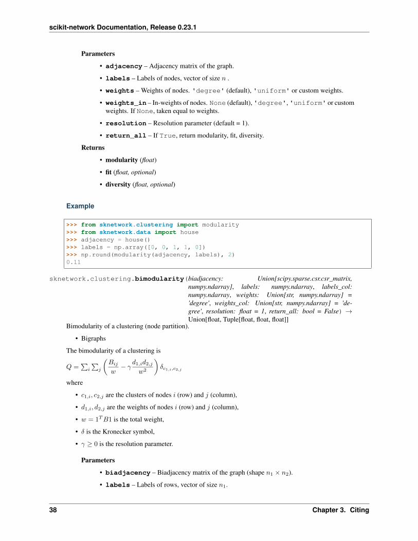
sknetwork.clustering.bimodularity(biadjacency: Union[scipy.sparse.csr.csr_matrix,numpy.ndarray], labels: numpy.ndarray, labels_col:numpy.ndarray, weights: Union[str, numpy.ndarray] ='degree', weights_col: Union[str, numpy.ndarray] = 'de-gree', resolution: float = 1, return_all: bool = False) →Union[float, Tuple[float, float, float]]
Bimodularity of a clustering (node partition).
• Bigraphs
The bimodularity of a clustering is
𝑄 =∑
𝑖
∑𝑗
(𝐵𝑖𝑗
𝑤− 𝛾
𝑑1,𝑖𝑑2,𝑗𝑤2
)𝛿𝑐1,𝑖,𝑐2,𝑗
where
• 𝑐1,𝑖, 𝑐2,𝑗 are the clusters of nodes 𝑖 (row) and 𝑗 (column),
• 𝑑1,𝑖, 𝑑2,𝑗 are the weights of nodes 𝑖 (row) and 𝑗 (column),
• 𝑤 = 1𝑇𝐵1 is the total weight,
• 𝛿 is the Kronecker symbol,
• 𝛾 ≥ 0 is the resolution parameter.
Parameters
• biadjacency – Biadjacency matrix of the graph (shape 𝑛1 × 𝑛2).
• labels – Labels of rows, vector of size 𝑛1.
38 Chapter 3. Citing
scikit-network Documentation, Release 0.23.1
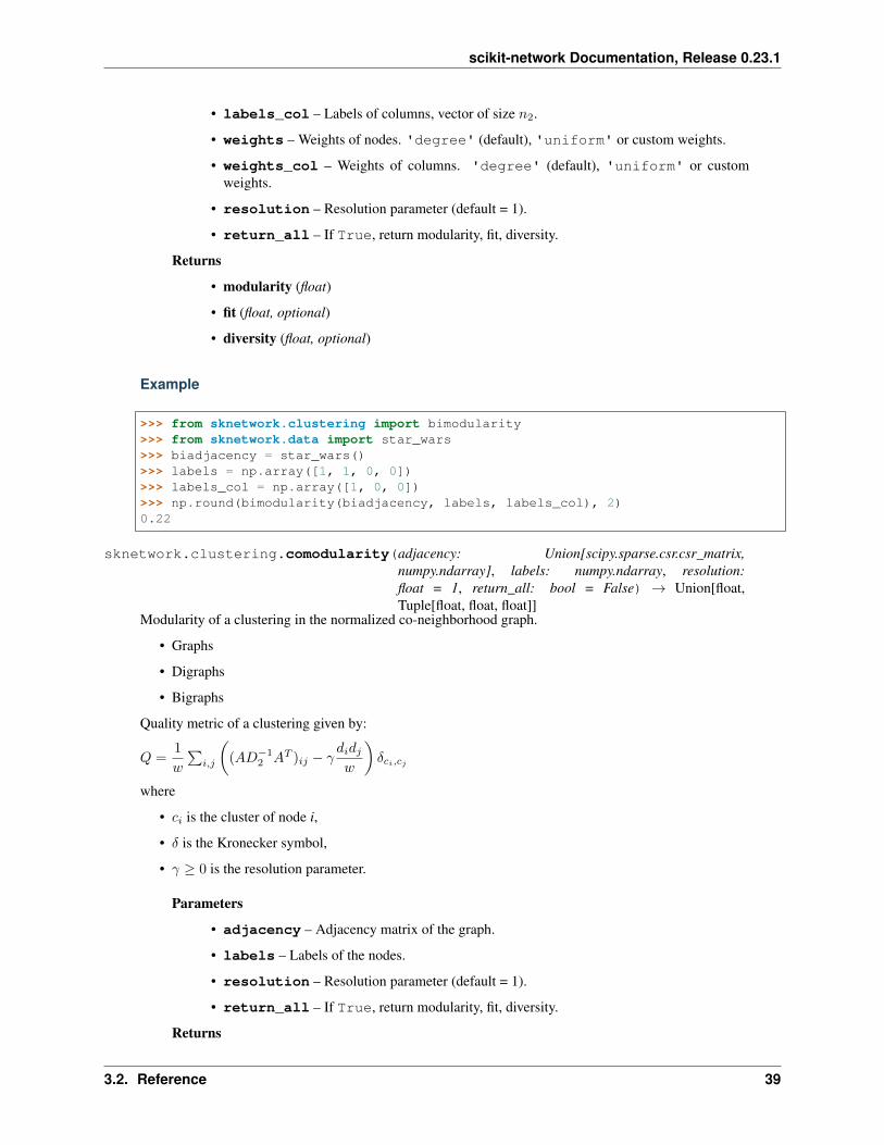
• labels_col – Labels of columns, vector of size 𝑛2.
• weights – Weights of nodes. 'degree' (default), 'uniform' or custom weights.
• weights_col – Weights of columns. 'degree' (default), 'uniform' or customweights.
• resolution – Resolution parameter (default = 1).
• return_all – If True, return modularity, fit, diversity.
Returns
• modularity (float)
• fit (float, optional)
• diversity (float, optional)
Example
>>> from sknetwork.clustering import bimodularity>>> from sknetwork.data import star_wars>>> biadjacency = star_wars()>>> labels = np.array([1, 1, 0, 0])>>> labels_col = np.array([1, 0, 0])>>> np.round(bimodularity(biadjacency, labels, labels_col), 2)0.22
sknetwork.clustering.comodularity(adjacency: Union[scipy.sparse.csr.csr_matrix,numpy.ndarray], labels: numpy.ndarray, resolution:float = 1, return_all: bool = False) → Union[float,Tuple[float, float, float]]
Modularity of a clustering in the normalized co-neighborhood graph.
• Graphs
• Digraphs
• Bigraphs
Quality metric of a clustering given by:
𝑄 =1
𝑤
∑𝑖,𝑗
((𝐴𝐷−1
2 𝐴𝑇 )𝑖𝑗 − 𝛾𝑑𝑖𝑑𝑗𝑤
)𝛿𝑐𝑖,𝑐𝑗
where
• 𝑐𝑖 is the cluster of node i,
• 𝛿 is the Kronecker symbol,
• 𝛾 ≥ 0 is the resolution parameter.
Parameters
• adjacency – Adjacency matrix of the graph.
• labels – Labels of the nodes.
• resolution – Resolution parameter (default = 1).
• return_all – If True, return modularity, fit, diversity.
Returns
3.2. Reference 39
scikit-network Documentation, Release 0.23.1
• modularity (float)
• fit (float, optional)
• diversity (float, optional)
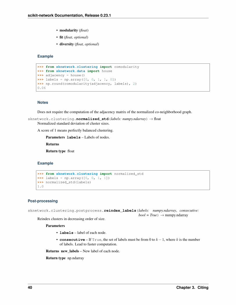
Example
>>> from sknetwork.clustering import comodularity>>> from sknetwork.data import house>>> adjacency = house()>>> labels = np.array([0, 0, 1, 1, 0])>>> np.round(comodularity(adjacency, labels), 2)0.06
Notes
Does not require the computation of the adjacency matrix of the normalized co-neighborhood graph.
sknetwork.clustering.normalized_std(labels: numpy.ndarray)→ floatNormalized standard deviation of cluster sizes.
A score of 1 means perfectly balanced clustering.
Parameters labels – Labels of nodes.
Returns
Return type float
Example
>>> from sknetwork.clustering import normalized_std>>> labels = np.array([0, 0, 1, 1])>>> normalized_std(labels)1.0
Post-processing
sknetwork.clustering.postprocess.reindex_labels(labels: numpy.ndarray, consecutive:bool = True)→ numpy.ndarray
Reindex clusters in decreasing order of size.
Parameters
• labels – label of each node.
• consecutive – If True, the set of labels must be from 0 to 𝑘− 1, where 𝑘 is the numberof labels. Lead to faster computation.
Returns new_labels – New label of each node.
Return type np.ndarray
40 Chapter 3. Citing
scikit-network Documentation, Release 0.23.1
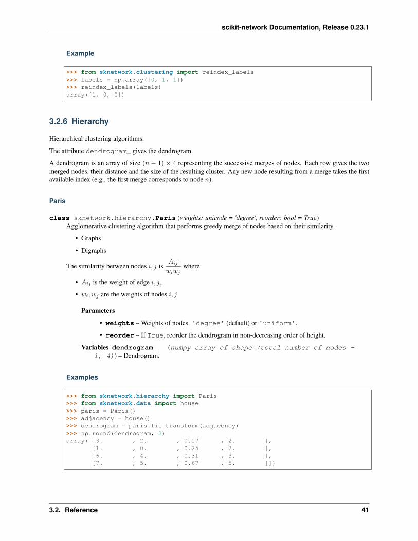
Example
>>> from sknetwork.clustering import reindex_labels>>> labels = np.array([0, 1, 1])>>> reindex_labels(labels)array([1, 0, 0])
3.2.6 Hierarchy
Hierarchical clustering algorithms.
The attribute dendrogram_ gives the dendrogram.
A dendrogram is an array of size (𝑛 − 1) × 4 representing the successive merges of nodes. Each row gives the twomerged nodes, their distance and the size of the resulting cluster. Any new node resulting from a merge takes the firstavailable index (e.g., the first merge corresponds to node 𝑛).
Paris
class sknetwork.hierarchy.Paris(weights: unicode = 'degree', reorder: bool = True)Agglomerative clustering algorithm that performs greedy merge of nodes based on their similarity.
• Graphs
• Digraphs
The similarity between nodes 𝑖, 𝑗 is𝐴𝑖𝑗
𝑤𝑖𝑤𝑗where
• 𝐴𝑖𝑗 is the weight of edge 𝑖, 𝑗,
• 𝑤𝑖, 𝑤𝑗 are the weights of nodes 𝑖, 𝑗
Parameters
• weights – Weights of nodes. 'degree' (default) or 'uniform'.
• reorder – If True, reorder the dendrogram in non-decreasing order of height.
Variables dendrogram_ (numpy array of shape (total number of nodes -1, 4)) – Dendrogram.
Examples
>>> from sknetwork.hierarchy import Paris>>> from sknetwork.data import house>>> paris = Paris()>>> adjacency = house()>>> dendrogram = paris.fit_transform(adjacency)>>> np.round(dendrogram, 2)array([[3. , 2. , 0.17 , 2. ],
[1. , 0. , 0.25 , 2. ],[6. , 4. , 0.31 , 3. ],[7. , 5. , 0.67 , 5. ]])
3.2. Reference 41
scikit-network Documentation, Release 0.23.1
Notes
Each row of the dendrogram = 𝑖, 𝑗, distance, size of cluster 𝑖 + 𝑗.
See also:
scipy.cluster.hierarchy.linkage
References
T. Bonald, B. Charpentier, A. Galland, A. Hollocou (2018). Hierarchical Graph Clustering using Node PairSampling. Workshop on Mining and Learning with Graphs.
fit(adjacency: Union[scipy.sparse.csr.csr_matrix, numpy.ndarray])→ sknetwork.hierarchy.paris.ParisAgglomerative clustering using the nearest neighbor chain.
Parameters adjacency – Adjacency matrix of the graph.
Returns self
Return type Paris
fit_transform(*args, **kwargs)→ numpy.ndarrayFit algorithm to data and return the dendrogram. Same parameters as the fit method.
Returns dendrogram – Dendrogram.
Return type np.ndarray
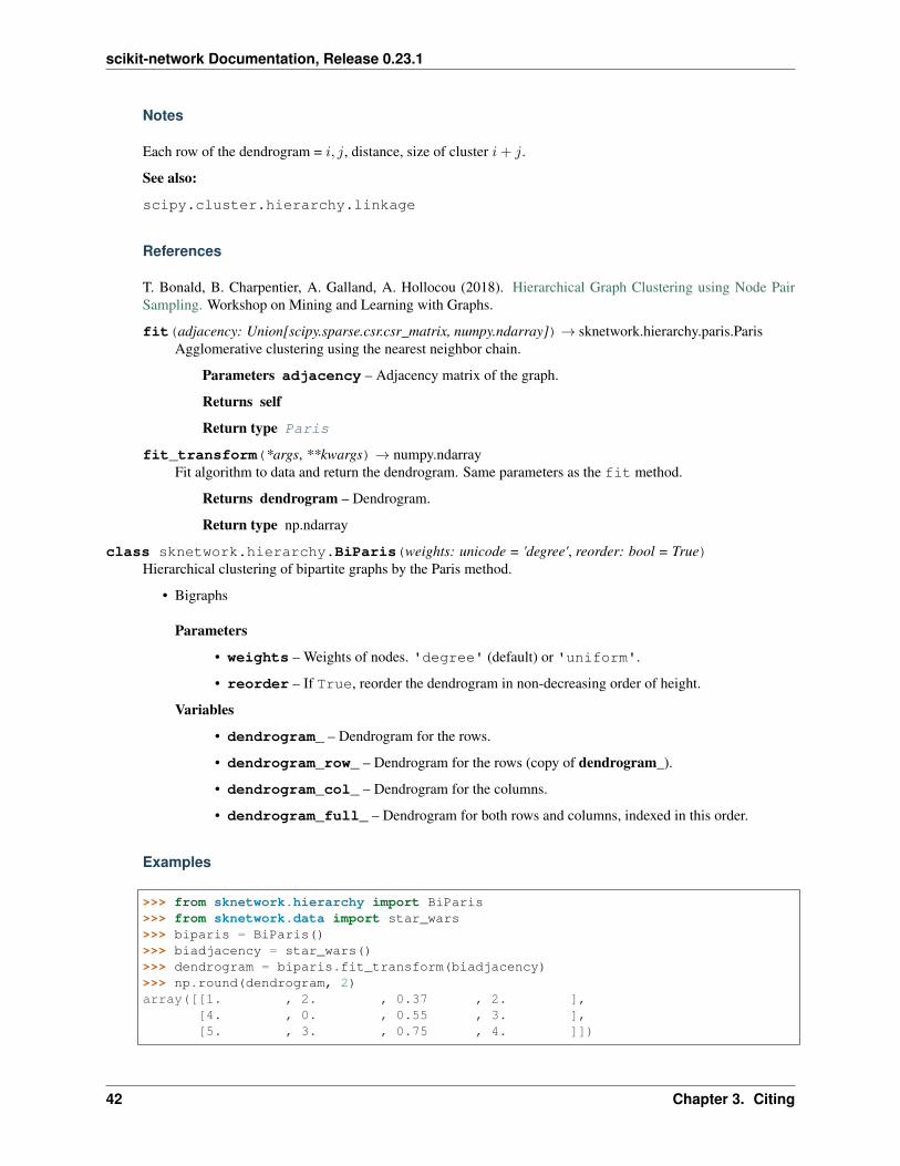
class sknetwork.hierarchy.BiParis(weights: unicode = 'degree', reorder: bool = True)Hierarchical clustering of bipartite graphs by the Paris method.
• Bigraphs
Parameters
• weights – Weights of nodes. 'degree' (default) or 'uniform'.
• reorder – If True, reorder the dendrogram in non-decreasing order of height.
Variables
• dendrogram_ – Dendrogram for the rows.
• dendrogram_row_ – Dendrogram for the rows (copy of dendrogram_).
• dendrogram_col_ – Dendrogram for the columns.
• dendrogram_full_ – Dendrogram for both rows and columns, indexed in this order.
Examples
>>> from sknetwork.hierarchy import BiParis>>> from sknetwork.data import star_wars>>> biparis = BiParis()>>> biadjacency = star_wars()>>> dendrogram = biparis.fit_transform(biadjacency)>>> np.round(dendrogram, 2)array([[1. , 2. , 0.37 , 2. ],
[4. , 0. , 0.55 , 3. ],[5. , 3. , 0.75 , 4. ]])
42 Chapter 3. Citing
scikit-network Documentation, Release 0.23.1
Notes
Each row of the dendrogram = 𝑖, 𝑗, height, size of cluster.
See also:
scipy.cluster.hierarchy.linkage
References
T. Bonald, B. Charpentier, A. Galland, A. Hollocou (2018). Hierarchical Graph Clustering using Node PairSampling. Workshop on Mining and Learning with Graphs.
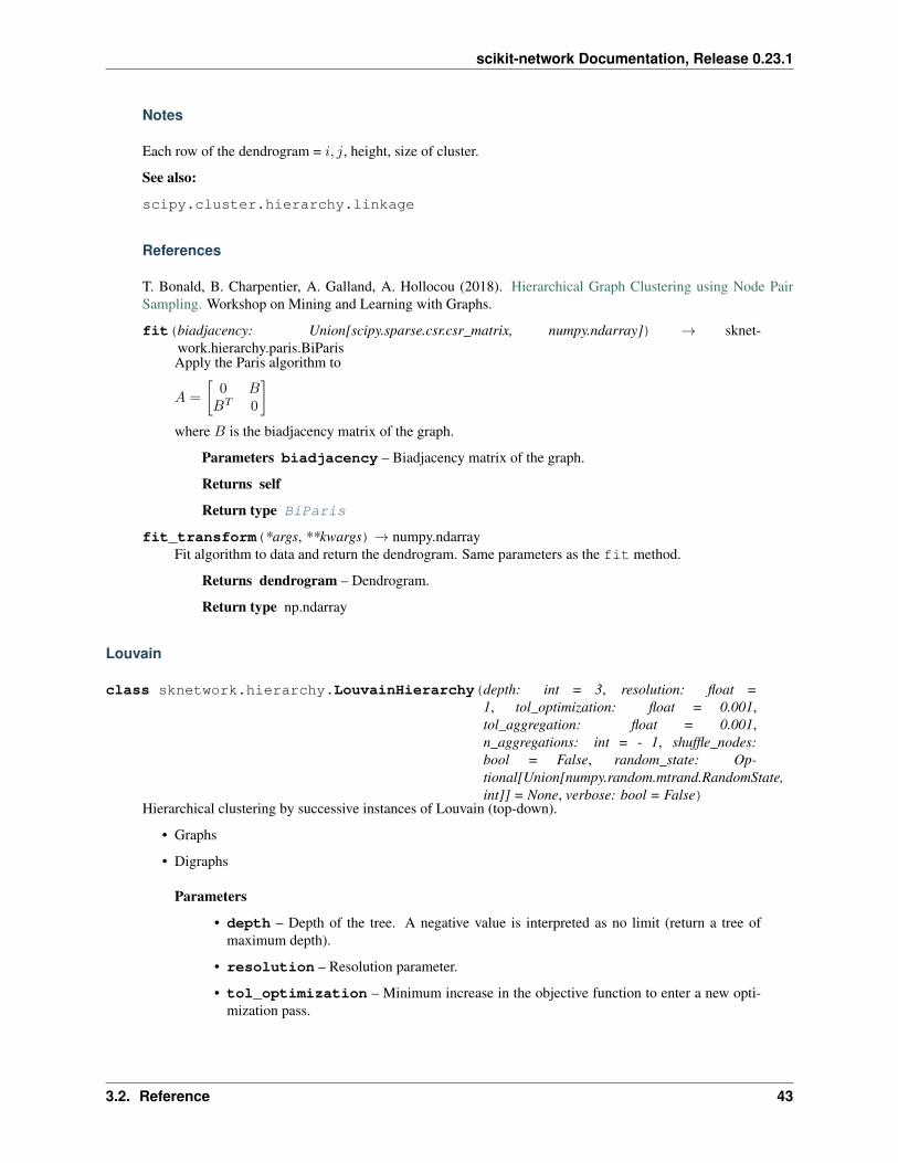
fit(biadjacency: Union[scipy.sparse.csr.csr_matrix, numpy.ndarray]) → sknet-work.hierarchy.paris.BiParisApply the Paris algorithm to
𝐴 =
[0 𝐵𝐵𝑇 0
]where 𝐵 is the biadjacency matrix of the graph.
Parameters biadjacency – Biadjacency matrix of the graph.
Returns self
Return type BiParis
fit_transform(*args, **kwargs)→ numpy.ndarrayFit algorithm to data and return the dendrogram. Same parameters as the fit method.
Returns dendrogram – Dendrogram.
Return type np.ndarray
Louvain
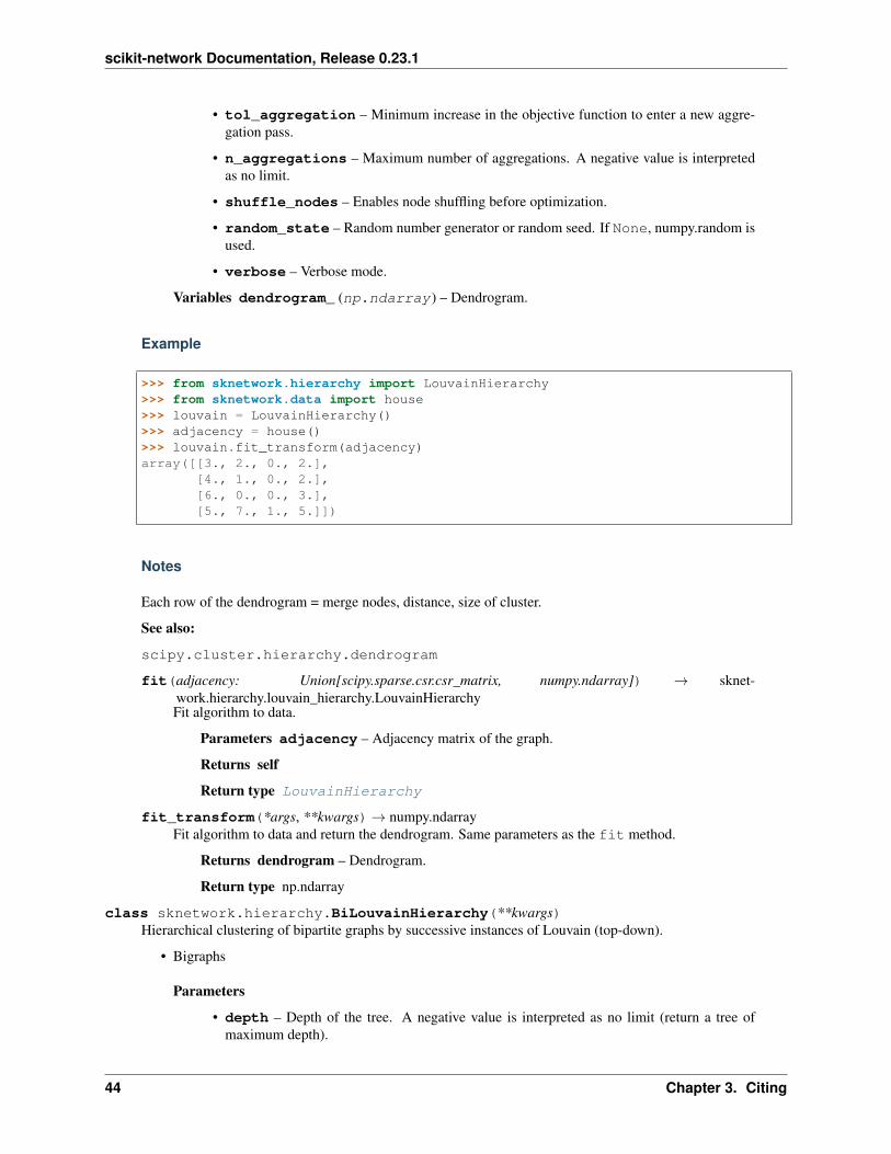
class sknetwork.hierarchy.LouvainHierarchy(depth: int = 3, resolution: float =1, tol_optimization: float = 0.001,tol_aggregation: float = 0.001,n_aggregations: int = - 1, shuffle_nodes:bool = False, random_state: Op-tional[Union[numpy.random.mtrand.RandomState,int]] = None, verbose: bool = False)
Hierarchical clustering by successive instances of Louvain (top-down).
• Graphs
• Digraphs
Parameters
• depth – Depth of the tree. A negative value is interpreted as no limit (return a tree ofmaximum depth).
• resolution – Resolution parameter.
• tol_optimization – Minimum increase in the objective function to enter a new opti-mization pass.
3.2. Reference 43
scikit-network Documentation, Release 0.23.1
• tol_aggregation – Minimum increase in the objective function to enter a new aggre-gation pass.
• n_aggregations – Maximum number of aggregations. A negative value is interpretedas no limit.
• shuffle_nodes – Enables node shuffling before optimization.
• random_state – Random number generator or random seed. If None, numpy.random isused.
• verbose – Verbose mode.
Variables dendrogram_ (np.ndarray) – Dendrogram.
Example
>>> from sknetwork.hierarchy import LouvainHierarchy>>> from sknetwork.data import house>>> louvain = LouvainHierarchy()>>> adjacency = house()>>> louvain.fit_transform(adjacency)array([[3., 2., 0., 2.],
[4., 1., 0., 2.],[6., 0., 0., 3.],[5., 7., 1., 5.]])
Notes
Each row of the dendrogram = merge nodes, distance, size of cluster.
See also:
scipy.cluster.hierarchy.dendrogram
fit(adjacency: Union[scipy.sparse.csr.csr_matrix, numpy.ndarray]) → sknet-work.hierarchy.louvain_hierarchy.LouvainHierarchyFit algorithm to data.
Parameters adjacency – Adjacency matrix of the graph.
Returns self
Return type LouvainHierarchy
fit_transform(*args, **kwargs)→ numpy.ndarrayFit algorithm to data and return the dendrogram. Same parameters as the fit method.
Returns dendrogram – Dendrogram.
Return type np.ndarray
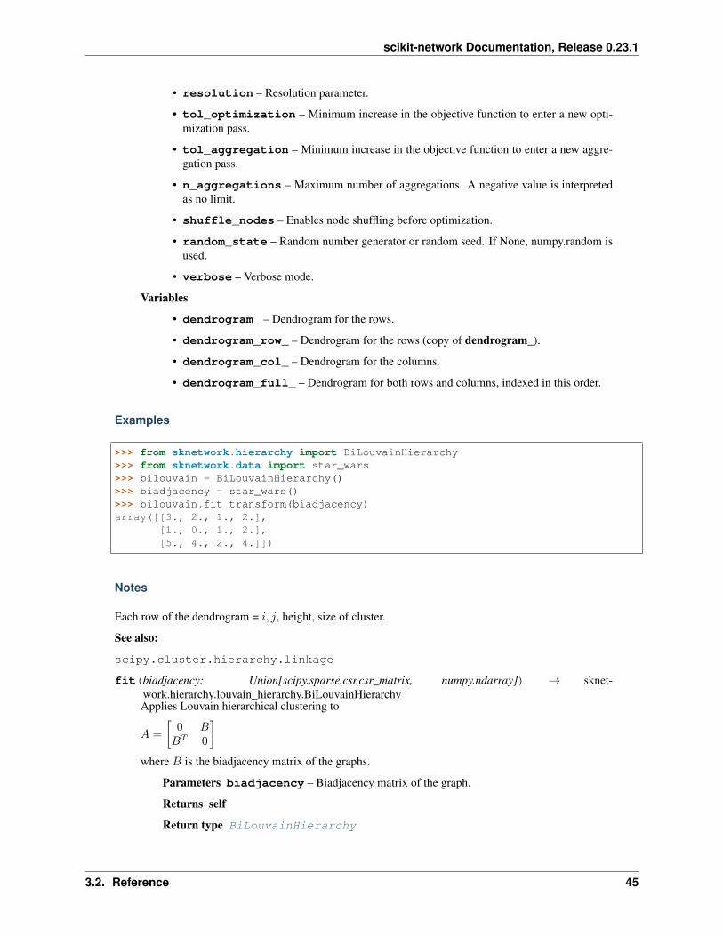
class sknetwork.hierarchy.BiLouvainHierarchy(**kwargs)Hierarchical clustering of bipartite graphs by successive instances of Louvain (top-down).
• Bigraphs
Parameters
• depth – Depth of the tree. A negative value is interpreted as no limit (return a tree ofmaximum depth).
44 Chapter 3. Citing
scikit-network Documentation, Release 0.23.1
• resolution – Resolution parameter.
• tol_optimization – Minimum increase in the objective function to enter a new opti-mization pass.
• tol_aggregation – Minimum increase in the objective function to enter a new aggre-gation pass.
• n_aggregations – Maximum number of aggregations. A negative value is interpretedas no limit.
• shuffle_nodes – Enables node shuffling before optimization.
• random_state – Random number generator or random seed. If None, numpy.random isused.
• verbose – Verbose mode.
Variables
• dendrogram_ – Dendrogram for the rows.
• dendrogram_row_ – Dendrogram for the rows (copy of dendrogram_).
• dendrogram_col_ – Dendrogram for the columns.
• dendrogram_full_ – Dendrogram for both rows and columns, indexed in this order.
Examples
>>> from sknetwork.hierarchy import BiLouvainHierarchy>>> from sknetwork.data import star_wars>>> bilouvain = BiLouvainHierarchy()>>> biadjacency = star_wars()>>> bilouvain.fit_transform(biadjacency)array([[3., 2., 1., 2.],
[1., 0., 1., 2.],[5., 4., 2., 4.]])
Notes
Each row of the dendrogram = 𝑖, 𝑗, height, size of cluster.
See also:
scipy.cluster.hierarchy.linkage
fit(biadjacency: Union[scipy.sparse.csr.csr_matrix, numpy.ndarray]) → sknet-work.hierarchy.louvain_hierarchy.BiLouvainHierarchyApplies Louvain hierarchical clustering to
𝐴 =
[0 𝐵𝐵𝑇 0
]where 𝐵 is the biadjacency matrix of the graphs.
Parameters biadjacency – Biadjacency matrix of the graph.
Returns self
Return type BiLouvainHierarchy
3.2. Reference 45
scikit-network Documentation, Release 0.23.1
fit_transform(*args, **kwargs)→ numpy.ndarrayFit algorithm to data and return the dendrogram. Same parameters as the fit method.
Returns dendrogram – Dendrogram.
Return type np.ndarray
Ward
class sknetwork.hierarchy.Ward(embedding_method: sknetwork.embedding.base.BaseEmbedding= GSVD(n_components=10, regularization=None, rela-tive_regularization=True, factor_row=0.5, factor_col=0.5,factor_singular=0.0, normalized=True, solver='auto'))
Hierarchical clustering by the Ward method.
• Graphs
• Digraphs
Parameters embedding_method – Embedding method (default = GSVD in dimension 10, pro-jected on the unit sphere).
Examples
>>> from sknetwork.hierarchy import Ward>>> from sknetwork.data import karate_club>>> ward = Ward()>>> adjacency = karate_club()>>> dendrogram = ward.fit_transform(adjacency)>>> dendrogram.shape(33, 4)
References
• Ward, J. H., Jr. (1963). Hierarchical grouping to optimize an objective function. Journal of the AmericanStatistical Association.
• Murtagh, F., & Contreras, P. (2012). Algorithms for hierarchical clustering: an overview. Wiley Interdis-ciplinary Reviews: Data Mining and Knowledge Discovery.
fit(adjacency: Union[scipy.sparse.csr.csr_matrix, numpy.ndarray]) → sknet-work.hierarchy.ward.WardApplies embedding method followed by the Ward algorithm.
Parameters adjacency – Adjacency matrix of the graph.
Returns self
Return type Ward
fit_transform(*args, **kwargs)→ numpy.ndarrayFit algorithm to data and return the dendrogram. Same parameters as the fit method.
Returns dendrogram – Dendrogram.
Return type np.ndarray
46 Chapter 3. Citing
scikit-network Documentation, Release 0.23.1
class sknetwork.hierarchy.BiWard(embedding_method: sknet-work.embedding.base.BaseBiEmbedding =GSVD(n_components=10, regularization=None, rela-tive_regularization=True, factor_row=0.5, factor_col=0.5,factor_singular=0.0, normalized=True, solver='auto'),cluster_col: bool = False, cluster_both: bool = False)
Hierarchical clustering of bipartite graphs by the Ward method.
• Bigraphs
Parameters
• embedding_method – Embedding method (default = GSVD in dimension 10, projectedon the unit sphere).
• cluster_col – If True, return a dendrogram for the columns (default = False).
• cluster_both – If True, return a dendrogram for all nodes (co-clustering rows +columns, default = False).
Variables
• dendrogram_ – Dendrogram for the rows.
• dendrogram_row_ – Dendrogram for the rows (copy of dendrogram_).
• dendrogram_col_ – Dendrogram for the columns.
• dendrogram_full_ – Dendrogram for both rows and columns, indexed in this order.
Examples
>>> from sknetwork.hierarchy import BiWard>>> from sknetwork.data import movie_actor>>> biward = BiWard()>>> biadjacency = movie_actor()>>> biward.fit_transform(biadjacency).shape(14, 4)
References
• Ward, J. H., Jr. (1963). Hierarchical grouping to optimize an objective function. Journal of the AmericanStatistical Association, 58, 236–244.
• Murtagh, F., & Contreras, P. (2012). Algorithms for hierarchical clustering: an overview. Wiley Interdis-ciplinary Reviews: Data Mining and Knowledge Discovery, 2(1), 86-97.
fit(biadjacency: Union[scipy.sparse.csr.csr_matrix, numpy.ndarray]) → sknet-work.hierarchy.ward.BiWardApplies the embedding method followed by the Ward algorithm.
Parameters biadjacency – Biadjacency matrix of the graph.
Returns self
Return type BiWard
fit_transform(*args, **kwargs)→ numpy.ndarrayFit algorithm to data and return the dendrogram. Same parameters as the fit method.
3.2. Reference 47
scikit-network Documentation, Release 0.23.1
Returns dendrogram – Dendrogram.
Return type np.ndarray
Metrics
sknetwork.hierarchy.dasgupta_cost(adjacency: scipy.sparse.csr.csr_matrix, dendrogram:numpy.ndarray, weights: str = 'uniform', normalized: bool= False)→ float
Dasgupta’s cost of a hierarchy.
• Graphs
• Digraphs
Expected size (weights = 'uniform') or expected weight (weights = 'degree') of the cluster induced byrandom edge sampling (closest ancestor of the two nodes in the hierarchy).
Parameters
• adjacency – Adjacency matrix of the graph.
• dendrogram – Dendrogram.
• weights – Weights of nodes. 'degree' or 'uniform' (default).
• normalized – If True, normalized cost (between 0 and 1).
Returns cost – Cost.
Return type float
Example
>>> from sknetwork.hierarchy import dasgupta_score, Paris>>> from sknetwork.data import house>>> paris = Paris()>>> adjacency = house()>>> dendrogram = paris.fit_transform(adjacency)>>> cost = dasgupta_cost(adjacency, dendrogram)>>> np.round(cost, 2)3.33
References
Dasgupta, S. (2016). A cost function for similarity-based hierarchical clustering. Proceedings of ACM sympo-sium on Theory of Computing.
sknetwork.hierarchy.dasgupta_score(adjacency: scipy.sparse.csr.csr_matrix, dendrogram:numpy.ndarray, weights: str = 'uniform')→ float
Dasgupta’s score of a hierarchy (quality metric, between 0 and 1).
• Graphs
• Digraphs
Defined as 1 - normalized Dasgupta’s cost.
Parameters
• adjacency – Adjacency matrix of the graph.
48 Chapter 3. Citing
scikit-network Documentation, Release 0.23.1
• dendrogram – Dendrogram.
• weights – Weights of nodes. 'degree' or 'uniform' (default).
Returns score – Score.
Return type float
Example
>>> from sknetwork.hierarchy import dasgupta_score, Paris>>> from sknetwork.data import house>>> paris = Paris()>>> adjacency = house()>>> dendrogram = paris.fit_transform(adjacency)>>> score = dasgupta_score(adjacency, dendrogram)>>> np.round(score, 2)0.33
References
Dasgupta, S. (2016). A cost function for similarity-based hierarchical clustering. Proceedings of ACM sympo-sium on Theory of Computing.
sknetwork.hierarchy.tree_sampling_divergence(adjacency: scipy.sparse.csr.csr_matrix,dendrogram: numpy.ndarray, weights: str= 'degree', normalized: bool = True) →float
Tree sampling divergence of a hierarchy (quality metric).
• Graphs
• Digraphs
Parameters
• adjacency – Adjacency matrix of the graph.
• dendrogram – Dendrogram.
• weights – Weights of nodes. 'degree' (default) or 'uniform'.
• normalized – If True, normalized score (between 0 and 1).
Returns score – Score.
Return type float
Example
>>> from sknetwork.hierarchy import tree_sampling_divergence, Paris>>> from sknetwork.data import house>>> paris = Paris()>>> adjacency = house()>>> dendrogram = paris.fit_transform(adjacency)>>> score = tree_sampling_divergence(adjacency, dendrogram)>>> np.round(score, 2)0.52
3.2. Reference 49
scikit-network Documentation, Release 0.23.1
References
Charpentier, B. & Bonald, T. (2019). Tree Sampling Divergence: An Information-Theoretic Metric for Hierar-chical Graph Clustering. Proceedings of IJCAI.
Cuts
sknetwork.hierarchy.cut_straight(dendrogram: numpy.ndarray, n_clusters: Optional[int] =None, threshold: Optional[float] = None, sort_clusters:bool = True, return_dendrogram: bool = False)→ Union[numpy.ndarray, Tuple[numpy.ndarray,numpy.ndarray]]
Cut a dendrogram and return the corresponding clustering.
Parameters
• dendrogram – Dendrogram.
• n_clusters – Number of clusters (optional). The number of clusters can be larger thann_clusters in case of equal heights in the dendrogram.
• threshold – Threshold on height (optional). If both n_clusters and threshold are None,n_clusters is set to 2.
• sort_clusters – If True, sorts clusters in decreasing order of size.
• return_dendrogram – If True, returns the dendrogram formed by the clusters up tothe root.
Returns
• labels (np.ndarray) – Cluster of each node.
• dendrogram_aggregate (np.ndarray) – Dendrogram starting from clusters (leaves = clus-ters).
Example
>>> from sknetwork.hierarchy import cut_straight>>> dendrogram = np.array([[0, 1, 0, 2], [2, 3, 1, 3]])>>> cut_straight(dendrogram)array([0, 0, 1])
sknetwork.hierarchy.cut_balanced(dendrogram: numpy.ndarray, max_cluster_size: int = 20,sort_clusters: bool = True, return_dendrogram: bool= False) → Union[numpy.ndarray, Tuple[numpy.ndarray,numpy.ndarray]]
Cuts a dendrogram with a constraint on the cluster size and returns the corresponding clustering.
Parameters
• dendrogram – Dendrogram
• max_cluster_size – Maximum size of each cluster.
• sort_clusters – If True, sort labels in decreasing order of cluster size.
• return_dendrogram – If True, returns the dendrogram formed by the clusters up tothe root.
50 Chapter 3. Citing
scikit-network Documentation, Release 0.23.1
Returns
• labels (np.ndarray) – Label of each node.
• dendrogram_aggregate (np.ndarray) – Dendrogram starting from clusters (leaves = clus-ters).
Example
>>> from sknetwork.hierarchy import cut_balanced>>> dendrogram = np.array([[0, 1, 0, 2], [2, 3, 1, 3]])>>> cut_balanced(dendrogram, 2)array([0, 0, 1])
3.2.7 Ranking
Node ranking algorithms.
The attribute scores_ assigns a score of importance to each node of the graph.
PageRank
class sknetwork.ranking.PageRank(damping_factor: float = 0.85, solver: str = 'piteration',n_iter: int = 10, tol: float = 1e-06)
PageRank of each node, corresponding to its frequency of visit by a random walk.
The random walk restarts with some fixed probability. The restart distribution can be personalized by the user.This variant is known as Personalized PageRank.
• Graphs
• Digraphs
Parameters
• damping_factor (float) – Probability to continue the random walk.
• solver (str) –
– 'piteration', use power iteration for a given number of iterations.
– 'diteration', use asynchronous parallel diffusion for a given number of iterations.
– 'lanczos', use eigensolver with a given tolerance.
– 'bicgstab', use Biconjugate Gradient Stabilized method for a given tolerance.
– 'RH', use a Ruffini-Horner polynomial evaluation.
– 'push', use push-based algorithm for a given tolerance
• n_iter (int) – Number of iterations for some solvers.
• tol (float) – Tolerance for the convergence of some solvers.
Variables scores_ (np.ndarray) – PageRank score of each node.
3.2. Reference 51
scikit-network Documentation, Release 0.23.1
Example
>>> from sknetwork.ranking import PageRank>>> from sknetwork.data import house>>> pagerank = PageRank()>>> adjacency = house()>>> seeds = {0: 1}>>> scores = pagerank.fit_transform(adjacency, seeds)>>> np.round(scores, 2)array([0.29, 0.24, 0.12, 0.12, 0.24])
References
Page, L., Brin, S., Motwani, R., & Winograd, T. (1999). The PageRank citation ranking: Bringing order to theweb. Stanford InfoLab.
fit(adjacency: Union[scipy.sparse.csr.csr_matrix, numpy.ndarray,scipy.sparse.linalg.interface.LinearOperator], seeds: Optional[Union[numpy.ndarray, dict]]= None)→ sknetwork.ranking.pagerank.PageRankFit algorithm to data.
Parameters
• adjacency – Adjacency matrix.
• seeds – Parameter to be used for Personalized PageRank. Restart distribution as a vectoror a dict (node: weight). If None, the uniform distribution is used (no personalization,default).
Returns self
Return type PageRank
fit_transform(*args, **kwargs)→ numpy.ndarrayFit algorithm to data and return the scores. Same parameters as the fit method.
Returns scores – Scores.
Return type np.ndarray
class sknetwork.ranking.BiPageRank(damping_factor: float = 0.85, solver: str = 'piteration',n_iter: int = 10, tol: float = 0)
Compute the PageRank of each node through a random walk in the bipartite graph.
• Bigraphs
Parameters
• damping_factor (float) – Probability to continue the random walk.
• solver (str) –
– piteration, use power iteration for a given number of iterations.
– diteration, use asynchronous parallel diffusion for a given number of iterations.
– lanczos, use eigensolver for a given tolerance.
– bicgstab, use Biconjugate Gradient Stabilized method for a given tolerance.
• n_iter (int) – Number of iterations for some solvers.
• tol (float) – Tolerance for the convergence of some solvers.
52 Chapter 3. Citing
scikit-network Documentation, Release 0.23.1
Variables
• scores_ (np.ndarray) – PageRank score of each row.
• scores_row_ (np.ndarray) – PageRank score of each row (copy of scores_).
• scores_col_ (np.ndarray) – PageRank score of each column.
Example
>>> from sknetwork.ranking import BiPageRank>>> from sknetwork.data import star_wars>>> bipagerank = BiPageRank()>>> biadjacency = star_wars()>>> seeds = {0: 1}>>> scores = bipagerank.fit_transform(biadjacency, seeds)>>> np.round(scores, 2)array([0.45, 0.11, 0.28, 0.17])
fit(biadjacency: Union[scipy.sparse.csr.csr_matrix, numpy.ndarray], seeds_row: Op-tional[Union[numpy.ndarray, dict]] = None, seeds_col: Optional[Union[numpy.ndarray, dict]] =None)→ sknetwork.ranking.pagerank.BiPageRankFit algorithm to data.
Parameters
• biadjacency – Biadjacency matrix.
• seeds_row – Parameter to be used for Personalized BiPageRank. Restart distributionas vectors or dicts on rows, columns (node: weight). If both seeds_row and seeds_col areNone (default), the uniform distribution on rows is used.
• seeds_col – Parameter to be used for Personalized BiPageRank. Restart distributionas vectors or dicts on rows, columns (node: weight). If both seeds_row and seeds_col areNone (default), the uniform distribution on rows is used.
Returns self
Return type BiPageRank
fit_transform(*args, **kwargs)→ numpy.ndarrayFit algorithm to data and return the scores. Same parameters as the fit method.
Returns scores – Scores.
Return type np.ndarray
Diffusion
class sknetwork.ranking.Diffusion(n_iter: int = 3, damping_factor: Optional[float] = None)Ranking by diffusion along the edges (heat equation).
• Graphs
• Digraphs
Parameters
• n_iter (int) – Number of steps of the diffusion in discrete time (must be positive).
• damping_factor (float (optional)) – Damping factor (default value = 1).
3.2. Reference 53
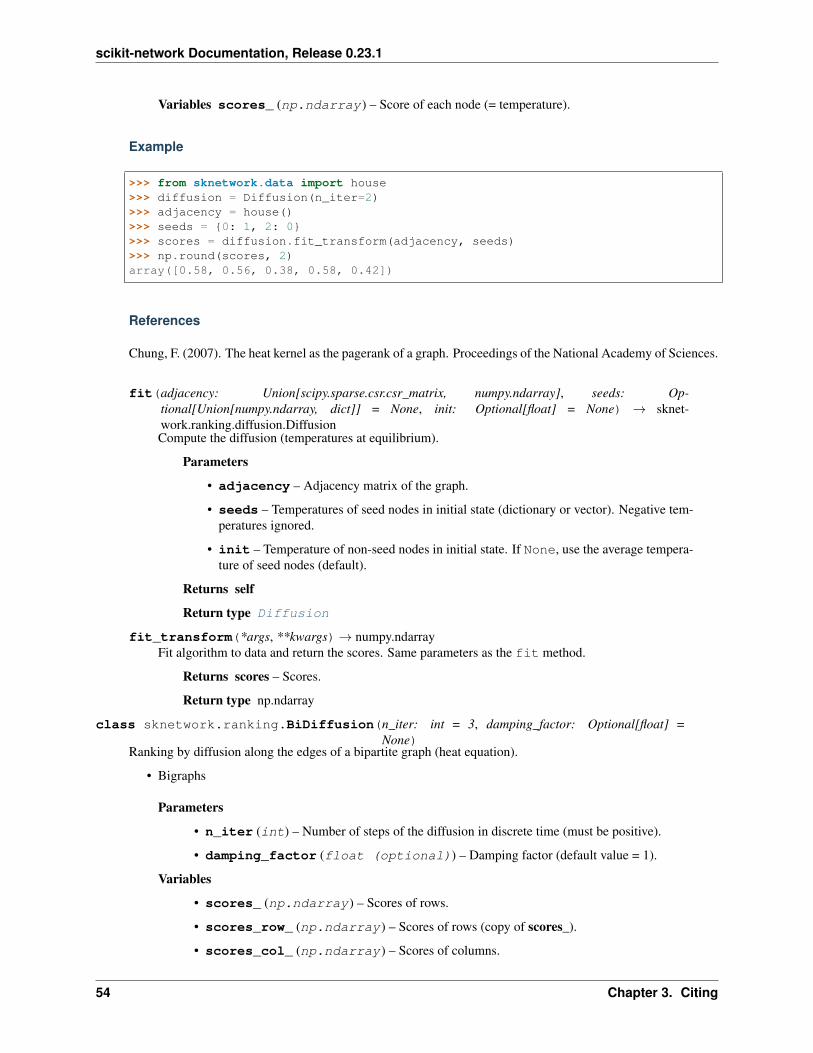
scikit-network Documentation, Release 0.23.1
Variables scores_ (np.ndarray) – Score of each node (= temperature).
Example
>>> from sknetwork.data import house>>> diffusion = Diffusion(n_iter=2)>>> adjacency = house()>>> seeds = {0: 1, 2: 0}>>> scores = diffusion.fit_transform(adjacency, seeds)>>> np.round(scores, 2)array([0.58, 0.56, 0.38, 0.58, 0.42])
References
Chung, F. (2007). The heat kernel as the pagerank of a graph. Proceedings of the National Academy of Sciences.
fit(adjacency: Union[scipy.sparse.csr.csr_matrix, numpy.ndarray], seeds: Op-tional[Union[numpy.ndarray, dict]] = None, init: Optional[float] = None) → sknet-work.ranking.diffusion.DiffusionCompute the diffusion (temperatures at equilibrium).
Parameters
• adjacency – Adjacency matrix of the graph.
• seeds – Temperatures of seed nodes in initial state (dictionary or vector). Negative tem-peratures ignored.
• init – Temperature of non-seed nodes in initial state. If None, use the average tempera-ture of seed nodes (default).
Returns self
Return type Diffusion
fit_transform(*args, **kwargs)→ numpy.ndarrayFit algorithm to data and return the scores. Same parameters as the fit method.
Returns scores – Scores.
Return type np.ndarray
class sknetwork.ranking.BiDiffusion(n_iter: int = 3, damping_factor: Optional[float] =None)
Ranking by diffusion along the edges of a bipartite graph (heat equation).
• Bigraphs
Parameters
• n_iter (int) – Number of steps of the diffusion in discrete time (must be positive).
• damping_factor (float (optional)) – Damping factor (default value = 1).
Variables
• scores_ (np.ndarray) – Scores of rows.
• scores_row_ (np.ndarray) – Scores of rows (copy of scores_).
• scores_col_ (np.ndarray) – Scores of columns.
54 Chapter 3. Citing
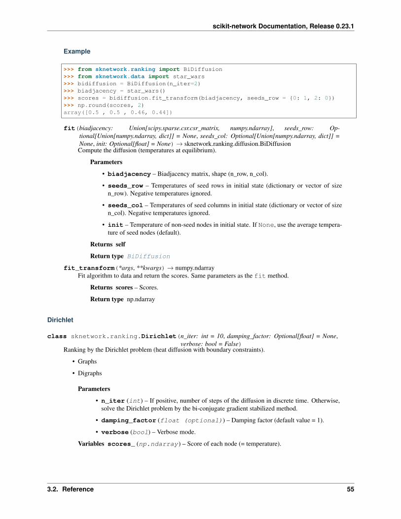
scikit-network Documentation, Release 0.23.1
Example
>>> from sknetwork.ranking import BiDiffusion>>> from sknetwork.data import star_wars>>> bidiffusion = BiDiffusion(n_iter=2)>>> biadjacency = star_wars()>>> scores = bidiffusion.fit_transform(biadjacency, seeds_row = {0: 1, 2: 0})>>> np.round(scores, 2)array([0.5 , 0.5 , 0.46, 0.44])
fit(biadjacency: Union[scipy.sparse.csr.csr_matrix, numpy.ndarray], seeds_row: Op-tional[Union[numpy.ndarray, dict]] = None, seeds_col: Optional[Union[numpy.ndarray, dict]] =None, init: Optional[float] = None)→ sknetwork.ranking.diffusion.BiDiffusionCompute the diffusion (temperatures at equilibrium).
Parameters
• biadjacency – Biadjacency matrix, shape (n_row, n_col).
• seeds_row – Temperatures of seed rows in initial state (dictionary or vector of sizen_row). Negative temperatures ignored.
• seeds_col – Temperatures of seed columns in initial state (dictionary or vector of sizen_col). Negative temperatures ignored.
• init – Temperature of non-seed nodes in initial state. If None, use the average tempera-ture of seed nodes (default).
Returns self
Return type BiDiffusion
fit_transform(*args, **kwargs)→ numpy.ndarrayFit algorithm to data and return the scores. Same parameters as the fit method.
Returns scores – Scores.
Return type np.ndarray
Dirichlet
class sknetwork.ranking.Dirichlet(n_iter: int = 10, damping_factor: Optional[float] = None,verbose: bool = False)
Ranking by the Dirichlet problem (heat diffusion with boundary constraints).
• Graphs
• Digraphs
Parameters
• n_iter (int) – If positive, number of steps of the diffusion in discrete time. Otherwise,solve the Dirichlet problem by the bi-conjugate gradient stabilized method.
• damping_factor (float (optional)) – Damping factor (default value = 1).
• verbose (bool) – Verbose mode.
Variables scores_ (np.ndarray) – Score of each node (= temperature).
3.2. Reference 55
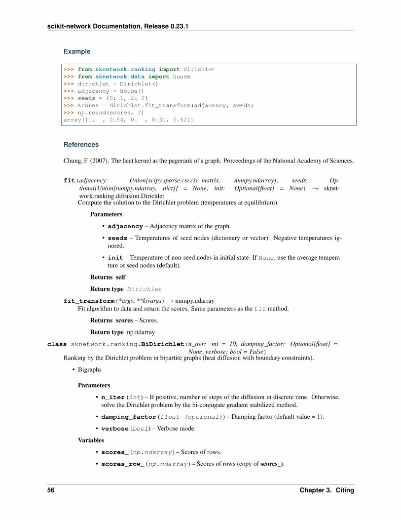
scikit-network Documentation, Release 0.23.1
Example
>>> from sknetwork.ranking import Dirichlet>>> from sknetwork.data import house>>> dirichlet = Dirichlet()>>> adjacency = house()>>> seeds = {0: 1, 2: 0}>>> scores = dirichlet.fit_transform(adjacency, seeds)>>> np.round(scores, 2)array([1. , 0.54, 0. , 0.31, 0.62])
References
Chung, F. (2007). The heat kernel as the pagerank of a graph. Proceedings of the National Academy of Sciences.
fit(adjacency: Union[scipy.sparse.csr.csr_matrix, numpy.ndarray], seeds: Op-tional[Union[numpy.ndarray, dict]] = None, init: Optional[float] = None) → sknet-work.ranking.diffusion.DirichletCompute the solution to the Dirichlet problem (temperatures at equilibrium).
Parameters
• adjacency – Adjacency matrix of the graph.
• seeds – Temperatures of seed nodes (dictionary or vector). Negative temperatures ig-nored.
• init – Temperature of non-seed nodes in initial state. If None, use the average tempera-ture of seed nodes (default).
Returns self
Return type Dirichlet
fit_transform(*args, **kwargs)→ numpy.ndarrayFit algorithm to data and return the scores. Same parameters as the fit method.
Returns scores – Scores.
Return type np.ndarray
class sknetwork.ranking.BiDirichlet(n_iter: int = 10, damping_factor: Optional[float] =None, verbose: bool = False)
Ranking by the Dirichlet problem in bipartite graphs (heat diffusion with boundary constraints).
• Bigraphs
Parameters
• n_iter (int) – If positive, number of steps of the diffusion in discrete time. Otherwise,solve the Dirichlet problem by the bi-conjugate gradient stabilized method.
• damping_factor (float (optional)) – Damping factor (default value = 1).
• verbose (bool) – Verbose mode.
Variables
• scores_ (np.ndarray) – Scores of rows.
• scores_row_ (np.ndarray) – Scores of rows (copy of scores_).
56 Chapter 3. Citing
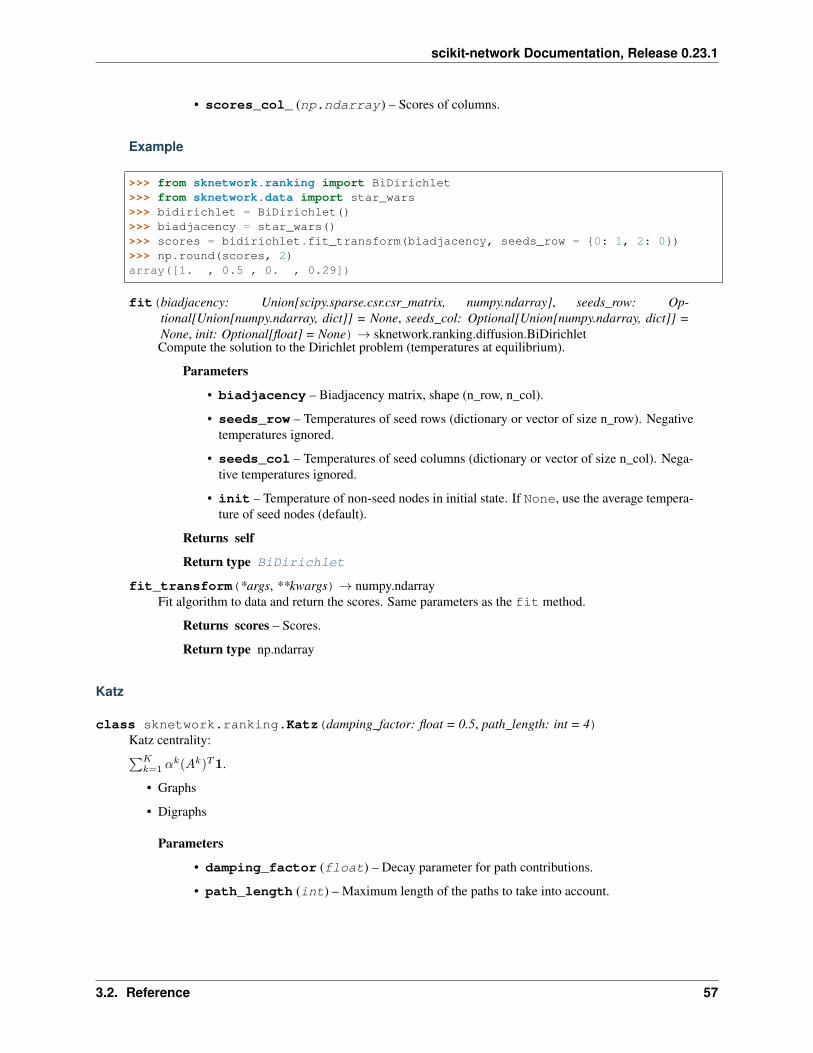
scikit-network Documentation, Release 0.23.1
• scores_col_ (np.ndarray) – Scores of columns.
Example
>>> from sknetwork.ranking import BiDirichlet>>> from sknetwork.data import star_wars>>> bidirichlet = BiDirichlet()>>> biadjacency = star_wars()>>> scores = bidirichlet.fit_transform(biadjacency, seeds_row = {0: 1, 2: 0})>>> np.round(scores, 2)array([1. , 0.5 , 0. , 0.29])
fit(biadjacency: Union[scipy.sparse.csr.csr_matrix, numpy.ndarray], seeds_row: Op-tional[Union[numpy.ndarray, dict]] = None, seeds_col: Optional[Union[numpy.ndarray, dict]] =None, init: Optional[float] = None)→ sknetwork.ranking.diffusion.BiDirichletCompute the solution to the Dirichlet problem (temperatures at equilibrium).
Parameters
• biadjacency – Biadjacency matrix, shape (n_row, n_col).
• seeds_row – Temperatures of seed rows (dictionary or vector of size n_row). Negativetemperatures ignored.
• seeds_col – Temperatures of seed columns (dictionary or vector of size n_col). Nega-tive temperatures ignored.
• init – Temperature of non-seed nodes in initial state. If None, use the average tempera-ture of seed nodes (default).
Returns self
Return type BiDirichlet
fit_transform(*args, **kwargs)→ numpy.ndarrayFit algorithm to data and return the scores. Same parameters as the fit method.
Returns scores – Scores.
Return type np.ndarray
Katz
class sknetwork.ranking.Katz(damping_factor: float = 0.5, path_length: int = 4)Katz centrality:∑𝐾
𝑘=1 𝛼𝑘(𝐴𝑘)𝑇1.
• Graphs
• Digraphs
Parameters
• damping_factor (float) – Decay parameter for path contributions.
• path_length (int) – Maximum length of the paths to take into account.
3.2. Reference 57
scikit-network Documentation, Release 0.23.1
Examples
>>> from sknetwork.data.toy_graphs import house>>> adjacency = house()>>> katz = Katz()>>> scores = katz.fit_transform(adjacency)>>> np.round(scores, 2)array([6.5 , 8.25, 5.62, 5.62, 8.25])
References
Katz, L. (1953). A new status index derived from sociometric analysis. Psychometrika, 18(1), 39-43.
fit(adjacency: Union[scipy.sparse.csr.csr_matrix, numpy.ndarray,scipy.sparse.linalg.interface.LinearOperator])→ sknetwork.ranking.katz.KatzKatz centrality.
Parameters adjacency – Adjacency matrix of the graph.
Returns self
Return type Katz
fit_transform(*args, **kwargs)→ numpy.ndarrayFit algorithm to data and return the scores. Same parameters as the fit method.
Returns scores – Scores.
Return type np.ndarray
class sknetwork.ranking.BiKatz(damping_factor: float = 0.5, path_length: int = 4)Katz centrality for bipartite graphs.
• Bigraphs
Parameters
• damping_factor (float) – Decay parameter for path contributions.
• path_length (int) – Maximum length of the paths to take into account.
Examples
>>> from sknetwork.data.toy_graphs import star_wars>>> biadjacency = star_wars()>>> bikatz = BiKatz()>>> scores = bikatz.fit_transform(biadjacency)>>> np.round(scores, 2)array([6.38, 3.06, 8.81, 5.75])
58 Chapter 3. Citing
scikit-network Documentation, Release 0.23.1
References
Katz, L. (1953). A new status index derived from sociometric analysis. Psychometrika, 18(1), 39-43.
fit(biadjacency: Union[scipy.sparse.csr.csr_matrix, numpy.ndarray]) → sknet-work.ranking.katz.BiKatzKatz centrality.
Parameters biadjacency – Biadjacency matrix of the graph.
Returns self
Return type BiKatz
fit_transform(*args, **kwargs)→ numpy.ndarrayFit algorithm to data and return the scores. Same parameters as the fit method.
Returns scores – Scores.
Return type np.ndarray
HITS
class sknetwork.ranking.HITS(solver: Union[str, sknetwork.linalg.svd_solver.SVDSolver] = 'auto',**kwargs)
Hub and authority scores of each node. For bipartite graphs, the hub score is computed on rows and the authorityscore on columns.
• Graphs
• Digraphs
• Bigraphs
Parameters
• solver ('auto', 'halko', 'lanczos' or SVDSolver) – Which singular valuesolver to use.
– 'auto' call the auto_solver function.
– 'halko': randomized method, fast but less accurate than 'lanczos' for ill-conditioned matrices.
– 'lanczos': power-iteration based method.
– SVDSolver: custom solver.
• **kwargs – See sknetwork.linalg.svd_solver.LanczosSVD or sknet-work.linalg.svd_solver.HalkoSVD.
Variables
• scores_ (np.ndarray) – Hub score of each row.
• scores_row_ (np.ndarray) – Hub score of each row (copy of scores_row_).
• scores_col_ (np.ndarray) – Authority score of each column.
3.2. Reference 59
scikit-network Documentation, Release 0.23.1
Example
>>> from sknetwork.ranking import HITS>>> from sknetwork.data import star_wars>>> hits = HITS()>>> biadjacency = star_wars()>>> scores = hits.fit_transform(biadjacency)>>> np.round(scores, 2)array([0.5 , 0.23, 0.69, 0.46])
References
Kleinberg, J. M. (1999). Authoritative sources in a hyperlinked environment. Journal of the ACM (JACM),46(5), 604-632.
fit(adjacency: Union[scipy.sparse.csr.csr_matrix, numpy.ndarray])→ sknetwork.ranking.hits.HITSCompute HITS algorithm with a spectral method.
Parameters adjacency – Adjacency or biadjacency matrix of the graph.
Returns self
Return type HITS
fit_transform(*args, **kwargs)→ numpy.ndarrayFit algorithm to data and return the scores. Same parameters as the fit method.
Returns scores – Scores.
Return type np.ndarray
Betweenness centrality
class sknetwork.ranking.Betweenness(normalized: bool = False)Betweenness centrality, based on Brandes’ algorithm.
• Graphs
Variables scores_ (np.ndarray) – Betweenness centrality value of each node
Example
>>> from sknetwork.ranking import Betweenness>>> from sknetwork.data.toy_graphs import bow_tie>>> betweenness = Betweenness()>>> adjacency = bow_tie()>>> scores = betweenness.fit_transform(adjacency)>>> scoresarray([4., 0., 0., 0., 0.])
60 Chapter 3. Citing
scikit-network Documentation, Release 0.23.1
References
Brandes, Ulrik (2001). A faster algorithm for betweenness centrality. Journal of Mathematical Sociology.
fit_transform(*args, **kwargs)→ numpy.ndarrayFit algorithm to data and return the scores. Same parameters as the fit method.
Returns scores – Scores.
Return type np.ndarray
Closeness centrality
class sknetwork.ranking.Closeness(method: str = 'exact', tol: float = 0.1, n_jobs: Optional[int]= None)
Closeness centrality of each node in a connected graph, corresponding to the average length of the shortest pathsfrom that node to all the other ones.
For a directed graph, the closeness centrality is computed in terms of outgoing paths.
• Graphs
• Digraphs
Parameters
• method – Denotes if the results should be exact or approximate.
• tol (float) – If method=='approximate', the allowed tolerance on each score en-try.
• n_jobs – If an integer value is given, denotes the number of workers to use (-1 means themaximum number will be used). If None, no parallel computations are made.
Variables scores_ (np.ndarray) – Closeness centrality of each node.
Example
>>> from sknetwork.ranking import Closeness>>> from sknetwork.data import cyclic_digraph>>> closeness = Closeness()>>> adjacency = cyclic_digraph(3)>>> scores = closeness.fit_transform(adjacency)>>> np.round(scores, 2)array([0.67, 0.67, 0.67])
References
Eppstein, D., & Wang, J. (2001, January). Fast approximation of centrality. In Proceedings of the twelfth annualACM-SIAM symposium on Discrete algorithms (pp. 228-229). Society for Industrial and Applied Mathematics.
fit(adjacency: Union[scipy.sparse.csr.csr_matrix, numpy.ndarray]) → sknet-work.ranking.closeness.ClosenessCloseness centrality for connected graphs.
Parameters adjacency – Adjacency matrix of the graph.
Returns self
3.2. Reference 61
scikit-network Documentation, Release 0.23.1
Return type Closeness
fit_transform(*args, **kwargs)→ numpy.ndarrayFit algorithm to data and return the scores. Same parameters as the fit method.
Returns scores – Scores.
Return type np.ndarray
Harmonic centrality
class sknetwork.ranking.Harmonic(n_jobs: Optional[int] = None)Harmonic centrality of each node in a connected graph, corresponding to the average inverse length of theshortest paths from that node to all the other ones.
For a directed graph, the harmonic centrality is computed in terms of outgoing paths.
• Graphs
• Digraphs
Parameters n_jobs – If an integer value is given, denotes the number of workers to use (-1 meansthe maximum number will be used). If None, no parallel computations are made.
Variables scores_ (np.ndarray) – Harmonic centrality of each node.
Example
>>> from sknetwork.ranking import Harmonic>>> from sknetwork.data import house>>> harmonic = Harmonic()>>> adjacency = house()>>> scores = harmonic.fit_transform(adjacency)>>> np.round(scores, 2)array([3. , 3.5, 3. , 3. , 3.5])
References
Marchiori, M., & Latora, V. (2000). Harmony in the small-world. Physica A: Statistical Mechanics and itsApplications, 285(3-4), 539-546.
fit(adjacency: Union[scipy.sparse.csr.csr_matrix, numpy.ndarray]) → sknet-work.ranking.harmonic.HarmonicHarmonic centrality for connected graphs.
Parameters adjacency – Adjacency matrix of the graph.
Returns self
Return type Harmonic
fit_transform(*args, **kwargs)→ numpy.ndarrayFit algorithm to data and return the scores. Same parameters as the fit method.
Returns scores – Scores.
Return type np.ndarray
62 Chapter 3. Citing
scikit-network Documentation, Release 0.23.1
Post-processing
sknetwork.ranking.top_k(scores: numpy.ndarray, k: int = 1)Index of the k elements with highest value.
Parameters
• scores (np.ndarray) – Array of values.
• k (int) – Number of elements to return.
Examples
>>> scores = np.array([0, 1, 0, 0.5])>>> top_k(scores, k=2)array([1, 3])
Notes
This is a basic implementation that sorts the entire array to find its top k elements.
3.2.8 Classification
Node classification algorithms.
The attribute labels_ assigns a label to each node of the graph.
PageRank
class sknetwork.classification.PageRankClassifier(damping_factor: float = 0.85,solver: str = 'piteration', n_iter: int= 10, tol: float = 0.0, n_jobs: Op-tional[int] = None, verbose: bool =False)
Node classification by multiple personalized PageRanks.
• Graphs
• Digraphs
Parameters
• damping_factor – Probability to continue the random walk.
• solver (str) – Which solver to use: ‘piteration’, ‘diteration’, ‘bicgstab’, ‘lanczos’.
• n_iter (int) – Number of iterations for some of the solvers such as 'piteration' or'diteration'.
• tol (float) – Tolerance for the convergence of some solvers such as 'bicgstab' or'lanczos'.
Variables
• labels_ (np.ndarray) – Label of each node (hard classification).
3.2. Reference 63
scikit-network Documentation, Release 0.23.1
• membership_ (sparse.csr_matrix) – Membership matrix (soft classification,columns = labels).
Example
>>> from sknetwork.classification import PageRankClassifier>>> from sknetwork.data import karate_club>>> pagerank = PageRankClassifier()>>> graph = karate_club(metadata=True)>>> adjacency = graph.adjacency>>> labels_true = graph.labels>>> seeds = {0: labels_true[0], 33: labels_true[33]}>>> labels_pred = pagerank.fit_transform(adjacency, seeds)>>> np.round(np.mean(labels_pred == labels_true), 2)0.97
References
Lin, F., & Cohen, W. W. (2010). Semi-supervised classification of network data using very few labels. In IEEEInternational Conference on Advances in Social Networks Analysis and Mining.
fit(adjacency: Union[scipy.sparse.csr.csr_matrix, numpy.ndarray], seeds: Union[numpy.ndarray,dict])→ sknetwork.classification.base_rank.RankClassifierFit algorithm to the data.
Parameters
• adjacency – Adjacency matrix of the graph.
• seeds – Seed nodes (labels as dictionary or array; negative values ignored).
Returns self
Return type RankClassifier
fit_transform(*args, **kwargs)→ numpy.ndarrayFit algorithm to the data and return the labels. Same parameters as the fit method.
Returns labels – Labels.
Return type np.ndarray
score(label: int)Classification scores for a given label.
Parameters label (int) – The label index of the class.
Returns scores – Classification scores of shape (number of nodes,).
Return type np.ndarray
class sknetwork.classification.BiPageRankClassifier(damping_factor: float = 0.85,solver: str = 'piteration', n_iter:int = 10, tol: float = 0.0, n_jobs:Optional[int] = None, verbose:bool = False)
Node classification for bipartite graphs by multiple personalized PageRanks .
• Bigraphs
Parameters
64 Chapter 3. Citing
scikit-network Documentation, Release 0.23.1
• damping_factor – Probability to continue the random walk.
• solver (str) – Which solver to use: ‘piteration’, ‘diteration’, ‘bicgstab’, ‘lanczos’.
• n_iter (int) – Number of iterations for some of the solvers such as 'piteration' or'diteration'.
• tol (float) – Tolerance for the convergence of some solvers such as 'bicgstab' or'lanczos'.
Variables
• labels_ (np.ndarray) – Label of each row.
• labels_row_ (np.ndarray) – Label of each row (copy of labels_).
• labels_col_ (np.ndarray) – Label of each column.
• membership_ (sparse.csr_matrix) – Membership matrix of rows (soft classifica-tion, labels on columns).
• membership_row_ (sparse.csr_matrix) – Membership matrix of rows (copy ofmembership_).
• membership_col_ (sparse.csr_matrix) – Membership matrix of columns.
Example
>>> from sknetwork.classification import BiPageRankClassifier>>> from sknetwork.data import star_wars>>> bipagerank = BiPageRankClassifier()>>> biadjacency = star_wars()>>> seeds = {0: 1, 2: 0}>>> bipagerank.fit_transform(biadjacency, seeds)array([1, 1, 0, 0])
fit(biadjacency: Union[scipy.sparse.csr.csr_matrix, numpy.ndarray], seeds_row:Union[numpy.ndarray, dict], seeds_col: Optional[Union[numpy.ndarray, dict]] = None) →sknetwork.classification.base_rank.RankClassifierCompute labels.
Parameters
• biadjacency – Biadjacency matrix of the graph.
• seeds_row – Seed rows (labels as dictionary or array; negative values ignored).
• seeds_col – Seed columns (optional). Same format.
Returns self
Return type BiPageRankClassifier
fit_transform(*args, **kwargs)→ numpy.ndarrayFit algorithm to the data and return the labels. Same parameters as the fit method.
Returns labels – Labels.
Return type np.ndarray
score(label: int)Classification scores for a given label.
Parameters label (int) – The label index of the class.
3.2. Reference 65
scikit-network Documentation, Release 0.23.1
Returns scores – Classification scores of shape (number of nodes,).
Return type np.ndarray
Diffusion
class sknetwork.classification.DiffusionClassifier(n_iter: int = 10, damping_factor:Optional[float] = None, n_jobs:Optional[int] = None)
Node classification using multiple diffusions.
• Graphs
• Digraphs
Parameters
• n_iter (int) – Number of steps of the diffusion in discrete time (must be positive).
• damping_factor (float (optional)) – Damping factor (default value = 1).
• n_jobs – If positive, number of parallel jobs allowed (-1 means maximum number). IfNone, no parallel computations are made.
Variables
• labels_ (np.ndarray) – Label of each node (hard classification).
• membership_ (sparse.csr_matrix) – Membership matrix (soft classification, la-bels on columns).
Example
>>> from sknetwork.data import karate_club>>> diffusion = DiffusionClassifier()>>> graph = karate_club(metadata=True)>>> adjacency = graph.adjacency>>> labels_true = graph.labels>>> seeds = {0: labels_true[0], 33: labels_true[33]}>>> labels_pred = diffusion.fit_transform(adjacency, seeds)>>> np.round(np.mean(labels_pred == labels_true), 2)0.94
References
• de Lara, N., & Bonald, T. (2020). A Consistent Diffusion-Based Algorithm for Semi-Supervised Classifi-cation on Graphs. arXiv preprint arXiv:2008.11944.
• Zhu, X., Lafferty, J., & Rosenfeld, R. (2005). Semi-supervised learning with graphs (Doctoral dissertation,Carnegie Mellon University, language technologies institute, school of computer science).
fit(adjacency: Union[scipy.sparse.csr.csr_matrix, numpy.ndarray], seeds: Union[numpy.ndarray,dict])→ sknetwork.classification.base_rank.RankClassifierFit algorithm to the data.
Parameters
• adjacency – Adjacency matrix of the graph.
66 Chapter 3. Citing
scikit-network Documentation, Release 0.23.1
• seeds – Seed nodes (labels as dictionary or array; negative values ignored).
Returns self
Return type RankClassifier
fit_transform(*args, **kwargs)→ numpy.ndarrayFit algorithm to the data and return the labels. Same parameters as the fit method.
Returns labels – Labels.
Return type np.ndarray
score(label: int)Classification scores for a given label.
Parameters label (int) – The label index of the class.
Returns scores – Classification scores of shape (number of nodes,).
Return type np.ndarray
class sknetwork.classification.BiDiffusionClassifier(n_iter: int = 10, damp-ing_factor: Optional[float] =None, n_jobs: Optional[int] =None)
Node classification using multiple diffusions.
• Bigraphs
Parameters
• n_iter (int) – Number of steps of the diffusion in discrete time (must be positive).
• damping_factor (float (optional)) – Damping factor (default value = 1).
• n_jobs – If positive, number of parallel jobs allowed (-1 means maximum number). IfNone, no parallel computations are made.
Variables
• labels_ (np.ndarray) – Label of each row.
• labels_row_ (np.ndarray) – Label of each row (copy of labels_).
• labels_col_ (np.ndarray) – Label of each column.
• membership_ (sparse.csr_matrix) – Membership matrix of rows (soft classifica-tion, labels on columns).
• membership_row_ (sparse.csr_matrix) – Membership matrix of rows (copy ofmembership_).
• membership_col_ (sparse.csr_matrix) – Membership matrix of columns.
3.2. Reference 67
scikit-network Documentation, Release 0.23.1
Example
>>> from sknetwork.classification import BiDiffusionClassifier>>> from sknetwork.data import star_wars>>> bidiffusion = BiDiffusionClassifier(n_iter=2)>>> biadjacency = star_wars()>>> seeds = {0: 1, 2: 0}>>> bidiffusion.fit_transform(biadjacency, seeds)array([1, 1, 0, 0])
fit(biadjacency: Union[scipy.sparse.csr.csr_matrix, numpy.ndarray], seeds_row:Union[numpy.ndarray, dict], seeds_col: Optional[Union[numpy.ndarray, dict]] = None) →sknetwork.classification.base_rank.RankClassifierCompute labels.
Parameters
• biadjacency – Biadjacency matrix of the graph.
• seeds_row – Seed rows (labels as dictionary or array; negative values ignored).
• seeds_col – Seed columns (optional). Same format.
Returns self
Return type BiPageRankClassifier
fit_transform(*args, **kwargs)→ numpy.ndarrayFit algorithm to the data and return the labels. Same parameters as the fit method.
Returns labels – Labels.
Return type np.ndarray
score(label: int)Classification scores for a given label.
Parameters label (int) – The label index of the class.
Returns scores – Classification scores of shape (number of nodes,).
Return type np.ndarray
Dirichlet
class sknetwork.classification.DirichletClassifier(n_iter: int = 10, damping_factor:Optional[float] = None, n_jobs:Optional[int] = None, verbose:bool = False)
Node classification using multiple Dirichlet problems.
• Graphs
• Digraphs
Parameters
• n_iter (int) – If positive, the solution to the Dirichlet problem is approximated by poweriteration for n_iter steps. Otherwise, the solution is computed through BiConjugate Stabi-lized Gradient descent.
• damping_factor (float (optional)) – Damping factor (default value = 1).
68 Chapter 3. Citing
scikit-network Documentation, Release 0.23.1
• n_jobs – If an integer value is given, denotes the number of workers to use (-1 means themaximum number will be used). If None, no parallel computations are made.
• verbose – Verbose mode.
Variables
• labels_ (np.ndarray) – Label of each node (hard classification).
• membership_ (sparse.csr_matrix) – Membership matrix (soft classification, la-bels on columns).
Example
>>> from sknetwork.data import karate_club>>> dirichlet = DirichletClassifier()>>> graph = karate_club(metadata=True)>>> adjacency = graph.adjacency>>> labels_true = graph.labels>>> seeds = {0: labels_true[0], 33: labels_true[33]}>>> labels_pred = dirichlet.fit_transform(adjacency, seeds)>>> np.round(np.mean(labels_pred == labels_true), 2)0.97
References
Zhu, X., Lafferty, J., & Rosenfeld, R. (2005). Semi-supervised learning with graphs (Doctoral dissertation,Carnegie Mellon University, language technologies institute, school of computer science).
fit(adjacency: Union[scipy.sparse.csr.csr_matrix, numpy.ndarray], seeds: Union[numpy.ndarray,dict])→ sknetwork.classification.base_rank.RankClassifierFit algorithm to the data.
Parameters
• adjacency – Adjacency matrix of the graph.
• seeds – Seed nodes (labels as dictionary or array; negative values ignored).
Returns self
Return type RankClassifier
fit_transform(*args, **kwargs)→ numpy.ndarrayFit algorithm to the data and return the labels. Same parameters as the fit method.
Returns labels – Labels.
Return type np.ndarray
score(label: int)Classification scores for a given label.
Parameters label (int) – The label index of the class.
Returns scores – Classification scores of shape (number of nodes,).
Return type np.ndarray
3.2. Reference 69
scikit-network Documentation, Release 0.23.1
class sknetwork.classification.BiDirichletClassifier(n_iter: int = 10, damp-ing_factor: Optional[float] =None, n_jobs: Optional[int] =None, verbose: bool = False)
Node classification using multiple diffusions.
• Bigraphs
Parameters
• n_iter (int) – If positive, the solution to the Dirichlet problem is approximated by poweriteration for n_iter steps. Otherwise, the solution is computed through BiConjugate Stabi-lized Gradient descent.
• damping_factor (float (optional)) – Damping factor (default value = 1).
• n_jobs – If positive, number of parallel jobs allowed (-1 means maximum number). IfNone, no parallel computations are made.
• verbose – Verbose mode.
Variables
• labels_ (np.ndarray) – Label of each row.
• labels_row_ (np.ndarray) – Label of each row (copy of labels_).
• labels_col_ (np.ndarray) – Label of each column.
• membership_ (sparse.csr_matrix) – Membership matrix of rows (soft classifica-tion, labels on columns).
• membership_row_ (sparse.csr_matrix) – Membership matrix of rows (copy ofmembership_).
• membership_col_ (sparse.csr_matrix) – Membership matrix of columns.
Example
>>> from sknetwork.data import star_wars>>> bidirichlet = BiDirichletClassifier()>>> biadjacency = star_wars()>>> seeds = {0: 1, 2: 0}>>> bidirichlet.fit_transform(biadjacency, seeds)array([1, 1, 0, 0])
fit(biadjacency: Union[scipy.sparse.csr.csr_matrix, numpy.ndarray], seeds_row:Union[numpy.ndarray, dict], seeds_col: Optional[Union[numpy.ndarray, dict]] = None) →sknetwork.classification.base_rank.RankClassifierCompute labels.
Parameters
• biadjacency – Biadjacency matrix of the graph.
• seeds_row – Seed rows (labels as dictionary or array; negative values ignored).
• seeds_col – Seed columns (optional). Same format.
Returns self
Return type BiPageRankClassifier
70 Chapter 3. Citing
scikit-network Documentation, Release 0.23.1
fit_transform(*args, **kwargs)→ numpy.ndarrayFit algorithm to the data and return the labels. Same parameters as the fit method.
Returns labels – Labels.
Return type np.ndarray
score(label: int)Classification scores for a given label.
Parameters label (int) – The label index of the class.
Returns scores – Classification scores of shape (number of nodes,).
Return type np.ndarray
Propagation
class sknetwork.classification.Propagation(n_iter: int = - 1, node_order: Optional[str] =None, weighted: bool = True)
Node classification by label propagation.
• Graphs
• Digraphs
Parameters
• n_iter (int) – Maximum number of iterations (-1 for infinity).
• node_order (str) –
– ‘random’: node labels are updated in random order.
– ’increasing’: node labels are updated by increasing order of (in-)weight.
– ’decreasing’: node labels are updated by decreasing order of (in-)weight.
– Otherwise, node labels are updated by index order.
• weighted (bool) – If True, the vote of each neighbor is proportional to the edge weight.Otherwise, all votes have weight 1.
Variables
• labels_ (np.ndarray) – Label of each node.
• membership_ (sparse.csr_matrix) – Membership matrix (columns = labels).
Example
>>> from sknetwork.classification import Propagation>>> from sknetwork.data import karate_club>>> propagation = Propagation()>>> graph = karate_club(metadata=True)>>> adjacency = graph.adjacency>>> labels_true = graph.labels>>> seeds = {0: labels_true[0], 33: labels_true[33]}>>> labels_pred = propagation.fit_transform(adjacency, seeds)>>> np.round(np.mean(labels_pred == labels_true), 2)0.94
3.2. Reference 71
scikit-network Documentation, Release 0.23.1
References
Raghavan, U. N., Albert, R., & Kumara, S. (2007). Near linear time algorithm to detect community structuresin large-scale networks. Physical review E, 76(3), 036106.
fit(adjacency: Union[scipy.sparse.csr.csr_matrix, numpy.ndarray], seeds: Op-tional[Union[numpy.ndarray, dict]] = None)→ sknetwork.classification.propagation.PropagationNode classification by label propagation.
Parameters
• adjacency – Adjacency matrix of the graph.
• seeds – Seed nodes. Can be a dict {node: label} or an array where “-1” means no label.
Returns self
Return type Propagation
fit_transform(*args, **kwargs)→ numpy.ndarrayFit algorithm to the data and return the labels. Same parameters as the fit method.
Returns labels – Labels.
Return type np.ndarray
score(label: int)Classification scores for a given label.
Parameters label (int) – The label index of the class.
Returns scores – Classification scores of shape (number of nodes,).
Return type np.ndarray
class sknetwork.classification.BiPropagation(n_iter: int = - 1)Node classification by label propagation in bipartite graphs.
• Bigraphs
Parameters n_iter – Maximum number of iteration (-1 for infinity).
Variables
• labels_ (np.ndarray) – Label of each row.
• labels_row_ (np.ndarray) – Label of each row (copy of labels_).
• labels_col_ (np.ndarray) – Label of each column.
• membership_ (sparse.csr_matrix) – Membership matrix of rows.
• membership_row_ (sparse.csr_matrix) – Membership matrix of rows (copy ofmembership_).
• membership_col_ (sparse.csr_matrix) – Membership matrix of columns.
72 Chapter 3. Citing
scikit-network Documentation, Release 0.23.1
Example
>>> from sknetwork.classification import BiPropagation>>> from sknetwork.data import movie_actor>>> bipropagation = BiPropagation()>>> graph = movie_actor(metadata=True)>>> biadjacency = graph.biadjacency>>> seeds_row = {0: 0, 1: 2, 2: 1}>>> len(bipropagation.fit_transform(biadjacency, seeds_row))15>>> len(bipropagation.labels_col_)16
fit(biadjacency: Union[scipy.sparse.csr.csr_matrix, numpy.ndarray], seeds_row:Union[numpy.ndarray, dict], seeds_col: Optional[Union[numpy.ndarray, dict]] = None) →sknetwork.classification.propagation.BiPropagationNode classification by k-nearest neighbors in the embedding space.
Parameters
• biadjacency – Biadjacency matrix of the graph.
• seeds_row – Seed rows. Can be a dict {node: label} or an array where “-1” means nolabel.
• seeds_col – Seed columns (optional). Same format.
Returns self
Return type BiPropagation
fit_transform(*args, **kwargs)→ numpy.ndarrayFit algorithm to the data and return the labels. Same parameters as the fit method.
Returns labels – Labels.
Return type np.ndarray
score(label: int)Classification scores for a given label.
Parameters label (int) – The label index of the class.
Returns scores – Classification scores of shape (number of nodes,).
Return type np.ndarray
Nearest neighbors
class sknetwork.classification.KNN(embedding_method: sknet-work.embedding.base.BaseEmbedding =GSVD(n_components=10, regularization=None, rel-ative_regularization=True, factor_row=0.5, fac-tor_col=0.5, factor_singular=0.0, normalized=True,solver='auto'), n_neighbors: int = 5, factor_distance:float = 2, leaf_size: int = 16, p: float = 2, tol_nn: float =0.01, n_jobs: Optional[int] = None)
Node classification by K-nearest neighbors in the embedding space.
• Graphs
• Digraphs
3.2. Reference 73
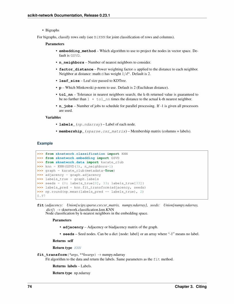
scikit-network Documentation, Release 0.23.1
• Bigraphs
For bigraphs, classify rows only (see BiKNN for joint classification of rows and columns).
Parameters
• embedding_method – Which algorithm to use to project the nodes in vector space. De-fault is GSVD.
• n_neighbors – Number of nearest neighbors to consider.
• factor_distance – Power weighting factor 𝛼 applied to the distance to each neighbor.Neighbor at distance :math:d has weight 1/𝑑𝛼. Default is 2.
• leaf_size – Leaf size passed to KDTree.
• p – Which Minkowski p-norm to use. Default is 2 (Euclidean distance).
• tol_nn – Tolerance in nearest neighbors search; the k-th returned value is guaranteed tobe no further than 1 + tol_nn times the distance to the actual k-th nearest neighbor.
• n_jobs – Number of jobs to schedule for parallel processing. If -1 is given all processorsare used.
Variables
• labels_ (np.ndarray) – Label of each node.
• membership_ (sparse.csr_matrix) – Membership matrix (columns = labels).
Example
>>> from sknetwork.classification import KNN>>> from sknetwork.embedding import GSVD>>> from sknetwork.data import karate_club>>> knn = KNN(GSVD(3), n_neighbors=1)>>> graph = karate_club(metadata=True)>>> adjacency = graph.adjacency>>> labels_true = graph.labels>>> seeds = {0: labels_true[0], 33: labels_true[33]}>>> labels_pred = knn.fit_transform(adjacency, seeds)>>> np.round(np.mean(labels_pred == labels_true), 2)0.97
fit(adjacency: Union[scipy.sparse.csr.csr_matrix, numpy.ndarray], seeds: Union[numpy.ndarray,dict])→ sknetwork.classification.knn.KNNNode classification by k-nearest neighbors in the embedding space.
Parameters
• adjacency – Adjacency or biadjacency matrix of the graph.
• seeds – Seed nodes. Can be a dict {node: label} or an array where “-1” means no label.
Returns self
Return type KNN
fit_transform(*args, **kwargs)→ numpy.ndarrayFit algorithm to the data and return the labels. Same parameters as the fit method.
Returns labels – Labels.
Return type np.ndarray
74 Chapter 3. Citing
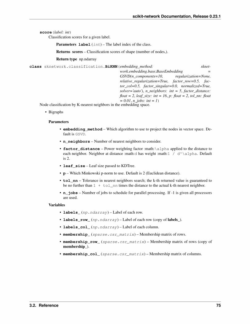
scikit-network Documentation, Release 0.23.1
score(label: int)Classification scores for a given label.
Parameters label (int) – The label index of the class.
Returns scores – Classification scores of shape (number of nodes,).
Return type np.ndarray
class sknetwork.classification.BiKNN(embedding_method: sknet-work.embedding.base.BaseEmbedding =GSVD(n_components=10, regularization=None,relative_regularization=True, factor_row=0.5, fac-tor_col=0.5, factor_singular=0.0, normalized=True,solver='auto'), n_neighbors: int = 5, factor_distance:float = 2, leaf_size: int = 16, p: float = 2, tol_nn: float= 0.01, n_jobs: int = 1)
Node classification by K-nearest neighbors in the embedding space.
• Bigraphs
Parameters
• embedding_method – Which algorithm to use to project the nodes in vector space. De-fault is GSVD.
• n_neighbors – Number of nearest neighbors to consider.
• factor_distance – Power weighting factor :math:\alpha applied to the distance toeach neighbor. Neighbor at distance :math:d has weight :math:1 / d^\alpha. Defaultis 2.
• leaf_size – Leaf size passed to KDTree.
• p – Which Minkowski p-norm to use. Default is 2 (Euclidean distance).
• tol_nn – Tolerance in nearest neighbors search; the k-th returned value is guaranteed tobe no further than 1 + tol_nn times the distance to the actual k-th nearest neighbor.
• n_jobs – Number of jobs to schedule for parallel processing. If -1 is given all processorsare used.
Variables
• labels_ (np.ndarray) – Label of each row.
• labels_row_ (np.ndarray) – Label of each row (copy of labels_).
• labels_col_ (np.ndarray) – Label of each column.
• membership_ (sparse.csr_matrix) – Membership matrix of rows.
• membership_row_ (sparse.csr_matrix) – Membership matrix of rows (copy ofmembership_).
• membership_col_ (sparse.csr_matrix) – Membership matrix of columns.
3.2. Reference 75
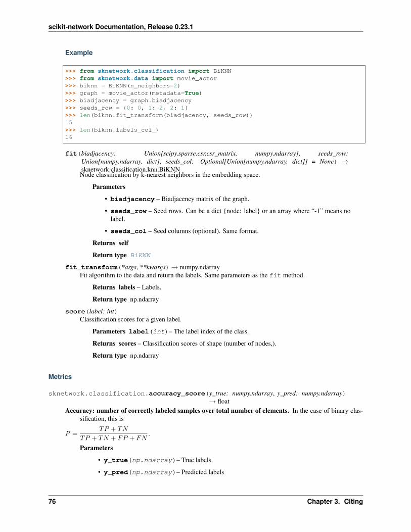
scikit-network Documentation, Release 0.23.1
Example
>>> from sknetwork.classification import BiKNN>>> from sknetwork.data import movie_actor>>> biknn = BiKNN(n_neighbors=2)>>> graph = movie_actor(metadata=True)>>> biadjacency = graph.biadjacency>>> seeds_row = {0: 0, 1: 2, 2: 1}>>> len(biknn.fit_transform(biadjacency, seeds_row))15>>> len(biknn.labels_col_)16
fit(biadjacency: Union[scipy.sparse.csr.csr_matrix, numpy.ndarray], seeds_row:Union[numpy.ndarray, dict], seeds_col: Optional[Union[numpy.ndarray, dict]] = None) →sknetwork.classification.knn.BiKNNNode classification by k-nearest neighbors in the embedding space.
Parameters
• biadjacency – Biadjacency matrix of the graph.
• seeds_row – Seed rows. Can be a dict {node: label} or an array where “-1” means nolabel.
• seeds_col – Seed columns (optional). Same format.
Returns self
Return type BiKNN
fit_transform(*args, **kwargs)→ numpy.ndarrayFit algorithm to the data and return the labels. Same parameters as the fit method.
Returns labels – Labels.
Return type np.ndarray
score(label: int)Classification scores for a given label.
Parameters label (int) – The label index of the class.
Returns scores – Classification scores of shape (number of nodes,).
Return type np.ndarray
Metrics
sknetwork.classification.accuracy_score(y_true: numpy.ndarray, y_pred: numpy.ndarray)→ float
Accuracy: number of correctly labeled samples over total number of elements. In the case of binary clas-sification, this is
𝑃 =𝑇𝑃 + 𝑇𝑁
𝑇𝑃 + 𝑇𝑁 + 𝐹𝑃 + 𝐹𝑁.
Parameters
• y_true (np.ndarray) – True labels.
• y_pred (np.ndarray) – Predicted labels
76 Chapter 3. Citing
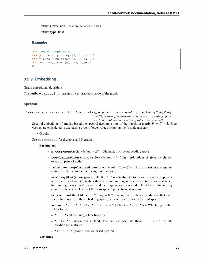
scikit-network Documentation, Release 0.23.1
Returns precision – A score between 0 and 1.
Return type float
Examples
>>> import numpy as np>>> y_true = np.array([0, 0, 1, 1])>>> y_pred = np.array([0, 0, 0, 1])>>> accuracy_score(y_true, y_pred)0.75
3.2.9 Embedding
Graph embedding algorithms.
The attribute embedding_ assigns a vector to each node of the graph.
Spectral
class sknetwork.embedding.Spectral(n_components: int = 2, regularization: Union[None, float]= 0.01, relative_regularization: bool = True, scaling: float= 0.5, normalized: bool = True, solver: str = 'auto')
Spectral embedding of graphs, based the spectral decomposition of the transition matrix 𝑃 = 𝐷−1𝐴. Eigen-vectors are considered in decreasing order of eigenvalues, skipping the first eigenvector.
• Graphs
See BiSpectral for digraphs and bigraphs.
Parameters
• n_components (int (default = 2)) – Dimension of the embedding space.
• regularization (None or float (default = 0.01)) – Add edges of given weight be-tween all pairs of nodes.
• relative_regularization (bool (default = True)) – If True, consider the regular-ization as relative to the total weight of the graph.
• scaling (float (non-negative, default = 0.5)) – Scaling factor 𝛼 so that each componentis divided by (1 − 𝜆)𝛼, with 𝜆 the corresponding eigenvalue of the transition matrix 𝑃 .Require regularization if positive and the graph is not connected. The default value 𝛼 = 1
2equalizes the energy levels of the corresponding mechanical system.
• normalized (bool (default = True)) – If True, normalize the embedding so that eachvector has norm 1 in the embedding space, i.e., each vector lies on the unit sphere.
• solver ('auto', 'halko', 'lanczos' (default = 'auto')) – Which eigenvaluesolver to use.
– 'auto' call the auto_solver function.
– 'halko': randomized method, fast but less accurate than 'lanczos' for ill-conditioned matrices.
– 'lanczos': power-iteration based method.
Variables
3.2. Reference 77
scikit-network Documentation, Release 0.23.1
• embedding_ (array, shape = (n, n_components)) – Embedding of thenodes.
• eigenvalues_ (array, shape = (n_components)) – Eigenvalues in decreas-ing order (first eigenvalue ignored).
• eigenvectors_ (array, shape = (n, n_components)) – Correspondingeigenvectors.
• regularization_ (None or float) – Regularization factor added to all pairs of nodes.
Example
>>> from sknetwork.embedding import Spectral>>> from sknetwork.data import karate_club>>> spectral = Spectral()>>> adjacency = karate_club()>>> embedding = spectral.fit_transform(adjacency)>>> embedding.shape(34, 2)
References
Belkin, M. & Niyogi, P. (2003). Laplacian Eigenmaps for Dimensionality Reduction and Data Representation,Neural computation.
fit(adjacency: Union[scipy.sparse.csr.csr_matrix, numpy.ndarray]) → sknet-work.embedding.spectral.SpectralCompute the graph embedding.
Parameters adjacency – Adjacency matrix of the graph (symmetric matrix).
Returns self
Return type Spectral
fit_transform(*args, **kwargs)→ numpy.ndarrayFit to data and return the embedding. Same parameters as the fit method.
Returns embedding – Embedding.
Return type np.ndarray
predict(adjacency_vectors: Union[scipy.sparse.csr.csr_matrix, numpy.ndarray])→ numpy.ndarrayPredict the embedding of new nodes, defined by their adjacency vectors.
Parameters adjacency_vectors – Adjacency vectors of nodes. Array of shape (n_col,)(single vector) or (n_vectors, n_col)
Returns embedding_vectors – Embedding of the nodes.
Return type np.ndarray
class sknetwork.embedding.BiSpectral(n_components: int = 2, regularization: Union[None,float] = 0.01, relative_regularization: bool = True, scal-ing: float = 0.5, normalized: bool = True, solver: str ='auto')
Spectral embedding of bipartite and directed graphs, based the spectral embedding of the corresponding undi-rected graph, with adjacency matrix:
78 Chapter 3. Citing
scikit-network Documentation, Release 0.23.1
𝐴 =
[0 𝐵𝐵𝑇 0
]where 𝐵 is the biadjacency matrix of the bipartite graph or the adjacency matrix of the directed graph.
• Digraphs
• Bigraphs
Parameters
• n_components (int (default = 2)) – Dimension of the embedding space.
• regularization (None or float (default = 0.01)) – Add edges of given weight be-tween all pairs of nodes.
• relative_regularization (bool (default = True)) – If True, consider the regular-ization as relative to the total weight of the graph.
• scaling (float (non-negative, default = 0.5)) – Scaling factor 𝛼 so that each componentis divided by (1 − 𝜆)𝛼, with 𝜆 the corresponding eigenvalue of the transition matrix 𝑃 .Require regularization if positive and the graph is not connected. The default value 𝛼 = 1
2equalizes the energy levels of the corresponding mechanical system.
• normalized (bool (default = True)) – If True, normalized the embedding so that eachvector has norm 1 in the embedding space, i.e., each vector lies on the unit sphere.
• solver ('auto', 'halko', 'lanczos' (default = 'auto')) – Which eigenvaluesolver to use.
– 'auto' call the auto_solver function.
– 'halko': randomized method, fast but less accurate than 'lanczos' for ill-conditioned matrices.
– 'lanczos': power-iteration based method.
Variables
• embedding_ (array, shape = (n_row, n_components)) – Embedding ofthe rows.
• embedding_row_ (array, shape = (n_row, n_components)) – Embed-ding of the rows (copy of embedding_).
• embedding_col_ (array, shape = (n_col, n_components)) – Embeddingof the columns.
• eigenvalues_ (array, shape = (n_components)) – Eigenvalues in increas-ing order (first eigenvalue ignored).
• eigenvectors_ (array, shape = (n, n_components)) – Correspondingeigenvectors.
• regularization_ (None or float) – Regularization factor added to all pairs of nodes.
3.2. Reference 79
scikit-network Documentation, Release 0.23.1
Example
>>> from sknetwork.embedding import BiSpectral>>> from sknetwork.data import movie_actor>>> bispectral = BiSpectral()>>> biadjacency = movie_actor()>>> embedding = bispectral.fit_transform(biadjacency)>>> embedding.shape(15, 2)
References
Belkin, M. & Niyogi, P. (2003). Laplacian Eigenmaps for Dimensionality Reduction and Data Representation,Neural computation.
fit(biadjacency: Union[scipy.sparse.csr.csr_matrix, numpy.ndarray]) → sknet-work.embedding.spectral.BiSpectralSpectral embedding of the bipartite graph considered as undirected, with adjacency matrix:
𝐴 =
[0 𝐵𝐵𝑇 0
]where 𝐵 is the biadjacency matrix (or the adjacency matrix of a directed graph).
Parameters biadjacency – Biadjacency matrix of the graph.
Returns self
Return type BiSpectral
fit_transform(*args, **kwargs)→ numpy.ndarrayFit to data and return the embedding. Same parameters as the fit method.
Returns embedding – Embedding.
Return type np.ndarray
predict(adjacency_vectors: Union[scipy.sparse.csr.csr_matrix, numpy.ndarray])→ numpy.ndarrayPredict the embedding of new rows, defined by their adjacency vectors.
Parameters adjacency_vectors – Adjacency vectors of nodes. Array of shape (n_col,)(single vector) or (n_vectors, n_col)
Returns embedding_vectors – Embedding of the nodes.
Return type np.ndarray
class sknetwork.embedding.LaplacianEmbedding(n_components: int = 2, regulariza-tion: Union[None, float] = 0.01, rela-tive_regularization: bool = True, scaling:float = 0.5, normalized: bool = True,solver: str = 'auto')
Spectral embedding of graphs, based the spectral decomposition of the Laplacian matrix 𝐿 = 𝐷 − 𝐴. Eigen-vectors are considered in increasing order of eigenvalues, skipping the first eigenvector.
• Graphs
Parameters
• n_components (int (default = 2)) – Dimension of the embedding space.
80 Chapter 3. Citing
scikit-network Documentation, Release 0.23.1
• regularization (None or float (default = 0.01)) – Add edges of given weight be-tween all pairs of nodes.
• relative_regularization (bool (default = True)) – If True, consider the regular-ization as relative to the total weight of the graph.
• scaling (float (non-negative, default = 0.5)) – Scaling factor 𝛼 so that each componentis divided by 𝜆𝛼, with 𝜆 the corresponding eigenvalue of the Laplacian matrix 𝐿. Requireregularization if positive and the graph is not connected. The default value 𝛼 = 1
2 equalizesthe energy levels of the corresponding mechanical system.
• normalized (bool (default = True)) – If True, normalize the embedding so that eachvector has norm 1 in the embedding space, i.e., each vector lies on the unit sphere.
• solver ('auto', 'halko', 'lanczos' (default = 'auto')) – Which eigenvaluesolver to use.
– 'auto' call the auto_solver function.
– 'halko': randomized method, fast but less accurate than 'lanczos' for ill-conditioned matrices.
– 'lanczos': power-iteration based method.
Variables
• embedding_ (array, shape = (n, n_components)) – Embedding of thenodes.
• eigenvalues_ (array, shape = (n_components)) – Eigenvalues in increas-ing order (first eigenvalue ignored).
• eigenvectors_ (array, shape = (n, n_components)) – Correspondingeigenvectors.
• regularization_ (None or float) – Regularization factor added to all pairs of nodes.
Example
>>> from sknetwork.embedding import LaplacianEmbedding>>> from sknetwork.data import karate_club>>> laplacian = LaplacianEmbedding()>>> adjacency = karate_club()>>> embedding = laplacian.fit_transform(adjacency)>>> embedding.shape(34, 2)
References
Belkin, M. & Niyogi, P. (2003). Laplacian Eigenmaps for Dimensionality Reduction and Data Representation,Neural computation.
fit(adjacency: Union[scipy.sparse.csr.csr_matrix, numpy.ndarray]) → sknet-work.embedding.spectral.LaplacianEmbeddingCompute the graph embedding.
Parameters adjacency – Adjacency matrix of the graph (symmetric matrix).
Returns self
3.2. Reference 81
scikit-network Documentation, Release 0.23.1
Return type LaplacianEmbedding
fit_transform(*args, **kwargs)→ numpy.ndarrayFit to data and return the embedding. Same parameters as the fit method.
Returns embedding – Embedding.
Return type np.ndarray
SVD
class sknetwork.embedding.SVD(n_components=2, regularization: Optional[float] = None, rel-ative_regularization: bool = True, factor_singular: float =0.0, normalized: bool = False, solver: Union[str, sknet-work.linalg.svd_solver.SVDSolver] = 'auto')
Graph embedding by Singular Value Decomposition of the adjacency or biadjacency matrix.
• Graphs
• Digraphs
• Bigraphs
Parameters
• n_components (int) – Dimension of the embedding.
• regularization (None or float (default = None)) – Implicitly add edges of givenweight between all pairs of nodes.
• relative_regularization (bool (default = True)) – If True, consider the regular-ization as relative to the total weight of the graph.
• factor_singular (float (default = 0.)) – Power factor 𝛼 applied to the sin-gular values on right singular vectors. The embedding of rows and columns are respectively𝑈Σ1−𝛼 and 𝑉 Σ𝛼 where:
– 𝑈 is the matrix of left singular vectors, shape (n_row, n_components)
– 𝑉 is the matrix of right singular vectors, shape (n_col, n_components)
– Σ is the diagonal matrix of singular values, shape (n_components, n_components)
• normalized (bool (default = False)) – If True, normalized the embedding so that eachvector has norm 1 in the embedding space, i.e., each vector lies on the unit sphere.
• solver ('auto', 'halko', 'lanczos' or SVDSolver) – Which singular valuesolver to use.
– 'auto': call the auto_solver function.
– 'halko': randomized method, fast but less accurate than 'lanczos' for ill-conditioned matrices.
– 'lanczos': power-iteration based method.
– SVDSolver: custom solver.
Variables
• embedding_ (np.ndarray, shape = (n_row, n_components)) – Embed-ding of the rows.
82 Chapter 3. Citing
scikit-network Documentation, Release 0.23.1
• embedding_row_ (np.ndarray, shape = (n_row, n_components)) –Embedding of the rows (copy of embedding_).
• embedding_col_ (np.ndarray, shape = (n_col, n_components)) –Embedding of the columns.
• singular_values_ (np.ndarray, shape = (n_components)) – Singularvalues.
• singular_vectors_left_ (np.ndarray, shape = (n_row,n_components)) – Left singular vectors.
• singular_vectors_right_ (np.ndarray, shape = (n_col,n_components)) – Right singular vectors.
• regularization_ (None or float) – Regularization factor added to all pairs of nodes.
Example
>>> from sknetwork.embedding import SVD>>> from sknetwork.data import karate_club>>> svd = SVD()>>> adjacency = karate_club()>>> embedding = svd.fit_transform(adjacency)>>> embedding.shape(34, 2)
References
Abdi, H. (2007). Singular value decomposition (SVD) and generalized singular value decomposition. Encyclo-pedia of measurement and statistics.
fit(adjacency: Union[scipy.sparse.csr.csr_matrix, numpy.ndarray]) → sknet-work.embedding.svd.GSVDCompute the embedding of the graph.
Parameters adjacency – Adjacency or biadjacency matrix of the graph.
Returns self
Return type GSVD
fit_transform(*args, **kwargs)→ numpy.ndarrayFit to data and return the embedding. Same parameters as the fit method.
Returns embedding – Embedding.
Return type np.ndarray
predict(adjacency_vectors: Union[scipy.sparse.csr.csr_matrix, numpy.ndarray])→ numpy.ndarrayPredict the embedding of new rows, defined by their adjacency vectors.
Parameters adjacency_vectors – Adjacency vectors of nodes. Array of shape (n_col,)(single vector) or (n_vectors, n_col)
Returns embedding_vectors – Embedding of the nodes.
Return type np.ndarray
3.2. Reference 83
scikit-network Documentation, Release 0.23.1
GSVD
class sknetwork.embedding.GSVD(n_components=2, regularization: Optional[float] = None,relative_regularization: bool = True, factor_row: float =0.5, factor_col: float = 0.5, factor_singular: float =0.0, normalized: bool = True, solver: Union[str, sknet-work.linalg.svd_solver.SVDSolver] = 'auto')
Graph embedding by Generalized Singular Value Decomposition of the adjacency or biadjacency matrix 𝐴. Thisis equivalent to the Singular Value Decomposition of the matrix 𝐷−𝛼1
1 𝐴𝐷−𝛼22 where 𝐷1, 𝐷2 are the diagonal
matrices of row weights and columns weights, respectively, and 𝛼1, 𝛼2 are parameters.
• Graphs
• Digraphs
• Bigraphs
Parameters
• n_components (int) – Dimension of the embedding.
• regularization (None or float (default = None)) – Implicitly add edges of givenweight between all pairs of nodes.
• relative_regularization (bool (default = True)) – If True, consider the regular-ization as relative to the total weight of the graph.
• factor_row (float (default = 0.5)) – Power factor 𝛼1 applied to the diagonalmatrix of row weights.
• factor_col (float (default = 0.5)) – Power factor 𝛼2 applied to the diagonalmatrix of column weights.
• factor_singular (float (default = 0.)) – Parameter 𝛼 applied to the singu-lar values on right singular vectors. The embedding of rows and columns are respectively𝐷−𝛼1
1 𝑈Σ1−𝛼 and 𝐷−𝛼22 𝑉 Σ𝛼 where:
– 𝑈 is the matrix of left singular vectors, shape (n_row, n_components)
– 𝑉 is the matrix of right singular vectors, shape (n_col, n_components)
– Σ is the diagonal matrix of singular values, shape (n_components, n_components)
• normalized (bool (default = True)) – If True, normalized the embedding so that eachvector has norm 1 in the embedding space, i.e., each vector lies on the unit sphere.
• solver ('auto', 'halko', 'lanczos' or SVDSolver) – Which singular valuesolver to use.
– 'auto': call the auto_solver function.
– 'halko': randomized method, fast but less accurate than 'lanczos' for ill-conditioned matrices.
– 'lanczos': power-iteration based method.
– SVDSolver: custom solver.
Variables
• embedding_ (np.ndarray, shape = (n1, n_components)) – Embedding ofthe rows.
• embedding_row_ (np.ndarray, shape = (n1, n_components)) – Embed-ding of the rows (copy of embedding_).
84 Chapter 3. Citing
scikit-network Documentation, Release 0.23.1
• embedding_col_ (np.ndarray, shape = (n2, n_components)) – Embed-ding of the columns.
• singular_values_ (np.ndarray, shape = (n_components)) – Singularvalues.
• singular_vectors_left_ (np.ndarray, shape = (n_row,n_components)) – Left singular vectors.
• singular_vectors_right_ (np.ndarray, shape = (n_col,n_components)) – Right singular vectors.
• regularization_ (None or float) – Regularization factor added to all pairs of nodes.
• weights_col_ (np.ndarray, shape = (n2)) – Weights applied to columns.
Example
>>> from sknetwork.embedding import GSVD>>> from sknetwork.data import karate_club>>> gsvd = GSVD()>>> adjacency = karate_club()>>> embedding = gsvd.fit_transform(adjacency)>>> embedding.shape(34, 2)
References
Abdi, H. (2007). Singular value decomposition (SVD) and generalized singular value decomposition. Encyclo-pedia of measurement and statistics, 907-912.
fit(adjacency: Union[scipy.sparse.csr.csr_matrix, numpy.ndarray]) → sknet-work.embedding.svd.GSVDCompute the embedding of the graph.
Parameters adjacency – Adjacency or biadjacency matrix of the graph.
Returns self
Return type GSVD
fit_transform(*args, **kwargs)→ numpy.ndarrayFit to data and return the embedding. Same parameters as the fit method.
Returns embedding – Embedding.
Return type np.ndarray
predict(adjacency_vectors: Union[scipy.sparse.csr.csr_matrix, numpy.ndarray])→ numpy.ndarrayPredict the embedding of new rows, defined by their adjacency vectors.
Parameters adjacency_vectors – Adjacency vectors of nodes. Array of shape (n_col,)(single vector) or (n_vectors, n_col)
Returns embedding_vectors – Embedding of the nodes.
Return type np.ndarray
3.2. Reference 85
scikit-network Documentation, Release 0.23.1
PCA
class sknetwork.embedding.PCA(n_components=2, normalized: bool = False, solver: Union[str,sknetwork.linalg.svd_solver.SVDSolver] = 'auto')
Graph embedding by Principal Component Analysis of the adjacency or biadjacency matrix.
• Graphs
• Digraphs
• Bigraphs
Parameters
• n_components (int) – Dimension of the embedding.
• normalized (bool (default = False)) – If True, normalized the embedding so that eachvector has norm 1 in the embedding space, i.e., each vector lies on the unit sphere.
• solver ('auto', 'halko', 'lanczos' or SVDSolver) – Which singular valuesolver to use.
– 'auto': call the auto_solver function.
– 'halko': randomized method, fast but less accurate than 'lanczos' for ill-conditioned matrices.
– 'lanczos': power-iteration based method.
– SVDSolver: custom solver.
Variables
• embedding_ (np.ndarray, shape = (n_row, n_components)) – Embed-ding of the rows.
• embedding_row_ (np.ndarray, shape = (n_row, n_components)) –Embedding of the rows (copy of embedding_).
• embedding_col_ (np.ndarray, shape = (n_col, n_components)) –Embedding of the columns.
• singular_values_ (np.ndarray, shape = (n_components)) – Singularvalues.
• singular_vectors_left_ (np.ndarray, shape = (n_row,n_components)) – Left singular vectors.
• singular_vectors_right_ (np.ndarray, shape = (n_col,n_components)) – Right singular vectors.
• regularization_ (None or float) – Regularization factor added to all pairs of nodes.
86 Chapter 3. Citing
scikit-network Documentation, Release 0.23.1
Example
>>> from sknetwork.embedding import PCA>>> from sknetwork.data import karate_club>>> pca = PCA()>>> adjacency = karate_club()>>> embedding = pca.fit_transform(adjacency)>>> embedding.shape(34, 2)
References
Jolliffe, I.T. (2002). Principal Component Analysis Series: Springer Series in Statistics.
fit(adjacency: Union[scipy.sparse.csr.csr_matrix, numpy.ndarray]) → sknet-work.embedding.svd.PCACompute the embedding of the graph.
Parameters adjacency – Adjacency or biadjacency matrix of the graph.
Returns self
Return type PCA
fit_transform(*args, **kwargs)→ numpy.ndarrayFit to data and return the embedding. Same parameters as the fit method.
Returns embedding – Embedding.
Return type np.ndarray
predict(adjacency_vectors: Union[scipy.sparse.csr.csr_matrix, numpy.ndarray])→ numpy.ndarrayPredict the embedding of new rows, defined by their adjacency vectors.
Parameters adjacency_vectors – Adjacency vectors of nodes. Array of shape (n_col,)(single vector) or (n_vectors, n_col)
Returns embedding_vectors – Embedding of the nodes.
Return type np.ndarray
Random Projection
class sknetwork.embedding.RandomProjection(n_components: int = 2, alpha: float = 0.5,n_iter: int = 3, random_walk: bool = False,normalized: bool = True, random_state: Op-tional[int] = None)
Embedding of graphs based the random projection of the adjacency matrix:
(𝐼 + 𝛼𝐴 + ... + (𝛼𝐴)𝐾)𝐺
where 𝐴 is the adjacency matrix, 𝐺 is a random Gaussian matrix, 𝛼 is some smoothing factor and 𝐾 non-negative integer.
• Graphs
• Digraphs
Parameters
• n_components (int (default = 2)) – Dimension of the embedding space.
3.2. Reference 87
scikit-network Documentation, Release 0.23.1
• alpha (float (default = 0.5)) – Smoothing parameter.
• n_iter (int (default = 3)) – Number of power iterations of the adjacency matrix.
• random_walk (bool (default = False)) – If True, use the transition matrix of the ran-dom walk, 𝑃 = 𝐷−1𝐴, instead of the adjacency matrix.
• normalized (bool (default = True)) – If True, normalize the embedding so that eachvector has norm 1 in the embedding space, i.e., each vector lies on the unit sphere.
• random_state (int, optional) – Seed used by the random number generator.
Variables embedding_ (array, shape = (n, n_components)) – Embedding of thenodes.
Example
>>> from sknetwork.embedding import RandomProjection>>> from sknetwork.data import karate_club>>> projection = RandomProjection()>>> adjacency = karate_club()>>> embedding = projection.fit_transform(adjacency)>>> embedding.shape(34, 2)
References
Zhang, Z., Cui, P., Li, H., Wang, X., & Zhu, W. (2018). Billion-scale network embedding with iterative randomprojection, ICDM.
fit(adjacency: Union[scipy.sparse.csr.csr_matrix, numpy.ndarray]) → sknet-work.embedding.random_projection.RandomProjectionCompute the graph embedding.
Parameters adjacency – Adjacency matrix of the graph.
Returns self
Return type RandomProjection
fit_transform(*args, **kwargs)→ numpy.ndarrayFit to data and return the embedding. Same parameters as the fit method.
Returns embedding – Embedding.
Return type np.ndarray
class sknetwork.embedding.BiRandomProjection(n_components: int = 2, alpha: float = 0.5,n_iter: int = 3, random_walk: bool = False,normalized: bool = True)
Embedding of bipartite graphs, based the random projection of the corresponding adjacency matrix:
𝐴 =
[0 𝐵𝐵𝑇 0
]where 𝐵 is the biadjacency matrix of the bipartite graph.
• Bigraphs
Parameters
88 Chapter 3. Citing
scikit-network Documentation, Release 0.23.1
• n_components (int (default = 2)) – Dimension of the embedding space.
• alpha (float (default = 0.5)) – Smoothing parameter.
• n_iter (int (default = 3)) – Number of power iterations of the adjacency matrix.
• random_walk (bool (default = False)) – If True, use the transition matrix of the ran-dom walk, 𝑃 = 𝐷−1𝐴, instead of the adjacency matrix.
• normalized (bool (default = True)) – If True, normalized the embedding so that eachvector has norm 1 in the embedding space, i.e., each vector lies on the unit sphere.
Variables
• embedding_ (array, shape = (n_row, n_components)) – Embedding ofthe rows.
• embedding_row_ (array, shape = (n_row, n_components)) – Embed-ding of the rows (copy of embedding_).
• embedding_col_ (array, shape = (n_col, n_components)) – Embeddingof the columns.
Example
>>> from sknetwork.embedding import BiRandomProjection>>> from sknetwork.data import movie_actor>>> biprojection = BiRandomProjection()>>> biadjacency = movie_actor()>>> embedding = biprojection.fit_transform(biadjacency)>>> embedding.shape(15, 2)
References
Zhang, Z., Cui, P., Li, H., Wang, X., & Zhu, W. (2018). Billion-scale network embedding with iterative randomprojection, ICDM.
fit(biadjacency: Union[scipy.sparse.csr.csr_matrix, numpy.ndarray]) → sknet-work.embedding.random_projection.BiRandomProjectionCompute the embedding.
Parameters biadjacency – Biadjacency matrix of the graph.
Returns self
Return type BiRandomProjection
fit_transform(*args, **kwargs)→ numpy.ndarrayFit to data and return the embedding. Same parameters as the fit method.
Returns embedding – Embedding.
Return type np.ndarray
3.2. Reference 89
scikit-network Documentation, Release 0.23.1
Louvain
class sknetwork.embedding.LouvainEmbedding(resolution: float = 1, modularity: str= 'dugue', tol_optimization: float =0.001, tol_aggregation: float = 0.001,n_aggregations: int = - 1, shuffle_nodes:bool = False, random_state: Op-tional[Union[numpy.random.mtrand.RandomState,int]] = None, isolated_nodes: str = 'remove')
Embedding of graphs induced by Louvain clustering. Each component of the embedding corresponds to acluster obtained by Louvain.
Parameters
• resolution (float) – Resolution parameter.
• modularity (str) – Which objective function to maximize. Can be 'dugue','newman' or 'potts'.
• tol_optimization – Minimum increase in the objective function to enter a new opti-mization pass.
• tol_aggregation – Minimum increase in the objective function to enter a new aggre-gation pass.
• n_aggregations – Maximum number of aggregations. A negative value is interpretedas no limit.
• shuffle_nodes – Enables node shuffling before optimization.
• random_state – Random number generator or random seed. If None, numpy.random isused.
• isolated_nodes (str) – What to do with isolated nodes. Can be 'remove' (default),'merge' or 'keep'.
Variables embedding_ (array, shape = (n, n_components)) – Embedding of thenodes.
Example
>>> from sknetwork.embedding import LouvainEmbedding>>> from sknetwork.data import karate_club>>> louvain = LouvainEmbedding()>>> adjacency = karate_club()>>> embedding = louvain.fit_transform(adjacency)>>> embedding.shape(34, 4)
fit(adjacency: scipy.sparse.csr.csr_matrix)Embedding of bipartite graphs from a clustering obtained with Louvain.
Parameters adjacency – Adjacency matrix of the graph.
Returns self
Return type BiLouvainEmbedding
fit_transform(*args, **kwargs)→ numpy.ndarrayFit to data and return the embedding. Same parameters as the fit method.
90 Chapter 3. Citing
scikit-network Documentation, Release 0.23.1
Returns embedding – Embedding.
Return type np.ndarray
predict(adjacency_vectors: Union[scipy.sparse.csr.csr_matrix, numpy.ndarray])→ numpy.ndarrayPredict the embedding of new rows, defined by their adjacency vectors.
Parameters adjacency_vectors – Adjacency vectors of rows. Array of shape (n_col,)(single vector) or (n_vectors, n_col)
Returns embedding_vectors – Embedding of the nodes.
Return type np.ndarray
class sknetwork.embedding.BiLouvainEmbedding(resolution: float = 1, modularity: str= 'dugue', tol_optimization: float =0.001, tol_aggregation: float = 0.001,n_aggregations: int = - 1, shuffle_nodes:bool = False, random_state: Op-tional[Union[numpy.random.mtrand.RandomState,int]] = None, isolated_nodes: str = 're-move')
Embedding of bipartite graphs induced by Louvain clustering. Each component of the embedding correspondsto a cluster obtained by Louvain.
Parameters
• resolution (float) – Resolution parameter.
• modularity (str) – Which objective function to maximize. Can be 'dugue','newman' or 'potts'.
• tol_optimization – Minimum increase in the objective function to enter a new opti-mization pass.
• tol_aggregation – Minimum increase in the objective function to enter a new aggre-gation pass.
• n_aggregations – Maximum number of aggregations. A negative value is interpretedas no limit.
• shuffle_nodes – Enables node shuffling before optimization.
• random_state – Random number generator or random seed. If None, numpy.random isused.
• isolated_nodes (str) – What to do with isolated column nodes. Can be 'remove'(default), 'merge' or 'keep'.
Variables
• embedding_ (array, shape = (n, n_components)) – Embedding of thenodes.
• embedding_row_ (array, shape = (n_row, n_components)) – Embed-ding of the rows (copy of embedding_).
• embedding_col_ (array, shape = (n_col, n_components)) – Embeddingof the columns.
• labels_row_ (np.ndarray) – Labels of the rows (used to build the embedding of thecolumns).
• labels_col_ (np.ndarray) – Labels of the columns (used to build the embedding ofthe rows).
3.2. Reference 91
scikit-network Documentation, Release 0.23.1
Example
>>> from sknetwork.embedding import BiLouvainEmbedding>>> from sknetwork.data import movie_actor>>> bilouvain = BiLouvainEmbedding()>>> biadjacency = movie_actor()>>> embedding = bilouvain.fit_transform(biadjacency)>>> embedding.shape(15, 4)
fit(biadjacency: scipy.sparse.csr.csr_matrix)Embedding of bipartite graphs from the clustering obtained with Louvain.
Parameters biadjacency – Biadjacency matrix of the graph.
Returns self
Return type BiLouvainEmbedding
fit_transform(*args, **kwargs)→ numpy.ndarrayFit to data and return the embedding. Same parameters as the fit method.
Returns embedding – Embedding.
Return type np.ndarray
predict(adjacency_vectors: Union[scipy.sparse.csr.csr_matrix, numpy.ndarray])→ numpy.ndarrayPredict the embedding of new rows, defined by their adjacency vectors.
Parameters adjacency_vectors – Adjacency vectors of rows. Array of shape (n_col,)(single vector) or (n_vectors, n_col)
Returns embedding_vectors – Embedding of the nodes.
Return type np.ndarray
Hierarchical Louvain
class sknetwork.embedding.HLouvainEmbedding(n_components: int = 2, scale: float = 0.1,resolution: float = 1, tol_optimization:float = 0.001, tol_aggregation: float =0.001, n_aggregations: int = - 1, shuf-fle_nodes: bool = False, random_state: Op-tional[Union[numpy.random.mtrand.RandomState,int]] = None, verbose: bool = False)
Embedding of graphs based on the hierarchical Louvain algorithm with random scattering per level.
Parameters
• n_components (int) – Dimension of the embedding.
• scale (float) – Dilution factor to be applied on the random vector to be added at eachiteration of the clustering method.
• resolution – Resolution parameter.
• tol_optimization – Minimum increase in the objective function to enter a new opti-mization pass.
• tol_aggregation – Minimum increase in the objective function to enter a new aggre-gation pass.
92 Chapter 3. Citing
scikit-network Documentation, Release 0.23.1
• n_aggregations – Maximum number of aggregations. A negative value is interpretedas no limit.
• shuffle_nodes – Enables node shuffling before optimization.
• random_state – Random number generator or random seed. If None, numpy.random isused.
Variables embedding_ (array, shape = (n, n_components)) – Embedding of thenodes.
Example
>>> from sknetwork.embedding import HLouvainEmbedding>>> from sknetwork.data import karate_club>>> hlouvain = HLouvainEmbedding(n_components=3)>>> adjacency = karate_club()>>> embedding = hlouvain.fit_transform(adjacency)>>> embedding.shape(34, 3)
References
Bhowmick, A. K., Meneni, K., Danisch, M., Guillaume, J. L., & Mitra, B. (2020, January). LouvainNE:Hierarchical Louvain Method for High Quality and Scalable Network Embedding. In Proceedings of the 13thInternational Conference on Web Search and Data Mining (pp. 43-51).
fit(adjacency: Union[scipy.sparse.csr.csr_matrix, numpy.ndarray])Embedding of graphs from a clustering obtained with Louvain.
Parameters adjacency – Adjacency matrix of the graph.
Returns self
Return type LouvainNE
fit_transform(*args, **kwargs)→ numpy.ndarrayFit to data and return the embedding. Same parameters as the fit method.
Returns embedding – Embedding.
Return type np.ndarray
class sknetwork.embedding.BiHLouvainEmbedding(n_components: int = 2, scale:float = 0.1, resolution: float = 1,tol_optimization: float = 0.001,tol_aggregation: float = 0.001,n_aggregations: int = - 1, shuffle_nodes:bool = False, random_state: Op-tional[Union[numpy.random.mtrand.RandomState,int]] = None, verbose: bool = False)
Embedding of graphs based on random vectors and clustering by the Louvain method.
Parameters
• n_components (int) – Dimension of the embedding.
• scale (float) – Dilution factor to be applied on the random vector to be added at eachiteration of the clustering method.
3.2. Reference 93
scikit-network Documentation, Release 0.23.1
• resolution – Resolution parameter.
• tol_optimization – Minimum increase in the objective function to enter a new opti-mization pass.
• tol_aggregation – Minimum increase in the objective function to enter a new aggre-gation pass.
• n_aggregations – Maximum number of aggregations. A negative value is interpretedas no limit.
• shuffle_nodes – Enables node shuffling before optimization.
• random_state – Random number generator or random seed. If None, numpy.random isused.
Variables
• embedding_ (array, shape = (n_row, n_components)) – Embedding ofthe rows.
• embedding_row_ (array, shape = (n_row, n_components)) – Embed-ding of the rows (copy of embedding_).
• embedding_col_ (array, shape = (n_col, n_components)) – Embeddingof the columns.
• eigenvalues_ (array, shape = (n_components)) – Eigenvalues in increas-ing order (first eigenvalue ignored).
• eigenvectors_ (array, shape = (n, n_components)) – Correspondingeigenvectors.
• regularization_ (None or float) – Regularization factor added to all pairs of nodes.
Example
>>> from sknetwork.embedding import BiHLouvainEmbedding>>> from sknetwork.data import movie_actor>>> bihlouvain = BiHLouvainEmbedding()>>> biadjacency = movie_actor()>>> embedding = bihlouvain.fit_transform(biadjacency)>>> embedding.shape(15, 2)
References
Belkin, M. & Niyogi, P. (2003). Laplacian Eigenmaps for Dimensionality Reduction and Data Representation,Neural computation.
fit(biadjacency: Union[scipy.sparse.csr.csr_matrix, numpy.ndarray]) → sknet-work.embedding.louvain_hierarchy.BiHLouvainEmbeddingEmbedding of graphs from a clustering obtained with Louvain.
Parameters biadjacency – Biadjacency matrix of the graph.
Returns self
Return type BiLouvainNE
94 Chapter 3. Citing

scikit-network Documentation, Release 0.23.1
fit_transform(*args, **kwargs)→ numpy.ndarrayFit to data and return the embedding. Same parameters as the fit method.
Returns embedding – Embedding.
Return type np.ndarray
Force Atlas
class sknetwork.embedding.ForceAtlas(n_components: int = 2, n_iter: int = 50, approx_radius:float = - 1, lin_log: bool = False, gravity_factor: float= 0.01, repulsive_factor: float = 0.1, tolerance: float =0.1, speed: float = 0.1, speed_max: float = 10)
Force Atlas layout for displaying graphs.
• Graphs
• Digraphs
Parameters
• n_components (int) – Dimension of the graph layout.
• n_iter (int) – Number of iterations to update positions. If None, use the value ofself.n_iter.
• approx_radius (float) – If a positive value is provided, only the nodes within thisdistance a given node are used to compute the repulsive force.
• lin_log (bool) – If True, use lin-log mode.
• gravity_factor (float) – Gravity force scaling constant.
• repulsive_factor (float) – Repulsive force scaling constant.
• tolerance (float) – Tolerance defined in the swinging constant.
• speed (float) – Speed constant.
• speed_max (float) – Constant used to impose constrain on speed.
Variables embedding_ (np.ndarray) – Layout in given dimension.
Example
>>> from sknetwork.embedding.force_atlas import ForceAtlas>>> from sknetwork.data import karate_club>>> force_atlas = ForceAtlas()>>> adjacency = karate_club()>>> embedding = force_atlas.fit_transform(adjacency)>>> embedding.shape(34, 2)
3.2. Reference 95
scikit-network Documentation, Release 0.23.1
References
Jacomy M., Venturini T., Heymann S., Bastian M. (2014). ForceAtlas2, a Continuous Graph Layout Algorithmfor Handy Network Visualization Designed for the Gephi Software. Plos One.
fit(adjacency: Union[scipy.sparse.csr.csr_matrix, numpy.ndarray], pos_init: Op-tional[numpy.ndarray] = None, n_iter: Optional[int] = None) → sknet-work.embedding.force_atlas.ForceAtlasCompute layout.
Parameters
• adjacency – Adjacency matrix of the graph, treated as undirected.
• pos_init – Position to start with. Random if not provided.
• n_iter (int) – Number of iterations to update positions. If None, use the value ofself.n_iter.
Returns self
Return type ForceAtlas
fit_transform(*args, **kwargs)→ numpy.ndarrayFit to data and return the embedding. Same parameters as the fit method.
Returns embedding – Embedding.
Return type np.ndarray
Spring
class sknetwork.embedding.Spring(n_components: int = 2, strength: Optional[float] = None,n_iter: int = 50, tol: float = 0.0001, approx_radius: float= - 1, position_init: str = 'random')
Spring layout for displaying small graphs.
• Graphs
• Digraphs
Parameters
• n_components (int) – Dimension of the graph layout.
• strength (float) – Intensity of the force that moves the nodes.
• n_iter (int) – Number of iterations to update positions.
• tol (float) – Minimum relative change in positions to continue updating.
• approx_radius (float) – If a positive value is provided, only the nodes within thisdistance a given node are used to compute the repulsive force.
• position_init (str) – How to initialize the layout. If ‘spectral’, use Spectral embed-ding in dimension 2, otherwise, use random initialization.
Variables embedding_ (np.ndarray) – Layout.
96 Chapter 3. Citing
scikit-network Documentation, Release 0.23.1
Example
>>> from sknetwork.embedding import Spring>>> from sknetwork.data import karate_club>>> spring = Spring()>>> adjacency = karate_club()>>> embedding = spring.fit_transform(adjacency)>>> embedding.shape(34, 2)
Notes
Simple implementation designed to display small graphs.
References
Fruchterman, T. M. J., Reingold, E. M. (1991). Graph Drawing by Force-Directed Placement. Software –Practice & Experience.
fit(adjacency: Union[scipy.sparse.csr.csr_matrix, numpy.ndarray], position_init: Op-tional[numpy.ndarray] = None, n_iter: Optional[int] = None) → sknet-work.embedding.spring.SpringCompute layout.
Parameters
• adjacency – Adjacency matrix of the graph, treated as undirected.
• position_init (np.ndarray) – Custom initial positions of the nodes. Shape mustbe (n, 2). If None, use the value of self.pos_init.
• n_iter (int) – Number of iterations to update positions. If None, use the value ofself.n_iter.
Returns self
Return type Spring
fit_transform(*args, **kwargs)→ numpy.ndarrayFit to data and return the embedding. Same parameters as the fit method.
Returns embedding – Embedding.
Return type np.ndarray
predict(adjacency_vectors: Union[scipy.sparse.csr.csr_matrix, numpy.ndarray])→ numpy.ndarrayPredict the embedding of new rows, defined by their adjacency vectors.
Parameters adjacency_vectors – Adjacency vectors of nodes. Array of shape (n_col,)(single vector) or (n_vectors, n_col)
Returns embedding_vectors – Embedding of the nodes.
Return type np.ndarray
3.2. Reference 97
scikit-network Documentation, Release 0.23.1
Metrics
sknetwork.embedding.cosine_modularity(adjacency, embedding: numpy.ndarray, embed-ding_col=None, resolution=1.0, weights='degree', re-turn_all: bool = False)
Quality metric of an embedding 𝑥 defined by:
𝑄 =∑
𝑖𝑗
(𝐴𝑖𝑗
𝑤− 𝛾
𝑤+𝑖 𝑤
−𝑗
𝑤2
)(1 + cos(𝑥𝑖, 𝑥𝑗)
2
)where
• 𝑤+𝑖 , 𝑤
−𝑖 are the out-weight, in-weight of node 𝑖 (for digraphs),
• 𝑤 = 1𝑇𝐴1 is the total weight of the graph.
For bipartite graphs with column embedding 𝑦, the metric is
𝑄 =∑
𝑖𝑗
(𝐵𝑖𝑗
𝑤− 𝛾
𝑤1,𝑖𝑤2,𝑗
𝑤2
)(1 + cos(𝑥𝑖, 𝑦𝑗)
2
)where
• 𝑤1,𝑖, 𝑤2,𝑗 are the weights of nodes 𝑖 (row) and 𝑗 (column),
• 𝑤 = 1𝑇𝐵1 is the total weight of the graph.
Parameters
• adjacency – Adjacency matrix of the graph.
• embedding – Embedding of the nodes.
• embedding_col – Embedding of the columns (for bipartite graphs).
• resolution – Resolution parameter.
• weights ('degree' or 'uniform') – Weights of the nodes.
• return_all – If True, also return fit and diversity
Returns
• modularity (float)
• fit (float, optional)
• diversity (float, optional)
Example
>>> from sknetwork.embedding import cosine_modularity>>> from sknetwork.data import karate_club>>> graph = karate_club(metadata=True)>>> adjacency = graph.adjacency>>> embedding = graph.position>>> np.round(cosine_modularity(adjacency, embedding), 2)0.35
98 Chapter 3. Citing
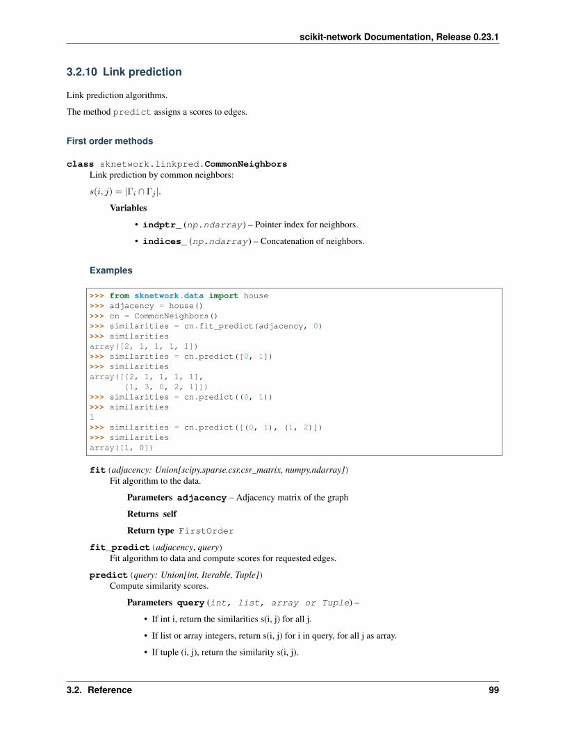
scikit-network Documentation, Release 0.23.1
3.2.10 Link prediction
Link prediction algorithms.
The method predict assigns a scores to edges.
First order methods
class sknetwork.linkpred.CommonNeighborsLink prediction by common neighbors:
𝑠(𝑖, 𝑗) = |Γ𝑖 ∩ Γ𝑗 |.
Variables
• indptr_ (np.ndarray) – Pointer index for neighbors.
• indices_ (np.ndarray) – Concatenation of neighbors.
Examples
>>> from sknetwork.data import house>>> adjacency = house()>>> cn = CommonNeighbors()>>> similarities = cn.fit_predict(adjacency, 0)>>> similaritiesarray([2, 1, 1, 1, 1])>>> similarities = cn.predict([0, 1])>>> similaritiesarray([[2, 1, 1, 1, 1],
[1, 3, 0, 2, 1]])>>> similarities = cn.predict((0, 1))>>> similarities1>>> similarities = cn.predict([(0, 1), (1, 2)])>>> similaritiesarray([1, 0])
fit(adjacency: Union[scipy.sparse.csr.csr_matrix, numpy.ndarray])Fit algorithm to the data.
Parameters adjacency – Adjacency matrix of the graph
Returns self
Return type FirstOrder
fit_predict(adjacency, query)Fit algorithm to data and compute scores for requested edges.
predict(query: Union[int, Iterable, Tuple])Compute similarity scores.
Parameters query (int, list, array or Tuple) –
• If int i, return the similarities s(i, j) for all j.
• If list or array integers, return s(i, j) for i in query, for all j as array.
• If tuple (i, j), return the similarity s(i, j).
3.2. Reference 99
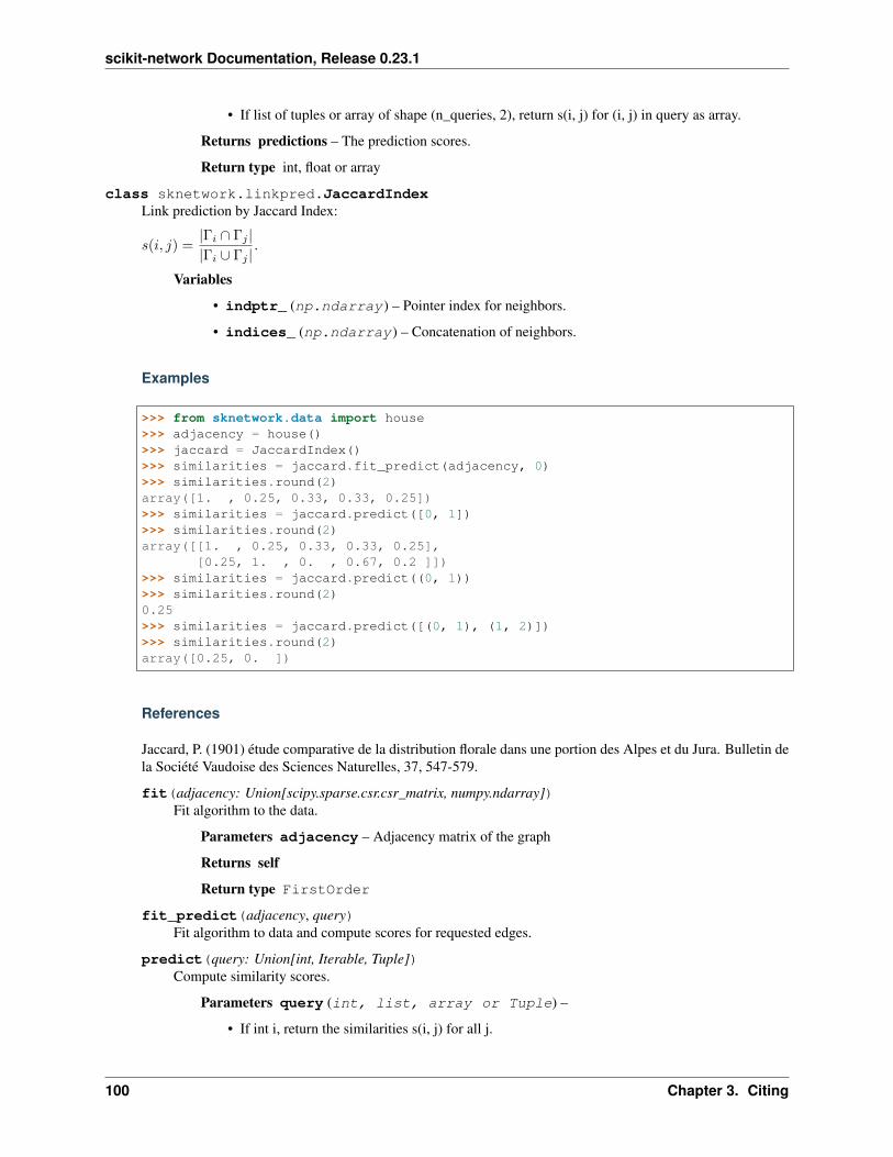
scikit-network Documentation, Release 0.23.1
• If list of tuples or array of shape (n_queries, 2), return s(i, j) for (i, j) in query as array.
Returns predictions – The prediction scores.
Return type int, float or array
class sknetwork.linkpred.JaccardIndexLink prediction by Jaccard Index:
𝑠(𝑖, 𝑗) =|Γ𝑖 ∩ Γ𝑗 ||Γ𝑖 ∪ Γ𝑗 |
.
Variables
• indptr_ (np.ndarray) – Pointer index for neighbors.
• indices_ (np.ndarray) – Concatenation of neighbors.
Examples
>>> from sknetwork.data import house>>> adjacency = house()>>> jaccard = JaccardIndex()>>> similarities = jaccard.fit_predict(adjacency, 0)>>> similarities.round(2)array([1. , 0.25, 0.33, 0.33, 0.25])>>> similarities = jaccard.predict([0, 1])>>> similarities.round(2)array([[1. , 0.25, 0.33, 0.33, 0.25],
[0.25, 1. , 0. , 0.67, 0.2 ]])>>> similarities = jaccard.predict((0, 1))>>> similarities.round(2)0.25>>> similarities = jaccard.predict([(0, 1), (1, 2)])>>> similarities.round(2)array([0.25, 0. ])
References
Jaccard, P. (1901) étude comparative de la distribution florale dans une portion des Alpes et du Jura. Bulletin dela Société Vaudoise des Sciences Naturelles, 37, 547-579.
fit(adjacency: Union[scipy.sparse.csr.csr_matrix, numpy.ndarray])Fit algorithm to the data.
Parameters adjacency – Adjacency matrix of the graph
Returns self
Return type FirstOrder
fit_predict(adjacency, query)Fit algorithm to data and compute scores for requested edges.
predict(query: Union[int, Iterable, Tuple])Compute similarity scores.
Parameters query (int, list, array or Tuple) –
• If int i, return the similarities s(i, j) for all j.
100 Chapter 3. Citing
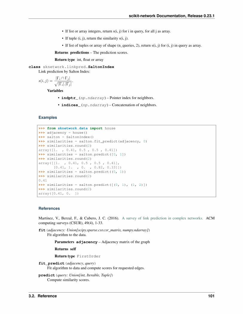
scikit-network Documentation, Release 0.23.1
• If list or array integers, return s(i, j) for i in query, for all j as array.
• If tuple (i, j), return the similarity s(i, j).
• If list of tuples or array of shape (n_queries, 2), return s(i, j) for (i, j) in query as array.
Returns predictions – The prediction scores.
Return type int, float or array
class sknetwork.linkpred.SaltonIndexLink prediction by Salton Index:
𝑠(𝑖, 𝑗) =|Γ𝑖 ∩ Γ𝑗 |√|Γ𝑖|.|Γ𝑗 |
.
Variables
• indptr_ (np.ndarray) – Pointer index for neighbors.
• indices_ (np.ndarray) – Concatenation of neighbors.
Examples
>>> from sknetwork.data import house>>> adjacency = house()>>> salton = SaltonIndex()>>> similarities = salton.fit_predict(adjacency, 0)>>> similarities.round(2)array([1. , 0.41, 0.5 , 0.5 , 0.41])>>> similarities = salton.predict([0, 1])>>> similarities.round(2)array([[1. , 0.41, 0.5 , 0.5 , 0.41],
[0.41, 1. , 0. , 0.82, 0.33]])>>> similarities = salton.predict((0, 1))>>> similarities.round(2)0.41>>> similarities = salton.predict([(0, 1), (1, 2)])>>> similarities.round(2)array([0.41, 0. ])
References
Martínez, V., Berzal, F., & Cubero, J. C. (2016). A survey of link prediction in complex networks. ACMcomputing surveys (CSUR), 49(4), 1-33.
fit(adjacency: Union[scipy.sparse.csr.csr_matrix, numpy.ndarray])Fit algorithm to the data.
Parameters adjacency – Adjacency matrix of the graph
Returns self
Return type FirstOrder
fit_predict(adjacency, query)Fit algorithm to data and compute scores for requested edges.
predict(query: Union[int, Iterable, Tuple])Compute similarity scores.
3.2. Reference 101
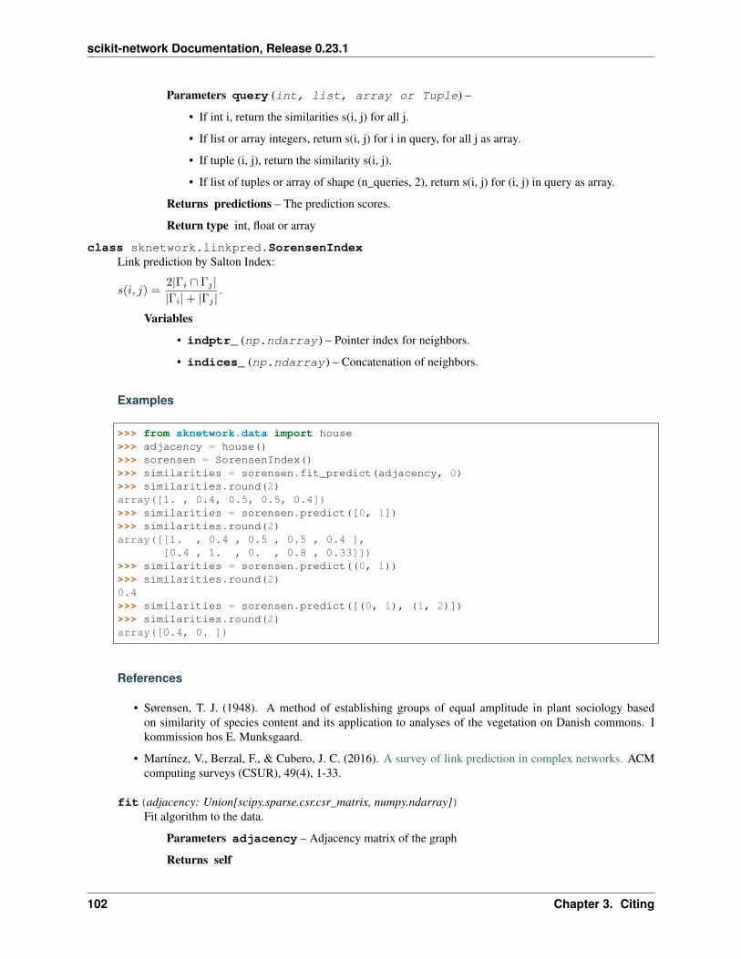
scikit-network Documentation, Release 0.23.1
Parameters query (int, list, array or Tuple) –
• If int i, return the similarities s(i, j) for all j.
• If list or array integers, return s(i, j) for i in query, for all j as array.
• If tuple (i, j), return the similarity s(i, j).
• If list of tuples or array of shape (n_queries, 2), return s(i, j) for (i, j) in query as array.
Returns predictions – The prediction scores.
Return type int, float or array
class sknetwork.linkpred.SorensenIndexLink prediction by Salton Index:
𝑠(𝑖, 𝑗) =2|Γ𝑖 ∩ Γ𝑗 ||Γ𝑖| + |Γ𝑗 |
.
Variables
• indptr_ (np.ndarray) – Pointer index for neighbors.
• indices_ (np.ndarray) – Concatenation of neighbors.
Examples
>>> from sknetwork.data import house>>> adjacency = house()>>> sorensen = SorensenIndex()>>> similarities = sorensen.fit_predict(adjacency, 0)>>> similarities.round(2)array([1. , 0.4, 0.5, 0.5, 0.4])>>> similarities = sorensen.predict([0, 1])>>> similarities.round(2)array([[1. , 0.4 , 0.5 , 0.5 , 0.4 ],
[0.4 , 1. , 0. , 0.8 , 0.33]])>>> similarities = sorensen.predict((0, 1))>>> similarities.round(2)0.4>>> similarities = sorensen.predict([(0, 1), (1, 2)])>>> similarities.round(2)array([0.4, 0. ])
References
• Sørensen, T. J. (1948). A method of establishing groups of equal amplitude in plant sociology basedon similarity of species content and its application to analyses of the vegetation on Danish commons. Ikommission hos E. Munksgaard.
• Martínez, V., Berzal, F., & Cubero, J. C. (2016). A survey of link prediction in complex networks. ACMcomputing surveys (CSUR), 49(4), 1-33.
fit(adjacency: Union[scipy.sparse.csr.csr_matrix, numpy.ndarray])Fit algorithm to the data.
Parameters adjacency – Adjacency matrix of the graph
Returns self
102 Chapter 3. Citing
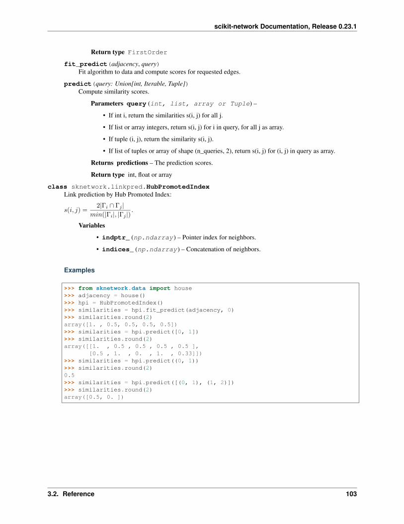
scikit-network Documentation, Release 0.23.1
Return type FirstOrder
fit_predict(adjacency, query)Fit algorithm to data and compute scores for requested edges.
predict(query: Union[int, Iterable, Tuple])Compute similarity scores.
Parameters query (int, list, array or Tuple) –
• If int i, return the similarities s(i, j) for all j.
• If list or array integers, return s(i, j) for i in query, for all j as array.
• If tuple (i, j), return the similarity s(i, j).
• If list of tuples or array of shape (n_queries, 2), return s(i, j) for (i, j) in query as array.
Returns predictions – The prediction scores.
Return type int, float or array
class sknetwork.linkpred.HubPromotedIndexLink prediction by Hub Promoted Index:
𝑠(𝑖, 𝑗) =2|Γ𝑖 ∩ Γ𝑗 |
𝑚𝑖𝑛(|Γ𝑖|, |Γ𝑗 |).
Variables
• indptr_ (np.ndarray) – Pointer index for neighbors.
• indices_ (np.ndarray) – Concatenation of neighbors.
Examples
>>> from sknetwork.data import house>>> adjacency = house()>>> hpi = HubPromotedIndex()>>> similarities = hpi.fit_predict(adjacency, 0)>>> similarities.round(2)array([1. , 0.5, 0.5, 0.5, 0.5])>>> similarities = hpi.predict([0, 1])>>> similarities.round(2)array([[1. , 0.5 , 0.5 , 0.5 , 0.5 ],
[0.5 , 1. , 0. , 1. , 0.33]])>>> similarities = hpi.predict((0, 1))>>> similarities.round(2)0.5>>> similarities = hpi.predict([(0, 1), (1, 2)])>>> similarities.round(2)array([0.5, 0. ])
3.2. Reference 103
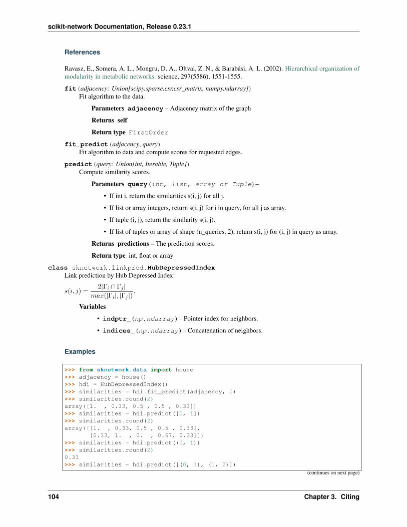
scikit-network Documentation, Release 0.23.1
References
Ravasz, E., Somera, A. L., Mongru, D. A., Oltvai, Z. N., & Barabási, A. L. (2002). Hierarchical organization ofmodularity in metabolic networks. science, 297(5586), 1551-1555.
fit(adjacency: Union[scipy.sparse.csr.csr_matrix, numpy.ndarray])Fit algorithm to the data.
Parameters adjacency – Adjacency matrix of the graph
Returns self
Return type FirstOrder
fit_predict(adjacency, query)Fit algorithm to data and compute scores for requested edges.
predict(query: Union[int, Iterable, Tuple])Compute similarity scores.
Parameters query (int, list, array or Tuple) –
• If int i, return the similarities s(i, j) for all j.
• If list or array integers, return s(i, j) for i in query, for all j as array.
• If tuple (i, j), return the similarity s(i, j).
• If list of tuples or array of shape (n_queries, 2), return s(i, j) for (i, j) in query as array.
Returns predictions – The prediction scores.
Return type int, float or array
class sknetwork.linkpred.HubDepressedIndexLink prediction by Hub Depressed Index:
𝑠(𝑖, 𝑗) =2|Γ𝑖 ∩ Γ𝑗 |
𝑚𝑎𝑥(|Γ𝑖|, |Γ𝑗 |).
Variables
• indptr_ (np.ndarray) – Pointer index for neighbors.
• indices_ (np.ndarray) – Concatenation of neighbors.
Examples
>>> from sknetwork.data import house>>> adjacency = house()>>> hdi = HubDepressedIndex()>>> similarities = hdi.fit_predict(adjacency, 0)>>> similarities.round(2)array([1. , 0.33, 0.5 , 0.5 , 0.33])>>> similarities = hdi.predict([0, 1])>>> similarities.round(2)array([[1. , 0.33, 0.5 , 0.5 , 0.33],
[0.33, 1. , 0. , 0.67, 0.33]])>>> similarities = hdi.predict((0, 1))>>> similarities.round(2)0.33>>> similarities = hdi.predict([(0, 1), (1, 2)])
(continues on next page)
104 Chapter 3. Citing
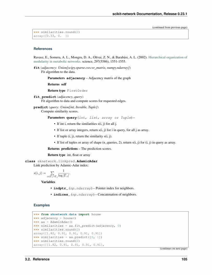
scikit-network Documentation, Release 0.23.1
(continued from previous page)
>>> similarities.round(2)array([0.33, 0. ])
References
Ravasz, E., Somera, A. L., Mongru, D. A., Oltvai, Z. N., & Barabási, A. L. (2002). Hierarchical organization ofmodularity in metabolic networks. science, 297(5586), 1551-1555.
fit(adjacency: Union[scipy.sparse.csr.csr_matrix, numpy.ndarray])Fit algorithm to the data.
Parameters adjacency – Adjacency matrix of the graph
Returns self
Return type FirstOrder
fit_predict(adjacency, query)Fit algorithm to data and compute scores for requested edges.
predict(query: Union[int, Iterable, Tuple])Compute similarity scores.
Parameters query (int, list, array or Tuple) –
• If int i, return the similarities s(i, j) for all j.
• If list or array integers, return s(i, j) for i in query, for all j as array.
• If tuple (i, j), return the similarity s(i, j).
• If list of tuples or array of shape (n_queries, 2), return s(i, j) for (i, j) in query as array.
Returns predictions – The prediction scores.
Return type int, float or array
class sknetwork.linkpred.AdamicAdarLink prediction by Adamic-Adar index:
𝑠(𝑖, 𝑗) =∑
𝑧∈Γ𝑖∩Γ𝑗
1
log |Γ𝑧|.
Variables
• indptr_ (np.ndarray) – Pointer index for neighbors.
• indices_ (np.ndarray) – Concatenation of neighbors.
Examples
>>> from sknetwork.data import house>>> adjacency = house()>>> aa = AdamicAdar()>>> similarities = aa.fit_predict(adjacency, 0)>>> similarities.round(2)array([1.82, 0.91, 0.91, 0.91, 0.91])>>> similarities = aa.predict([0, 1])>>> similarities.round(2)array([[1.82, 0.91, 0.91, 0.91, 0.91],
(continues on next page)
3.2. Reference 105
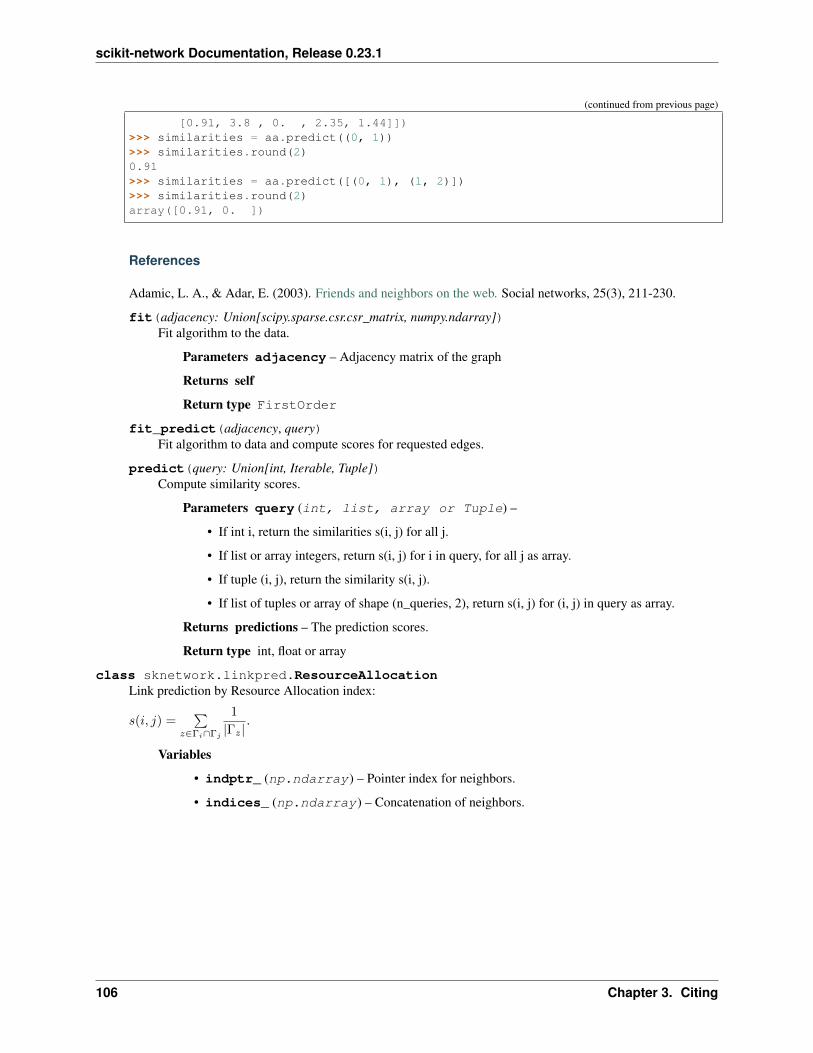
scikit-network Documentation, Release 0.23.1
(continued from previous page)
[0.91, 3.8 , 0. , 2.35, 1.44]])>>> similarities = aa.predict((0, 1))>>> similarities.round(2)0.91>>> similarities = aa.predict([(0, 1), (1, 2)])>>> similarities.round(2)array([0.91, 0. ])
References
Adamic, L. A., & Adar, E. (2003). Friends and neighbors on the web. Social networks, 25(3), 211-230.
fit(adjacency: Union[scipy.sparse.csr.csr_matrix, numpy.ndarray])Fit algorithm to the data.
Parameters adjacency – Adjacency matrix of the graph
Returns self
Return type FirstOrder
fit_predict(adjacency, query)Fit algorithm to data and compute scores for requested edges.
predict(query: Union[int, Iterable, Tuple])Compute similarity scores.
Parameters query (int, list, array or Tuple) –
• If int i, return the similarities s(i, j) for all j.
• If list or array integers, return s(i, j) for i in query, for all j as array.
• If tuple (i, j), return the similarity s(i, j).
• If list of tuples or array of shape (n_queries, 2), return s(i, j) for (i, j) in query as array.
Returns predictions – The prediction scores.
Return type int, float or array
class sknetwork.linkpred.ResourceAllocationLink prediction by Resource Allocation index:
𝑠(𝑖, 𝑗) =∑
𝑧∈Γ𝑖∩Γ𝑗
1
|Γ𝑧|.
Variables
• indptr_ (np.ndarray) – Pointer index for neighbors.
• indices_ (np.ndarray) – Concatenation of neighbors.
106 Chapter 3. Citing
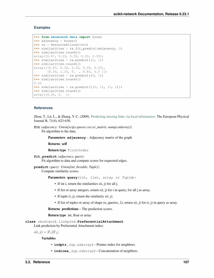
scikit-network Documentation, Release 0.23.1
Examples
>>> from sknetwork.data import house>>> adjacency = house()>>> ra = ResourceAllocation()>>> similarities = ra.fit_predict(adjacency, 0)>>> similarities.round(2)array([0.67, 0.33, 0.33, 0.33, 0.33])>>> similarities = ra.predict([0, 1])>>> similarities.round(2)array([[0.67, 0.33, 0.33, 0.33, 0.33],
[0.33, 1.33, 0. , 0.83, 0.5 ]])>>> similarities = ra.predict((0, 1))>>> similarities.round(2)0.33>>> similarities = ra.predict([(0, 1), (1, 2)])>>> similarities.round(2)array([0.33, 0. ])
References
Zhou, T., Lü, L., & Zhang, Y. C. (2009). Predicting missing links via local information. The European PhysicalJournal B, 71(4), 623-630.
fit(adjacency: Union[scipy.sparse.csr.csr_matrix, numpy.ndarray])Fit algorithm to the data.
Parameters adjacency – Adjacency matrix of the graph
Returns self
Return type FirstOrder
fit_predict(adjacency, query)Fit algorithm to data and compute scores for requested edges.
predict(query: Union[int, Iterable, Tuple])Compute similarity scores.
Parameters query (int, list, array or Tuple) –
• If int i, return the similarities s(i, j) for all j.
• If list or array integers, return s(i, j) for i in query, for all j as array.
• If tuple (i, j), return the similarity s(i, j).
• If list of tuples or array of shape (n_queries, 2), return s(i, j) for (i, j) in query as array.
Returns predictions – The prediction scores.
Return type int, float or array
class sknetwork.linkpred.PreferentialAttachmentLink prediction by Preferential Attachment index:
𝑠(𝑖, 𝑗) = |Γ𝑖||Γ𝑗 |.
Variables
• indptr_ (np.ndarray) – Pointer index for neighbors.
• indices_ (np.ndarray) – Concatenation of neighbors.
3.2. Reference 107
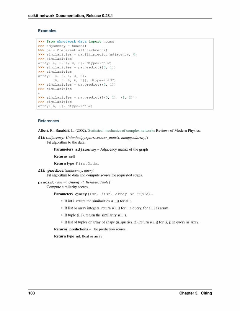
scikit-network Documentation, Release 0.23.1
Examples
>>> from sknetwork.data import house>>> adjacency = house()>>> pa = PreferentialAttachment()>>> similarities = pa.fit_predict(adjacency, 0)>>> similaritiesarray([4, 6, 4, 4, 6], dtype=int32)>>> similarities = pa.predict([0, 1])>>> similaritiesarray([[4, 6, 4, 4, 6],
[6, 9, 6, 6, 9]], dtype=int32)>>> similarities = pa.predict((0, 1))>>> similarities6>>> similarities = pa.predict([(0, 1), (1, 2)])>>> similaritiesarray([6, 6], dtype=int32)
References
Albert, R., Barabási, L. (2002). Statistical mechanics of complex networks Reviews of Modern Physics.
fit(adjacency: Union[scipy.sparse.csr.csr_matrix, numpy.ndarray])Fit algorithm to the data.
Parameters adjacency – Adjacency matrix of the graph
Returns self
Return type FirstOrder
fit_predict(adjacency, query)Fit algorithm to data and compute scores for requested edges.
predict(query: Union[int, Iterable, Tuple])Compute similarity scores.
Parameters query (int, list, array or Tuple) –
• If int i, return the similarities s(i, j) for all j.
• If list or array integers, return s(i, j) for i in query, for all j as array.
• If tuple (i, j), return the similarity s(i, j).
• If list of tuples or array of shape (n_queries, 2), return s(i, j) for (i, j) in query as array.
Returns predictions – The prediction scores.
Return type int, float or array
108 Chapter 3. Citing
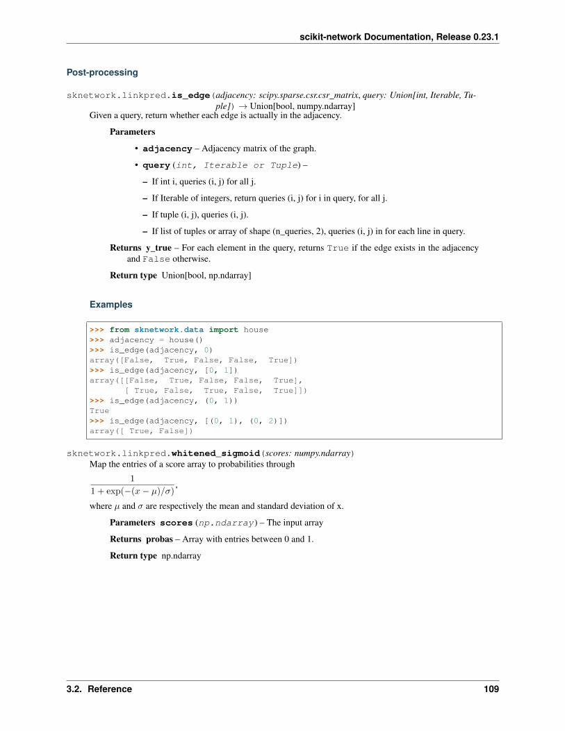
scikit-network Documentation, Release 0.23.1
Post-processing
sknetwork.linkpred.is_edge(adjacency: scipy.sparse.csr.csr_matrix, query: Union[int, Iterable, Tu-ple])→ Union[bool, numpy.ndarray]
Given a query, return whether each edge is actually in the adjacency.
Parameters
• adjacency – Adjacency matrix of the graph.
• query (int, Iterable or Tuple) –
– If int i, queries (i, j) for all j.
– If Iterable of integers, return queries (i, j) for i in query, for all j.
– If tuple (i, j), queries (i, j).
– If list of tuples or array of shape (n_queries, 2), queries (i, j) in for each line in query.
Returns y_true – For each element in the query, returns True if the edge exists in the adjacencyand False otherwise.
Return type Union[bool, np.ndarray]
Examples
>>> from sknetwork.data import house>>> adjacency = house()>>> is_edge(adjacency, 0)array([False, True, False, False, True])>>> is_edge(adjacency, [0, 1])array([[False, True, False, False, True],
[ True, False, True, False, True]])>>> is_edge(adjacency, (0, 1))True>>> is_edge(adjacency, [(0, 1), (0, 2)])array([ True, False])
sknetwork.linkpred.whitened_sigmoid(scores: numpy.ndarray)Map the entries of a score array to probabilities through
1
1 + exp(−(𝑥− 𝜇)/𝜎),
where 𝜇 and 𝜎 are respectively the mean and standard deviation of x.
Parameters scores (np.ndarray) – The input array
Returns probas – Array with entries between 0 and 1.
Return type np.ndarray
3.2. Reference 109
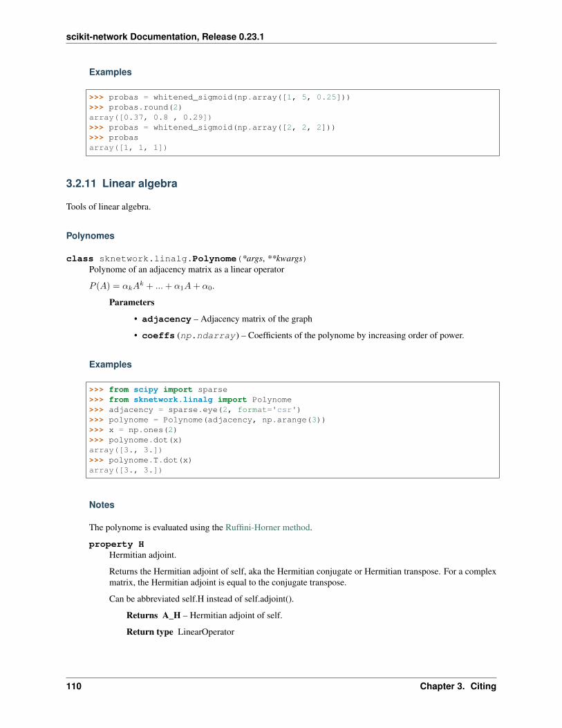
scikit-network Documentation, Release 0.23.1
Examples
>>> probas = whitened_sigmoid(np.array([1, 5, 0.25]))>>> probas.round(2)array([0.37, 0.8 , 0.29])>>> probas = whitened_sigmoid(np.array([2, 2, 2]))>>> probasarray([1, 1, 1])
3.2.11 Linear algebra
Tools of linear algebra.
Polynomes
class sknetwork.linalg.Polynome(*args, **kwargs)Polynome of an adjacency matrix as a linear operator
𝑃 (𝐴) = 𝛼𝑘𝐴𝑘 + ... + 𝛼1𝐴 + 𝛼0.
Parameters
• adjacency – Adjacency matrix of the graph
• coeffs (np.ndarray) – Coefficients of the polynome by increasing order of power.
Examples
>>> from scipy import sparse>>> from sknetwork.linalg import Polynome>>> adjacency = sparse.eye(2, format='csr')>>> polynome = Polynome(adjacency, np.arange(3))>>> x = np.ones(2)>>> polynome.dot(x)array([3., 3.])>>> polynome.T.dot(x)array([3., 3.])
Notes
The polynome is evaluated using the Ruffini-Horner method.
property HHermitian adjoint.
Returns the Hermitian adjoint of self, aka the Hermitian conjugate or Hermitian transpose. For a complexmatrix, the Hermitian adjoint is equal to the conjugate transpose.
Can be abbreviated self.H instead of self.adjoint().
Returns A_H – Hermitian adjoint of self.
Return type LinearOperator
110 Chapter 3. Citing
scikit-network Documentation, Release 0.23.1
property TTranspose this linear operator.
Returns a LinearOperator that represents the transpose of this one. Can be abbreviated self.T instead ofself.transpose().
adjoint()Hermitian adjoint.
Returns the Hermitian adjoint of self, aka the Hermitian conjugate or Hermitian transpose. For a complexmatrix, the Hermitian adjoint is equal to the conjugate transpose.
Can be abbreviated self.H instead of self.adjoint().
Returns A_H – Hermitian adjoint of self.
Return type LinearOperator
dot(x)Matrix-matrix or matrix-vector multiplication.
Parameters x (array_like) – 1-d or 2-d array, representing a vector or matrix.
Returns Ax – 1-d or 2-d array (depending on the shape of x) that represents the result of applyingthis linear operator on x.
Return type array
matmat(X)Matrix-matrix multiplication.
Performs the operation y=A*X where A is an MxN linear operator and X dense N*K matrix or ndarray.
Parameters X ({matrix, ndarray}) – An array with shape (N,K).
Returns Y – A matrix or ndarray with shape (M,K) depending on the type of the X argument.
Return type {matrix, ndarray}
Notes
This matmat wraps any user-specified matmat routine or overridden _matmat method to ensure that y hasthe correct type.
matvec(x)Matrix-vector multiplication.
Performs the operation y=A*x where A is an MxN linear operator and x is a column vector or 1-d array.
Parameters x ({matrix, ndarray}) – An array with shape (N,) or (N,1).
Returns y – A matrix or ndarray with shape (M,) or (M,1) depending on the type and shape ofthe x argument.
Return type {matrix, ndarray}
3.2. Reference 111
scikit-network Documentation, Release 0.23.1
Notes
This matvec wraps the user-specified matvec routine or overridden _matvec method to ensure that y hasthe correct shape and type.
rmatmat(X)Adjoint matrix-matrix multiplication.
Performs the operation y = A^H * x where A is an MxN linear operator and x is a column vector or 1-darray, or 2-d array. The default implementation defers to the adjoint.
Parameters X ({matrix, ndarray}) – A matrix or 2D array.
Returns Y – A matrix or 2D array depending on the type of the input.
Return type {matrix, ndarray}
Notes
This rmatmat wraps the user-specified rmatmat routine.
rmatvec(x)Adjoint matrix-vector multiplication.
Performs the operation y = A^H * x where A is an MxN linear operator and x is a column vector or 1-darray.
Parameters x ({matrix, ndarray}) – An array with shape (M,) or (M,1).
Returns y – A matrix or ndarray with shape (N,) or (N,1) depending on the type and shape ofthe x argument.
Return type {matrix, ndarray}
Notes
This rmatvec wraps the user-specified rmatvec routine or overridden _rmatvec method to ensure that y hasthe correct shape and type.
transpose()Transpose this linear operator.
Returns a LinearOperator that represents the transpose of this one. Can be abbreviated self.T instead ofself.transpose().
Sparse + Low Rank
class sknetwork.linalg.SparseLR(*args, **kwargs)Class for matrices with “sparse + low rank” structure. Example:
𝐴 + 𝑥𝑦𝑇
Parameters
• sparse_mat (scipy.spmatrix) – Sparse component. Is converted to csr format au-tomatically.
• low_rank_tuples (list) – Single tuple of arrays of list of tuples, representing the lowrank components [(x1, y1), (x2, y2),. . . ]. Each low rank component is of the form 𝑥𝑦𝑇 .
112 Chapter 3. Citing
scikit-network Documentation, Release 0.23.1
Examples
>>> from scipy import sparse>>> from sknetwork.linalg import SparseLR>>> adjacency = sparse.eye(2, format='csr')>>> slr = SparseLR(adjacency, (np.ones(2), np.ones(2)))>>> x = np.ones(2)>>> slr.dot(x)array([3., 3.])>>> slr.sum(axis=0)array([3., 3.])>>> slr.sum(axis=1)array([3., 3.])>>> slr.sum()6.0
References
De Lara (2019). The Sparse + Low Rank trick for Matrix Factorization-Based Graph Algorithms. Proceedingsof the 15th International Workshop on Mining and Learning with Graphs (MLG).
property HHermitian adjoint.
Returns the Hermitian adjoint of self, aka the Hermitian conjugate or Hermitian transpose. For a complexmatrix, the Hermitian adjoint is equal to the conjugate transpose.
Can be abbreviated self.H instead of self.adjoint().
Returns A_H – Hermitian adjoint of self.
Return type LinearOperator
property TTranspose this linear operator.
Returns a LinearOperator that represents the transpose of this one. Can be abbreviated self.T instead ofself.transpose().
adjoint()Hermitian adjoint.
Returns the Hermitian adjoint of self, aka the Hermitian conjugate or Hermitian transpose. For a complexmatrix, the Hermitian adjoint is equal to the conjugate transpose.
Can be abbreviated self.H instead of self.adjoint().
Returns A_H – Hermitian adjoint of self.
Return type LinearOperator
astype(dtype: Union[str, numpy.dtype])Change dtype of the object.
dot(x)Matrix-matrix or matrix-vector multiplication.
Parameters x (array_like) – 1-d or 2-d array, representing a vector or matrix.
Returns Ax – 1-d or 2-d array (depending on the shape of x) that represents the result of applyingthis linear operator on x.
3.2. Reference 113

scikit-network Documentation, Release 0.23.1
Return type array
left_sparse_dot(matrix: scipy.sparse.csr.csr_matrix)Left dot product with a sparse matrix.
matmat(X)Matrix-matrix multiplication.
Performs the operation y=A*X where A is an MxN linear operator and X dense N*K matrix or ndarray.
Parameters X ({matrix, ndarray}) – An array with shape (N,K).
Returns Y – A matrix or ndarray with shape (M,K) depending on the type of the X argument.
Return type {matrix, ndarray}
Notes
This matmat wraps any user-specified matmat routine or overridden _matmat method to ensure that y hasthe correct type.
matvec(x)Matrix-vector multiplication.
Performs the operation y=A*x where A is an MxN linear operator and x is a column vector or 1-d array.
Parameters x ({matrix, ndarray}) – An array with shape (N,) or (N,1).
Returns y – A matrix or ndarray with shape (M,) or (M,1) depending on the type and shape ofthe x argument.
Return type {matrix, ndarray}
Notes
This matvec wraps the user-specified matvec routine or overridden _matvec method to ensure that y hasthe correct shape and type.
right_sparse_dot(matrix: scipy.sparse.csr.csr_matrix)Right dot product with a sparse matrix.
rmatmat(X)Adjoint matrix-matrix multiplication.
Performs the operation y = A^H * x where A is an MxN linear operator and x is a column vector or 1-darray, or 2-d array. The default implementation defers to the adjoint.
Parameters X ({matrix, ndarray}) – A matrix or 2D array.
Returns Y – A matrix or 2D array depending on the type of the input.
Return type {matrix, ndarray}
114 Chapter 3. Citing
scikit-network Documentation, Release 0.23.1
Notes
This rmatmat wraps the user-specified rmatmat routine.
rmatvec(x)Adjoint matrix-vector multiplication.
Performs the operation y = A^H * x where A is an MxN linear operator and x is a column vector or 1-darray.
Parameters x ({matrix, ndarray}) – An array with shape (M,) or (M,1).
Returns y – A matrix or ndarray with shape (N,) or (N,1) depending on the type and shape ofthe x argument.
Return type {matrix, ndarray}
Notes
This rmatvec wraps the user-specified rmatvec routine or overridden _rmatvec method to ensure that y hasthe correct shape and type.
sum(axis=None)Row-wise, column-wise or total sum of operator’s coefficients.
Parameters axis – If 0, return column-wise sum. If 1, return row-wise sum. Otherwise, returntotal sum.
transpose()Transpose this linear operator.
Returns a LinearOperator that represents the transpose of this one. Can be abbreviated self.T instead ofself.transpose().
Operators
class sknetwork.linalg.RegularizedAdjacency(*args, **kwargs)Regularized adjacency matrix as a Scipy LinearOperator.
The regularized adjacency is formally defined as 𝐴𝛼 = 𝐴 + 𝛼11𝑇 , or 𝐴𝛼 = 𝐴 + 𝛼𝑑+(𝑑−)𝑇 where 𝛼 is theregularization parameter.
Parameters
• adjacency – Adjacency matrix of the graph.
• regularization (float) – Constant implicitly added to all entries of the adjacencymatrix.
• degree_mode (bool) – If True, the regularization parameter for entry (i, j) is scaled byout-degree of node i and in-degree of node j. If False, the regularization parameter is appliedto all entries.
3.2. Reference 115
scikit-network Documentation, Release 0.23.1
Examples
>>> from sknetwork.data import star_wars>>> biadjacency = star_wars(metadata=False)>>> biadj_reg = RegularizedAdjacency(biadjacency, 0.1, degree_mode=True)>>> biadj_reg.dot(np.ones(3))array([3.6, 1.8, 5.4, 3.6])
property HHermitian adjoint.
Returns the Hermitian adjoint of self, aka the Hermitian conjugate or Hermitian transpose. For a complexmatrix, the Hermitian adjoint is equal to the conjugate transpose.
Can be abbreviated self.H instead of self.adjoint().
Returns A_H – Hermitian adjoint of self.
Return type LinearOperator
property TTranspose this linear operator.
Returns a LinearOperator that represents the transpose of this one. Can be abbreviated self.T instead ofself.transpose().
adjoint()Hermitian adjoint.
Returns the Hermitian adjoint of self, aka the Hermitian conjugate or Hermitian transpose. For a complexmatrix, the Hermitian adjoint is equal to the conjugate transpose.
Can be abbreviated self.H instead of self.adjoint().
Returns A_H – Hermitian adjoint of self.
Return type LinearOperator
astype(dtype: Union[str, numpy.dtype])Change dtype of the object.
dot(x)Matrix-matrix or matrix-vector multiplication.
Parameters x (array_like) – 1-d or 2-d array, representing a vector or matrix.
Returns Ax – 1-d or 2-d array (depending on the shape of x) that represents the result of applyingthis linear operator on x.
Return type array
left_sparse_dot(matrix: scipy.sparse.csr.csr_matrix)Left dot product with a sparse matrix.
matmat(X)Matrix-matrix multiplication.
Performs the operation y=A*X where A is an MxN linear operator and X dense N*K matrix or ndarray.
Parameters X ({matrix, ndarray}) – An array with shape (N,K).
Returns Y – A matrix or ndarray with shape (M,K) depending on the type of the X argument.
Return type {matrix, ndarray}
116 Chapter 3. Citing
scikit-network Documentation, Release 0.23.1
Notes
This matmat wraps any user-specified matmat routine or overridden _matmat method to ensure that y hasthe correct type.
matvec(x)Matrix-vector multiplication.
Performs the operation y=A*x where A is an MxN linear operator and x is a column vector or 1-d array.
Parameters x ({matrix, ndarray}) – An array with shape (N,) or (N,1).
Returns y – A matrix or ndarray with shape (M,) or (M,1) depending on the type and shape ofthe x argument.
Return type {matrix, ndarray}
Notes
This matvec wraps the user-specified matvec routine or overridden _matvec method to ensure that y hasthe correct shape and type.
right_sparse_dot(matrix: scipy.sparse.csr.csr_matrix)Right dot product with a sparse matrix.
rmatmat(X)Adjoint matrix-matrix multiplication.
Performs the operation y = A^H * x where A is an MxN linear operator and x is a column vector or 1-darray, or 2-d array. The default implementation defers to the adjoint.
Parameters X ({matrix, ndarray}) – A matrix or 2D array.
Returns Y – A matrix or 2D array depending on the type of the input.
Return type {matrix, ndarray}
Notes
This rmatmat wraps the user-specified rmatmat routine.
rmatvec(x)Adjoint matrix-vector multiplication.
Performs the operation y = A^H * x where A is an MxN linear operator and x is a column vector or 1-darray.
Parameters x ({matrix, ndarray}) – An array with shape (M,) or (M,1).
Returns y – A matrix or ndarray with shape (N,) or (N,1) depending on the type and shape ofthe x argument.
Return type {matrix, ndarray}
3.2. Reference 117
scikit-network Documentation, Release 0.23.1
Notes
This rmatvec wraps the user-specified rmatvec routine or overridden _rmatvec method to ensure that y hasthe correct shape and type.
sum(axis=None)Row-wise, column-wise or total sum of operator’s coefficients.
Parameters axis – If 0, return column-wise sum. If 1, return row-wise sum. Otherwise, returntotal sum.
transpose()Transpose this linear operator.
Returns a LinearOperator that represents the transpose of this one. Can be abbreviated self.T instead ofself.transpose().
class sknetwork.linalg.LaplacianOperator(*args, **kwargs)Regularized Laplacian matrix as a Scipy LinearOperator.
The Laplacian operator is then defined as 𝐿 = 𝐷 −𝐴.
Parameters
• adjacency – Adjacency matrix of the graph.
• regularization (float) – Constant implicitly added to all entries of the adjacencymatrix.
Examples
>>> from sknetwork.data import house>>> adjacency = house()>>> laplacian = LaplacianOperator(adjacency, 0.1)>>> laplacian.dot(np.ones(adjacency.shape[1]))array([0., 0., 0., 0., 0.])
property HHermitian adjoint.
Returns the Hermitian adjoint of self, aka the Hermitian conjugate or Hermitian transpose. For a complexmatrix, the Hermitian adjoint is equal to the conjugate transpose.
Can be abbreviated self.H instead of self.adjoint().
Returns A_H – Hermitian adjoint of self.
Return type LinearOperator
property TTranspose this linear operator.
Returns a LinearOperator that represents the transpose of this one. Can be abbreviated self.T instead ofself.transpose().
adjoint()Hermitian adjoint.
Returns the Hermitian adjoint of self, aka the Hermitian conjugate or Hermitian transpose. For a complexmatrix, the Hermitian adjoint is equal to the conjugate transpose.
Can be abbreviated self.H instead of self.adjoint().
118 Chapter 3. Citing
scikit-network Documentation, Release 0.23.1
Returns A_H – Hermitian adjoint of self.
Return type LinearOperator
astype(dtype: Union[str, numpy.dtype])Change dtype of the object.
dot(x)Matrix-matrix or matrix-vector multiplication.
Parameters x (array_like) – 1-d or 2-d array, representing a vector or matrix.
Returns Ax – 1-d or 2-d array (depending on the shape of x) that represents the result of applyingthis linear operator on x.
Return type array
matmat(X)Matrix-matrix multiplication.
Performs the operation y=A*X where A is an MxN linear operator and X dense N*K matrix or ndarray.
Parameters X ({matrix, ndarray}) – An array with shape (N,K).
Returns Y – A matrix or ndarray with shape (M,K) depending on the type of the X argument.
Return type {matrix, ndarray}
Notes
This matmat wraps any user-specified matmat routine or overridden _matmat method to ensure that y hasthe correct type.
matvec(x)Matrix-vector multiplication.
Performs the operation y=A*x where A is an MxN linear operator and x is a column vector or 1-d array.
Parameters x ({matrix, ndarray}) – An array with shape (N,) or (N,1).
Returns y – A matrix or ndarray with shape (M,) or (M,1) depending on the type and shape ofthe x argument.
Return type {matrix, ndarray}
Notes
This matvec wraps the user-specified matvec routine or overridden _matvec method to ensure that y hasthe correct shape and type.
rmatmat(X)Adjoint matrix-matrix multiplication.
Performs the operation y = A^H * x where A is an MxN linear operator and x is a column vector or 1-darray, or 2-d array. The default implementation defers to the adjoint.
Parameters X ({matrix, ndarray}) – A matrix or 2D array.
Returns Y – A matrix or 2D array depending on the type of the input.
Return type {matrix, ndarray}
3.2. Reference 119
scikit-network Documentation, Release 0.23.1
Notes
This rmatmat wraps the user-specified rmatmat routine.
rmatvec(x)Adjoint matrix-vector multiplication.
Performs the operation y = A^H * x where A is an MxN linear operator and x is a column vector or 1-darray.
Parameters x ({matrix, ndarray}) – An array with shape (M,) or (M,1).
Returns y – A matrix or ndarray with shape (N,) or (N,1) depending on the type and shape ofthe x argument.
Return type {matrix, ndarray}
Notes
This rmatvec wraps the user-specified rmatvec routine or overridden _rmatvec method to ensure that y hasthe correct shape and type.
transpose()Transpose this linear operator.
Returns a LinearOperator that represents the transpose of this one. Can be abbreviated self.T instead ofself.transpose().
class sknetwork.linalg.NormalizedAdjacencyOperator(*args, **kwargs)Regularized normalized adjacency matrix as a Scipy LinearOperator.
The normalized adjacency operator is then defined as 𝐴 = 𝐷−1/2𝐴𝐷−1/2.
Parameters
• adjacency – Adjacency matrix of the graph.
• regularization (float) – Constant implicitly added to all entries of the adjacencymatrix.
Examples
>>> from sknetwork.data import house>>> adjacency = house()>>> adj_norm = NormalizedAdjacencyOperator(adjacency, 0.)>>> x = np.sqrt(adjacency.dot(np.ones(5)))>>> np.allclose(x, adj_norm.dot(x))True
property HHermitian adjoint.
Returns the Hermitian adjoint of self, aka the Hermitian conjugate or Hermitian transpose. For a complexmatrix, the Hermitian adjoint is equal to the conjugate transpose.
Can be abbreviated self.H instead of self.adjoint().
Returns A_H – Hermitian adjoint of self.
Return type LinearOperator
120 Chapter 3. Citing
scikit-network Documentation, Release 0.23.1
property TTranspose this linear operator.
Returns a LinearOperator that represents the transpose of this one. Can be abbreviated self.T instead ofself.transpose().
adjoint()Hermitian adjoint.
Returns the Hermitian adjoint of self, aka the Hermitian conjugate or Hermitian transpose. For a complexmatrix, the Hermitian adjoint is equal to the conjugate transpose.
Can be abbreviated self.H instead of self.adjoint().
Returns A_H – Hermitian adjoint of self.
Return type LinearOperator
astype(dtype: Union[str, numpy.dtype])Change dtype of the object.
dot(x)Matrix-matrix or matrix-vector multiplication.
Parameters x (array_like) – 1-d or 2-d array, representing a vector or matrix.
Returns Ax – 1-d or 2-d array (depending on the shape of x) that represents the result of applyingthis linear operator on x.
Return type array
matmat(X)Matrix-matrix multiplication.
Performs the operation y=A*X where A is an MxN linear operator and X dense N*K matrix or ndarray.
Parameters X ({matrix, ndarray}) – An array with shape (N,K).
Returns Y – A matrix or ndarray with shape (M,K) depending on the type of the X argument.
Return type {matrix, ndarray}
Notes
This matmat wraps any user-specified matmat routine or overridden _matmat method to ensure that y hasthe correct type.
matvec(x)Matrix-vector multiplication.
Performs the operation y=A*x where A is an MxN linear operator and x is a column vector or 1-d array.
Parameters x ({matrix, ndarray}) – An array with shape (N,) or (N,1).
Returns y – A matrix or ndarray with shape (M,) or (M,1) depending on the type and shape ofthe x argument.
Return type {matrix, ndarray}
3.2. Reference 121
scikit-network Documentation, Release 0.23.1
Notes
This matvec wraps the user-specified matvec routine or overridden _matvec method to ensure that y hasthe correct shape and type.
rmatmat(X)Adjoint matrix-matrix multiplication.
Performs the operation y = A^H * x where A is an MxN linear operator and x is a column vector or 1-darray, or 2-d array. The default implementation defers to the adjoint.
Parameters X ({matrix, ndarray}) – A matrix or 2D array.
Returns Y – A matrix or 2D array depending on the type of the input.
Return type {matrix, ndarray}
Notes
This rmatmat wraps the user-specified rmatmat routine.
rmatvec(x)Adjoint matrix-vector multiplication.
Performs the operation y = A^H * x where A is an MxN linear operator and x is a column vector or 1-darray.
Parameters x ({matrix, ndarray}) – An array with shape (M,) or (M,1).
Returns y – A matrix or ndarray with shape (N,) or (N,1) depending on the type and shape ofthe x argument.
Return type {matrix, ndarray}
Notes
This rmatvec wraps the user-specified rmatvec routine or overridden _rmatvec method to ensure that y hasthe correct shape and type.
transpose()Transpose this linear operator.
Returns a LinearOperator that represents the transpose of this one. Can be abbreviated self.T instead ofself.transpose().
class sknetwork.linalg.CoNeighborOperator(*args, **kwargs)Co-neighborhood adjacency as a LinearOperator.
• Graphs
• Digraphs
• Bigraphs
𝐴 = 𝐴𝐹−1𝐴𝑇 , or �� = 𝐵𝐹−1𝐵𝑇 .
where F is a weight matrix.
Parameters
• adjacency – Adjacency or biadjacency of the input graph.
122 Chapter 3. Citing
scikit-network Documentation, Release 0.23.1
• normalized – If True, F is the diagonal in-degree matrix 𝐹 = diag(𝐴𝑇 1). Otherwise,F is the identity matrix.
Examples
>>> from sknetwork.data import star_wars>>> biadjacency = star_wars(metadata=False)>>> d_out = biadjacency.dot(np.ones(3))>>> coneigh = CoNeighborOperator(biadjacency)>>> np.allclose(d_out, coneigh.dot(np.ones(4)))True
property HHermitian adjoint.
Returns the Hermitian adjoint of self, aka the Hermitian conjugate or Hermitian transpose. For a complexmatrix, the Hermitian adjoint is equal to the conjugate transpose.
Can be abbreviated self.H instead of self.adjoint().
Returns A_H – Hermitian adjoint of self.
Return type LinearOperator
property TTranspose this linear operator.
Returns a LinearOperator that represents the transpose of this one. Can be abbreviated self.T instead ofself.transpose().
adjoint()Hermitian adjoint.
Returns the Hermitian adjoint of self, aka the Hermitian conjugate or Hermitian transpose. For a complexmatrix, the Hermitian adjoint is equal to the conjugate transpose.
Can be abbreviated self.H instead of self.adjoint().
Returns A_H – Hermitian adjoint of self.
Return type LinearOperator
astype(dtype: Union[str, numpy.dtype])Change dtype of the object.
dot(x)Matrix-matrix or matrix-vector multiplication.
Parameters x (array_like) – 1-d or 2-d array, representing a vector or matrix.
Returns Ax – 1-d or 2-d array (depending on the shape of x) that represents the result of applyingthis linear operator on x.
Return type array
left_sparse_dot(matrix: scipy.sparse.csr.csr_matrix)Left dot product with a sparse matrix
matmat(X)Matrix-matrix multiplication.
Performs the operation y=A*X where A is an MxN linear operator and X dense N*K matrix or ndarray.
3.2. Reference 123
scikit-network Documentation, Release 0.23.1
Parameters X ({matrix, ndarray}) – An array with shape (N,K).
Returns Y – A matrix or ndarray with shape (M,K) depending on the type of the X argument.
Return type {matrix, ndarray}
Notes
This matmat wraps any user-specified matmat routine or overridden _matmat method to ensure that y hasthe correct type.
matvec(x)Matrix-vector multiplication.
Performs the operation y=A*x where A is an MxN linear operator and x is a column vector or 1-d array.
Parameters x ({matrix, ndarray}) – An array with shape (N,) or (N,1).
Returns y – A matrix or ndarray with shape (M,) or (M,1) depending on the type and shape ofthe x argument.
Return type {matrix, ndarray}
Notes
This matvec wraps the user-specified matvec routine or overridden _matvec method to ensure that y hasthe correct shape and type.
right_sparse_dot(matrix: scipy.sparse.csr.csr_matrix)Right dot product with a sparse matrix
rmatmat(X)Adjoint matrix-matrix multiplication.
Performs the operation y = A^H * x where A is an MxN linear operator and x is a column vector or 1-darray, or 2-d array. The default implementation defers to the adjoint.
Parameters X ({matrix, ndarray}) – A matrix or 2D array.
Returns Y – A matrix or 2D array depending on the type of the input.
Return type {matrix, ndarray}
Notes
This rmatmat wraps the user-specified rmatmat routine.
rmatvec(x)Adjoint matrix-vector multiplication.
Performs the operation y = A^H * x where A is an MxN linear operator and x is a column vector or 1-darray.
Parameters x ({matrix, ndarray}) – An array with shape (M,) or (M,1).
Returns y – A matrix or ndarray with shape (N,) or (N,1) depending on the type and shape ofthe x argument.
Return type {matrix, ndarray}
124 Chapter 3. Citing
scikit-network Documentation, Release 0.23.1
Notes
This rmatvec wraps the user-specified rmatvec routine or overridden _rmatvec method to ensure that y hasthe correct shape and type.
transpose()Transpose this linear operator.
Returns a LinearOperator that represents the transpose of this one. Can be abbreviated self.T instead ofself.transpose().
Solvers
class sknetwork.linalg.LanczosEig(which='LM', maxiter: Optional[int] = None, tol: float =0.0)
Eigenvalue solver using Lanczos method.
Parameters
• which (str) – Which eigenvectors and eigenvalues to find:
– 'LM' : Largest (in magnitude) eigenvalues.
– 'SM' : Smallest (in magnitude) eigenvalues.
• maxiter (int) – Maximum number of Arnoldi update iterations allowed. Default: n*10.
• tol (float) – Relative accuracy for eigenvalues (stopping criterion). The default value of0 implies machine precision.
Variables
• eigenvectors_ (np.ndarray) – Two-dimensional array, each column is an eigenvec-tor of the input.
• eigenvalues_ (np.ndarray) – Eigenvalues associated to each eigenvector.
See also:
scipy.sparse.linalg.eigsh
fit(matrix: Union[scipy.sparse.csr.csr_matrix, scipy.sparse.linalg.interface.LinearOperator],n_components: int, v0: Optional[numpy.ndarray] = None)Perform eigenvalue decomposition on symmetric input matrix.
Parameters
• matrix – Matrix to decompose.
• n_components (int) – Number of eigenvectors to compute
• v0 (np.ndarray) – Starting vector for iteration. Default: random.
Returns self
Return type EigSolver
class sknetwork.linalg.HalkoEig(which='LM', n_oversamples: int = 10, n_iter='auto',power_iteration_normalizer: Optional[str] = 'auto', ran-dom_state=None, one_pass: bool = False)
Eigenvalue solver using Halko’s randomized method.
Parameters
• which (str) – Which eigenvectors and eigenvalues to find:
3.2. Reference 125
scikit-network Documentation, Release 0.23.1
– 'LM' : Largest (in magnitude) eigenvalues.
– 'SM' : Smallest (in magnitude) eigenvalues.
• n_oversamples (int (default=10)) – Additional number of random vectors tosample the range of matrix so as to ensure proper conditioning. The total number of ran-dom vectors used to find the range of matrix is n_components + n_oversamples.Smaller number can improve speed but can negatively impact the quality of approximationof singular vectors and singular values.
• n_iter (int or 'auto' (default is 'auto')) – Seerandomized_range_finder()
• power_iteration_normalizer ('auto' (default), 'QR', 'LU', None) – Seerandomized_range_finder()
• random_state (int, RandomState instance or None, optional(default=None)) – See randomized_range_finder()
• one_pass (bool (default=False)) – whether to use algorithm 5.6 instead of 5.3.5.6 requires less access to the original matrix, while 5.3 is more accurate.
fit(matrix: Union[scipy.sparse.csr.csr_matrix, scipy.sparse.linalg.interface.LinearOperator, sknet-work.linalg.sparse_lowrank.SparseLR], n_components: int)Perform eigenvalue decomposition on input matrix.
Parameters
• matrix – Matrix to decompose.
• n_components (int) – Number of eigenvectors to compute
Returns self
Return type EigSolver
class sknetwork.linalg.LanczosSVD(maxiter: Optional[int] = None, tol: float = 0.0)SVD solver using Lanczos method on 𝐴𝐴𝑇 or 𝐴𝑇𝐴.
Parameters
• maxiter (int) – Maximum number of Arnoldi update iterations allowed. Default: n*10.
• tol (float) – Relative accuracy for eigenvalues (stopping criterion). The default value of0 implies machine precision.
Variables
• singular_vectors_left_ (np.ndarray) – Two-dimensional array, each columnis a left singular vector of the input.
• singular_vectors_right_ (np.ndarray) – Two-dimensional array, each columnis a right singular vector of the input.
• singular_values_ (np.ndarray) – Singular values.
See also:
scipy.sparse.linalg.svds
fit(matrix: Union[scipy.sparse.csr.csr_matrix, scipy.sparse.linalg.interface.LinearOperator],n_components: int, v0: Optional[numpy.ndarray] = None)Perform singular value decomposition on input matrix.
Parameters
• matrix – Matrix to decompose.
126 Chapter 3. Citing
scikit-network Documentation, Release 0.23.1
• n_components (int) – Number of singular values to compute
• v0 (np.ndarray) – Starting vector for iteration. Default: random.
Returns self
Return type SVDSolver
class sknetwork.linalg.HalkoSVD(n_oversamples: int = 10, n_iter='auto', transpose='auto',power_iteration_normalizer: Optional[str] = 'auto', flip_sign:bool = True, random_state=None)
SVD solver using Halko’s randomized method.
Parameters
• n_oversamples (int (default=10)) – Additional number of random vectors tosample the range of M so as to ensure proper conditioning. The total number of randomvectors used to find the range of M is n_components + n_oversamples. Smaller number canimprove speed but can negatively impact the quality of approximation of singular vectorsand singular values.
• n_iter (int or 'auto' (default is 'auto')) – Seerandomized_range_finder()
• power_iteration_normalizer ('auto' (default), 'QR', 'LU', None) – Seerandomized_range_finder()
• transpose (True, False or 'auto' (default)) – Whether the algorithmshould be applied to matrix.T instead of matrix. The result should approximatelybe the same. The ‘auto’ mode will trigger the transposition if matrix.shape[1] >matrix.shape[0] since this implementation of randomized SVD tends to be a littlefaster in that case.
• flip_sign (boolean, (default=True)) – The output of a singular value decom-position is only unique up to a permutation of the signs of the singular vectors. If flip_signis set to True, the sign ambiguity is resolved by making the largest loadings for each com-ponent in the left singular vectors positive.
• random_state (int, RandomState instance or None, optional(default=None)) – See randomized_range_finder()
Variables
• singular_vectors_left_ (np.ndarray) – Two-dimensional array, each columnis a left singular vector of the input.
• singular_vectors_right_ (np.ndarray) – Two-dimensional array, each columnis a right singular vector of the input.
• singular_values_ (np.ndarray) – Singular values.
fit(matrix: Union[scipy.sparse.csr.csr_matrix, scipy.sparse.linalg.interface.LinearOperator, sknet-work.linalg.sparse_lowrank.SparseLR], n_components: int)Perform singular value decomposition on input matrix.
Parameters
• matrix – Matrix to decompose.
• n_components (int) – Number of singular values to compute
Returns self
Return type SVDSolver
3.2. Reference 127
scikit-network Documentation, Release 0.23.1
sknetwork.linalg.ppr_solver.get_pagerank(adjacency: Union[scipy.sparse.csr.csr_matrix,scipy.sparse.linalg.interface.LinearOperator],seeds: numpy.ndarray, damping_factor: float,n_iter: int, tol: float = 1e-06, solver: str ='piteration')→ numpy.ndarray
Solve the Pagerank problem. Formally,
𝑥 = 𝛼𝑃𝑥 + (1 − 𝛼)𝑦,
where 𝑃 = (𝐷−1𝐴)𝑇 is the transition matrix and 𝑦 is the personalization probability vector.
Parameters
• adjacency (sparse.csr_matrix) – Adjacency matrix of the graph.
• seeds (np.ndarray) – Personalization array. Must be a valid probability vector.
• damping_factor (float) – Probability to continue the random walk.
• n_iter (int) – Number of iterations for some of the solvers such as 'piteration' or'diteration'.
• tol (float) – Tolerance for the convergence of some solvers such as 'bicgstab' or'lanczos' or 'push'.
• solver (str) – Which solver to use: 'piteration', 'diteration','bicgstab', 'lanczos', 'RH', 'push'.
Returns pagerank – Probability vector.
Return type np.ndarray
Examples
>>> from sknetwork.data import house>>> adjacency = house()>>> seeds = np.array([1, 0, 0, 0, 0])>>> scores = get_pagerank(adjacency, seeds, damping_factor=0.85, n_iter=10)>>> np.round(scores, 2)array([0.29, 0.24, 0.12, 0.12, 0.24])
References
• Hong, D. (2012). Optimized on-line computation of pagerank algorithm. arXiv preprint arXiv:1202.6158.
• Van der Vorst, H. A. (1992). Bi-CGSTAB: A fast and smoothly converging variant of Bi-CG for thesolution of nonsymmetric linear systems. SIAM Journal on scientific and Statistical Computing, 13(2),631-644.
• Lanczos, C. (1950). An iteration method for the solution of the eigenvalue problem of linear differentialand integral operators. Los Angeles, CA: United States Governm. Press Office.
• Whang, J. , Lenharth, A. , Dhillon, I. , & Pingali, K. . (2015). Scalable Data-Driven PageRank: Algo-rithms, System Issues, and Lessons Learned. 9233, 438-450. <https://www.cs.utexas.edu/users/inderjit/public_papers/scalable_pagerank_europar15.pdf>
128 Chapter 3. Citing
scikit-network Documentation, Release 0.23.1
Randomized methods
sknetwork.linalg.randomized_methods.randomized_range_finder(matrix:numpy.ndarray,size: int, n_iter: int,power_iteration_normalizer='auto',ran-dom_state=None,return_all: bool= False) →Union[numpy.ndarray,Tu-ple[numpy.ndarray,numpy.ndarray,numpy.ndarray]]
Compute an orthonormal matrix 𝑄, whose range approximates the range of the input matrix.
𝐴 ≈ 𝑄𝑄*𝐴.
Parameters
• matrix – Input matrix
• size – Size of the return array
• n_iter – Number of power iterations. It can be used to deal with very noisy problems.When ‘auto’, it is set to 4, unless size is small (< .1 * min(matrix.shape)) in which casen_iter is set to 7. This improves precision with few components.
• power_iteration_normalizer ('auto' (default), 'QR', 'LU', None) –Whether the power iterations are normalized with step-by-step QR factorization (the slow-est but most accurate), None (the fastest but numerically unstable when n_iter is large,e.g. typically 5 or larger), or 'LU' factorization (numerically stable but can lose slightly inaccuracy). The 'auto' mode applies no normalization if n_iter <= 2 and switches to'LU' otherwise.
• random_state (int, RandomState instance or None, optional (default= None)) – Theseed of the pseudo random number generator to use when shuffling the data. If int, ran-dom_state is the seed used by the random number generator; If RandomState instance, ran-dom_state is the random number generator; If None, the random number generator is theRandomState instance used by np.random.
• return_all (if True, returns (range_matrix, random_matrix,random_proj)) – else returns range_matrix.
Returns
• range_matrix (np.ndarray) – matrix (size x size) projection matrix, the range of whichapproximates well the range of the input matrix.
• random_matrix (np.ndarray, optional) – projection matrix
• projected_matrix (np.ndarray, optional) – product between the data and the projectionmatrix
3.2. Reference 129
scikit-network Documentation, Release 0.23.1
Notes
Follows Algorithm 4.3 of Finding structure with randomness: Stochastic algorithms for constructing approxi-mate matrix decompositions Halko, et al., 2009 (arXiv:909)
sknetwork.linalg.randomized_svd(matrix, n_components: int, n_oversamples: int = 10,n_iter='auto', transpose='auto', power_iteration_normalizer:Optional[str] = 'auto', flip_sign: bool = True, ran-dom_state=None)
Truncated randomized SVD
Parameters
• matrix (ndarray or sparse matrix) – Matrix to decompose
• n_components (int) – Number of singular values and vectors to extract.
• n_oversamples (int (default=10)) – Additional number of random vectors tosample the range of M so as to ensure proper conditioning. The total number of randomvectors used to find the range of M is n_components + n_oversamples. Smaller number canimprove speed but can negatively impact the quality of approximation of singular vectorsand singular values.
• n_iter (int or 'auto' (default is 'auto')) – Seerandomized_range_finder()
• power_iteration_normalizer ('auto' (default), 'QR', 'LU', None) – Seerandomized_range_finder()
• transpose (True, False or 'auto' (default)) – Whether the algorithmshould be applied to matrix.T instead of matrix. The result should approximatelybe the same. The ‘auto’ mode will trigger the transposition if matrix.shape[1] >matrix.shape[0] since this implementation of randomized SVD tends to be a littlefaster in that case.
• flip_sign (boolean, (default=True)) – The output of a singular value decom-position is only unique up to a permutation of the signs of the singular vectors. If flip_signis set to True, the sign ambiguity is resolved by making the largest loadings for each com-ponent in the left singular vectors positive.
• random_state (int, RandomState instance or None, optional(default=None)) – See randomized_range_finder()
Returns
• left_singular_vectors (np.ndarray)
• singular_values (np.ndarray)
• right_singular_vectors (np.ndarray)
130 Chapter 3. Citing
scikit-network Documentation, Release 0.23.1
Notes
This algorithm finds a (usually very good) approximate truncated singular value decomposition using random-ization to speed up the computations. It is particularly fast on large matrices on which you wish to extract onlya small number of components. In order to obtain further speed up, n_iter can be set <=2 (at the cost of lossof precision).
References
• Finding structure with randomness: Stochastic algorithms for constructing approximate matrix decompo-sitions Halko, et al., 2009 http://arxiv.org/abs/arXiv:0909.4061 (algorithm 5.1)
• A randomized algorithm for the decomposition of matrices Per-Gunnar Martinsson, Vladimir Rokhlin andMark Tygert
• An implementation of a randomized algorithm for principal component analysis A. Szlam et al. 2014
sknetwork.linalg.randomized_eig(matrix, n_components: int, which='LM', n_oversamples: int =10, n_iter='auto', power_iteration_normalizer: Optional[str]= 'auto', random_state=None, one_pass: bool = False)
Truncated randomized eigenvalue decomposition.
Parameters
• matrix (ndarray or sparse matrix) – Matrix to decompose
• n_components (int) – Number of singular values and vectors to extract.
• which (str) – which eigenvalues to compute. 'LM' for Largest Magnitude and 'SM' forSmallest Magnitude. Any other entry will result in Largest Magnitude.
• n_oversamples (int (default=10)) – Additional number of random vectors tosample the range of matrix so as to ensure proper conditioning. The total number of ran-dom vectors used to find the range of matrix is n_components + n_oversamples.Smaller number can improve speed but can negatively impact the quality of approximationof singular vectors and singular values.
• n_iter (int or 'auto' (default is 'auto')) – Seerandomized_range_finder()
• power_iteration_normalizer ('auto' (default), 'QR', 'LU', None) – Seerandomized_range_finder()
• random_state (int, RandomState instance or None, optional(default=None)) – See randomized_range_finder()
• one_pass (bool (default=False)) – whether to use algorithm 5.6 instead of 5.3.5.6 requires less access to the original matrix, while 5.3 is more accurate.
Returns
• eigenvalues (np.ndarray)
• eigenvectors (np.ndarray)
3.2. Reference 131

scikit-network Documentation, Release 0.23.1
References
Finding structure with randomness: Stochastic algorithms for constructing approximate matrix decompositionsHalko, et al., 2009 http://arxiv.org/abs/arXiv:0909.4061
Miscellaneous
sknetwork.linalg.diag_pinv(weights: numpy.ndarray)→ scipy.sparse.csr.csr_matrixCompute 𝑊+ = diag(𝑤)+, the pseudo inverse of the diagonal matrix with diagonal the weights 𝑤.
Parameters weights – The weights to invert.
Returns 𝑊+
Return type sparse.csr_matrix
sknetwork.linalg.normalize(matrix: Union[scipy.sparse.csr.csr_matrix, numpy.ndarray,scipy.sparse.linalg.interface.LinearOperator], p=1)
Normalize rows of a matrix. Null rows remain null.
Parameters
• matrix – Input matrix.
• p – Order of the norm
Returns normalized matrix
Return type same as input
3.2.12 Utils
Various tools for graph analysis.
Build graphs
sknetwork.utils.edgelist2adjacency(edge_list: list, undirected: bool = False) →scipy.sparse.csr.csr_matrix
Build an adjacency matrix from a list of edges.
Parameters
• edge_list (list) – List of edges as pairs (i, j) or triplets (i, j, w) for weighted edges.
• undirected (bool) – If True, return a symmetric adjacency.
Returns adjacency
Return type sparse.csr_matrix
132 Chapter 3. Citing
scikit-network Documentation, Release 0.23.1
Examples
>>> edge_list = [(0, 1), (1, 2), (2, 0)]>>> adjacency = edgelist2adjacency(edge_list)>>> adjacency.shape, adjacency.nnz((3, 3), 3)>>> adjacency = edgelist2adjacency(edge_list, undirected=True)>>> adjacency.shape, adjacency.nnz((3, 3), 6)>>> weighted_edge_list = [(0, 1, 0.2), (1, 2, 4), (2, 0, 1.3)]>>> adjacency = edgelist2adjacency(weighted_edge_list)>>> adjacency.dtypedtype('float64')
sknetwork.utils.edgelist2biadjacency(edge_list: list)→ scipy.sparse.csr.csr_matrixBuild a biadjacency matrix from a list of edges.
Parameters edgelist (list) – List of edges as pairs (i, j) or triplets (i, j, w) for weighted edges.
Returns biadjacency
Return type sparse.csr_matrix
Examples
>>> edge_list = [(0, 0), (1, 0), (1, 1), (2, 1)]>>> biadjacency = edgelist2biadjacency(edge_list)>>> biadjacency.shape, biadjacency.nnz((3, 2), 4)>>> weighted_edge_list = [(0, 0, 0.5), (1, 0, 1), (1, 1, 1), (2, 1, 2)]>>> biadjacency = edgelist2biadjacency(weighted_edge_list)>>> biadjacency.dtypedtype('float64')
Convert graphs
sknetwork.utils.bipartite2directed(biadjacency: Union[scipy.sparse.csr.csr_matrix,sknetwork.linalg.sparse_lowrank.SparseLR])→ Union[scipy.sparse.csr.csr_matrix, sknet-work.linalg.sparse_lowrank.SparseLR]
Adjacency matrix of the directed graph associated with a bipartite graph (with edges from one part to the other).
The returned adjacency matrix is:
𝐴 =
[0 𝐵0 0
]where 𝐵 is the biadjacency matrix.
Parameters biadjacency – Biadjacency matrix of the graph.
Returns Adjacency matrix (same format as input).
Return type adjacency
3.2. Reference 133
scikit-network Documentation, Release 0.23.1
sknetwork.utils.bipartite2undirected(biadjacency: Union[scipy.sparse.csr.csr_matrix,sknetwork.linalg.sparse_lowrank.SparseLR])→ Union[scipy.sparse.csr.csr_matrix, sknet-work.linalg.sparse_lowrank.SparseLR]
Adjacency matrix of a bigraph defined by its biadjacency matrix.
The returned adjacency matrix is:
𝐴 =
[0 𝐵𝐵𝑇 0
]where 𝐵 is the biadjacency matrix of the bipartite graph.
Parameters biadjacency – Biadjacency matrix of the graph.
Returns Adjacency matrix (same format as input).
Return type adjacency
sknetwork.utils.directed2undirected(adjacency: Union[scipy.sparse.csr.csr_matrix, sknet-work.linalg.sparse_lowrank.SparseLR], weighted: bool= True) → Union[scipy.sparse.csr.csr_matrix, sknet-work.linalg.sparse_lowrank.SparseLR]
Adjacency matrix of the undirected graph associated with some directed graph.
The new adjacency matrix becomes either:
𝐴 + 𝐴𝑇 (default)
or
max(𝐴,𝐴𝑇 )
If the initial adjacency matrix 𝐴 is binary, bidirectional edges have weight 2 (first method, default) or 1 (secondmethod).
Parameters
• adjacency – Adjacency matrix.
• weighted – If True, return the sum of the weights in both directions of each edge.
Returns New adjacency matrix (same format as input).
Return type new_adjacency
Get neighbors
sknetwork.utils.get_neighbors(adjacency: scipy.sparse.csr.csr_matrix, node: int) →numpy.ndarray.
Parameters
• adjacency (sparse.csr_matrix) – Adjacency or biadjacency matrix.
• node (int) – Target node.
Returns neighbors – Array of neighbors of the target node (successors if the graph is directed).
Return type np.ndarray
134 Chapter 3. Citing
scikit-network Documentation, Release 0.23.1
Example
>>> adjacency = sparse.csr_matrix([[1, 1, 0], [0, 1, 0], [1, 1, 0]])>>> get_neighbors(adjacency, 0)array([0, 1], dtype=int32)
Clustering
sknetwork.utils.membership_matrix(labels: numpy.ndarray, dtype=<class 'bool'>, n_labels:Optional[int] = None)→ scipy.sparse.csr.csr_matrix
Build a n x k matrix of the label assignments, with k the number of labels. Negative labels are ignored.
Parameters
• labels – Label of each node.
• dtype – Type of the entries. Boolean by default.
• n_labels (int) – Number of labels.
Returns membership – Binary matrix of label assignments.
Return type sparse.csr_matrix
Notes
The inverse operation is simply labels = membership.indices.
class sknetwork.utils.KMeansDense(n_clusters: int = 8, init: str = '++', n_init: int = 10, tol:float = 0.0001)
Standard KMeansDense clustering based on SciPy function kmeans2.
Parameters
• n_clusters – Number of desired clusters.
• init – Method for initialization. Available methods are ‘random’, ‘points’, ‘++’ and ‘ma-trix’: * ‘random’: generate k centroids from a Gaussian with mean and variance estimatedfrom the data. * ‘points’: choose k observations (rows) at random from data for the initialcentroids. * ‘++’: choose k observations accordingly to the kmeans++ method (careful seed-ing) * ‘matrix’: interpret the k parameter as a k by M (or length k array for one-dimensionaldata) array of initial centroids.
• n_init – Number of iterations of the k-means algorithm to run.
• tol – Relative tolerance with regards to inertia to declare convergence.
Variables
• labels_ – Label of each sample.
• cluster_centers_ – A ‘k’ by ‘N’ array of centroids found at the last iteration of k-means.
3.2. Reference 135
scikit-network Documentation, Release 0.23.1
References
• MacQueen, J. (1967, June). Some methods for classification and analysis of multivariate observations. InProceedings of the fifth Berkeley symposium on mathematical statistics and probability (Vol. 1, No. 14,pp. 281-297).
• Arthur, D., & Vassilvitskii, S. (2007, January). k-means++: The advantages of careful seeding. In Proceed-ings of the eighteenth annual ACM-SIAM symposium on Discrete algorithms (pp. 1027-1035). Societyfor Industrial and Applied Mathematics.
fit(x: numpy.ndarray)→ sknetwork.utils.kmeans.KMeansDenseFit algorithm to the data.
Parameters x – Data to cluster.
Returns self
Return type KMeansDense
fit_transform(x: numpy.ndarray)→ numpy.ndarrayFit algorithm to the data and return the labels.
Parameters x – Data to cluster.
Returns labels
Return type np.ndarray
class sknetwork.utils.WardDenseHierarchical clustering by the Ward method based on SciPy.
Variables dendrogram_ (np.ndarray (n - 1, 4)) – Dendrogram.
References
• Ward, J. H., Jr. (1963). Hierarchical grouping to optimize an objective function. Journal of the AmericanStatistical Association, 58, 236–244.
• Murtagh, F., & Contreras, P. (2012). Algorithms for hierarchical clustering: an overview. Wiley Interdis-ciplinary Reviews: Data Mining and Knowledge Discovery, 2(1), 86-97.
fit(x: numpy.ndarray)→ sknetwork.utils.ward.WardDenseApply algorithm to a dense matrix.
Parameters x – Data to cluster.
Returns self
Return type WardDense
fit_transform(x: numpy.ndarray)→ numpy.ndarrayApply algorithm to a dense matrix and return the dendrogram.
Parameters x – Data to cluster.
Returns dendrogram
Return type np.ndarray
136 Chapter 3. Citing
scikit-network Documentation, Release 0.23.1
Nearest-neighbors
class sknetwork.utils.KNNDense(n_neighbors: int = 5, undirected: bool = False, leaf_size: int =16, p=2, eps: float = 0.01, n_jobs=1)
Extract adjacency from vector data through k-nearest-neighbor search with KD-Tree.
Parameters
• n_neighbors – Number of neighbors for each sample in the transformed sparse graph.
• undirected – As the nearest neighbor relationship is not symmetric, the graph is directedby default. Setting this parameter to True forces the algorithm to return undirected graphs.
• leaf_size – Leaf size passed to KDTree. This can affect the speed of the constructionand query, as well as the memory required to store the tree.
• p – Which Minkowski p-norm to use. 1 is the sum-of-absolute-values “Manhattan” distance,2 is the usual Euclidean distance infinity is the maximum-coordinate-difference distance. Afinite large p may cause a ValueError if overflow can occur.
• eps – Return approximate nearest neighbors; the k-th returned value is guaranteed to be nofurther than (1+tol_nn) times the distance to the real k-th nearest neighbor.
• n_jobs – Number of jobs to schedule for parallel processing. If -1 is given all processorsare used.
Variables adjacency_ – Adjacency matrix of the graph.
References
Maneewongvatana, S., & Mount, D. M. (1999, December). It’s okay to be skinny, if your friends are fat. InCenter for Geometric Computing 4th Annual Workshop on Computational Geometry (Vol. 2, pp. 1-8).
fit(x: numpy.ndarray)→ sknetwork.utils.knn.KNNDenseFit algorithm to the data.
Parameters x – Data to transform into adjacency.
Returns self
Return type KNNDense
fit_transform(x: numpy.ndarray)→ scipy.sparse.csr.csr_matrixFit algorithm to the data and return the computed adjacency.
Parameters x (np.ndarray) – Input data.
Returns adjacency
Return type sparse.csr_matrix
make_undirected()Modifies the adjacency to match desired constrains.
class sknetwork.utils.CNNDense(n_neighbors: int = 1, undirected: bool = False)Extract adjacency from vector data through component-wise k-nearest-neighbor search. KNN is applied inde-pendently on each column of the input matrix.
Parameters
• n_neighbors – Number of neighbors per dimension.
• undirected – As the nearest neighbor relationship is not symmetric, the graph is directedby default. Setting this parameter to True forces the algorithm to return undirected graphs.
3.2. Reference 137
scikit-network Documentation, Release 0.23.1
Variables adjacency_ – Adjacency matrix of the graph.
fit(x: numpy.ndarray)→ sknetwork.utils.knn.CNNDenseFit algorithm to the data.
Parameters x – Data to transform into adjacency.
Returns self
Return type CNNDense
fit_transform(x: numpy.ndarray)→ scipy.sparse.csr.csr_matrixFit algorithm to the data and return the computed adjacency.
Parameters x (np.ndarray) – Input data.
Returns adjacency
Return type sparse.csr_matrix
make_undirected()Modifies the adjacency to match desired constrains.
Co-Neighborhood
sknetwork.utils.co_neighbor_graph(adjacency: Union[scipy.sparse.csr.csr_matrix,numpy.ndarray], normalized: bool = True, method='knn',n_neighbors: int = 5, n_components: int = 8) →scipy.sparse.csr.csr_matrix
Compute the co-neighborhood adjacency.
• Graphs
• Digraphs
• Bigraphs
𝐴 = 𝐴𝐹−1𝐴𝑇 ,
where F is a weight matrix.
Parameters
• adjacency – Adjacency of the input graph.
• normalized – If True, F is the diagonal in-degree matrix 𝐹 = diag(𝐴𝑇 1). Otherwise,F is the identity matrix.
• method – Either 'exact' or 'knn'. If ‘exact’ the output is computed with matrix multi-plication. However, the density can be much higher than in the input graph and this can trig-ger Memory errors. If 'knn', the co-neighborhood is approximated through KNNDense-search in an appropriate spectral embedding space.
• n_neighbors – Number of neighbors for the KNNDense search. Only useful ifmethod='knn'.
• n_components – Dimension of the embedding space. Only useful if method='knn'.
Returns adjacency – Adjacency of the co-neighborhood.
Return type sparse.csr_matrix
138 Chapter 3. Citing
scikit-network Documentation, Release 0.23.1
Projection
sknetwork.utils.projection_simplex(x: Union[numpy.ndarray, scipy.sparse.csr.csr_matrix],scale: float = 1.0)
Project each line of the input onto the Euclidean simplex i.e. solve
𝑚𝑖𝑛𝑤
||𝑤 − 𝑥𝑖||22 s.t.∑
𝑤𝑗 = 𝑧, 𝑤𝑗 ≥ 0.
Parameters
• x – Data to project. Either one or two dimensional. Can be sparse or dense.
• scale (float) – Scale of the simplex i.e. sums of the projected coefficients.
Returns projection – Array with the same type and shape as the input.
Return type np.ndarray or sparse.csr_matrix
Example
>>> X = np.array([[2, 2], [-0.75, 0.25]])>>> projection_simplex(X)array([[0.5, 0.5],
[0. , 1. ]])>>> X_csr = sparse.csr_matrix(X)>>> X_proj = projection_simplex(X_csr)>>> X_proj.nnz3>>> X_proj.toarray()array([[0.5, 0.5],
[0. , 1. ]])
References
Duchi, J., Shalev-Shwartz, S., Singer, Y., & Chandra, T. (2008, July). Efficient projections onto the l 1-ballfor learning in high dimensions. In Proceedings of the 25th international conference on Machine learning (pp.272-279). ACM.
sknetwork.utils.projection_simplex_array(array: numpy.ndarray, scale: float = 1) →numpy.ndarray
Project each line of the input onto the Euclidean simplex i.e. solve
𝑚𝑖𝑛𝑤
||𝑤 − 𝑥𝑖||22 s.t.∑
𝑤𝑗 = 𝑧, 𝑤𝑗 ≥ 0.
Parameters
• array (np.ndarray) – Data to project. Either one or two dimensional.
• scale (float) – Scale of the simplex i.e. sums of the projected coefficients.
Returns projection – Array with the same shape as the input.
Return type np.ndarray
3.2. Reference 139
scikit-network Documentation, Release 0.23.1
Example
>>> X = np.array([[2, 2], [-0.75, 0.25]])>>> projection_simplex_array(X)array([[0.5, 0.5],
[0. , 1. ]])
sknetwork.utils.projection_simplex_csr(matrix: scipy.sparse.csr.csr_matrix, scale: float = 1)Project each line of the input onto the Euclidean simplex i.e. solve
𝑚𝑖𝑛𝑤
||𝑤 − 𝑥𝑖||22 s.t.∑
𝑤𝑗 = 𝑧, 𝑤𝑗 ≥ 0.
Parameters
• matrix (sparse.csr_matrix) – Matrix whose rows must be projected.
• scale (float) – Scale of the simplex i.e. sums of the projected coefficients.
Returns projection – Matrix with the same shape as the input.
Return type sparse.csr_matrix
Examples
>>> X = sparse.csr_matrix(np.array([[2, 2], [-0.75, 0.25]]))>>> X_proj = projection_simplex_csr(X)>>> X_proj.nnz3>>> X_proj.toarray()array([[0.5, 0.5],
[0. , 1. ]])
3.2.13 Visualization
Visualization tools.
140 Chapter 3. Citing
scikit-network Documentation, Release 0.23.1
Graphs
sknetwork.visualization.graphs.svg_graph(adjacency: Optional[scipy.sparse.csr.csr_matrix]= None, position: Optional[numpy.ndarray]= None, names: Optional[numpy.ndarray] =None, labels: Optional[Iterable] = None,scores: Optional[Iterable] = None, membership:Optional[scipy.sparse.csr.csr_matrix] = None,seeds: Optional[Union[list, dict]] = None, width:Optional[float] = 400, height: Optional[float]= 300, margin: float = 20, margin_text: float= 3, scale: float = 1, node_order: Op-tional[numpy.ndarray] = None, node_size: float= 7, node_size_min: float = 1, node_size_max:float = 20, display_node_weight: bool =False, node_weights: Optional[numpy.ndarray]= None, node_width: float = 1, node_width_max:float = 3, node_color: str = 'gray', dis-play_edges: bool = True, edge_labels: Op-tional[list] = None, edge_width: float = 1,edge_width_min: float = 0.5, edge_width_max:float = 20, display_edge_weight: bool = True,edge_color: Optional[str] = None, label_colors:Optional[Iterable] = None, font_size: int = 12,directed: bool = False, filename: Optional[str] =None)→ str
Return SVG image of a graph.
Parameters
• adjacency – Adjacency matrix of the graph.
• position – Positions of the nodes.
• names – Names of the nodes.
• labels – Labels of the nodes (negative values mean no label).
• scores – Scores of the nodes (measure of importance).
• membership – Membership of the nodes (label distribution).
• seeds – Nodes to be highlighted (if dict, only keys are considered).
• width – Width of the image.
• height – Height of the image.
• margin – Margin of the image.
• margin_text – Margin between node and text.
• scale – Multiplicative factor on the dimensions of the image.
• node_order – Order in which nodes are displayed.
• node_size – Size of nodes.
• node_size_min – Minimum size of a node.
• node_size_max – Maximum size of a node.
• node_width – Width of node circle.
3.2. Reference 141
scikit-network Documentation, Release 0.23.1
• node_width_max – Maximum width of node circle.
• node_color – Default color of nodes (svg color).
• display_node_weight – If True, display node weights through node size.
• node_weights – Node weights (used only if display_node_weight is True).
• display_edges – If True, display edges.
• edge_labels – Labels of the edges, as a list of tuples (source, destination, label)
• edge_width – Width of edges.
• edge_width_min – Minimum width of edges.
• edge_width_max – Maximum width of edges.
• display_edge_weight – If True, display edge weights through edge widths.
• edge_color – Default color of edges (svg color).
• label_colors – Colors of the labels (svg colors).
• font_size – Font size.
• directed – If True, considers the graph as directed.
• filename – Filename for saving image (optional).
Returns image – SVG image.
Return type str
Example
>>> from sknetwork.data import karate_club>>> graph = karate_club(True)>>> adjacency = graph.adjacency>>> position = graph.position>>> from sknetwork.visualization import svg_graph>>> image = svg_graph(adjacency, position)>>> image[1:4]'svg'
142 Chapter 3. Citing
scikit-network Documentation, Release 0.23.1
sknetwork.visualization.graphs.svg_digraph(adjacency: Op-tional[scipy.sparse.csr.csr_matrix] = None,position: Optional[numpy.ndarray] = None,names: Optional[numpy.ndarray] = None,labels: Optional[Iterable] = None, scores:Optional[Iterable] = None, membership:Optional[scipy.sparse.csr.csr_matrix] =None, seeds: Optional[Union[list, dict]] =None, width: Optional[float] = 400, height:Optional[float] = 300, margin: float = 20,margin_text: float = 10, scale: float = 1,node_order: Optional[numpy.ndarray] =None, node_size: float = 7, node_size_min:float = 1, node_size_max: float = 20,display_node_weight: bool = False,node_weights: Optional[numpy.ndarray]= None, node_width: float = 1,node_width_max: float = 3, node_color:str = 'gray', display_edges: bool = True,edge_labels: Optional[list] = None,edge_width: float = 1, edge_width_min:float = 0.5, edge_width_max: float = 5, dis-play_edge_weight: bool = True, edge_color:Optional[str] = None, label_colors: Op-tional[Iterable] = None, font_size: int = 12,filename: Optional[str] = None)→ str
Return SVG image of a digraph.
Parameters
• adjacency – Adjacency matrix of the graph.
• position – Positions of the nodes.
• names – Names of the nodes.
• labels – Labels of the nodes (negative values mean no label).
• scores – Scores of the nodes (measure of importance).
• membership – Membership of the nodes (label distribution).
• seeds – Nodes to be highlighted (if dict, only keys are considered).
• width – Width of the image.
• height – Height of the image.
• margin – Margin of the image.
• margin_text – Margin between node and text.
• scale – Multiplicative factor on the dimensions of the image.
• node_order – Order in which nodes are displayed.
• node_size – Size of nodes.
• node_size_min – Minimum size of a node.
• node_size_max – Maximum size of a node.
• display_node_weight – If True, display node in-weights through node size.
3.2. Reference 143
scikit-network Documentation, Release 0.23.1
• node_weights – Node weights (used only if display_node_weight is True).
• node_width – Width of node circle.
• node_width_max – Maximum width of node circle.
• node_color – Default color of nodes (svg color).
• display_edges – If True, display edges.
• edge_labels – Labels of the edges, as a list of tuples (source, destination, label)
• edge_width – Width of edges.
• edge_width_min – Minimum width of edges.
• edge_width_max – Maximum width of edges.
• display_edge_weight – If True, display edge weights through edge widths.
• edge_color – Default color of edges (svg color).
• label_colors – Colors of the labels (svg color).
• font_size – Font size.
• filename – Filename for saving image (optional).
Returns image – SVG image.
Return type str
Example
>>> from sknetwork.data import painters>>> graph = painters(True)>>> adjacency = graph.adjacency>>> position = graph.position>>> from sknetwork.visualization import svg_digraph>>> image = svg_graph(adjacency, position)>>> image[1:4]'svg'
144 Chapter 3. Citing
scikit-network Documentation, Release 0.23.1
sknetwork.visualization.graphs.svg_bigraph(biadjacency: scipy.sparse.csr.csr_matrix,names_row: Optional[numpy.ndarray] =None, names_col: Optional[numpy.ndarray]= None, labels_row: Op-tional[Union[numpy.ndarray, dict]] = None,labels_col: Optional[Union[numpy.ndarray,dict]] = None, scores_row: Op-tional[Union[numpy.ndarray, dict]] = None,scores_col: Optional[Union[numpy.ndarray,dict]] = None, membership_row: Op-tional[scipy.sparse.csr.csr_matrix]= None, membership_col: Op-tional[scipy.sparse.csr.csr_matrix] = None,seeds_row: Optional[Union[list, dict]]= None, seeds_col: Optional[Union[list,dict]] = None, position_row: Op-tional[numpy.ndarray] = None, position_col:Optional[numpy.ndarray] = None, reorder:bool = True, width: Optional[float] =400, height: Optional[float] = 300, mar-gin: float = 20, margin_text: float = 3,scale: float = 1, node_size: float = 7,node_size_min: float = 1, node_size_max:float = 20, display_node_weight: bool = False,node_weights_row: Optional[numpy.ndarray]= None, node_weights_col: Op-tional[numpy.ndarray] = None, node_width:float = 1, node_width_max: float = 3,color_row: str = 'gray', color_col: str = 'gray',label_colors: Optional[Iterable] = None, dis-play_edges: bool = True, edge_labels:Optional[list] = None, edge_width:float = 1, edge_width_min: float = 0.5,edge_width_max: float = 10, edge_color: str= 'black', display_edge_weight: bool = True,font_size: int = 12, filename: Optional[str] =None)→ str
Return SVG image of a bigraph.
Parameters
• biadjacency – Biadjacency matrix of the graph.
• names_row – Names of the rows.
• names_col – Names of the columns.
• labels_row – Labels of the rows (negative values mean no label).
• labels_col – Labels of the columns (negative values mean no label).
• scores_row – Scores of the rows (measure of importance).
• scores_col – Scores of the columns (measure of importance).
• membership_row – Membership of the rows (label distribution).
• membership_col – Membership of the columns (label distribution).
• seeds_row – Rows to be highlighted (if dict, only keys are considered).
3.2. Reference 145
scikit-network Documentation, Release 0.23.1
• seeds_col – Columns to be highlighted (if dict, only keys are considered).
• position_row – Positions of the rows.
• position_col – Positions of the columns.
• reorder – Use clustering to order nodes.
• width – Width of the image.
• height – Height of the image.
• margin – Margin of the image.
• margin_text – Margin between node and text.
• scale – Multiplicative factor on the dimensions of the image.
• node_size – Size of nodes.
• node_size_min – Minimum size of nodes.
• node_size_max – Maximum size of nodes.
• display_node_weight – If True, display node weights through node size.
• node_weights_row – Weights of rows (used only if display_node_weight is True).
• node_weights_col – Weights of columns (used only if display_node_weight isTrue).
• node_width – Width of node circle.
• node_width_max – Maximum width of node circle.
• color_row – Default color of rows (svg color).
• color_col – Default color of cols (svg color).
• label_colors – Colors of the labels (svg color).
• display_edges – If True, display edges.
• edge_labels – Labels of the edges, as a list of tuples (source, destination, label)
• edge_width – Width of edges.
• edge_width_min – Minimum width of edges.
• edge_width_max – Maximum width of edges.
• display_edge_weight – If True, display edge weights through edge widths.
• edge_color – Default color of edges (svg color).
• font_size – Font size.
• filename – Filename for saving image (optional).
Returns image – SVG image.
Return type str
146 Chapter 3. Citing
scikit-network Documentation, Release 0.23.1
Example
>>> from sknetwork.data import movie_actor>>> biadjacency = movie_actor()>>> from sknetwork.visualization import svg_bigraph>>> image = svg_bigraph(biadjacency)>>> image[1:4]'svg'
Dendrograms
sknetwork.visualization.dendrograms.svg_dendrogram(dendrogram: numpy.ndarray,names: Optional[numpy.ndarray]= None, rotate: bool = False,width: float = 400, height: float= 300, margin: float = 10, mar-gin_text: float = 5, scale: float = 1,line_width: float = 2, n_clusters:int = 2, color: str = 'black', col-ors: Optional[Iterable] = None,font_size: int = 12, reorder: bool= False, rotate_names: bool =True, filename: Optional[str] =None)
Return SVG image of a dendrogram.
Parameters
• dendrogram – Dendrogram to display.
• names – Names of leaves.
• rotate – If True, rotate the tree so that the root is on the left.
• width – Width of the image (margins excluded).
• height – Height of the image (margins excluded).
• margin – Margin.
• margin_text – Margin between leaves and their names, if any.
• scale – Scaling factor.
• line_width – Line width.
• n_clusters – Number of coloured clusters to display.
• color – Default SVG color for the dendrogram.
• colors – SVG colors of the clusters of the dendrogram (optional).
• font_size – Font size.
• reorder – If True, reorder leaves so that left subtree has more leaves than right subtree.
• rotate_names – If True, rotate names of leaves (only valid if rotate is False).
• filename – Filename for saving image (optional).
3.2. Reference 147
scikit-network Documentation, Release 0.23.1
Example
>>> dendrogram = np.array([[0, 1, 1, 2], [2, 3, 2, 3]])>>> from sknetwork.visualization import svg_dendrogram>>> image = svg_dendrogram(dendrogram)>>> image[1:4]'svg'
3.3 Getting started
In scikit-network, a graph is represented by its adjacency matrix (or biadjacency matrix for a bipartite graph) in theCompressed Sparse Row format of SciPy.
In this tutorial, we present a few methods to instantiate a graph in this format.
[1]: from IPython.display import SVG
import numpy as npfrom scipy import sparseimport pandas as pd
from sknetwork.utils import edgelist2adjacency, edgelist2biadjacencyfrom sknetwork.data import convert_edge_list, load_edge_listfrom sknetwork.visualization import svg_graph, svg_digraph, svg_bigraph
3.3.1 From a NumPy array
For small graphs, you can instantiate the adjacency matrix as a dense NumPy array and convert it into a sparse matrixin CSR format.
[2]: adjacency = np.array([[0, 1, 1, 0], [1, 0, 1, 1], [1, 1, 0, 0], [0, 1, 0, 0]])adjacency = sparse.csr_matrix(adjacency)
image = svg_graph(adjacency)SVG(image)
[2]:
3.3.2 From an edge list
Another natural way to build a graph is from a list of edges.
[3]: edge_list = [(0, 1), (1, 2), (2, 3), (3, 0), (0, 2)]adjacency = edgelist2adjacency(edge_list)
image = svg_digraph(adjacency)SVG(image)
[3]:
By default, the graph is treated as directed, but you can easily make it undirected.
[4]: adjacency = edgelist2adjacency(edge_list, undirected=True)
(continues on next page)
148 Chapter 3. Citing
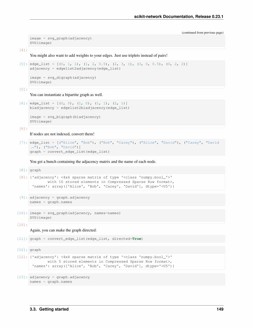
scikit-network Documentation, Release 0.23.1
(continued from previous page)
image = svg_graph(adjacency)SVG(image)
[4]:
You might also want to add weights to your edges. Just use triplets instead of pairs!
[5]: edge_list = [(0, 1, 1), (1, 2, 0.5), (2, 3, 1), (3, 0, 0.5), (0, 2, 2)]adjacency = edgelist2adjacency(edge_list)
image = svg_digraph(adjacency)SVG(image)
[5]:
You can instantiate a bipartite graph as well.
[6]: edge_list = [(0, 0), (1, 0), (1, 1), (2, 1)]biadjacency = edgelist2biadjacency(edge_list)
image = svg_bigraph(biadjacency)SVG(image)
[6]:
If nodes are not indexed, convert them!
[7]: edge_list = [("Alice", "Bob"), ("Bob", "Carey"), ("Alice", "David"), ("Carey", "David→˓"), ("Bob", "David")]graph = convert_edge_list(edge_list)
You get a bunch containing the adjacency matrix and the name of each node.
[8]: graph
[8]: {'adjacency': <4x4 sparse matrix of type '<class 'numpy.bool_'>'with 10 stored elements in Compressed Sparse Row format>,
'names': array(['Alice', 'Bob', 'Carey', 'David'], dtype='<U5')}
[9]: adjacency = graph.adjacencynames = graph.names
[10]: image = svg_graph(adjacency, names=names)SVG(image)
[10]:
Again, you can make the graph directed:
[11]: graph = convert_edge_list(edge_list, directed=True)
[12]: graph
[12]: {'adjacency': <4x4 sparse matrix of type '<class 'numpy.bool_'>'with 5 stored elements in Compressed Sparse Row format>,
'names': array(['Alice', 'Bob', 'Carey', 'David'], dtype='<U5')}
[13]: adjacency = graph.adjacencynames = graph.names
3.3. Getting started 149
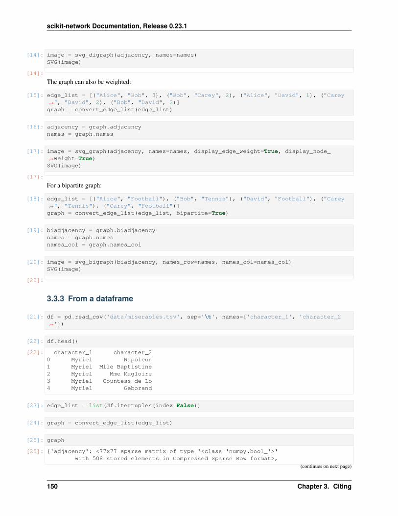
scikit-network Documentation, Release 0.23.1
[14]: image = svg_digraph(adjacency, names=names)SVG(image)
[14]:
The graph can also be weighted:
[15]: edge_list = [("Alice", "Bob", 3), ("Bob", "Carey", 2), ("Alice", "David", 1), ("Carey→˓", "David", 2), ("Bob", "David", 3)]graph = convert_edge_list(edge_list)
[16]: adjacency = graph.adjacencynames = graph.names
[17]: image = svg_graph(adjacency, names=names, display_edge_weight=True, display_node_→˓weight=True)SVG(image)
[17]:
For a bipartite graph:
[18]: edge_list = [("Alice", "Football"), ("Bob", "Tennis"), ("David", "Football"), ("Carey→˓", "Tennis"), ("Carey", "Football")]graph = convert_edge_list(edge_list, bipartite=True)
[19]: biadjacency = graph.biadjacencynames = graph.namesnames_col = graph.names_col
[20]: image = svg_bigraph(biadjacency, names_row=names, names_col=names_col)SVG(image)
[20]:
3.3.3 From a dataframe
[21]: df = pd.read_csv('data/miserables.tsv', sep='\t', names=['character_1', 'character_2→˓'])
[22]: df.head()
[22]: character_1 character_20 Myriel Napoleon1 Myriel Mlle Baptistine2 Myriel Mme Magloire3 Myriel Countess de Lo4 Myriel Geborand
[23]: edge_list = list(df.itertuples(index=False))
[24]: graph = convert_edge_list(edge_list)
[25]: graph
[25]: {'adjacency': <77x77 sparse matrix of type '<class 'numpy.bool_'>'with 508 stored elements in Compressed Sparse Row format>,
(continues on next page)
150 Chapter 3. Citing
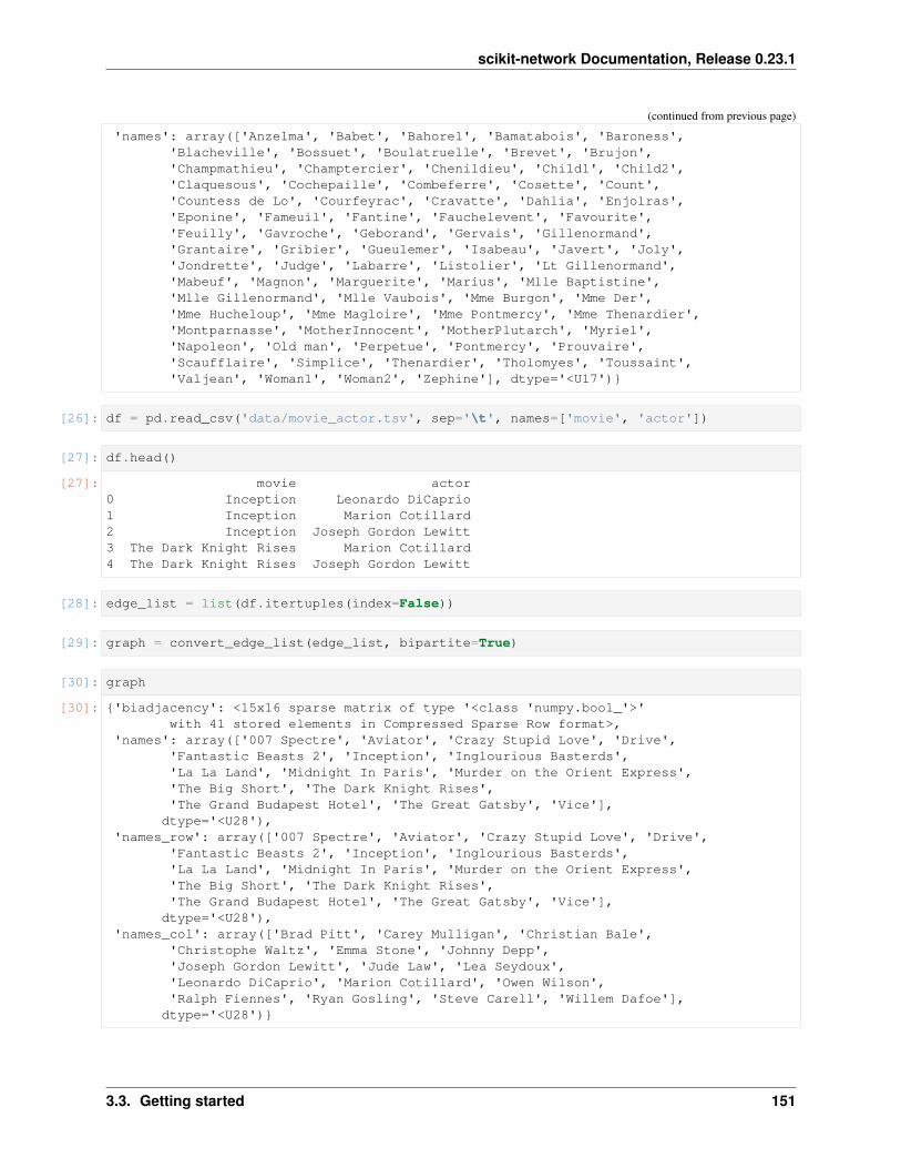
scikit-network Documentation, Release 0.23.1
(continued from previous page)
'names': array(['Anzelma', 'Babet', 'Bahorel', 'Bamatabois', 'Baroness','Blacheville', 'Bossuet', 'Boulatruelle', 'Brevet', 'Brujon','Champmathieu', 'Champtercier', 'Chenildieu', 'Child1', 'Child2','Claquesous', 'Cochepaille', 'Combeferre', 'Cosette', 'Count','Countess de Lo', 'Courfeyrac', 'Cravatte', 'Dahlia', 'Enjolras','Eponine', 'Fameuil', 'Fantine', 'Fauchelevent', 'Favourite','Feuilly', 'Gavroche', 'Geborand', 'Gervais', 'Gillenormand','Grantaire', 'Gribier', 'Gueulemer', 'Isabeau', 'Javert', 'Joly','Jondrette', 'Judge', 'Labarre', 'Listolier', 'Lt Gillenormand','Mabeuf', 'Magnon', 'Marguerite', 'Marius', 'Mlle Baptistine','Mlle Gillenormand', 'Mlle Vaubois', 'Mme Burgon', 'Mme Der','Mme Hucheloup', 'Mme Magloire', 'Mme Pontmercy', 'Mme Thenardier','Montparnasse', 'MotherInnocent', 'MotherPlutarch', 'Myriel','Napoleon', 'Old man', 'Perpetue', 'Pontmercy', 'Prouvaire','Scaufflaire', 'Simplice', 'Thenardier', 'Tholomyes', 'Toussaint','Valjean', 'Woman1', 'Woman2', 'Zephine'], dtype='<U17')}
[26]: df = pd.read_csv('data/movie_actor.tsv', sep='\t', names=['movie', 'actor'])
[27]: df.head()
[27]: movie actor0 Inception Leonardo DiCaprio1 Inception Marion Cotillard2 Inception Joseph Gordon Lewitt3 The Dark Knight Rises Marion Cotillard4 The Dark Knight Rises Joseph Gordon Lewitt
[28]: edge_list = list(df.itertuples(index=False))
[29]: graph = convert_edge_list(edge_list, bipartite=True)
[30]: graph
[30]: {'biadjacency': <15x16 sparse matrix of type '<class 'numpy.bool_'>'with 41 stored elements in Compressed Sparse Row format>,
'names': array(['007 Spectre', 'Aviator', 'Crazy Stupid Love', 'Drive','Fantastic Beasts 2', 'Inception', 'Inglourious Basterds','La La Land', 'Midnight In Paris', 'Murder on the Orient Express','The Big Short', 'The Dark Knight Rises','The Grand Budapest Hotel', 'The Great Gatsby', 'Vice'],
dtype='<U28'),'names_row': array(['007 Spectre', 'Aviator', 'Crazy Stupid Love', 'Drive',
'Fantastic Beasts 2', 'Inception', 'Inglourious Basterds','La La Land', 'Midnight In Paris', 'Murder on the Orient Express','The Big Short', 'The Dark Knight Rises','The Grand Budapest Hotel', 'The Great Gatsby', 'Vice'],
dtype='<U28'),'names_col': array(['Brad Pitt', 'Carey Mulligan', 'Christian Bale',
'Christophe Waltz', 'Emma Stone', 'Johnny Depp','Joseph Gordon Lewitt', 'Jude Law', 'Lea Seydoux','Leonardo DiCaprio', 'Marion Cotillard', 'Owen Wilson','Ralph Fiennes', 'Ryan Gosling', 'Steve Carell', 'Willem Dafoe'],
dtype='<U28')}
3.3. Getting started 151
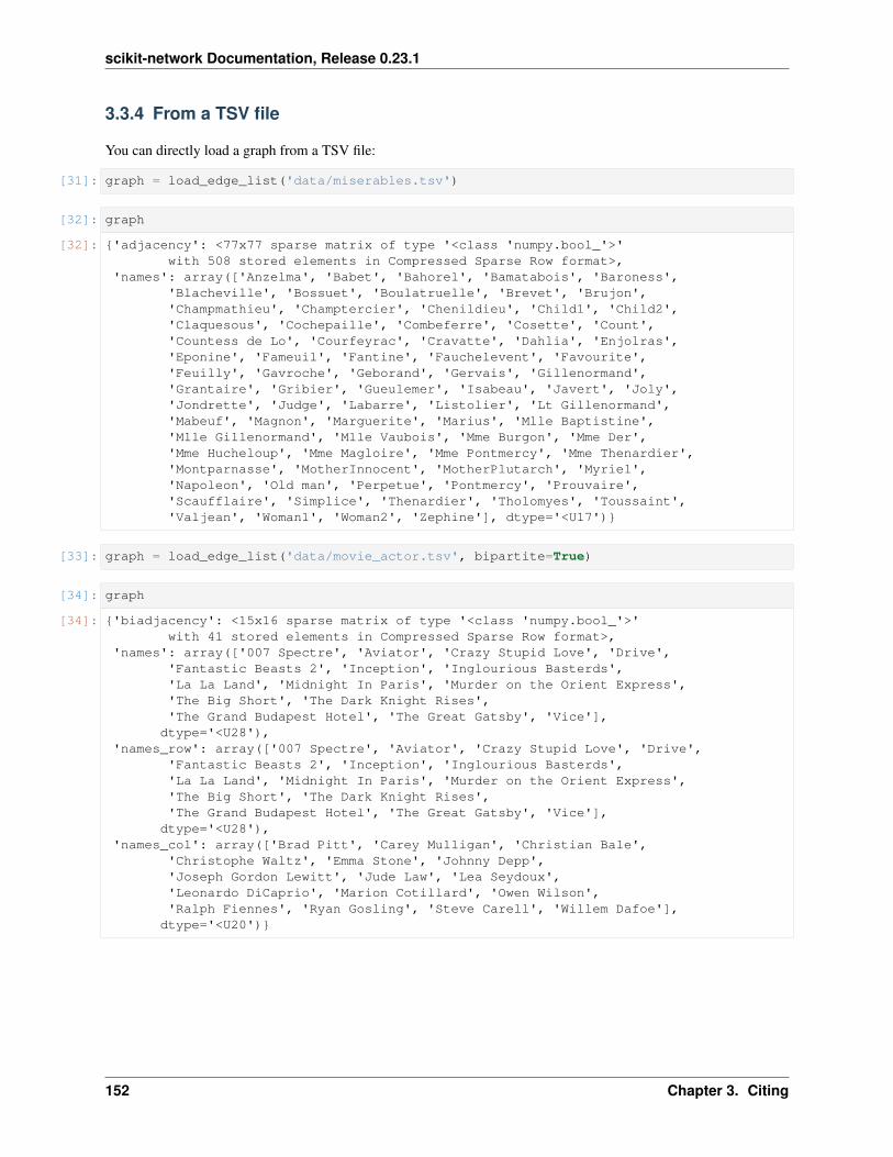
scikit-network Documentation, Release 0.23.1
3.3.4 From a TSV file
You can directly load a graph from a TSV file:
[31]: graph = load_edge_list('data/miserables.tsv')
[32]: graph
[32]: {'adjacency': <77x77 sparse matrix of type '<class 'numpy.bool_'>'with 508 stored elements in Compressed Sparse Row format>,
'names': array(['Anzelma', 'Babet', 'Bahorel', 'Bamatabois', 'Baroness','Blacheville', 'Bossuet', 'Boulatruelle', 'Brevet', 'Brujon','Champmathieu', 'Champtercier', 'Chenildieu', 'Child1', 'Child2','Claquesous', 'Cochepaille', 'Combeferre', 'Cosette', 'Count','Countess de Lo', 'Courfeyrac', 'Cravatte', 'Dahlia', 'Enjolras','Eponine', 'Fameuil', 'Fantine', 'Fauchelevent', 'Favourite','Feuilly', 'Gavroche', 'Geborand', 'Gervais', 'Gillenormand','Grantaire', 'Gribier', 'Gueulemer', 'Isabeau', 'Javert', 'Joly','Jondrette', 'Judge', 'Labarre', 'Listolier', 'Lt Gillenormand','Mabeuf', 'Magnon', 'Marguerite', 'Marius', 'Mlle Baptistine','Mlle Gillenormand', 'Mlle Vaubois', 'Mme Burgon', 'Mme Der','Mme Hucheloup', 'Mme Magloire', 'Mme Pontmercy', 'Mme Thenardier','Montparnasse', 'MotherInnocent', 'MotherPlutarch', 'Myriel','Napoleon', 'Old man', 'Perpetue', 'Pontmercy', 'Prouvaire','Scaufflaire', 'Simplice', 'Thenardier', 'Tholomyes', 'Toussaint','Valjean', 'Woman1', 'Woman2', 'Zephine'], dtype='<U17')}
[33]: graph = load_edge_list('data/movie_actor.tsv', bipartite=True)
[34]: graph
[34]: {'biadjacency': <15x16 sparse matrix of type '<class 'numpy.bool_'>'with 41 stored elements in Compressed Sparse Row format>,
'names': array(['007 Spectre', 'Aviator', 'Crazy Stupid Love', 'Drive','Fantastic Beasts 2', 'Inception', 'Inglourious Basterds','La La Land', 'Midnight In Paris', 'Murder on the Orient Express','The Big Short', 'The Dark Knight Rises','The Grand Budapest Hotel', 'The Great Gatsby', 'Vice'],
dtype='<U28'),'names_row': array(['007 Spectre', 'Aviator', 'Crazy Stupid Love', 'Drive',
'Fantastic Beasts 2', 'Inception', 'Inglourious Basterds','La La Land', 'Midnight In Paris', 'Murder on the Orient Express','The Big Short', 'The Dark Knight Rises','The Grand Budapest Hotel', 'The Great Gatsby', 'Vice'],
dtype='<U28'),'names_col': array(['Brad Pitt', 'Carey Mulligan', 'Christian Bale',
'Christophe Waltz', 'Emma Stone', 'Johnny Depp','Joseph Gordon Lewitt', 'Jude Law', 'Lea Seydoux','Leonardo DiCaprio', 'Marion Cotillard', 'Owen Wilson','Ralph Fiennes', 'Ryan Gosling', 'Steve Carell', 'Willem Dafoe'],
dtype='<U20')}
152 Chapter 3. Citing
scikit-network Documentation, Release 0.23.1
3.3.5 From NetworkX
NetworkX has import and export functions from and towards the CSR format.
3.3.6 Other options
• You have a GraphML file
• You want to test our toy graphs
• You want to generate a graph from a model
• You want to load a graph from one of our referenced repositories (see NetSet and KONECT)
Take a look at the tutorials of the data section!
3.4 Data
3.4.1 Toy graphs
This notebook shows how to load some toy graphs.
[1]: from IPython.display import SVG
[2]: import numpy as np
[3]: from sknetwork.data import house, bow_tie, karate_club, miserables, painters,→˓hourglass, star_wars, movie_actorfrom sknetwork.visualization import svg_graph, svg_digraph, svg_bigraph
Graphs
House graph
[4]: graph = house(metadata=True)adjacency = graph.adjacencyposition = graph.position
[5]: image = svg_graph(adjacency, position, scale=0.5)
[6]: SVG(image)
[6]:
[7]: # adjacency matrix onlyadjacency = house()
Bow tie
[8]: graph = bow_tie(metadata=True)adjacency = graph.adjacencyposition = graph.position
3.4. Data 153
scikit-network Documentation, Release 0.23.1
[9]: image = svg_graph(adjacency, position, scale=0.5)
[10]: SVG(image)
[10]:
Karate club
[11]: graph = karate_club(metadata=True)adjacency = graph.adjacencyposition = graph.positionlabels = graph.labels
[12]: image = svg_graph(adjacency, position, labels=labels)
[13]: SVG(image)
[13]:
Les Miserables
[14]: graph = miserables(metadata=True)adjacency = graph.adjacencyposition = graph.positionnames = graph.names
[15]: image = svg_graph(adjacency, position, names, scale=2)
[16]: SVG(image)
[16]:
Digraphs
[17]: graph = painters(metadata=True)adjacency = graph.adjacencynames = graph.namesposition = graph.position
[18]: image = svg_digraph(adjacency, position, names)
[19]: SVG(image)
[19]:
Bigraphs
Star wars
[20]: graph = star_wars(metadata=True)biadjacency = graph.biadjacencynames_row = graph.names_rownames_col = graph.names_col
[21]: image = svg_bigraph(biadjacency, names_row, names_col)
154 Chapter 3. Citing
scikit-network Documentation, Release 0.23.1
[22]: SVG(image)
[22]:
[23]: # biadjacency matrix onlybiadjacency = star_wars()
Movie-actor
[24]: graph = movie_actor(metadata=True)biadjacency = graph.biadjacencynames_row = graph.names_rownames_col = graph.names_col
[25]: image = svg_bigraph(biadjacency, names_row, names_col)
[26]: SVG(image)
[26]:
3.4.2 Models
This notebook shows how to load some graphs based on simple models.
[1]: from IPython.display import SVG
[2]: import numpy as np
[3]: from sknetwork.data import erdos_renyi, block_model, linear_graph, cyclic_graph,→˓linear_digraph, cyclic_digraph, grid, albert_barabasi, watts_strogatzfrom sknetwork.visualization import svg_graph, svg_digraph
Graphs
Erdos-Renyi model
[4]: adjacency = erdos_renyi(20, 0.2)
[5]: image = svg_graph(adjacency)
[6]: SVG(image)
[6]:
Stochastic block model
[7]: graph = block_model([20,25,30], p_in=[0.5,0.4,0.3], p_out=0.02, metadata=True)adjacency = graph.adjacencylabels = graph.labels
[8]: image = svg_graph(adjacency, labels=labels)
[9]: SVG(image)
3.4. Data 155
scikit-network Documentation, Release 0.23.1
[9]:
Linear graph
[10]: graph = linear_graph(8, metadata=True)adjacency = graph.adjacencyposition = graph.position
[11]: image = svg_graph(adjacency, position)
[12]: SVG(image)
[12]:
[13]: # adjacency matrix onlyadjacency = linear_graph(8)
Cyclic graph
[14]: graph = cyclic_graph(8, metadata=True)adjacency = graph.adjacencyposition = graph.position
[15]: image = svg_graph(adjacency, position, width=200, height=200)
[16]: SVG(image)
[16]:
Grid
[17]: graph = grid(6, 4, metadata=True)adjacency = graph.adjacencyposition = graph.position
[18]: image = svg_graph(adjacency, position)
[19]: SVG(image)
[19]:
Albert-Barabasi model
[20]: adjacency = albert_barabasi(n=100, degree=3)
[21]: image = svg_graph(adjacency, labels={i:0 for i in range(3)}, display_node_weight=True,→˓ node_order=np.flip(np.arange(100)))
[22]: SVG(image)
[22]:
Watts-Strogatz model
[23]: adjacency = watts_strogatz(n=100, degree=6, prob=0.2)
[24]: image = svg_graph(adjacency, display_node_weight=True, node_size_max=10)
[25]: SVG(image)
156 Chapter 3. Citing
scikit-network Documentation, Release 0.23.1
[25]:
Digraphs
Linear graph
[26]: graph = linear_digraph(8, metadata=True)adjacency = graph.adjacencyposition = graph.position
[27]: image = svg_digraph(adjacency, position)
[28]: SVG(image)
[28]:
Cyclic graph
[29]: graph = cyclic_digraph(8, metadata=True)adjacency = graph.adjacencyposition = graph.position
[30]: image = svg_digraph(adjacency, position, width=200, height=200)
[31]: SVG(image)
[31]:
3.4.3 Load
This tutorial shows how to load graphs from files in various formats and from existing collections of datasets, NetSetand Konect.
[1]: from sknetwork.data import load_edge_list, load_graphml, load_netset, load_konect
TSV files
Loading a graph from a TSV file (list of edges).
[2]: graph = load_edge_list('miserables.tsv')adjacency = graph.adjacencynames = graph.names
[3]: # Digraphgraph = load_edge_list('painters.tsv', directed=True)adjacency = graph.adjacencynames = graph.names
[4]: # Bigraphgraph = load_edge_list('movie_actor.tsv', bipartite=True)biadjacency = graph.biadjacencynames_row = graph.names_rownames_col = graph.names_col
3.4. Data 157
scikit-network Documentation, Release 0.23.1
GraphML files
Loading a graph from a GraphML file.
[5]: graph = load_graphml('miserables.graphml')adjacency = graph.adjacencynames = graph.names
[6]: # Digraphgraph = load_graphml('painters.graphml')adjacency = graph.adjacencynames = graph.names
NetSet
Loading a graph from the NetSets collection.
[7]: graph = load_netset('openflights')adjacency = graph.adjacencynames = graph.names
Downloading openflights from NetSet...Unpacking archive...Parsing files...Done.
[8]: # to get all fieldsgraph
[8]: {'adjacency': <3097x3097 sparse matrix of type '<class 'numpy.int64'>'with 36386 stored elements in Compressed Sparse Row format>,
'position': array([[145.39199829, -6.08168983],[145.78900147, -5.20707989],[144.29600525, -5.82678986],...,[131.30599976, -7.98860979],[ 77.81809998, 64.93080139],[ 82.3 , 44.895 ]]),
'meta': {'name': 'openflights','description': 'Airports with daily number of flights between them.','source': 'https://openflights.org'},
'names': array(['Goroka Airport', 'Madang Airport', 'Mount Hagen Kagamuga Airport',..., 'Saumlaki/Olilit Airport', 'Tarko-Sale Airport','Alashankou Bole (Bortala) airport'], dtype='<U65')}
[9]: # Digraphgraph = load_netset('wikivitals')adjacency = graph.adjacencynames = graph.nameslabels = graph.labels
Downloading wikivitals from NetSet...Unpacking archive...Parsing files...Done.
158 Chapter 3. Citing
scikit-network Documentation, Release 0.23.1
[10]: # Bigraphgraph = load_netset('cinema')biadjacency = graph.biadjacency
Downloading cinema from NetSet...Unpacking archive...Parsing files...Done.
Konect
Loading a graph from the Konect collection.
[11]: # first check server availability!# graph = load_konect('dolphins')# adjacency = graph.adjacency
3.4.4 Save
This notebooks shows how to save and load graphs.
[1]: import numpy as npfrom scipy import sparse
[2]: from sknetwork.data import Bunch, load, save
[3]: # random graphadjacency = sparse.csr_matrix(np.random.random((10, 10)) < 0.2)
[4]: # namesnames = list('abcdefghij')
[5]: graph = Bunch()graph.adjacency = adjacencygraph.names = np.array(names)
[6]: save('mygraph', graph)
[7]: graph = load('mygraph')
[8]: graph
[8]: {'adjacency': <10x10 sparse matrix of type '<class 'numpy.bool_'>'with 22 stored elements in Compressed Sparse Row format>,
'names': array(['a', 'b', 'c', 'd', 'e', 'f', 'g', 'h', 'i', 'j'], dtype='<U1')}
3.4. Data 159
scikit-network Documentation, Release 0.23.1
3.5 Topology
3.5.1 Connected components
This notebook illustrates the search for connected components in graphs.
[1]: from IPython.display import SVG
[2]: import numpy as np
[3]: from sknetwork.data import karate_club, painters, movie_actorfrom sknetwork.topology import connected_componentsfrom sknetwork.visualization import svg_graph, svg_digraph, svg_bigraphfrom sknetwork.utils.format import bipartite2undirected
Graphs
[4]: graph = karate_club(metadata=True)adjacency = graph.adjacencyposition = graph.position
[5]: # subgraphk = 15adjacency = adjacency[:k][:,:k]position = position[:k]
[6]: labels = connected_components(adjacency)
[7]: image = svg_graph(adjacency, position, labels=labels)SVG(image)
[7]:
Digraphs
[8]: graph = painters(metadata=True)adjacency = graph.adjacencynames = graph.namesposition = graph.position
[9]: labels = connected_components(adjacency)
[10]: image = svg_digraph(adjacency, position, names, labels)SVG(image)
[10]:
[11]: labels = connected_components(adjacency, connection='strong')
[12]: image = svg_digraph(adjacency, position, names, labels)SVG(image)
160 Chapter 3. Citing
scikit-network Documentation, Release 0.23.1
[12]:
Bigraphs
[13]: graph = movie_actor(metadata=True)biadjacency = graph.biadjacencynames_row = graph.names_rownames_col = graph.names_col
[14]: # subgraphk = 5biadjacency = biadjacency[k:]names_row = names_row[k:]
[15]: adjacency = bipartite2undirected(biadjacency)
[16]: labels = connected_components(adjacency)
[17]: n_row, _ = biadjacency.shapelabels_row = labels[:n_row]labels_col = labels[n_row:]
[18]: image = svg_bigraph(biadjacency, names_row, names_col, labels_row, labels_col)
[19]: SVG(image)
[19]:
3.5.2 Core decomposition
This notebook illustrates the 𝑘-core decomposition of graphs.
[1]: from IPython.display import SVG
[2]: import numpy as np
[3]: from sknetwork.data import karate_club, paintersfrom sknetwork.topology import CoreDecompositionfrom sknetwork.visualization import svg_graph, svg_digraphfrom sknetwork.utils import directed2undirected
Graphs
[4]: graph = karate_club(metadata=True)adjacency = graph.adjacencyposition = graph.position
[5]: core = CoreDecomposition()
3.5. Topology 161
scikit-network Documentation, Release 0.23.1
[6]: labels = core.fit_transform(adjacency)
[7]: image = svg_graph(adjacency, position, scores=labels)SVG(image)
[7]:
Digraphs
[8]: graph = painters(metadata=True)adjacency = graph.adjacencynames = graph.namesposition = graph.position
[9]: labels = core.fit_transform(directed2undirected(adjacency))
[10]: image = svg_digraph(adjacency, position, names, scores=labels)SVG(image)
[10]:
3.5.3 Triangles and cliques
This notebook illustrates clique counting and evaluation of the clustering coefficient of a graph.
[1]: from IPython.display import SVG
[2]: import numpy as np
[3]: from sknetwork.data import karate_clubfrom sknetwork.topology import Triangles, Cliquesfrom sknetwork.visualization import svg_graph
Triangles
[4]: graph = karate_club(metadata=True)adjacency = graph.adjacencyposition = graph.position
[5]: image = svg_graph(adjacency, position)SVG(image)
[5]:
[6]: triangles = Triangles()
[7]: triangles.fit_transform(adjacency)
[7]: 45
[8]: np.round(triangles.clustering_coef_, 2)
[8]: 0.26
162 Chapter 3. Citing
scikit-network Documentation, Release 0.23.1
Cliques
[9]: cliques = Cliques(4)
[10]: cliques.fit_transform(adjacency)
[10]: 11
3.5.4 Graph isomorphism
This notebook illustrates the Weisfeiler-Lehman test of isomorphism.
[1]: from IPython.display import SVGimport numpy as npfrom sknetwork.data import housefrom sknetwork.topology import WeisfeilerLehman, are_isomorphicfrom sknetwork.visualization import svg_graph
Graph labeling
[2]: graph = house(metadata=True)adjacency = graph.adjacencyposition = graph.position
[3]: weisfeiler_lehman = WeisfeilerLehman()labels = weisfeiler_lehman.fit_transform(adjacency)
[4]: image = svg_graph(adjacency, position, labels=labels)SVG(image)
[4]:
[5]: # first iterationweisfeiler_lehman = WeisfeilerLehman(max_iter=1)labels = weisfeiler_lehman.fit_transform(adjacency)
[6]: image = svg_graph(adjacency, position, labels=labels)SVG(image)
[6]:
Weisfeiler-Lehman test
[7]: adjacency_1 = house()
n = adjacency_1.indptr.shape[0] - 1reorder = list(range(n))np.random.shuffle(reorder)adjacency_2 = adjacency_1[reorder][:, reorder]
are_isomorphic(adjacency_1, adjacency_2)
[7]: True
3.5. Topology 163
scikit-network Documentation, Release 0.23.1
3.6 Path
3.6.1 Distance
This notebook illustrates the computation of distances between nodes in graphs (in number of hops).
[1]: from IPython.display import SVG
[2]: import numpy as np
[3]: from sknetwork.data import miserables, painters, movie_actorfrom sknetwork.path import distancefrom sknetwork.visualization import svg_graph, svg_digraph, svg_bigraphfrom sknetwork.utils import bipartite2undirected
Graphs
[4]: graph = miserables(metadata=True)adjacency = graph.adjacencynames = graph.namesposition = graph.position
[5]: napoleon = 1
[6]: dist = distance(adjacency, sources=napoleon)
[7]: image = svg_graph(adjacency, position, names, scores = -dist, seeds=[napoleon], scale→˓= 1.5)
[8]: SVG(image)
[8]:
Digraphs
[9]: graph = painters(metadata=True)adjacency = graph.adjacencynames = graph.namesposition = graph.position
[10]: cezanne = 11
[11]: dist = distance(adjacency, sources=cezanne)
[12]: dist_neg= {i: -d for i, d in enumerate(dist) if d < np.inf}
[13]: image = svg_digraph(adjacency, position, names, scores=dist_neg , seeds=[cezanne])
[14]: SVG(image)
164 Chapter 3. Citing
scikit-network Documentation, Release 0.23.1
[14]:
Bigraphs
[15]: graph = movie_actor(metadata=True)biadjacency = graph.biadjacencynames_row = graph.names_rownames_col = graph.names_col
[16]: adjacency = bipartite2undirected(biadjacency)
[17]: n_row, _ = biadjacency.shape
[18]: seydoux = 9
[19]: dist = distance(adjacency, sources=seydoux + n_row)
[20]: image = svg_bigraph(biadjacency, names_row, names_col, scores_col=-dist[n_row:],→˓seeds_col=seydoux)
[21]: SVG(image)
[21]:
3.6.2 Shortest paths
This notebook illustrates the search for shortest paths in graphs.
[1]: from IPython.display import SVG
[2]: import numpy as np
[3]: from sknetwork.data import miserables, painters, movie_actorfrom sknetwork.path import shortest_pathfrom sknetwork.visualization import svg_graph, svg_digraph, svg_bigraphfrom sknetwork.utils import bipartite2undirected
Graphs
[4]: graph = miserables(metadata=True)adjacency = graph.adjacencynames = graph.namesposition = graph.position
[5]: napoleon = 1jondrette = 46
[6]: path = shortest_path(adjacency, sources=napoleon, targets=jondrette)
3.6. Path 165
scikit-network Documentation, Release 0.23.1
[7]: edge_labels = [(path[k], path[k + 1], 0) for k in range(len(path) - 1)]
[8]: image = svg_graph(adjacency, position, names, edge_labels=edge_labels, edge_width=3,→˓display_edge_weight=False, scale = 1.5)
[9]: SVG(image)
[9]:
Digraphs
[10]: graph = painters(metadata=True)adjacency = graph.adjacencynames = graph.namesposition = graph.position
[11]: klimt = 6vinci = 9
[12]: path = shortest_path(adjacency, sources=klimt, targets=vinci)
[13]: edge_labels = [(path[k], path[k + 1], 0) for k in range(len(path) - 1)]
[14]: image = svg_digraph(adjacency, position, names, edge_labels=edge_labels, edge_width=2)
[15]: SVG(image)
[15]:
Bigraphs
[16]: graph = movie_actor(metadata=True)biadjacency = graph.biadjacencynames_row = graph.names_rownames_col = graph.names_col
[17]: adjacency = bipartite2undirected(biadjacency)
[18]: n_row, _ = biadjacency.shape
[19]: seydoux = 9lewitt = 2
[20]: path = shortest_path(adjacency, sources=seydoux + n_row, targets=lewitt + n_row)
[21]: edge_labels = []labels_row = {}labels_col = {}for k in range(len(path) - 1):
i = path[k]j = path[k + 1]
(continues on next page)
166 Chapter 3. Citing
scikit-network Documentation, Release 0.23.1
(continued from previous page)
# row firstif i > j:
i, j = j, ij -= n_rowlabels_row[i] = 0labels_col[j] = 0edge_labels.append((i, j, 0))
[22]: image = svg_bigraph(biadjacency, names_row, names_col, labels_row, labels_col,edge_labels=edge_labels, edge_color='gray', edge_width=3)
[23]: SVG(image)
[23]:
3.7 Clustering
3.7.1 Louvain
This notebook illustrates the clustering of a graph by the Louvain algorithm.
[1]: from IPython.display import SVG
[2]: import numpy as np
[3]: from sknetwork.data import karate_club, painters, movie_actorfrom sknetwork.clustering import Louvain, BiLouvain, modularity, bimodularityfrom sknetwork.linalg import normalizefrom sknetwork.utils import bipartite2undirected, membership_matrixfrom sknetwork.visualization import svg_graph, svg_digraph, svg_bigraph
Graphs
[4]: graph = karate_club(metadata=True)adjacency = graph.adjacencyposition = graph.position
Clustering
[5]: louvain = Louvain()labels = louvain.fit_transform(adjacency)
[6]: labels_unique, counts = np.unique(labels, return_counts=True)print(labels_unique, counts)
[0 1 2 3] [12 11 6 5]
[7]: image = svg_graph(adjacency, position, labels=labels)
[8]: SVG(image)
3.7. Clustering 167
scikit-network Documentation, Release 0.23.1
[8]:
Metrics
[9]: modularity(adjacency, labels)
[9]: 0.4188034188034188
Aggregate graph
[10]: adjacency_aggregate = louvain.adjacency_
[11]: average = normalize(membership_matrix(labels).T)position_aggregate = average.dot(position)labels_unique, counts = np.unique(labels, return_counts=True)
[12]: image = svg_graph(adjacency_aggregate, position_aggregate, counts, labels=labels_→˓unique,
display_node_weight=True, node_weights=counts)
[13]: SVG(image)
[13]:
Soft clustering
[14]: scores = louvain.membership_[:,1].toarray().ravel()
[15]: image = svg_graph(adjacency, position, scores=scores)
[16]: SVG(image)
[16]:
Digraphs
[17]: graph = painters(metadata=True)adjacency = graph.adjacencynames = graph.namesposition = graph.position
Clustering
[18]: louvain = Louvain()labels = louvain.fit_transform(adjacency)
[19]: labels_unique, counts = np.unique(labels, return_counts=True)print(labels_unique, counts)
[0 1 2] [5 5 4]
[20]: image = svg_digraph(adjacency, position, names, labels)
[21]: SVG(image)
[21]:
Metrics
168 Chapter 3. Citing
scikit-network Documentation, Release 0.23.1
[22]: modularity(adjacency, labels)
[22]: 0.32480000000000003
Aggregate graph
[23]: adjacency_aggregate = louvain.adjacency_
[24]: average = normalize(membership_matrix(labels).T)position_aggregate = average.dot(position)labels_unique, counts = np.unique(labels, return_counts=True)
[25]: image = svg_digraph(adjacency_aggregate, position_aggregate, counts, labels=labels_→˓unique,
display_node_weight=True, node_weights=counts)
[26]: SVG(image)
[26]:
Soft clustering
[27]: scores = louvain.membership_[:,1].toarray().ravel()
[28]: image = svg_graph(adjacency, position, scores=scores)
[29]: SVG(image)
[29]:
Bigraphs
[30]: graph = movie_actor(metadata=True)biadjacency = graph.biadjacencynames_row = graph.names_rownames_col = graph.names_col
Clustering by BiLouvain
[31]: bilouvain = BiLouvain()bilouvain.fit(biadjacency)labels_row = bilouvain.labels_row_labels_col = bilouvain.labels_col_
[32]: image = svg_bigraph(biadjacency, names_row, names_col, labels_row, labels_col)
[33]: SVG(image)
[33]:
Metrics
[34]: bimodularity(biadjacency, labels_row, labels_col)
[34]: 0.5742630385487529
Aggregate graph
3.7. Clustering 169
scikit-network Documentation, Release 0.23.1
[35]: biadjacency_aggregate = bilouvain.biadjacency_
[36]: labels_unique_row, counts_row = np.unique(labels_row, return_counts=True)labels_unique_col, counts_col = np.unique(labels_col, return_counts=True)
[37]: image = svg_bigraph(biadjacency_aggregate, counts_row, counts_col, labels_unique_row,→˓labels_unique_col,
display_node_weight=True, node_weights_row=counts_row, node_→˓weights_col=counts_col,
scale=0.5)
[38]: SVG(image)
[38]:
Soft clustering
[39]: scores_row = bilouvain.membership_row_[:,1].toarray().ravel()scores_col = bilouvain.membership_col_[:,1].toarray().ravel()
[40]: image = svg_bigraph(biadjacency, names_row, names_col, scores_row=scores_row, scores_→˓col=scores_col)
[41]: SVG(image)
[41]:
Clustering by Louvain
[42]: louvain = Louvain()adjacency = bipartite2undirected(biadjacency)labels = louvain.fit_transform(adjacency)
[43]: n_row = biadjacency.shape[0]labels_row = louvain.labels_[:n_row]labels_col = louvain.labels_[n_row:]
[44]: image = svg_bigraph(biadjacency, names_row, names_col, labels_row, labels_col)
[45]: SVG(image)
[45]:
Aggregate graph
[46]: biadjacency_aggregate = louvain.adjacency_[:n_row][:n_row]
[47]: labels_unique_row, counts_row = np.unique(labels_row, return_counts=True)labels_unique_col, counts_col = np.unique(labels_col, return_counts=True)
[48]: image = svg_bigraph(biadjacency_aggregate, counts_row, counts_col, labels_unique_row,→˓labels_unique_col,
display_node_weight=True, node_weights_row=counts_row, node_→˓weights_col=counts_col)
[49]: SVG(image)
170 Chapter 3. Citing
scikit-network Documentation, Release 0.23.1
[49]:
3.7.2 Propagation
This notebook illustrates the clustering of a graph by label propagation.
[1]: from IPython.display import SVG
[2]: import numpy as np
[3]: from sknetwork.data import karate_club, painters, movie_actorfrom sknetwork.clustering import PropagationClustering, BiPropagationClustering,→˓modularity, bimodularityfrom sknetwork.linalg import normalizefrom sknetwork.utils import bipartite2undirected, membership_matrixfrom sknetwork.visualization import svg_graph, svg_digraph, svg_bigraph
Graphs
[4]: graph = karate_club(metadata=True)adjacency = graph.adjacencyposition = graph.position
Clustering
[5]: propagation = PropagationClustering()labels = propagation.fit_transform(adjacency)
[6]: labels_unique, counts = np.unique(labels, return_counts=True)print(labels_unique, counts)
[0 1] [19 15]
[7]: image = svg_graph(adjacency, position, labels=labels)
[8]: SVG(image)
[8]:
Metrics
[9]: modularity(adjacency, labels)
[9]: 0.35231755424063116
Aggregate graph
[10]: adjacency_aggregate = propagation.adjacency_
[11]: average = normalize(membership_matrix(labels).T)position_aggregate = average.dot(position)labels_unique, counts = np.unique(labels, return_counts=True)
3.7. Clustering 171
scikit-network Documentation, Release 0.23.1
[12]: image = svg_graph(adjacency_aggregate, position_aggregate, counts, labels=labels_→˓unique,
display_node_weight=True, node_weights=counts)
[13]: SVG(image)
[13]:
Soft clustering
[14]: scores = propagation.membership_[:,1].toarray().ravel()
[15]: image = svg_graph(adjacency, position, scores=scores)
[16]: SVG(image)
[16]:
Digraphs
[17]: graph = painters(metadata=True)adjacency = graph.adjacencynames = graph.namesposition = graph.position
Clustering
[18]: propagation = PropagationClustering()labels = propagation.fit_transform(adjacency)
[19]: labels_unique, counts = np.unique(labels, return_counts=True)print(labels_unique, counts)
[0 1] [10 4]
[20]: image = svg_digraph(adjacency, position, names, labels)
[21]: SVG(image)
[21]:
Metrics
[22]: modularity(adjacency, labels)
[22]: 0.256
Aggregate graph
[23]: adjacency_aggregate = propagation.adjacency_
[24]: average = normalize(membership_matrix(labels).T)position_aggregate = average.dot(position)labels_unique, counts = np.unique(labels, return_counts=True)
[25]: image = svg_digraph(adjacency_aggregate, position_aggregate, counts, labels=labels_→˓unique,
display_node_weight=True, node_weights=counts)
172 Chapter 3. Citing
scikit-network Documentation, Release 0.23.1
[26]: SVG(image)
[26]:
Soft clustering
[27]: scores = propagation.membership_[:,0].toarray().ravel()
[28]: image = svg_graph(adjacency, position, scores=scores)
[29]: SVG(image)
[29]:
Bigraphs
[30]: graph = movie_actor(metadata=True)biadjacency = graph.biadjacencynames_row = graph.names_rownames_col = graph.names_col
Clustering
[31]: bipropagation = BiPropagationClustering()bipropagation.fit(biadjacency)labels_row = bipropagation.labels_row_labels_col = bipropagation.labels_col_
[32]: image = svg_bigraph(biadjacency, names_row, names_col, labels_row, labels_col)
[33]: SVG(image)
[33]:
Metrics
[34]: bimodularity(biadjacency, labels_row, labels_col)
[34]: 0.41496598639455773
Aggregate graph
[35]: biadjacency_aggregate = bipropagation.biadjacency_
[36]: labels_unique_row, counts_row = np.unique(labels_row, return_counts=True)labels_unique_col, counts_col = np.unique(labels_col, return_counts=True)
[37]: image = svg_bigraph(biadjacency_aggregate, counts_row, counts_col, labels_unique_row,→˓labels_unique_col,
display_node_weight=True, node_weights_row=counts_row, node_→˓weights_col=counts_col)
[38]: SVG(image)
[38]:
Soft clustering
3.7. Clustering 173
scikit-network Documentation, Release 0.23.1
[39]: scores_row = bipropagation.membership_row_[:,1].toarray().ravel()scores_col = bipropagation.membership_col_[:,1].toarray().ravel()
[40]: image = svg_bigraph(biadjacency, names_row, names_col, scores_row=scores_row, scores_→˓col=scores_col)
[41]: SVG(image)
[41]:
3.7.3 K-means
This notebook illustrates the clustering of a graph by k-means. This clustering involves the embedding of the graph ina space of low dimension.
[1]: from IPython.display import SVG
[2]: import numpy as np
[3]: from sknetwork.data import karate_club, painters, movie_actorfrom sknetwork.clustering import KMeans, BiKMeans, modularity, bimodularityfrom sknetwork.linalg import normalizefrom sknetwork.embedding import GSVDfrom sknetwork.utils import membership_matrixfrom sknetwork.visualization import svg_graph, svg_digraph, svg_bigraph
Graphs
[4]: graph = karate_club(metadata=True)adjacency = graph.adjacencyposition = graph.position
Clustering
[5]: kmeans = KMeans(n_clusters = 2, embedding_method=GSVD(3))labels = kmeans.fit_transform(adjacency)
[6]: unique_labels, counts = np.unique(labels, return_counts=True)print(unique_labels, counts)
[0 1] [19 15]
[7]: image = svg_graph(adjacency, position, labels=labels)
[8]: SVG(image)
[8]:
Metrics
[9]: modularity(adjacency, labels)
[9]: 0.3599605522682445
Aggregate graph
174 Chapter 3. Citing
scikit-network Documentation, Release 0.23.1
[10]: adjacency_aggregate = kmeans.adjacency_
[11]: average = normalize(membership_matrix(labels).T)position_aggregate = average.dot(position)labels_unique, counts = np.unique(labels, return_counts=True)
[12]: image = svg_graph(adjacency_aggregate, position_aggregate, counts, labels=labels_→˓unique,
display_node_weight=True, node_weights=counts)
[13]: SVG(image)
[13]:
Soft clustering
[14]: scores = kmeans.membership_[:,1].toarray().ravel()
[15]: image = svg_graph(adjacency, position, scores=scores)
[16]: SVG(image)
[16]:
Digraphs
[17]: graph = painters(metadata=True)adjacency = graph.adjacencyposition = graph.positionnames = graph.names
Clustering
[18]: kmeans = KMeans(3, GSVD(3))labels = kmeans.fit_transform(adjacency)
[19]: image = svg_digraph(adjacency, position, names=names, labels=labels)
[20]: SVG(image)
[20]:
Metrics
[21]: modularity(adjacency, labels)
[21]: 0.23999999999999988
Aggregate graph
[22]: adjacency_aggregate = kmeans.adjacency_
[23]: average = normalize(membership_matrix(labels).T)position_aggregate = average.dot(position)labels_unique, counts = np.unique(labels, return_counts=True)
3.7. Clustering 175
scikit-network Documentation, Release 0.23.1
[24]: image = svg_digraph(adjacency_aggregate, position_aggregate, counts, labels=labels_→˓unique,
display_node_weight=True, node_weights=counts)
[25]: SVG(image)
[25]:
Soft clustering
[26]: scores = kmeans.membership_[:,1].toarray().ravel()
[27]: image = svg_digraph(adjacency, position, scores=scores)
[28]: SVG(image)
[28]:
Bigraphs
[29]: graph = movie_actor(metadata=True)biadjacency = graph.biadjacencynames_row = graph.names_rownames_col = graph.names_col
Clustering
[30]: bikmeans = BiKMeans(3, GSVD(3), co_cluster=True)bikmeans.fit(biadjacency)labels_row = bikmeans.labels_row_labels_col = bikmeans.labels_col_
[31]: image = svg_bigraph(biadjacency, names_row, names_col, labels_row, labels_col)
[32]: SVG(image)
[32]:
Metrics
[33]: bimodularity(biadjacency, labels_row, labels_col)
[33]: 0.4943310657596373
Aggregate graph
[34]: biadjacency_aggregate = bikmeans.biadjacency_
[35]: labels_unique_row, counts_row = np.unique(labels_row, return_counts=True)labels_unique_col, counts_col = np.unique(labels_col, return_counts=True)
[36]: image = svg_bigraph(biadjacency_aggregate, counts_row, counts_col, labels_unique_row,→˓labels_unique_col,
display_node_weight=True, node_weights_row=counts_row, node_→˓weights_col=counts_col)
176 Chapter 3. Citing
scikit-network Documentation, Release 0.23.1
[37]: SVG(image)
[37]:
Soft clustering
[38]: scores_row = bikmeans.membership_row_[:,1].toarray().ravel()scores_col = bikmeans.membership_col_[:,1].toarray().ravel()
[39]: image = svg_bigraph(biadjacency, names_row, names_col, scores_row=scores_row, scores_→˓col=scores_col)
[40]: SVG(image)
[40]:
3.8 Hierarchy
3.8.1 Paris
This notebook illustrates the hierarchical clustering of graphs by the Paris algorithm.
[1]: from IPython.display import SVG
[2]: import numpy as np
[3]: from sknetwork.data import karate_club, painters, movie_actorfrom sknetwork.hierarchy import Paris, BiParis, cut_straight, dasgupta_score, tree_→˓sampling_divergencefrom sknetwork.visualization import svg_graph, svg_digraph, svg_bigraph, svg_→˓dendrogram
Graphs
[4]: graph = karate_club(metadata=True)adjacency = graph.adjacencyposition = graph.position
Hierarchy
[5]: paris = Paris()dendrogram = paris.fit_transform(adjacency)
[6]: image = svg_dendrogram(dendrogram)
[7]: SVG(image)
[7]:
Cuts of the dendrogram
[8]: labels = cut_straight(dendrogram)print(labels)
3.8. Hierarchy 177
scikit-network Documentation, Release 0.23.1
[1 1 1 1 1 1 1 1 0 1 1 1 1 1 0 0 1 1 0 1 0 1 0 0 0 0 0 0 0 0 0 0 0 0]
[9]: n_clusters = 4labels, dendrogram_aggregate = cut_straight(dendrogram, n_clusters, return_→˓dendrogram=True)print(labels)
[0 0 0 0 3 3 3 0 1 0 3 0 0 0 1 1 3 0 1 0 1 0 1 2 2 2 2 2 2 2 1 2 1 1]
[10]: _, counts = np.unique(labels, return_counts=True)
[11]: image = svg_dendrogram(dendrogram_aggregate, names=counts, rotate_names=False)
[12]: SVG(image)
[12]:
[13]: image = svg_graph(adjacency, position, labels=labels)
[14]: SVG(image)
[14]:
Metrics
[15]: dasgupta_score(adjacency, dendrogram)
[15]: 0.6655354449472097
[16]: tree_sampling_divergence(adjacency, dendrogram)
[16]: 0.4867262842323475
Digraphs
[17]: graph = painters(metadata=True)adjacency = graph.adjacencyposition = graph.positionnames = graph.names
Hierarchy
[18]: paris = Paris()dendrogram = paris.fit_transform(adjacency)
[19]: image = svg_dendrogram(dendrogram, names, n_clusters=3, rotate=True)
[20]: SVG(image)
[20]:
Cuts of the dendrogram
[21]: # cut with 3 clusterslabels = cut_straight(dendrogram, n_clusters = 3)print(labels)
178 Chapter 3. Citing
scikit-network Documentation, Release 0.23.1
[0 0 1 0 1 1 2 0 0 1 0 0 0 2]
[22]: image = svg_digraph(adjacency, position, names=names, labels=labels)
[23]: SVG(image)
[23]:
Metrics
[24]: dasgupta_score(adjacency, dendrogram)
[24]: 0.5842857142857143
[25]: tree_sampling_divergence(adjacency, dendrogram)
[25]: 0.4685697020629489
Bigraphs
[26]: graph = movie_actor(metadata=True)biadjacency = graph.biadjacencynames_row = graph.names_rownames_col = graph.names_col
Hierarchy
[27]: biparis = BiParis()biparis.fit(biadjacency)dendrogram_row = biparis.dendrogram_row_dendrogram_col = biparis.dendrogram_col_dendrogram_full = biparis.dendrogram_full_
[28]: image = svg_dendrogram(dendrogram_row, names_row, n_clusters=4, rotate=True)
[29]: SVG(image)
[29]:
[30]: image = svg_dendrogram(dendrogram_col, names_col, n_clusters=4, rotate=True)
[31]: SVG(image)
[31]:
Cuts of the dendrogram
[32]: labels = cut_straight(dendrogram_full, n_clusters = 4)n_row = biadjacency.shape[0]labels_row = labels[:n_row]labels_col = labels[n_row:]
[33]: image = svg_bigraph(biadjacency, names_row, names_col, labels_row, labels_col)
[34]: SVG(image)
[34]:
3.8. Hierarchy 179
scikit-network Documentation, Release 0.23.1
3.8.2 Ward
This notebook illustrates the hierarchical clustering of graphs by the Ward method, after embedding in a space of lowdimension.
[1]: from IPython.display import SVG
[2]: import numpy as np
[3]: from sknetwork.data import karate_club, painters, movie_actorfrom sknetwork.embedding import Spectralfrom sknetwork.hierarchy import Ward, BiWard, cut_straight, dasgupta_score, tree_→˓sampling_divergencefrom sknetwork.visualization import svg_graph, svg_digraph, svg_bigraph, svg_→˓dendrogram
Graphs
[4]: graph = karate_club(metadata=True)adjacency = graph.adjacencyposition = graph.position
Hierarchy
[5]: ward = Ward()dendrogram = ward.fit_transform(adjacency)
[6]: image = svg_dendrogram(dendrogram)
[7]: SVG(image)
[7]:
Cuts of the dendrogram
[8]: labels = cut_straight(dendrogram)print(labels)
[1 1 1 1 1 1 1 1 0 0 1 1 1 1 0 0 1 1 0 1 0 1 0 0 0 0 0 0 0 0 0 0 0 0]
[9]: n_clusters = 4labels, dendrogram_aggregate = cut_straight(dendrogram, n_clusters, return_→˓dendrogram=True)print(labels)
[1 1 1 1 3 3 3 1 0 0 3 1 1 1 2 2 3 1 2 1 2 1 2 0 0 0 0 0 0 2 2 0 0 0]
[10]: _, counts = np.unique(labels, return_counts=True)
[11]: image = svg_dendrogram(dendrogram_aggregate, names=counts, rotate_names=False)
[12]: SVG(image)
[12]:
180 Chapter 3. Citing
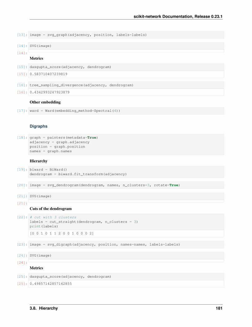
scikit-network Documentation, Release 0.23.1
[13]: image = svg_graph(adjacency, position, labels=labels)
[14]: SVG(image)
[14]:
Metrics
[15]: dasgupta_score(adjacency, dendrogram)
[15]: 0.583710407239819
[16]: tree_sampling_divergence(adjacency, dendrogram)
[16]: 0.4342993247923879
Other embedding
[17]: ward = Ward(embedding_method=Spectral(4))
Digraphs
[18]: graph = painters(metadata=True)adjacency = graph.adjacencyposition = graph.positionnames = graph.names
Hierarchy
[19]: biward = BiWard()dendrogram = biward.fit_transform(adjacency)
[20]: image = svg_dendrogram(dendrogram, names, n_clusters=3, rotate=True)
[21]: SVG(image)
[21]:
Cuts of the dendrogram
[22]: # cut with 3 clusterslabels = cut_straight(dendrogram, n_clusters = 3)print(labels)
[0 0 1 0 1 1 2 0 0 1 0 0 0 2]
[23]: image = svg_digraph(adjacency, position, names=names, labels=labels)
[24]: SVG(image)
[24]:
Metrics
[25]: dasgupta_score(adjacency, dendrogram)
[25]: 0.49857142857142855
3.8. Hierarchy 181
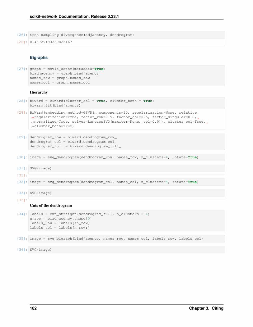
scikit-network Documentation, Release 0.23.1
[26]: tree_sampling_divergence(adjacency, dendrogram)
[26]: 0.48729193280825467
Bigraphs
[27]: graph = movie_actor(metadata=True)biadjacency = graph.biadjacencynames_row = graph.names_rownames_col = graph.names_col
Hierarchy
[28]: biward = BiWard(cluster_col = True, cluster_both = True)biward.fit(biadjacency)
[28]: BiWard(embedding_method=GSVD(n_components=10, regularization=None, relative_→˓regularization=True, factor_row=0.5, factor_col=0.5, factor_singular=0.0,→˓normalized=True, solver=LanczosSVD(maxiter=None, tol=0.0)), cluster_col=True,→˓cluster_both=True)
[29]: dendrogram_row = biward.dendrogram_row_dendrogram_col = biward.dendrogram_col_dendrogram_full = biward.dendrogram_full_
[30]: image = svg_dendrogram(dendrogram_row, names_row, n_clusters=4, rotate=True)
[31]: SVG(image)
[31]:
[32]: image = svg_dendrogram(dendrogram_col, names_col, n_clusters=4, rotate=True)
[33]: SVG(image)
[33]:
Cuts of the dendrogram
[34]: labels = cut_straight(dendrogram_full, n_clusters = 4)n_row = biadjacency.shape[0]labels_row = labels[:n_row]labels_col = labels[n_row:]
[35]: image = svg_bigraph(biadjacency, names_row, names_col, labels_row, labels_col)
[36]: SVG(image)
182 Chapter 3. Citing
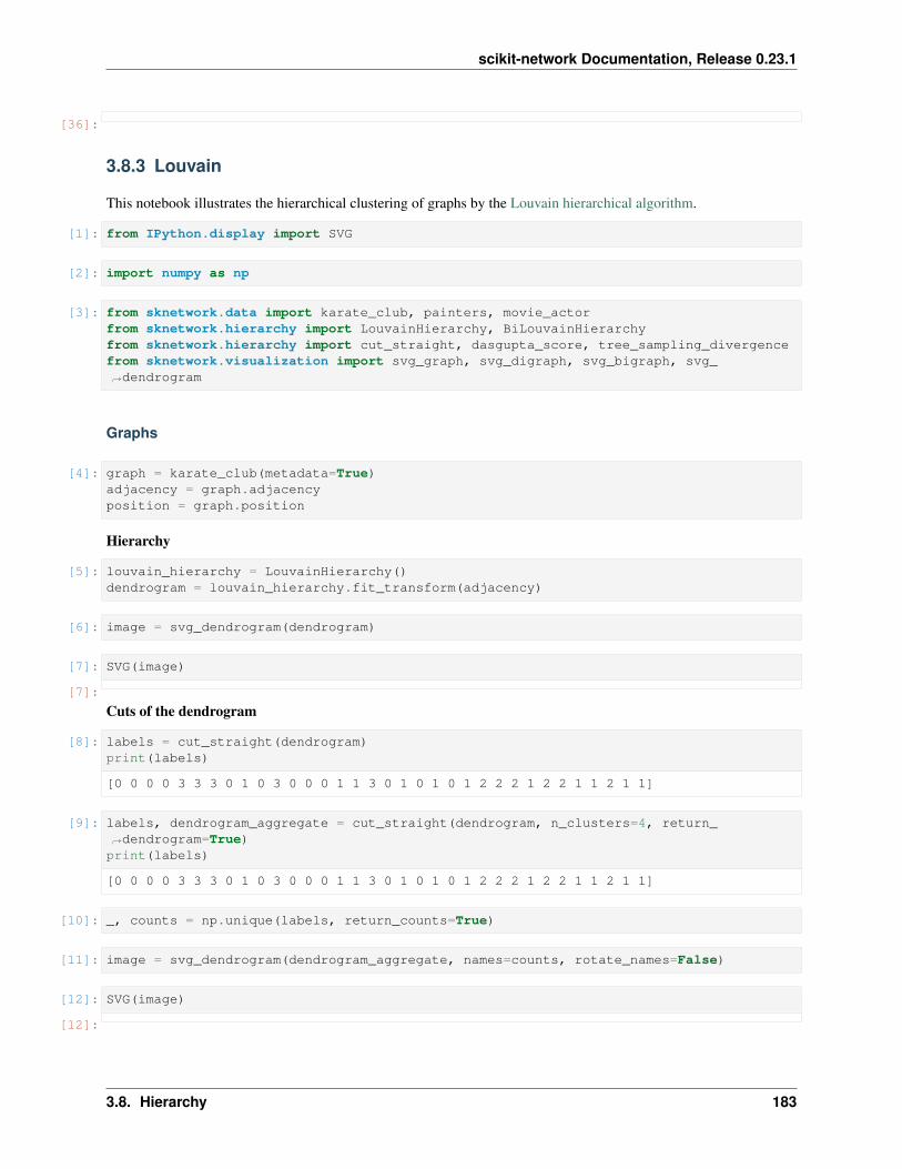
scikit-network Documentation, Release 0.23.1
[36]:
3.8.3 Louvain
This notebook illustrates the hierarchical clustering of graphs by the Louvain hierarchical algorithm.
[1]: from IPython.display import SVG
[2]: import numpy as np
[3]: from sknetwork.data import karate_club, painters, movie_actorfrom sknetwork.hierarchy import LouvainHierarchy, BiLouvainHierarchyfrom sknetwork.hierarchy import cut_straight, dasgupta_score, tree_sampling_divergencefrom sknetwork.visualization import svg_graph, svg_digraph, svg_bigraph, svg_→˓dendrogram
Graphs
[4]: graph = karate_club(metadata=True)adjacency = graph.adjacencyposition = graph.position
Hierarchy
[5]: louvain_hierarchy = LouvainHierarchy()dendrogram = louvain_hierarchy.fit_transform(adjacency)
[6]: image = svg_dendrogram(dendrogram)
[7]: SVG(image)
[7]:
Cuts of the dendrogram
[8]: labels = cut_straight(dendrogram)print(labels)
[0 0 0 0 3 3 3 0 1 0 3 0 0 0 1 1 3 0 1 0 1 0 1 2 2 2 1 2 2 1 1 2 1 1]
[9]: labels, dendrogram_aggregate = cut_straight(dendrogram, n_clusters=4, return_→˓dendrogram=True)print(labels)
[0 0 0 0 3 3 3 0 1 0 3 0 0 0 1 1 3 0 1 0 1 0 1 2 2 2 1 2 2 1 1 2 1 1]
[10]: _, counts = np.unique(labels, return_counts=True)
[11]: image = svg_dendrogram(dendrogram_aggregate, names=counts, rotate_names=False)
[12]: SVG(image)
[12]:
3.8. Hierarchy 183
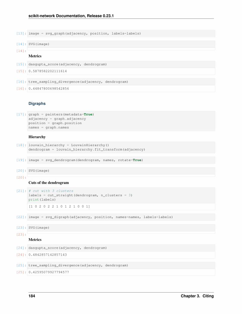
scikit-network Documentation, Release 0.23.1
[13]: image = svg_graph(adjacency, position, labels=labels)
[14]: SVG(image)
[14]:
Metrics
[15]: dasgupta_score(adjacency, dendrogram)
[15]: 0.5878582202111614
[16]: tree_sampling_divergence(adjacency, dendrogram)
[16]: 0.44847800698542856
Digraphs
[17]: graph = painters(metadata=True)adjacency = graph.adjacencyposition = graph.positionnames = graph.names
Hierarchy
[18]: louvain_hierarchy = LouvainHierarchy()dendrogram = louvain_hierarchy.fit_transform(adjacency)
[19]: image = svg_dendrogram(dendrogram, names, rotate=True)
[20]: SVG(image)
[20]:
Cuts of the dendrogram
[21]: # cut with 3 clusterslabels = cut_straight(dendrogram, n_clusters = 3)print(labels)
[1 0 2 0 2 2 1 0 1 2 1 0 0 1]
[22]: image = svg_digraph(adjacency, position, names=names, labels=labels)
[23]: SVG(image)
[23]:
Metrics
[24]: dasgupta_score(adjacency, dendrogram)
[24]: 0.4842857142857143
[25]: tree_sampling_divergence(adjacency, dendrogram)
[25]: 0.42595079927794577
184 Chapter 3. Citing
scikit-network Documentation, Release 0.23.1
Bigraphs
[26]: graph = movie_actor(metadata=True)biadjacency = graph.biadjacencynames_row = graph.names_rownames_col = graph.names_col
Hierarchy
[27]: bilouvain = BiLouvainHierarchy()bilouvain.fit(biadjacency)dendrogram_row = bilouvain.dendrogram_row_dendrogram_col = bilouvain.dendrogram_col_dendrogram_full = bilouvain.dendrogram_full_
[28]: image = svg_dendrogram(dendrogram_row, names_row, n_clusters=4, rotate=True)
[29]: SVG(image)
[29]:
[30]: image = svg_dendrogram(dendrogram_col, names_col, n_clusters=4, rotate=True)
[31]: SVG(image)
[31]:
Cuts of the dendrogram
[32]: labels = cut_straight(dendrogram_full, n_clusters = 4)n_row = biadjacency.shape[0]labels_row = labels[:n_row]labels_col = labels[n_row:]
[33]: image = svg_bigraph(biadjacency, names_row, names_col, labels_row, labels_col)
[34]: SVG(image)
[34]:
3.9 Ranking
3.9.1 PageRank
This notebook illustrates the ranking of the nodes of a graph by PageRank.
[1]: from IPython.display import SVG
[2]: import numpy as np
[3]: from sknetwork.data import karate_club, painters, movie_actorfrom sknetwork.ranking import PageRank, BiPageRankfrom sknetwork.visualization import svg_graph, svg_digraph, svg_bigraph
3.9. Ranking 185
scikit-network Documentation, Release 0.23.1
Graphs
[4]: graph = karate_club(metadata=True)adjacency = graph.adjacencyposition = graph.position
Ranking
[5]: pagerank = PageRank()scores = pagerank.fit_transform(adjacency)
[6]: image = svg_graph(adjacency, position, scores=np.log(scores))
[7]: SVG(image)
[7]:
Ranking with personalization
[8]: seeds = {1: 1, 10: 1}
[9]: scores = pagerank.fit_transform(adjacency, seeds)
[10]: image = svg_graph(adjacency, position, scores=np.log(scores), seeds=seeds)
[11]: SVG(image)
[11]:
Digraphs
[12]: graph = painters(metadata=True)adjacency = graph.adjacencynames = graph.namesposition = graph.position
Ranking
[13]: pagerank = PageRank()scores = pagerank.fit_transform(adjacency)
[14]: image = svg_digraph(adjacency, position, scores=np.log(scores), names=names)
[15]: SVG(image)
[15]:
Ranking with personalization
[16]: cezanne = 11seeds = {cezanne:1}
[17]: scores = pagerank.fit_transform(adjacency, seeds)
[18]: image = svg_digraph(adjacency, position, names, scores=np.log(scores + 1e-6),→˓seeds=seeds)
186 Chapter 3. Citing
scikit-network Documentation, Release 0.23.1
[19]: SVG(image)
[19]:
Bigraphs
[20]: graph = movie_actor(metadata=True)biadjacency = graph.biadjacencynames_row = graph.names_rownames_col = graph.names_col
Ranking
[21]: bipagerank = BiPageRank()
[22]: drive = 3aviator = 9seeds_row={drive: 1, aviator: 1}
[23]: bipagerank.fit(biadjacency, seeds_row)scores_row = bipagerank.scores_row_scores_col = bipagerank.scores_col_
[24]: image = svg_bigraph(biadjacency, names_row, names_col,scores_row=np.log(scores_row), scores_col=np.log(scores_col),
→˓seeds_row=seeds_row)
[25]: SVG(image)
[25]:
3.9.2 Diffusion
This notebook illustrates the ranking of the nodes of a graph by heat diffusion.
[1]: from IPython.display import SVG
[2]: import numpy as np
[3]: from sknetwork.data import karate_club, painters, movie_actorfrom sknetwork.ranking import Diffusion, BiDiffusionfrom sknetwork.visualization import svg_graph, svg_digraph, svg_bigraph
Graphs
[4]: graph = karate_club(metadata=True)adjacency = graph.adjacencyposition = graph.positionlabels_true = graph.labels
[5]: diffusion = Diffusion()seeds = {0: 0, 33: 1}scores = diffusion.fit_transform(adjacency, seeds)
3.9. Ranking 187
scikit-network Documentation, Release 0.23.1
[6]: image = svg_graph(adjacency, position, scores=scores, seeds=seeds)
[7]: SVG(image)
[7]:
Digraphs
[8]: graph = painters(metadata=True)adjacency = graph.adjacencyposition = graph.positionnames = graph.names
[9]: picasso = 0manet = 3
[10]: diffusion = Diffusion()seeds = {picasso: 1, manet: 1}scores = diffusion.fit_transform(adjacency, seeds, init=0)
[11]: image = svg_digraph(adjacency, position, names, scores=scores, seeds=seeds)
[12]: SVG(image)
[12]:
Bigraphs
[13]: graph = movie_actor(metadata=True)biadjacency = graph.biadjacencynames_row = graph.names_rownames_col = graph.names_col
[14]: drive = 3aviator = 9
[15]: bidiffusion = BiDiffusion()seeds_row = {drive: 0, aviator: 1}bidiffusion.fit(biadjacency, seeds_row=seeds_row)scores_row = bidiffusion.scores_row_scores_col = bidiffusion.scores_col_
[16]: image = svg_bigraph(biadjacency, names_row, names_col, scores_row=scores_row, scores_→˓col=scores_col,
seeds_row=seeds_row)
[17]: SVG(image)
[17]:
188 Chapter 3. Citing
scikit-network Documentation, Release 0.23.1
3.9.3 Dirichlet
This notebook illustrates the ranking of the nodes of a graph through the Dirichlet problem (heat diffusion withconstraints).
[1]: from IPython.display import SVG
[2]: import numpy as np
[3]: from sknetwork.data import karate_club, painters, movie_actorfrom sknetwork.ranking import Dirichlet, BiDirichletfrom sknetwork.visualization import svg_graph, svg_digraph, svg_bigraph
Graphs
[4]: graph = karate_club(metadata=True)adjacency = graph.adjacencyposition = graph.positionlabels_true = graph.labels
[5]: diffusion = Dirichlet()seeds = {0: 0, 33: 1}scores = diffusion.fit_transform(adjacency, seeds)
[6]: image = svg_graph(adjacency, position, scores=scores, seeds=seeds)
[7]: SVG(image)
[7]:
Digraphs
[8]: graph = painters(metadata=True)adjacency = graph.adjacencyposition = graph.positionnames = graph.names
[9]: picasso = 0monet = 1
[10]: diffusion = Dirichlet()seeds = {picasso: 0, monet: 1}scores = diffusion.fit_transform(adjacency, seeds)
[11]: image = svg_digraph(adjacency, position, names, scores=scores, seeds=seeds)
[12]: SVG(image)
[12]:
3.9. Ranking 189
scikit-network Documentation, Release 0.23.1
Bigraphs
[13]: graph = movie_actor(metadata=True)biadjacency = graph.biadjacencynames_row = graph.names_rownames_col = graph.names_col
[14]: bidiffusion = BiDirichlet()
[15]: drive = 3aviator = 9
[16]: seeds_row = {drive: 0, aviator: 1}bidiffusion.fit(biadjacency, seeds_row)scores_row = bidiffusion.scores_row_scores_col = bidiffusion.scores_col_
[17]: image = svg_bigraph(biadjacency, names_row, names_col, scores_row=scores_row, scores_→˓col=scores_col,
seeds_row=seeds_row)
[18]: SVG(image)
[18]:
3.9.4 Katz centrality
This notebook illustrates the ranking of the nodes of a graph by Katz centrality, a weighted average of number of pathsof different lengths to each node.
[1]: from IPython.display import SVG
[2]: import numpy as np
[3]: from sknetwork.data import karate_club, painters, movie_actorfrom sknetwork.ranking import Katz, BiKatzfrom sknetwork.visualization import svg_graph, svg_digraph, svg_bigraph
Graphs
[4]: graph = karate_club(metadata=True)adjacency = graph.adjacencyposition = graph.position
[5]: katz = Katz()scores = katz.fit_transform(adjacency)
[6]: image = svg_graph(adjacency, position, scores=scores)SVG(image)
[6]:
190 Chapter 3. Citing
scikit-network Documentation, Release 0.23.1
Digraphs
[7]: graph = painters(metadata=True)adjacency = graph.adjacencynames = graph.namesposition = graph.position
[8]: katz = Katz()scores = katz.fit_transform(adjacency)
[9]: image = svg_digraph(adjacency, position, scores=scores, names=names)SVG(image)
[9]:
Bigraphs
[10]: graph = movie_actor(metadata=True)biadjacency = graph.biadjacencynames_row = graph.names_rownames_col = graph.names_col
[11]: bikatz = BiKatz()bikatz.fit(biadjacency)scores_row = bikatz.scores_row_scores_col = bikatz.scores_col_
[12]: image = svg_bigraph(biadjacency, names_row, names_col, scores_row=scores_row, scores_→˓col=scores_col)SVG(image)
[12]:
3.10 Classification
3.10.1 PageRank
This notebook illustrates the classification of the nodes of a graph by PageRank, based on the labels of a few nodes.
[1]: from IPython.display import SVG
[2]: import numpy as np
[3]: from sknetwork.data import karate_club, painters, movie_actorfrom sknetwork.classification import PageRankClassifier, BiPageRankClassifierfrom sknetwork.visualization import svg_graph, svg_digraph, svg_bigraph
3.10. Classification 191
scikit-network Documentation, Release 0.23.1
Graphs
[4]: graph = karate_club(metadata=True)adjacency = graph.adjacencyposition = graph.positionlabels_true = graph.labels
Classification
[5]: seeds = {i: labels_true[i] for i in [0, 33]}
[6]: pagerank = PageRankClassifier()labels_pred = pagerank.fit_transform(adjacency, seeds)
[7]: precision = np.round(np.mean(labels_pred == labels_true), 2)precision
[7]: 0.97
[8]: image = svg_graph(adjacency, position, labels=labels_pred, seeds=seeds)
[9]: SVG(image)
[9]:
Soft classification
[10]: membership = pagerank.membership_
[11]: scores = membership[:,1].toarray().ravel()
[12]: image = svg_graph(adjacency, position, scores=scores, seeds=seeds)
[13]: SVG(image)
[13]:
Digraphs
[14]: graph = painters(metadata=True)adjacency = graph.adjacencyposition = graph.positionnames = graph.names
Classification
[15]: rembrandt = 5klimt = 6cezanne = 11seeds = {cezanne: 0, rembrandt: 1, klimt: 2}
[16]: pagerank = PageRankClassifier()labels = pagerank.fit_transform(adjacency, seeds)
192 Chapter 3. Citing
scikit-network Documentation, Release 0.23.1
[17]: image = svg_digraph(adjacency, position, names, labels, seeds=seeds)
[18]: SVG(image)
[18]:
Soft classification
[19]: membership = pagerank.membership_
[20]: scores = membership[:,0].toarray().ravel()
[21]: image = svg_digraph(adjacency, position, names, scores=scores, seeds=[cezanne])
[22]: SVG(image)
[22]:
Bigraphs
[23]: graph = movie_actor(metadata=True)biadjacency = graph.biadjacencynames_row = graph.names_rownames_col = graph.names_col
Classification
[24]: inception = 0drive = 3budapest = 8
[25]: seeds_row = {inception: 0, drive: 1, budapest: 2}
[26]: bipagerank = BiPageRankClassifier()bipagerank.fit(biadjacency, seeds_row)labels_row = bipagerank.labels_row_labels_col = bipagerank.labels_col_
[27]: image = svg_bigraph(biadjacency, names_row, names_col, labels_row, labels_col, seeds_→˓row=seeds_row)
[28]: SVG(image)
[28]:
Soft classification
[29]: membership_row = bipagerank.membership_row_membership_col = bipagerank.membership_col_
[30]: scores_row = membership_row[:,1].toarray().ravel()scores_col = membership_col[:,1].toarray().ravel()
[31]: image = svg_bigraph(biadjacency, names_row, names_col, scores_row=scores_row, scores_→˓col=scores_col,
seeds_row=seeds_row)
3.10. Classification 193
scikit-network Documentation, Release 0.23.1
[32]: SVG(image)
[32]:
3.10.2 Diffusion
This notebook illustrates the classification of the nodes of a graph by diffusion, based on the labels of a few nodes.
[1]: from IPython.display import SVG
[2]: import numpy as np
[3]: from sknetwork.data import karate_club, painters, movie_actorfrom sknetwork.classification import DiffusionClassifier, BiDiffusionClassifierfrom sknetwork.visualization import svg_graph, svg_digraph, svg_bigraph
Graphs
[4]: graph = karate_club(metadata=True)adjacency = graph.adjacencyposition = graph.positionlabels_true = graph.labels
Classification
[5]: seeds = {i: labels_true[i] for i in [0, 33]}
[6]: diffusion = DiffusionClassifier()labels_pred = diffusion.fit_transform(adjacency, seeds)
[7]: precision = np.round(np.mean(labels_pred == labels_true), 2)precision
[7]: 0.94
[8]: image = svg_graph(adjacency, position, labels=labels_pred, seeds=seeds)
[9]: SVG(image)
[9]:
Soft classification
[10]: scores = diffusion.score(1)
[11]: image = svg_graph(adjacency, position, scores=scores, seeds=seeds)
[12]: SVG(image)
[12]:
194 Chapter 3. Citing
scikit-network Documentation, Release 0.23.1
Digraphs
[13]: graph = painters(metadata=True)adjacency = graph.adjacencyposition = graph.positionnames = graph.names
Classification
[14]: rembrandt = 5klimt = 6cezanne = 11seeds = {cezanne: 0, rembrandt: 1}
[15]: diffusion = DiffusionClassifier()labels = diffusion.fit_transform(adjacency, seeds)
[16]: image = svg_digraph(adjacency, position, names, labels, seeds=seeds)
[17]: SVG(image)
[17]:
Soft classification
[18]: scores = diffusion.score(0)
[19]: image = svg_digraph(adjacency, position, names=names, scores=scores, seeds=[cezanne])
[20]: SVG(image)
[20]:
Bigraphs
[21]: graph = movie_actor(metadata=True)biadjacency = graph.biadjacencynames_row = graph.names_rownames_col = graph.names_col
Classification
[22]: inception = 0drive = 3
[23]: seeds_row = {inception: 0, drive: 1}
[24]: bidiffusion = BiDiffusionClassifier()bidiffusion.fit(biadjacency, seeds_row)labels_row = bidiffusion.labels_row_labels_col = bidiffusion.labels_col_
[25]: image = svg_bigraph(biadjacency, names_row, names_col, labels_row, labels_col, seeds_→˓row=seeds_row)
3.10. Classification 195
scikit-network Documentation, Release 0.23.1
[26]: SVG(image)
[26]:
Soft classification
[27]: membership_row = bidiffusion.membership_row_membership_col = bidiffusion.membership_col_
[28]: scores_row = membership_row[:,1].toarray().ravel()scores_col = membership_col[:,1].toarray().ravel()
[29]: image = svg_bigraph(biadjacency, names_row, names_col, scores_row=scores_row, scores_→˓col=scores_col,
seeds_row=seeds_row)
[30]: SVG(image)
[30]:
3.10.3 Dirichlet
This notebook illustrates the classification of the nodes of a graph by the Dirichlet problem, based on the labels of afew nodes.
[1]: from IPython.display import SVG
[2]: import numpy as np
[3]: from sknetwork.data import karate_club, painters, movie_actorfrom sknetwork.classification import DirichletClassifier, BiDirichletClassifierfrom sknetwork.visualization import svg_graph, svg_digraph, svg_bigraph
Graphs
[4]: graph = karate_club(metadata=True)adjacency = graph.adjacencyposition = graph.positionlabels_true = graph.labels
Classification
[5]: seeds = {i: labels_true[i] for i in [0, 33]}
[6]: diffusion = DirichletClassifier()labels_pred = diffusion.fit_transform(adjacency, seeds)
[7]: precision = np.round(np.mean(labels_pred == labels_true), 2)precision
[7]: 0.97
[8]: image = svg_graph(adjacency, position, labels=labels_pred, seeds=seeds)
196 Chapter 3. Citing
scikit-network Documentation, Release 0.23.1
[9]: SVG(image)
[9]:
Soft classification
[10]: membership = diffusion.membership_
[11]: scores = membership[:,1].toarray().ravel()
[12]: image = svg_graph(adjacency, position, scores=scores, seeds=seeds)
[13]: SVG(image)
[13]:
Digraphs
[14]: graph = painters(metadata=True)adjacency = graph.adjacencyposition = graph.positionnames = graph.names
Classification
[15]: rembrandt = 5klimt = 6cezanne = 11seeds = {cezanne: 0, rembrandt: 1, klimt: 2}
[16]: diffusion = DirichletClassifier()labels = diffusion.fit_transform(adjacency, seeds)
[17]: image = svg_digraph(adjacency, position, names, labels, seeds=seeds)
[18]: SVG(image)
[18]:
Soft classification
[19]: membership = diffusion.membership_
[20]: scores = membership[:,0].toarray().ravel()
[21]: image = svg_digraph(adjacency, position, names=names, scores=scores, seeds=[cezanne])
[22]: SVG(image)
[22]:
3.10. Classification 197
scikit-network Documentation, Release 0.23.1
Bigraphs
[23]: graph = movie_actor(metadata=True)biadjacency = graph.biadjacencynames_row = graph.names_rownames_col = graph.names_col
Classification
[24]: inception = 0drive = 3budapest = 8
[25]: seeds_row = {inception: 0, drive: 1, budapest: 2}
[26]: bidiffusion = BiDirichletClassifier()bidiffusion.fit(biadjacency, seeds_row)labels_row = bidiffusion.labels_row_labels_col = bidiffusion.labels_col_
[27]: image = svg_bigraph(biadjacency, names_row, names_col, labels_row, labels_col, seeds_→˓row=seeds_row)
[28]: SVG(image)
[28]:
Soft classification
[29]: membership_row = bidiffusion.membership_row_membership_col = bidiffusion.membership_col_
[30]: scores_row = membership_row[:,1].toarray().ravel()scores_col = membership_col[:,1].toarray().ravel()
[31]: image = svg_bigraph(biadjacency, names_row, names_col, scores_row=scores_row, scores_→˓col=scores_col,
seeds_row=seeds_row)
[32]: SVG(image)
[32]:
3.10.4 Propagation
This notebook illustrates the classification of the nodes of a graph by label propagation.
[1]: from IPython.display import SVG
[2]: import numpy as np
[3]: from sknetwork.data import karate_club, painters, movie_actorfrom sknetwork.classification import BiPropagation, Propagationfrom sknetwork.visualization import svg_graph, svg_digraph, svg_bigraph
198 Chapter 3. Citing
scikit-network Documentation, Release 0.23.1
Graphs
[4]: graph = karate_club(metadata=True)adjacency = graph.adjacencyposition = graph.positionlabels_true = graph.labels
Classification
[5]: seeds = {i: labels_true[i] for i in [0, 33]}
[6]: propagation = Propagation()labels_pred = propagation.fit_transform(adjacency, seeds)
[7]: image = svg_graph(adjacency, position, labels=labels_pred, seeds=seeds)
[8]: SVG(image)
[8]:
Soft classification
[9]: membership = propagation.membership_
[10]: scores = membership[:,1].toarray().ravel()
[11]: image = svg_graph(adjacency, position, scores=scores, seeds=seeds)
[12]: SVG(image)
[12]:
Digraphs
[13]: graph = painters(metadata=True)adjacency = graph.adjacencyposition = graph.positionnames = graph.names
Classification
[14]: rembrandt = 5klimt = 6cezanne = 11seeds = {cezanne: 0, rembrandt: 1, klimt: 2}
[15]: propagation = Propagation()labels = propagation.fit_transform(adjacency, seeds)
[16]: image = svg_digraph(adjacency, position, names, labels, seeds=seeds)
[17]: SVG(image)
[17]:
Soft classification
3.10. Classification 199
scikit-network Documentation, Release 0.23.1
[18]: membership = propagation.membership_
[19]: scores = membership[:,0].toarray().ravel()
[20]: image = svg_digraph(adjacency, position, names, scores=scores, seeds=[cezanne])
[21]: SVG(image)
[21]:
Bipartite graphs
[22]: graph = movie_actor(metadata=True)biadjacency = graph.biadjacencynames_row = graph.names_rownames_col = graph.names_col
Classification
[23]: inception = 0drive = 3budapest = 8
[24]: seeds_row = {inception: 0, drive: 1, budapest: 2}
[25]: bipropagation = BiPropagation()labels_row = bipropagation.fit_transform(biadjacency, seeds_row)labels_col = bipropagation.labels_col_
[26]: image = svg_bigraph(biadjacency, names_row, names_col, labels_row, labels_col, seeds_→˓row=seeds_row)
[27]: SVG(image)
[27]:
Soft classification
[28]: membership_row = bipropagation.membership_row_membership_col = bipropagation.membership_col_
[29]: scores_row = membership_row[:,1].toarray().ravel()scores_col = membership_col[:,1].toarray().ravel()
[30]: image = svg_bigraph(biadjacency, names_row, names_col, scores_row=scores_row, scores_→˓col=scores_col,
seeds_row=seeds_row)
[31]: SVG(image)
[31]:
200 Chapter 3. Citing
scikit-network Documentation, Release 0.23.1
3.10.5 Nearest neighbors
This notebook illustrates the classification of the nodes of a graph by the k-nearest neighbors algorithm, based on thelabels of a few nodes.
[1]: from IPython.display import SVG
[2]: import numpy as np
[3]: from sknetwork.data import karate_club, painters, movie_actorfrom sknetwork.classification import KNN, BiKNNfrom sknetwork.embedding import GSVDfrom sknetwork.visualization import svg_graph, svg_digraph, svg_bigraph
Graphs
[4]: graph = karate_club(metadata=True)adjacency = graph.adjacencyposition = graph.positionlabels_true = graph.labels
Classification
[5]: seeds = {i: labels_true[i] for i in [0, 33]}
[6]: knn = KNN(GSVD(3), n_neighbors=1)labels_pred = knn.fit_transform(adjacency, seeds)
[7]: precision = np.round(np.mean(labels_pred == labels_true), 2)precision
[7]: 0.97
[8]: image = svg_graph(adjacency, position, labels=labels_pred, seeds=seeds)
[9]: SVG(image)
[9]:
Soft classification
[10]: knn = KNN(GSVD(3), n_neighbors=2)knn.fit(adjacency, seeds)membership = knn.membership_
[11]: scores = membership[:,1].toarray().ravel()
[12]: image = svg_graph(adjacency, position, scores=scores, seeds=seeds)
[13]: SVG(image)
[13]:
3.10. Classification 201
scikit-network Documentation, Release 0.23.1
Digraphs
[14]: graph = painters(metadata=True)adjacency = graph.adjacencyposition = graph.positionnames = graph.names
Classification
[15]: rembrandt = 5klimt = 6cezanne = 11seeds = {cezanne: 0, rembrandt: 1, klimt: 2}
[16]: knn = KNN(GSVD(3), n_neighbors=2)labels = knn.fit_transform(adjacency, seeds)
[17]: image = svg_digraph(adjacency, position, names, labels, seeds=seeds)
[18]: SVG(image)
[18]:
Soft classification
[19]: membership = knn.membership_
[20]: scores = membership[:,0].toarray().ravel()
[21]: image = svg_digraph(adjacency, position, names, scores=scores, seeds=[cezanne])
[22]: SVG(image)
[22]:
Bipartite graphs
[23]: graph = movie_actor(metadata=True)biadjacency = graph.biadjacencynames_row = graph.names_rownames_col = graph.names_col
Classification
[24]: inception = 0drive = 3budapest = 8
[25]: seeds_row = {inception: 0, drive: 1, budapest: 2}
[26]: biknn = BiKNN(GSVD(3), n_neighbors=2)labels_row = biknn.fit_transform(biadjacency, seeds_row)labels_col = biknn.labels_col_
202 Chapter 3. Citing
scikit-network Documentation, Release 0.23.1
[27]: image = svg_bigraph(biadjacency, names_row, names_col, labels_row, labels_col, seeds_→˓row=seeds_row)
[28]: SVG(image)
[28]:
Soft classification
[29]: membership_row = biknn.membership_row_membership_col = biknn.membership_col_
[30]: scores_row = membership_row[:,1].toarray().ravel()scores_col = membership_col[:,1].toarray().ravel()
[31]: image = svg_bigraph(biadjacency, names_row, names_col, scores_row=scores_row, scores_→˓col=scores_col,
seeds_row=seeds_row)
[32]: SVG(image)
[32]:
3.11 Embedding
3.11.1 Spectral
This notebook illustrates the spectral embedding of a graph through the spectral decomposition of the Laplacianmatrix.
[1]: from IPython.display import SVG
[2]: import numpy as np
[3]: from sknetwork.data import karate_club, painters, movie_actorfrom sknetwork.embedding import Spectral, BiSpectral, cosine_modularityfrom sknetwork.visualization import svg_graph, svg_digraph, svg_bigraph
Graphs
[4]: graph = karate_club(metadata=True)adjacency = graph.adjacencylabels = graph.labels
Embedding
[5]: spectral = Spectral(2, normalized=False)embedding = spectral.fit_transform(adjacency)embedding.shape
[5]: (34, 2)
3.11. Embedding 203
scikit-network Documentation, Release 0.23.1
[6]: image = svg_graph(adjacency, embedding, labels=labels)
[7]: SVG(image)
[7]:
Predict
[8]: # find the embedding of a new nodeadjacency_vector = np.zeros(adjacency.shape[0], dtype = int)adjacency_vector[:5] = np.ones(5, dtype = int)
[9]: embedding_vector = spectral.predict(adjacency_vector)
Metrics
[10]: cosine_modularity(adjacency, embedding)
[10]: 0.3802862736382374
Digraphs
[11]: graph = painters(metadata=True)adjacency = graph.adjacencyposition = graph.positionnames = graph.names
Embedding
[12]: bispectral = BiSpectral(2, normalized=False)embedding = bispectral.fit_transform(adjacency)embedding.shape
[12]: (14, 2)
[13]: image = svg_digraph(adjacency, embedding, names=names)
[14]: SVG(image)
[14]:
Metrics
[15]: cosine_modularity(adjacency, embedding)
[15]: 0.2068899883033235
Bigraphs
[16]: graph = movie_actor(metadata=True)biadjacency = graph.biadjacencynames_row = graph.names_rownames_col = graph.names_col
Embedding
204 Chapter 3. Citing
scikit-network Documentation, Release 0.23.1
[17]: bispectral = BiSpectral(normalized=False)bispectral.fit(biadjacency)
[17]: BiSpectral(n_components=2, regularization=0.01, relative_regularization=True,→˓scaling=0.5, normalized=False, solver='auto')
[18]: embedding_row = bispectral.embedding_row_embedding_row.shape
[18]: (15, 2)
[19]: embedding_col = bispectral.embedding_col_embedding_col.shape
[19]: (16, 2)
[20]: image = svg_bigraph(biadjacency, names_row, names_col,position_row=embedding_row, position_col=embedding_col,color_row='blue', color_col='red')
[21]: SVG(image)
[21]:
3.11.2 SVD
This notebook illustrates the embedding of a graph through the singular value decomposition of the adjacency matrix.
[1]: from IPython.display import SVG
[2]: import numpy as np
[3]: from sknetwork.data import karate_club, painters, movie_actorfrom sknetwork.embedding import SVD, cosine_modularityfrom sknetwork.visualization import svg_graph, svg_digraph, svg_bigraph
Graphs
[4]: graph = karate_club(metadata=True)adjacency = graph.adjacencylabels = graph.labels
[5]: svd = SVD(2)embedding = svd.fit_transform(adjacency)
[6]: image = svg_graph(adjacency, embedding, labels=labels)
[7]: SVG(image)
[7]:
3.11. Embedding 205
scikit-network Documentation, Release 0.23.1
Digraphs
[8]: graph = painters(metadata=True)adjacency = graph.adjacencynames = graph.names
[9]: svd = SVD(2)embedding = svd.fit_transform(adjacency)
[10]: image = svg_digraph(adjacency, embedding, names=names)
[11]: SVG(image)
[11]:
Bigraphs
[12]: graph = movie_actor(metadata=True)biadjacency = graph.biadjacencynames_row = graph.names_rownames_col = graph.names_col
[13]: svd = SVD(2, normalized=False)svd.fit(biadjacency)
[13]: SVD(n_components=2, regularization=None, relative_regularization=True, factor_→˓singular=0.0, normalized=False, solver=LanczosSVD(maxiter=None, tol=0.0))
[14]: embedding_row = svd.embedding_row_embedding_col = svd.embedding_col_
[15]: image = svg_bigraph(biadjacency, names_row, names_col,position_row=embedding_row, position_col=embedding_col,color_row='blue', color_col='red', scale=1.5)
[16]: SVG(image)
[16]:
3.11.3 GSVD
This notebook illustrates the embedding of a graph through the generalized singular value decomposition of the adja-cency matrix.
[1]: from IPython.display import SVG
[2]: import numpy as np
[3]: from sknetwork.data import karate_club, painters, movie_actorfrom sknetwork.embedding import GSVDfrom sknetwork.visualization import svg_graph, svg_digraph, svg_bigraph
206 Chapter 3. Citing
scikit-network Documentation, Release 0.23.1
Graphs
[4]: graph = karate_club(metadata=True)adjacency = graph.adjacencylabels = graph.labels
[5]: gsvd = GSVD(2, normalized=False)embedding = gsvd.fit_transform(adjacency)
[6]: image = svg_graph(adjacency, embedding, labels=labels)
[7]: SVG(image)
[7]:
Digraphs
[8]: graph = painters(metadata=True)adjacency = graph.adjacencyposition = graph.positionnames = graph.names
[9]: gsvd = GSVD(2, normalized=False)embedding = gsvd.fit_transform(adjacency)
[10]: image = svg_digraph(adjacency, embedding, names=names)
[11]: SVG(image)
[11]:
Bigraphs
[12]: graph = movie_actor(metadata=True)biadjacency = graph.biadjacencynames_row = graph.names_rownames_col = graph.names_col
[13]: gsvd = GSVD(2, normalized=False)gsvd.fit(biadjacency)
[13]: GSVD(n_components=2, regularization=None, relative_regularization=True, factor_row=0.→˓5, factor_col=0.5, factor_singular=0.0, normalized=False,→˓solver=LanczosSVD(maxiter=None, tol=0.0))
[14]: embedding_row = gsvd.embedding_row_embedding_col = gsvd.embedding_col_
[15]: image = svg_bigraph(biadjacency, names_row, names_col,position_row=embedding_row, position_col=embedding_col,color_row='blue', color_col='red')
3.11. Embedding 207
scikit-network Documentation, Release 0.23.1
[16]: SVG(image)
[16]:
3.11.4 PCA
This notebook illustrates the embedding of a graph through the principal component analysis of the adjacency matrix.
[1]: from IPython.display import SVG
[2]: import numpy as np
[3]: from sknetwork.data import karate_club, painters, movie_actorfrom sknetwork.embedding import PCAfrom sknetwork.visualization import svg_graph, svg_digraph, svg_bigraph
Graphs
[4]: graph = karate_club(metadata=True)adjacency = graph.adjacencylabels = graph.labels
[5]: pca = PCA(2)embedding = pca.fit_transform(adjacency)
[6]: image = svg_graph(adjacency, embedding, labels=labels)
[7]: SVG(image)
[7]:
Digraphs
[8]: graph = painters(metadata=True)adjacency = graph.adjacencynames = graph.names
[9]: pca = PCA(2)embedding = pca.fit_transform(adjacency)
[10]: image = svg_digraph(adjacency, embedding, names=names)
[11]: SVG(image)
[11]:
208 Chapter 3. Citing
scikit-network Documentation, Release 0.23.1
Bigraphs
[12]: graph = movie_actor(metadata=True)biadjacency = graph.biadjacencynames_row = graph.names_rownames_col = graph.names_col
[13]: pca = PCA(2)pca.fit(biadjacency)
[13]: PCA(n_components=2, normalized=False, solver=LanczosSVD(maxiter=None, tol=0.0))
[14]: embedding_row = pca.embedding_row_embedding_col = pca.embedding_col_
[15]: image = svg_bigraph(biadjacency, names_row, names_col,position_row=embedding_row, position_col=embedding_col,color_row='blue', color_col='red')
[16]: SVG(image)
[16]:
3.11.5 Random Projection
This notebook illustrates the embedding of a graph through random projection.
[1]: from IPython.display import SVG
[2]: import numpy as np
[3]: from sknetwork.data import karate_club, painters, movie_actorfrom sknetwork.embedding import BiRandomProjection, RandomProjectionfrom sknetwork.visualization import svg_graph, svg_digraph, svg_bigraph
Graphs
[4]: graph = karate_club(metadata=True)adjacency = graph.adjacencylabels = graph.labels
[5]: projection = RandomProjection()embedding = projection.fit_transform(adjacency)embedding.shape
[5]: (34, 2)
[6]: image = svg_graph(adjacency, embedding, labels=labels)
[7]: SVG(image)
[7]:
3.11. Embedding 209
scikit-network Documentation, Release 0.23.1
Digraphs
[8]: graph = painters(metadata=True)adjacency = graph.adjacencyposition = graph.positionnames = graph.names
[9]: projection = RandomProjection()embedding = projection.fit_transform(adjacency)embedding.shape
[9]: (14, 2)
[10]: image = svg_digraph(adjacency, embedding, names=names)
[11]: SVG(image)
[11]:
Bigraphs
[12]: graph = movie_actor(metadata=True)biadjacency = graph.biadjacencynames_row = graph.names_rownames_col = graph.names_col
[13]: biprojection = BiRandomProjection(normalized=False)biprojection.fit(biadjacency)
[13]: BiRandomProjection(n_components=2, alpha=0.5, n_iter=3, random_walk=False,→˓normalized=False)
[14]: embedding_row = biprojection.embedding_row_embedding_row.shape
[14]: (15, 2)
[15]: embedding_col = biprojection.embedding_col_embedding_col.shape
[15]: (16, 2)
[16]: image = svg_bigraph(biadjacency, names_row, names_col,position_row=embedding_row, position_col=embedding_col,color_row='blue', color_col='red')
[17]: SVG(image)
210 Chapter 3. Citing
scikit-network Documentation, Release 0.23.1
[17]:
3.11.6 Louvain
This notebook illustrates the embedding of a graph through Louvain clustering.
[1]: from IPython.display import SVG
[2]: import numpy as np
[3]: from sknetwork.data import karate_club, painters, movie_actorfrom sknetwork.embedding import LouvainEmbedding, BiLouvainEmbeddingfrom sknetwork.visualization import svg_graph, svg_digraph, svg_bigraph
Graphs
[4]: graph = karate_club(metadata=True)adjacency = graph.adjacencylabels = graph.labels
[5]: louvain = LouvainEmbedding()embedding = louvain.fit_transform(adjacency)
[6]: embedding.shape
[6]: (34, 4)
[7]: position = embedding[:, :2]
[8]: image = svg_graph(adjacency, position, labels=labels)
[9]: SVG(image)
[9]:
Digraphs
[10]: graph = painters(metadata=True)adjacency = graph.adjacencynames = graph.names
[11]: louvain = LouvainEmbedding()embedding = louvain.fit_transform(adjacency)embedding.shape
[11]: (14, 3)
[12]: position = embedding[:, :2]
[13]: image = svg_digraph(adjacency, position, names=names)
3.11. Embedding 211
scikit-network Documentation, Release 0.23.1
[14]: SVG(image)
[14]:
Bigraphs
[15]: graph = movie_actor(metadata=True)biadjacency = graph.biadjacencynames_row = graph.names_rownames_col = graph.names_col
[16]: bilouvain = BiLouvainEmbedding()bilouvain.fit(biadjacency)
[16]: BiLouvainEmbedding(resolution=1.0, modularity='dugue', tol_optimization=0.001, tol_→˓aggregation=0.001, n_aggregations=-1, shuffle_nodes=False, isolated_nodes='remove')
[17]: embedding_row = bilouvain.embedding_row_embedding_col = bilouvain.embedding_col_
[18]: position_row = embedding_row[:, :2]position_col = embedding_col[:, :2]
[19]: image = svg_bigraph(biadjacency, names_row, names_col,position_row=position_row, position_col=position_col,color_row='blue', color_col='red')
[20]: SVG(image)
[20]:
3.11.7 Louvain Hierarchy
This notebook illustrates the embedding of a graph by the hierarchical Louvain algorithm.
[1]: from IPython.display import SVG
[2]: import numpy as np
[3]: from sknetwork.data import karate_club, painters, movie_actorfrom sknetwork.embedding import HLouvainEmbedding, BiHLouvainEmbeddingfrom sknetwork.visualization import svg_graph, svg_digraph, svg_bigraph
Graphs
[4]: graph = karate_club(metadata=True)adjacency = graph.adjacencylabels = graph.labels
[5]: louvain = HLouvainEmbedding(2)embedding = louvain.fit_transform(adjacency)embedding.shape
212 Chapter 3. Citing
scikit-network Documentation, Release 0.23.1
[5]: (34, 2)
[6]: image = svg_graph(adjacency, embedding, labels=labels)
[7]: SVG(image)
[7]:
Digraphs
[8]: graph = painters(metadata=True)adjacency = graph.adjacencyposition = graph.positionnames = graph.names
[9]: bilouvain = BiHLouvainEmbedding(2)embedding = bilouvain.fit_transform(adjacency)embedding.shape
[9]: (14, 2)
[10]: image = svg_digraph(adjacency, embedding, names=names)
[11]: SVG(image)
[11]:
Bigraphs
[12]: graph = movie_actor(metadata=True)biadjacency = graph.biadjacencynames_row = graph.names_rownames_col = graph.names_col
[13]: bilouvain = BiHLouvainEmbedding()bilouvain.fit(biadjacency)
[13]: BiHLouvainEmbedding(n_components=2, scale=0.1)
[14]: embedding_row = bilouvain.embedding_row_embedding_row.shape
[14]: (15, 2)
[15]: embedding_col = bilouvain.embedding_col_embedding_col.shape
[15]: (16, 2)
[16]: image = svg_bigraph(biadjacency, names_row, names_col,position_row=embedding_row, position_col=embedding_col,color_row='blue', color_col='red')
3.11. Embedding 213
scikit-network Documentation, Release 0.23.1
[17]: SVG(image)
[17]:
3.11.8 Spring
This notebook illustrates the 2D embedding of a graph through the force-directed algorithm.
[1]: from IPython.display import SVG
[2]: import numpy as np
[3]: from sknetwork.data import karate_club, paintersfrom sknetwork.embedding import Springfrom sknetwork.visualization import svg_graph, svg_digraph
Graphs
[4]: graph = karate_club(metadata=True)adjacency = graph.adjacencylabels = graph.labels
[5]: spring = Spring()embedding = spring.fit_transform(adjacency)embedding.shape
[5]: (34, 2)
[6]: image = svg_graph(adjacency, embedding, labels=labels)
[7]: SVG(image)
[7]:
Digraphs
[8]: graph = painters(metadata=True)adjacency = graph.adjacencynames = graph.names
[9]: spring = Spring()embedding = spring.fit_transform(adjacency)embedding.shape
[9]: (14, 2)
[10]: image = svg_digraph(adjacency, embedding, names=names)
[11]: SVG(image)
[11]:
214 Chapter 3. Citing
scikit-network Documentation, Release 0.23.1
3.11.9 ForceAtlas
This notebook illustrates the embedding of a graph through the force-directed algorithm Force Atlas 2.
[1]: from IPython.display import SVG
[2]: from sknetwork.data import karate_clubfrom sknetwork.embedding.force_atlas import ForceAtlasfrom sknetwork.visualization import svg_graph
[3]: graph = karate_club(metadata=True)adjacency = graph.adjacencylabels = graph.labels
[4]: forceatlas2 = ForceAtlas()embedding = forceatlas2.fit_transform(adjacency)image = svg_graph(adjacency, embedding, labels=labels)SVG(image)
[4]:
Here we illustrate the influences of the different settings offered to the user.
Replace the linear attraction force with a logarithmic attraction force.
[5]: forceatlas2 = ForceAtlas(lin_log = True)embedding = forceatlas2.fit_transform(adjacency)image = svg_graph(adjacency, embedding, labels=labels)SVG(image)
[5]:
Set the gravity and repulsion force constants (gravity_factor and repulsion_factor) to set the importanceof each force in the layout. Keep values between 0.01 and 0.1.
[6]: forceatlas2 = ForceAtlas(gravity_factor = 0.1)embedding = forceatlas2.fit_transform(adjacency)image = svg_graph(adjacency, embedding, labels=labels)SVG(image)
[6]:
Set the amount of swinging tolerated. Lower swinging yields less speed and more precision.
[7]: forceatlas2 = ForceAtlas(tolerance=1.5)embedding = forceatlas2.fit_transform(adjacency)image = svg_graph(adjacency, embedding, labels=labels)SVG(image)
[7]:
[8]: forceatlas2 = ForceAtlas(approx_radius=2)embedding = forceatlas2.fit_transform(adjacency)image = svg_graph(adjacency, embedding, labels=labels)SVG(image)
3.11. Embedding 215
scikit-network Documentation, Release 0.23.1
[8]:
3.12 Link prediction
3.12.1 First-order methods
[1]: from numpy import argsort
from sknetwork.classification import accuracy_scorefrom sknetwork.data import karate_club, painters, movie_actorfrom sknetwork.linkpred import JaccardIndex, AdamicAdar, is_edge, whitened_sigmoid
Adamic-Adar
Graph
[2]: adjacency = karate_club()
[3]: aa = AdamicAdar()aa.fit(adjacency)
[3]: AdamicAdar()
[4]: edges = [(0, 5), (4, 7), (15, 23), (17, 30)]y_true = is_edge(adjacency, edges)
scores = aa.predict(edges)y_pred = whitened_sigmoid(scores) > 0.75
accuracy_score(y_true, y_pred)
[4]: 1.0
DiGraph
[5]: graph = painters(metadata=True)adjacency = graph.adjacencynames = graph.names
[6]: picasso = 0
[7]: aa.fit(adjacency)
[7]: AdamicAdar()
[8]: scores = aa.predict(picasso)
names[argsort(-scores)]
216 Chapter 3. Citing
scikit-network Documentation, Release 0.23.1
[8]: array(['Pablo Picasso', 'Paul Cezanne', 'Claude Monet', 'Edgar Degas','Vincent van Gogh', 'Henri Matisse', 'Pierre-Auguste Renoir','Michel Angelo', 'Edouard Manet', 'Peter Paul Rubens', 'Rembrandt','Gustav Klimt', 'Leonardo da Vinci', 'Egon Schiele'], dtype='<U21')
BiGraph
[9]: graph = movie_actor(metadata=True)biadjacency = graph.biadjacencynames = graph.names
[10]: inception = 0
[11]: aa.fit(biadjacency)
[11]: AdamicAdar()
[12]: scores = aa.predict(inception)
names[argsort(-scores)]
[12]: array(['Inception', 'The Dark Knight Rises', 'The Great Gatsby','Aviator', 'Midnight In Paris', 'The Big Short', 'Drive','La La Land', 'Crazy Stupid Love', 'Vice','The Grand Budapest Hotel', '007 Spectre', 'Inglourious Basterds','Murder on the Orient Express', 'Fantastic Beasts 2'], dtype='<U28')
Jaccard Index
Graph
[13]: adjacency = karate_club()
[14]: ji = JaccardIndex()ji.fit(adjacency)
[14]: JaccardIndex()
[15]: edges = [(0, 5), (4, 7), (15, 23), (17, 30)]y_true = is_edge(adjacency, edges)
scores = ji.predict(edges)y_pred = whitened_sigmoid(scores) > 0.75
accuracy_score(y_true, y_pred)
[15]: 0.5
3.12. Link prediction 217
scikit-network Documentation, Release 0.23.1
DiGraph
[16]: graph = painters(metadata=True)adjacency = graph.adjacencynames = graph.names
[17]: picasso = 0
[18]: ji.fit(adjacency)
[18]: JaccardIndex()
[19]: scores = ji.predict(picasso)
names[argsort(-scores)]
[19]: array(['Pablo Picasso', 'Paul Cezanne', 'Claude Monet','Pierre-Auguste Renoir', 'Henri Matisse', 'Edgar Degas','Vincent van Gogh', 'Michel Angelo', 'Edouard Manet','Peter Paul Rubens', 'Rembrandt', 'Gustav Klimt','Leonardo da Vinci', 'Egon Schiele'], dtype='<U21')
BiGraph
[20]: graph = movie_actor(metadata=True)biadjacency = graph.biadjacencynames = graph.names
[21]: inception = 0
[22]: ji.fit(biadjacency)
[22]: JaccardIndex()
[23]: scores = ji.predict(inception)
names[argsort(-scores)]
[23]: array(['Inception', 'The Dark Knight Rises', 'The Great Gatsby','Aviator', 'Midnight In Paris', 'The Big Short', 'Drive','La La Land', 'Crazy Stupid Love', 'Vice','The Grand Budapest Hotel', '007 Spectre', 'Inglourious Basterds','Murder on the Orient Express', 'Fantastic Beasts 2'], dtype='<U28')
218 Chapter 3. Citing
scikit-network Documentation, Release 0.23.1
3.13 Utils
3.13.1 Build graphs
Building graphs from the Iris dataset using nearest neighbors.
[1]: from IPython.display import SVG
[2]: import pickle
[3]: from sknetwork.embedding import Springfrom sknetwork.utils import KNNDense, CNNDensefrom sknetwork.visualization import svg_graph
Nearest neighbors
[4]: iris = pickle.load(open('iris.p', 'rb'))
[5]: data = iris['data']
[6]: labels = iris['labels']
[7]: knn = KNNDense(n_neighbors=3, undirected=True)adjacency = knn.fit_transform(data)
[8]: image = svg_graph(adjacency, labels=labels, display_edge_weight=False)
[9]: SVG(image)
[9]:
Component-wise nearest neighbors
[10]: cnn = CNNDense(n_neighbors=2, undirected=True)adjacency = cnn.fit_transform(data)
[11]: image = svg_graph(adjacency, labels=labels, display_edge_weight=False)
[12]: SVG(image)
3.13. Utils 219
scikit-network Documentation, Release 0.23.1
[12]:
3.14 Visualization
3.14.1 Graphs
Visualization of graphs as SVG images.
[1]: from IPython.display import SVG
[2]: import numpy as np
[3]: from sknetwork.data import karate_club, painters, movie_actor, load_netsetfrom sknetwork.visualization import svg_graph, svg_digraph, svg_bigraph
Graphs
[4]: graph = karate_club(metadata=True)adjacency = graph.adjacencyposition = graph.positionlabels = graph.labels
Visualization
[5]: image = svg_graph(adjacency, position, labels=labels, scale=3, node_size=30)
[6]: SVG(image)
[6]:
Export
[7]: svg_graph(adjacency, position, labels=labels, filename='karate_club')
[7]: '<svg width="440" height="340" xmlns="http://www.w3.org/2000/svg">\n<path stroke-→˓width="1" stroke="black" d="M 264 200 353 168"/>\n<path stroke-width="1" stroke=→˓"black" d="M 20 116 153 125"/>\n<path stroke-width="1" stroke="black" d="M 28 91→˓131 68"/>\n<path stroke-width="1" stroke="black" d="M 28 91 20 116"/>\n<path stroke-→˓width="1" stroke="black" d="M 28 91 153 125"/>\n<path stroke-width="1" stroke="black→˓" d="M 162 20 171 45"/>\n<path stroke-width="1" stroke="black" d="M 162 20 246 82"/>→˓\n<path stroke-width="1" stroke="black" d="M 122 103 251 143"/>\n<path stroke-width=→˓"1" stroke="black" d="M 122 103 131 68"/>\n<path stroke-width="1" stroke="black" d=→˓"M 122 103 20 116"/>\n<path stroke-width="1" stroke="black" d="M 122 103 246 82"/>\n→˓<path stroke-width="1" stroke="black" d="M 197 120 251 143"/>\n<path stroke-width="1→˓" stroke="black" d="M 197 120 153 125"/>\n<path stroke-width="1" stroke="black" d=→˓"M 197 120 246 82"/>\n<path stroke-width="1" stroke="black" d="M 171 45 131 68"/>\n→˓<path stroke-width="1" stroke="black" d="M 171 45 162 20"/>\n<path stroke-width="1"→˓stroke="black" d="M 20 116 122 103"/>\n<path stroke-width="1" stroke="black" d="M→˓20 116 28 91"/>\n<path stroke-width="1" stroke="black" d="M 131 68 246 82"/>\n<path→˓stroke-width="1" stroke="black" d="M 131 68 260 73"/>\n<path stroke-width="1"→˓stroke="black" d="M 388 216 264 200"/>\n<path stroke-width="1" stroke="black" d="M→˓388 216 353 168"/>\n<path stroke-width="1" stroke="black" d="M 313 34 260 73"/>\n→˓<path stroke-width="1" stroke="black" d="M 313 34 246 82"/>\n<path stroke-width="1"→˓stroke="black" d="M 331 143 264 200"/>\n<path stroke-width="1" stroke="black" d="M→˓331 143 353 168"/>\n<path stroke-width="1" stroke="black" d="M 331 143 246 82"/>\n→˓<path stroke-width="1" stroke="black" d="M 171 45 260 73"/>\n<path stroke-width="1"→˓stroke="black" d="M 366 61 260 73"/>\n<path stroke-width="1" stroke="black" d="M→˓420 202 264 200"/>\n<path stroke-width="1" stroke="black" d="M 420 202 353 168"/>\n→˓<path stroke-width="1" stroke="black" d="M 228 32 260 73"/>\n<path stroke-width="1"→˓stroke="black" d="M 228 32 246 82"/>\n<path stroke-width="1" stroke="black" d="M→˓131 68 28 91"/>\n<path stroke-width="1" stroke="black" d="M 131 68 122 103"/>\n→˓<path stroke-width="1" stroke="black" d="M 131 68 171 45"/>\n<path stroke-width="1"→˓stroke="black" d="M 366 61 246 82"/>\n<path stroke-width="1" stroke="black" d="M→˓220 320 264 277"/>\n<path stroke-width="1" stroke="black" d="M 171 45 246 82"/>\n→˓<path stroke-width="1" stroke="black" d="M 344 107 282 125"/>\n<path stroke-width="1→˓" stroke="black" d="M 246 82 282 125"/>\n<path stroke-width="1" stroke="black" d="M→˓246 82 197 100"/>\n<path stroke-width="1" stroke="black" d="M 246 82 282 153"/>\n→˓<path stroke-width="1" stroke="black" d="M 246 82 348 43"/>\n<path stroke-width="1"→˓stroke="black" d="M 246 82 273 27"/>\n<path stroke-width="1" stroke="black" d="M→˓246 82 313 34"/>\n<path stroke-width="1" stroke="black" d="M 246 82 331 143"/>\n→˓<path stroke-width="1" stroke="black" d="M 246 82 366 61"/>\n<path stroke-width="1"→˓stroke="black" d="M 246 82 228 32"/>\n<path stroke-width="1" stroke="black" d="M→˓246 82 131 68"/>\n<path stroke-width="1" stroke="black" d="M 246 82 162 20"/>\n→˓<path stroke-width="1" stroke="black" d="M 246 82 122 103"/>\n<path stroke-width="1→˓" stroke="black" d="M 246 82 197 120"/>\n<path stroke-width="1" stroke="black" d="M→˓246 82 171 45"/>\n<path stroke-width="1" stroke="black" d="M 246 82 344 107"/>\n→˓<path stroke-width="1" stroke="black" d="M 260 73 246 82"/>\n<path stroke-width="1"→˓stroke="black" d="M 260 73 153 125"/>\n<path stroke-width="1" stroke="black" d="M→˓260 73 344 107"/>\n<path stroke-width="1" stroke="black" d="M 260 73 171 45"/>\n→˓<path stroke-width="1" stroke="black" d="M 344 107 260 73"/>\n<path stroke-width="1→˓" stroke="black" d="M 344 107 246 82"/>\n<path stroke-width="1" stroke="black" d="M→˓153 125 264 200"/>\n<path stroke-width="1" stroke="black" d="M 153 125 20 116"/>\n→˓<path stroke-width="1" stroke="black" d="M 153 125 28 91"/>\n<path stroke-width="1"→˓stroke="black" d="M 153 125 197 120"/>\n<path stroke-width="1" stroke="black" d="M→˓153 125 260 73"/>\n<path stroke-width="1" stroke="black" d="M 344 107 353 168"/>\n→˓<path stroke-width="1" stroke="black" d="M 153 125 246 82"/>\n<path stroke-width="1→˓" stroke="black" d="M 260 73 282 125"/>\n<path stroke-width="1" stroke="black" d="M→˓260 73 348 43"/>\n<path stroke-width="1" stroke="black" d="M 260 73 273 27"/>\n→˓<path stroke-width="1" stroke="black" d="M 260 73 313 34"/>\n<path stroke-width="1"→˓stroke="black" d="M 260 73 366 61"/>\n<path stroke-width="1" stroke="black" d="M→˓260 73 228 32"/>\n<path stroke-width="1" stroke="black" d="M 260 73 131 68"/>\n→˓<path stroke-width="1" stroke="black" d="M 260 73 251 143"/>\n<path stroke-width="1→˓" stroke="black" d="M 220 320 211 275"/>\n<path stroke-width="1" stroke="black" d=→˓"M 273 27 246 82"/>\n<path stroke-width="1" stroke="black" d="M 273 27 260 73"/>\n→˓<path stroke-width="1" stroke="black" d="M 353 168 388 216"/>\n<path stroke-width="1→˓" stroke="black" d="M 353 168 331 143"/>\n<path stroke-width="1" stroke="black" d=→˓"M 353 168 420 202"/>\n<path stroke-width="1" stroke="black" d="M 353 168 344 107"/>→˓\n<path stroke-width="1" stroke="black" d="M 251 143 264 200"/>\n<path stroke-width=→˓"1" stroke="black" d="M 251 143 353 168"/>\n<path stroke-width="1" stroke="black" d=→˓"M 251 143 304 191"/>\n<path stroke-width="1" stroke="black" d="M 251 143 340 186"/>→˓\n<path stroke-width="1" stroke="black" d="M 251 143 282 125"/>\n<path stroke-width=→˓"1" stroke="black" d="M 251 143 197 100"/>\n<path stroke-width="1" stroke="black" d=→˓"M 251 143 282 153"/>\n<path stroke-width="1" stroke="black" d="M 251 143 122 103"/>→˓\n<path stroke-width="1" stroke="black" d="M 251 143 197 120"/>\n<path stroke-width=→˓"1" stroke="black" d="M 251 143 260 73"/>\n<path stroke-width="1" stroke="black" d=→˓"M 304 191 264 200"/>\n<path stroke-width="1" stroke="black" d="M 353 168 282 153"/>→˓\n<path stroke-width="1" stroke="black" d="M 353 168 340 186"/>\n<path stroke-width=→˓"1" stroke="black" d="M 353 168 304 191"/>\n<path stroke-width="1" stroke="black" d=→˓"M 353 168 251 143"/>\n<path stroke-width="1" stroke="black" d="M 264 200 251 143"/>→˓\n<path stroke-width="1" stroke="black" d="M 264 200 304 191"/>\n<path stroke-width=→˓"1" stroke="black" d="M 264 200 255 255"/>\n<path stroke-width="1" stroke="black" d=→˓"M 264 200 211 275"/>\n<path stroke-width="1" stroke="black" d="M 264 200 264 277"/>→˓\n<path stroke-width="1" stroke="black" d="M 264 200 340 186"/>\n<path stroke-width=→˓"1" stroke="black" d="M 264 200 282 125"/>\n<path stroke-width="1" stroke="black" d=→˓"M 304 191 353 168"/>\n<path stroke-width="1" stroke="black" d="M 264 200 188 252"/>→˓\n<path stroke-width="1" stroke="black" d="M 264 200 335 236"/>\n<path stroke-width=→˓"1" stroke="black" d="M 264 200 282 153"/>\n<path stroke-width="1" stroke="black" d=→˓"M 264 200 388 216"/>\n<path stroke-width="1" stroke="black" d="M 264 200 331 143"/>→˓\n<path stroke-width="1" stroke="black" d="M 264 200 420 202"/>\n<path stroke-width=→˓"1" stroke="black" d="M 264 200 153 125"/>\n<path stroke-width="1" stroke="black" d=→˓"M 353 168 264 200"/>\n<path stroke-width="1" stroke="black" d="M 264 200 122 212"/>→˓\n<path stroke-width="1" stroke="black" d="M 304 191 251 143"/>\n<path stroke-width=→˓"1" stroke="black" d="M 304 191 340 186"/>\n<path stroke-width="1" stroke="black" d=→˓"M 304 191 335 236"/>\n<path stroke-width="1" stroke="black" d="M 282 125 246 82"/>\→˓n<path stroke-width="1" stroke="black" d="M 197 100 251 143"/>\n<path stroke-width=→˓"1" stroke="black" d="M 197 100 246 82"/>\n<path stroke-width="1" stroke="black" d=→˓"M 188 252 264 200"/>\n<path stroke-width="1" stroke="black" d="M 188 252 255 255"/>→˓\n<path stroke-width="1" stroke="black" d="M 188 252 211 275"/>\n<path stroke-width=→˓"1" stroke="black" d="M 122 212 264 200"/>\n<path stroke-width="1" stroke="black" d=→˓"M 282 125 260 73"/>\n<path stroke-width="1" stroke="black" d="M 335 236 264 200"/>\→˓n<path stroke-width="1" stroke="black" d="M 282 153 264 200"/>\n<path stroke-width=→˓"1" stroke="black" d="M 282 153 353 168"/>\n<path stroke-width="1" stroke="black" d=→˓"M 282 153 251 143"/>\n<path stroke-width="1" stroke="black" d="M 282 153 304 191"/>→˓\n<path stroke-width="1" stroke="black" d="M 282 153 246 82"/>\n<path stroke-width=→˓"1" stroke="black" d="M 348 43 260 73"/>\n<path stroke-width="1" stroke="black" d=→˓"M 348 43 246 82"/>\n<path stroke-width="1" stroke="black" d="M 335 236 304 191"/>\n→˓<path stroke-width="1" stroke="black" d="M 246 82 153 125"/>\n<path stroke-width="1→˓" stroke="black" d="M 282 125 344 107"/>\n<path stroke-width="1" stroke="black" d=→˓"M 282 125 264 200"/>\n<path stroke-width="1" stroke="black" d="M 304 191 282 153"/>→˓\n<path stroke-width="1" stroke="black" d="M 255 255 264 200"/>\n<path stroke-width=→˓"1" stroke="black" d="M 255 255 264 277"/>\n<path stroke-width="1" stroke="black" d=→˓"M 255 255 188 252"/>\n<path stroke-width="1" stroke="black" d="M 211 275 264 200"/>→˓\n<path stroke-width="1" stroke="black" d="M 211 275 264 277"/>\n<path stroke-width=→˓"1" stroke="black" d="M 211 275 188 252"/>\n<path stroke-width="1" stroke="black" d=→˓"M 282 125 251 143"/>\n<path stroke-width="1" stroke="black" d="M 211 275 220 320"/>→˓\n<path stroke-width="1" stroke="black" d="M 264 277 255 255"/>\n<path stroke-width=→˓"1" stroke="black" d="M 264 277 211 275"/>\n<path stroke-width="1" stroke="black" d=→˓"M 264 277 220 320"/>\n<path stroke-width="1" stroke="black" d="M 340 186 264 200"/>→˓\n<path stroke-width="1" stroke="black" d="M 340 186 353 168"/>\n<path stroke-width=→˓"1" stroke="black" d="M 340 186 251 143"/>\n<path stroke-width="1" stroke="black" d=→˓"M 340 186 304 191"/>\n<path stroke-width="1" stroke="black" d="M 264 277 264 200"/>→˓\n<path stroke-width="1" stroke="black" d="M 246 82 260 73"/>\n<circle cx="264" cy=→˓"200" r="7.0" style="fill:red;stroke:black;stroke-width:1.0"/>\n<circle cx="353" cy=→˓"168" r="7.0" style="fill:red;stroke:black;stroke-width:1.0"/>\n<circle cx="251" cy=→˓"143" r="7.0" style="fill:red;stroke:black;stroke-width:1.0"/>\n<circle cx="304" cy=→˓"191" r="7.0" style="fill:red;stroke:black;stroke-width:1.0"/>\n<circle cx="255" cy=→˓"255" r="7.0" style="fill:red;stroke:black;stroke-width:1.0"/>\n<circle cx="211" cy=→˓"275" r="7.0" style="fill:red;stroke:black;stroke-width:1.0"/>\n<circle cx="264" cy=→˓"277" r="7.0" style="fill:red;stroke:black;stroke-width:1.0"/>\n<circle cx="340" cy=→˓"186" r="7.0" style="fill:red;stroke:black;stroke-width:1.0"/>\n<circle cx="282" cy=→˓"125" r="7.0" style="fill:red;stroke:black;stroke-width:1.0"/>\n<circle cx="197" cy=→˓"100" r="7.0" style="fill:blue;stroke:black;stroke-width:1.0"/>\n<circle cx="188"→˓cy="252" r="7.0" style="fill:red;stroke:black;stroke-width:1.0"/>\n<circle cx="122"→˓cy="212" r="7.0" style="fill:red;stroke:black;stroke-width:1.0"/>\n<circle cx="335"→˓cy="236" r="7.0" style="fill:red;stroke:black;stroke-width:1.0"/>\n<circle cx="282"→˓cy="153" r="7.0" style="fill:red;stroke:black;stroke-width:1.0"/>\n<circle cx="348"→˓cy="43" r="7.0" style="fill:blue;stroke:black;stroke-width:1.0"/>\n<circle cx="273"→˓cy="27" r="7.0" style="fill:blue;stroke:black;stroke-width:1.0"/>\n<circle cx="220"→˓cy="320" r="7.0" style="fill:red;stroke:black;stroke-width:1.0"/>\n<circle cx="388"→˓cy="216" r="7.0" style="fill:red;stroke:black;stroke-width:1.0"/>\n<circle cx="313"→˓cy="34" r="7.0" style="fill:blue;stroke:black;stroke-width:1.0"/>\n<circle cx="331"→˓cy="143" r="7.0" style="fill:red;stroke:black;stroke-width:1.0"/>\n<circle cx="366"→˓cy="61" r="7.0" style="fill:blue;stroke:black;stroke-width:1.0"/>\n<circle cx="420"→˓cy="202" r="7.0" style="fill:red;stroke:black;stroke-width:1.0"/>\n<circle cx="228"→˓cy="32" r="7.0" style="fill:blue;stroke:black;stroke-width:1.0"/>\n<circle cx="131"→˓cy="68" r="7.0" style="fill:blue;stroke:black;stroke-width:1.0"/>\n<circle cx="20"→˓cy="116" r="7.0" style="fill:blue;stroke:black;stroke-width:1.0"/>\n<circle cx="28"→˓cy="91" r="7.0" style="fill:blue;stroke:black;stroke-width:1.0"/>\n<circle cx="162"→˓cy="20" r="7.0" style="fill:blue;stroke:black;stroke-width:1.0"/>\n<circle cx="122"→˓cy="103" r="7.0" style="fill:blue;stroke:black;stroke-width:1.0"/>\n<circle cx="197→˓" cy="120" r="7.0" style="fill:blue;stroke:black;stroke-width:1.0"/>\n<circle cx=→˓"171" cy="45" r="7.0" style="fill:blue;stroke:black;stroke-width:1.0"/>\n<circle cx=→˓"344" cy="107" r="7.0" style="fill:blue;stroke:black;stroke-width:1.0"/>\n<circle→˓cx="153" cy="125" r="7.0" style="fill:blue;stroke:black;stroke-width:1.0"/>\n→˓<circle cx="260" cy="73" r="7.0" style="fill:blue;stroke:black;stroke-width:1.0"/>\n→˓<circle cx="246" cy="82" r="7.0" style="fill:blue;stroke:black;stroke-width:1.0"/>\n→˓</svg>\n'
(continues on next page)
220 Chapter 3. Citing
scikit-network Documentation, Release 0.23.1
(continued from previous page)
Degrees
[8]: image = svg_graph(adjacency, position, labels=labels, display_node_weight=True)
[9]: SVG(image)
[9]:
Scores
[10]: degrees = adjacency.dot(np.ones(adjacency.shape[0]))
[11]: image = svg_graph(adjacency, position, scores=degrees)
[12]: SVG(image)
[12]:
Seeds
[13]: seeds = list(np.argsort(-degrees)[:2])
[14]: image = svg_graph(adjacency, position, labels=labels, seeds=seeds)
[15]: SVG(image)
[15]:
No edges
[16]: graph = load_netset('openflights')adjacency = graph.adjacencyposition = graph.position
Parsing files...Done.
[17]: weights = adjacency.dot(np.ones(adjacency.shape[0]))
[18]: image = svg_graph(adjacency, position, scores=np.log(weights), node_order=np.→˓argsort(weights),
node_size_min=2, node_size_max=10, height=400, width=800,display_node_weight=True, display_edges=False)
[19]: SVG(image)
[19]:
3.14. Visualization 221
scikit-network Documentation, Release 0.23.1
Digraphs
[20]: graph = painters(metadata=True)adjacency = graph.adjacencynames = graph.namesposition = graph.position
[21]: image = svg_digraph(adjacency, position, names)
[22]: SVG(image)
[22]:
Bigraphs
[23]: graph = movie_actor(metadata=True)biadjacency = graph.biadjacencynames_row = graph.names_rownames_col = graph.names_col
[24]: # default layoutimage = svg_bigraph(biadjacency, names_row, names_col, color_row='blue', color_col=→˓'red')
[25]: SVG(image)
[25]:
[26]: # keep original order of rows and columnsimage = svg_bigraph(biadjacency, names_row, names_col=names_col, color_row='blue',→˓color_col='red',
reorder=False)
[27]: SVG(image)
[27]:
3.14.2 Paths
Visualization of paths.
[1]: from IPython.display import SVG
[2]: from sknetwork.data import house, cyclic_digraph, star_warsfrom sknetwork.visualization import svg_graph, svg_digraph, svg_bigraph
222 Chapter 3. Citing
scikit-network Documentation, Release 0.23.1
Graphs
[3]: graph = house(True)adjacency = graph.adjacencyposition = graph.position
[4]: image = svg_graph(adjacency, position, edge_width=5, edge_labels=[(0, 1, 0), (1, 2,→˓0), (2, 3, 0)])
[5]: SVG(image)
[5]:
[6]: image = svg_graph(None, position, edge_width=5, edge_labels=[(0, 1, 0), (1, 2, 0), (2,→˓ 3, 0)])
[7]: SVG(image)
[7]:
Digraphs
[8]: graph = cyclic_digraph(10, metadata=True)adjacency = graph.adjacencyposition = graph.position
[9]: path1 = [(0, 1, 0), (1, 2, 0), (2, 3, 0)]path2 = [(6, 7, 1), (7, 8, 1)]
[10]: image = svg_digraph(adjacency, position, width = 200, height=None, edge_width=5, edge_→˓labels=path1 + path2)
[11]: SVG(image)
[11]:
Bigraphs
[12]: graph = star_wars(True)biadjacency = graph.biadjacencynames_row = graph.names_rownames_col = graph.names_col
[13]: path = [(0, 1, 0), (2, 1, 0)]
[14]: image = svg_bigraph(biadjacency, names_row=names_row, names_col=names_col, edge_→˓width=5, edge_labels=path)
[15]: SVG(image)
[15]:
3.14. Visualization 223
scikit-network Documentation, Release 0.23.1
3.14.3 Dendrograms
Visualization of dendrograms as SVG images.
[1]: from IPython.display import SVG
[2]: import numpy as np
[3]: from sknetwork.data import karate_club, painters, movie_actorfrom sknetwork.hierarchy import Paris, BiParisfrom sknetwork.visualization import svg_graph, svg_digraph, svg_bigraphfrom sknetwork.visualization import svg_dendrogram
Graphs
[4]: graph = karate_club(metadata=True)adjacency = graph.adjacencyposition = graph.positionlabels = graph.labels
[5]: image = svg_graph(adjacency, position, labels=labels)
[6]: SVG(image)
[6]:
Dendrogram
[7]: paris = Paris()dendrogram = paris.fit_transform(adjacency)
[8]: image = svg_dendrogram(dendrogram)
[9]: SVG(image)
[9]:
[10]: n = adjacency.shape[0]
[11]: image = svg_dendrogram(dendrogram, names=np.arange(n), n_clusters=5, color='gray')
[12]: SVG(image)
[12]:
Export
[13]: svg_dendrogram(dendrogram, filename='dendrogram_karate_club')
[13]: '<svg width="420" height="320" xmlns="http://www.w3.org/2000/svg"><path stroke-width=→˓"2" stroke="red" d="M 351.1764705882353 310 351.1764705882353 306.05522660108716" />→˓<path stroke-width="2" stroke="red" d="M 362.9411764705883 310 362.9411764705883→˓306.05522660108716" /><path stroke-width="2" stroke="red" d="M 351.1764705882353→˓306.05522660108716 362.9411764705883 306.05522660108716" /><path stroke-width="2"→˓stroke="blue" d="M 33.529411764705884 310 33.529411764705884 306.05522660108716" />→˓<path stroke-width="2" stroke="blue" d="M 45.294117647058826 310 45.294117647058826→˓306.05522660108716" /><path stroke-width="2" stroke="blue" d="M 33.529411764705884→˓306.05522660108716 45.294117647058826 306.05522660108716" /><path stroke-width="2"→˓stroke="red" d="M 386.47058823529414 310 386.47058823529414 305.5621300890031" />→˓<path stroke-width="2" stroke="red" d="M 398.2352941176471 310 398.2352941176471→˓305.5621300890031" /><path stroke-width="2" stroke="red" d="M 386.47058823529414→˓305.5621300890031 398.2352941176471 305.5621300890031" /><path stroke-width="2"→˓stroke="blue" d="M 80.58823529411765 310 80.58823529411765 305.5621300890031" />→˓<path stroke-width="2" stroke="blue" d="M 92.3529411764706 310 92.3529411764706 305.→˓5621300890031" /><path stroke-width="2" stroke="blue" d="M 80.58823529411765 305.→˓5621300890031 92.3529411764706 305.5621300890031" /><path stroke-width="2" stroke=→˓"red" d="M 257.05882352941177 310 257.05882352941177 304.0828399016307" /><path→˓stroke-width="2" stroke="red" d="M 268.82352941176475 310 268.82352941176475 304.→˓0828399016307" /><path stroke-width="2" stroke="red" d="M 257.05882352941177 304.→˓0828399016307 268.82352941176475 304.0828399016307" /><path stroke-width="2" stroke=→˓"red" d="M 357.0588235294118 306.05522660108716 357.0588235294118 304.0828399016307→˓" /><path stroke-width="2" stroke="red" d="M 374.7058823529412 310 374.→˓7058823529412 304.0828399016307" /><path stroke-width="2" stroke="red" d="M 357.→˓0588235294118 304.0828399016307 374.7058823529412 304.0828399016307" /><path stroke-→˓width="2" stroke="red" d="M 292.3529411764706 310 292.3529411764706 302.→˓11045320217426" /><path stroke-width="2" stroke="red" d="M 304.11764705882354 310→˓304.11764705882354 302.11045320217426" /><path stroke-width="2" stroke="red" d="M→˓292.3529411764706 302.11045320217426 304.11764705882354 302.11045320217426" /><path→˓stroke-width="2" stroke="red" d="M 221.76470588235296 310 221.76470588235296 301.→˓12426017800624" /><path stroke-width="2" stroke="red" d="M 233.5294117647059 310→˓233.5294117647059 301.12426017800624" /><path stroke-width="2" stroke="red" d="M→˓221.76470588235296 301.12426017800624 233.5294117647059 301.12426017800624" /><path→˓stroke-width="2" stroke="blue" d="M 57.05882352941177 310 57.05882352941177 301.→˓12426017800624" /><path stroke-width="2" stroke="blue" d="M 68.82352941176471 310→˓68.82352941176471 301.12426017800624" /><path stroke-width="2" stroke="blue" d="M→˓57.05882352941177 301.12426017800624 68.82352941176471 301.12426017800624" /><path→˓stroke-width="2" stroke="red" d="M 315.88235294117646 310 315.88235294117646 300.→˓13806674387354" /><path stroke-width="2" stroke="red" d="M 327.64705882352945 310→˓327.64705882352945 300.13806674387354" /><path stroke-width="2" stroke="red" d="M→˓315.88235294117646 300.13806674387354 327.64705882352945 300.13806674387354" />→˓<path stroke-width="2" stroke="blue" d="M 10.0 310 10.0 300.13806674387354" /><path→˓stroke-width="2" stroke="blue" d="M 21.764705882352942 310 21.764705882352942 300.→˓13806674387354" /><path stroke-width="2" stroke="blue" d="M 10.0 300.13806674387354→˓21.764705882352942 300.13806674387354" /><path stroke-width="2" stroke="blue" d="M→˓186.47058823529414 310 186.47058823529414 300.13806674387354" /><path stroke-width=→˓"2" stroke="blue" d="M 198.23529411764707 310 198.23529411764707 300.13806674387354→˓" /><path stroke-width="2" stroke="blue" d="M 186.47058823529414 300.13806674387354→˓198.23529411764707 300.13806674387354" /><path stroke-width="2" stroke="red" d="M→˓210.0 310 210.0 299.15187374985" /><path stroke-width="2" stroke="red" d="M 227.→˓64705882352945 301.12426017800624 227.64705882352945 299.15187374985" /><path→˓stroke-width="2" stroke="red" d="M 210.0 299.15187374985 227.64705882352945 299.→˓15187374985" /><path stroke-width="2" stroke="blue" d="M 104.11764705882354 310 104.→˓11764705882354 298.1656798032614" /><path stroke-width="2" stroke="blue" d="M 115.→˓88235294117648 310 115.88235294117648 298.1656798032614" /><path stroke-width="2"→˓stroke="blue" d="M 104.11764705882354 298.1656798032614 115.88235294117648 298.→˓1656798032614" /><path stroke-width="2" stroke="blue" d="M 62.94117647058824 301.→˓12426017800624 62.94117647058824 296.6863895344989" /><path stroke-width="2" stroke=→˓"blue" d="M 86.47058823529412 305.5621300890031 86.47058823529412 296.6863895344989→˓" /><path stroke-width="2" stroke="blue" d="M 62.94117647058824 296.6863895344989→˓86.47058823529412 296.6863895344989" /><path stroke-width="2" stroke="blue" d="M→˓110.0 298.1656798032614 110.0 296.19329361023193" /><path stroke-width="2" stroke=→˓"blue" d="M 127.64705882352942 310 127.64705882352942 296.19329361023193" /><path→˓stroke-width="2" stroke="blue" d="M 110.0 296.19329361023193 127.64705882352942 296.→˓19329361023193" /><path stroke-width="2" stroke="red" d="M 365.8823529411765 304.→˓0828399016307 365.8823529411765 295.20709921147636" /><path stroke-width="2" stroke=→˓"red" d="M 392.3529411764706 305.5621300890031 392.3529411764706 295.20709921147636→˓" /><path stroke-width="2" stroke="red" d="M 365.8823529411765 295.20709921147636→˓392.3529411764706 295.20709921147636" /><path stroke-width="2" stroke="red" d="M→˓262.9411764705883 304.0828399016307 262.9411764705883 294.2209064043485" /><path→˓stroke-width="2" stroke="red" d="M 280.5882352941177 310 280.5882352941177 294.→˓2209064043485" /><path stroke-width="2" stroke="red" d="M 262.9411764705883 294.→˓2209064043485 280.5882352941177 294.2209064043485" /><path stroke-width="2" stroke=→˓"blue" d="M 118.82352941176471 296.19329361023193 118.82352941176471 294.→˓2209064043485" /><path stroke-width="2" stroke="blue" d="M 139.41176470588238 310→˓139.41176470588238 294.2209064043485" /><path stroke-width="2" stroke="blue" d="M→˓118.82352941176471 294.2209064043485 139.41176470588238 294.2209064043485" /><path→˓stroke-width="2" stroke="blue" d="M 162.94117647058823 310 162.94117647058823 293.→˓2347133620938" /><path stroke-width="2" stroke="blue" d="M 174.7058823529412 310→˓174.7058823529412 293.2347133620938" /><path stroke-width="2" stroke="blue" d="M→˓162.94117647058823 293.2347133620938 174.7058823529412 293.2347133620938" /><path→˓stroke-width="2" stroke="blue" d="M 129.11764705882354 294.2209064043485 129.→˓11764705882354 292.2485203560125" /><path stroke-width="2" stroke="blue" d="M 151.→˓1764705882353 310 151.1764705882353 292.2485203560125" /><path stroke-width="2"→˓stroke="blue" d="M 129.11764705882354 292.2485203560125 151.1764705882353 292.→˓2485203560125" /><path stroke-width="2" stroke="red" d="M 218.82352941176472 299.→˓15187374985 218.82352941176472 290.76922968029976" /><path stroke-width="2" stroke=→˓"red" d="M 245.29411764705884 310 245.29411764705884 290.76922968029976" /><path→˓stroke-width="2" stroke="red" d="M 218.82352941176472 290.76922968029976 245.→˓29411764705884 290.76922968029976" /><path stroke-width="2" stroke="blue" d="M 15.→˓882352941176471 300.13806674387354 15.882352941176471 283.37277906899783" /><path→˓stroke-width="2" stroke="blue" d="M 39.411764705882355 306.05522660108716 39.→˓411764705882355 283.37277906899783" /><path stroke-width="2" stroke="blue" d="M 15.→˓882352941176471 283.37277906899783 39.411764705882355 283.37277906899783" /><path→˓stroke-width="2" stroke="red" d="M 321.7647058823529 300.13806674387354 321.→˓7647058823529 280.4141984229527" /><path stroke-width="2" stroke="red" d="M 339.→˓4117647058824 310 339.4117647058824 280.4141984229527" /><path stroke-width="2"→˓stroke="red" d="M 321.7647058823529 280.4141984229527 339.4117647058824 280.→˓4141984229527" /><path stroke-width="2" stroke="blue" d="M 140.14705882352942 292.→˓2485203560125 140.14705882352942 278.770543893454" /><path stroke-width="2" stroke=→˓"blue" d="M 168.8235294117647 293.2347133620938 168.8235294117647 278.770543893454"→˓/><path stroke-width="2" stroke="blue" d="M 140.14705882352942 278.770543893454 168.→˓8235294117647 278.770543893454" /><path stroke-width="2" stroke="red" d="M 271.→˓764705882353 294.2209064043485 271.764705882353 276.46942672418766" /><path stroke-→˓width="2" stroke="red" d="M 298.2352941176471 302.11045320217426 298.2352941176471→˓276.46942672418766" /><path stroke-width="2" stroke="red" d="M 271.764705882353 276.→˓46942672418766 298.2352941176471 276.46942672418766" /><path stroke-width="2"→˓stroke="red" d="M 232.05882352941177 290.76922968029976 232.05882352941177 271.→˓86718783518063" /><path stroke-width="2" stroke="red" d="M 285.0 276.46942672418766→˓285.0 271.86718783518063" /><path stroke-width="2" stroke="red" d="M 232.→˓05882352941177 271.86718783518063 285.0 271.86718783518063" /><path stroke-width="2→˓" stroke="blue" d="M 154.48529411764707 278.770543893454 154.48529411764707 266.→˓73076710305537" /><path stroke-width="2" stroke="blue" d="M 192.3529411764706 300.→˓13806674387354 192.3529411764706 266.73076710305537" /><path stroke-width="2"→˓stroke="blue" d="M 154.48529411764707 266.73076710305537 192.3529411764706 266.→˓73076710305537" /><path stroke-width="2" stroke="red" d="M 258.52941176470586 271.→˓86718783518063 258.52941176470586 256.1115744635648" /><path stroke-width="2"→˓stroke="red" d="M 330.5882352941177 280.4141984229527 330.5882352941177 256.→˓1115744635648" /><path stroke-width="2" stroke="red" d="M 258.52941176470586 256.→˓1115744635648 330.5882352941177 256.1115744635648" /><path stroke-width="2" stroke=→˓"blue" d="M 27.647058823529413 283.37277906899783 27.647058823529413 254.→˓52662363268593" /><path stroke-width="2" stroke="blue" d="M 74.70588235294117 296.→˓6863895344989 74.70588235294117 254.52662363268593" /><path stroke-width="2" stroke=→˓"blue" d="M 27.647058823529413 254.52662363268593 74.70588235294117 254.→˓52662363268593" /><path stroke-width="2" stroke="blue" d="M 51.17647058823529 254.→˓52662363268593 51.17647058823529 231.104529127874" /><path stroke-width="2" stroke=→˓"blue" d="M 173.41911764705884 266.73076710305537 173.41911764705884 231.→˓104529127874" /><path stroke-width="2" stroke="blue" d="M 51.17647058823529 231.→˓104529127874 173.41911764705884 231.104529127874" /><path stroke-width="2" stroke=→˓"red" d="M 294.55882352941177 256.1115744635648 294.55882352941177 187.→˓71202388611835" /><path stroke-width="2" stroke="red" d="M 379.11764705882354 295.→˓20709921147636 379.11764705882354 187.71202388611835" /><path stroke-width="2"→˓stroke="red" d="M 294.55882352941177 187.71202388611835 379.11764705882354 187.→˓71202388611835" /><path stroke-width="2" stroke="black" d="M 112.29779411764707 231.→˓104529127874 112.29779411764707 10.0" /><path stroke-width="2" stroke="black" d="M→˓336.8382352941177 187.71202388611835 336.8382352941177 10.0" /><path stroke-width="2→˓" stroke="black" d="M 112.29779411764707 10.0 336.8382352941177 10.0" /></svg>'
(continues on next page)
224 Chapter 3. Citing
scikit-network Documentation, Release 0.23.1
(continued from previous page)
Digraphs
[14]: graph = painters(metadata=True)adjacency = graph.adjacencynames = graph.namesposition = graph.position
[15]: image = svg_digraph(adjacency, position, names)
[16]: SVG(image)
[16]:
Dendrogram
[17]: paris = Paris()dendrogram = paris.fit_transform(adjacency)
[18]: image = svg_dendrogram(dendrogram, names, n_clusters=3, rotate=True)
[19]: SVG(image)
[19]:
Bigraphs
[20]: graph = movie_actor(metadata=True)biadjacency = graph.biadjacencynames_row = graph.names_rownames_col = graph.names_col
[21]: image = svg_bigraph(biadjacency, names_row, names_col)
[22]: SVG(image)
[22]:
Dendrograms
[23]: biparis = BiParis()biparis.fit(biadjacency)dendrogram_row = biparis.dendrogram_row_dendrogram_col = biparis.dendrogram_col_dendrogram_full = biparis.dendrogram_full_
[24]: image = svg_dendrogram(dendrogram_row, names_row, n_clusters=3, rotate=True)
[25]: SVG(image)
[25]:
[26]: image = svg_dendrogram(dendrogram_col, names_col, n_clusters=3, rotate=True)
3.14. Visualization 225
scikit-network Documentation, Release 0.23.1
[27]: SVG(image)
[27]:
3.14.4 Pie-chart nodes
Visualization of membership matrices with pie-chart nodes.
[1]: from IPython.display import SVGfrom scipy import sparse
[2]: from sknetwork.data import bow_tie, paintersfrom sknetwork.visualization import svg_graphfrom sknetwork.clustering import Louvain
Graphs
[3]: graph = bow_tie(True)adjacency = graph.adjacencyposition = graph.position
[4]: image = svg_graph(adjacency, position, membership=sparse.csr_matrix([[.5, .5], [0, 1],→˓ [0, 1], [1, 0], [1, 0]]), node_size=15)
[5]: SVG(image)
[5]:
Digraphs
[6]: graph = painters(True)adjacency = graph.adjacencynames = graph.names
[7]: louvain = Louvain()louvain.fit(adjacency)membership = louvain.membership_
[8]: image = svg_graph(adjacency, names=names, membership=membership, node_size=15)
[9]: SVG(image)
[9]:
226 Chapter 3. Citing

scikit-network Documentation, Release 0.23.1
3.15 Contributing
Contributions are welcome, and they are greatly appreciated! Every little bit helps, and credit will always be given.
You can contribute in many ways:
3.15.1 Types of Contributions
Report Bugs
Report bugs at https://github.com/sknetwork-team/sknetwork/issues.
If you are reporting a bug, please include:
• Your operating system name and version.
• Any details about your local setup that might be helpful in troubleshooting.
• Detailed steps to reproduce the bug.
Fix Bugs
Look through the GitHub issues for bugs. Anything tagged with “bug” and “help wanted” is open to whoever wantsto implement it.
Implement Features
Look through the GitHub projects. Anything listed in the projects is a feature to be implemented.
You can also look through GitHub issues for features. Anything tagged with “enhancement” and “help wanted” isopen to whoever wants to implement it.
Write Documentation
scikit-network could always use more documentation, whether as part of the official scikit-network docs, in docstrings,or even on the web in blog posts, articles, and such.
Submit Feedback
The best way to send feedback is to file an issue at https://github.com/sknetwork-team/sknetwork/issues.
If you are proposing a feature:
• Explain in detail how it would work.
• Keep the scope as narrow as possible, to make it easier to implement.
• Remember that this is a volunteer-driven project, and that contributions are welcome :)
3.15. Contributing 227
scikit-network Documentation, Release 0.23.1
3.15.2 Get Started!
Ready to contribute? Here’s how to set up sknetwork for local development.
1. Fork the sknetwork repo on GitHub.
2. Clone your fork locally:
$ git clone [email protected]:your_name_here/sknetwork.git
3. Install your local copy into a virtualenv. Assuming you have virtualenvwrapper installed, this is how you set upyour fork for local development:
$ mkvirtualenv sknetwork$ cd sknetwork/$ python setup.py develop
4. Create a branch for local development:
$ git checkout -b name-of-your-bugfix-or-feature
Now you can make your changes locally.
5. When you’re done making changes, check that your changes pass flake8 and the tests, including testing otherPython versions with tox:
$ flake8 sknetwork tests$ python setup.py test or py.test$ tox
To get flake8 and tox, just pip install them into your virtualenv.
6. Commit your changes and push your branch to GitHub:
$ git add .$ git commit -m "Your detailed description of your changes."$ git push origin name-of-your-bugfix-or-feature
7. Submit a pull request through the GitHub website.
3.15.3 Pull Request Guidelines
Before you submit a pull request, check that it meets these guidelines:
1. The pull request should include tests.
2. If the pull request adds functionality, the docs should be updated. Put your new functionality into a functionwith a docstring, and add the feature to the list in README.rst.
3. The pull request should work for Python 3.6, 3.7 and 3.8. Check https://travis-ci.org/sharpenb/sknetwork/pull_requests and make sure that the tests pass for all supported Python versions.
A more complete guide for writing code for the package can be found under “Contributing guide” in the Wiki.
228 Chapter 3. Citing

scikit-network Documentation, Release 0.23.1
3.15.4 Tips
To run a subset of tests:
$ py.test tests.test_sknetwork
Do not hesitate to check the Wiki.
3.15.5 Deploying
A reminder for the maintainers on how to deploy. Make sure all your changes are committed (including an entry inHISTORY.rst). Then run:
$ bumpversion patch # possible: major / minor / patch$ git push$ git push --tags
Travis will then deploy to PyPI if tests pass.
3.16 Credits
The project started with the Master internship of Bertrand Charpentier and the PhD theses of Nathan de Lara andQuentin Lutz, under the supervision of Thomas Bonald at Télécom Paris, Institut Polytechnique de Paris.
3.16.1 Development Lead
• Thomas Bonald <[email protected]>
• Marc Jeanmougin <[email protected]>
• Nathan de Lara <[email protected]>
• Quentin Lutz <[email protected]>
• Tiphaine Viard <[email protected]>
3.16.2 Contributors
• Bertrand Charpentier
• Maximilien Danisch
• François Durand
• Alexandre Hollocou
• Fabien Mathieu
• Yohann Robert
• Julien Simonnet
• Alexis Barreaux
• Rémi Jaylet
• Victor Manach
3.16. Credits 229
scikit-network Documentation, Release 0.23.1
• Pierre Pébereau
• Armand Boschin
• Flávio Juvenal
• Wenzhuo Zhao
3.17 History
3.17.1 0.23.1 (2021-04-24)
• Updated NumPy and SciPy requirements
3.17.2 0.23.0 (2021-04-23)
• New push-based implementation of PageRank by Wenzhuo Zhao (#475)
• Fixed cut_balanced in hierarchy
• Dropped Python 3.6, wheels for Python 3.9 (switched to manylinux2014)
3.17.3 0.22.0 (2021-02-09)
• Added hierarchical Louvain embedding by Quentin Lutz (#468)
• Doc fixes and updates
• Requirements update
3.17.4 0.21.0 (2021-01-29)
• Added random projection embedding by Thomas Bonald (#461)
• Added PCA-based embedding by Thomas Bonald (#461)
• Added 64-bit support for Louvain by Flávio Juvenal (#450)
• Added verbosity options for dataset loaders
• Fixed Louvain embedding
• Various doc and tutorial updates
3.17.5 0.20.0 (2020-10-20)
• Added betweenness algorithm by Tiphaine Viard (#444)
230 Chapter 3. Citing

scikit-network Documentation, Release 0.23.1
3.17.6 0.19.3 (2020-09-17)
• Added Louvain-based embedding
• Fix documentation with new dataset website URLs
3.17.7 0.19.2 (2020-09-14)
• Fix documentation with new dataset website URLs.
3.17.8 0.19.1 (2020-09-09)
• Fix visualization features
• Fix documentation
3.17.9 0.19.0 (2020-09-02)
• Added link prediction module
• Added pie-node visualization of memberships
• Added Weisfeiler-Lehman graph coloring by Pierre Pebereau and Alexis Barreaux (#394)
• Added Force Atlas 2 graph layout by Victor Manach and Rémi Jaylet (#396)
• Added triangle listing algorithm for directed and undirected graph by Julien Simonnet and Yohann Robert (#376)
• Added k-core decomposition algorithm by Julien Simonnet and Yohann Robert (#377)
• Added k-clique listing algorithm by Julien Simonnet and Yohann Robert (#377)
• Added color map option in visualization module
• Updated NetSet URL
3.17.10 0.18.0 (2020-06-08)
• Added Katz centrality
• Refactor connectivity module into paths and topology
• Refactor Diffusion into Dirichlet
• Added parsers for adjacency list TSV and GraphML
• Added shortest paths and distances
3.17. History 231
scikit-network Documentation, Release 0.23.1
3.17.11 0.17.0 (2020-05-07)
• Add clustering by label propagation
• Add models
• Add function to build graph from edge list
• Change a parameter in SVG visualization functions
• Minor corrections
3.17.12 0.16.0 (2020-04-30)
• Refactor basics module into connectivity
• Cython version for label propagation
• Minor corrections
3.17.13 0.15.2 (2020-04-24)
• Clarified requirements
• Minor corrections
3.17.14 0.15.1 (2020-04-21)
• Added OpenMP support for all platforms
3.17.15 0.15.0 (2020-04-20)
• Updated ranking module : new pagerank solver, new HITS params, post-processing
• Polynomes in linear algebra
• Added meta.name attribute for Bunch
• Minor corrections
3.17.16 0.14.0 (2020-04-17)
• Added spring layout in embedding
• Added label propagation in classification
• Added save / load functions in data
• Added display edges parameter in svg graph exports
• Corrected typos in documentation
232 Chapter 3. Citing

scikit-network Documentation, Release 0.23.1
3.17.17 0.13.3 (2020-04-13)
• Minor bug
3.17.18 0.13.2 (2020-04-13)
• Added wheels for multiple platforms (OSX, Windows (32 & 64 bits) and many Linux) and Python version(3.6/3.7/3.8)
• Documentation update (SVG dendrograms, tutorial updates)
3.17.19 0.13.1a (2020-04-09)
• Minor bug
3.17.20 0.13.0a (2020-04-09)
• Changed from Numba to Cython for better performance
• Added visualization module
• Added k-nearest neighbors classifier
• Added Louvain hierarchy
• Added predict method in embedding
• Added soft clustering to clustering algorithms
• Added soft classification to classification algorithms
• Added graphs in data module
• Various API change
3.17.21 0.12.1 (2020-01-20)
• Added heat kernel based node classifier
• Updated loaders for WikiLinks
• Fixed file-related issues for Windows
3.17.22 0.12.0 (2019-12-10)
• Added VerboseMixin for verbosity features
• Added Loaders for WikiLinks & Konect databases
3.17. History 233

scikit-network Documentation, Release 0.23.1
3.17.23 0.11.0 (2019-11-28)
• sknetwork: new API for bipartite graphs
• new module: Soft node classification
• new module: Node classification
• new module: data (merge toy graphs + loader)
• clustering: Spectral Clustering
• ranking: new algorithms
• utils: K-neighbors
• hierarchy: Spectral WardDense
• data: loader (Vital Wikipedia)
3.17.24 0.10.1 (2019-08-26)
• Minor bug
3.17.25 0.10.0 (2019-08-26)
• Clustering (and related metrics) for directed and bipartite graphs
• Hierarchical clustering (and related metrics) for directed and bipartite graphs
• Fix bugs on embedding algorithms
3.17.26 0.9.0 (2019-07-24)
• Change parser output
• Fix bugs in ranking algorithms (zero-degree nodes)
• Add notebooks
• Import algorithms from scipy (shortest path, connected components, bfs/dfs)
• Change SVD embedding (now in decreasing order of singular values)
3.17.27 0.8.2 (2019-07-19)
• Minor bug
234 Chapter 3. Citing
scikit-network Documentation, Release 0.23.1
3.17.28 0.8.1 (2019-07-18)
• Added diffusion ranking
• Minor fixes
• Minor doc tweaking
3.17.29 0.8.0 (2019-07-17)
• Changed Louvain, BiLouvain, Paris and PageRank APIs
• Changed PageRank method
• Documentation overhaul
• Improved Jupyter tutorials
3.17.30 0.7.1 (2019-07-04)
• Added Algorithm class for nicer repr of some classes
• Added Jupyter notebooks as tutorials in the docs
• Minor fixes
3.17.31 0.7.0 (2019-06-24)
• Updated PageRank
• Added tests for Numba versioning
3.17.32 0.6.1 (2019-06-19)
• Minor bug
3.17.33 0.6.0 (2019-06-19)
• Largest connected component
• Simplex projection
• Sparse Low Rank Decomposition
• Numba support for Paris
• Various fixes and updates
3.17. History 235

scikit-network Documentation, Release 0.23.1
3.17.34 0.5.0 (2019-04-18)
• Unified Louvain.
3.17.35 0.4.0 (2019-04-03)
• Added Louvain for directed graphs and ComboLouvain for bipartite graphs.
3.17.36 0.3.0 (2019-03-29)
• Updated clustering module and documentation.
3.17.37 0.2.0 (2019-03-21)
• First real release on PyPI.
3.17.38 0.1.1 (2018-05-29)
• First release on PyPI.
3.18 Index
3.19 Glossary
adjacency Square matrix whose entries indicate edges between nodes of a graph, usually denoted by 𝐴.
biadjacency Rectangular matrix whose entries indicate edges between nodes of a bipartite graph, usually denoted by𝐵.
co-neighbors Graph defined by 𝐴 = 𝐴𝐹−1𝐴𝑇 , or �� = 𝐵𝐹−1𝐵𝑇 , where 𝐹 is a weight matrix.
degree For an unweighted, undirected graph, the degree of a node is defined as its number of neighbors.
embedding Mapping of the nodes of a graph to points in a vector space.
graph Mathematical object 𝐺 = (𝑉,𝐸), where 𝑉 is the set of vertices or nodes and 𝐸 ∈ 𝑉 × 𝑉 the set of edges.
236 Chapter 3. Citing
INDEX
Aaccuracy_score() (in module sknet-
work.classification), 76AdamicAdar (class in sknetwork.linkpred), 105adjacency, 236adjoint() (sknetwork.linalg.CoNeighborOperator
method), 123adjoint() (sknetwork.linalg.LaplacianOperator
method), 118adjoint() (sknetwork.linalg.NormalizedAdjacencyOperator
method), 121adjoint() (sknetwork.linalg.Polynome method), 111adjoint() (sknetwork.linalg.RegularizedAdjacency
method), 116adjoint() (sknetwork.linalg.SparseLR method), 113albert_barabasi() (in module sknetwork.data), 15are_isomorphic() (in module sknetwork.topology),
25astype() (sknetwork.linalg.CoNeighborOperator
method), 123astype() (sknetwork.linalg.LaplacianOperator
method), 119astype() (sknetwork.linalg.NormalizedAdjacencyOperator
method), 121astype() (sknetwork.linalg.RegularizedAdjacency
method), 116astype() (sknetwork.linalg.SparseLR method), 113
BBetweenness (class in sknetwork.ranking), 60biadjacency, 236BiDiffusion (class in sknetwork.ranking), 54BiDiffusionClassifier (class in sknet-
work.classification), 67BiDirichlet (class in sknetwork.ranking), 56BiDirichletClassifier (class in sknet-
work.classification), 69BiHLouvainEmbedding (class in sknet-
work.embedding), 93BiKatz (class in sknetwork.ranking), 58BiKMeans (class in sknetwork.clustering), 36BiKNN (class in sknetwork.classification), 75
BiLouvain (class in sknetwork.clustering), 31BiLouvainEmbedding (class in sknet-
work.embedding), 91BiLouvainHierarchy (class in sknet-
work.hierarchy), 44bimodularity() (in module sknetwork.clustering),
38BiPageRank (class in sknetwork.ranking), 52BiPageRankClassifier (class in sknet-
work.classification), 64BiParis (class in sknetwork.hierarchy), 42bipartite2directed() (in module sknet-
work.utils), 133bipartite2undirected() (in module sknet-
work.utils), 133BiPropagation (class in sknetwork.classification), 72BiPropagationClustering (class in sknet-
work.clustering), 33BiRandomProjection (class in sknet-
work.embedding), 88BiSpectral (class in sknetwork.embedding), 78BiWard (class in sknetwork.hierarchy), 46block_model() (in module sknetwork.data), 15bow_tie() (in module sknetwork.data), 10breadth_first_search() (in module sknet-
work.path), 27
CCliques (class in sknetwork.topology), 23Closeness (class in sknetwork.ranking), 61CNNDense (class in sknetwork.utils), 137co_neighbor_graph() (in module sknetwork.utils),
138co-neighbors, 236CommonNeighbors (class in sknetwork.linkpred), 99comodularity() (in module sknetwork.clustering),
39CoNeighborOperator (class in sknetwork.linalg),
122connected_components() (in module sknet-
work.topology), 20
237
scikit-network Documentation, Release 0.23.1
convert_edge_list() (in module sknetwork.data),19
CoreDecomposition (class in sknetwork.topology),21
cosine_modularity() (in module sknet-work.embedding), 98
cut_balanced() (in module sknetwork.hierarchy), 50cut_straight() (in module sknetwork.hierarchy), 50cyclic_digraph() (in module sknetwork.data), 13cyclic_graph() (in module sknetwork.data), 13
DDAG (class in sknetwork.topology), 22dasgupta_cost() (in module sknetwork.hierarchy),
48dasgupta_score() (in module sknetwork.hierarchy),
48degree, 236depth_first_search() (in module sknet-
work.path), 28diag_pinv() (in module sknetwork.linalg), 132diameter() (in module sknetwork.path), 28Diffusion (class in sknetwork.ranking), 53DiffusionClassifier (class in sknet-
work.classification), 66directed2undirected() (in module sknet-
work.utils), 134Dirichlet (class in sknetwork.ranking), 55DirichletClassifier (class in sknet-
work.classification), 68distance() (in module sknetwork.path), 25dot() (sknetwork.linalg.CoNeighborOperator method),
123dot() (sknetwork.linalg.LaplacianOperator method),
119dot() (sknetwork.linalg.NormalizedAdjacencyOperator
method), 121dot() (sknetwork.linalg.Polynome method), 111dot() (sknetwork.linalg.RegularizedAdjacency
method), 116dot() (sknetwork.linalg.SparseLR method), 113
Eedgelist2adjacency() (in module sknet-
work.utils), 132edgelist2biadjacency() (in module sknet-
work.utils), 133embedding, 236erdos_renyi() (in module sknetwork.data), 14
Ffit() (sknetwork.classification.BiDiffusionClassifier
method), 68
fit() (sknetwork.classification.BiDirichletClassifiermethod), 70
fit() (sknetwork.classification.BiKNN method), 76fit() (sknetwork.classification.BiPageRankClassifier
method), 65fit() (sknetwork.classification.BiPropagation
method), 73fit() (sknetwork.classification.DiffusionClassifier
method), 66fit() (sknetwork.classification.DirichletClassifier
method), 69fit() (sknetwork.classification.KNN method), 74fit() (sknetwork.classification.PageRankClassifier
method), 64fit() (sknetwork.classification.Propagation method),
72fit() (sknetwork.clustering.BiKMeans method), 37fit() (sknetwork.clustering.BiLouvain method), 32fit() (sknetwork.clustering.BiPropagationClustering
method), 34fit() (sknetwork.clustering.KMeans method), 35fit() (sknetwork.clustering.Louvain method), 30fit() (sknetwork.clustering.PropagationClustering
method), 33fit() (sknetwork.embedding.BiHLouvainEmbedding
method), 94fit() (sknetwork.embedding.BiLouvainEmbedding
method), 92fit() (sknetwork.embedding.BiRandomProjection
method), 89fit() (sknetwork.embedding.BiSpectral method), 80fit() (sknetwork.embedding.ForceAtlas method), 96fit() (sknetwork.embedding.GSVD method), 85fit() (sknetwork.embedding.HLouvainEmbedding
method), 93fit() (sknetwork.embedding.LaplacianEmbedding
method), 81fit() (sknetwork.embedding.LouvainEmbedding
method), 90fit() (sknetwork.embedding.PCA method), 87fit() (sknetwork.embedding.RandomProjection
method), 88fit() (sknetwork.embedding.Spectral method), 78fit() (sknetwork.embedding.Spring method), 97fit() (sknetwork.embedding.SVD method), 83fit() (sknetwork.hierarchy.BiLouvainHierarchy
method), 45fit() (sknetwork.hierarchy.BiParis method), 43fit() (sknetwork.hierarchy.BiWard method), 47fit() (sknetwork.hierarchy.LouvainHierarchy method),
44fit() (sknetwork.hierarchy.Paris method), 42fit() (sknetwork.hierarchy.Ward method), 46fit() (sknetwork.linalg.HalkoEig method), 126
238 Index
scikit-network Documentation, Release 0.23.1
fit() (sknetwork.linalg.HalkoSVD method), 127fit() (sknetwork.linalg.LanczosEig method), 125fit() (sknetwork.linalg.LanczosSVD method), 126fit() (sknetwork.linkpred.AdamicAdar method), 106fit() (sknetwork.linkpred.CommonNeighbors method),
99fit() (sknetwork.linkpred.HubDepressedIndex
method), 105fit() (sknetwork.linkpred.HubPromotedIndex method),
104fit() (sknetwork.linkpred.JaccardIndex method), 100fit() (sknetwork.linkpred.PreferentialAttachment
method), 108fit() (sknetwork.linkpred.ResourceAllocation method),
107fit() (sknetwork.linkpred.SaltonIndex method), 101fit() (sknetwork.linkpred.SorensenIndex method), 102fit() (sknetwork.ranking.BiDiffusion method), 55fit() (sknetwork.ranking.BiDirichlet method), 57fit() (sknetwork.ranking.BiKatz method), 59fit() (sknetwork.ranking.BiPageRank method), 53fit() (sknetwork.ranking.Closeness method), 61fit() (sknetwork.ranking.Diffusion method), 54fit() (sknetwork.ranking.Dirichlet method), 56fit() (sknetwork.ranking.Harmonic method), 62fit() (sknetwork.ranking.HITS method), 60fit() (sknetwork.ranking.Katz method), 58fit() (sknetwork.ranking.PageRank method), 52fit() (sknetwork.topology.Cliques method), 23fit() (sknetwork.topology.CoreDecomposition
method), 21fit() (sknetwork.topology.DAG method), 22fit() (sknetwork.topology.Triangles method), 23fit() (sknetwork.topology.WeisfeilerLehman method),
24fit() (sknetwork.utils.CNNDense method), 138fit() (sknetwork.utils.KMeansDense method), 136fit() (sknetwork.utils.KNNDense method), 137fit() (sknetwork.utils.WardDense method), 136fit_predict() (sknetwork.linkpred.AdamicAdar
method), 106fit_predict() (sknet-
work.linkpred.CommonNeighbors method),99
fit_predict() (sknet-work.linkpred.HubDepressedIndex method),105
fit_predict() (sknet-work.linkpred.HubPromotedIndex method),104
fit_predict() (sknetwork.linkpred.JaccardIndexmethod), 100
fit_predict() (sknet-work.linkpred.PreferentialAttachment method),
108fit_predict() (sknet-
work.linkpred.ResourceAllocation method),107
fit_predict() (sknetwork.linkpred.SaltonIndexmethod), 101
fit_predict() (sknetwork.linkpred.SorensenIndexmethod), 103
fit_transform() (sknet-work.classification.BiDiffusionClassifiermethod), 68
fit_transform() (sknet-work.classification.BiDirichletClassifiermethod), 70
fit_transform() (sknetwork.classification.BiKNNmethod), 76
fit_transform() (sknet-work.classification.BiPageRankClassifiermethod), 65
fit_transform() (sknet-work.classification.BiPropagation method),73
fit_transform() (sknet-work.classification.DiffusionClassifiermethod), 67
fit_transform() (sknet-work.classification.DirichletClassifier method),69
fit_transform() (sknetwork.classification.KNNmethod), 74
fit_transform() (sknet-work.classification.PageRankClassifiermethod), 64
fit_transform() (sknet-work.classification.Propagation method),72
fit_transform() (sknetwork.clustering.BiKMeansmethod), 37
fit_transform() (sknetwork.clustering.BiLouvainmethod), 32
fit_transform() (sknet-work.clustering.BiPropagationClusteringmethod), 34
fit_transform() (sknetwork.clustering.KMeansmethod), 36
fit_transform() (sknetwork.clustering.Louvainmethod), 31
fit_transform() (sknet-work.clustering.PropagationClusteringmethod), 33
fit_transform() (sknet-work.embedding.BiHLouvainEmbeddingmethod), 94
fit_transform() (sknet-
Index 239
scikit-network Documentation, Release 0.23.1
work.embedding.BiLouvainEmbeddingmethod), 92
fit_transform() (sknet-work.embedding.BiRandomProjectionmethod), 89
fit_transform() (sknetwork.embedding.BiSpectralmethod), 80
fit_transform() (sknetwork.embedding.ForceAtlasmethod), 96
fit_transform() (sknetwork.embedding.GSVDmethod), 85
fit_transform() (sknet-work.embedding.HLouvainEmbeddingmethod), 93
fit_transform() (sknet-work.embedding.LaplacianEmbeddingmethod), 82
fit_transform() (sknet-work.embedding.LouvainEmbedding method),90
fit_transform() (sknetwork.embedding.PCAmethod), 87
fit_transform() (sknet-work.embedding.RandomProjection method),88
fit_transform() (sknetwork.embedding.Spectralmethod), 78
fit_transform() (sknetwork.embedding.Springmethod), 97
fit_transform() (sknetwork.embedding.SVDmethod), 83
fit_transform() (sknet-work.hierarchy.BiLouvainHierarchy method),45
fit_transform() (sknetwork.hierarchy.BiParismethod), 43
fit_transform() (sknetwork.hierarchy.BiWardmethod), 47
fit_transform() (sknet-work.hierarchy.LouvainHierarchy method),44
fit_transform() (sknetwork.hierarchy.Parismethod), 42
fit_transform() (sknetwork.hierarchy.Wardmethod), 46
fit_transform() (sknetwork.ranking.Betweennessmethod), 61
fit_transform() (sknetwork.ranking.BiDiffusionmethod), 55
fit_transform() (sknetwork.ranking.BiDirichletmethod), 57
fit_transform() (sknetwork.ranking.BiKatzmethod), 59
fit_transform() (sknetwork.ranking.BiPageRank
method), 53fit_transform() (sknetwork.ranking.Closeness
method), 62fit_transform() (sknetwork.ranking.Diffusion
method), 54fit_transform() (sknetwork.ranking.Dirichlet
method), 56fit_transform() (sknetwork.ranking.Harmonic
method), 62fit_transform() (sknetwork.ranking.HITS
method), 60fit_transform() (sknetwork.ranking.Katz method),
58fit_transform() (sknetwork.ranking.PageRank
method), 52fit_transform() (sknetwork.topology.Cliques
method), 23fit_transform() (sknet-
work.topology.CoreDecomposition method),21
fit_transform() (sknetwork.topology.Trianglesmethod), 23
fit_transform() (sknet-work.topology.WeisfeilerLehman method),24
fit_transform() (sknetwork.utils.CNNDensemethod), 138
fit_transform() (sknetwork.utils.KMeansDensemethod), 136
fit_transform() (sknetwork.utils.KNNDensemethod), 137
fit_transform() (sknetwork.utils.WardDensemethod), 136
ForceAtlas (class in sknetwork.embedding), 95
Gget_neighbors() (in module sknetwork.utils), 134get_pagerank() (in module sknet-
work.linalg.ppr_solver), 127graph, 236grid() (in module sknetwork.data), 14GSVD (class in sknetwork.embedding), 84
HH() (sknetwork.linalg.CoNeighborOperator property),
123H() (sknetwork.linalg.LaplacianOperator property), 118H() (sknetwork.linalg.NormalizedAdjacencyOperator
property), 120H() (sknetwork.linalg.Polynome property), 110H() (sknetwork.linalg.RegularizedAdjacency property),
116H() (sknetwork.linalg.SparseLR property), 113HalkoEig (class in sknetwork.linalg), 125
240 Index
scikit-network Documentation, Release 0.23.1
HalkoSVD (class in sknetwork.linalg), 127Harmonic (class in sknetwork.ranking), 62HITS (class in sknetwork.ranking), 59HLouvainEmbedding (class in sknet-
work.embedding), 92house() (in module sknetwork.data), 9HubDepressedIndex (class in sknetwork.linkpred),
104HubPromotedIndex (class in sknetwork.linkpred),
103
Iis_acyclic() (in module sknetwork.topology), 22is_bipartite() (in module sknetwork.topology), 21is_edge() (in module sknetwork.linkpred), 109
JJaccardIndex (class in sknetwork.linkpred), 100
Kkarate_club() (in module sknetwork.data), 10Katz (class in sknetwork.ranking), 57KMeans (class in sknetwork.clustering), 35KMeansDense (class in sknetwork.utils), 135KNN (class in sknetwork.classification), 73KNNDense (class in sknetwork.utils), 137
LLanczosEig (class in sknetwork.linalg), 125LanczosSVD (class in sknetwork.linalg), 126LaplacianEmbedding (class in sknet-
work.embedding), 80LaplacianOperator (class in sknetwork.linalg), 118largest_connected_component() (in module
sknetwork.topology), 20left_sparse_dot() (sknet-
work.linalg.CoNeighborOperator method),123
left_sparse_dot() (sknet-work.linalg.RegularizedAdjacency method),116
left_sparse_dot() (sknetwork.linalg.SparseLRmethod), 114
linear_digraph() (in module sknetwork.data), 13linear_graph() (in module sknetwork.data), 12load() (in module sknetwork.data), 19load_adjacency_list() (in module sknet-
work.data), 17load_edge_list() (in module sknetwork.data), 16load_graphml() (in module sknetwork.data), 17load_konect() (in module sknetwork.data), 18load_netset() (in module sknetwork.data), 17Louvain (class in sknetwork.clustering), 29
LouvainEmbedding (class in sknetwork.embedding),90
LouvainHierarchy (class in sknetwork.hierarchy),43
Mmake_undirected() (sknetwork.utils.CNNDense
method), 138make_undirected() (sknetwork.utils.KNNDense
method), 137matmat() (sknetwork.linalg.CoNeighborOperator
method), 123matmat() (sknetwork.linalg.LaplacianOperator
method), 119matmat() (sknetwork.linalg.NormalizedAdjacencyOperator
method), 121matmat() (sknetwork.linalg.Polynome method), 111matmat() (sknetwork.linalg.RegularizedAdjacency
method), 116matmat() (sknetwork.linalg.SparseLR method), 114matvec() (sknetwork.linalg.CoNeighborOperator
method), 124matvec() (sknetwork.linalg.LaplacianOperator
method), 119matvec() (sknetwork.linalg.NormalizedAdjacencyOperator
method), 121matvec() (sknetwork.linalg.Polynome method), 111matvec() (sknetwork.linalg.RegularizedAdjacency
method), 117matvec() (sknetwork.linalg.SparseLR method), 114membership_matrix() (in module sknetwork.utils),
135miserables() (in module sknetwork.data), 11modularity() (in module sknetwork.clustering), 37movie_actor() (in module sknetwork.data), 12
Nnormalize() (in module sknetwork.linalg), 132normalized_std() (in module sknet-
work.clustering), 40NormalizedAdjacencyOperator (class in sknet-
work.linalg), 120
PPageRank (class in sknetwork.ranking), 51PageRankClassifier (class in sknet-
work.classification), 63painters() (in module sknetwork.data), 11Paris (class in sknetwork.hierarchy), 41PCA (class in sknetwork.embedding), 86Polynome (class in sknetwork.linalg), 110predict() (sknetwork.embedding.BiLouvainEmbedding
method), 92
Index 241
scikit-network Documentation, Release 0.23.1
predict() (sknetwork.embedding.BiSpectral method),80
predict() (sknetwork.embedding.GSVD method), 85predict() (sknetwork.embedding.LouvainEmbedding
method), 91predict() (sknetwork.embedding.PCA method), 87predict() (sknetwork.embedding.Spectral method),
78predict() (sknetwork.embedding.Spring method), 97predict() (sknetwork.embedding.SVD method), 83predict() (sknetwork.linkpred.AdamicAdar method),
106predict() (sknetwork.linkpred.CommonNeighbors
method), 99predict() (sknetwork.linkpred.HubDepressedIndex
method), 105predict() (sknetwork.linkpred.HubPromotedIndex
method), 104predict() (sknetwork.linkpred.JaccardIndex method),
100predict() (sknetwork.linkpred.PreferentialAttachment
method), 108predict() (sknetwork.linkpred.ResourceAllocation
method), 107predict() (sknetwork.linkpred.SaltonIndex method),
101predict() (sknetwork.linkpred.SorensenIndex
method), 103PreferentialAttachment (class in sknet-
work.linkpred), 107projection_simplex() (in module sknet-
work.utils), 139projection_simplex_array() (in module sknet-
work.utils), 139projection_simplex_csr() (in module sknet-
work.utils), 140Propagation (class in sknetwork.classification), 71PropagationClustering (class in sknet-
work.clustering), 32
Rrandomized_eig() (in module sknetwork.linalg),
131randomized_range_finder() (in module sknet-
work.linalg.randomized_methods), 129randomized_svd() (in module sknetwork.linalg),
130RandomProjection (class in sknetwork.embedding),
87RegularizedAdjacency (class in sknetwork.linalg),
115reindex_labels() (in module sknet-
work.clustering.postprocess), 40
ResourceAllocation (class in sknetwork.linkpred),106
right_sparse_dot() (sknet-work.linalg.CoNeighborOperator method),124
right_sparse_dot() (sknet-work.linalg.RegularizedAdjacency method),117
right_sparse_dot() (sknetwork.linalg.SparseLRmethod), 114
rmatmat() (sknetwork.linalg.CoNeighborOperatormethod), 124
rmatmat() (sknetwork.linalg.LaplacianOperatormethod), 119
rmatmat() (sknetwork.linalg.NormalizedAdjacencyOperatormethod), 122
rmatmat() (sknetwork.linalg.Polynome method), 112rmatmat() (sknetwork.linalg.RegularizedAdjacency
method), 117rmatmat() (sknetwork.linalg.SparseLR method), 114rmatvec() (sknetwork.linalg.CoNeighborOperator
method), 124rmatvec() (sknetwork.linalg.LaplacianOperator
method), 120rmatvec() (sknetwork.linalg.NormalizedAdjacencyOperator
method), 122rmatvec() (sknetwork.linalg.Polynome method), 112rmatvec() (sknetwork.linalg.RegularizedAdjacency
method), 117rmatvec() (sknetwork.linalg.SparseLR method), 115
SSaltonIndex (class in sknetwork.linkpred), 101save() (in module sknetwork.data), 19score() (sknetwork.classification.BiDiffusionClassifier
method), 68score() (sknetwork.classification.BiDirichletClassifier
method), 71score() (sknetwork.classification.BiKNN method), 76score() (sknetwork.classification.BiPageRankClassifier
method), 65score() (sknetwork.classification.BiPropagation
method), 73score() (sknetwork.classification.DiffusionClassifier
method), 67score() (sknetwork.classification.DirichletClassifier
method), 69score() (sknetwork.classification.KNN method), 74score() (sknetwork.classification.PageRankClassifier
method), 64score() (sknetwork.classification.Propagation
method), 72score() (sknetwork.clustering.BiPropagationClustering
method), 35
242 Index
scikit-network Documentation, Release 0.23.1
score() (sknetwork.clustering.PropagationClusteringmethod), 33
shortest_path() (in module sknetwork.path), 26SorensenIndex (class in sknetwork.linkpred), 102SparseLR (class in sknetwork.linalg), 112Spectral (class in sknetwork.embedding), 77Spring (class in sknetwork.embedding), 96star_wars() (in module sknetwork.data), 11sum() (sknetwork.linalg.RegularizedAdjacency
method), 118sum() (sknetwork.linalg.SparseLR method), 115SVD (class in sknetwork.embedding), 82svg_bigraph() (in module sknet-
work.visualization.graphs), 144svg_dendrogram() (in module sknet-
work.visualization.dendrograms), 147svg_digraph() (in module sknet-
work.visualization.graphs), 142svg_graph() (in module sknet-
work.visualization.graphs), 141
TT() (sknetwork.linalg.CoNeighborOperator property),
123T() (sknetwork.linalg.LaplacianOperator property), 118T() (sknetwork.linalg.NormalizedAdjacencyOperator
property), 120T() (sknetwork.linalg.Polynome property), 110T() (sknetwork.linalg.RegularizedAdjacency property),
116T() (sknetwork.linalg.SparseLR property), 113top_k() (in module sknetwork.ranking), 63transpose() (sknetwork.linalg.CoNeighborOperator
method), 125transpose() (sknetwork.linalg.LaplacianOperator
method), 120transpose() (sknet-
work.linalg.NormalizedAdjacencyOperatormethod), 122
transpose() (sknetwork.linalg.Polynome method),112
transpose() (sknetwork.linalg.RegularizedAdjacencymethod), 118
transpose() (sknetwork.linalg.SparseLR method),115
tree_sampling_divergence() (in module sknet-work.hierarchy), 49
Triangles (class in sknetwork.topology), 22
WWard (class in sknetwork.hierarchy), 46WardDense (class in sknetwork.utils), 136watts_strogatz() (in module sknetwork.data), 16WeisfeilerLehman (class in sknetwork.topology), 24
whitened_sigmoid() (in module sknet-work.linkpred), 109
Index 243