Relay Vehicle Formations for Optimizing Communication Quality in

Robot Networks

Md Mahbubur Rahman1, Leonardo Bobadilla1, Franklin Abodo1, Brian Rapp2

Abstract— In this paper, we solve the problem of relay robotplacement in multi-robot missions to establish or enhance com-munication between a static operator and a number of remoteunits in an environment with known obstacles. We study thehardness of two different relay placement problems: 1) a chainformation of multiple relay robots to transmit information froman operator to a single unit; and 2) a spanning tree of relaysconnecting multiple remote units to the operator. We first builda communication map data structure from a layered graphthat contains the positions of the relays as the unit moves.This structure is computed once and reused throughout themission, significantly reducing plan re-computation time whencompared to the best-known solution in the literature. Second, wecreate a min-arborescence tree that forms a connected componentamong the operator, relays, and units, and that has an optimalcommunication cost. Finally, we validate our ideas throughsoftware simulations, hardware experiments, and a comparisonof our approach to state-of-the-art methods.

I. INTRODUCTION

The use of robotic systems, whether autonomous or

remotely-operated, presents the opportunity to accomplish

missions with reduced cost and risk to humans. These missions

may include surveillance, rescue, or disaster response. The

ability to communicate with remote robotic systems can be

compromised, however, by distance, obstacles in the environ-

ment, or electromagnetic interference (intentional or natural).

In an underground tunnel, building corridor, for example,

communication via satellite is unlikely to be successful. To

alleviate these difficulties, communication relays may be es-

tablished, and these relays can also be mounted on robotic

systems.

Relay-based communication has practical applications in

scenarios where traditional communication systems are com-

promised or broken. Such scenarios can be found in disaster

areas, military operations, and other locations where either the

traditional communication is absent or a manned mission is not

safe. In these communication-constrained environments, one

or more unmanned units can be used to collect data, monitor

activity, or take other actions. These robots are remotely

controlled by an operator who stays in a safe region. However,

due to obstacles and terrain the signal degrades or drops over

long distances and we need to deploy intermediate relay robots

in between the operator and the remote units in order to

maximize communication quality. Example scenarios for this

problem are shown in Figure 1(a), where we need to build a

relay chain to serve a single remote unit, and in Figure 1(b),

1M. Rahman, F. Abodo and L. Bobadilla are with the School ofComputing and Information Sciences, Florida International University, Mi-ami, FL, 33199, USA. mrahm025@fiu.edu,fabod001@fiu.edu,bobadilla@cs.fiu.edu

2B. Rapp is with the Army Research Lab, USA.brian.m.rapp2.civ@mail.mil

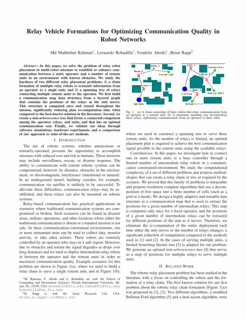
Fig. 1. (a) A chain consisting of three robots that relay communication froman operator to a remote unit; (b) A minimum spanning tree incorporatingthree relays, optimizing communication from an operator to three units.

where we need to construct a spanning tree to serve three

remote units. As the number of relays is limited, an optimal

placement plan is required to achieve the best communication

signal possible to the remote units using the available relays.

Contributions: In this paper, we investigate how to connect

one or more remote units to a base controller through a

limited number of intermediate relay robots in a communi-

cation constrained-environment. We study the computational

complexity of a set of different problems and propose method-

ologies that can create a relay chain or tree as required by the

scenario. We proved that this family of problems is intractable

and propose resolution complete algorithms that use a decom-

position of free space into a finite number of cells (such as a

grid or a mesh). We design a highly adaptive and reusable data

structure as a communication map that is used to extract the

positions for a given number of intermediate relays. This map

is computed only once for a fixed operator, and the positions

of a given number of intermediate relays can be extracted

for different positions of the unit as it moves. Therefore, we

eliminate the re-computation of the entire deployment each

time either the unit moves or the number of relays changes; a

significant reduction of computation compared to the methods

used in [1] and [2]. In the cases of serving multiple units, a

limited branching Steiner tree [3] is adapted for our problem.

We generate an optimal min-arborescence tree [4] that serves

as a map of positions for multiple relays to serve multiple

units.

II. RELATED WORK

The robotic relay placement problem has been studied in the

literature with a focus on controlling the robots and the for-

mation of a relay chain. The best known solution for our first

problem about the robotic relay chain formation (Figure 1(a))

was proposed in [1], [2]. Two different algorithms, a modified

Bellman-Ford algorithm [5] and a dual ascent algorithm, were

used on a grid to find the shortest sequence of grid points

for placing the given number of robot relays. Although their

solution is able to form a relay chain, frequent re-computation

of the chain is required each time either the unit moves to a

new location or the number of relays changes. In contrast, we

develop a reusable data structure as a static placement map that

is computed once and used to extract the new locations of the

available relays when the unit moves throughout the mission.

Thus, our solution eliminates significant re-computation and

re-planning time in a mobile robotic system.

Our second problem, multi-unit multi-relay tree formation,

is connected to the limited branching Steiner tree discussed

in [3]. Although the general problem is known to be NP-

Hard, the authors proved that a polynomial time algorithm can

compute a tree for a fixed number of branching and terminal

nodes. We have adapted the ideas in [3] for our problem

and expanded them for implementation purposes. Another

relay formation solution using Markov chains is proposed

in [6] where the relays move based on the inputs from their

neighbors. However, obstacles were not considered, and the

robots did not form other topologies besides a chain.

This research is closely related to wireless sensor networks,

mesh networks, and multi-hop dynamic wireless networks [7].

However, most of the solutions are related to area coverages

for which static relay nodes are used that are not capable

of adjusting their locations through movement. Our ideas are

naturally connected to visibility graph-based [8] planning and

art gallery problems [9], [10] that guard polygons through

visibility. However, the solution is a minimum number of

nodes required to observe the whole galley, which is not

applicable in our problem where we need to achieve the best

communication using the given number of nodes.

Our work also has similarities to leader-follower robot

formation [11], [12], [13] where a number of robots position

themselves according to the policy distributed by their leader.

Although a consensus-based control algorithm is provided

in [11] and a dynamic controller was designed in [13], no

obstacles are considered in either work. A visual odometry

is used in [12] to keep the leader in sight, but the calculated

trajectories and positions do not guarantee any optimality.

III. PRELIMINARIES

We will consider a two-dimensional environment W = R2

that is filled with polygonal obstacles O as illustrated in

Figure 1. In this environment, there is a set of m relay

vehicles A1, A2, . . . , Am and p remote units B1, B2, . . . , Bp

that need to be connected to a static operator S. We define

the collision-free space as W ′ = W \ O where the units and

relays present in the world can move freely. The remote units

are modeled as point robots and a unit Bj has configuration

space Bj , where a particular configuration rj ∈ Bj is defined

as rj = (x, y) ∈ W ′. Similarly, the configuration space for

the operator S is defined as S, where an operator’s position

s ∈ S is denoted by s = (x, y). The relay vehicles are

modeled as car-like robots and a particular vehicle Ai has

a configuration space Ci and the positions qi ∈ Ci are defined

as qi = (x, y, θ) ∈ W ′ × [0, 2π) [14].

A. Communication Quality

For any two points on the plane ρ1, ρ2 ∈ W ′, the received

power is inversely proportional to, dδ(ρ1, ρ2) [15], [16], where

d(ρ1, ρ2) is the distance between ρ1 and ρ2 and δ is the loss

coefficient. δ depends on the nature of the workspace and is

generally set to 2 when the sender (placed at ρ1) and receiver

(placed at ρ2) have free Line of Sight (LoS) (see Table 4.1

in [16]). Therefore, the free space communication cost, fFincreases with the increase of distance i.e, proportional to the

quadratic distance, d2, and is defined as,

fF (ρ1, ρ2) =

γd2(ρ1, ρ2) if d(ρ1, ρ2) < dth

∞ otherwise(1)

Here γ is a constant that depends on the transmitter [15] and

dth is the distance threshold beyond which no communication

can be established. Communication signal is further attenuated

by diffraction, fading and and/or multipath propagation effects

due to the presence of obstacles between the sender and

receiver [16].

Let the path loss in the presence of obstacles and terrain

be fO(ρ1, ρ2,O), which includes the costs resulting from

diffraction (fDF ), fading (fFA), and/or multipath propagation.

fO(ρ1, ρ2,O) =

0 if ρ1ρ2 has LoS

fDF (O) + fFA(O) otherwise

(2)

Finally, the total communication cost fC between ρ1 and

ρ2 is defined as:

fC(ρ1, ρ2) = fF (ρ1, ρ2) + fO(ρ1, ρ2,O) (3)

B. Relay Placement Problems

Our first problem of interest is to develop a solution for the

relay placement problem involving an operator, a number of

relay robots, and a remote unit. Given the operator’s position

s and a remote unit’s position r, we need to calculate a set

of relay robots’ positions q1, q2, . . . , qm such that they form a

communication chain. The communication cost is defined as,

fLC = fC(s, q1) +

∑

1≤i<m

fC(qi, qi+1) + fC(qm, r) (4)

We are required to solve the problem of creating a reusable

placement map that gives the best placements for a given num-

ber of relay vehicles. Therefore, we define a communication

map corresponding to the static operator s as M sc : B → Cn.

Accordingly, our first problem is:

Problem 1: MULTI-RELAY CHAIN - Finding Optimal

Positioning of a Set of Relay Robots on a Chain.

Given the fixed positions r and s corresponding to a unit Band an operator S, find m points q1, . . . , qm corresponding

to the m relay vehicles A1, A2, . . . , Am in the free space that

form an m+1-link m hop path to connect s to r and minimize

fLC .

We extend the multiple-relay single-unit problem to a

multiple-relay multiple-unit problem. Consequently, we have punit positions r1, . . . , rp that must be connected to s through mrelays. Therefore we define our second problem as a MULTI-

RELAY MULTI-UNIT problem:

Problem 2: MULTI-RELAY MULTI-UNIT - Finding

Optimal Positioning of a Set of Relay Robots That Serve

a Number of Remote Units.

Given a set of fixed positions r1, . . . , rp of p units and the

position s of one operator, compute the optimal positions

q1, q2, . . . , qm of m relay robots on the plane that form a

connected component among the operator, relays and units

while the term∑

1≤i≤p

min1≤j≤m

fC(ri, qj) + min1≤j≤m

fC(s, qj) is

minimized.

In this case, the optimal solution is a tree T = (V,E)that spans over the operator, p remote unit positions, and mavailable relay positions. Accordingly, the communication cost

to be minimized of this multi-unit system is defined as:

fTC (T ) =

∑

(u,v)∈E

[α1fC(u, v) + α2(deg(u) + deg(v))] (5)

where, α1 α2 ∈ [0, 1] are weighting factors such that α1 +α2 = 1. The terms deg(.) denotes the degree of a node and it

is used to constrain the number of flows/connections per node.

IV. METHODS

A. Single Unit Multiple Relay Placement

A MULTI-RELAY CHAIN problem is shown in Figure 1(a)

where we want to form a relay chain between the operator and

the remote unit. However, the problem becomes NP-Hard on

a plane filled with obstacles as stated below.Proposition 4.1: The MULTI-RELAY CHAIN problem in

a polygon with holes is NP-Hard.

Proof: (Sketch) Our problem is similar to the shortest

m+1-link paths in polygons with holes as discussed in [17],

[18]. The bi-criteria shortest path decision problem was proven

to be NP-Complete [17] when we need to decide if a path

with m + 1 links is the shortest. Therefore, the optimization

version of calculating the shortest m+1 link path (our MULTI-

RELAY CHAIN problem) is NP-Hard. Although we use a

communication cost metric fC , it is a function of the distance

metric d and does not reduce the hardness of the problem.

Therefore, we employ discretization as shown in Figure

2(a)-(b) instead of solving the problem in the continuous plane.

We convert the world W ′ = W \ O into a grid (such as a

Sukharev grid [19]) with n grid points Ω = g1, g2, . . . , gn.

An example environment grid Ω is shown in Figure 2(a)

where the operator S stays in cell 0. A graph representation

G(V,E) of Ω, based on communication cost fC , is drawn in

Figure 2(b) where the node set V is composed of all the grid

points that are not inside the obstacles O, and is defined as

V = vi|vi ≡ gi ∈ Ω and gi /∈ O. Here, a node vi ∈ Vis equivalent to a grid point gi ∈ Ω, but contains additional

attributes such as identifier, cost, neighbors, and parent. Each

node v ∈ V has a unique identifier v.id that is used to

identify the node. The set of undirected edges E is defined

as E = (u, v) : fC(u, v) < ∞ where the weight of an

edge is computed by (3). For illustration purposes, initially

the communication between two grid points is blocked by the

obstacles. However, we will show other general cases in the

experimental section where the signal is allowed to penetrate

the obstacles.

Next, we compute the communication map M sc using Algo-

rithm 1. A layered directed graph G = (V , E) with m+2 levels

l0, l1, . . . , lm+1 for m available relay robots is computed (see

Figure 2(c)) based on the original graph G. Level l0 contains

only one node v0s ≡ vs ∈ V corresponding to the static

operator’s position s which also represents the root of the tree.

Each of the subsequent layers li, where 1 ≤ i ≤ m + 1, will

copy all the nodes V \ vs of the original graph G. This means

a particular layer li contains the nodes Vi = vi1, vi2, . . . , v

i|V |

and, for a node vik ∈ Vi, the identifier vik.id = vk.id, where

vk ∈ V is the corresponding original node in G. Additionally,

the nodes at different layers with the same index have the

same identifier, which means v1k.id = v2k.id = · · · = vm+1k .id

(see Figure 2(c)). Finally, the node set V for the graph G is

defined as,

V = V0 ∪ V1 ∪ · · · ∪ Vm+1 (6)

which contains O((m + 1) · |V |) nodes. A directed edge

(u, v) ∈ E is allowed only between the nodes of any two

consecutive layers li and li+1 (lexicographic order) if and

only if (u′, v′) ∈ E (which means fC(u, v) < ∞) where

u.id = u′.id and v.id = v′.id for u′, v′ ∈ G.V :

E = (u, v) : u ∈ li, v ∈ li+1 and fC(u, v) < ∞ ; i ≤ m(7)

Once the layered graph G is constructed, we compute a

modified shortest path tree that results in our communication

map M sc . The resulting tree is constructed by exploring G

layer-wise in a lexicographic order while removing the unnec-

essary nodes that have already attained optimality. Therefore,

we modify the breadth first graph search (BFS) [5] algorithm

to explore layer by layer and compute the shortest chain from

the root vs to each of the nodes. Line 3 of Algorithm 1

initializes the exploration by enqueuing vs into a queue Q.

In order to compute the shortest path tree, we introduce a

hash table h of length |V | that uses v.id as the keys and is

initialized to ∞ (line 4). We defined earlier that a particular

node v ∈ V has the same key v.id in all the layers of Gwhere its instances appear (see the numbering in Figure 2(c)).

Therefore, h is used to keep track of the lowest cost of each

node v ∈ V of the original graph G as we explore throughout

the levels of G.

Algorithm 1 multiRelaySingleUnit(G(V,E))

1: G(V , E) = calculateGraph(G)2: vs.cost = 0, and v.parent = NULL; ∀v ∈ V3: Enqueue(Q, vs)4: h[v.id] = ∞; ∀v ∈ G.V5: while Q 6= ∅ do6: u = Dequeue(Q)7: for v ∈ u.Neighbors do8: if u.cost+ fC(u, v) < h[v.id] then9: v.parent = u

10: v.cost = u.cost+ fC(u, v)11: h[v.id] = v.cost12: Enqueue(Q, v)13: end if14: end for15: end while

Although the identifiers (v.id) of a node’s replicas across

0

2

61

3

4

9

7

5

8

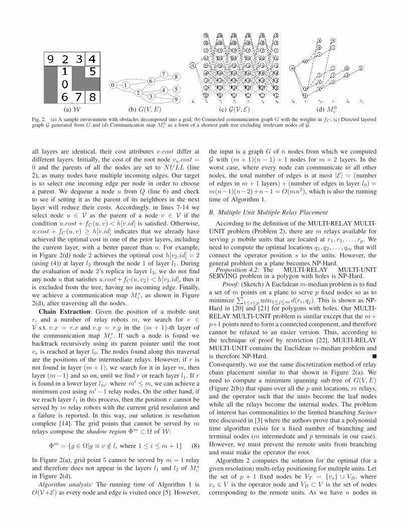
(a) W (b) G(V,E) (c) G(V , E) (d) M0c

Fig. 2. (a) A sample environment with obstacles decomposed into a grid; (b) Connected communication graph G with the weights in fC ; (c) Directed layeredgraph G generated from G and (d) Communication map M0

c as a form of a shortest path tree excluding irrelevant nodes of G.

all layers are identical, their cost attributes v.cost differ at

different layers. Initially, the cost of the root node vs.cost =0 and the parents of all the nodes are set to NULL (line

2), as many nodes have multiple incoming edges. Our target

is to select one incoming edge per node in order to choose

a parent. We dequeue a node u from Q (line 6) and check

to see if setting it as the parent of its neighbors in the next

layer will reduce their costs. Accordingly, in lines 7-14 we

select node u ∈ V as the parent of a node v ∈ V if the

condition u.cost+ fC(u, v) < h[v.id] is satisfied. Otherwise,

u.cost + fC(u, v) ≥ h[v.id] indicates that we already have

achieved the optimal cost in one of the prior layers, including

the current layer, with a better parent than u. For example,

in Figure 2(d) node 2 achieves the optimal cost h[v2.id] = 2(using (4)) at layer l2 through the node 1 of layer l1. During

the evaluation of node 2’s replica in layer l3, we do not find

any node u that satisfies u.cost+fC(u, v2) < h[v2.id], thus it

is excluded from the tree, having no incoming edge. Finally,

we achieve a communication map M sc , as shown in Figure

2(d), after traversing all the nodes.

Chain Extraction: Given the position of a mobile unit

r, and a number of relay robots m, we search for v ∈V s.t. v.x = r.x and v.y = r.y in the (m + 1)-th layer of

the communication map M sc . If such a node is found we

backtrack recursively using its parent pointer until the root

vs is reached at layer l0. The nodes found along this traversal

are the positions of the intermediate relays. However, if r is

not found in layer (m+ 1), we search for it in layer m, then

layer (m−1) and so on, until we find r or reach layer l1. If ris found in a lower layer lm′ where m′ ≤ m, we can achieve a

minimum cost using m′−1 relay nodes. On the other hand, if

we reach layer l1 in this process, then the position r cannot be

served by m relay robots with the current grid resolution and

a failure is reported. In this way, our solution is resolution

complete [14]. The grid points that cannot be served by mrelays compose the shadow region Φm ⊂ Ω of W :

Φm = g ∈ Ω|g ≡ v /∈ li where 1 ≤ i ≤ m+ 1 (8)

In Figure 2(a), grid point 5 cannot be served by m = 1 relay

and therefore does not appear in the layers l1 and l2 of M sc

in Figure 2(d).

Algorithm analysis: The running time of Algorithm 1 is

O(V+E) as every node and edge is visited once [5]. However,

the input is a graph G of n nodes from which we computed

G with (m + 1)(n − 1) + 1 nodes for m + 2 layers. In the

worst case, where every node can communicate to all other

nodes, the total number of edges is at most |E| = (number

of edges in m+ 1 layers) + (number of edges in layer l0) =m(n−1)(n−2)+n−1 = O(mn2), which is also the running

time of Algorithm 1.

B. Multiple Unit Multiple Relay Placement

According to the definition of the MULTI-RELAY MULTI-

UNIT problem (Problem 2), there are m relays available for

serving p mobile units that are located at r1, r2, . . . , rp. We

need to compute the optimal locations q1, q2, . . . , qm that will

connect the operator position s to the units. However, the

general problem on a plane becomes NP-Hard.Proposition 4.2: The MULTI-RELAY MULTI-UNIT

SERVING problem in a polygon with holes is NP-Hard.

Proof: (Sketch) A Euclidean m-median problem is to find

a set of m points on a plane to serve p fixed nodes so as to

minimize∑

1≤i≤p min1≤j≤m d(ri, qj). This is shown as NP-

Hard in [20] and [21] for polygons with holes. Our MULTI-

RELAY MULTI-UNIT problem is similar except that the m+p+1 points need to form a connected component, and therefore

cannot be relaxed to an easier version. Thus, according to

the technique of proof by restriction [22], MULTI-RELAY

MULTI-UNIT contains the Euclidean m-median problem and

is therefore NP-Hard.

Consequently, we use the same discretization method of relay

chain placement similar to that shown in Figure 2(a). We

need to compute a minimum spanning sub-tree of G(V,E)(Figure 2(b)) that spans over all the p unit locations, m relays,

and the operator such that the units become the leaf nodes

while all the relays become the internal nodes. The problem

of interest has commonalities to the limited branching Steiner

tree discussed in [3] where the authors prove that a polynomial

time algorithm exists for a fixed number of branching and

terminal nodes (m intermediate and p terminals in our case).

However, we must prevent the remote units from branching

and must make the operator the root.

Algorithm 2 computes the solution for the optimal (for a

given resolution) multi-relay positioning for multiple units. Let

the set of p + 1 fixed nodes be VT = vs ∪ VB , where

vs ∈ V is the operator node and VB ⊂ V is the set of nodes

corresponding to the remote units. As we have n nodes in

02

1

4

9

0 1 24

90 2 3

9

4

0 23

9

4

(a) (b) (c) (d)

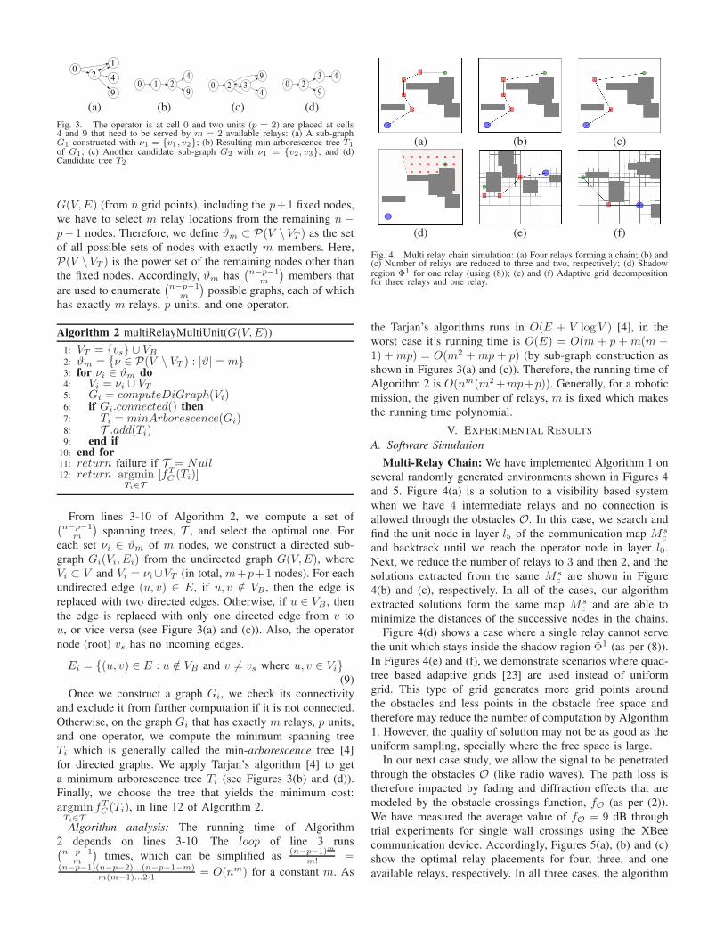
Fig. 3. The operator is at cell 0 and two units (p = 2) are placed at cells4 and 9 that need to be served by m = 2 available relays: (a) A sub-graphG1 constructed with ν1 = v1, v2; (b) Resulting min-arborescence tree T1

of G1; (c) Another candidate sub-graph G2 with ν1 = v2, v3; and (d)Candidate tree T2

G(V,E) (from n grid points), including the p+1 fixed nodes,

we have to select m relay locations from the remaining n −p− 1 nodes. Therefore, we define ϑm ⊂ P(V \VT ) as the set

of all possible sets of nodes with exactly m members. Here,

P(V \VT ) is the power set of the remaining nodes other than

the fixed nodes. Accordingly, ϑm has(

n−p−1m

)

members that

are used to enumerate(

n−p−1m

)

possible graphs, each of which

has exactly m relays, p units, and one operator.

Algorithm 2 multiRelayMultiUnit(G(V,E))

1: VT = vs ∪ VB

2: ϑm = ν ∈ P(V \ VT ) : |ϑ| = m3: for νi ∈ ϑm do4: Vi = νi ∪ VT5: Gi = computeDiGraph(Vi)6: if Gi.connected() then7: Ti = minArborescence(Gi)8: T .add(Ti)9: end if

10: end for11: return failure if T = Null12: return argmin

Ti∈T[fT

C (Ti)]

From lines 3-10 of Algorithm 2, we compute a set of(

n−p−1m

)

spanning trees, T , and select the optimal one. For

each set νi ∈ ϑm of m nodes, we construct a directed sub-

graph Gi(Vi, Ei) from the undirected graph G(V,E), where

Vi ⊂ V and Vi = νi∪VT (in total, m+p+1 nodes). For each

undirected edge (u, v) ∈ E, if u, v /∈ VB , then the edge is

replaced with two directed edges. Otherwise, if u ∈ VB , then

the edge is replaced with only one directed edge from v to

u, or vice versa (see Figure 3(a) and (c)). Also, the operator

node (root) vs has no incoming edges.

Ei = (u, v) ∈ E : u /∈ VB and v 6= vs where u, v ∈ Vi(9)

Once we construct a graph Gi, we check its connectivity

and exclude it from further computation if it is not connected.

Otherwise, on the graph Gi that has exactly m relays, p units,

and one operator, we compute the minimum spanning tree

Ti which is generally called the min-arborescence tree [4]

for directed graphs. We apply Tarjan’s algorithm [4] to get

a minimum arborescence tree Ti (see Figures 3(b) and (d)).

Finally, we choose the tree that yields the minimum cost:

argminTi∈T

fTC (Ti), in line 12 of Algorithm 2.

Algorithm analysis: The running time of Algorithm

2 depends on lines 3-10. The loop of line 3 runs(

n−p−1m

)

times, which can be simplified as(n−p−1)m

m! =(n−p−1)(n−p−2)...(n−p−1−m)

m(m−1)...2·1 = O(nm) for a constant m. As

(a) (b) (c)

(d) (e) (f)

Fig. 4. Multi relay chain simulation: (a) Four relays forming a chain; (b) and(c) Number of relays are reduced to three and two, respectively; (d) Shadowregion Φ1 for one relay (using (8)); (e) and (f) Adaptive grid decompositionfor three relays and one relay.

the Tarjan’s algorithms runs in O(E + V logV ) [4], in the

worst case it’s running time is O(E) = O(m + p +m(m −1) +mp) = O(m2 +mp + p) (by sub-graph construction as

shown in Figures 3(a) and (c)). Therefore, the running time of

Algorithm 2 is O(nm(m2+mp+p)). Generally, for a robotic

mission, the given number of relays, m is fixed which makes

the running time polynomial.

V. EXPERIMENTAL RESULTS

A. Software Simulation

Multi-Relay Chain: We have implemented Algorithm 1 on

several randomly generated environments shown in Figures 4

and 5. Figure 4(a) is a solution to a visibility based system

when we have 4 intermediate relays and no connection is

allowed through the obstacles O. In this case, we search and

find the unit node in layer l5 of the communication map M sc

and backtrack until we reach the operator node in layer l0.

Next, we reduce the number of relays to 3 and then 2, and the

solutions extracted from the same M sc are shown in Figure

4(b) and (c), respectively. In all of the cases, our algorithm

extracted solutions form the same map M sc and are able to

minimize the distances of the successive nodes in the chains.

Figure 4(d) shows a case where a single relay cannot serve

the unit which stays inside the shadow region Φ1 (as per (8)).

In Figures 4(e) and (f), we demonstrate scenarios where quad-

tree based adaptive grids [23] are used instead of uniform

grid. This type of grid generates more grid points around

the obstacles and less points in the obstacle free space and

therefore may reduce the number of computation by Algorithm

1. However, the quality of solution may not be as good as the

uniform sampling, specially where the free space is large.

In our next case study, we allow the signal to be penetrated

through the obstacles O (like radio waves). The path loss is

therefore impacted by fading and diffraction effects that are

modeled by the obstacle crossings function, fO (as per (2)).

We have measured the average value of fO = 9 dB through

trial experiments for single wall crossings using the XBee

communication device. Accordingly, Figures 5(a), (b) and (c)

show the optimal relay placements for four, three, and one

available relays, respectively. In all three cases, the algorithm

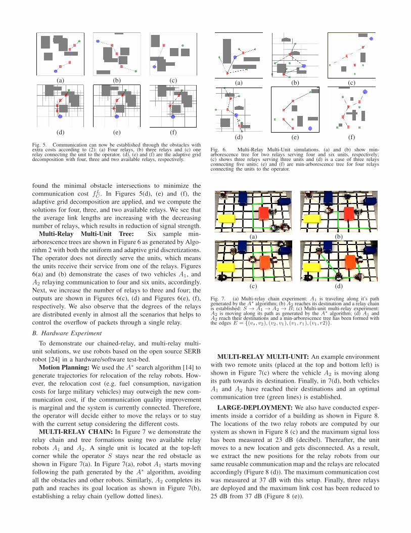
(a) (b) (c)

(d) (e) (f)

Fig. 5. Communication can now be established through the obstacles withextra costs according to (2): (a) Four relays, (b) three relays and (c) onerelay connecting the unit to the operator. (d), (e) and (f) are the adaptive griddecomposition with four, three and two available relays, respectively.

found the minimal obstacle intersections to minimize the

communication cost fLC . In Figures 5(d), (e) and (f), the

adaptive grid decomposition are applied, and we compute the

solutions for four, three, and two available relays. We see that

the average link lengths are increasing with the decreasing

number of relays, which results in reduction of signal strength.

Multi-Relay Multi-Unit Tree: Six sample min-

arborescence trees are shown in Figure 6 as generated by Algo-

rithm 2 with both the uniform and adaptive grid discretizations.

The operator does not directly serve the units, which means

the units receive their service from one of the relays. Figures

6(a) and (b) demonstrate the cases of two vehicles A1, and

A2 relaying communication to four and six units, accordingly.

Next, we increase the number of relays to three and four; the

outputs are shown in Figures 6(c), (d) and Figures 6(e), (f),

respectively. We also observe that the degrees of the relays

are distributed evenly in almost all the scenarios that helps to

control the overflow of packets through a single relay.

B. Hardware Experiment

To demonstrate our chained-relay, and multi-relay multi-

unit solutions, we use robots based on the open source SERB

robot [24] in a hardware/software test-bed.

Motion Planning: We used the A∗ search algorithm [14] to

generate trajectories for relocation of the relay robots. How-

ever, the relocation cost (e.g. fuel consumption, navigation

costs for large military vehicles) may outweigh the new com-

munication cost, if the communication quality improvement

is marginal and the system is currently connected. Therefore,

the operator will decide either to move the relays or to stay

with the current setup considering the different costs.

MULTI-RELAY CHAIN: In Figure 7 we demonstrate the

relay chain and tree formations using two available relay

robots A1 and A2. A single unit is located at the top-left

corner while the operator S stays near the red obstacle as

shown in Figure 7(a). In Figure 7(a), robot A1 starts moving

following the path generated by the A∗ algorithm, avoiding

all the obstacles and other robots. Similarly, A2 completes its

path and reaches its goal location as shown in Figure 7(b),

establishing a relay chain (yellow dotted lines).

(a) (b) (c)

(d) (e) (f)

Fig. 6. Multi-Relay Multi-Unit simulations. (a) and (b) show min-arborescence tree for two relays serving four and six units, respectively;(c) shows three relays serving three units and (d) is a case of three relaysconnecting five units; (e) and (f) are min-arborescence tree for four relaysconnecting the units to the operator.

(a) (b)

(c) (d)

Fig. 7. (a) Multi-relay chain experiment: A1 is traveling along it’s pathgenerated by the A∗ algorithm; (b) A2 reaches its destination and a relay chainis established: S → A1 → A2 → B; (c) Multi-unit multi-relay experiment:A2 is moving along its path as generated by the A∗ algorithm; (d) A1 andA2 reach their destinations and a min-arborescence tree has been formed withthe edges E = (vs , v2), (v2, v1), (v1, r1), (v1, r2).

MULTI-RELAY MULTI-UNIT: An example environment

with two remote units (placed at the top and bottom left) is

shown in Figure 7(c) where the vehicle A2 is moving along

its path towards its destination. Finally, in 7(d), both vehicles

A1 and A2 have reached their destinations and an optimal

communication tree (green lines) is established.

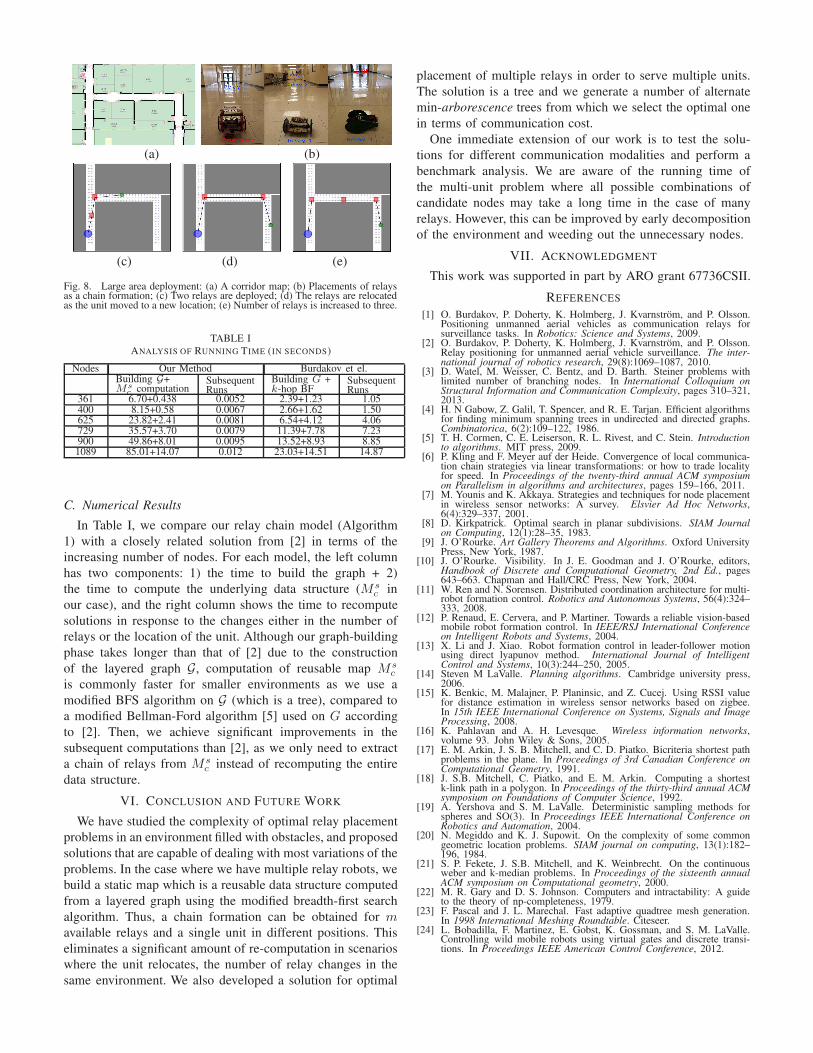
LARGE-DEPLOYMENT: We also have conducted exper-

iments inside a corridor of a building as shown in Figure 8.

The locations of the two relay robots are computed by our

system as shown in Figure 8 (c) and the maximum signal loss

has been measured at 23 dB (decibel). Thereafter, the unit

moves to a new location and gets disconnected. As a result,

we extract the new positions for the relay robots from our

same reusable communication map and the relays are relocated

accordingly (Figure 8 (d)). The maximum communication cost

was measured at 37 dB with this setup. Finally, three relays

are deployed and the maximum link cost has been reduced to

25 dB from 37 dB (Figure 8 (e)).

(a) (b)

(c) (d) (e)

Fig. 8. Large area deployment: (a) A corridor map; (b) Placements of relaysas a chain formation; (c) Two relays are deployed; (d) The relays are relocatedas the unit moved to a new location; (e) Number of relays is increased to three.

TABLE I

ANALYSIS OF RUNNING TIME (IN SECONDS)

Nodes Our Method Burdakov et el.Building G+Ms

c computationSubsequentRuns

Building G +k-hop BF

SubsequentRuns

361 6.70+0.438 0.0052 2.39+1.23 1.05400 8.15+0.58 0.0067 2.66+1.62 1.50625 23.82+2.41 0.0081 6.54+4.12 4.06729 35.57+3.70 0.0079 11.39+7.78 7.23900 49.86+8.01 0.0095 13.52+8.93 8.851089 85.01+14.07 0.012 23.03+14.51 14.87

C. Numerical Results

In Table I, we compare our relay chain model (Algorithm

1) with a closely related solution from [2] in terms of the

increasing number of nodes. For each model, the left column

has two components: 1) the time to build the graph + 2)

the time to compute the underlying data structure (M sc in

our case), and the right column shows the time to recompute

solutions in response to the changes either in the number of

relays or the location of the unit. Although our graph-building

phase takes longer than that of [2] due to the construction

of the layered graph G, computation of reusable map M sc

is commonly faster for smaller environments as we use a

modified BFS algorithm on G (which is a tree), compared to

a modified Bellman-Ford algorithm [5] used on G according

to [2]. Then, we achieve significant improvements in the

subsequent computations than [2], as we only need to extract

a chain of relays from M sc instead of recomputing the entire

data structure.

VI. CONCLUSION AND FUTURE WORK

We have studied the complexity of optimal relay placement

problems in an environment filled with obstacles, and proposed

solutions that are capable of dealing with most variations of the

problems. In the case where we have multiple relay robots, we

build a static map which is a reusable data structure computed

from a layered graph using the modified breadth-first search

algorithm. Thus, a chain formation can be obtained for mavailable relays and a single unit in different positions. This

eliminates a significant amount of re-computation in scenarios

where the unit relocates, the number of relay changes in the

same environment. We also developed a solution for optimal

placement of multiple relays in order to serve multiple units.

The solution is a tree and we generate a number of alternate

min-arborescence trees from which we select the optimal one

in terms of communication cost.

One immediate extension of our work is to test the solu-

tions for different communication modalities and perform a

benchmark analysis. We are aware of the running time of

the multi-unit problem where all possible combinations of

candidate nodes may take a long time in the case of many

relays. However, this can be improved by early decomposition

of the environment and weeding out the unnecessary nodes.

VII. ACKNOWLEDGMENT

This work was supported in part by ARO grant 67736CSII.

REFERENCES

[1] O. Burdakov, P. Doherty, K. Holmberg, J. Kvarnstrom, and P. Olsson.Positioning unmanned aerial vehicles as communication relays forsurveillance tasks. In Robotics: Science and Systems, 2009.

[2] O. Burdakov, P. Doherty, K. Holmberg, J. Kvarnstrom, and P. Olsson.Relay positioning for unmanned aerial vehicle surveillance. The inter-national journal of robotics research, 29(8):1069–1087, 2010.

[3] D. Watel, M. Weisser, C. Bentz, and D. Barth. Steiner problems withlimited number of branching nodes. In International Colloquium onStructural Information and Communication Complexity, pages 310–321,2013.

[4] H. N Gabow, Z. Galil, T. Spencer, and R. E. Tarjan. Efficient algorithmsfor finding minimum spanning trees in undirected and directed graphs.Combinatorica, 6(2):109–122, 1986.

[5] T. H. Cormen, C. E. Leiserson, R. L. Rivest, and C. Stein. Introductionto algorithms. MIT press, 2009.

[6] P. Kling and F. Meyer auf der Heide. Convergence of local communica-tion chain strategies via linear transformations: or how to trade localityfor speed. In Proceedings of the twenty-third annual ACM symposiumon Parallelism in algorithms and architectures, pages 159–166, 2011.

[7] M. Younis and K. Akkaya. Strategies and techniques for node placementin wireless sensor networks: A survey. Elsvier Ad Hoc Networks,6(4):329–337, 2001.

[8] D. Kirkpatrick. Optimal search in planar subdivisions. SIAM Journalon Computing, 12(1):28–35, 1983.

[9] J. O’Rourke. Art Gallery Theorems and Algorithms. Oxford UniversityPress, New York, 1987.

[10] J. O’Rourke. Visibility. In J. E. Goodman and J. O’Rourke, editors,Handbook of Discrete and Computational Geometry, 2nd Ed., pages643–663. Chapman and Hall/CRC Press, New York, 2004.

[11] W. Ren and N. Sorensen. Distributed coordination architecture for multi-robot formation control. Robotics and Autonomous Systems, 56(4):324–333, 2008.

[12] P. Renaud, E. Cervera, and P. Martiner. Towards a reliable vision-basedmobile robot formation control. In IEEE/RSJ International Conferenceon Intelligent Robots and Systems, 2004.

[13] X. Li and J. Xiao. Robot formation control in leader-follower motionusing direct lyapunov method. International Journal of IntelligentControl and Systems, 10(3):244–250, 2005.

[14] Steven M LaValle. Planning algorithms. Cambridge university press,2006.

[15] K. Benkic, M. Malajner, P. Planinsic, and Z. Cucej. Using RSSI valuefor distance estimation in wireless sensor networks based on zigbee.In 15th IEEE International Conference on Systems, Signals and ImageProcessing, 2008.

[16] K. Pahlavan and A. H. Levesque. Wireless information networks,volume 93. John Wiley & Sons, 2005.

[17] E. M. Arkin, J. S. B. Mitchell, and C. D. Piatko. Bicriteria shortest pathproblems in the plane. In Proceedings of 3rd Canadian Conference onComputational Geometry, 1991.

[18] J. S.B. Mitchell, C. Piatko, and E. M. Arkin. Computing a shortestk-link path in a polygon. In Proceedings of the thirty-third annual ACMsymposium on Foundations of Computer Science, 1992.

[19] A. Yershova and S. M. LaValle. Deterministic sampling methods forspheres and SO(3). In Proceedings IEEE International Conference onRobotics and Automation, 2004.

[20] N. Megiddo and K. J. Supowit. On the complexity of some commongeometric location problems. SIAM journal on computing, 13(1):182–196, 1984.

[21] S. P. Fekete, J. S.B. Mitchell, and K. Weinbrecht. On the continuousweber and k-median problems. In Proceedings of the sixteenth annualACM symposium on Computational geometry, 2000.

[22] M. R. Gary and D. S. Johnson. Computers and intractability: A guideto the theory of np-completeness, 1979.

[23] F. Pascal and J. L. Marechal. Fast adaptive quadtree mesh generation.In 1998 International Meshing Roundtable. Citeseer.

[24] L. Bobadilla, F. Martinez, E. Gobst, K. Gossman, and S. M. LaValle.Controlling wild mobile robots using virtual gates and discrete transi-tions. In Proceedings IEEE American Control Conference, 2012.