Embed Size (px)
Citation preview
Relaxation approximation
for hyperbolic fluid systems
Nicolas Seguin
Frédéric Coquel Edwige Godlewski
Laboratoire Jacques-Louis LionsUniversité Pierre et Marie Curie – Paris 6
Multimat 07, Praha
Relaxation approximation for hyperbolic fluid systems – p. 1/32
Outline of the talk
⊲ The relaxation phenomenon⊲ Principles⊲ Bibliography
⊲ Theoretical relaxation approximation⊲ The case of the Burgers equation⊲ Gas dynamics equations⊲ Hyperbolic fluid systems
⊲ Numerical schemes using the relaxation approximation⊲ Finite volume schemes and Godunov-type schemes⊲ Numerical relaxation⊲ Properties of relaxation schemes
⊲ Conclusion
Relaxation approximation for hyperbolic fluid systems – p. 2/32
The relaxation phenomenon
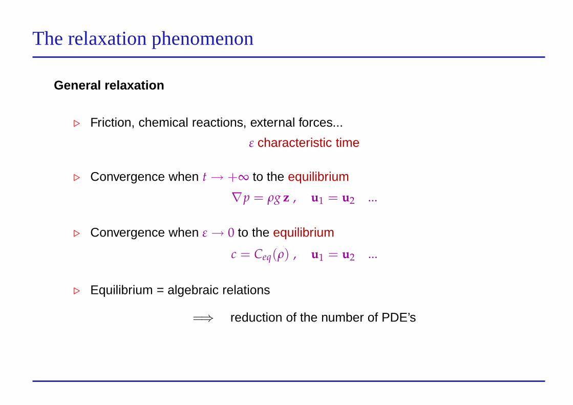
General relaxation
⊲ Friction, chemical reactions, external forces...
ε characteristic time
⊲ Convergence when t→ +∞ to the equilibrium
∇p = ρg z , u1 = u2 ...
⊲ Convergence when ε→ 0 to the equilibrium
c = Ceq(ρ) , u1 = u2 ...
⊲ Equilibrium = algebraic relations
=⇒ reduction of the number of PDE’s
Relaxation approximation for hyperbolic fluid systems – p. 3/32
The relaxation phenomenon
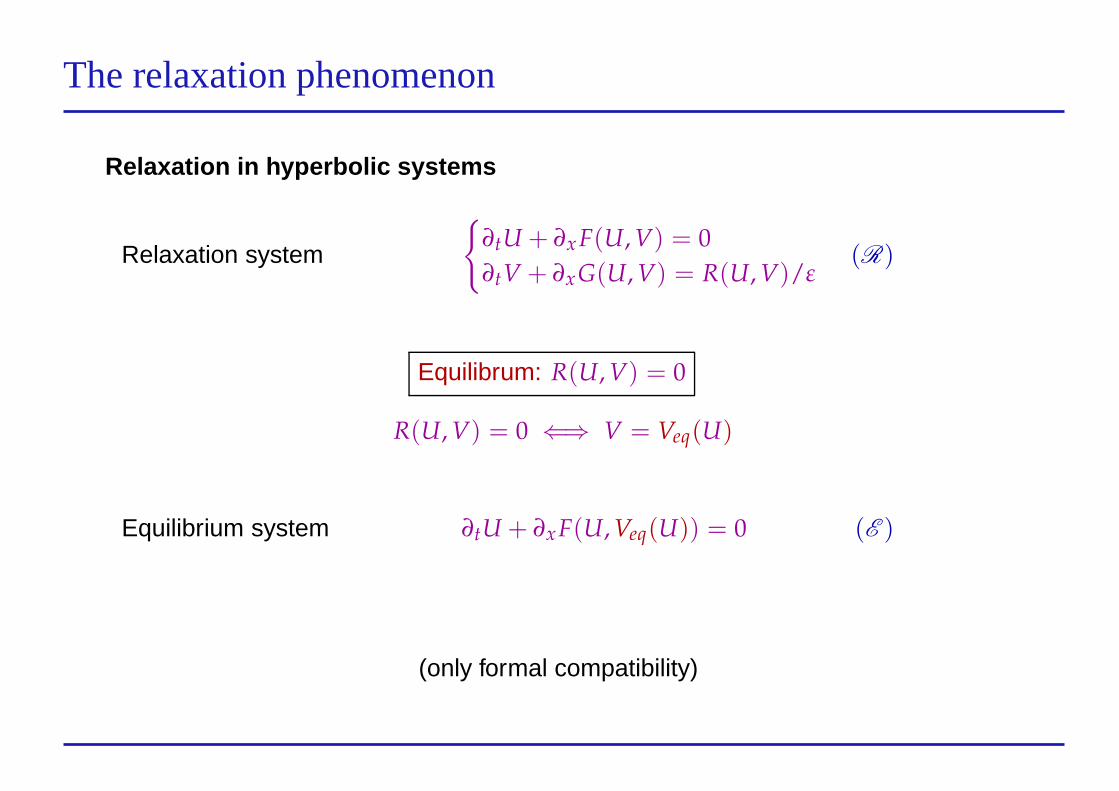
Relaxation in hyperbolic systems
Relaxation system
{
∂tU + ∂x F(U, V) = 0
∂tV + ∂xG(U, V) = R(U, V)/ε(R)
Equilibrum: R(U, V) = 0
R(U, V) = 0 ⇐⇒ V = Veq(U)
Equilibrium system ∂tU + ∂xF(U, Veq(U)) = 0 (E )
(only formal compatibility)
Relaxation approximation for hyperbolic fluid systems – p. 4/32
The relaxation approximation
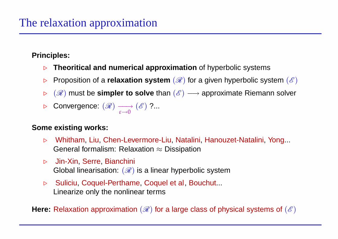
Principles:
⊲ Theoritical and numerical approximation of hyperbolic systems
⊲ Proposition of a relaxation system (R) for a given hyperbolic system (E )
⊲ (R) must be simpler to solve than (E ) −→ approximate Riemann solver
⊲ Convergence: (R) −−→ε→0
(E ) ?...
Some existing works:
⊲ Whitham, Liu, Chen-Levermore-Liu, Natalini, Hanouzet-Natalini, Yong...General formalism: Relaxation ≈ Dissipation
⊲ Jin-Xin, Serre, BianchiniGlobal linearisation: (R) is a linear hyperbolic system
⊲ Suliciu, Coquel-Perthame, Coquel et al, Bouchut...Linearize only the nonlinear terms
Here: Relaxation approximation (R) for a large class of physical systems of (E )
Relaxation approximation for hyperbolic fluid systems – p. 5/32
The Jin-Xin approximation for a conservation law
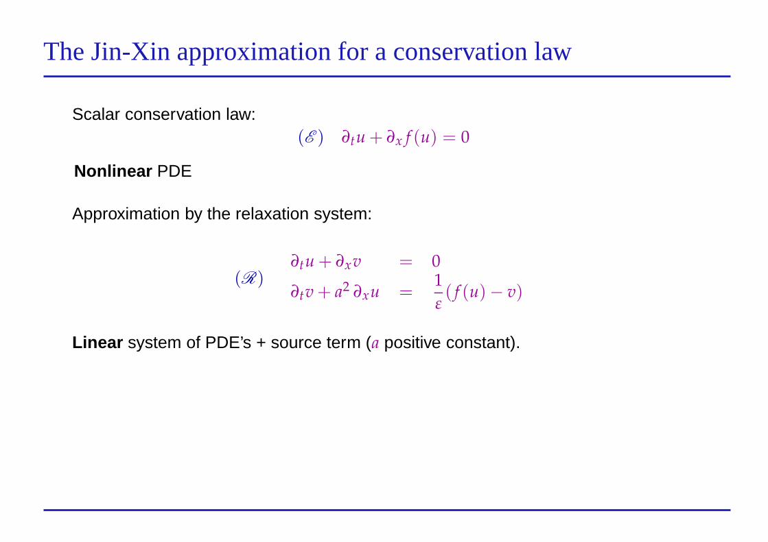
Scalar conservation law:(E ) ∂tu + ∂x f (u) = 0
Nonlinear PDE
Approximation by the relaxation system:
(R)∂tu + ∂xv = 0
∂tv + a2 ∂xu =1
ε( f (u)− v)
Linear system of PDE’s + source term (a positive constant).
Relaxation approximation for hyperbolic fluid systems – p. 6/32
The Jin-Xin approximation for a conservation law
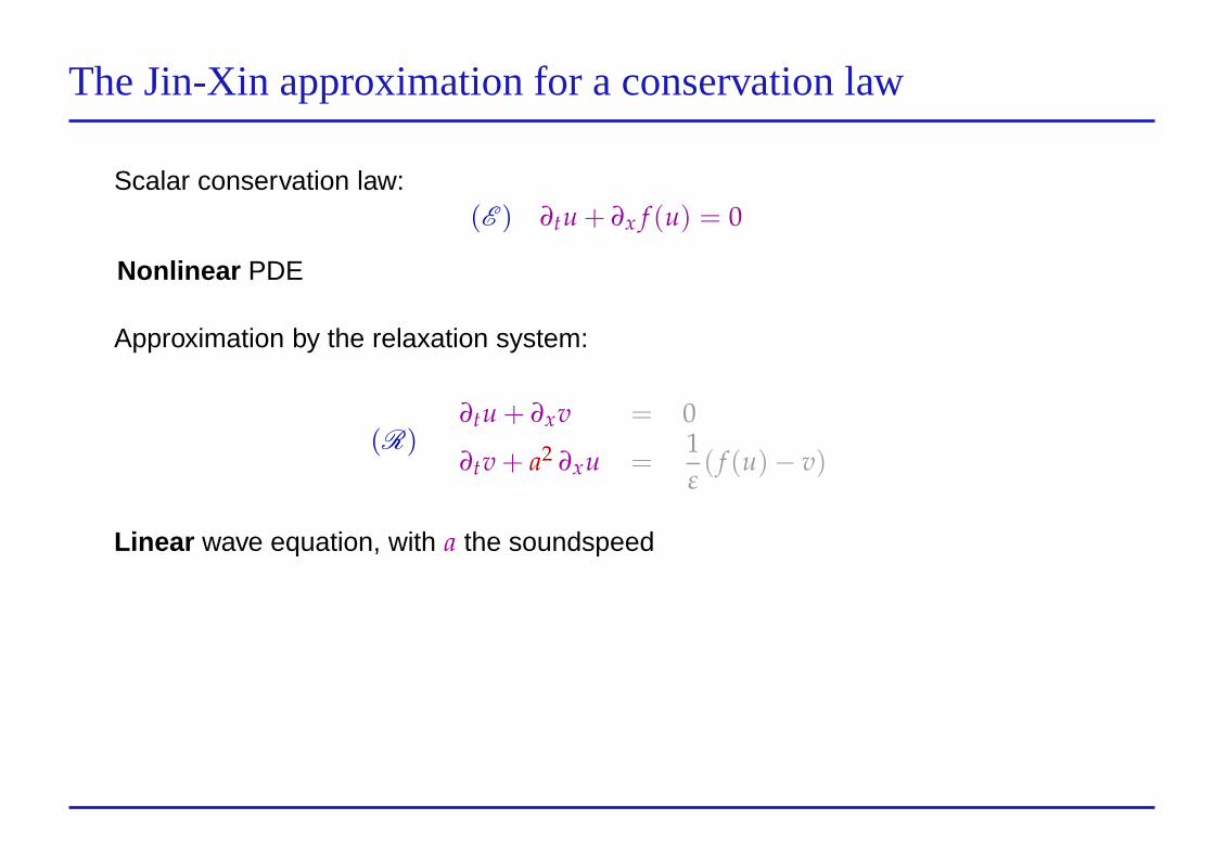
Scalar conservation law:(E ) ∂tu + ∂x f (u) = 0
Nonlinear PDE
Approximation by the relaxation system:
(R)∂tu + ∂xv = 0
∂tv + a2 ∂xu =1
ε( f (u)− v)
Linear wave equation, with a the soundspeed
Relaxation approximation for hyperbolic fluid systems – p. 7/32
The Jin-Xin approximation for a conservation law
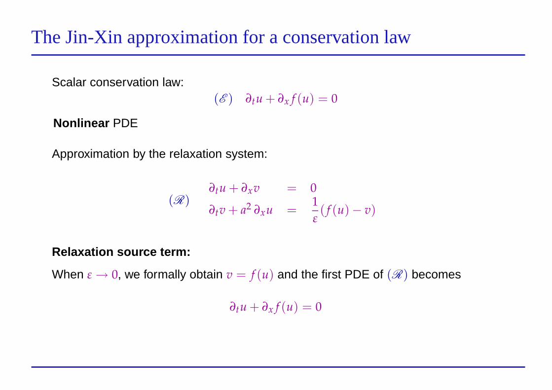
Scalar conservation law:(E ) ∂tu + ∂x f (u) = 0
Nonlinear PDE
Approximation by the relaxation system:
(R)∂tu + ∂xv = 0
∂tv + a2 ∂xu =1
ε( f (u)− v)
Relaxation source term:
When ε→ 0, we formally obtain v = f (u) and the first PDE of (R) becomes
∂tu + ∂x f (u) = 0
Relaxation approximation for hyperbolic fluid systems – p. 8/32
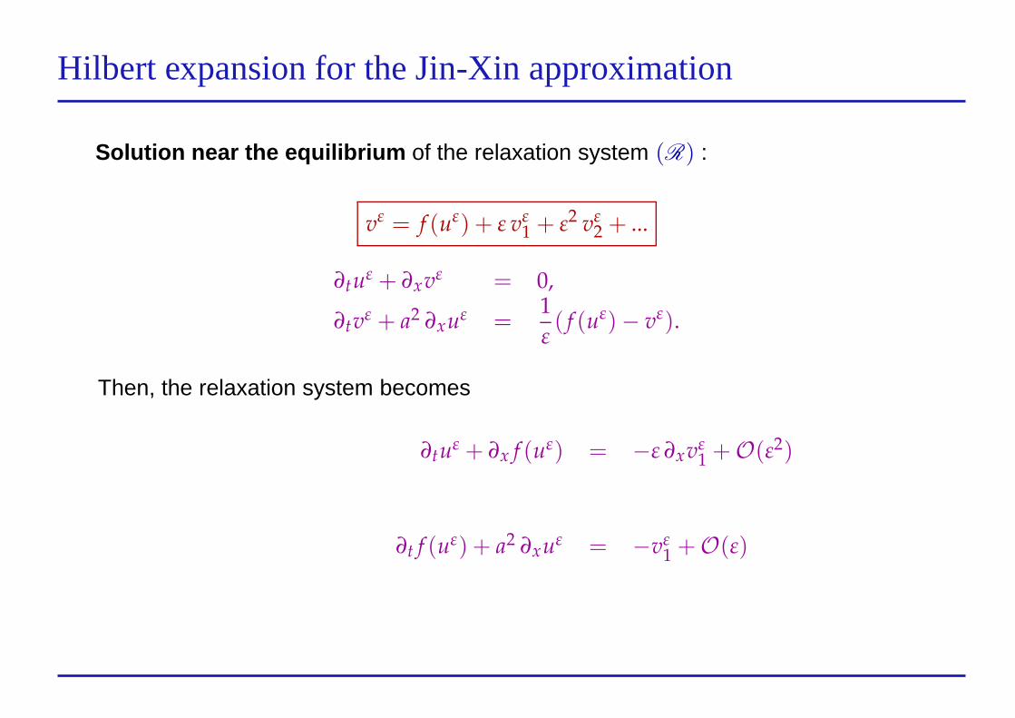
Hilbert expansion for the Jin-Xin approximation
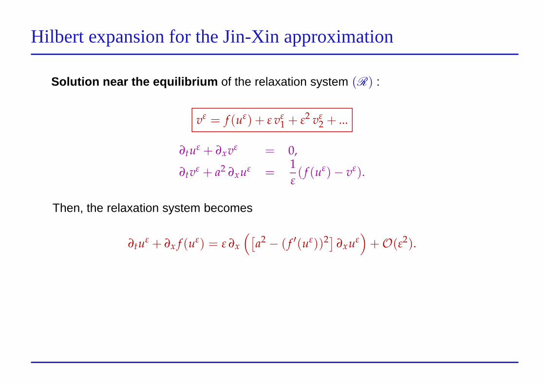
Solution near the equilibrium of the relaxation system (R) :
vε = f (uε) + ε vε1 + ε2 vε
2 + ...
∂tuε + ∂xvε = 0,
∂tvε + a2 ∂xuε =
1
ε( f (uε)− vε).
Then, the relaxation system becomes
∂tuε + ∂x f (uε) = −ε ∂xvε
1 +O(ε2)
∂t f (uε) + a2 ∂xuε = −vε1 +O(ε)
Relaxation approximation for hyperbolic fluid systems – p. 9/32
Hilbert expansion for the Jin-Xin approximation
Solution near the equilibrium of the relaxation system (R) :
vε = f (uε) + ε vε1 + ε2 vε
2 + ...
∂tuε + ∂xvε = 0,
∂tvε + a2 ∂xuε =
1
ε( f (uε)− vε).
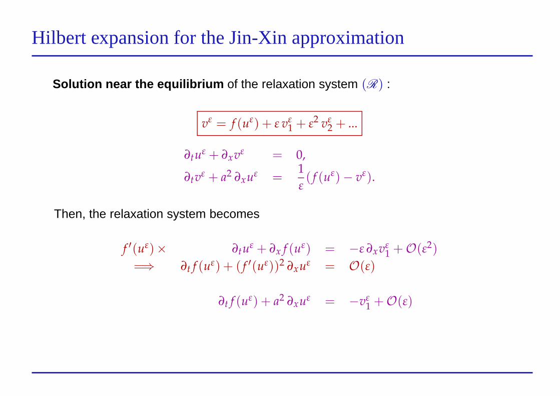
Then, the relaxation system becomes
f ′(uε)× ∂tuε + ∂x f (uε) = −ε ∂xvε
1 +O(ε2)
=⇒ ∂t f (uε) + ( f ′(uε))2 ∂xuε = O(ε)
∂t f (uε) + a2 ∂xuε = −vε1 +O(ε)
Relaxation approximation for hyperbolic fluid systems – p. 10/32
Hilbert expansion for the Jin-Xin approximation
Solution near the equilibrium of the relaxation system (R) :
vε = f (uε) + ε vε1 + ε2 vε
2 + ...
∂tuε + ∂xvε = 0,
∂tvε + a2 ∂xuε =
1
ε( f (uε)− vε).
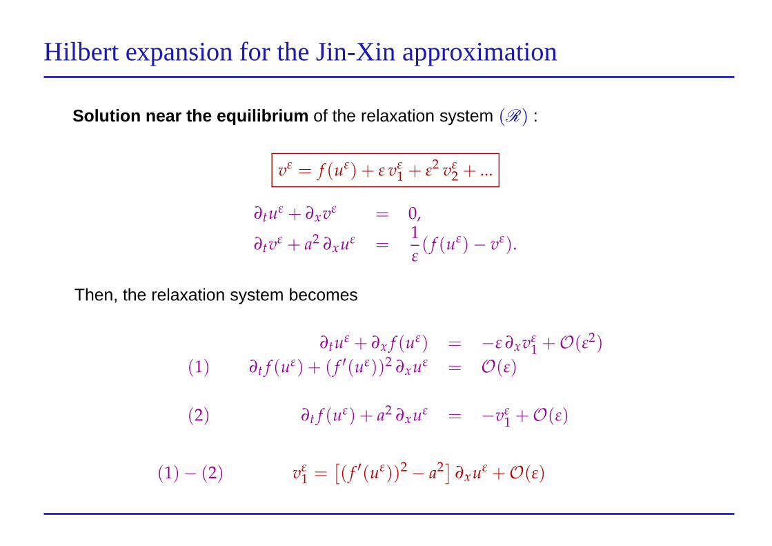
Then, the relaxation system becomes
∂tuε + ∂x f (uε) = −ε ∂xvε
1 +O(ε2)
(1) ∂t f (uε) + ( f ′(uε))2 ∂xuε = O(ε)
(2) ∂t f (uε) + a2 ∂xuε = −vε1 +O(ε)
(1)− (2) vε1 =
[
( f ′(uε))2 − a2]
∂xuε +O(ε)
Relaxation approximation for hyperbolic fluid systems – p. 11/32
Hilbert expansion for the Jin-Xin approximation
Solution near the equilibrium of the relaxation system (R) :
vε = f (uε) + ε vε1 + ε2 vε
2 + ...
∂tuε + ∂xvε = 0,
∂tvε + a2 ∂xuε =
1
ε( f (uε)− vε).
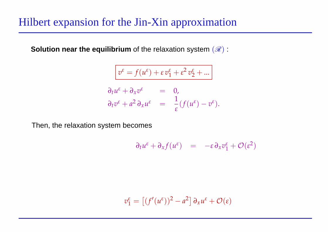
Then, the relaxation system becomes
∂tuε + ∂x f (uε) = −ε ∂xvε
1 +O(ε2)
vε1 =
[
( f ′(uε))2 − a2]
∂xuε +O(ε)
Relaxation approximation for hyperbolic fluid systems – p. 12/32
Hilbert expansion for the Jin-Xin approximation
Solution near the equilibrium of the relaxation system (R) :
vε = f (uε) + ε vε1 + ε2 vε
2 + ...
∂tuε + ∂xvε = 0,
∂tvε + a2 ∂xuε =
1
ε( f (uε)− vε).
Then, the relaxation system becomes
∂tuε + ∂x f (uε) = ε ∂x
(
[
a2 − ( f ′(uε))2]
∂xuε)
+O(ε2).
Relaxation approximation for hyperbolic fluid systems – p. 13/32
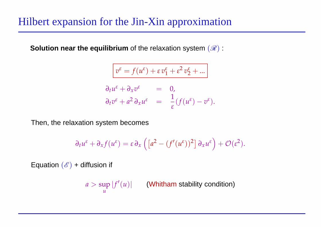
Hilbert expansion for the Jin-Xin approximation
Solution near the equilibrium of the relaxation system (R) :
vε = f (uε) + ε vε1 + ε2 vε
2 + ...
∂tuε + ∂xvε = 0,
∂tvε + a2 ∂xuε =
1
ε( f (uε)− vε).
Then, the relaxation system becomes
∂tuε + ∂x f (uε) = ε ∂x
(
[
a2 − ( f ′(uε))2]
∂xuε)
+O(ε2).
Equation (E ) + diffusion if
a > supu| f ′(u)| (Whitham stability condition)
Relaxation approximation for hyperbolic fluid systems – p. 14/32
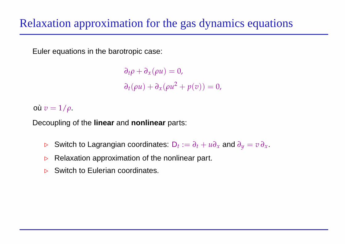
Relaxation approximation for the gas dynamics equations
Euler equations in the barotropic case:
∂tρ + ∂x(ρu) = 0,
∂t(ρu) + ∂x(ρu2 + p(v)) = 0,
où v = 1/ρ.
Decoupling of the linear and nonlinear parts:
⊲ Switch to Lagrangian coordinates: Dt := ∂t + u∂x and ∂y = v ∂x.
⊲ Relaxation approximation of the nonlinear part.
⊲ Switch to Eulerian coordinates.
Relaxation approximation for hyperbolic fluid systems – p. 15/32
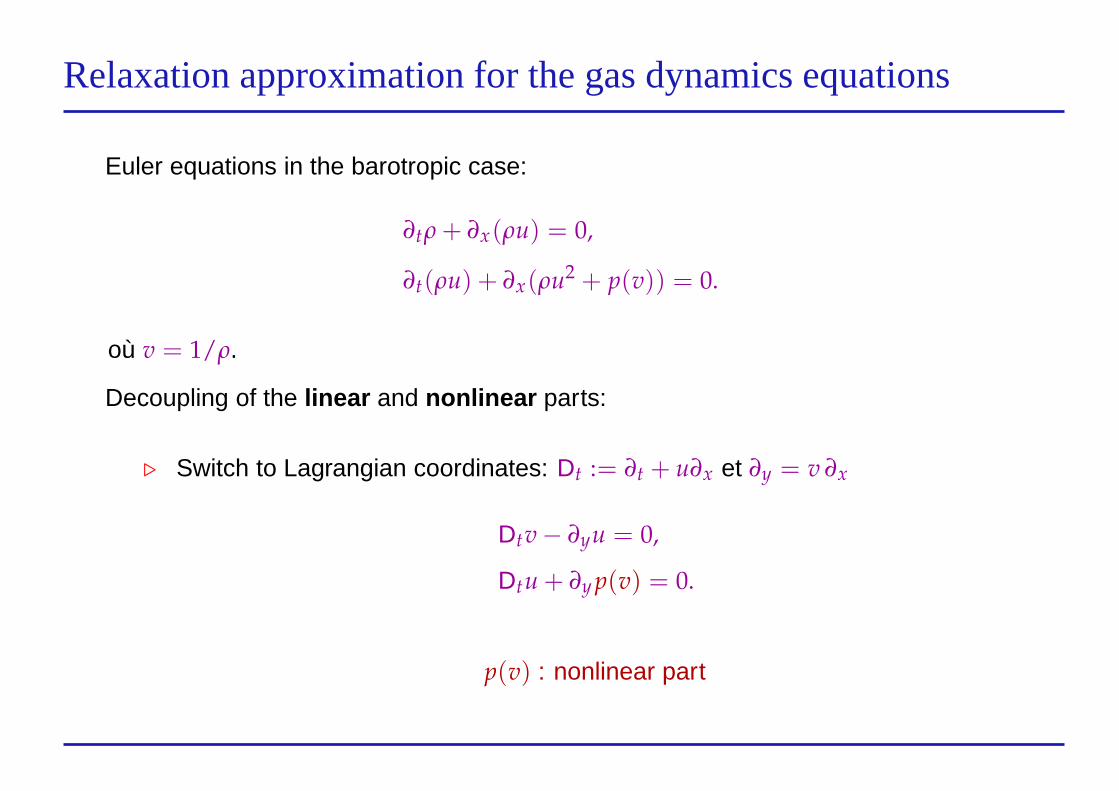
Relaxation approximation for the gas dynamics equations
Euler equations in the barotropic case:
∂tρ + ∂x(ρu) = 0,
∂t(ρu) + ∂x(ρu2 + p(v)) = 0.
où v = 1/ρ.
Decoupling of the linear and nonlinear parts:
⊲ Switch to Lagrangian coordinates: Dt := ∂t + u∂x et ∂y = v ∂x
Dtv− ∂yu = 0,
Dtu + ∂y p(v) = 0.
p(v) : nonlinear part
Relaxation approximation for hyperbolic fluid systems – p. 16/32
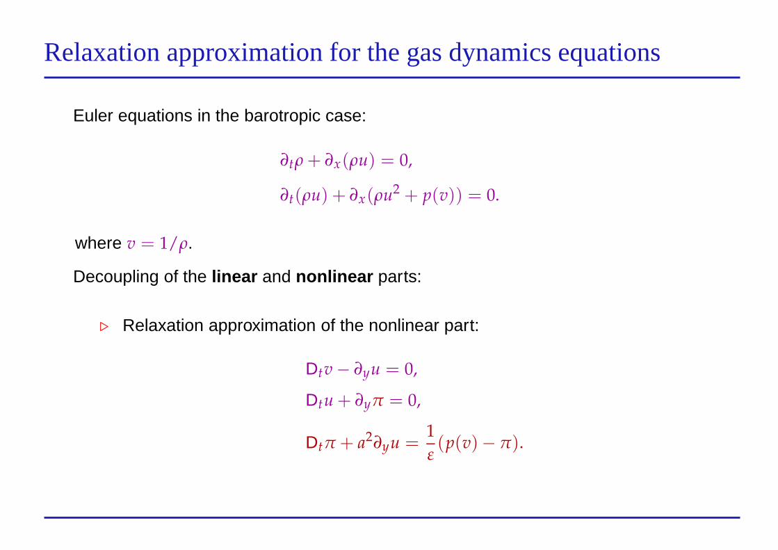
Relaxation approximation for the gas dynamics equations
Euler equations in the barotropic case:
∂tρ + ∂x(ρu) = 0,
∂t(ρu) + ∂x(ρu2 + p(v)) = 0.
where v = 1/ρ.
Decoupling of the linear and nonlinear parts:
⊲ Relaxation approximation of the nonlinear part:
Dtv− ∂yu = 0,
Dtu + ∂yπ = 0,
Dtπ + a2∂yu =1
ε(p(v)− π).
Relaxation approximation for hyperbolic fluid systems – p. 17/32
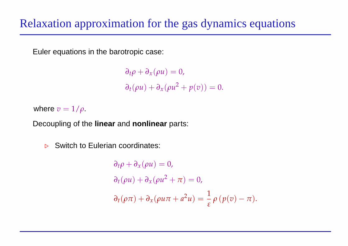
Relaxation approximation for the gas dynamics equations
Euler equations in the barotropic case:
∂tρ + ∂x(ρu) = 0,
∂t(ρu) + ∂x(ρu2 + p(v)) = 0.
where v = 1/ρ.
Decoupling of the linear and nonlinear parts:
⊲ Switch to Eulerian coordinates:
∂tρ + ∂x(ρu) = 0,
∂t(ρu) + ∂x(ρu2 + π) = 0,
∂t(ρπ) + ∂x(ρuπ + a2u) =1
ερ (p(v)− π).
Relaxation approximation for hyperbolic fluid systems – p. 18/32
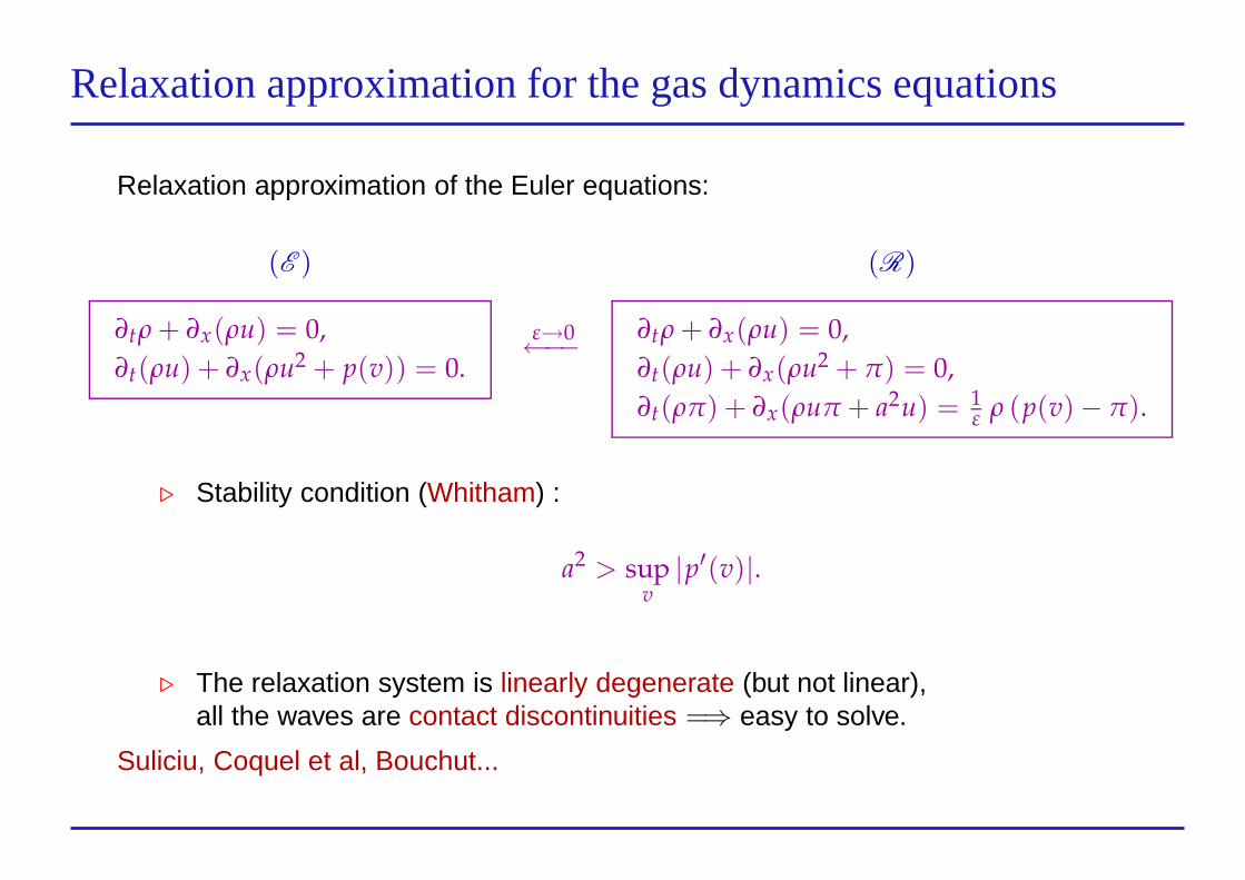
Relaxation approximation for the gas dynamics equations
Relaxation approximation of the Euler equations:
(E )
∂tρ + ∂x(ρu) = 0,
∂t(ρu) + ∂x(ρu2 + p(v)) = 0.
ε→0←−−
(R)
∂tρ + ∂x(ρu) = 0,
∂t(ρu) + ∂x(ρu2 + π) = 0,
∂t(ρπ) + ∂x(ρuπ + a2u) = 1ε ρ (p(v)− π).
⊲ Stability condition (Whitham) :
a2> sup
v|p′(v)|.
⊲ The relaxation system is linearly degenerate (but not linear),all the waves are contact discontinuities =⇒ easy to solve.
Suliciu, Coquel et al, Bouchut...
Relaxation approximation for hyperbolic fluid systems – p. 19/32
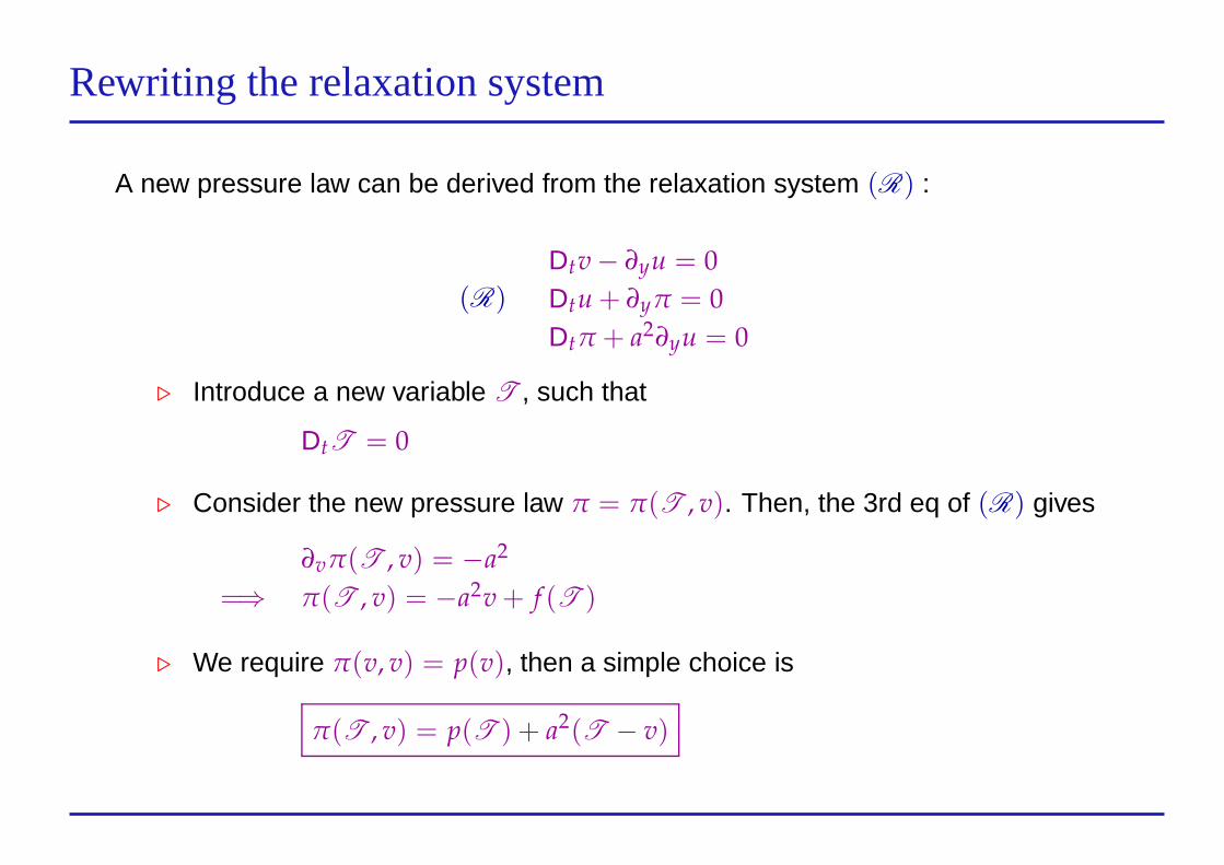
Rewriting the relaxation system
A new pressure law can be derived from the relaxation system (R) :
(R)
Dtv− ∂yu = 0
Dtu + ∂yπ = 0
Dtπ + a2∂yu = 0
⊲ Introduce a new variable T , such that
DtT = 0
⊲ Consider the new pressure law π = π(T , v). Then, the 3rd eq of (R) gives
∂vπ(T , v) = −a2
=⇒ π(T , v) = −a2v + f (T )
⊲ We require π(v, v) = p(v), then a simple choice is
π(T , v) = p(T ) + a2(T − v)
Relaxation approximation for hyperbolic fluid systems – p. 20/32
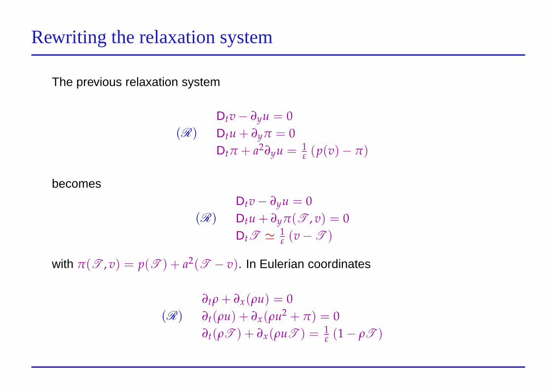
Rewriting the relaxation system
The previous relaxation system
(R)
Dtv− ∂yu = 0
Dtu + ∂yπ = 0
Dtπ + a2∂yu = 1ε (p(v)− π)
becomes
(R)
Dtv− ∂yu = 0
Dtu + ∂yπ(T , v) = 0
DtT ≃1ε (v−T )
with π(T , v) = p(T ) + a2(T − v). In Eulerian coordinates
(R)
∂tρ + ∂x(ρu) = 0
∂t(ρu) + ∂x(ρu2 + π) = 0
∂t(ρT ) + ∂x(ρuT ) = 1ε (1− ρT )
Relaxation approximation for hyperbolic fluid systems – p. 21/32
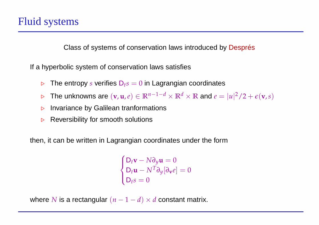
Fluid systems
Class of systems of conservation laws introduced by Després
If a hyperbolic system of conservation laws satisfies
⊲ The entropy s verifies Dts = 0 in Lagrangian coordinates
⊲ The unknowns are (v, u, e) ∈ Rn−1−d ×R
d ×R and e = |u|2/2 + ǫ(v, s)
⊲ Invariance by Galilean tranformations
⊲ Reversibility for smooth solutions
then, it can be written in Lagrangian coordinates under the form
Dtv− N∂yu = 0
Dtu− NT∂y[∂ve] = 0
Dts = 0
where N is a rectangular (n− 1− d)× d constant matrix.
Relaxation approximation for hyperbolic fluid systems – p. 22/32
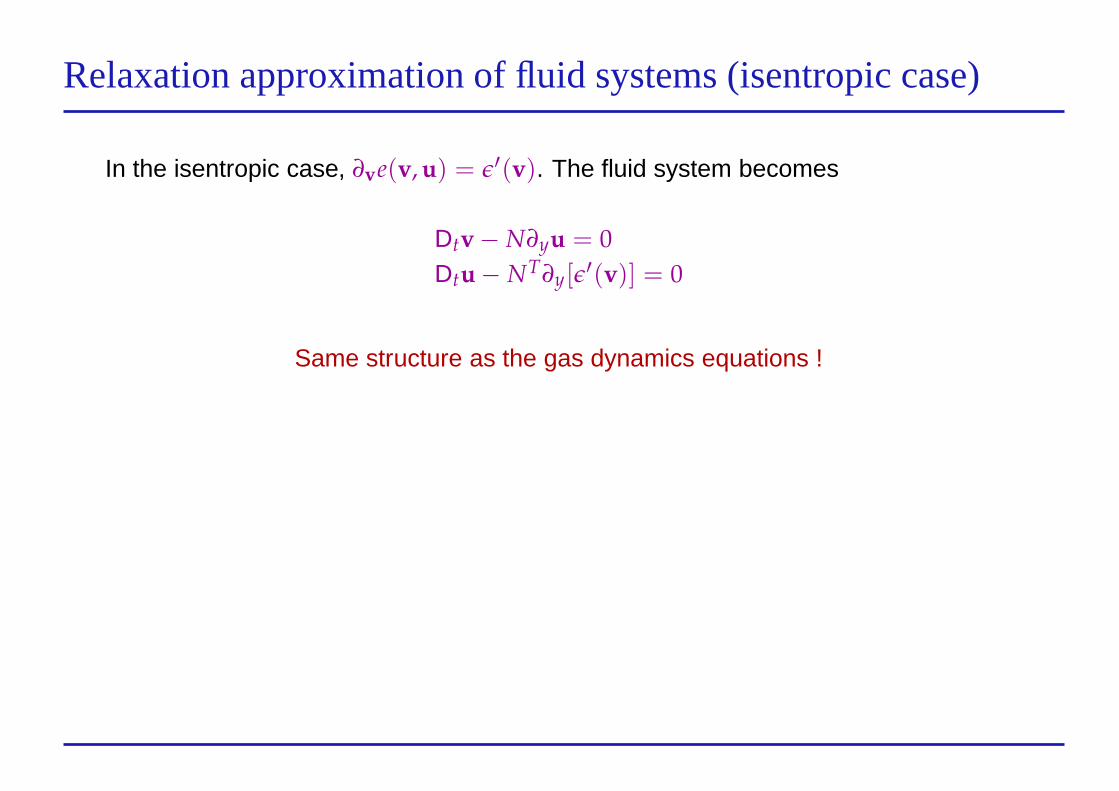
Relaxation approximation of fluid systems (isentropic case)
In the isentropic case, ∂ve(v, u) = ǫ′(v). The fluid system becomes
Dtv− N∂yu = 0
Dtu− NT∂y[ǫ′(v)] = 0
Same structure as the gas dynamics equations !
Relaxation approximation for hyperbolic fluid systems – p. 23/32
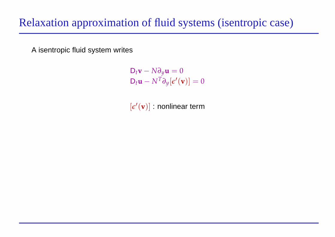
Relaxation approximation of fluid systems (isentropic case)
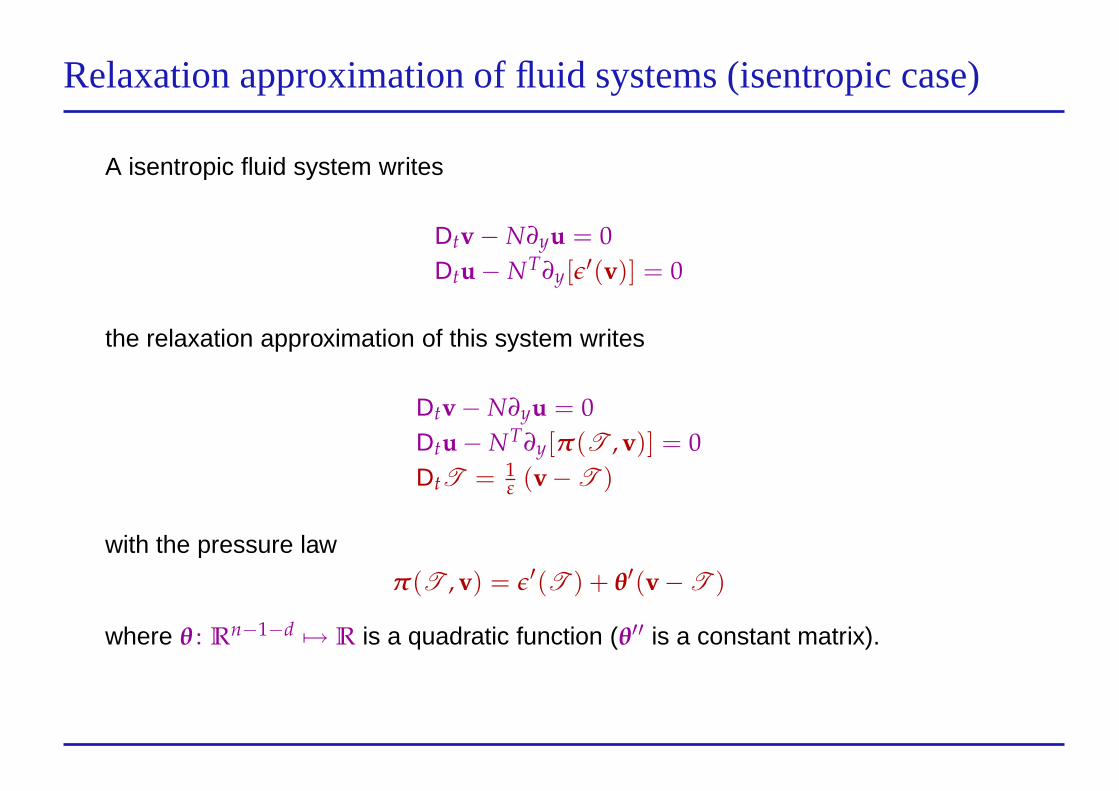
A isentropic fluid system writes
Dtv− N∂yu = 0
Dtu− NT∂y[ǫ′(v)] = 0
[ǫ′(v)] : nonlinear term
Relaxation approximation for hyperbolic fluid systems – p. 24/32
Relaxation approximation of fluid systems (isentropic case)
A isentropic fluid system writes
Dtv− N∂yu = 0
Dtu− NT∂y[ǫ′(v)] = 0
the relaxation approximation of this system writes
Dtv− N∂yu = 0
Dtu− NT∂y[π(T , v)] = 0
DtT = 1ε (v−T )
with the pressure law
π(T , v) = ǫ′(T ) + θ′(v−T )
where θ : Rn−1−d 7→ R is a quadratic function (θ′′ is a constant matrix).
Relaxation approximation for hyperbolic fluid systems – p. 25/32
Relaxation approximation of fluid systems (isentropic case)
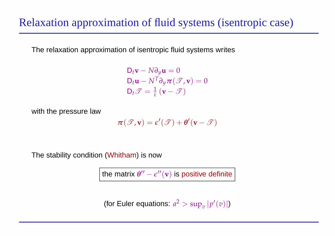
The relaxation approximation of isentropic fluid systems writes
Dtv− N∂yu = 0
Dtu− NT∂yπ(T , v) = 0
DtT = 1ε (v−T )
with the pressure law
π(T , v) = ǫ′(T ) + θ′(v−T )
The stability condition (Whitham) is now
the matrix θ′′ − ǫ′′(v) is positive definite
(for Euler equations: a2> supv |p
′(v)|)
Relaxation approximation for hyperbolic fluid systems – p. 26/32
Relaxation approximation of fluid systems
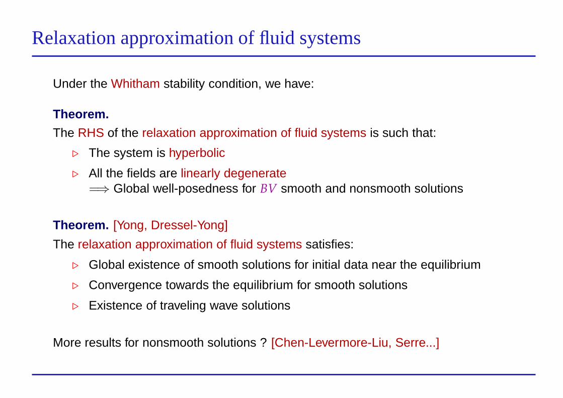
Under the Whitham stability condition, we have:
Theorem.
The RHS of the relaxation approximation of fluid systems is such that:
⊲ The system is hyperbolic
⊲ All the fields are linearly degenerate=⇒ Global well-posedness for BV smooth and nonsmooth solutions
Theorem. [Yong, Dressel-Yong]
The relaxation approximation of fluid systems satisfies:
⊲ Global existence of smooth solutions for initial data near the equilibrium
⊲ Convergence towards the equilibrium for smooth solutions
⊲ Existence of traveling wave solutions
More results for nonsmooth solutions ? [Chen-Levermore-Liu, Serre...]
Relaxation approximation for hyperbolic fluid systems – p. 27/32
Numerical methods
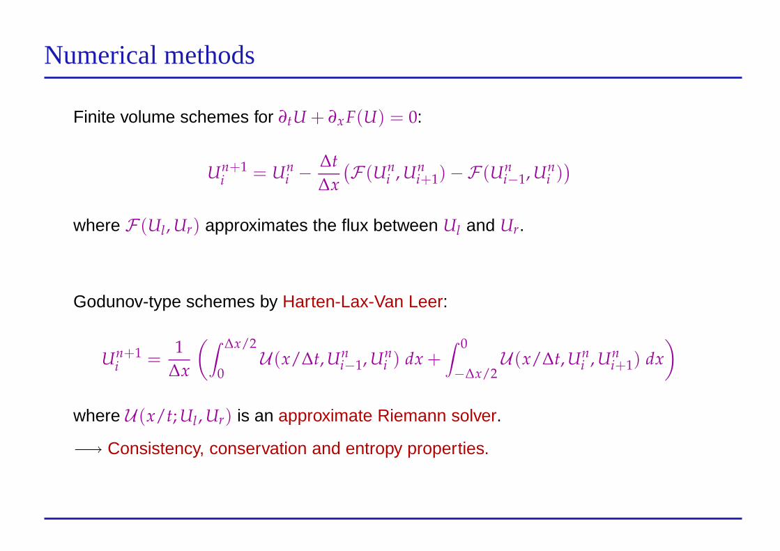
Finite volume schemes for ∂tU + ∂x F(U) = 0:
Un+1i = Un
i −∆t
∆x
(
F (Uni , Un
i+1)−F (Uni−1, Un
i ))
where F (Ul, Ur) approximates the flux between Ul and Ur.
Godunov-type schemes by Harten-Lax-Van Leer:
Un+1i =
1
∆x
(
∫
∆x/2
0U (x/∆t, Un
i−1, Uni ) dx +
∫ 0
−∆x/2U (x/∆t, Un
i , Uni+1) dx
)
where U (x/t; Ul , Ur) is an approximate Riemann solver.
−→ Consistency, conservation and entropy properties.
Relaxation approximation for hyperbolic fluid systems – p. 28/32
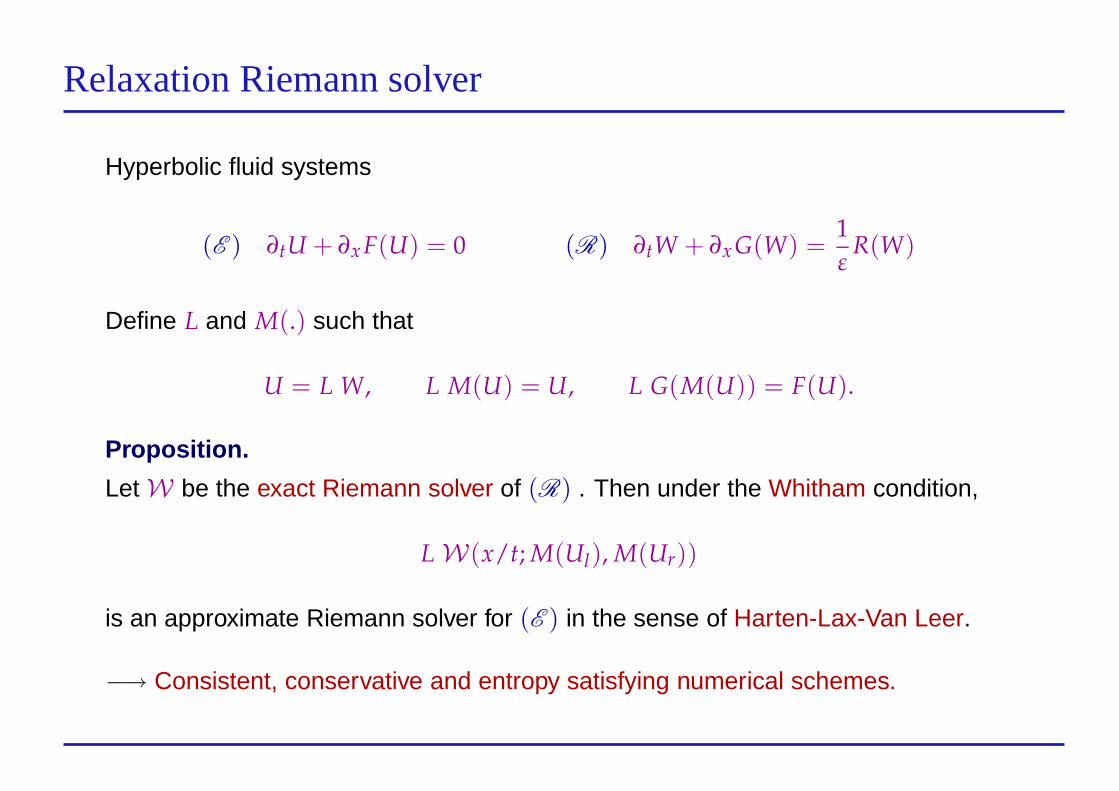
Relaxation Riemann solver
Hyperbolic fluid systems
(E ) ∂tU + ∂x F(U) = 0 (R) ∂tW + ∂xG(W) =1
εR(W)
Define L and M(.) such that
U = L W, L M(U) = U, L G(M(U)) = F(U).
Proposition.
LetW be the exact Riemann solver of (R) . Then under the Whitham condition,
LW(x/t; M(Ul), M(Ur))
is an approximate Riemann solver for (E ) in the sense of Harten-Lax-Van Leer.
−→ Consistent, conservative and entropy satisfying numerical schemes.
Relaxation approximation for hyperbolic fluid systems – p. 29/32
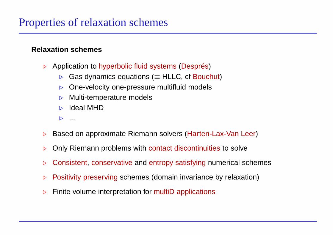
Properties of relaxation schemes
Relaxation schemes
⊲ Application to hyperbolic fluid systems (Després)⊲ Gas dynamics equations (≡ HLLC, cf Bouchut)⊲ One-velocity one-pressure multifluid models⊲ Multi-temperature models⊲ Ideal MHD⊲ ...
⊲ Based on approximate Riemann solvers (Harten-Lax-Van Leer)
⊲ Only Riemann problems with contact discontinuities to solve
⊲ Consistent, conservative and entropy satisfying numerical schemes
⊲ Positivity preserving schemes (domain invariance by relaxation)
⊲ Finite volume interpretation for multiD applications
Relaxation approximation for hyperbolic fluid systems – p. 30/32
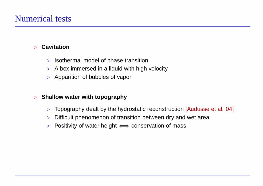
Numerical tests
⊲ Cavitation
⊲ Isothermal model of phase transition⊲ A box immersed in a liquid with high velocity⊲ Apparition of bubbles of vapor
⊲ Shallow water with topography
⊲ Topography dealt by the hydrostatic reconstruction [Audusse et al. 04]⊲ Difficult phenomenon of transition between dry and wet area⊲ Positivity of water height⇐⇒ conservation of mass
Relaxation approximation for hyperbolic fluid systems – p. 31/32
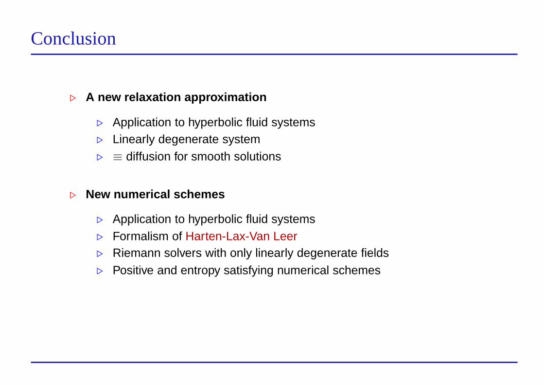
Conclusion
⊲ A new relaxation approximation
⊲ Application to hyperbolic fluid systems⊲ Linearly degenerate system⊲ ≡ diffusion for smooth solutions
⊲ New numerical schemes
⊲ Application to hyperbolic fluid systems⊲ Formalism of Harten-Lax-Van Leer⊲ Riemann solvers with only linearly degenerate fields⊲ Positive and entropy satisfying numerical schemes
Relaxation approximation for hyperbolic fluid systems – p. 32/32
![NON{REPRESENTABLE HYPERBOLIC MATROIDSnamini/PaperA.pdf · and independence polynomials, see [1], Conjecture2.4is true for the rst derivative relaxation of the positive semi-de nite](https://img.pdfslide.us/doc/110x75/5fbe9ff879a0bc64e2095d60/nonrepresentable-hyperbolic-matroids-naminipaperapdf-and-independence-polynomials.jpg)
![I.Theory of the relaxation by collision of molecular ... · 528 approximation is likely to be much more valid for relaxation of polarization than for transfers. In paper II [9], we](https://img.pdfslide.us/doc/110x75/5ecce340bf1a837d176a4a54/itheory-of-the-relaxation-by-collision-of-molecular-528-approximation-is-likely.jpg)


![AN ACCURATE LEGENDRE COLLOCATION SCHEME FOR … · 2 Accurate Legendre collocation scheme for coupled hyperbolic equations 409 [27–29] and function approximation and variational](https://img.pdfslide.us/doc/110x75/5ec5ccd5fe35f6435831c612/an-accurate-legendre-collocation-scheme-for-2-accurate-legendre-collocation-scheme.jpg)