Embed Size (px)
Citation preview
Relative Upper Confidence Bound for theK-Armed Dueling Bandit Problem
Masrour Zoghi1, Shimon Whiteson1 {M.ZOGHI, S.A.WHITESON}@UVA.NLRemi Munos2 [email protected] de Rijke1 [email protected], University of Amsterdam, Netherlands2INRIA Lille - Nord Europe / MSR-NE
AbstractThis paper proposes a new method for the K-armed dueling bandit problem, a variation on theregular K-armed bandit problem that offers onlyrelative feedback about pairs of arms. Our ap-proach extends the Upper Confidence Bound al-gorithm to the relative setting by using estimatesof the pairwise probabilities to select a promisingarm and applying Upper Confidence Bound withthe winner as a benchmark. We prove a sharpfinite-time regret bound of order O(K log T ) ona very general class of dueling bandit problemsthat matches a lower bound proven in (Yue et al.,2012). In addition, our empirical results usingreal data from an information retrieval applica-tion show that it greatly outperforms the state ofthe art.
1. IntroductionIn this paper, we propose and analyze a new algorithm,called Relative Upper Confidence Bound (RUCB), for theK-armed dueling bandit problem (Yue et al., 2012), a vari-ation on the K-armed bandit problem in which the feed-back comes in the form of pairwise preferences. We assessthe performance of this algorithm using one of the maincurrent applications of the K-armed dueling bandit prob-lem, ranker evaluation (Joachims, 2002; Yue & Joachims,2011; Hofmann et al., 2013b), which is used in informationretrieval, ad placement and recommender systems, amongothers.
The K-armed dueling bandit problem is part of thegeneral framework of preference learning (Furnkranz &Hullermeier, 2010), where the goal is to learn, not fromreal-valued feedback, but from relative feedback, which
Proceedings of the 31 st International Conference on MachineLearning, Beijing, China, 2014. JMLR: W&CP volume 32. Copy-right 2014 by the author(s).
specifies only which of two alternatives is preferred. Devel-oping effective preference learning methods is importantfor dealing with domains in which feedback is much morereliable if given in the form of a comparison (e.g., whenprovided by a human) and specifying real-valued feedbackinstead would be arbitrary or inefficient.
Other algorithms proposed for this problem are InterleavedFilter (IF) (Yue et al., 2012), Beat the Mean (BTM) (Yue& Joachims, 2011), and SAVAGE (Urvoy et al., 2013). Allof these methods were designed for the finite-horizon set-ting, in which the algorithm requires as input the explo-ration horizon, T , the time by which the algorithm needsto produce the best arm. The algorithm is then judged basedupon either the accuracy of the returned best arm or the re-gret accumulated in the exploration phase.1 All three ofthese algorithms use the exploration horizon to set theirinternal parameters so that, for each T , there is a sepa-rate algorithm IFT , BTMT and SAVAGET . By contrast,RUCB does not require this input, making it more usefulin practice, since a good exploration horizon is often diffi-cult to guess. Nonetheless, RUCB outperforms these algo-rithms in terms of the accuracy and regret metrics used inthe finite-horizon setting.
The main idea of RUCB is to maintain optimistic estimatesof the probabilities of all possible pairwise outcomes, and(1) use these estimates to select a potential champion,which is an arm that has a chance of being the best arm,and (2) select an arm to compare to this potential championby performing regular Upper Confidence Bound (Agrawal,1995) relative to it.
We prove a finite-time high-probability bound ofO(K log T ) on the cumulative regret of RUCB, fromwhich we deduce a bound on the expectation and all highermoments of cumulative regret. These bounds rely onsubstantially less restrictive assumptions on the K-armeddueling bandit problem than IF and BTM and have bettermultiplicative constants than those of SAVAGE. Further-
1These terms are formalized in Section 2.

Relative Upper Confidence Bound
more, our bounds are the first explicitly non-asymptoticresults for the K-armed dueling bandit problem.
More importantly, the main distinction of our result is that itholds for all time-steps. By contrast, given an explorationhorizon T , the results for IF, BTM and SAVAGE boundonly the regret accumulated by IFT , BTMT and SAVAGETin the first T time-steps.
Finally, we evaluate our method empirically using real datafrom an information retrieval application. The results showthat RUCB can learn quickly and effectively and greatlyoutperforms BTM and SAVAGE.
The main contributions of this paper are as follows:
• A novel algorithm for the K-armed dueling bandit prob-lem that is more broadly applicable than existing algo-rithms,
• Regret bounds that make significantly less restrictive as-sumptions than IF and BTM, have better multiplicativeconstants than the results of SAVAGE, apply to all time-steps, and match an existing asymptotic lower bound,
• A novel proof technique that allows us to obtain the firstlogarithmic high probability regret bound for a UCB-type algorithm that does not require the probability offailure to be passed to the algorithm as a parameter: asa corollary, we also get the first logarithmic bounds onall higher moments of the cumulative regret for all times,and
• Experimental results, based on a real-world application,demonstrating the superior performance of our algorithmcompared to existing methods.
2. Problem SettingThe K-armed dueling bandit problem (Yue et al., 2012) isa modification of the K-armed bandit problem (Thomp-son, 1933): the latter considers K arms {a1, . . . , aK} andat each time-step, an arm ai can be pulled, generating a re-ward drawn from an unknown stationary distribution withexpected value µi. The K-armed dueling bandit problemis a variation in which, instead of pulling a single arm, wechoose a pair (ai, aj) and receive one of them as the betterchoice, with the probability of ai being picked equal to anunknown constant pij and that of aj equal to pji = 1−pij .We define the preference matrix P = [pij ], whose ij entryis equal to pij .
In this paper, we assume that there exists a Condorcet win-ner (Urvoy et al., 2013): an arm, which without loss of gen-erality we label a1, such that p1i >
12 for all i > 1. Given
a Condorcet winner, we define regret for each time-step asfollows (Yue et al., 2012): if arms ai and aj were chosenfor comparison at time t, then regret at that time is rt :=
∆i+∆j
2 , with ∆k := p1k− 12 for all k ∈ {1, . . . ,K}. Thus,
regret measures the average advantage that the Condorcetwinner has over the two arms being compared against eachother. Given our assumption on the probabilities p1k, thisimplies that r = 0 if and only if the best arm is comparedagainst itself. We define cumulative regret up to time T tobe RT :=
∑Tt=1 rt.
The goal of a bandit algorithm can be formalized in severalways. We consider two standard settings:1. The finite-horizon setting, in which the algorithm is told
in advance the exploration horizon, T , i.e., the num-ber of time-steps that the evaluation process is givento explore before it has to produce a single arm as thebest, which will be exploited thenceforth. In this set-ting, the algorithm can be assessed on its accuracy, theprobability that a given run of the algorithm reports theCondorcet winner as the best arm (Urvoy et al., 2013),which is related to expected simple regret: the regret as-sociated with the algorithm’s choice of the best arm, i.e.,rT+1 (Bubeck et al., 2009). Another measure of successin this setting is the amount of regret accumulated dur-ing the exploration phase, as used in the explore-then-exploit problem formulation (Yue et al., 2012).
2. The horizonless setting, in which no horizon is spec-ified and the evaluation process continues indefinitely.Thus, it is no longer sufficient for the algorithm to max-imize accuracy or minimize regret after a single horizonis reached. Instead, it must minimize regret across allhorizons by rapidly decreasing the frequency of com-parisons involving suboptimal arms, particularly thosethat fare worse in comparison to the best arm. This goalcan be formulated as minimizing the cumulative regretover time, rather than with respect to a fixed horizon(Lai & Robbins, 1985).
All existing K-armed dueling bandit methods target thefinite-horizon setting. However, we argue that the horizon-less setting is more relevant in practice for the followingreason: finite-horizon methods require a horizon as inputand often behave differently for different horizons. Thisposes a practical problem because it is typically difficultto know in advance how many comparisons are requiredto determine the best arm with confidence and thus howto set the horizon. If the horizon is set too long, the al-gorithm is too exploratory, increasing the number of eval-uations needed to find the best arm. If it is set too short,the best arm remains unknown when the horizon is reachedand the algorithm must be restarted with a longer horizon.
Moreover, any algorithm that can deal with the horizonlesssetting can easily be modified to address the finite-horizonsetting by simply stopping the algorithm when it reachesthe horizon and returning the best arm. By contrast, forthe reverse direction, one would have to resort to the “dou-

Relative Upper Confidence Bound
bling trick” (Cesa-Bianchi & Lugosi, 2006, Section 2.3),which leads to substantially worse regret results: this isbecause all of the upper bounds proven for methods ad-dressing the finite-horizon setting so far are in O(log T )and applying the doubling trick to such results would leadto regret bounds of order (log T )2, with the extra log factorcoming from the number of partitions.
To the best of our knowledge, RUCB is the first K-armeddueling bandit algorithm that can function in the horizon-less setting without resorting to the doubling trick. Weshow in Section 4 how it can be adapted to the finite-horizon setting.
3. Related WorkThe first two methods proposed for the K-armed duelingbandit problem are Interleaved Filter (IF) (Yue et al., 2012)and Beat the Mean (BTM) (Yue & Joachims, 2011), bothof which were designed for a finite-horizon scenario. Thesemethods work under the following restrictions: a total or-dering of the arms, Stochastic Triangle Inequality (STI) andeither Strong Stochastic Transitivity (SST) in the case ofIF or Relaxed Stochastic Transitivity (RST) with parame-ter γ (for BTM); γ, which measures the degree to whichSST fails to hold, needs to be passed to the algorithm: thehigher γ is, the more challenging the problem becomes,with SST holding when γ = 1 (cf. §8.1 of the supplemen-tary material for formal definitions and evidence that theseassumptions are often violated in practice).
Given these assumptions, the following regret bounds havebeen proven for IF and BTM. For large T we have
E[RIFTT
]≤ CK log T
∆min, and
RBTMTT ≤ C ′ γ
7K log T
∆minwith high probability,
where IFT means that IF is run with the exploration horizonset to T and similarly for BTMT ; ∆min is the smallest gap∆j := p1j − 1
2 , assuming that a1 is the best arm; and Cand C
′are universal constants that do not depend on the
specific dueling bandit problem.
The first bound holds only when γ = 1 but matches thelower bound in (Yue et al., 2012, Theorem 2). The secondbound holds for γ ≥ 1 and is sharp when γ = 1. Note thatthis lower bound was proven for certain K-armed duelingbandit problems that satisfy ∆i = ∆j for all i, j 6= 1. Inthis case, our asymptotic regret bound matches this lowerbound as well, without any dependence on γ (cf. Theorem4).
Sensitivity Analysis of VAriables for Generic Exploration(SAVAGE) (Urvoy et al., 2013) is a recently proposed al-gorithm that outperforms both IF and BTM by a wide mar-
gin when the number of arms is of moderate size. More-over, one version of SAVAGE, called Condorcet SAVAGE,makes the Condorcet assumption and has the best theo-retical results among the algorithms studied in that pa-per (Urvoy et al., 2013, Theorem 3). However, the regretbounds provided for Condorcet SAVAGE are of the formO(K2 log T ), and so are not as tight as those of IF, BTMor our algorithm.
Finally, note that all of the above results bound only RT ,where T is the predetermined horizon, since IF, BTM andSAVAGE were designed for the finite-horizon setting. Bycontrast, in Section 5, we bound the cumulative regret ofRUCB for all time-steps.
4. Method
Algorithm 1 Relative Upper Confidence BoundInput: α > 1
2 , T ∈ {1, 2, . . .} ∪ {∞}1: W = [wij ] ← 0K×K // 2D array of wins: wij is the
number of times ai beat aj2: B = ∅3: for t = 1, . . . , T do4: U := [uij ] = W
W+WT +√
α ln tW+WT // All opera-
tions are element-wise; x0 := 1 for any x.5: uii ← 1
2 for each i = 1, . . . ,K.6: C ←
{ac | ∀ j : ucj ≥ 1
2
}.
7: If C = ∅, then pick c randomly from {1, . . . ,K}.8: B ← B ∩ C.9: If |C| = 1, then B ← C and ac to be the unique
element in C.10: if |C| > 1 then11: Sample ac from C using the distribution:
p(ac) =
{0.5 if ac ∈ B,
1
2|B| |C\B|
otherwise.12: end if13: d ← arg maxj ujc, with ties broken randomly.
Moreover, if there is a tie, d is not allowed to beequal to c.
14: Compare arms ac and ad and increment wcd or wdcdepending on which arm wins.
15: end forReturn: An arm ac that beats the most arms, i.e., c with
the largest count #{j| wcjwcj+wjc
> 12
}.
We now introduce Relative Upper Confidence Bound(RUCB), which is applicable to any K-armed dueling ban-dit problem with a Condorcet winner. In each time-step,RUCB, shown in Algorithm 1, goes through the followingthree stages:
(1) RUCB puts all arms in a pool of potential champions.Then, it compares each arm ai against all other arms op-

Relative Upper Confidence Bound
timistically: for all i 6= j, it computes the upper bounduij(t) = µij(t) + cij(t), where µij(t) is the frequentist es-timate of pij at time t and cij(t) is an optimism bonus thatincreases with t and decreases with the number of compar-isons between i and j (Line 4). If uij < 1
2 for any j, thenai is removed from the pool: the set of remaining arms iscalled C. If we are left with a single potential championat the end of this process, we let ac be that arm and put itin the set B of the hypothesized best arm (Line 9). Notethat B is always either empty or contains one arm; more-over, an arm is demoted from its status as the hypothesizedbest arm as soon as it optimistically loses to another arm(Line 8). Next, from the remaining potential champions,a champion arm ac is chosen in one of two ways: if B isempty, we sample an arm from C uniformly randomly; if Bis non-empty, the probability of picking the arm in B is setto 1
2 and the remaining arms are given equal probability ofbeing chosen (Line 11).
(2) Regular UCB is performed using ac as a bench-mark (Line 13), i.e., UCB is performed on the set ofarms a1c . . . aKc. Specifically, we select the arm d =arg maxj ujc. When c 6= j, ujc is defined as above. Whenc = j, since pcc = 1
2 , we set ucc = 12 (Line 5).
(3) The pair (ac, ad) is compared and the score sheet isupdated as appropriate (Line 7).
Note that in stage (1) the comparisons are based on ucj ,i.e., ac is compared optimistically to the other arms, mak-ing it easier for it to become the champion. By contrast,in stage (2) the comparisons are based on ujc, i.e., ac iscompared to the other arms pessimistically, making it moredifficult for ac to be compared against itself. This is impor-tant because comparing an arm against itself yields no in-formation. Thus, RUCB strives to avoid auto-comparisonsuntil there is great certainty that ac is indeed the Condorcetwinner.
Eventually, as more comparisons are conducted, the esti-mates µ1j tend to concentrate above 1
2 and the optimismbonuses c1j(t) become small. Thus, both stages of the al-gorithm increasingly select a1, i.e., ac = ad = a1, whichaccumulates zero regret.
Note that Algorithm 1 is a finite-horizon algorithm if T <∞ and a horizonless one if T = ∞, in which case the forloop never terminates.
5. Theoretical ResultsIn this section, we prove finite-time high-probability andexpected regret bounds for RUCB. We first state Lemma 1and use it to prove a high-probability bound on the numberof comparisons for each suboptimal arm in Proposition 2.An immediate consequence of this result is a high probabil-
ity regret bound of the form O(K2 log T ), which is similarto the bound for SAVAGE (Urvoy et al., 2013) but for thehorizonless setting. However, in Theorem 4 we show thatthis can be lowered to O(K log T ) and we deduce an ex-pected regret bound in Theorem 5. This result is provenunder conditions that are much more general than those forIF (Yue et al., 2012) and without requiring the user to spec-ify the γ parameter as BTM does (Yue & Joachims, 2011).Moreover, it matches the asymptotic lower bound provenin (Yue et al., 2012, Theorem 2).
The results in Theorems 4 and 5 are surprising because aK-armed dueling bandit problem depends on roughly K2
2independent parameters, so one would expect a bound ofthe form O(K2 log T ) unless strong prior information isinfused into the algorithm, as with IF and BTM. However,these theorems show that one can get asymptotic behaviourresembling that of a regular K-armed bandit algorithm ona very broad class of dueling bandit problems with verylittle prior knowledge. This finding is also of great practi-cal significance because there are many situations in whichone has a choice between applying a K-armed bandit al-gorithm to an unreliable quantity, such as Click ThroughRate, or using a K-armed dueling bandit algorithm to con-duct direct comparisons, which are known to be more re-liable when dealing with humans (Hofmann et al., 2013a,§2.1). These results show that, given such a dilemma, usinga dueling bandit approach does not come at the expense ofthe asymptotic behaviour.
Finally, note that the high probability bound proven in The-orem 4 does not rely on the probability of failure, δ, beingpassed to the algorithm. Thus, we can use it to also boundhigher moments (hence also the variance) of the cumulativeregret for RUCB for all times. This is in contrast to highprobability bounds that require δ to be specified before thealgorithm starts (Audibert et al., 2009; Srinivas et al., 2010;Abbasi-yadkori et al., 2011), from which one cannot obtainexpected regret bounds for all times. While, given a timeT , one can set δ = 1/T in the algorithm to get a logarith-mic expected regret bound at time T , getting a logarithmicexpected regret bound at time T 1+ε for any ε > 0, requiresrerunning the algorithm with δ = 1/T 1+ε.
As before, we assume without loss of generality that a1 isthe optimal arm. See Table 1 for definitions of symbolsused throughout.
Lemma 1. Let P := [pij ] be the preference matrix of aK-armed dueling bandit problem with arms {a1, . . . , aK}.Then, for any dueling bandit algorithm and any α > 1
2 andδ > 0, we have
P(∀ t > C(δ), i, j, pij ∈ [lij(t), uij(t)]
)> 1− δ.
Proof. See §8.2 in the supplementary material.
Relative Upper Confidence Bound
Table 1. List of notation used in this sectionSymbol Definition
K Number of armsα The input of Algorithm 1Nij(t) Number of comparisons between ai and aj until time
twij(t) Number of wins of ai over aj until time t
uij(t)wij(t)
Nij(t)+
√α ln t
Nij(t)lij(t) 1− uji(t)δ Probability of failure
C(δ)
((4α− 1)K2
(2α− 1)δ
) 12α−1
∆j p1j − 0.5
∆ij∆i + ∆j
2∆max maxi ∆i
Dij4α
min{∆2i ,∆
2j}
, or4α
∆2j
if i = 1, or 0 if i = j
D∑i<j
Dij
C(δ)
(4∆max log
2
δ+ 2∆maxC
(δ
2
)+ 2D ln 2D
)Dj
2α (∆j + 4∆max)
∆2j
Tδ Definition 3Tδ A time between C(δ/2) and Tδ when a1 was com-
pared against itselfa ∨ b max{a, b}
Let us now turn to our first high-probability bound:
Proposition 2. Given K arms {a1, . . . , aK} with prefer-ence matrix P = [pij ], such that a1 is the Condorcet win-ner, and δ > 0 and α > 1
2 , then, if we apply Algorithm1 to this K-armed dueling bandit problem, given any pair(i, j) 6= (1, 1), the number of comparisons between armsai and aj performed up to time t, denoted by Nij(t), satis-fies
P(∃ t, (i, j) 6= (1, 1): Nij(t) > C(δ)∨Dij ln t
)< δ (1)
and, Nδij(t), the number of times ai was compared against
aj between time-steps C(δ) and t, satisfies
P(∃ t > C(δ), (i, j) 6= (1, 1): Nδ
ij(t) > Dij ln t)< δ (2)
Proof. Given Lemma 1, we know with probability 1 − δthat pij ∈ [lij(t), uij(t)] for all t > C(δ). Let us first dealwith the easy case when i = j 6= 1: when t > C(δ) holds,ai cannot be played against itself, since if we get c = i inAlgorithm 1, then by Lemma 1 and the fact that a1 is theCondorcet winner we have d 6= i since uii(t) = 1
2 < p1i ≤u1i(t).
Now, let us assume that distinct arms ai and aj have beencompared against each other more than Dij ln t times andthat t > C(δ). If s is the last time ai and aj were comparedagainst each other, we must have
a1
12
a1
ai aj
12
pi1
ai∆i
12
pj1
aj∆j
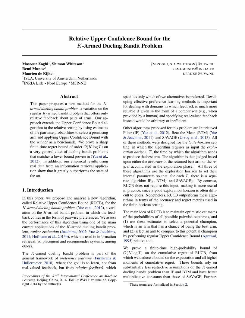
Figure 1. An illustration of the proof of Proposition 2. The figureshows an example of the internal state of RUCB at time s. Theheight of the dot in the block in row am and column an repre-sents the comparisons probability pmn, while the interval, wherepresent, represents the confidence interval [lmn, umn]: we haveonly included them in the (ai, aj) and the (aj , ai) blocks of thefigure because those are the ones that are discussed in the proof.Moreover, in those blocks, we have included the outcomes of twodifferent runs: one drawn to the left of the dots representing pijand pji, and the other to the right (the horizontal axis in these plotshas no other significance). These two outcomes are included toaddress the dichotomy present in the proof. Note that for a givenrun, we must have [lji(s), uji(s)] = [1 − uij(s), 1 − lij(s)] forany time s, hence the symmetry present in this figure.
uij(s)− lij(s) = 2
√α ln s
Nij(t)(3)
≤ 2
√α ln t
Nij(t)< 2
√√√√ α ln t4α ln t
min{∆2i ,∆
2j}
= min{∆i,∆j}.
On the other hand, for ai to have been compared againstaj at time s, one of the following two scenarios must havehappened:
I. In Algorithm 1, we had c = i and d = j, in whichcase both of the following inequalities must hold:a. uij(s) ≥ 1
2 , since otherwise c could not have beenset to i by Line 5 of Algorithm 1, and
b. lij(s) = 1 − uji(s) ≤ 1 − p1i = pi1, since weknow that p1i ≤ u1i(t), by Lemma 1 and the factthat t > C(δ), and for d = j to be satisfied, wemust have u1i(t) ≤ uji(t) by Line 6 of Algorithm1.
From these two inequalities, we can conclude
uij(s)− lij(s) ≥1
2− pi1 = ∆i. (4)
Relative Upper Confidence Bound
This inequality is illustrated using the lower rightconfidence interval in the (ai, aj) block of Figure 1,where the interval shows [lij(s), uij(s)] and the dis-tance between the dotted lines is 1
2 − pi1.
II. In Algorithm 1, we had c = j and d = i, in whichcase swapping i and j in the above argument gives
uji(s)− lji(s) ≥1
2− pj1 = ∆j . (5)
Similarly, this is illustrated using the lower left confi-dence interval in the (aj , ai) block of Figure 1, wherethe interval shows [lji(s), uji(s)] and the distance be-tween the dotted lines is 1
2 − pj1.
Putting (4) and (5) together with (3) yields a contradiction,so with probability 1−δ we cannot haveNij be larger thanboth C(δ) and Dij ln t. This gives us both (1) and (2).
We use the next definition in what follows:
Definition 3. Let Tδ be the smallest time satisfying
Tδ > C
(δ
2
)+∑
i<j
Dij ln Tδ,
which is guaranteed to exist since the expression on the leftof the inequality grows linearly with Tδ and the expressionon the right grows logarithmically. Note that Tδ is specifiedby the K-armed dueling bandit problem.
With this in hand, we now state our main result:
Theorem 4. Given the setup of Proposition 2, for any δ >0, we have with probability 1 − δ that for all times T thefollowing bound on the cumulative regret holds:
RT ≤ C(δ) +
K∑
j=2
Dj lnT, (6)
where
C(δ) :=
(4 ln
2
δ+ 2C
(δ
2
)+ 2D ln 2D
)∆max
Dj := D1j (∆1j + 2∆max) =2α (∆j + 4∆max)
∆2j
,
with C(·) and D as in Proposition 2, and ∆max:=maxi ∆i
and ∆ij :=∆i+∆j
2 , while RT is the cumulative regret asdefined in Section 2.
Proof. If we apply Inequality (2) in Proposition 2 witht = Tδ (as in Definition 3), we know that with prob-ability 1 − δ
2 there is a time Tδ ∈(C(δ2
), Tδ
]when
arm a1 was compared against itself, which means that atthat time we had uj1(Tδ) <
12 . This in turn implies that
B = {a1} from that point on, since by Lemma 1 we havethat 1
2 < p1j ≤ u1j(t) for all t > Tδ > C(δ2
).
Since we have B = {a1}, we know that when choosingac in Algorithm 1, the probability of choosing a1 is equalto 1
2 . Given this, we can expect that from Tδ onwards, thealgorithm will spend roughly half of its time comparing a1
against other arms. In what follows, we show that this isindeed the case.
Let Nij(T ) denote the number of times arm ai was com-pared against aj between times Tδ and T . Proposition 2shows that, again with probability 1− δ
2 , we have Nij(T ) ≤Dij lnT for all i < j: note that this 1 − δ
2 is the same asthe one used above. In particular, this means that N1(T ),the number of times between times Tδ and T when we hadc = 1 6= d, is bounded by
N1(T ) ≤K∑
j=2
N1j(T ) ≤K∑
j=2
D1j lnT =: N1(T ). (7)
Let us introduce here two sets of random variables:
• τ0, τ1, τ2, . . ., where τ0 := Tδ and τl is the lth time arma1 was compared against another arm after Tδ .
• n1, n2, . . ., where nl is the number of times in Algorithm1 we had c 6= 1 6= d between τl−1 and τl.
Now, note that RUCB chooses c 6= 1 or d 6= 1 in time-stept if and only if uj1(t) ≥ 1
2 for some j > 1 and that we canhave uj1(t+ 1) < uj1(t) only if at the end of the tth itera-tion, arm a1 was compared against arm aj . In other words,whenever we have uj1(T ) ≥ 1
2 for some j > 1, the algo-rithm will continue to set (c, d) 6= (1, 1) until all of the uj1with j > 1 get submerged below 1
2 and that the last com-parison before we get to this state must be between a1 andanother arm. With this picture in mind, with probability1− δ
2 , we have
RT ≤ Tδ∆max +
K∑
j=2
D1j∆1j lnT +
N1(T )∑
l=1
nl∆max, (8)
where N1(T ) is as in Inequality (7), and so all we needto do is bound Tδ and the sum of the intervals nl for l =1, . . . , N1(T ). Let us deal with the former first: we knowthat Tδ ≤ Tδ and that the latter is defined to be the smallesttime-step satisfying the inequality in Definition 3, so allwe need to do is produce one number that, when pluggedin for Tδ , satisfies the inequality, and one such number is2C(δ2
)+ 2D ln 2D. To see this, let us temporarily use
the notation C := C(δ2
), and use the concavity of the log
function, a first order Taylor expansion, and the fact that wehave lnx < x for any x, to get
C +D ln(2C + 2D ln 2D)
≤ C +D ln(2D ln 2D) +��D�2C
��2D ln 2D
≤ C +D ln(2D)2 + C = 2C + 2D ln 2D,
where we used the fact that D > 2 and so ln 2D > 1.
Relative Upper Confidence Bound
Let us now return to the task of bounding the sum of theintervals nl. To do so, we introduce the random variablesn1, n2, . . ., which are independent samples from the geo-metric distribution with decay 1
2 . Note that nl bounds nlfrom above since it counts the number of iterations it wouldtake for Line 11 of Algorithm 1 to produce a1 and oncewe have c = 1, we are guaranteed to have a comparisonbetween a1 and another arm, as long as uj1 ≥ 1
2 for somej > 1. Furthermore, the sum of independent geometric ran-dom variables has a negative binomial distribution (Feller,1968, §VI.8), with the following probability mass function,cf. (Feller, 1968, Equation VI.8.1):
f(n; r) := P
(r∑
l=1
nl = n
)=
(n+r−1n
)
2n+r,
where in our case p = 12 and so it is eliminated from the
notation of the PMF. In order to bound this sum with highprobability, we note that when n ≥ 2r, then we have
f(n; r)
f(n+ 1; r)=
(n+r−1n
)
2n+r(n+rn+1
)
2n+r+1
=
(n+ r − 1)!
n!(r − 1)!
(n+ r)!
(n+ 1)!(r − 1)!× 2
=2(n+ 1)
n+ r= 2
[1− r − 1
n+ r
]≥ 2− 2r − 2
3r>
4
3.
Thus, we have f(n; r) ≤ f(2r; r)(
34
)n−2r ≤(
34
)n−2rfor
all n ≥ 2r, since f(2r; r) is a probability and so at mostequal to 1. From this we can conclude that with probability
1− δ2 , we have n ≤ 2r+
ln δ2
ln 34
< 2r−4 ln δ2 : note that both
the numerator and the denominator of the second summandare negative and so the fraction is positive. Now, settingr = N1(T ) :=
∑Kj=2D1j lnT and plugging the resulting
upper bound into the regret bound given in (8) give us thedesired result.
Next, we state our expected regret bound, which is a directconsequence of Theorem 4:
Theorem 5. Given the setup of Proposition 2 together withthe notation of Theorem 4, we have the following expectedregret bound for RUCB, where the expectations are takenacross different runs of the algorithm: if we have α > 1, theexpected regret accumulated by RUCB after T iterations isbounded by
E[RT ] ≤[
8 +
(2(4α− 1)K2
2α− 1
) 12α−1 2α− 1
α− 1
]∆max
+ 2D∆max ln 2D +
K∑
j=2
2α (∆j + 4∆max)
∆2j
lnT,
Proof. See §8.3 in the supplementary material.
Remark 6. (1) Using a very similar argument as the oneused to prove Theorem 5, we can also bound the mth mo-ment of RT whenever we have α > m+1
2 , which can beused to bound its variance for α > 1.5.
(2) In general, our regret bounds are not directly compa-rable to those of IF and BTM, since those bounds dependonly on ∆min; so, if the majority of the ∆j are larger than∆min, then our upper bound is lower than that of IF andBTM. On the other hand, if most ∆j are close to ∆min, but∆max is much larger, then the upper bound for IF would belower: the same would hold for BTM if γ is small.
(3) Note that RUCB uses the upper-confidence bounds(Line 3 of Algorithm 1) introduced in the original ver-sion of UCB (Auer et al., 2002) (up to the α factor). Re-cently refined upper-confidence bounds (such as UCB-V(Audibert et al., 2009) or KL-UCB (Cappe et al., 2013))have improved performance for the regular K-armed ban-dit problem. However, in our setting the arm distributionsare Bernoulli and the comparison value is 1/2. Thus, sincewe have 2∆2
i ≤ kl(p1,i, 1/2) ≤ 4∆2i (where kl(a, b) =
a ln ab + (1 − a) ln 1−a
1−b is the KL divergence betweenBernoulli distributions with parameters a and b), we de-duce that using KL-UCB instead of UCB does not improvethe leading constant in the logarithmic term of the regret bya numerical factor of more than 2.
6. ExperimentsTo evaluate RUCB, we apply it to the problem ofranker evaluation from the field of information retrieval(IR) (Manning et al., 2008). A ranker is a function thattakes as input a user’s search query and ranks the docu-ments in a collection according to their relevance to thatquery. Ranker evaluation aims to determine which amonga set of rankers performs best. One effective way to achievethis is to use interleaved comparisons (Radlinski et al.,2008), which interleave the documents proposed by twodifferent rankers and presents the resulting list to the user,whose resulting click feedback is used to infer a noisy pref-erence for one of the rankers. Given a set of K rankers, theproblem of finding the best ranker can then be modeled asa K-armed dueling bandit problem, with each arm corre-sponding to a ranker.
We evaluated RUCB, Condorcet SAVAGE and BTM usingrandomly chosen subsets from the pool of 64 rankers pro-vided by LETOR, a standard IR dataset (see §8.4 for moredetails of the experimental setup), yielding K-armed du-eling bandit problems with K ∈ {16, 32, 64}. For eachset of rankers, we performed 100 independent runs of eachalgorithm for a maximum of 4.5 million iterations. ForRUCB we set α = 0.51, which approaches the limit setby our high-probability result. Since BTM and SAVAGE

Relative Upper Confidence Bound
103 104 105 106
time
2000
4000
6000
8000
cum
ulat
ive
regr
etLETOR NP2004 Dataset with 16 rankers
103 104 105 106
time
5000
10000
15000
20000
25000
30000
35000
cum
ulat
ive
regr
et
LETOR NP2004 Dataset with 32 rankers
103 104 105 106
time
20000
40000
60000
80000
100000
120000
140000
cum
ulat
ive
regr
et
LETOR NP2004 Dataset with 64 rankers
BTMCondorcet SAVAGERUCB α = 0.51
Figure 2. Average cumulative regret for 100 runs of BTM, Condorcet SAVAGE and RUCB with α = 0.51 applied to three K-armeddueling bandit problems with K = 16, 32, 64. Note the time axis uses a log scale, so that the curves depict the relation between log Tand RT ; also, the dotted curves signify best and worst regret performances across all runs.
require the exploration horizon as input, we ran BTMT andCSAVAGET for various horizons T ranging from 1000 to4.5 million. In the plots in Figure 2, the markers on thegreen and the blue curves show the regret accumulated byBTMT and CSAVAGET in the first T iteration of the algo-rithm for each of these horizons. Thus, each marker corre-sponds, not to the continuation of the runs that produced theprevious marker, but to new runs conducted with a larger T .
Since RUCB is horizonless, we ran it for 4.5 million iter-ations and plotted the cumulative regret, as shown usingthe red curves in the plots in Figure 2. For all three algo-rithms, the middle curve shows average cumulative regretand the dotted lines show minimum and maximum cumu-lative regret across runs. Note that these plots are in log-linear scale, so they depict the relation between RT andlog T , which can be seen to be asymptotically linear. Theregret curves for BTM are cut-off in these plots, since inall three experiments RBTMT
T grew linearly with T in thefirst 4.5 million iterations. As can be seen from the plots inFigure 2, RUCB accumulates the least regret of the three al-gorithms: the average regret accumulated by RUCB is lessthan half of that Condorcet SAVAGE by the end of each ofthe three experiments and even the worst performing run ofRUCB accumulated considerably less regret than the bestperforming run of Condorcet SAVAGE.
7. ConclusionsThis paper proposed a new method called Relative Up-per Confidence Bound (RUCB) for the K-armed duelingbandit problem that extends the Upper Confidence Bound(UCB) algorithm to the relative setting by using optimisticestimates of the pairwise probabilities to choose a potentialchampion and conducting regular UCB with the championas the benchmark.
We proved finite-time high-probability and expected regretbounds for RUCB that match an existing lower bound. Un-
like existing results, our regret bounds hold for all time-steps, rather than just a specific horizon T input to the algo-rithm. Furthermore, they take the form O(K log T ) whilemaking much less restrictive assumptions than existing al-gorithms with similar bounds. Finally, the empirical re-sults showed that RUCB greatly outperforms state-of-the-art methods.
In future work, we will consider two extensions to this re-search. First, building off extensions of UCB to the con-tinuous bandit setting (Srinivas et al., 2010; Bubeck et al.,2011; Munos, 2011; de Freitas et al., 2012; Valko et al.,2013), we aim to extend RUCB to the continuous duelingbandit setting, without a convexity assumption as in (Yue& Joachims, 2009; Jamieson et al., 2012). Second, build-ing off Thompson Sampling (Thompson, 1933; Agrawal &Goyal, 2012; Kauffmann et al., 2012), an elegant and effec-tive sampling-based alternative to UCB, we will investigatewhether a sampling-based extension to RUCB would beamenable to theoretical analysis. Both these extensions in-volve overcoming not only the technical difficulties presentin the regular bandit setting, but also those that arise fromthe two-stage nature of RUCB. Since the submission of thispaper, the latter of these two ideas has been validated ex-perimentally in (Zoghi et al., 2014), although a theoreticalanalysis is still lacking.
AcknowledgmentsThis research was partially supported by the European Com-munity’s Seventh Framework Programme (FP7/2007-2013) un-der grant agreements nr 270327, nr 288024 and nr 312827, theNetherlands Organisation for Scientific Research (NWO) underproject nrs 727.011.005, 612.001.116, HOR-11-10, 640.006.013,the Center for Creation, Content and Technology (CCCT), theQuaMerdes project funded by the CLARIN-nl program, theTROVe project funded by the CLARIAH program, the Dutch na-tional program COMMIT, the ESF Research Network ProgramELIAS, the Elite Network Shifts project funded by the RoyalDutch Academy of Sciences (KNAW), the Netherlands eScienceCenter under project number 027.012.105 the Yahoo! Faculty Re-search and Engagement Program, the Microsoft Research PhDprogram, and the HPC Fund.
Relative Upper Confidence Bound
ReferencesAbbasi-yadkori, Y., Pal, D., and Szepesvari, C. Improved
algorithms for linear stochastic bandits. In NIPS, 2011.Agrawal, R. Sample mean based index policies witho(logn) regret for the multi-armed bandit problem. Ad-vances in Applied Probability, 27(4):1054–1078, 1995.
Agrawal, S. and Goyal, N. Analysis of thompson samplingfor the multi-armed bandit problem. In Conference onLearning Theory, pp. 1–26, 2012.
Audibert, J.-Y., Munos, R., and Szepesvari, C.Exploration-exploitation tradeoff using variance es-timates in multi-armed bandits. Theor. Comput. Sci.,410(19):1876–1902, 2009.
Auer, P., Cesa-Bianchi, N., and Fischer, P. Finite-time anal-ysis of the multiarmed bandit problem. Machine Learn-ing, 47(2-3):235–256, 2002.
Bartok, G., Zolghadr, N., and Szepesvari, C. An adap-tive algorithm for finite stochastic partial monitoring. InICML, 2012.
Bubeck, S., Munos, R., and Stoltz, G. Pure exploration inmulti-armed bandits problems. In Algorithmic LearningTheory, 2009.
Bubeck, S., Munos, R., Stoltz, G., and Szepesvari, C. X-armed bandits. Journal of Machine Learning Research,12:1655–1695, 2011.
Cappe, O., Garivier, A., Maillard, O.-A., Munos, R., andStoltz, G. Kullback-Leibler upper confidence bounds foroptimal sequential allocation. Annals of Statistics, 41(3):1516–1541, 2013.
Cesa-Bianchi, N. and Lugosi, G. Prediction, Learning, andGames. Cambridge University Press, 2006.
Craswell, N., Zoeter, O., Taylor, M., and Ramsey, B. Anexperimental comparison of click position-bias models.In WSDM ’08, pp. 87–94, 2008.
de Freitas, N., Smola, A., and Zoghi, M. Exponential regretbounds for Gaussian process bandits with deterministicobservations. In ICML, 2012.
Feller, W. An Introduction to Probability Theory and ItsApplications, volume 1. Wiley, 1968.
Furnkranz, J. and Hullermeier, E. (eds.). Preference Learn-ing. Springer-Verlag, 2010.
Guo, F., Liu, C., and Wang, Y. Efficient multiple-clickmodels in web search. In WSDM ’09, pp. 124–131, NewYork, NY, USA, 2009. ACM.
Hofmann, K., Whiteson, S., and de Rijke, M. A proba-bilistic method for inferring preferences from clicks. InCIKM ’11, pp. 249–258, USA, 2011. ACM.
Hofmann, K., Whiteson, S., and de Rijke, M. Fidelity,soundness, and efficiency of interleaved comparisonmethods. ACM Transactions on Information Systems, 31
(4), 2013a.Hofmann, K., Whiteson, S., and de Rijke, M. Balancing
exploration and exploitation in listwise and pairwise on-line learning to rank for information retrieval. Informa-tion Retrieval, 16(1):63–90, 2013b.
Jamieson, K., Nowak, R., and Recht, B. Query complexityof derivative-free optimization. In NIPS, 2012.
Joachims, T. Optimizing search engines using clickthroughdata. In KDD ’02, pp. 133–142, 2002.
Kauffmann, E., Korda, N., and Munos, R. Thompson sam-pling: an asymptotically optimal finite time analysis. InInternational Conference on Algorithmic Learning The-ory, 2012.
Lai, T. L. and Robbins, H. Asymptotically efficient adap-tive allocation rules. Advances in Applied Mathematics,6(1):4–22, 1985.
Liu, T.-Y., Xu, J., Qin, T., Xiong, W., and Li, H. Letor:Benchmark dataset for research on learning to rank forinformation retrieval. In LR4IR ’07, in conjunction withSIGIR ’07, 2007.
Manning, C., Raghavan, P., and Schutze, H. Introductionto Information Retrieval. Cambridge University Press,2008.
Munos, R. Optimistic optimization of a deterministic func-tion without the knowledge of its smoothness. In NIPS,2011.
Radlinski, F., Kurup, M., and Joachims, T. How does click-through data reflect retrieval quality? In CIKM ’08, pp.43–52, 2008.
Srinivas, N., Krause, A., Kakade, S. M., and Seeger, M.Gaussian process optimization in the bandit setting: Noregret and experimental design. In ICML, 2010.
Thompson, W.R. On the likelihood that one unknown prob-ability exceeds another in view of the evidence of twosamples. Biometrika, pp. 285–294, 1933.
Urvoy, T., Clerot, F., Feraud, R., and Naamane, S. Genericexploration and k-armed voting bandits. In ICML, 2013.
Valko, M., Carpentier, A., and Munos, R. Stochastic simul-taneous optimistic optimization. In ICML, 2013.
Yue, Y. and Joachims, T. Interactively optimizing informa-tion retrieval systems as a dueling bandits problem. InICML, 2009.
Yue, Y. and Joachims, T. Beat the mean bandit. In ICML,2011.
Yue, Y., Broder, J., Kleinberg, R., and Joachims, T. TheK-armed dueling bandits problem. Journal of Com-puter and System Sciences, 78(5):1538–1556, Septem-ber 2012.
Zoghi, M., Whiteson, S., de Rijke, M., and Munos, R.Relative confidence sampling for efficient on-line rankerevaluation. In WSDM ’14, 2014.

Relative Upper Confidence Bound
8. AppendixHere we provide some details that were alluded to in themain body of the paper.
8.1. The Condorcet Assumption
In theK-armed dueling bandit problem, regret is measuredwith respect to the Condorcet winner. The Condorcet win-ner differs in a subtle but important way from the Bordawinner (Urvoy et al., 2013), which is an arm ab that sat-isfies
∑j pbj ≥
∑j pij , for all i = 1, . . . ,K. In other
words, when averaged across all other arms, the Borda win-ner is the arm with the highest probability of winning agiven comparison.
In the K-armed dueling bandit problem, the Condorcetwinner is sought rather than the Borda winner, for two rea-sons. First, in many applications, including the ranker eval-uation problem addressed in our experiments, the eventualgoal is to adapt to the preferences of the users of the system.Given a choice between the Borda and Condorcet winners,those users prefer the latter in a direct comparison, so it isimmaterial how these two arms fare against the others. Sec-ond, in settings where the Borda winner is more appropri-ate, no special methods are required: one can simply solvethe K-armed bandit algorithm with arms {a1, . . . , aK},where pulling ai means choosing an index j ∈ {1, . . . ,K}randomly and comparing ai against aj . Thus, research ontheK-armed dueling bandit problem focuses on finding theCondorcet winner, for which special methods are requiredto avoid mistakenly choosing the Borda winner.
As mentioned in Section 3, IF and BTM assume more thanthe existence of a Condorcet winner. They also require
10 20 30 40 50 60Size of the subset
0.0
0.2
0.4
0.6
0.8
1.0
Pro
babi
lity
ofsa
tisfy
ing
the
cons
train
t
CondorcetTotal Ordering
Figure 3. The probability that the Condorcet and the total orderingassumptions hold for subsets of the feature rankers. The probabil-ity is shown as a function of the size of the subset.
the comparison probabilities pij to satisfy certain restric-tive and difficult to verify conditions. Specifically, IF andBTM require a total ordering {a1, . . . , aK} of the arms toexist such that pij > 1
2 for all i < j. Here we provide evi-dence that this assumption is often violated in practice. Bycontrast, the algorithm we propose in Section 4 makes onlythe Condorcet assumption, which is implied by the totalordering assumption of IF and BTM.
In order to test how stringent an assumption the existenceof a Condorcet winner is compared to the total orderingassumption, we estimated the probability of each assump-tion holding in our ranker evaluation application. Usingthe same preference matrix as in our experiments in Sec-tion 6, we computed for each K = 1, . . . , 64 the probabil-ity PK that a given K-armed dueling bandit problem ob-tained from considering K of our 64 feature rankers wouldhave a Condorcet winner as follows: first, we calculatedthe number of K-armed dueling bandit problems that havea Condorcet winner by calculating for each feature rankerr how many K-armed dueling bandit problems it can bethe Condorcet winner of: for each r, this is equal to
(NrK
),
where Nr is the number rankers that r beats; next, we di-vided this total number of K-armed dueling bandit prob-lems with a Condorcet winner by
(64K
), which is the num-
ber of all K-armed dueling bandit problems that one couldconstruct from these 64 rankers.
The probabilities PK , plotted as a function of K in Figure3 (the red curve), were all larger than 0.97. The same plotalso shows an estimate of the probability that the total or-dering assumption holds for a given K (the blue curve),which was obtained by randomly selecting 100, 000 K-armed dueling bandit problems and searching for ones thatsatisfy the total ordering assumption. As can be seen fromFigure 3, as K grows the probability that the total orderingassumption holds decreases rapidly. This is because thereexist cyclical relationships between these feature rankersand as soon as the chosen subset of feature rankers con-tains one of these cycles, it fails to satisfy the total orderingcondition. By contrast, the Condorcet assumption will stillbe satisfied as long as the cycle does not include the Con-dorcet winner. Moreover, because of the presence of thesecycles, the probability that the Condorcet assumption holdsdecreases initially as K increases, but then increases againbecause the number of all possibleK-armed dueling banditdecreases as K approaches 64.
Furthermore, in addition to the total ordering assumption,IF and BTM each require a form of stochastic transitivity.In particular, IF requires strong stochastic transitivity; forany triple (i, j, k), with i < j < k, the following conditionneeds to be satisfied:
pik ≥ max{pij , pjk}.BTM requires the less restrictive relaxed stochastic transi-

Relative Upper Confidence Bound
tivity, i.e., that there exists a number γ ≥ 1 such that for allpairs (j, k) with 1 < j < k, we have
γp1k ≥ max{p1j , pjk}.
As pointed out in (Yue & Joachims, 2011), strong stochas-tic transitivity is often violated in practice, a phenomenonalso observed in our experiments: for instance, all of theK-armed dueling bandit problems on which we experimentedrequire γ > 1.
Even though BTM permits a broader class of K-armed du-eling bandit problems, it requires γ to be explicitly passedto it as a parameter, which poses substantial difficultiesin practice. If γ is underestimated, the algorithm can incertain circumstances be misled with high probability intochoosing the Borda winner instead of the Condorcet win-ner. On the other hand, though overestimating γ does notcause the algorithm to choose the wrong arm, it nonethe-less results in a severe penalty, since it makes the algo-rithm much more exploratory, yielding the γ7 term in theupper bound on the cumulative regret, as discussed in Sec-tion 3. For instance, in the three-ranker evaluation experi-ments discussed in Section 6, the values for γ are 4.85, 11.6and 47.3 for the 16-, 32- and 64-armed examples: even thesmallest of these numbers raised to the power of 7 is on theorder of tens of thousands, making this upper bound verylarge.
8.2. Proof of Lemma 1
In this section, we prove Lemma 1, whose statement is re-peated here for convenience. Recall from Section 5 thatwe assume without loss of generality that a1 is the optimalarm. Moreover, given any K-armed dueling bandit algo-rithm, we define wij(t) to be the number of times arm aihas beaten aj in the first t iterations of the algorithm. We
also define uij(t) :=wij(t)
wij(t)+wji(t)+√
α ln twij(t)+wji(t)
, where
α is any positive contant, and lij(t) := 1 − uji(t). More-
over, for any δ > 0, define C(δ) :=(
(4α−1)K2
(2α−1)δ
) 12α−1
.
Lemma 1. Let P := [pij ] be the preference matrix of aK-armed dueling bandit problem with arms {a1, . . . , aK}.Then, for any dueling bandit algorithm and any α > 1
2 andδ > 0, we have
P(∀ t > C(δ), i, j, pij ∈ [lij(t), uij(t)]
)> 1− δ. (9)
Proof. To decompose the lefthand side of (9), we introducethe notation Gij(t) for the “good” event that at time t wehave pij ∈ [lij(t), uij(t)], which satisfies the following:
(i) Gij(t) = Gji(t) because of the triple of equalities(pji, lji(t), uji(t)
)=(
1− pij , 1− uij(t), 1− lij(t))
.
(ii) Gii(t) always holds, since (pii, lii(t), uii(t)) =(12 ,
12 ,
12
). Together with (i), this means that we only need
to consider Gij(t) for i < j.
(iii) Define τ ijn to be the iteration at which arms i and jwere compared against each other for the nth time. IfGij
(τ ijn + 1
)holds, then the events Gij(t) hold for all
t ∈(τ ijn , τ
ijn+1
]because when t ∈
(τ ijn , τ
ijn+1
], wij and
wji remain constant and so in the expressions for uij(t)and uji(t) only the ln t changes, which is a monotoni-cally increasing function of t. So, we have
lij(t) ≤ lij(τ ijn + 1) ≤ pij ≤ uij(τ ijn + 1) ≤ uij(t).
Moreover, the same statement holds with τ ijn replaced byany T ∈
(τ ijn , τ
ijn+1
], i.e., if we know that Gij(T ) holds,
then Gij(t) also holds for all t ∈(T, τ ijn+1
]. This is
illustrated in Figure 4.
Now, given the above three facts, we have for any T
P(∀ t ≥ T, i, j, Gij(t)
)(10)
= P(∀ i > j, Gij(T ) and ∀n s.t. τ ijn > T, Gij(τ ijn )
).
Let us now flip things around and look at the comple-ment of these events, i.e. the “bad” event Bij(t) that
Relative Upper Confidence Bound
τ ijn T τ ijn+1
time
µijn
µijn+1
µijn+2
pij
· · · · · · · · ·
pij µij(t) Confidence intervals [lij(t), uij(t)]Chernoff-Hoeffding upper bound
on P(pij /∈ [lij(t), uij(t)]
)
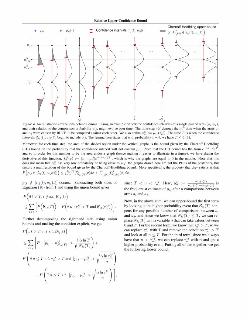
Figure 4. An illustrations of the idea behind Lemma 1 using an example of how the confidence intervals of a single pair of arms (ai, aj),and their relation to the comparison probability pij , might evolve over time. The time-step τ ijm denotes the mth time when the arms aiand aj were chosen by RUCB to be compared against each other. We also define µijm := µij(τ
ijm). The time T is when the confidence
intervals [lij(t), uij(t)] begin to include pij . The lemma then states that with probability 1− δ, we have T ≤ C(δ).
Moreover, for each time-step, the area of the shaded region under the vertical graphs is the bound given by the Chernoff-Hoeffding(CH) bound on the probability that the confidence interval will not contain pij . Note that the CH bound has the form e−(x−µijn )2
and so in order for this number to be the area under a graph (hence making it easier to illustrate in a figure), we have drawn thederivative of this function, f ijn (x) := |x − µijn |e−(x−µijn )2 , which is why the graphs are equal to 0 in the middle. Note that thisdoes not mean that µijn has very low probability of being close to pij : the graphs drawn here are not the PDFs of the posteriors, butsimply a manifestation of the bound given by the Chernoff-Hoeffding bound. More specifically, the property that they satisfy is thatP(pij /∈ [lij(t), uij(t)]
)≤∫ lij(t)−∞ f ijNij(t)(x)dx+
∫∞uij(t)
f ijNij(t)(x)dx.
pij /∈ [lij(t), uij(t)] occurs. Subtracting both sides ofEquation (10) from 1 and using the union bound gives
P(∃ t > T, i, j s.t. Bij(t)
)
≤∑
i<j
[P(Bij(T )
)+ P
(∃n : τ ijn > T and Bij(τ ijn )
)].
Further decomposing the righthand side using unionbounds and making the condition explicit, we get
P(∃ t > T, i, j s.t. Bij(t)
)
≤∑
i>j
[P
(∣∣∣pij − µijNij(T )
∣∣∣ >√
α lnT
Nij(T )
)+
P
∃n ≤ T s.t. τ ijn > T and
∣∣pij − µijn∣∣ >
√α ln τ ijnn
+ P
∃n > T s.t.
∣∣pij − µijn∣∣ >
√α ln τ ijnn
],
since T < n < τ ijn . Here, µijn :=wij(τ
ijn )
wij(τijn )+wji(τ
ijn )
isthe frequentist estimate of pij after n comparisons betweenarms ai and aj .
Now, in the above sum, we can upper-bound the first termby looking at the higher probability event that Bij(T ) hap-pens for any possible number of comparisons between aiand aj , and since we know that Nij(T ) ≤ T , we can re-placeNij(T ) with a variable n that can take values between0 and T . For the second term, we know that τ ijn > T , so wecan replace τ ijn with T and remove the condition τ ijn > Tand look at all n ≤ T . For the third term, since we alwayshave that n < τ ijn , we can replace τ ijn with n and get ahigher probability event. Putting all of this together, we getthe following looser bound:
Relative Upper Confidence Bound
P(∃ t > T, i, j s.t. Bij(t)
)
≤∑
i<j
[P
(∃n ∈ {0, . . . , T} :
∣∣pij − µijn∣∣ >
√α lnT
n
)
+ P
(∃n ∈ {0, . . . , T} :
∣∣pij − µijn∣∣ >
√α lnT
n
)
+ P
(∃n > T s.t.
∣∣pij − µijn∣∣ >
√α lnn
n
)]
≤∑
i<j
[2
T∑
n=0
P
(∣∣pij − µijn
∣∣ >√α lnT
n
)
+
∞∑
n=T+1
P
(∣∣pij − µijn
∣∣ >√α lnn
n
)]. (11)
To bound the expression on line (11), we apply theChernoff-Hoeffding bound, which in its simplest formstates that given i.i.d. random variablesX1, . . . , Xn, whosesupport is contained in [0, 1] and whose expectation satis-fies E[Xk] = p, and defining µn := X1+···+Xn
n , we haveP (|µn − p| > a) ≤ 2e−2na2 . This gives us
P(∃ t > T, i, j s.t. Bij(t)
)
≤∑
i<j
2
T∑
n=1
2e−2�n
α lnT
�n +
∞∑
n=T+1
2e−2�n
α lnn
�n
=K(K − 1)
2
[T∑
n=1
4
T 2α+
∞∑
n=T+1
2
n2α
]
≤ 2K2
T 2α−1+K2
∫ ∞
T
dx
x2α, since
1
x2αis decreasing.
≤ 2K2
T 2α−1+K2
∫ ∞
T
dx
x2α
=2K2
T 2α−1+
K2
(1− 2α)x2α−1
∣∣∣∣∞
T
=(4α− 1)K2
(2α− 1)T 2α−1. (12)
Now, since C(δ) =(
(4α−1)K2
(2α−1)δ
) 12α−1
for each δ > 0, thebound in (12) gives us (9).
8.3. Proof of Theorem 5
Here, we provide the proof of the expected regret boundclaimed in Theorem 5, starting by repeating the statementof the theorem:
Theorem 5. Given the setup of Proposition 2 together withthe notation of Theorem 4, we have the following expectedregret bound for RUCB, where the expectations are takenacross different runs of the algorithm: if we have α > 1, theexpected regret accumulated by RUCB after T iterations isbounded by
E[RT ] ≤[
8 +
(2(4α− 1)K2
2α− 1
) 12α−1 2α− 1
α− 1
]∆max
+ 2D∆max ln 2D +
K∑
j=2
2α (∆j + 4∆max)
∆2j
lnT.
(13)
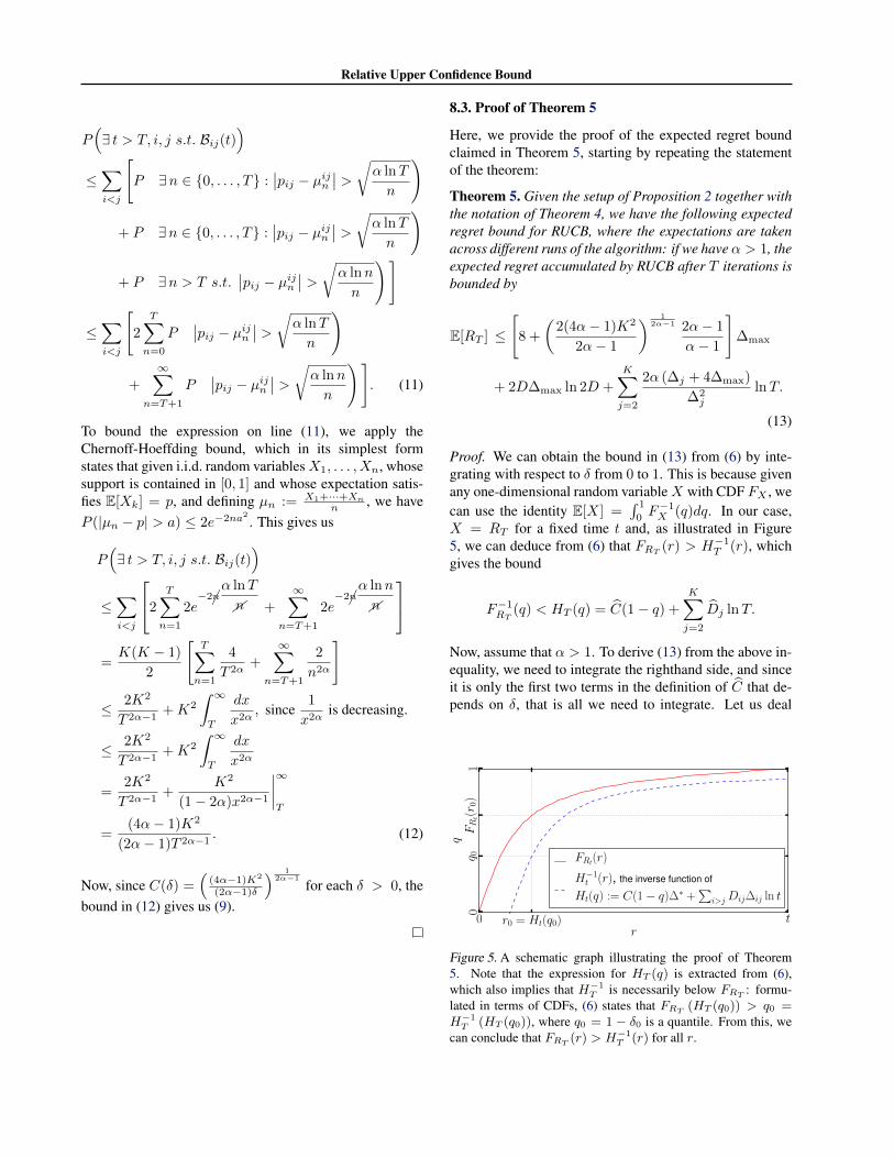
Proof. We can obtain the bound in (13) from (6) by inte-grating with respect to δ from 0 to 1. This is because givenany one-dimensional random variableX with CDF FX , wecan use the identity E[X] =
∫ 1
0F−1X (q)dq. In our case,
X = RT for a fixed time t and, as illustrated in Figure5, we can deduce from (6) that FRT (r) > H−1
T (r), whichgives the bound
F−1RT
(q) < HT (q) = C(1− q) +
K∑
j=2
Dj lnT.
Now, assume that α > 1. To derive (13) from the above in-equality, we need to integrate the righthand side, and sinceit is only the first two terms in the definition of C that de-pends on δ, that is all we need to integrate. Let us deal
0 r0 = Ht(q0) tr
01
q 0FRt(r 0
)q
FRt(r)
H−1t (r), the inverse function of
Ht(q) := C(1− q)∆∗ +∑
i>jDij∆ij ln t
Figure 5. A schematic graph illustrating the proof of Theorem5. Note that the expression for HT (q) is extracted from (6),which also implies that H−1
T is necessarily below FRT : formu-lated in terms of CDFs, (6) states that FRT (HT (q0)) > q0 =H−1T (HT (q0)), where q0 = 1 − δ0 is a quantile. From this, we
can conclude that FRT (r) > H−1T (r) for all r.

Relative Upper Confidence Bound
103 104 105 106
time
0.0
0.2
0.4
0.6
0.8
1.0be
stra
nker
rate
(acc
urac
y)LETOR NP2004 Dataset with 16 rankers
RUCB α = 0.51
Condorcet SAVAGEBTM
103 104 105 106
time
0.0
0.2
0.4
0.6
0.8
1.0
best
rank
erra
te(a
ccur
acy)
LETOR NP2004 Dataset with 32 rankers
103 104 105 106
time
0.0
0.2
0.4
0.6
0.8
1.0
best
rank
erra
te(a
ccur
acy)
LETOR NP2004 Dataset with 64 rankers
Figure 6. Average accuracy for 100 runs of BTM, Condorcet SAVAGE and RUCB with α = 0.51 applied to three K-armed duelingbandit problems with K = 16, 32, 64. Note that the x-axes in these plots use a log scale.
with the first term first, using the substitution 1 − q = δ,dq = −dδ:∫ 1
q=0
4∆max ln2
1− q dq = 4∆max
[ln 2−
∫ 0
δ=1
− ln δ dδ
]
= 4∆max
[ln 2−
∫ 1
δ=0
ln δ dδ
]
= 4∆max(ln 2 + 1) < 8∆max
To deal with the second term in C, recall that it is equal to
2∆maxC(δ2
):= 2∆max
(2(4α−1)K2
(2α−1)δ
) 12α−1
, so to simplifynotation, we define
L := 2∆max
(2(4α− 1)K2
2α− 1
) 12α−1
.
Now, we can carry out the integration as follows, again us-ing the substitution 1− q = δ, dq = −dδ:
∫ 1
q=0
C(1− q)dq =
∫ 0
δ=1
−C(δ)dδ
=
∫ 1
0
2
(2(4α− 1)K2
(2α− 1)δ
) 12α−1
dδ
= L
∫ 1
0
δ−1
2α−1 dδ
= L
[δ1− 1
2α−1
1− 12α−1
]1
0
=
(2(4α− 1)K2
2α− 1
) 12α−1 2α− 1
α− 1.
8.4. Experimental Details
Our experimental setup is built on real IR data, namely theLETOR NP2004 dataset (Liu et al., 2007). This dataset isbased on the TREC Web track named-page finding task,where a query is what the user believes to be a reasonableestimate of the name of the webpage she is seeking. Us-ing this data set, we create a set of 64 rankers, each corre-sponding to a ranking feature provided in the data set, e.g.,PageRank. The ranker evaluation task in this context corre-sponds to determining which single feature constitutes thebest ranker (Hofmann et al., 2013b).
To compare a pair of rankers, we use probabilistic inter-leave (PI) (Hofmann et al., 2011), a recently developedmethod for interleaved comparisons. To model the user’sclick behavior on the resulting interleaved lists, we employa probabilistic user model (Hofmann et al., 2011; Craswellet al., 2008) that uses as input the manual labels (classi-fying documents as relevant or not for given queries) pro-vided with the LETOR NP2004 dataset. Queries are sam-pled randomly and clicks are generated probabilistically byconditioning on these assessments in a way that resemblesthe behavior of an actual user (Guo et al., 2009).
Following (Yue & Joachims, 2011), we first used the aboveapproach to estimate the comparison probabilities pij foreach pair of rankers and then used these probabilities tosimulate comparisons between rankers. More specifically,we estimated the full preference matrix by performing 4000interleaved comparisons on each pair of the 64 featurerankers.
Finally, the plots in Figure 6 show the accuracy of all threealgorithms across 100 runs, computed at the same timesas the exploration horizons used for BTM and SAVAGE inFigure 2. Note that RUCB reaches the 80% mark almosttwice as fast as Condorcet SAVAGE, all without knowingthe horizon T . The contrast is even more stark when com-paring to BTM.