Embed Size (px)
Citation preview

I m I s-2
' r C
f V) ld 0
RELATIVE SIDEBAND AMPLITUDES a 4-
:a- urn , * C 2 3 N
VS. MODULATION a
r- INDEX FOR COMMON FUNCTIONS USING
m o' a FREQUENCY AND PHASE MODULATION
FRANK STOCKLIN
, .4 .* 2 - . . 0
CY + 4 U
0 O W 0 m u
4 c a b m . 4' z* k
-* - a m T.- k- p14hU
.6 - Q S U Z H W Z
.i - V) a n
% 3
5 w o o m m H W t H W C G
p elat4 4 4 A
4 3 0 4 .. - w L 3 z m
i*OH-14 m n = 3
AV) l -3 '4Z r V ) z o InffiUH ornun C I * C ( I I O I xV)==I I M 3 Q E Q k 0 $33 E 8 H a
;
I ' 4 n o w
- 6000ARO SPACE F L H t CENTER CMEIWELT, MARYUIID
https://ntrs.nasa.gov/search.jsp?R=19740002895 2020-03-18T18:28:26+00:00Z
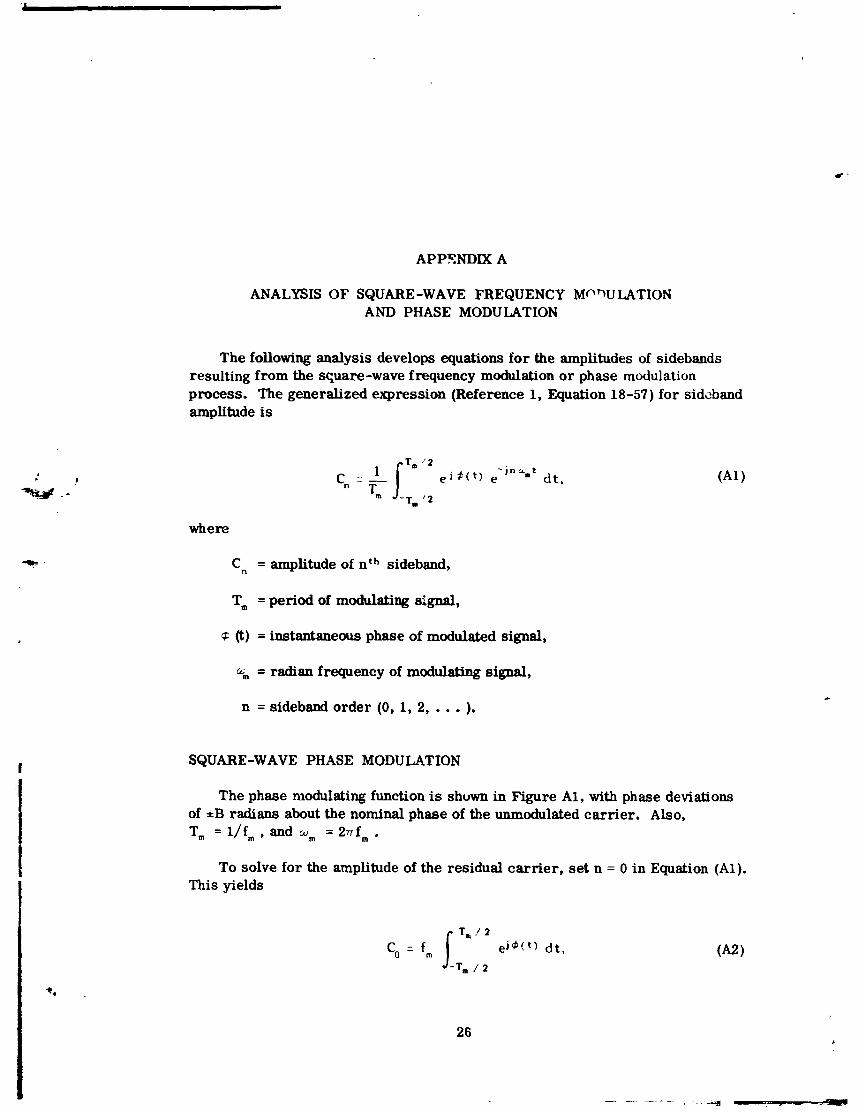
RELATIVE SIDEBAND XMPLJTUDES VS. MODULATION INDEX FOR SOME COMMOPj FUNCTIONS USING
FREQUENCY AND PHASE MODULATION
Frank Stocklin
November 1973
Goddard Space Flight Center Greenbelt, Maryland
PRECEDING PAGE BLANg NOT FILMED
RELATIVE SIDEBAND AMPLITUDES VS. MODULATION INDEX FOR SOME COMMON FUNCTIONS USING
FREQUENCY AND PHASE MODULATION
ABSTRACT
The equations defining the amplitude of sidebands resulting from either frequency modulation or phase modulation by either square-wave, sine-wave, sawtooth or triangular modulating functions are presented. Spectral photographs and computer-generated tables of modulation index vs. relative sideband ampli- tudes are also included.
iii
PRECEDING PAGE BLANK NOT FILMED
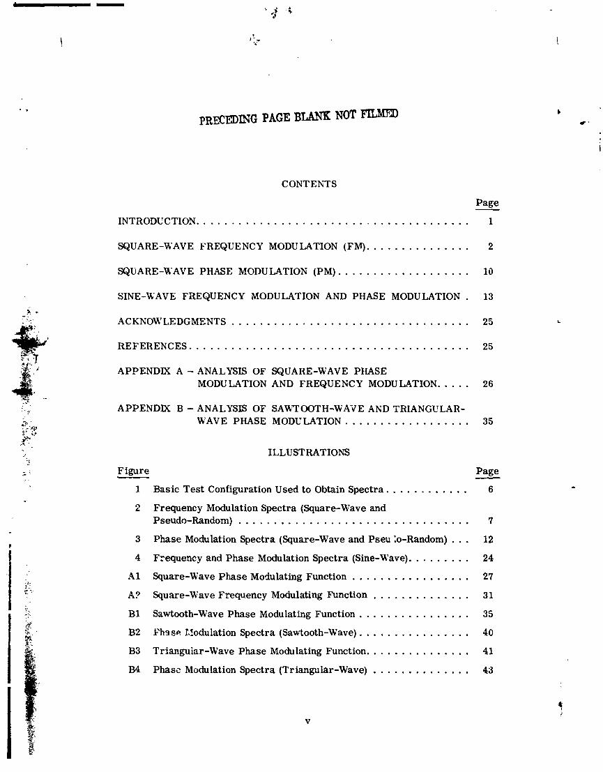
CONTENTS
Page - INTRODUCTION . . . . . . . . . . . . . . . . . . . . . . . . . . . . . . . . . . . . . . . 1
. . . . . . . . . . . . . . SQUARE-WAVE FREQUENCY MODULATION (FM). 2
SQUARE-WAVE PHASE MODULATION (PM). . . . . . . . . . . . . . . . . . . 10
SINE-WAVE FREQUENCY MODULATION AND PHASE MODULATION . 13
ACKNOWLEDGMENTS . . . . . . . . . . . . . . . . . . . . . . . . . . . . . . . . . . 25
REFERENCES . . . . . . . . . . . . . . . . . . . . . . . . . . . . . . . . . . . . . . . . 25
APPENDIX A - ANALYSIS OF SQUARE-WAVE PHASE MODULATION AND FREQUENCY MODULATION. . . . . 26
APPENDIX B - ANALYSIS OF SAWOOTH-WAVE AND TRIANGULAR- WAVE PHASE MODULATION . . . . . . . . . . . . . . . . . . 35
ILLUSTRATIONS
Page - . . . . . . . . . . . 1 Basic Test Configuration Used to Obtain Spectra. 6
2 Frequency Modulation Spectra (Square-Wave and Pseudo-Random) . . . . . . . . . . . . . . . . . . . . . . . . . . . . . . . . . 7
. . . 3 Phase Modulation Spectra (Square-Wave and Pseu 10-Random) 12
. . . . . . . . 4 Frequency and Phase Modulation Spectra (Sine-Wave). 24
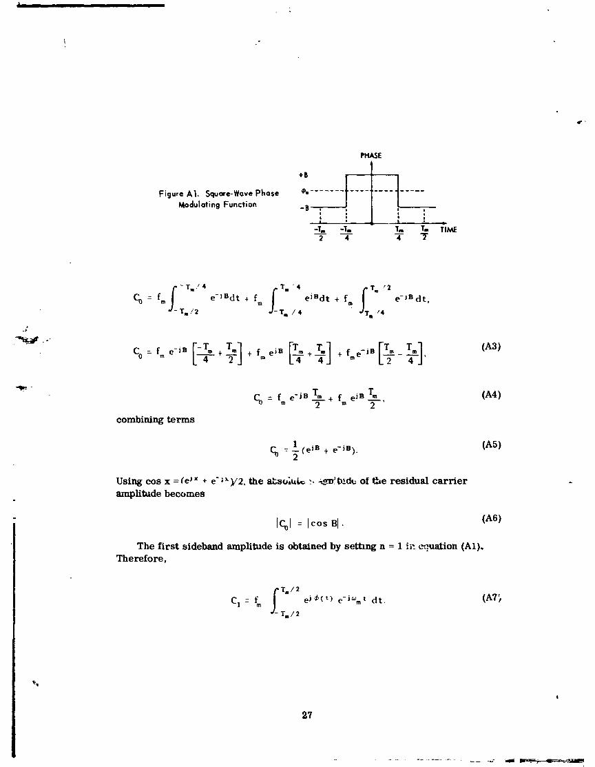
A1 Square-Wave Phase Modulating Function . . . . . . . . . . . . . . . . . 27
. . . . . . . . . . . . . . A? Square-Wave Frequency Modulating Function 31
B1 Sawtooth-Wave Phase Modulating Function . . . . . . . . . . . . . . . . 35
. . . . . . . . . . . . . . . . B2 Phn se f.!odulation Spectra (Sawtooth-Wave) 40
. . . . . . . . . . . . . . B3 Trianguiar-Wave Phase Modulating Function. 41
. . . . . . . . . . . . . . B4 Phase Modulation Spectra (Triangular-Wave) 49
RELATIVE SIDEBAND AMPUTUDES VS. MODULATION INDEX FOR SOME COM.LION FUNCTIONS USING
FREQUENCY AND I~HASE MODULATION
INTRODUCTION
An important consideration in the. design and testing of a communications system is the relative amplitude of sirleband components resulting from modu- lation of a radio frequency (RF) carx5er. This spectral information is useful in compatibility testing to determine modulation parameters and can also be used to precisely select optimum receiver bandwidths. This document is intended to be used as a handbook for engineers involved in such activities. The majority of the information is presented in tabular form (i.e. modulation index vs. relative sideband amplitudes). Spectrum photographs a re included for illustrative purposes. Theoretical background material is given for completeness and convenience.
Appendix A contains the square-wave F M and P M analysis and develops the equatioas for the sideband amplitudes.
Appendix B extends the P M analysis for the sawtooth and triangular modu- lating function. This illustrates the generality of the analysis technique.
The general expression (derived in Appendix A) for the amplitude of the nth sideband resulting from square-wave frequency modulation of a unity-amplitude RF carrier is
Taking the limit as ,b - n
R F carrier deviation bf ) where ,B modulittion index in radians = modulating frequency (fm) '
n = sideband order (0, 1, 2, . . . ), J C / = absolute value of nth order sideband.
The expression for the residual carrier amplitude is obtained by setting n = 0 in Equation (1):
Note that the right-hand side of Equation (3) has the form of sin x/x, which has a limit value of 1 asx - 0; for the no-modulation case, the carrier ampli- tude is equal to 1.
The expression for the first sideband amplitude term (n = 1) is
A convenient ratio for measurement purposes is the ratio the residual carrier amplitude to the firs' ie r sideband amplitude. This ratio is given by
This result can bc used to determine the relative difference between the residual carrier level and the first sideband level on a spectrum analyzer. Expressions for the higher-order sidebands are given in Appendix A. Table 1 contains the solution of Equation (1) for the first five sidebands for modulation indices up to 10; all sideband amplitudes are nor~,~:dized to unity as follows:
Relative sideband amplitude = 20 log ,, (1/ c,I ) = -20 log,, / C , i . Table 2 illustrates the use of Table 1. Unrnodulated carrier power level:
1 watt (30 dbm) ; Fhl mod index = 1.
The following salient properties df square-wave frequency modulation should be noted:
(a) The residual carrier is zero for all even-integer modulation indices;
@) When 3 i s an odd integer, the odd-ordered sidebands equal zero (except the 3 = n sideband);
(c) When 3 is an even integer, the even-order sidebands equal zero (except the 9 = n sided and);
(d) When ,b = n, one-half the spectral energy resides in the i j: = n sideband; the remaining spectral energy is contained in the residual carrier and other sidebands ;
(e) Except for the special cases noted previou=ly, all sidebands are present in the FM spectrum although only odd harmonics exist in the modulating signal.
Figure 1 illustrates the basic test setup used to obtain spectrum photographs, These photographs are shown in Figure 2. The modulation indices were chosen to demonstrate the spectrum characteristics discussed previously. A decibel scale (phot~g~aph (e)) is provided for measuring amplitudes from the p i c t u ~ s . This scale is valid for all RF spectrum photographs in Figures 2, 3, 4, B1 and B4. For each modulation index, the corresponding spectrum resulting from the equivalcct pseudo-random (PR) modulating signal is shown.* This is done both because the PR spectrum is a good approximation to the actual spacecraft data spectrum, and also to illustrate the problem in the setting of modulation index for complex signals.
* Equivalent PR sign01 is defined os follows: Assilme t i e square wove to be gerleroted by u s i ~ g
on alternating 1,0 NRZ-L pottern. The PR code i s then clocked at the same square-wove rate, but with its own unique 1,0 pattern.
3
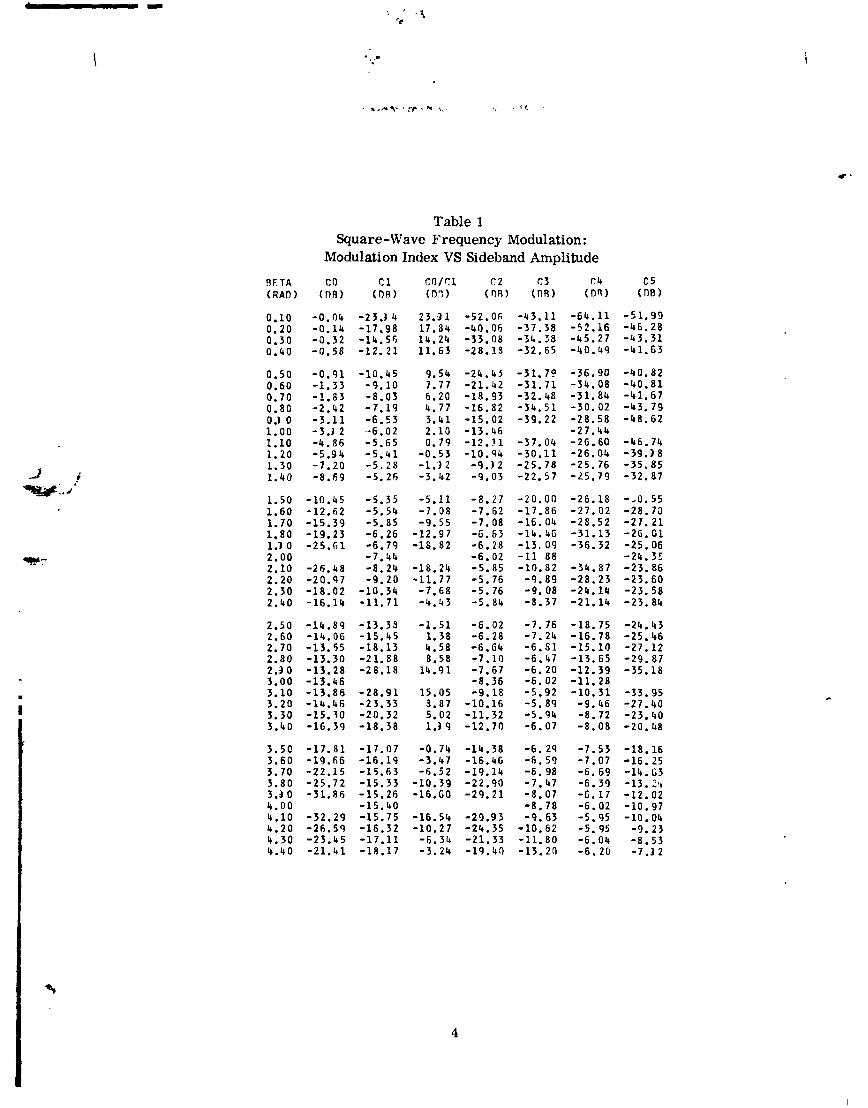
Table 1 Square-Wave Frequency Modulation:
Modulation Index VS Sideband Amplitude
c0 c 1 co/c1 c 2 c3 c 4 ( D R ) (DR) (nn) (OR) ( n ~ ) (DR)
-0.04 -23.3 4 23.31 -52.06 -43.11 -64.11 -0.14 -17.98 17.34 -40.06 -37.38 -52.16 -0.32 -14.56 14.24 -33.08 -34.38 -45.27 -0.58 -12.21 11.63 -28.13 -32.65 -40.49
-0.91 -10.45 9.54 -24.43 -31.79-36.90 -1.33 -9.10 7.77 -21.42 -31.71 -34.08 -1.83 -8.03 6.20 -18.93 -32.48 -31.84 -2.42 -7.19 4.77 -16.82 -34.51 -30.02 -3.11 -6.53 3.41 -15.02 -39.22 -28.58 -3.1 2 46.02 2.10 -13.46 -27.44 -4.86 -5.65 0.79 -12.11 -37.04 -26.60 -5.94 -5.41 -0.53 -10.94 -30.11 -26.04 -7.20 -5.28 -1.32 -9.12 -25.78 -25.76 -8.69 -5.26 -3.42 -9.03 -22.57 -25.79
-10.45 -5.35 -5.11 -8.27 -20.00 -26.18 -12.62 -5.54 -7.08 -7.62 -17.86 -27.02 -15.39 -5.85 -9.55 -7.08 -16.04 -28.52 -19.23 -6.26 -12.97 -6.63 -14.46 -31.13 -25.61 -6.79 -18.82 -6.28 -13. 09 -36.32
-7.44 -6.02 -11 88 -26.48 -8.24 -18.24 -5.85 -10.82 -34.87 -20.97 -9.20 -11.77 -5.76 -9.89 -28.23 -18.02 -10.34 -7.68 -5.76 -9.08 -24.14 -16.14 -11.71 -4.43 -5.84 -8.37 -21.14
BETA ( RAD 1
0.10 0.20 0.30 0.40
0.50 0.60 0.70 0.80 0.) 0 1.00 1.10 1.20 1.30 1.40
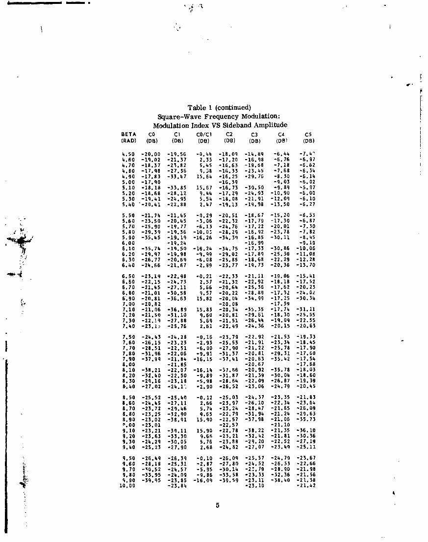
Table 1 (continued) Square-W ave Frequency Modulation :
Modulation Index VS Sideband Amplitude BETA CO C 1 CO/Cl c2 C 3 C4 C5 (RAD) (DB) (DB) (DB) (DB) (DB) (DB) (DB)
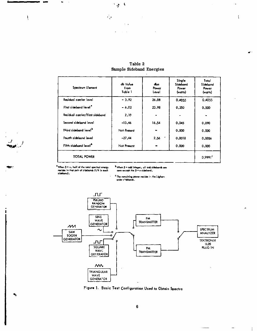
Table 2 Sample Sideband Energies
' ~hmn B = n, half of the totol ~p.ctrul e w b ~ n p =odd integer, oll odd sibbond m raidrr in t M pair of s i & M (1/4 in ~h 1.m except the B = n ribbmd. ridoband).
T h . m i n i * ) power midm in the :,igh.r- abr *:.&on&.
RANDOM GENERATOR
Spectrum Element
Residual carrier Iwel
Fint sideband lwel'
Residual carrier/Fint sideband
Second sidebad level
Third sideband levelb
Fourth ridebond lwel
Fifth sidebnd levelb
TRANSMITTER i
db Value From
Table 1
- 3.92 - 6.02 2.10
-1 3.46
Not Resent
-27.44
Not Present
pc-1 1 WAVE
Total Sidebnd
Power (watts)
0 .a055
0.500
- 0.090
0 .OOO
0.0036
0 .000
TOTAL POMR
dbm Power Lwel
26.08
23.98
- 1 6.54 - 2.56 '
Q
SPECTRUM ANALYZER
TOOTH TEKTRONIX - 1 L20
SQUARE PM PLUG IN WAVC TRANSMITTER
,GEP!ERATOW
0.9991'
Siqle Sidebond
Pcwer (watts)
0 A055
0.250
- 0.045
0 .OW
0.0018
0 .OOO
TRIANGULAR
GENERATOR
Figure 1. Basic Test Configuration Used to Obtain Spectra

Figure 2, Frequency Modulation Spectto (Square-Wove ond P seudo- Pondom)
7
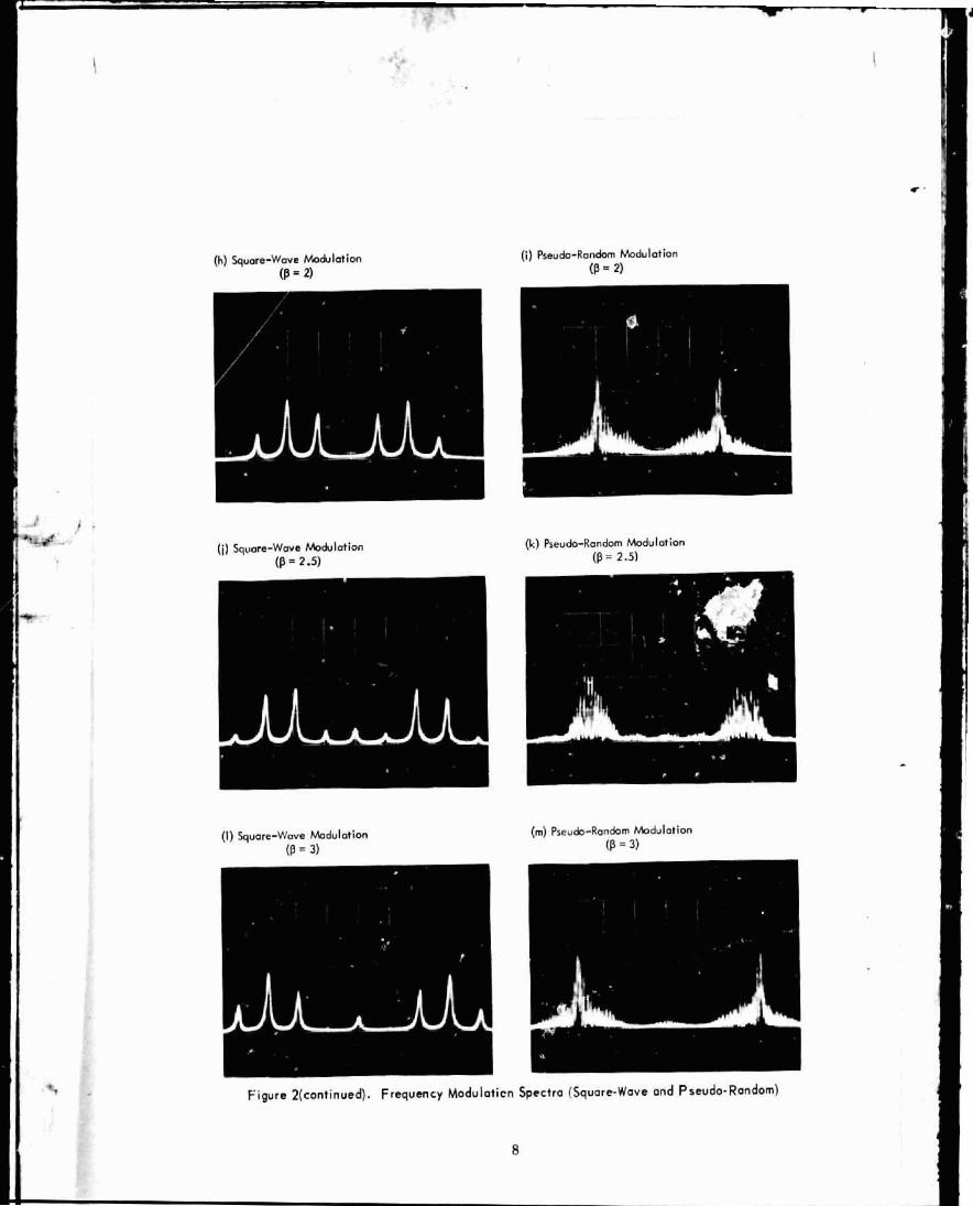
(h) 5q~0rn-Wme Wobldlon (i) Pseudo-Ron& Modulation IR a 91 (P = 2)
(1) Squore-Wave bduld ion (m) Re"&-Ron&m F-rbdtllotion rn = 71 (P = 3)
Figure 2(continued). Frequency Modulotien Spectra Isquare-Wove ond Pseudo-~ondom)
8
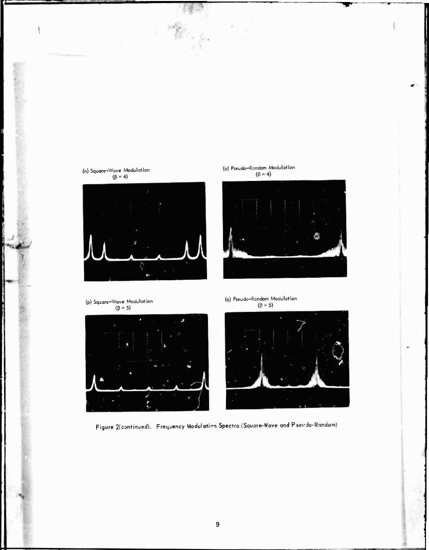
(n) 5qume-Wme Modulation
Iq) Re"&-R~ndom Modulmtion
Figure 2(continucd). Fres~sncy Modulntien Spectra { b u a r r Wave and Pswdo-Random)
9
SQUXRE-WAVE PHASE MODULATION (PM)
Appendix A contains the derivation of the eqcations for ihe sideban< ampli- tudes for this modulation case. Table 3 contains the solution of thene equations for modulation ind!ces up to 3 radians; this is the normal range ~f interest because most PSI schemes require a low index to ensure aclequate residual carr ier power for phase lock demodulation and tracki-4. The significant PhI spectral properties are:
(a) the P M spectrum is not the came as the FM spectrum, even for thc same modulation index;
(b) no even-order sidebands a re present in the resultant spectrum;
(c) the residual carr ier goes to zero at a modulation index of .r ,'2 (or any multiple of n / 2 ) radians.
In general, the square-wave PM process can be viewed simply as amplitude moduIation of the RF carr ier by the modulating spectrum. If one considers the baseband spectrum as double-sided (i.e., containing both positive and negative image frequency components), then this spectrum is simply translated up in frequency ~ymrr~etrically placed about the RF carrier. Only those frequency components existing in the modulating spectrum wil l be present in the P M spectrum. This point can be illustrated by writing the expression for the P M wave as
f ( t ) = A c o s ( z C t + ,L?C(t)), where
A = amplitude of signal
= radiancarrierfrequency
C(t) = modulating function
2 = peak phase deviation of carr ier frequency in radians.
The modulating signal is restricted to values of *1. This representation is valid for the PR signal o r any binary function. Expanding Equation (6) yields
f ( t ) = A c o s u c t cos,,3C(t) - A s i n cict sin,.?C(t). (7
Allowing C(t) = *l, then
c o s f i C ( t ) - c o s ,?
s i n P C ( t ) - C ( t ) s i n !?.
and so
f ( t ) = A cos dc t cos -3 -AC( t ) sin 2 s i n kct.
The first term in Equation (9) is simply the in-phase carrier term.
The second term has the form of amplitude modulation of the quadrature carrier component by C(t) sin 3 . As previously stated, this means that the baseband spectrum of the digital signal is translated in frequency symmetrically about the RF carrier frequency. The spectrum pictures are shown in Figure 3.
For modulating signals other than the square-wave binary type, a unique analysis must be performed. This is d o ~ e in Appendix B for a sawtooth and triangular function. Theoretically, the analysis can be done for any signal that is expressable by an equation; however, the mathematics becomes rather complex for other than simple functions.
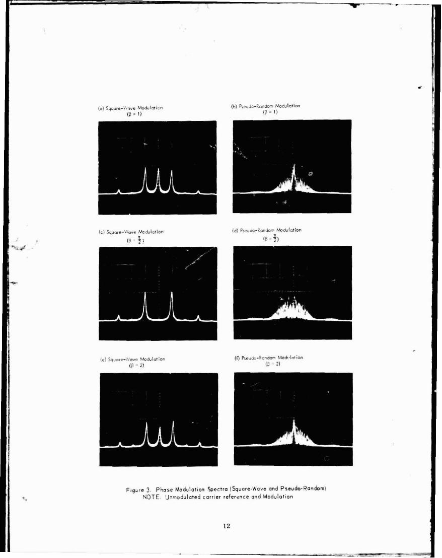
F~gure 3. Phase Modulation k e c t NQTE. trnmodulated carrier
*ra [Square-Wove ond Pseuda-Rondoml reference and Modulation
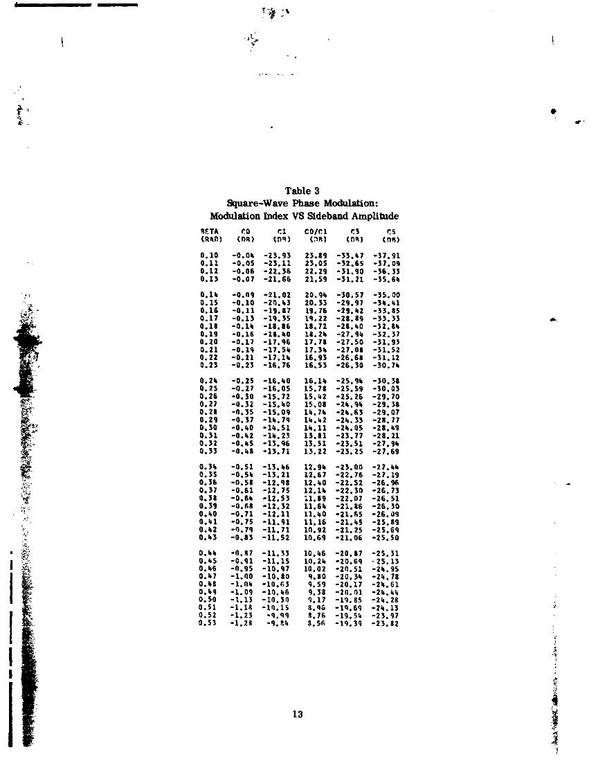
Table 3 Square-W ave Phase Modulation:
Modulation Index VS Sideband Amplitude RETA tO Cl COlCl t 3 C5 (R4D) ( n R ) ( D R ) (nR) (OR) ( D R )
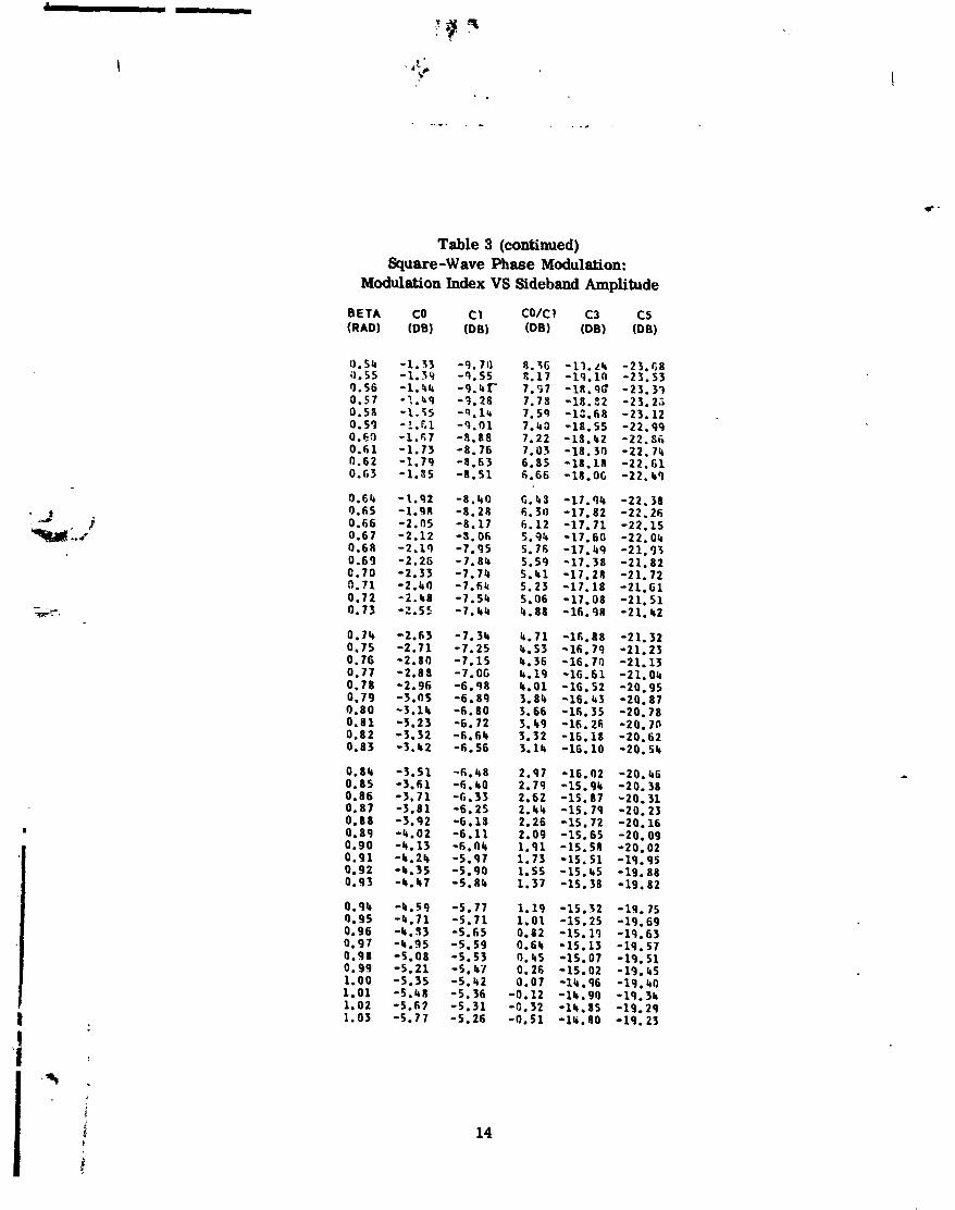
Table 3 (continued) Square-W ave Phase Modulation:
Modulation Index VS Sideband Amplitude
BETA CO C1 Co/C l C3 CS (RADI (DB) (oe) ( 0 s ) (DB) (DB)
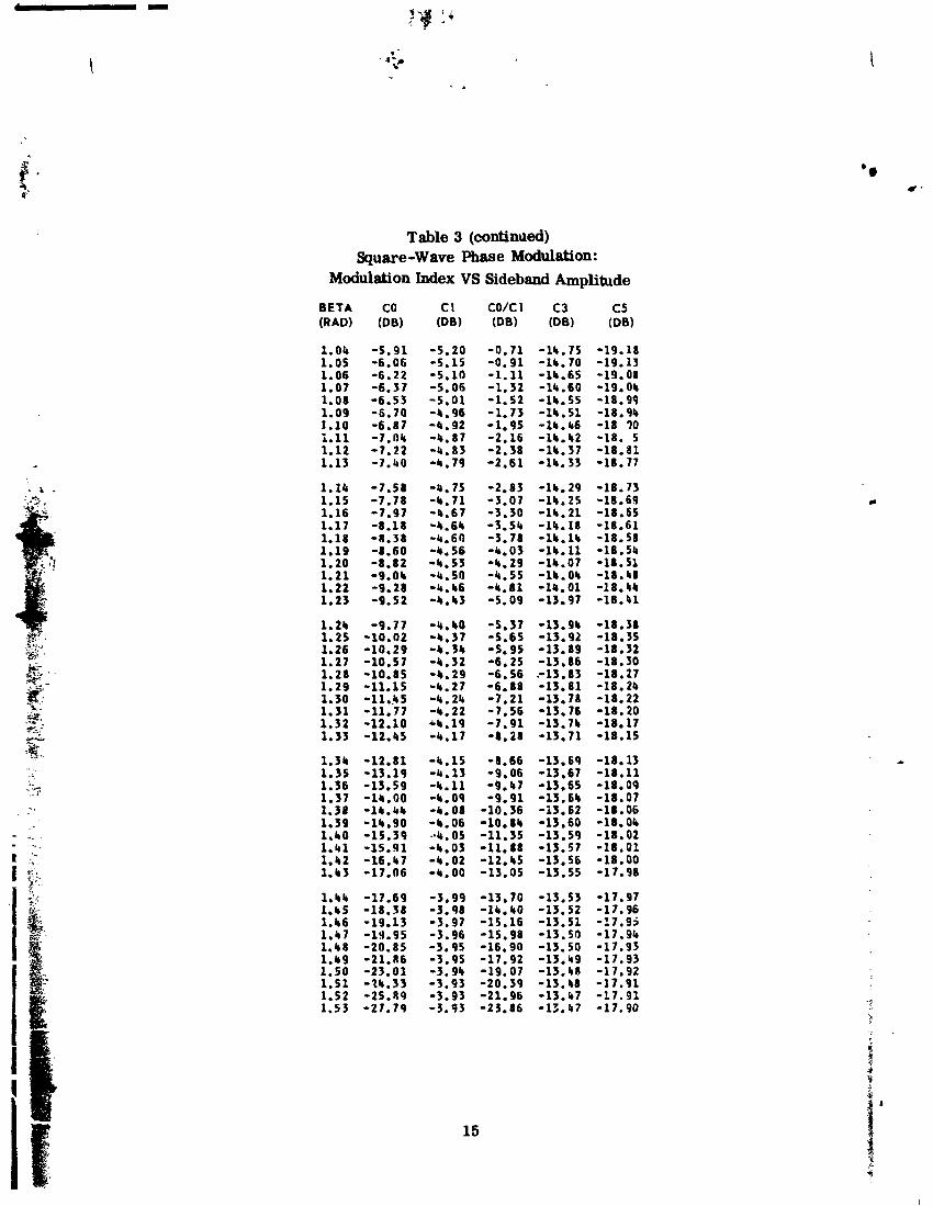
Table 3 (continued) Square-W ave Phase Modulation:
Modulation Index VS Sideband Amplitude
BETA CO C1 CO/C1 C3 C5 (RAD) (DB) (OBI (DB) (DB) (DB)

Table 3 (continued) Square-W ave Phase Modulation:
Modulation Index VS Sideband Amplitude BETA CO C1 CO/Cl c 3 CS ( R A W (DB) (OBI (06 ) (DB) (DB) 1.54 -30.23 -3.92 -26.31 -13.16 -17.90 1.55 -33.64 -3.92 -29.72 -13.16 -17.90 1.56 -39.33 -3.92 -35.42 -13.46 -17.90 1.57 -3.92 -58.06 -13.16 -17.90 1.58 -50.72 -3.92 -36.80 -13.16 -17.90 1.59 -34.33 -3.92 -30.11 -13.46 -17.90 1.60 -30.69 -3.92 - -26.77 -13. 46 -17.90 1 .61 -28.14 -3.92 -24.21 -13.47 -17.90 1.62 -26.16 -3.93 -22.21 -13.47 -17.91 '1.63 -24.56 -3.93 -20.62 -13.18 -17.91
1.64 -23.20 -3.94 -19.27 -13.48 -17.92 1.65 -22.03 -3.95 -18.09 -13.49 -17.92 1.66 -21.00 -3.95 -17.05 -13.50 -17.93 1.67 -20.08 -3.96 -16.12 -13.50 -17.94 1.68 -19.25 -3.97 -15.28 -13.51 -17.95 1.69 -18.19 -3.98 -14.51 -13.52 -17.96 1.70 -17.80 -3.99 -13.81 -13.53 -17.97 1.71 -11.16 -4.00 -13.15 -13.51 -17.98 1.72 -16.56 -1.02 -12.55 -13.56 -17.99 1.73 -16.00 -4.03 -11.97 -13.57 -18.01
1.74 1 5 . 4 7 -4 .01 -11.43 -13.59 -18.02 1.75 -10.98 -4.06 -10.92 -13.60 -18.04 1.76 -14.51 -4.07 -10.44 -13.62 -18.05 1.77 - 1 4 0 7 -4 .09 -9.98 -13.63 -18.07 1.78 -13.65 -4.11 -9.54 -13.65 -18.09 1.79 -13.25 -4.13 -9.12 -13.67 -18.11 1.80 -12.87 -4.15 -8.72 -13.69 -18.13 1 .81 -12.51 -4.17 -8.34 -13.71 -18.15 1.82 -12.16 -4.19 -7.97 -13.73 -18.17 1.83 -11.82 -4.21 -7.61 -13.76 -18.19
l . 8k -11.50 -4.24 -7.27 -13.78 -18.22 1.85 -11.19 -4.26 -6.93 -13.80 -18.21 1.86 -10.90 -4.29 -6.61 -13.83 -18.27 1.87 -10.61 -b.31 -6.30 -13.86 -18.29 1.88 -10.33 -1.34 -5.99 -13.88 -18.32 1.89 -10.07 -4.37 -5.70 -13.91 -18.35 1.90 -9 .81 -4.40 -5 .41 -13.94 -18.38 1 .91 -9.56 -4.43 -5.13 -13.97 -18 .51 1.92 -9.32 -4.46 -4.86 -14.00 -18.44 1.93 -9.08 -4.49 -4.59 -14.03 -18.17
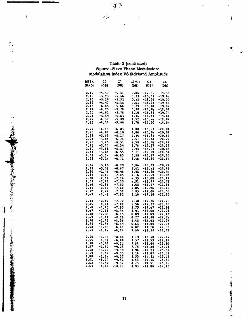
Table 3 (continued) Square -Wave Phase Modulation:
Modulation Index VS Sideband Amplitude
BETA CO C1 CO/Cl C3 CS (RAD) (DB) (DB) (DB) (DB) (DB)
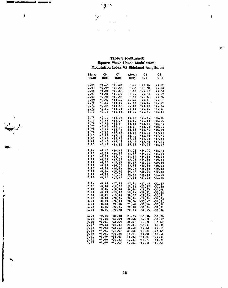
Table 3 (continued) Square-Wave Phase Modulation:
Modulation Index VS Sideband Amplitude
BETA CO C1 CO/Cl C3 C5 (RAD) (DB) (DB) (DB) (DB) (DB)

Most communication theory texts contain the derivation d sideband amplitude for sinusoidal modulation. It is repeated here for convenience, and also to illustrate that in this unique case, F M and P M are essentially the same.
For the F M case, the time function can be represented as
f ( t ) = ~ e ' 't,
where
A = carrier amplitude e 1,
Here,
u t = instantaneous angular frequency,
4, = instantaneous phase of rotating vector.
Now, letting the instantaneous angular frequency be modulated by a sinusoid, we have
w = Oc + Awcos Ult, t
where
w, = angular carrier frequency,
a, = angular frequency of modulating signal,
AU = peak angular frequency excursion from a, due to modulation.
Applying this result to Equation (11) yields
t
4, = I (we + Autos wit) d t .
Integrating Equation (13) yields
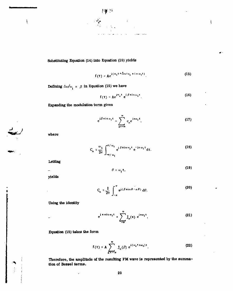
Substitutiqg Equation (14) into Equation (10) yields
Defining Ao/ol . P in Equation (15) we have
jW t j p s i n w , t f (t) = Ae e
Expanding the modulation term gives
where
- yields
j/3 s i n ol t jnwl t e 5
j B s i n ~ , t - j n w l t Cn =- e e d t .
Using the identity
Equation (15) takes the form
Therefore, the amplitude of the resulting FM wave is represented by the summa- tion of Bessel terms.
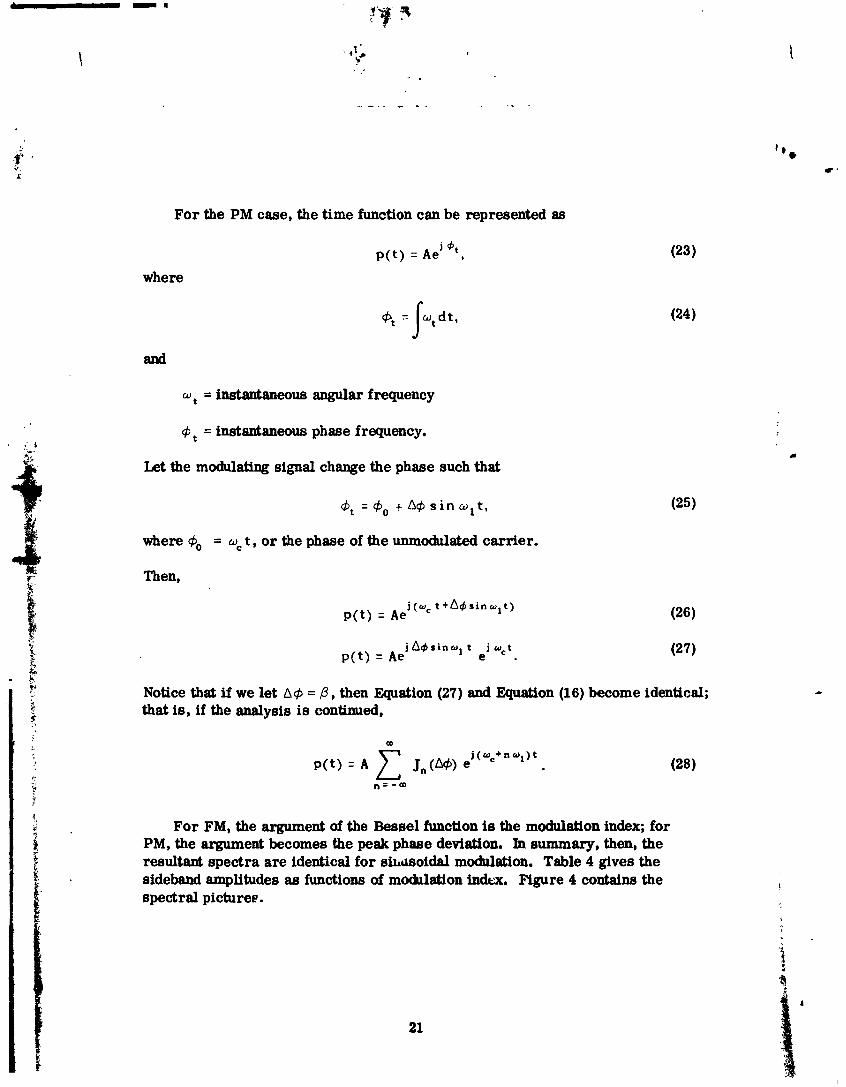
For the PM case, the time function can be represented as
where
and
w , = instantaneous angular frequency
4, = instantaneous phase frequency.
Let the modulating signal change the phase such that
d, = #o + A$ sin wit,
where $,., = wc t , or the phase of the unmodulated carrier.
Then,
Notice that if we let A 4 = P , then Equation (27) and Equation (16) become identical; that is, if the anrilysis is continued,
For FM, the argument of the Beseel function is the modulation index; for PM, the argument becomes the peak phase deviation. In summary, then, the resultant spectra are identical for s imoidal modulation. Table 4 gives the sideband amplitudes as functions of mothlation index. Mgure 4 contains the spectral picturee.
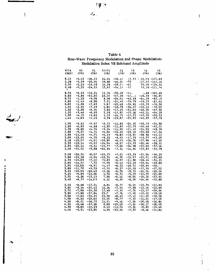
Table 4 Sine-Wave Frequency Modulation and Phase Modulation:
Modulaticn Index VS Sideband Amplitude
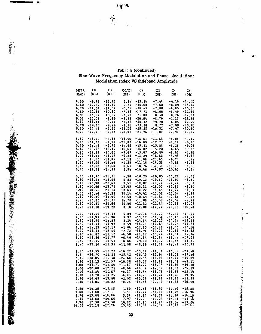
T ~ b l ? 4 (continued) Sine-Wave Frequency Modulation and Phase ,Modulation:
Mo6.ulation Index VS Sideband Amplitude
BETA (RAD)
4.50 4. 6 0 0.70 4.80 4.90 5.00 5.10 5.20 5.30 5.40
5.50 5.60 5.70 5.80 5.30 6.00 6.10 6.20 6.30 6.40
6.50 6.60 6.70 6.80 6.9 0 7.00 7.10 7.20 7.30 7.40
7.50 7.60 7.70 7 .80 7.90 8.00 8.10 8.20 8.30 8.40
8. 5 0 8.6. 8.7 d 8.80 8.90 9.00 9.10 9.20 9.30 9. 40
9.50 9.60 9.70 9.80 9.90
1O.SO

(e) Phma Wld*m r a = l n
(d) Phcec fulwulot* (b=l -J)
ll Figure 4- Frmmcy a d Phase Modulation Spectra (Sine Wave)
The author wishes to thank Mr. Charles Scaffidi and Mr. John B. Martin for providing encouragement, reviewing this document and making many signficant suggestions; he is also grateful to Mr. Earl Turner for providing assistance in the mathematical analyses.
REFERENCES
1. C. L. Cuccia. Harmonics, Sidebands and Transients in Communication -eering. New York: McGraw-Hill, 1952.
2. P. F. Panter. Modulation, Noise, and Spectral Analysis. New York: McGraw- Hill, 1965.
3. S. Golorub, ed., Digital Communications with Space Applications. Contributions by I,. D. Baumert, M. F. Easterling, J. J. Steffler, and A. Viterbi. Englewood Cliffs: Prentice-Hall, Inc., 1964.
4. J. H. Painter and G. Hondros. "Unified S-Band Telecommunication Techniques for Apollo - Volume II.", NASA Technical P: D-3397, Manned Spacecraft Center, April, 1966.
5. R. Pickett. "Signal Generator Calibration." Prepared under Contract No. F04697-67-C-0001. Space and Missile Test Center, Federal Electric Corporation, Los Angeles, California, 1970.
ANALYSIS OF SQUARE-WAVE FREQUENCY MC"XJLATI0N AND PHASE MODULATION
The following analysis develops equations for the amplitudes of sidebands resulting from the quare-wave frequency modulation or phase modulation process. The generalized expression (Reference 1, Equation 18-57) for sideband amplitude is
where
Cn = amplitude of nth sideband,
Tm = period of modulating signal,
3: (t) = instantaneous phase of modulated signal,
= radian frequency of modulating signal,
n = sideband order (0, 1, 2, . . . ).
SQUARE-WAVE PHASE MODULATION
The phase nlodulating function is shown in Figure Al, with phase deviations of *B radians about the nominal phase of the modula ted carrier. Also, T, = l / f , , and urn = 2nfm .
To solve for the amplitude of the residual carrier, set n = 0 in Equation (Al). This yields
PHASE t
Figure A l . Square-Wove Phase Modulating Function -B
combining terms
Using cos x =(eJx + e-jA)/2, the a;;so;kCt 1. i?:h?dt: of the residual carrier amplitude becomes
The first sideband amplitude is obtained by sethng n = 1 11: e:;uation (Al). Therefore,
- .. - - ~ .--- - - I-. 1- Y y . ~
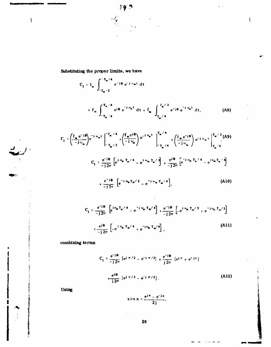
Substituting the proper limits, we have
t f,,, IT'" , j ~ .-J d t t fi. e - j ~ e-J st d t . (AS) -rm '4
jaIrrn/4 t- t e
(A l l )
combining terms
g j B [,J n / 2 - q j n / 2 ] + e
- i B c, = - - [ e ~ " + e-iff] -j2n j 277
.i B +- [ e ~ f f 1 2 - e-j - 1 2 1
i2n
e ~ x - e - j x s i n x =
2 j I
Using

Equation (A12) becomes
e - j B . n e - j B eJB . n C1 = -- s l n - + - s i n n + - s l n - .
n 2 77 7r 2
Taking the absolute magnitude of Equation (A13) yields
Therefore, the ratio of residual carrier level to first sideband amplitude becomes
The second-order sideband ia
e i + ( t ) e -2 i o,t C2 = f, dt .
Substituting the limits yields
. L. * b*, . ,
combiring terms
Therefore, C, = 0. All higher-order even terms in multiples of n and 2 in the above expression would cause all even terms to be zero. Solving for the third sideband amplitude gives
,-jB 3 e - ~ B ej B C = - s i n - n + s i n 3n +-
2 r in a,
-377 3n 3n
2 j C3 = - s i n B . 377
Solving for the fifth- and seventh-order sidcband would yield the expressions:

In general, then,
SQUARE-WAVE FREQUENCY MODULATION
The f requency-modulating function is shown in Figure A2 with frequency deviations of x ~wradlsec about the normal frequency of the unmodulated carrier.
FREQUENCY
w0 + AO
Figure A2. Square-Wove Frequency
Moduloting Function
The instantaneous frequency i s given by
The instantaneous phase is given by

The phase variations about the nominal carrier phase are given by
" = Aot; - < t < - (- 2: 2%
Subetituting these values into Equation (Al), the following general eqression results :
where
UtWJ
dB = w,dt,
changing the limits and setting n = 0 , the carrier term becomes
2 I C ~ I = 1% sin P - . 2 l
Setting n = 1, the first sideband term becomes

Substituting the limits and simplifying, the final expression becomes
If the process is continued for higher-order values of n, the following general expression is obtained:
i.' . :.*,e ,
APPENDIX B
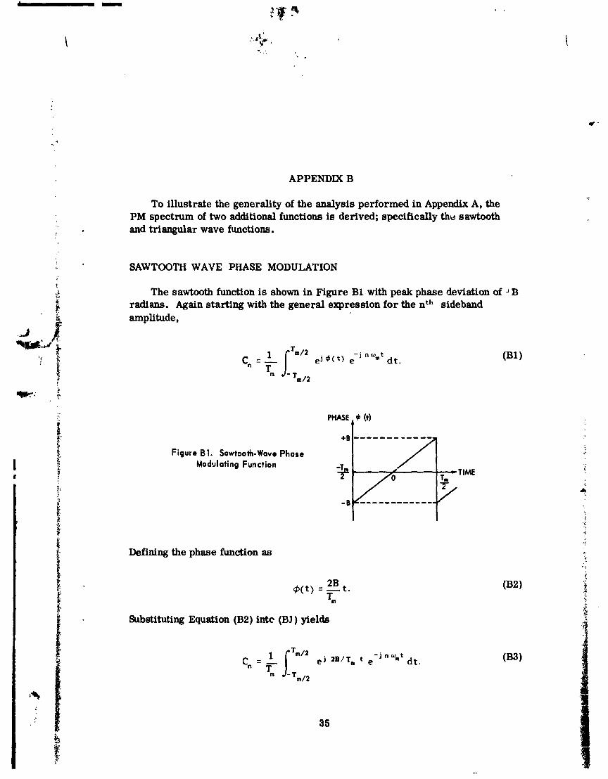
To illustrate the generality of the analysis performed in Appendix A, the PM spectrum of two additional functions is derived; specifically the sawtooth and triangular wave functions.
SAWTOOTH WAVE PHASE MODULATION
The sawtooth function is shown in Figure B1 with peak phase deviation of -I B radians. Again starting with the general expression for the nth sideband amplitude,
1 1"" t ) e - j no,t c,, = - d t . Tm
"m/2
Figure 01. Sawtooth-Wave Phase Moddating Function
Defining the phase function as
Substituting Equation (B2) intc (B1 ) yields
- j n w m t Cn = ,J 28/T, t , d t .
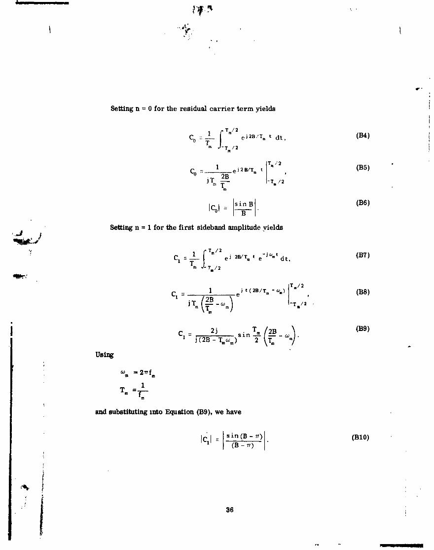
Setting n = 0 for the residual carrier term yields
sin B
Setting n = 1 for the first sideband amplitude .yields
and substituting into Equation (B9), we have
sin (B - n) Ic,I =
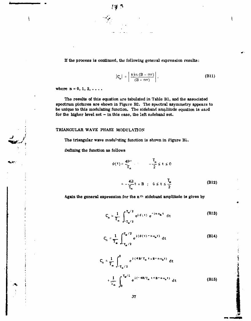
If the process is continued, the following general expression results:
where n = 0,1, 2, . . . . The results of this equation are tabulated in Table B1, and the associated
spectrum pictures are ahown in Figure B2. The spectral asymmetry appears to be unique to this modulating function. The sideband amplitude equation is uszd for the higher level set - in this case, the !eft srdeband set.
TRLANGULAR WAVE PHASE MODUL4TXON
The triangular wave modul ding function is sbovn in Figure BS.
Defining the function as follouls
Again fhe general expression for the nth aideband amplitude is given by

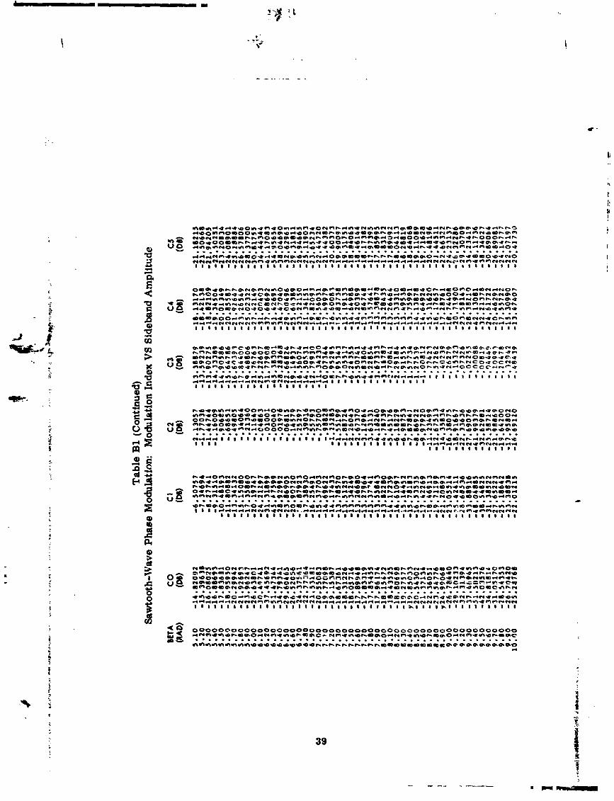
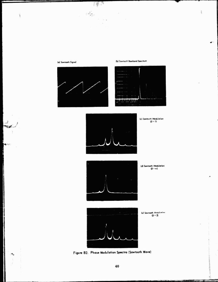
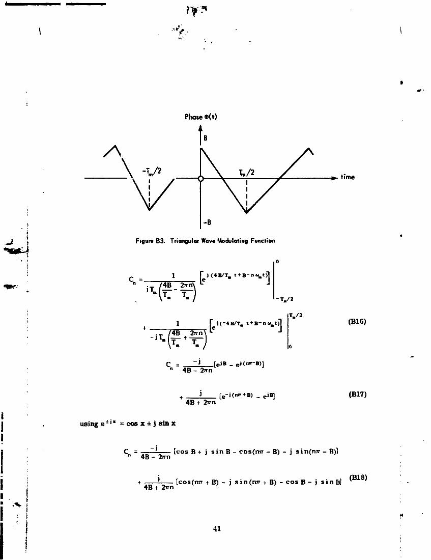
Fig- 83. Triangular Wave rrbblating Function
usingefix =cos x i j sinx

[(s i n B - s in(nn - B)) t j (cos(nn - B) - e c . B); Cn = 4B - m n
+ 1 - [(s in(nn + B) + s i n B) + j (cos(nw + B) - c o s 8); (B19) 4B t 2nn
1 1 s i n x f s i n y = 2 s i n - (x f y) c o s - ( x r y) 2 2
1 1 c o s x + c o s y = 2 c o s -(x + y) c o s - (x -Y) 2 2
1 - 1 c o s x - c o s y = - 2 s i n - (x + y) s i n - ( x - y)
2 2
1 1 1 C, = - 28) cos-(nn)+ j s i n - ( m ) s i n - (nn - 2B)l
nw - 2B 2 2 2
1 1 t n r ' + 2B [ : s i n - (nn + 2B) cas j n r ) 2 - j s i n - 2 (n. + 2B) s i n 2 (m)] (l320),
The final expression then becomes
Ic,l = c o s - nlr m - 2B nn + 2B 2
s i n (!j! -4 - s i n (7 t - nn s i n -
nw + 2B 2
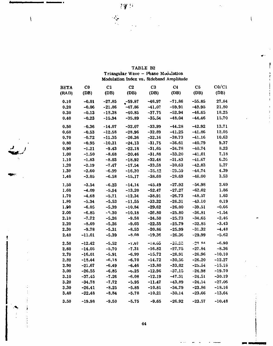
The reaulta of this equation are tabulated in Table E2 and the corresponding spectrum pictures are shown in Figure B4.
j J
1
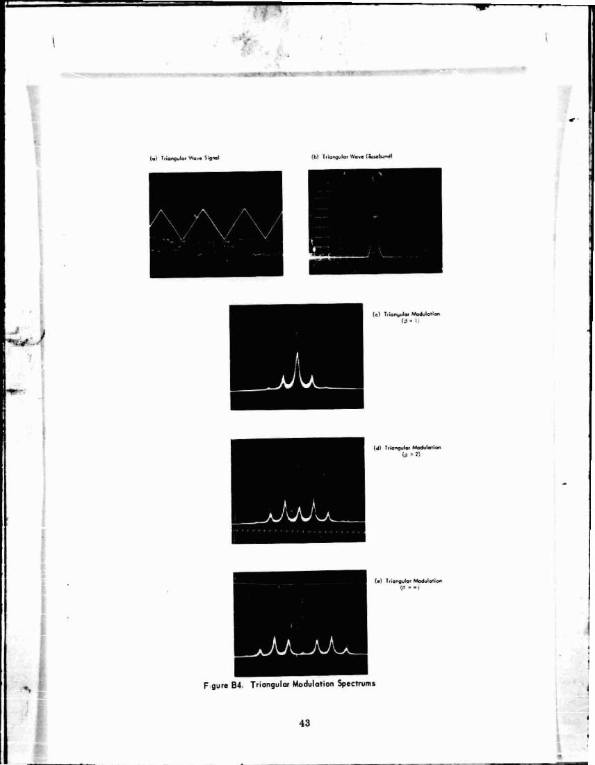
1 % F gure 64. Triangulm Modulation Spectrums
BETA (RAW
0.10 0.20 0.30 0.40
0.50 0.60 0.70 0.80 0.90 1.00 1.10 1.20 1.30 1.40
1.50 1.60 1.70 1.80 1.90 2 .oo 2.10 2.20 2.30 2.40
2.50 2.60 2.70 2.30 2.90 3.00 3.10 3.20 3.30 3.40
3.50
TABLE B2 Triangular Wave - Wase Mdulation
Modulation Index vs . Sideband Amplitude
C1 C2 C3 C4
(DB) (DB) (DB) (DB)
-27.85 (59.87 -46.97 -71.86 -21.86 -47.86 -41.07 -59.91 -18.38 -40.85 -37.75 -52.94 -15.94 -35.89 -35.54 -48.04
-14.07 -32.07 -33.99 -44.28 -12.58 -28.96 -32.89 -41.25 -11.35 -26.36 -32.16 -38.73 -10.31 -24.13 -31.75 -36.61 -9.43 -22.18 -31.65 -34.78 -8.68 -20.46 -31.88 -33.20 -8.03 -18.92 -32.48 -31.83 -7.47 -17.54 -33.58 -30.63 -6.99 -16.30 -35.12 -29.55 -6.58 -15.17 -38.60 -28.69
-6.23 -14.14 -45.49 -27.92 -5.94 -13.20 -52.47 -27.27 -5.71 -12.34 -38.91 -26.73 -5.53 -11.55 -33.32 -26.31 -5.39 -10.84 -29.62 -26.00 -5.30 -10.18 -26.80 -25.80 -5.26 -9.58 -24.50 -25.73 -5.26 -9.03 -22.55 -25.79 -5.31 -8.53 -20.86 -25.99 -5.39 - 8 -19.36 -26.36
-5.52 -P.b'i -16.65 - nn -2v.su -5.70 -7.31 -16.82 -27.75 -5.91 -6.99 -15.72 -28.91 -eql 8 -6.70 -14.72 -30.56 -6.49 -6.46 -13.80 -33.02 -6.85 -b.25 -12.96 -37.15 -7.26 -6.08 -12.19 -47.31 -7.72 -5.95 -11.47 -43.89 -8.25 -5.85 -10.81 -34.79 -8.84 -5.78 -10.21 -30.14
-9.50 -5.75 -9.65 -26.92


![Signals and Emissions 1 G8 - SIGNALS AND EMISSIONS [2 exam questions - 2 groups] G8ACarriers and modulation: AM; FM; single and double sideband ; modulation](https://img.pdfslide.us/doc/110x75/56649e2b5503460f94b1a74c/signals-and-emissions-1-g8-signals-and-emissions-2-exam-questions-2-groups.jpg)