RELATIVE QUASICONVEXITY USING FINE … QUASICONVEXITY USING FINE HYPERBOLIC GRAPHS 2 Deﬁnition 1.2 (Relatively Hyperbolic Group). A group G is hyperbolic relative to a ﬁnite collection

arX

iv:1

009.

3532

v2 [

mat

h.G

R]

22

Nov

201

0

RELATIVE QUASICONVEXITY USING FINE

HYPERBOLIC GRAPHS

EDUARDO MARTINEZ-PEDROZA AND DANIEL T. WISE

Abstract. We provide a new and elegant approach to relative quasi-convexity for relatively hyperbolic groups in the context of Bowditch’sapproach to relative hyperbolicity using cocompact actions on fine hy-perbolic graphs. Our approach to quasiconvexity generalizes the otherdefinitions in the literature that apply only for countable relatively hy-perbolic groups. We also provide an elementary and self-contained proofthat relatively quasiconvex subgroups are relatively hyperbolic.

1. Introduction

Hruska’s survey on relatively hyperbolic groups [5] provides foundationalwork on equivalent notions of quasiconvexity for countable relatively hyper-bolic groups. Almost all characterizations of relative hyperbolicity have acorresponding notion of relatively quasiconvex subgroup [5, 6, 9]. However,a definition of relatively quasiconvex subgroup within the framework of rel-ative hyperbolicity defined in terms of a cocompact action on a hyperbolicspace had not yet been pursued. In particular, [5] does not examine quasi-convexity in the context of Bowditch’s approach to relative hyperbolicity interms of groups acting cocompactly on fine hyperbolic graphs.

In this paper, we introduce a definition of quasiconvex subgroup in thecontext of relatively hyperbolic groups acting on fine hyperbolic graphs.Our notion applies for all countable and a class of uncountable relativelyhyperbolic groups. We prove that our notion is equivalent to the definitionsstudied in [5] for countable relatively hyperbolic groups. We also prove thatour notion of relatively quasiconvex subgroup implies relative hyperbolicity,extending one of main results in [5]. Our approach is conceptually simplerthan the previous definitions in the literature, it applies to a broader classof relatively hyperbolic groups than the previous approaches, and we feel itprovides a natural viewpoint.

Definition 1.1 (Fine Graph). A graph is a 1-dimensional complex. A circuitin a graph is an embedded cycle. A graph K is fine if each 1-cell of K iscontained in only finitely many circuits of length n for each n.

The following was introduced by Bowditch [1, Def 2], and we refer thereader to [1, 5] for its equivalence with other definitions of relative hyper-bolicity for the class of countable groups. Our definition does not assumethe group to be countable.

1

http://arxiv.org/abs/1009.3532v2

RELATIVE QUASICONVEXITY USING FINE HYPERBOLIC GRAPHS 2

Definition 1.2 (Relatively Hyperbolic Group). A group G is hyperbolicrelative to a finite collection of subgroups P if G acts (without inversions)on a connected, fine, hyperbolic graph K with finite edge stabilizers, finitelymany orbits of edges, and P is a set of representatives of distinct conjugacyclasses of vertex stabilizers (such that each infinite stabilizer is represented).

We shall refer to a connected, fine, hyperbolic graph K equipped withsuch an action as a (G,P)-graph. Subgroups of G that are conjugate intosubgroups in P are parabolic subgroups.

Our definition of relatively quasiconvex subgroup in the context of rela-tively hyperbolic groups acting on fine hyperbolic graphs is the following:

Definition 1.3 ((Q-0) Relatively Quasiconvex Subgroup). A subgroup Hof G is quasiconvex relative to P if for some (G,P)-graph K, there is a non-empty connected and quasi-isometrically embedded subgraph L of K that isH-invariant and has finitely many H-orbits of edges.

Our first main result states that in Definition 1.3, “for some (G,P)-graph”can be replaced by “for every (G,P)-graph”, namely,

Theorem 1.4. Relative quasiconvexity of Definition 1.3 is independent ofthe choice of (G,P)-graph.

Definition 1.5 (Finite Relative Generation). Let G be a group and P afinite collection of subgroups of G.

A set S ⊂ G is a relative generating set for the pair (G,P) if the setS ∪

⋃P∈P P is a generating set for G in the standard sense. If there is a

finite relative generating set for (G,P), we say that G is finitely generatedrelative to P.

A subgroup H of G is finitely generated relative to P if there is a finitecollection of subgroups R of H such that H is finitely generated relative toR and each subgroup R ∈ R is conjugate in G into a subgroup P ∈ P.

The following is Hruska’s version in [5] of Osin’s definition of relativehyperbolicity in [9] for countable groups.

Definition 1.6 ((Q-1) Osin Quasiconvex Subgroup in Γ). Suppose that Gis hyperbolic relative to P and S is a finite relative generating set for (G,P).Let Γ = Γ(G, S ∪P) be the Cayley graph of G with respect to the generatingset S ∪

⋃P∈P P, and let dist be a proper left-invariant metric on G.

A subgroup H of G is quasiconvex relative to P if there exists a constantσ ≥ 0 such that the following holds: Let f, g be two elements of H, and letP be an arbitrary geodesic path from f to g in Γ. For any vertex p in P ,there exists a vertex h in H such that dist(p, h) ≤ σ.

Every countable group is a subgroup of a finitely generated group, andtherefore a group is countable if and only if it admits a proper left invariantmetric. The second main result of the paper is the following equivalence:


Theorem 1.7. For countable relatively hyperbolic groups, relative quasi-convexity of Definition 1.3 is equivalent to relative quasiconvexity of Defini-tion 1.6.

In [9], Osin asked whether relative quasiconvexity of Definition 1.6 im-plies relative hyperbolicity with respect to the maximal parabolic subgroups.This question was positively answered by Hruska in [5] using the conver-gence group approach to relative hyperbolicity and results of Tukia in [10].Evidence of the naturality of Definition 1.3 is that it permits a short andself-contained alternative proof of a more general version of Hruska’s result.

Theorem 1.8. Let G be hyperbolic relative to P. If H < G is relativelyquasiconvex, then H is relatively hyperbolic with respect to a collection ofparabolic subgroups of H.

Proof. Let K be a (G,P)-graph. Since H is relatively quasiconvex, thereis a nontrivial connected and quasi-isometrically embedded subgraph L ⊂K which is H-invariant and has finitely many H-orbits of edges. Since asubgraph of a fine graph is fine, and a quasi-isometrically embedded subspaceof a hyperbolic space is hyperbolic, the graph L is hyperbolic and fine.Since G-stabilizers of edges of K are finite, H-stabilizers of edges of L arefinite. Therefore H is hyperbolic relative to a finite collection of stabilizersof vertices of L. �

Another corroboration of the naturality of Definition 1.3 is that it allowsus to correctly interpret results for countable groups acting on small can-cellation complexes in the context of relative hyperbolicity and coherence ofgroups [8].

Outline: The paper consists of three sections. The first section containsthe proof of Theorem 1.4. The second section shows a relation betweenfellow traveling of quasigeodesics in hyperbolic spaces and the existence ofnarrow disc diagrams between quasigeodesics. This relation combined withthe notion of fine graphs allows us to deduce a strong fellow travel propertyfor fine hyperbolic graphs admitting cocompact actions. The last sectioncontains the proof of Theorem 1.7.

Acknowledgments: We thank the referee for critical corrections, and InnaBumagin for useful comments. The first author acknowledges the supportof the Geometry and Topology group at McMaster University through aPostdoctoral Fellowship, and partial support of the Centre de RecherchesMathematiques in Montreal to attend some of the Fall-2010 events duringwhich part of this paper was prepared. The second author’s research issupported by NSERC.

2. Independence of Quasiconvexity

In this section, we prove that Definition 1.3 is independent of the (G,P)-graph. This is restated in this section as Theorem 2.14. The proof is based


on Theorem 2.12 which is a result on equivariant embeddings between (G,P)-graphs.

2.1. Preliminary results. The results on fine graphs discussed below es-sentially all appeared in the work of Bowditch [1]. We provide proofs forthe convenience of the reader.

Lemma 2.1. Let K be a graph. The following statements are equivalent.

(1) K is fine.(2) For each integer n > 0, and any pair of vertices u, v of K, there are

only finitely many embedded paths of length n between u and v.

Proof. Suppose that K is fine, n > 0, and u, v ∈ K. Suppose that {Pi : i ∈N} is a collection of distinct embedded length n paths between u and v. Foreach i > 1, the (closure of the) symmetric difference of P1△Pi consists of acollection of embedded cycles each of which has an edge in P1. As all thesecycles have length ≤ n, we arrive a contradiction with the fineness of K.

For the other direction, notice that length n circuits containing an edgee with endpoints u, v, are in bijective correspondence with the embeddedpaths of length n− 1 between u, v that do not contain the edge e. �

Lemma 2.2 (Almost Malnormal). Let G act on a fine graph K with finiteedge stabilizers. For vertices u, v the intersection Gu ∩ Gv is finite unlessu = v.

Proof. Suppose that u 6= v and M = Gu ∩ Gv is an infinite subgroup. LetP be an embedded path from u to v. By Lemma 2.1, there are only finitelymany M-translates of P . Since M is assumed to be infinite, the path P

has an infinite G-stabilizer. In particular, there is an edge with infiniteG-stabilizer, and this contradicts that K has finite G-stabilizers of edges. �

Lemma 2.3 (Infinite valence ⇔ Infinite stabilizer). Let G act cocompactlyon a graph K with finite edge stabilizers. Then a vertex v ∈ K has infinitevalence if and only if its stabilizer Gv is infinite.

Proof. Since there are only finitely many G-orbits of edges, if v has infinitevalence, then v infinite stabilizer. Conversely, since G-stabilizers of edgesare finite, if v has infinite stabilizer, then v has infinite valence. �

Lemma 2.4 (Infinite Valence Vertices are Canonical). Let G be hyperbolicrelative to a collection of subgroups P, and let K be a (G,P)-graph. Let P∞

be the subcollection of P consisting of infinite subgroups, and let V∞(K) bethe set of infinite valence vertices of K. There is a natural G-equivariantbijection

V∞(K) −→{gPg−1 : g ∈ G, P ∈ P∞

}

that maps a vertex v to its G-stabilizer Gv.

Proof. Range of the map is well-defined. By Lemma 2.3, if a vertex v hasinfinite valence, then v has infinite stabilizer. By definition of (G,P)-graph,if v has infinite stabilizer, then Gv = gPg−1 for some g ∈ G and P ∈ P∞.


Surjectivity. Every subgroup of the form gPg−1 for g ∈ G and P ∈ P∞

is the G-stabilizer of a vertex v of K. In this case v has infinite G-stabilizerand hence Lemma 2.3 implies that v has infinite valence.

Injectivity. Follows from Lemma 2.2. �

The following Corollary of Lemma 2.4 is easily obtained directly.

Corollary 2.5. Let G be a hyperbolic group relative to a collection of sub-groups P, and let K2 → K1 be a G-equivariant embedding of (G,P)-graphs.Then every infinite valence vertex of K1 is in K2.

Definition 2.6 (Equivariant Arc Attachment). Let J be a graph admittingan action of a group G, let K be a subgraph of a graph J , and let P bea path in J . The G-attachment of the arc P to K means forming the newsubgraph

K′ = K ∪⋃

g∈G

gP.

Lemma 2.7 (Arc Attachment Preserves Coarse Geometry). Let G act ona graph J , and let K be a connected G-invariant subgraph of J . SupposeK′ is obtained from K by a G-attachment of an arc P with at least one ofits endpoints in K. Then the inclusion K ⊂ K′ is a quasi-isometry. Inparticular, if K is hyperbolic, then K′ is hyperbolic.

Proof. Without loss of generality we can assume that no interior points ofP belong to K. If the interior of P intersects K, then the G-attachment of Pis equivalent to a finite number of G-attachments of paths with no interiorpoints in K.

If P has only one endpoint in K, then K ⊂ K′ is an isometric embedding.Assume that both endpoints of P are in K, and let P0 be a geodesic path inthe connected graph K connecting the endpoints of P .

A geodesic path Q′ in K′ yields a path Q ⊂ K by replacing all G-translatesgP occurring in Q′ by the path gP0. Observe that |Q| ≤ |Q′||P |. Therefore,if distK and distK′ denote the path metrics of K and K′ respectively, thendistK(u, v) ≤ |P | distK′(u, v) for any u, v ∈ K. �

Lemma 2.8 (Single Edge Attachment). Let G act on a graph J with finitestabilizers of edges, let K be a connected G-invariant fine subgraph of J , andlet K′ be a subgraph of J obtained from K by the G-attachment of an edge e

between two vertices of K. Then for each n ∈ N and each pair of vertices u, vof K′, there is a finite subgraph C = C(u, v, n) of K such that any length n

embedded path in K′ between u, v has all vertices contained in C.

Proof. Let P0 be a path in K between the endpoints of e. Consider thefollowing two operations on a subgraph C of K.

(1) (n|P0|-hull in K) Add all embedded paths in K of length ≤ n|P0|with different endpoints in C.

(2) (P0-inclusion) Add each translated gP0 (for g ∈ G) containing atleast one edge of C.


Note that the above operations preserve finiteness. SinceK is fine, Lemma 2.1implies that n|P0|-hulls preserve finiteness. A P0-inclusion preserves finite-ness since G-stabilizers of edges are finite.

Let u, v be different vertices of K′ and n ∈ N. Let C0 = {u, v}, and letCi+1 be the finite graph obtained from Ci by performing an n|P0|-hull andthen a P0-inclusion. Let C = Cn.

Let Q′ be an embedded path in K′ from u to v of length ≤ n. Supposethat Ci does not contain all vertices of Q′. We will then show that Ci+1

contains more vertices of Q′ than Ci.If some new edge ge of Q′ whose endpoints are not both in Ci has the

property that gP0 has a common edge with Ci, then the endpoints of ge arein Ci+1. Hence Ci+1 contains more vertices of Q′ than Ci.

Assume that no new edge ge of Q′ has the above property. Consider amaximal subpath S′ ofQ′ whose internal vertices do not lie in Ci and containsat least one vertex of Q′ that is not in Ci. Let S denote the subgraph of Kwhich is obtained from S′ by replacing each ge by gP0. By the assumption,S ∩ Ci has no edge. Moreover S is connected, contains the endpoints of S′,and has at most n|P0| edges. It follows that there is an embedded path E

in S of length ≤ n|P0| joining the endpoints of S′. Observe that all interiorvertices of E are outside of Ci, and E is contained in the n|P0|-hull of Ci.

Now we consider two cases on E. Either E contains an edge of Q′ withat least one endpoint not in Ci, or E contains an edge of gP0 where ge isan edge of Q′ with at least one endpoint not in Ci. In both cases, this newendpoint is a vertex of Q′ that is in Ci+1 − Ci. Hence Ci+1 contains morevertices of Q′ than Ci. �

A proof of Lemma 2.9 can also be found in [1, Lem 2.3].

Lemma 2.9 (Arc Attachment Preserves Fineness). Let G act on a graph Jwith finite stabilizers of edges. Let K be a connected G-invariant subgraph ofJ , and let K′ be obtained from K by the G-attachment of an arc P . Then ifK is fine, then K′ is fine.

Proof. Without loss of generality we may assume that no interior pointsof P belong to K. Indeed, if the interior of P intersects K, then the G-attachment of P is equivalent to a finite number of G-attachments of pathswith no interior points in K. Observe that if P has only one endpoint inK, then every circuit in K′ is contained in K, and therefore K′ is fine. Ittherefore suffices to consider the case that P consists of a single edge betweena pair of vertices of K.

Observe that K′ has finitely many edges between any pair of vertices.Indeed, sinceK is fine, it has finitely many edges between any pair of vertices;then, since G acts with finite edge stabilizers on J , Lemma 2.2 implies thestatement.

Let u, v be distinct vertices of K′ and fix n > 0. By Lemma 2.8, there is afinite subgraph C of K such that any length n embedded path in K′ betweenu, v has all vertices contained in C. Since K′ has finitely many edges between


any pair of vertices, there are only finitely many length n embedded pathsbetween u, v in K′. By Lemma 2.1, K′ is fine. �

Definition 2.10 (Edge and Vertex Removals). Let G be a group acting ona graph K.

If e is an edge of K, the G-removal of the edge e means forming the newgraph K′ obtained by removing the interiors of all G-translates of e.

If v is an edge of K, the G-removal of the vertex v means forming the thenew graph K′ obtained by removing all G-translates of v and all G-translatesof open edges with an endpoint at v.

Lemma 2.11 (Removals preserve fineness and coarse geometry). Let G actcocompactly on a connected graph K with finite G-stabilizers of edges. Let K′

be the graph obtained from K by performing a G-removal of a finite valencevertex, or a G-removal of an edge.

• If K′ is connected, then the inclusion K′ ⊂ K is a quasi-isometry. Inparticular, if K is hyperbolic then K′ is hyperbolic.

• If K is fine then K′ is fine.

Proof. That fineness is preserved under edge G-removals and finite valencevertex G-removals is immediate. We address the quasi-isometric embeddedproperty.

Edge G-removal. Suppose that P is an edge of K and that K′ is connected.Let distK and distK′ denote the combinatorial path metrics of K and K′

respectively. Let Q be a path in K′ with the same endpoints as P , andlet M = |Q|. A standard argument shows that distK′(u, v) ≤ M distK(u, v)for any pair of vertices u, v of K. Hence, the inclusion K′ ⊂ K is a quasi-isometric embedding.

Finite valence vertex G-removal. Observe that when valence(v) ≥ 2, thenan edge at v can be G-removed. Repeating this finitely many times, we arriveat the situation where valence(v) = 1. We now remove allH-translates of thespur consisting of the vertex v together with its unique adjacent edge. Sinceedge and spur G-removals induce quasi-isometric embeddings, the inclusionK′ ⊂ K is a quasi-isometric embedding. �

2.2. Joint Equivariant Embedding of Two Fine Graphs.

Theorem 2.12. Let G be hyperbolic relative to a collection of subgroups P,and let K1 and K2 be (G,P)-graphs. Then there is a (G,P)-graph K suchthat K1 and K2 both embed equivariantly and simplicially into K.

Proof. For each P ∈ P, choose vertices uP

∈ K1 and vP

∈ K2 having G-stabilizer P. Observe that by Lemma 2.4, if P is infinite there are uniquechoices for u

Pand v

P.

LetV

P(K1) = {gu

P: g ∈ G, P ∈ P},

andV

P(K2) = {gv

P: g ∈ G, P ∈ P}.


There is a natural G-equivariant bijection ϕ : VP(K1) −→ V

P(K2) given by

guP7→ gv

Pfor each g ∈ G and P ∈ P.

Let K be the graph obtained from the disjoint union of K1 and K2 by iden-tifying V

P(K1) with V

P(K2) via the G-equivariant map ϕ. By construction, G

acts on K with finitely many G-orbits of edges, and with finite G-stabilizersof edges. Moreover, K1 and K2 have natural G-equivariant inclusions intoK.

By Corollary 2.5, each vertex of K − K1 has finite valence. Since Kcontains only finitely many G-orbits of edges, one obtains K after finitelymany G-equivariant arc attachments to K1. Since K1 is hyperbolic and fine,Lemmas 2.7 and 2.9 imply that the graph K is hyperbolic and fine, and theinclusion K1 ⊂ K is a quasi-isometric embedding. �

2.3. Independence of (G,P)-graph.

Lemma 2.13. Let H be a group acting on a connected graph K. If H isfinitely generated relative a finite collection of stabilizers of vertices of K,then H acts cocompactly on a connected subgraph L of K.

Specifically, suppose that H is generated by a finite subset T ⊂ H relativeto the H-stabilizers of the vertices C. If v is a vertex of K and J is a finiteconnected subgraph of K containing the vertices {v}∪Tv∪C, then the graphL =

⋃h∈H hJ is connected.

Proof. Since K is connected, there is a finite connected subgraph J of Kcontaining {v} ∪Tv ∪C. For any h ∈ T ∪

⋃i Hvi , observe that J ∩ hJ 6= ∅.

Indeed, if h ∈ T then hv ∈ J ∩ hJ , and if h ∈ Hvi then vi ∈ J ∩ hJ .Therefore L =

⋃h∈H hJ is connected. Moreover, since J is compact, H

acts cocompactly on L. �

We restate and prove Theorem 1.4 below:

Theorem 2.14 (Quasiconvexity Independence of K). Let K1 and K2 be(G,P)-graphs, and let H be a subgroup of G. If H satisfies relative quasicon-vexity of Definition 1.3 for K1, then it does for K2.

Proof. Let L1 be a non-empty connected and quasi-isometrically embeddedsubgraph of K1 that is H-invariant and has finitely many H-orbits of edges.We will construct a subgraph L2 of K2 with the same properties as L1.

Reducing to the case K2 ⊂ K1. By Theorem 2.12, K1 and K2 have G-equivariant and quasi-isometric embeddings in a common (G,P)-graph K.It follows that L1 quasi-isometrically embeds in K, so H satisfies relativequasiconvexity of Definition 1.3 with respect to K. We can thus assumewithout loss of generality that K2 ⊂ K1.

Vertices of K1 with infinite stabilizers are contained in K2. Let v ∈ K1 bea vertex with infinite G-stabilizer. Since K1 is a (G,P)-graph, Gv = gPg−1

for some P ∈ P and g ∈ G. Since K2 is a (G,P)-graph, there is a vertexw ∈ K2 such that Gw = gPg−1. Since v,w ∈ K1 and have the same infinitestabilizer, Lemma 2.2 implies that v = w, and therefore v ∈ K2.


Producing an H-cocompact connected subgraph L2 of K2. Since H actscocompactly on the connected graph L1, there is a finite subset T ⊂ Hsuch that H is generated by T relative to the stabilizers of the vertices inC = {v1, . . . , vm} ⊂ L1. By possibly enlarging T , we can assume that eachvi ∈ C has infinite H-stabilizer, and thus each vi is also a vertex of K2. Let vbe a vertex of L2 and let J be a finite connected subgraph of K2 containingthe vertices {v} ∪ Tv ∪ C. Let

L2 =⋃

h∈H

hJ ⊂ K2,

and notice that L2 is H-cocompact by construction. Moreover, L2 is con-nected by Lemma 2.13.

Enlarging L2 within K2 to contain all infinite valence vertices of L1. Eachinfinite valence vertex of L1 lies in K2 by Corollary 2.5. Since there arefinitely many H-orbits of such vertices, and since K2 is connected, we canchoose finitely many H-enlargements of L2 within K2, in order to guaranteethat all such infinite valence vertices of L1 also lie in L2.

Reducing to the case L2 ⊂ L1. Since L2 has finitely many H-orbits ofedges, by Lemma 2.7, after H-attaching finitely many edges to L1, we canassume that L2 ⊂ L1.

Passing from L1 to L2 with finitely many H-removals. Since each vertexin L1−L2 has finite valence, and L1 has finitely many H-orbits of edges, L2

can be obtained from L1 by performing finitely many H-removals of finitevalence vertices together with their incident edges.

Since L1 ⊂ K1 is a quasi-isometric embedding, Lemma 2.11 implies thateach L2 ⊂ K1 is a quasi-isometric embedding. Since this inclusion factorsas L2 ⊂ K2 ⊂ K1, we see that L2 ⊂ K2 is also a quasi-isometric embedding.

We have thus reached our conclusion, since it is already true (by con-struction) that L2 is a non-empty connected H-invariant subgraph of K2

having finitely many H-orbits of edges. In particular H satisfies relativequasiconvexity of Definition 1.3 for K2. �

3. Simple Ladders between Quasigeodesics

In this section, we show that the fellow traveling of quasigeodesics inδ-hyperbolic spaces is equivalent to the existence of narrow disc diagramsbetween quasigeodesics. This is stated as Proposition 3.4. As an application,we prove a strong fellow travel property for fine hyperbolic graphs admittingcocompact actions, Theorem 3.7.

Definition 3.1 (Xn(K)). Recall that a circuit is a (combinatorial) embed-ded circle. If K is a graph and n is a positive integer, the 2-complex Xn(K)is constructed by attaching a 2-cell along each circuit of length at most n.

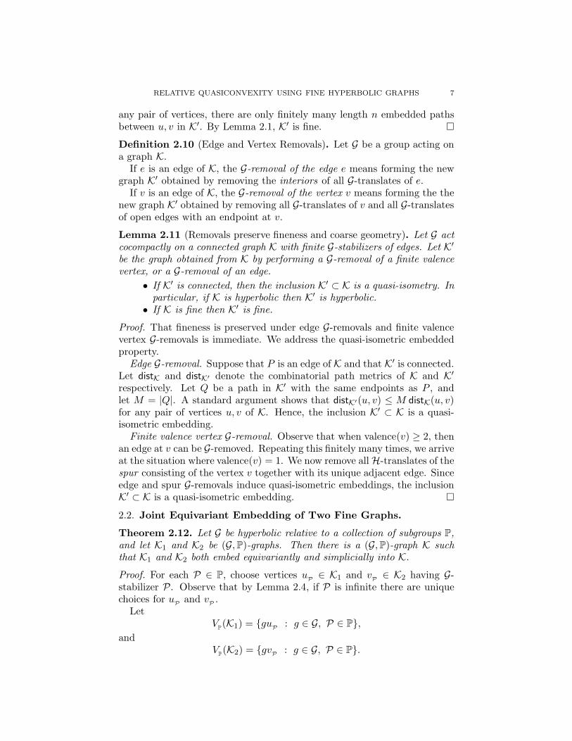
Definition 3.2 (Simple Ladder). A simple ladder between P and Q is a non-singular disc diagram D that is the union of a sequence of 2-cells R1, . . . , Rℓ

such that each Ri intersects P and Q in a nontrivial boundary arc, and


Figure 1. A simple ladder between two paths.

Ri ∩Rj is a nontrivial internal arc when |i− j| = 1, and Ri ∩Rj = ∅ when|i− j| > 1, finally the startpoint of P,Q lies in the interior of R1 ∩ ∂D, andthe endpoint of P,Q lies in the interior of Rℓ ∩ ∂D. See Figure 1.

Definition 3.3 (Quasigeodesic). Let K be a graph and let distK be theinduced length metric when all edges have length 1. For real constants λ ≥1, ǫ ≥ 0, a combinatorial path P is a (λ, ǫ)-quasigeodesic if for each subpathP ′ of P between vertices u and v, the length |P ′| is at most λ distK(u, v)+ ǫ.A (λ, 0)-quasigeodesic is called a λ-quasigeodesic.

Proposition 3.4 (Simple Ladder). Let K be a δ-hyperbolic graph. For eachλ ≥ 1, there is an integer N = N(δ, λ) > 0 such that for all n > N thefollowing property holds:

If P and Q are embedded λ-quasigeodesics with the same startpoint andendpoint, and with no common interior points. Then there is an embeddeddisc diagram D → Xn(K) between P and Q such that D is a simple ladder.

For the proof of Proposition 3.4, we recall the following well-known fact,a proof of which can found in [2, Chapter III.H, Corollary 1.8].

Lemma 3.5 (Slim rectangles). Let K be a δ-hyperbolic graph. For anyλ ≥ 1 there exists a constant ǫ = ǫ(δ, λ) > 0 with the following property. IfP = P1P2P3P4 is a closed path such that each Pi is a λ-quasigeodesic, theneach vertex of P1 is contained in the ǫ-neighborhood of the set of vertices ofP2P3P4.

Lemma 3.6 (Fellow traveling). Let K be a δ-hyperbolic graph. Let P be anembedded λ-quasigeodesic, and let G be a geodesic, such that P,G have thesame startpoint and endpoint. Let ǫ = ǫ(δ, λ) of Lemma 3.5. Suppose G isthe concatenation G1G2 · · ·Gℓ of edge-paths such that:

10ǫ ≤ |Gi| ≤ 20ǫ.

For each i, let Si be a geodesic from the startpoint of Gi to P . Notice that|Si| ≤ ǫ and is an edge-path. For i < ℓ, let Pi be the subpath of P from theendpoint of Si to the endpoint of Si+1, and let Pℓ be the subpath of P fromthe endpoint of Sℓ to the endpoint of P .

Then Pi and Pj have at most one point in common when i 6= j. Conse-quently, P = P1P2 . . . Pℓ.

Proof. First, Si is an edge-path for each i since it starts and ends at 0-cellsand is embedded. Moreover, |Si| < ǫ for each i by Lemma 3.5, since PG−1


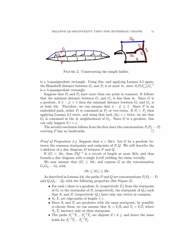
Figure 2. Constructing the simple ladder.

is a λ-quasigeodesic rectangle. Using this, and applying Lemma 3.5 again,the Hausdorff distance between Gi and Pi is at most 2ǫ, since SiPiS

−1i+1G

−1i

is a λ-quasigeodesic rectangle.Suppose that Pi and Pj have more than one point in common. It follows

that the minimal distance between Gi and Gj is less than 4ǫ. Since G isa geodesic, if |i − j| > 1 then the minimal distance between Gi and Gj isat least 10ǫ. Therefore, we can assume that |i − j| ≤ 1. Since P is anembedded path, either Pi is contained in Pj or vice-versa. If Pi ⊂ Pj thenapplying Lemma 3.5 twice, and using that each |Sk| < ǫ twice, we see thatGi is contained in the 4ǫ neighborhood of Gj . Since G is a geodesic, thiscan only happen if i = j.

The second conclusion follows from the first since the concatenation P1P2 · · ·Pℓ

covering P has no backtracks. �

Proof of Proposition 3.4. Suppose that n > 50ǫλ. Let G be a geodesic be-tween the common startpoints and endpoints of P,Q. We will describe the1-skeleton of a disc diagram D between P and Q.

If |G| < 10ǫ, then PQ−1 is a circuit of length at most 20λǫ and thusbounds a disc diagram with a single 2-cell yielding the claim trivially.

We now assume that |G| ≥ 10ǫ, and express G as the concatenationG1G2 · · ·Gℓ with

10ǫ ≤ |Gi| ≤ 20ǫ.

As described in Lemma 3.6, the paths P andQ are concatenations P1P2 · · ·Pℓ

and Q1Q2 · · ·Qℓ with the following properties (See Figure 2):

• For each i there is a geodesic Si (respectively Ti) from the startpointof Gi to the startpoint of Pi (respectively, the startpoint of Qi) suchthat Si and Pi (respectively Qi) have only one vertex in common.

• Si, Ti are edge-paths of length ≤ ǫ.• Since Si and Ti are geodesics with the same startpoint, by possiblyre-choose them, we can assume that Si = ViSi and Ti = ViTi whereSi, Ti intersect only at their startpoint.

• The paths S−1i Ti , S−1

j Tj are disjoint if i 6= j, and hence the same

holds for S−1i Ti , S−1

j Tj .


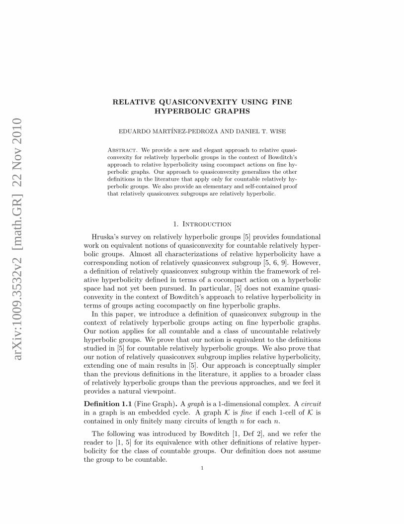
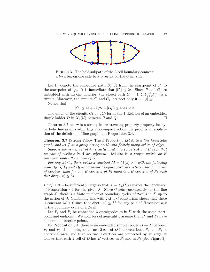
Figure 3. The bold subpath of the 2-cell boundary connectsa b-vertex on one side to a b-vertex on the other side.

Let Ui denote the embedded path S−1i Ti from the startpoint of Pi to

the startpoint of Qi. It is immediate that |Ui| ≤ 2ǫ. Since P and Q areembedded with disjoint interior, the closed path Ci = UiQiU

−1i+1P

−1i is a

circuit. Moreover, the circuits Ci and Cj intersect only if |i− j| ≤ 1.Notice that

|Ci| ≤ 4ǫ+ 2λ(2ǫ + |Gi|) ≤ 48ǫλ < n.

The union of the circuits C1, . . . , Cℓ forms the 1-skeleton of an embeddedsimple ladder D in Xn(K) between P and Q. �

Theorem 3.7 below is a strong fellow traveling property property for hy-perbolic fine graphs admitting a cocompact action. Its proof is an applica-tion of the definition of fine graph and Proposition 3.4.

Theorem 3.7 (Strong Fellow Travel Property). Let K be a fine hyperbolicgraph, and let G be a group acting on K with finitely many orbits of edges.

Suppose the vertex set of K is partitioned into subsets A and B such thatno pair of vertices in A are adjacent. Let dist be a proper metric on B

invariant under the action of G.For any λ ≥ 1, there exists a constant M = M(λ) > 0 with the following

property. If P1 and P2 are embedded λ-quasigeodesics between the same pairof vertices, then for any B-vertex u of P1 there is a B-vertex v of P2 suchthat dist(u, v) ≤ M .

Proof. Let n be sufficiently large so that X = Xn(K) satisfies the conclusionof Proposition 3.4 for the given λ. Since G acts cocompactly on the finegraph K, there is a finite number of boundary cycles of 2-cells in X up tothe action of G. Combining this with dist is G-equivariant shows that thereis constant M > 0 such that dist(u, v) ≤ M for any pair of B-vertices u, v

in the boundary cycle of a 2-cell.Let P1 and P2 be embedded λ-quasigeodesics in K with the same start-

point and endpoint. Without loss of generality, assume that P1 and P2 haveno common interior points.

By Proposition 3.4, there is an embedded simple ladder D → X betweenP1 and P2. Combining that each 2-cell of D intersects both P1 and P2 innontrivial arcs, and that no two A-vertices are connected by an edge, itfollows that each 2-cell of D has B-vertices in P1 and in P2 (See Figure 3).


Since each B-vertex of P1 belongs to a 2-cell of D, it follows that for anyB-vertex u of P1 there is a B-vertex v of P2 such that dist(u, v) ≤ M . �

4. Equivalences of Formulations of Relative quasiconvexity

In this section we prove Theorem 1.7 on the equivalence between relativequasiconvexity of Definition 1.3, labelled by (Q-0), and relative quasiconvex-ity of Definition 1.6, labelled by (Q-1), in the context of countable relativelyhyperbolic groups.

The argument introduces two auxiliary definitions of relative quasicon-

vexity, labelled by Q-1 and Q-0, and then the theorem follows after provingthe following equivalences:

(1) Q-1 ⇐⇒ Q-1 ⇐⇒ Q-0 ⇐⇒ Q-0.

The section is divided in six short parts as follows. First we recall thenotion of coned-off Cayley graph, and deduce a strong version of the fellowtravel property using the main result of Section 3. The second part showsthat relative quasiconvexity of Definition 1.6, labelled by (Q-1), implies fi-nite relative generation. The third part state the two auxiliary definitions.The remaining three parts correspond to each of the three equivalences inillustration (1).

For the rest of the section, let G be a hyperbolic group relative to acollection of subgroups P, let S be a finite relative generating set for (G,P),and let dist be a proper left-invariant metric on G.

4.1. The Coned-off Cayley Graph.

Definition 4.1 (Cayley Graph). Let S be a subset of a group G, and assumethat S is closed under inverses. The Cayley graph Γ(G, S) is an orientedlabelled 1-complex with vertex set G and edge set G × S. An edge (g, s)goes from the vertex g to the vertex gs and has label s. Observe that Γ(G, S)is connected if and only if S is a generating set of G.

The notion of coned-off Cayley graph is originally due to Farb [4] and thefollowing generalization is taking from [5, Sec. 3.4].

Definition 4.2 (Coned-off Cayley Graph Γ). Let S be a finite relativegenerating set for (G,P) and assume that S is closed under inverses. The

coned-off Cayley graph Γ(G,P, S) is the graph constructed from the Cayleygraph Γ = Γ(G, S) as follows: For each left coset gP with g ∈ G and P ∈ P,add a new vertex v(gP) to Γ, and add a 1-cell from this new vertex to each

element of gP. These new vertices of Γ(G,P, S) that are not in Γ are called

cone-vertices. Each 1-cell of Γ(G,P, S) between an element of G and a cone

vertex is a cone-edge. Note that the coned-off Cayley graph Γ(G,P, S) isconnected since S is a relative generating set for (G,P).

There is a related (genuine) Cayley graph of G with respect to the generat-ing set defined as the disjoint union S⊔

⊔i Pi which we denote by Γ(G, S∪P).


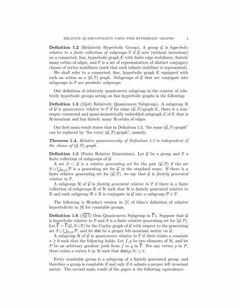
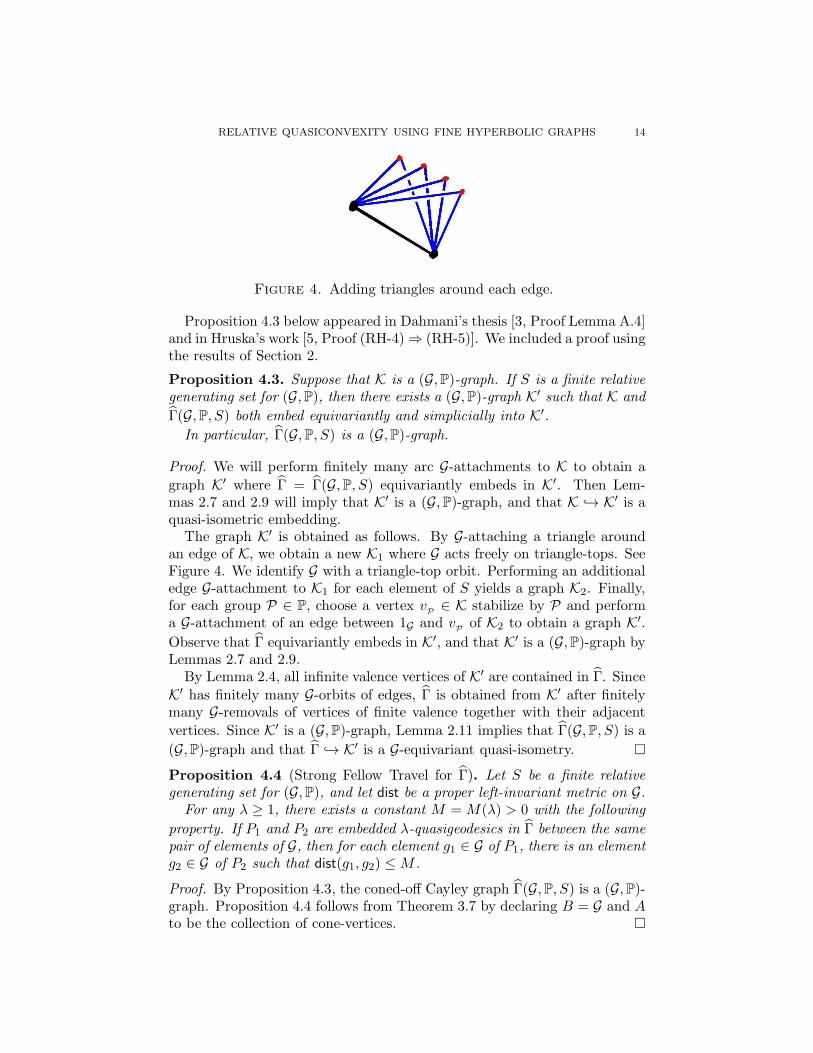
Figure 4. Adding triangles around each edge.

Proposition 4.3 below appeared in Dahmani’s thesis [3, Proof Lemma A.4]and in Hruska’s work [5, Proof (RH-4)⇒ (RH-5)]. We included a proof usingthe results of Section 2.

Proposition 4.3. Suppose that K is a (G,P)-graph. If S is a finite relativegenerating set for (G,P), then there exists a (G,P)-graph K′ such that K and

Γ(G,P, S) both embed equivariantly and simplicially into K′.

In particular, Γ(G,P, S) is a (G,P)-graph.

Proof. We will perform finitely many arc G-attachments to K to obtain a

graph K′ where Γ = Γ(G,P, S) equivariantly embeds in K′. Then Lem-mas 2.7 and 2.9 will imply that K′ is a (G,P)-graph, and that K → K′ is aquasi-isometric embedding.

The graph K′ is obtained as follows. By G-attaching a triangle aroundan edge of K, we obtain a new K1 where G acts freely on triangle-tops. SeeFigure 4. We identify G with a triangle-top orbit. Performing an additionaledge G-attachment to K1 for each element of S yields a graph K2. Finally,for each group P ∈ P, choose a vertex v

P∈ K stabilize by P and perform

a G-attachment of an edge between 1G and vPof K2 to obtain a graph K′.

Observe that Γ equivariantly embeds in K′, and that K′ is a (G,P)-graph byLemmas 2.7 and 2.9.

By Lemma 2.4, all infinite valence vertices of K′ are contained in Γ. Since

K′ has finitely many G-orbits of edges, Γ is obtained from K′ after finitelymany G-removals of vertices of finite valence together with their adjacent

vertices. Since K′ is a (G,P)-graph, Lemma 2.11 implies that Γ(G,P, S) is a

(G,P)-graph and that Γ → K′ is a G-equivariant quasi-isometry. �

Proposition 4.4 (Strong Fellow Travel for Γ). Let S be a finite relativegenerating set for (G,P), and let dist be a proper left-invariant metric on G.

For any λ ≥ 1, there exists a constant M = M(λ) > 0 with the following

property. If P1 and P2 are embedded λ-quasigeodesics in Γ between the samepair of elements of G, then for each element g1 ∈ G of P1, there is an elementg2 ∈ G of P2 such that dist(g1, g2) ≤ M .

Proof. By Proposition 4.3, the coned-off Cayley graph Γ(G,P, S) is a (G,P)-graph. Proposition 4.4 follows from Theorem 3.7 by declaring B = G and A

to be the collection of cone-vertices. �


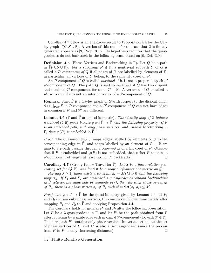
Corollary 4.7 below is an analogous result to Proposition 4.4 for the Cay-ley graph Γ(G, S ∪ P). A version of this result for the case that G is finitelygenerated appears as [9, Prop. 3.15]. Its hypothesis requires that the quasi-geodesics do not backtrack in the following sense based on [9, Def. 3.9]:

Definition 4.5 (Phase Vertices and Backtracking in Γ). Let Q be a pathin Γ(G, S ∪ P). For a subgroup P ∈ P, a nontrivial subpath U of Q iscalled a P-component of Q if all edges of U are labelled by elements of P,in particular, all vertices of U belong to the same left coset of P.

An P-component of Q is called maximal if it is not a proper subpath ofP-component of Q. The path Q is said to backtrack if Q has two disjointand maximal P-components for some P ∈ P. A vertex v of Q is called aphase vertex if v is not an interior vertex of a P-component of Q.

Remark. Since Γ is a Cayley graph of G with respect to the disjoint unionS ⊔

⊔P∈P P, a P-component and a P ′-component of Q can not have edges

in common if P and P ′ are different.

Lemma 4.6 (Γ and Γ are quasi-isometric). The identity map of G induces

a natural (2, 0)-quasi-isometry ϕ : Γ → Γ with the following property. If Pis an embedded path, with only phase vertices, and without backtracking in

Γ, then ϕ(P ) is embedded in Γ.

Proof. The quasi-isometry ϕ maps edges labelled by elements of S to the

corresponding edge in Γ, and edges labelled by an element of P ∈ P aremap to a 2-path passing through a cone-vertex of a left coset of P. Observethat if P is embedded and ϕ(P ) is not embedded, then either P contains aP-component of length at least two, or P backtracks. �

Corollary 4.7 (Strong Fellow Travel for Γ). Let S be a finite relative gen-erating set for (G,P), and let dist be a proper left-invariant metric on G.

For any λ ≥ 1, there exists a constant M = M(λ) > 0 with the followingproperty. If P1 and P2 are embedded λ-quasigeodesics without backtrackingin Γ between the same pair of elements of G, then for each phase vertex g1of P1, there is a phase vertex g2 of P2 such that dist(g1, g2) ≤ M .

Proof. Let ϕ : Γ → Γ be the quasi-isometry given by Lemma 4.6. If P1

and P2 contain only phase vertices, the conclusion follows immediately after

mapping P1 and P2 to Γ and applying Proposition 4.4.The Corollary holds for general P1 and P2 after the following observation.

Let P be a λ-quasigeodesic in Γ, and let P ′ be the path obtained from P

after replacing by a single edge each maximal P-component (for each P ∈ P).The new path P ′ contains only phase vertices, its vertex set equals the setof phase vertices of P , and P ′ is also a λ-quasigeodesic (since the processfrom P to P ′ is only shortening distances). �

4.2. Finite Relative Generation.


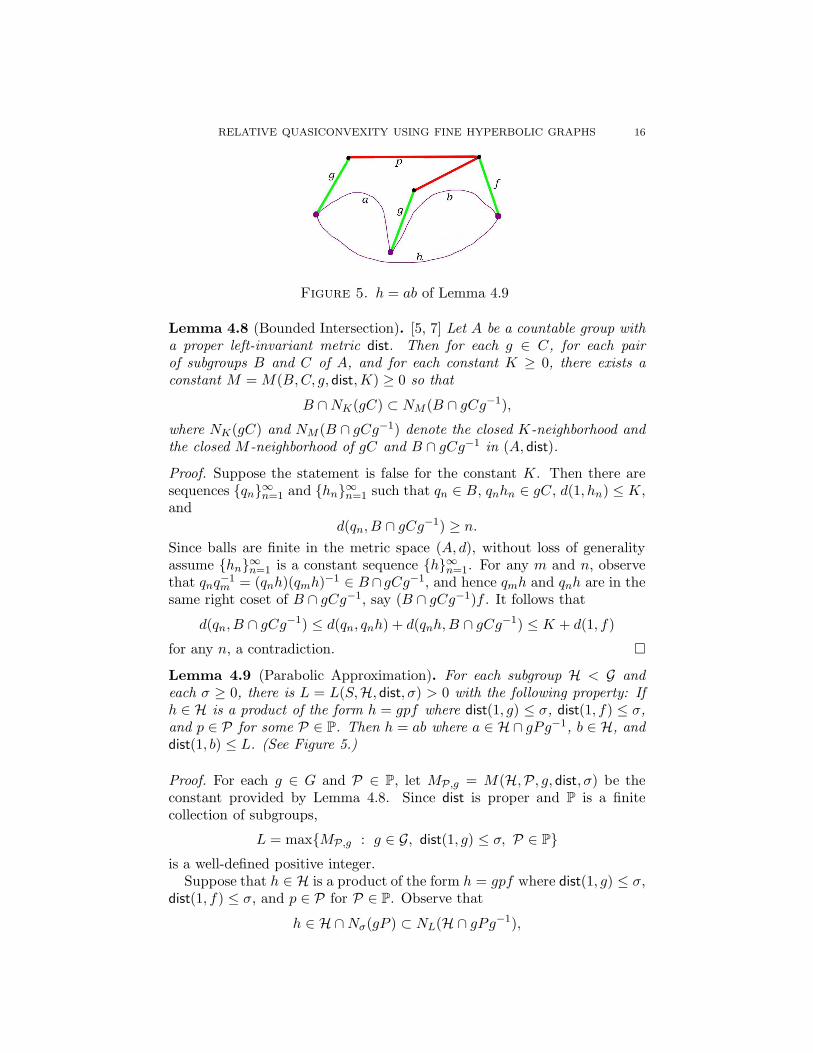
Figure 5. h = ab of Lemma 4.9

Lemma 4.8 (Bounded Intersection). [5, 7] Let A be a countable group witha proper left-invariant metric dist. Then for each g ∈ C, for each pairof subgroups B and C of A, and for each constant K ≥ 0, there exists aconstant M = M(B,C, g, dist,K) ≥ 0 so that

B ∩NK(gC) ⊂ NM (B ∩ gCg−1),

where NK(gC) and NM (B ∩ gCg−1) denote the closed K-neighborhood andthe closed M -neighborhood of gC and B ∩ gCg−1 in (A, dist).

Proof. Suppose the statement is false for the constant K. Then there aresequences {qn}

∞n=1 and {hn}

∞n=1 such that qn ∈ B, qnhn ∈ gC, d(1, hn) ≤ K,

and

d(qn, B ∩ gCg−1) ≥ n.

Since balls are finite in the metric space (A, d), without loss of generalityassume {hn}

∞n=1 is a constant sequence {h}∞n=1. For any m and n, observe

that qnq−1m = (qnh)(qmh)−1 ∈ B∩ gCg−1, and hence qmh and qnh are in the

same right coset of B ∩ gCg−1, say (B ∩ gCg−1)f . It follows that

d(qn, B ∩ gCg−1) ≤ d(qn, qnh) + d(qnh,B ∩ gCg−1) ≤ K + d(1, f)

for any n, a contradiction. �

Lemma 4.9 (Parabolic Approximation). For each subgroup H < G andeach σ ≥ 0, there is L = L(S,H, dist, σ) > 0 with the following property: Ifh ∈ H is a product of the form h = gpf where dist(1, g) ≤ σ, dist(1, f) ≤ σ,and p ∈ P for some P ∈ P. Then h = ab where a ∈ H ∩ gPg−1, b ∈ H, anddist(1, b) ≤ L. (See Figure 5.)

Proof. For each g ∈ G and P ∈ P, let MP,g = M(H,P, g, dist, σ) be theconstant provided by Lemma 4.8. Since dist is proper and P is a finitecollection of subgroups,

L = max{MP,g : g ∈ G, dist(1, g) ≤ σ, P ∈ P}

is a well-defined positive integer.Suppose that h ∈ H is a product of the form h = gpf where dist(1, g) ≤ σ,

dist(1, f) ≤ σ, and p ∈ P for P ∈ P. Observe that

h ∈ H ∩Nσ(gP ) ⊂ NL(H ∩ gPg−1),


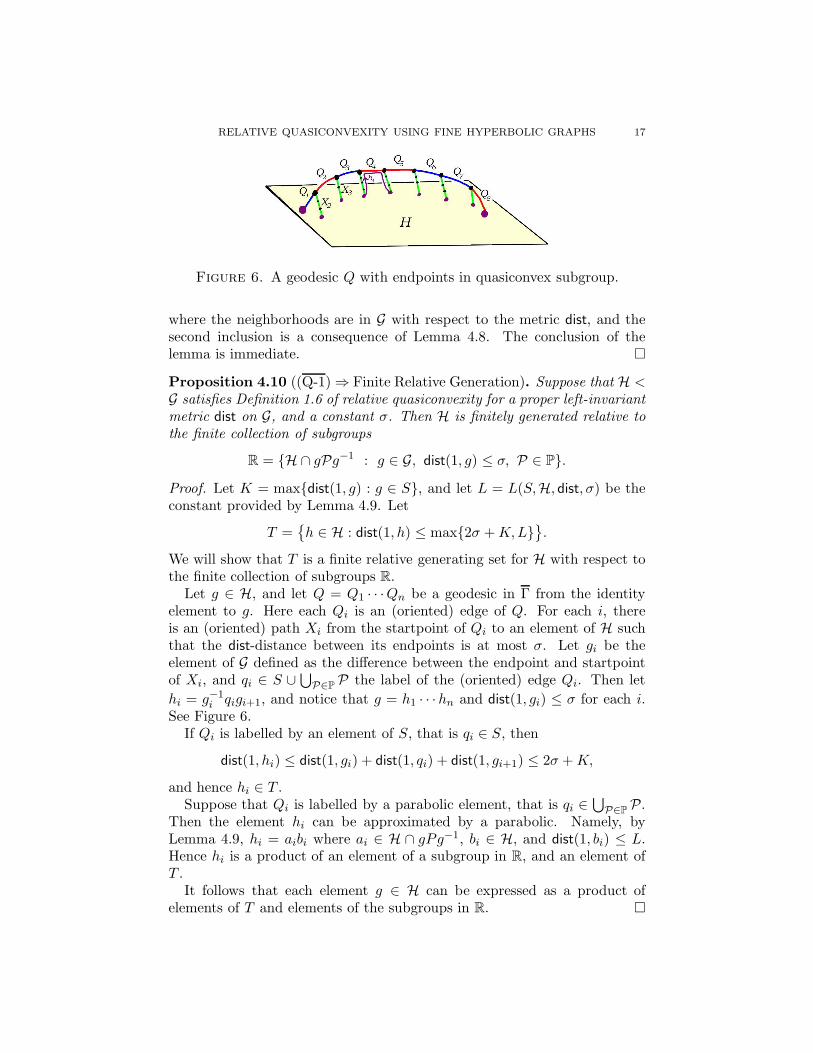
Figure 6. A geodesic Q with endpoints in quasiconvex subgroup.

where the neighborhoods are in G with respect to the metric dist, and thesecond inclusion is a consequence of Lemma 4.8. The conclusion of thelemma is immediate. �

Proposition 4.10 ((Q-1) ⇒ Finite Relative Generation). Suppose that H <

G satisfies Definition 1.6 of relative quasiconvexity for a proper left-invariantmetric dist on G, and a constant σ. Then H is finitely generated relative tothe finite collection of subgroups

R = {H ∩ gPg−1 : g ∈ G, dist(1, g) ≤ σ, P ∈ P}.

Proof. Let K = max{dist(1, g) : g ∈ S}, and let L = L(S,H, dist, σ) be theconstant provided by Lemma 4.9. Let

T ={h ∈ H : dist(1, h) ≤ max{2σ +K,L}

}.

We will show that T is a finite relative generating set for H with respect tothe finite collection of subgroups R.

Let g ∈ H, and let Q = Q1 · · ·Qn be a geodesic in Γ from the identityelement to g. Here each Qi is an (oriented) edge of Q. For each i, thereis an (oriented) path Xi from the startpoint of Qi to an element of H suchthat the dist-distance between its endpoints is at most σ. Let gi be theelement of G defined as the difference between the endpoint and startpointof Xi, and qi ∈ S ∪

⋃P∈P P the label of the (oriented) edge Qi. Then let

hi = g−1i qigi+1, and notice that g = h1 · · · hn and dist(1, gi) ≤ σ for each i.

See Figure 6.If Qi is labelled by an element of S, that is qi ∈ S, then

dist(1, hi) ≤ dist(1, gi) + dist(1, qi) + dist(1, gi+1) ≤ 2σ +K,

and hence hi ∈ T .Suppose that Qi is labelled by a parabolic element, that is qi ∈

⋃P∈PP.

Then the element hi can be approximated by a parabolic. Namely, byLemma 4.9, hi = aibi where ai ∈ H ∩ gPg−1, bi ∈ H, and dist(1, bi) ≤ L.Hence hi is a product of an element of a subgroup in R, and an element ofT .

It follows that each element g ∈ H can be expressed as a product ofelements of T and elements of the subgroups in R. �


4.3. Auxiliary Definitions. Since G acts on the connected graph K withfinitely many orbits of edges, an standard argument shows that G is finitelygenerated relative to P. This justifies the existence of finite relative gener-ating sets in the following two definitions.

Definition 4.11 ((Q-1) Auxiliary definition in Γ). Let S be a finite relativegenerating set for (G,P), and let dist be a proper left-invariant metric onG. A subgroup H of G is quasiconvex relative to P if there exists a constantσ ≥ 0 such that the following holds: Let f , g be two elements of H, and let

P be an arbitrary geodesic path from f to g in Γ(G,P, S). For any non-conevertex p of P , there exists a non-cone vertex h in H such that dist(p, h) ≤ σ.

Definition 4.12 ((Q-0) Second auxiliary definition in Γ). Let S be a finiterelative generating set for (G,P). A subgroup H of G is quasiconvex relative

to P if there is a non-empty connected H-invariant subgraph L of Γ that isquasi-isometrically embedded and has finitely many H-orbits of edges.

4.4. The equivalence (Q-1) ⇔ (Q-1).

Proposition 4.13 ((Q-1) ⇔ (Q-1)). Relative quasiconvexity of Defini-tion 1.6 and relative quasiconvexity of Definition 4.11 are equivalent notions.

In particular, Definition 4.11 is independent of the generating set S andthe left-invariant metric dist on G.

Proof. Let ϕ : Γ → Γ be the natural quasi-isometry induced by the identitymap on G, see Lemma 4.6.

Suppose that H < G satisfies Definition 4.11 for a constant σ. Let P be ageodesic in Γ between elements of H. Then ϕ maps P to a 2-quasigeodesic

P . Let Q be a geodesic in Γ between the endpoints of P . By Proposition 4.4,

there is a constant M = M(2) such that for each non-cone vertex p of P ,

there is a non-cone vertex q ∈ Q such that dist(p, q) ≤ M . By Definition 4.11,

for each non-cone vertex q of Q, there is h ∈ H such that dist(q, h) ≤ σ.

Since the vertices of P map to the non-cone vertices of P , it follows that foreach vertex p of P , there is a vertex h of H such that dist(p, h) ≤ σ + M .Therefore, H satisfies Definition 1.6.

Conversely, suppose that H < G satisfies Definition 1.6 for a constant σ,

and let P be a geodesic in Γ between elements of H. Let Q be a geodesicin Γ between the endpoints of P . Observe that there is an embedded 2-quasigeodesic P in Γ that maps onto P by ϕ, has only phase vertices, anddoes not backtrack. Then Proposition 4.7 implies that there is a constantM = M(2) such that the vertices of Q and P (and hence P ) are M -closedwith respect to the metric dist. Since the vertices of Q are σ-close to the ele-ments of H with respect to dist, we conclude that H satisfies Definition 4.11for the constant σ +M . �



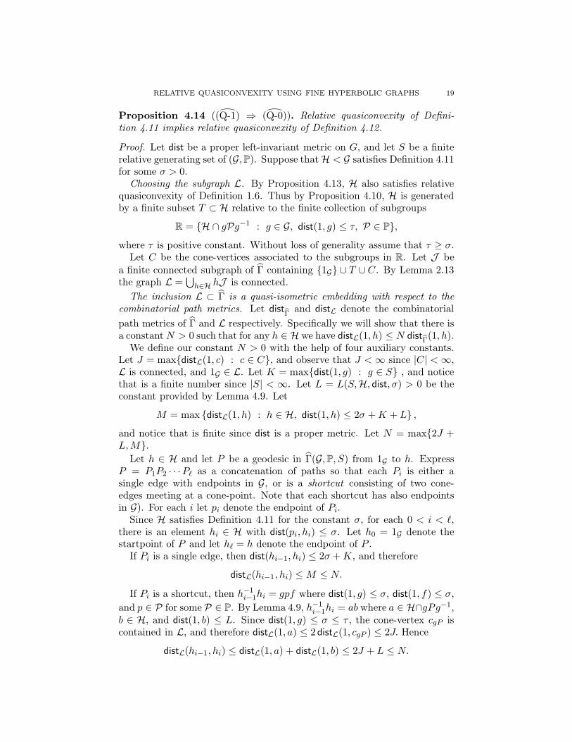
Proposition 4.14 ((Q-1) ⇒ (Q-0)). Relative quasiconvexity of Defini-tion 4.11 implies relative quasiconvexity of Definition 4.12.

Proof. Let dist be a proper left-invariant metric on G, and let S be a finiterelative generating set of (G,P). Suppose thatH < G satisfies Definition 4.11for some σ > 0.

Choosing the subgraph L. By Proposition 4.13, H also satisfies relativequasiconvexity of Definition 1.6. Thus by Proposition 4.10, H is generatedby a finite subset T ⊂ H relative to the finite collection of subgroups

R = {H ∩ gPg−1 : g ∈ G, dist(1, g) ≤ τ, P ∈ P},

where τ is positive constant. Without loss of generality assume that τ ≥ σ.Let C be the cone-vertices associated to the subgroups in R. Let J be

a finite connected subgraph of Γ containing {1G} ∪ T ∪ C. By Lemma 2.13the graph L =

⋃h∈H hJ is connected.

The inclusion L ⊂ Γ is a quasi-isometric embedding with respect to thecombinatorial path metrics. Let dist

Γand distL denote the combinatorial

path metrics of Γ and L respectively. Specifically we will show that there isa constantN > 0 such that for any h ∈ H we have distL(1, h) ≤ N dist

Γ(1, h).

We define our constant N > 0 with the help of four auxiliary constants.Let J = max{distL(1, c) : c ∈ C}, and observe that J < ∞ since |C| < ∞,L is connected, and 1G ∈ L. Let K = max{dist(1, g) : g ∈ S} , and noticethat is a finite number since |S| < ∞. Let L = L(S,H, dist, σ) > 0 be theconstant provided by Lemma 4.9. Let

M = max {distL(1, h) : h ∈ H, dist(1, h) ≤ 2σ +K + L} ,

and notice that is finite since dist is a proper metric. Let N = max{2J +L,M}.

Let h ∈ H and let P be a geodesic in Γ(G,P, S) from 1G to h. ExpressP = P1P2 · · ·Pℓ as a concatenation of paths so that each Pi is either asingle edge with endpoints in G, or is a shortcut consisting of two cone-edges meeting at a cone-point. Note that each shortcut has also endpointsin G). For each i let pi denote the endpoint of Pi.

Since H satisfies Definition 4.11 for the constant σ, for each 0 < i < ℓ,there is an element hi ∈ H with dist(pi, hi) ≤ σ. Let h0 = 1G denote thestartpoint of P and let hℓ = h denote the endpoint of P .

If Pi is a single edge, then dist(hi−1, hi) ≤ 2σ +K, and therefore

distL(hi−1, hi) ≤ M ≤ N.

If Pi is a shortcut, then h−1i−1hi = gpf where dist(1, g) ≤ σ, dist(1, f) ≤ σ,

and p ∈ P for some P ∈ P. By Lemma 4.9, h−1i−1hi = ab where a ∈ H∩gPg−1,

b ∈ H, and dist(1, b) ≤ L. Since dist(1, g) ≤ σ ≤ τ , the cone-vertex cgP iscontained in L, and therefore distL(1, a) ≤ 2 distL(1, cgP ) ≤ 2J. Hence

distL(hi−1, hi) ≤ distL(1, a) + distL(1, b) ≤ 2J + L ≤ N.


To conclude, observe that

distL(1, h) ≤ℓ∑

i=1

distL(hi−1, hi) ≤ Nℓ ≤ N distΓ(1, h). �

Proposition 4.15 ((Q-0) ⇒ (Q-1)). Relative quasiconvexity of Defini-tion 4.12 implies relative quasiconvexity of Definition 4.11.

Proof. Let dist be a proper left-invariant metric on G, and let S be a fi-nite relative generating set of (G,P). Suppose that H < G satisfies Defini-tion 4.12.

Let L be connected quasi-isometrically embedded subgraph L of Γ =

Γ(G,P, S) that is H-equivariant and has finitely many H-orbits of edges.The following statements about L hold.

(1) Since L is connected, it has at least one vertex that is not a cone-vertex. Without loss of generality, assume that the identity 1G ∈ Gis a vertex of L. In particular, we assume that all elements of H arevertices of L.

(2) Since H acts cocompactly on L, there is κ > 0 such that each vertexof L is either a cone-vertex, or an element of G is at distance at mostκ from H with respect to dist.

(3) Since L is quasi-isometrically embedded subgraph of Γ, there is λ ≥ 1

such that any geodesic in L is a λ-quasi-geodesic in Γ.

Let M = M(λ) > 0 be the constant provided by Proposition 4.4. Let Q

be a geodesic in Γ with endpoints in H. Let P be a geodesic in L betweenthe endpoints of Q. By Statement (3), P is a λ-quasigeodesic. Therefore,Proposition 4.4 implies that for each non-cone vertex q of Q, there is anon-cone vertex p of P such that dist(p, q) ≤ M . Combining this withStatement (2) shows that for each non-cone vertex q of Q there is a non-cone vertex h ∈ H such that dist(p, h) ≤ M + κ. Therefore, H satisfiesDefinition 4.11. �


Proposition 4.16 ((Q-0) ⇔ (Q-0)). Relative quasiconvexity of Defini-tion 4.12 is equivalent to relative quasiconvexity of Definition 1.3.

Proof. By Proposition 4.3, the coned-off Cayley graph Γ(G,P, S) with re-spect to a finite relative generating set S is a (G,P)-graph. By Theorem 2.14,a subgroup H satisfies relative quasiconvexity of Definition 1.3 for a (G,P)-

graph K if and only if it does for Γ(G,P, S). �

References

[1] B.H. Bowditch. Relatively hyperbolic groups. preprint, 1999.[2] Martin R. Bridson and Andre Haefliger. Metric spaces of non-positive curvature, vol-

ume 319 of Grundlehren der Mathematischen Wissenschaften [Fundamental Princi-ples of Mathematical Sciences]. Springer-Verlag, Berlin, 1999.


[3] F. Dahmani. Les groupes relativement hyperboliques et leurs bords. PhD thesis, Univ.Louis Pasteur, Strasbourg, France, 2003.

[4] B. Farb. Relatively hyperbolic groups. GAFA, Geom. funct. anal., 8(5):810–840, 1998.[5] G. Christopher Hruska. Relative hyperbolicity and relative quasiconvexity for count-

able groups. Algebr. Geom. Topol., 10(3):1807–1856, 2010.[6] Jason Fox Manning and Eduardo Martınez-Pedroza. Separation of relatively quasi-

convex subgroups. Pacific J. Math., 244(2):309–334, 2010.[7] Eduardo Martınez-Pedroza. Combination of quasiconvex subgroups of relatively hy-

perbolic groups. Groups Geom. Dyn., 3(2):317–342, 2009.[8] Eduardo Martınez-Pedroza and Daniel T. Wise. Local quasiconvexity of groups act-

ing on small cancellation complexes. J. Pure Appl. Algebra., to appear. Preprint atarXiv:1009.3407.

[9] Denis V. Osin. Relatively hyperbolic groups: intrinsic geometry, algebraic properties,and algorithmic problems. Mem. Amer. Math. Soc., 179(843):vi+100, 2006.

[10] Pekka Tukia. Conical limit points and uniform convergence groups. J. Reine Angew.Math., 501:71–98, 1998.

McMaster University, Hamilton, Ontario, Canada L8P 3E9

E-mail address: [email protected]

McGill University, Montreal, Quebec, Canada H3A 2K6

E-mail address: [email protected]

arXiv:1009.3407

Documents

RELATIVE QUASICONVEXITY USING FINE … QUASICONVEXITY USING FINE HYPERBOLIC GRAPHS 2 Deﬁnition 1.2 (Relatively Hyperbolic Group). A group G is hyperbolic relative to a ﬁnite collection