Relative Performance Benchmarks: Do Boards Get It Right?

Paul Ma Jee Eun Shin Charles C.Y. Wang

Working Paper 17-039

Working Paper 17-039

Copyright © 2016, 2017, 2018 by Paul Ma, Jee Eun Shin, and Charles C.Y. Wang

Working papers are in draft form. This working paper is distributed for purposes of comment and discussion only. It may not be reproduced without permission of the copyright holder. Copies of working papers are available from the author.

Relative Performance Benchmarks: Do Boards Follow the Informativeness Principle?

Paul Ma University of Minnesota

Jee Eun Shin Harvard Business School

Charles C.Y. Wang Harvard Business School

Relative Performance Benchmarks:Do Boards Follow the Informativeness Principle?∗

Paul MaUniversity of Minnesota

Carlson School of Management

Jee Eun ShinHarvard Business School

Charles C.Y. WangHarvard Business School

February 13th, 2018

Abstract

Relative total shareholder return (rTSR) is increasingly used to incentivize and evaluate managers.Although compensation experts acknowledge a primary objective is to filter shocks unrelated tomanagerial performance, we document that a significant subset of firms, who choose index-basedrTSR-benchmarks in lieu of specific peers, do not adequately achieve this objective. Structuralestimates reveal that noisy-benchmark selection implies significant negative performance conse-quences. Reduced-form analysis shows that a firm’s choice of index-based benchmarking is 1)driven by its compensation consultants’ systematic tendencies and governance-related frictions,and 2) associated with lower ROA, suggesting noisy-benchmark selection is a novel indicator ofweak governance.

JEL: G30, M12, M52Keywords: Empirical contract theory; executive compensation; relative TSR; common shockfiltration; career concerns; search-based peers; board of directors; corporate governance; compen-sation consultants

∗This paper was previously circulated under the title “Relative Performance Benchmarks: Do Boards Get it Right?”. Theauthors can be contacted at paulma@umn.edu, jeshin@hbs.edu, and charles.cy.wang@hbs.edu. We have benefited from adviceand suggestions from Hengjie Ai, Santiago Bazdresch, Alan Benson, Brian Cadman (discussant), Gerardo Perez Cavazos, ShaneDikolli (discussant), Vyacheslav Fos (discussant), Frank Gigler, Guojin Gong, Thomas Hemmer, Sudarshan Jayaraman, GeorgeJohn, Chandra Kanodia, Heedong Kim (discussant), David Larcker, Eva Liang, Melissa Martin, Kevin Murphy, Jonathan Nam,Gaizka Ormazabal (discussant), Xiaoxia Peng, Ruidi Shang, Matt Shaffer, John Shoven, Pervin Shroff, Martin Szydlowski, ChaoTang, Akhmed Umyarov, Felipe Varas, Martin Wu, Eric Yeung (discussant), Ivy Zhang and conference and seminar participantsat FARS, Georgia State University, Harvard Business School, HKUST Accounting Symposium, SMU Accounting Symposium,UBC Winter Finance Conference, University of Florida, the Utah Winter Accounting Conference, and the American AccountingAssociation Annual Meeting. We give thanks to Srikant Datar and Paula Price from Harvard Business School, Yulan Shen (Headof Executive Compensation) of Biogen, Barry Sullivan (Managing Director) of Semler Brossy, Terry Adamson (Partner), JonBurg (Partner), and Daniel Kapinos (Associate Partner) of Aon Hewitt, and to Nikhil Lele (Principal) and Trent Tishkowski(Principal) of Ernst and Young for clarifying institutional details and for helpful feedback. We also thank Kyle Thomas andRaaj Zutshi for outstanding research assistance. Paul Ma is grateful for research support from the University of MinnesotaAccounting Research Center and the Dean’s Small Research and Travel Grant. All errors remain our own.

Relative Performance Benchmarks 1

1 Introduction

The measurement of performance is a critical element in the design of managerial incentives. In the

standard principle-agent framework, the classic theoretical insight suggests that the principal—in practice,

the board—should evaluate managers’ performance using performance metrics that are informative about

managerial effort or talent (the “informativeness principle”) (Holmstrom, 1979; Shavell, 1979). In particular,

when a performance metric contains common noise that is beyond the CEO’s control, a measure of relative

performance that filters out such noise can be desirable. Furthermore, designing incentive contracts around

relative performance metrics should in theory help to elicit costly unobservable effort from risk-averse managers

and improve firm performance (Holmstrom, 1979, 1982).

Consistent with filtering common market- or industry-wide noise, market participants have increasingly

turned their attention to relative performance metrics to evaluate the performance of firms and their top

managers. Over the last ten years, relative total shareholder returns (rTSR)—that is, firm’s own TSR

relative to an index or group of peer firms—has become perhaps the single most widely used performance

metric by which companies and their executives are judged by market participants. Since 2006 the SEC has

required firms to disclose rTSR in their annual report to shareholders.2 The New York Stock Exchange’s

Listing Company Manual (Section 303A.05) recommends that compensation committee members consider a

firm’s rTSR in determining long-run executive incentives. The influential proxy advisory firm Institutional

Shareholder Services (ISS) relies on an analysis of the relationship between a firm’s rTSR and its executive’s

pay relative to peers to judge whether an executive’s compensation is justified by performance and to formulate

its say-on-pay recommendations. Activist investors often focus on poor rTSR as evidence of poor management

quality or performance.3 Finally, as part of its implementation of the 2010 Dodd-Frank Act, the SEC recently

proposed Rule No. 34-74835 requiring firms to disclose comparisons of executive compensation to that of

peers in terms of rTSR in annual proxy statements.

The growing preference for rTSR as a performance metric is also evident in the trend toward linking

rTSR to performance-based executive contracts. Data from ISS Incentive Labs—on approximately 1,500

of the largest firms in the stock market—suggest that the proportion of firms that explicitly link executive

performance contracts to relative performance metrics increased from around 20% in 2006 to nearly 50%

in 2014 (see Figure 1). Moreover, among firms that engage in explicit relative performance benchmarking,

2Under Regulation S-K Item 201(e), firms are obligated to publish rTSR based on an industry or line of business index, or onpeer firms selected in good faith based on line of business and/or firm size (see, e.g., https://www.law.cornell.edu/cfr/text/17/229.201).

3Brav, Jiang, Partnoy and Thomas (2008) documents activists’ targets having lower stock returns relative to industry peers.As a recent example, in its 2017 proxy fight against Proctor and Gamble management, Trian argued that the company’s directorshave performed poorly by referencing the company’s low TSR relative to the company’s peers over each director’s tenure.

Relative Performance Benchmarks 2

an increasing proportion (from about 70% in 2006 to nearly 90% in 2014) use rTSR as a metric to which

performance incentives are tied.

In our qualitative background research, all of the compensation experts we interviewed—including

compensation consultants as well as corporate directors and corporate managers responsible for assessing and

designing executive compensation—noted that filtering market- or industry-level noise from firm performance,

which is outside of managers’ control, is one of the primary objectives of rTSR, and a reason for its rising

popularity in executive compensation. Indeed, such a view also emerges from a narrative analysis of white

papers on rTSR (summarized in Table A.I), published by the leading compensation consultants capturing

approximately 90% of the market. For example, these white papers noted that rTSR “levels the playing

field” in measuring managerial performance by taking into account the “macroeconomic and other market

factors affecting the business.” In doing so, rTSR “supports shareholder alignment,” by “align[ing] executive

wealth with the shareholder experience.” Put differently, rTSR is attractive to the extent it isolates the firm’s

“alpha”: its performance relative to an appropriate investment benchmark (i.e., the common component of a

firm’s TSR).4

Despite the appeal of rTSR, a central challenge to its application resides in the selection of peers to

measure and filter the common or exogenous component of performance—i.e., the extent to which it follows

the informativeness principle.5 The quality of such a relative performance measure can be crucial through its

impact on managerial effort provision, to the extent that managerial incentives are tied to such measures,

either explicitly via performance-based contracts or implicitly because shareholders’, board of directors’, and

the executive labor market’ assessment of the CEO’s reputation or talent depend on relative performance.6

This paper examines the degree to which firms’ selection of peers for rTSR is consistent with the

informativeness principle. We focus on the sample of firms that explicitly tie executive compensation to rTSR,

for whom the quality or the informativeness of rTSR are expected to be of greater importance. For example,

in addition to the increasing prevalence of rTSR-based pay, our back-of-the-envelope estimates suggest that

rTSR-based incentives have an economically important and increasing impact on CEO compensation. Between

2006 and 2014, on average 73% of the relative-performance target payouts are accounted for by rTSR-based

payouts; moreover, meeting rTSR targets increases the CEO’s incentive-plan-based compensation (assuming

4Note that the concept of removing common noise and shareholder alignment are one and the same. Without loss of generality,under a linear one-factor structure, p = a+ c+ e, where p is returns, c is the common component of returns, and e is idiosyncraticnoise in returns, relative returns (p− c) is equivalent to the excess returns of the firm (a+ e), i.e., the manager’s “alpha”.

5For example, Barry Sullivan, managing director of the compensation consulting firm Semler Brossy, described relativeperformance measurement as “seductive in theory” at the 2014 National Association of Corporate Directors Leading Minds ofCompensation Conference. But, he continued, “The challenge is in practice, do we really have a peer group that we feel goodmeasuring? If not, do we then have to extend to a broader market index, and if we do that, are we stepping too far away fromour core business or are we introducing some noise around the relative TSR construct?”

6See, for example, Holmstrom (1999); Avery, Chevalier and Schaefer (1998); Brickley, Linck and Coles (1999); Hayes andSchaefer (2000); Murdock (2002); Fee and Hadlock (2003); Milbourn (2003); Horner and Lambert (2016); Focke, Maug andNiessen-Ruenzi (2017); Chattopadhyay, Shaffer and Wang (2017).

Relative Performance Benchmarks 3

that all other performance-based targets are met) by an average of 40%.

We examine to what extent these firms’ chosen relative performance benchmarks explain the firms’ stock

returns, relative to a normative benchmark. To contextualize our empirical findings, we also frame the

analysis in terms of the classic principal-agent model of Holmstrom and Milgrom (1987), which predicts that

benchmarks will be optimally chosen to filter out the common component of performance. Drawing on this

framework, we then analyze and quantify the theoretical implications of relative performance benchmarks’

inefficacy at eliminating common noise for firm performance, absent frictions in peer selection. Finally, we

examine potential sources of friction and alternative theories and economic factors that could explain why

certain firms’ benchmarks do not appear to adequately capture common shocks in firm performance (that is,

to adhere to the informativeness principle).

We document four main findings. Our first set of analyses compares the performance of firms’ disclosed

peer benchmarks, to that of a normative relative performance benchmark in terms of their ability to explain

the variation in own-firm returns. We initially use search-based peers (SBPs), a set of economically-related

peer firms identified by investors’ searches on the SEC’s EDGAR platform. Lee, Ma and Wang (2015) and

Lee, Ma and Wang (2016) show that SBPs are superior to other state-of-the-art peer identification schemes at

explaining variations in firms’ stock returns, valuation multiples, and fundamental performance characteristics.

We find that firms’ disclosed benchmarks perform significantly worse at explaining the co-movement of stock

returns. This underperformance is concentrated in the set of firms that choose index-based benchmarks;

firms that choose specific peers perform only modestly worse. Compared to a portfolio of top 10 SBPs, firms’

disclosed index-based benchmarks explain 14% less of the time-series variation in their out-of-sample monthly

stock returns (i.e., time-series regression R2); comparable underperformance is merely 2.3% for firms using

specific peers.

These findings are not unique to the choice of SBPs as the normative benchmark. As an alternative,

we use firms’ chosen compensation benchmarking peers as the normative benchmark and find very similar

results. Together, these findings raise questions about the appropriateness of choosing indexes—effectively

benchmarking to a large number of peers—in lieu of a narrower but potentially more relevant peer set that is

already available, e.g., firms’ own compensation benchmarking peers or search-based peers (Lewellen and

Metrick, 2010; Lee, Ma and Wang, 2015).

Our second set of findings interpret these performance differences in R2 in the context of a standard

principal-agent framework absent any frictions in peer selection. We show that poorer selection of benchmarks

(larger measurement error variances) implies lower efficacy at filtering out common shocks and leads to poorer

incentives for managers. For any set of performance benchmark, this framework enables us to structurally

estimate the variance of the measurement error up to a scalar constant. Consistent with the time-series R2

Relative Performance Benchmarks 4

results, our estimates suggest that firms’ chosen index-based benchmarks yield measurement error variances

that are at least 16% higher than SBPs, whereas specific-peer-based benchmarks exhibit measurement error

variances that are at least 4.4% higher.

More importantly, our structural estimates suggest that, in the absence of frictions from selecting a precise

set of peers, the measurement error variances of firms’ chosen performance benchmarks reduce managerial

effort and result in an on-average performance penalty of 60 to 153 basis points in annual stock returns,

using plausible ranges of risk aversion. These magnitudes are economically significant, particularly in light

of the relatively large size of the firms in our sample. Consistent with our findings in R2s, these effects are

concentrated in, and largest in, the subset of firms that use index-based benchmarks, for which we find an

on-average performance penalty of 106-277 bps in annual stock returns across the range of risk aversion. Thus,

the observed underperformance of firms’ relative performance benchmarks implies significant performance

consequences in the absence of frictions.

Our third set of analyses examine the sources of economic friction or alternative theories that can

rationalize the observed underperformance of firms’ chosen benchmarks. To provide a framework for optimal

benchmarking quality, we first endogenize the board’s choice of relative performance benchmarking efficacy.

The extended model predicts less efficacious benchmarking when the firm has greater idiosyncratic volatility,

and when the manager or the board is of lower quality or ability (due to the lower marginal incentive effects

of improving benchmarks).

Our empirical evidence does not lend support to firm-level volatility or managerial quality explaining

benchmarking inefficacy. Instead, our evidence reveals that 1) compensation consultants’ systematic tendencies

for recommending indexes or specific peers and 2) governance-related frictions, e.g., lower monitoring quality

on the part of the board, are associated with poorer benchmarks and the decision to choose an index-based

benchmark. These findings explain why firms may choose indexes as relative performance benchmarks despite

the superiority and availability of specific peers that they have already chosen for compensation benchmarking.

Thus, the evidence suggests that a board that does not carefully scrutinize the recommendations of a

compensation consultant will result in a compensation package tied to potentially noisier relative performance

measures. These empirical findings are also consistent with the qualitative evidence from our interviews with

practitioners.

Moreover, we argue that the pattern of observed poor performance is not the expected outcome of plausible

alternative theories—that is, theories external to our model—about how boards select peers for relative-

performance metrics: for example, when 1) firms’ own actions influence peer performance (Janakiraman,

Lambert and Larcker, 1992; Aggarwal and Samwick, 1999a), 2) firms have alternative production technology

(Hoffmann and Pfeil, 2010; DeMarzo, Fishman, He and Wang, 2012), 3) the manager is capable of self-insuring

Relative Performance Benchmarks 5

against the common factor (Garvey and Milbourn, 2003), 4) firms tradeoff ex-ante vs ex-post efficiency due

to the perception that indexes are less gameable (Godfrey and Bourchier, 2015; Walker, 2016), or 5) firms

select peers on the basis of aspiration (Scharfstein and Stein, 1990; Hayes and Schaefer, 2009; Hemmer, 2015;

Francis, Hasan, Mani and Ye, 2016) or implicit tournaments (Lazear and Rosen, 1981; Hvide, 2002).

Finally, our fourth set of findings show that the choice of an index-based benchmark is cross-sectionally

associated with lower realized annual ROA. Firms with index-based benchmarks perform 70 basis points lower

in ROA than firms with specific peers as benchmarks. We find similar results using annual stock returns.

This reduced-form analysis treats firms that use specific-peer-based benchmarks as counterfactuals to firms

that use index-based benchmarks; to the extent that our control variables do not fully capture differences in

the underlying characteristics of these two types of firms that could be associated with firm performance,

it is possible that the estimated performance differences are overstated. Nevertheless, these reduced-form

estimates provide empirical support for the conclusions of the structural calibration that poorer benchmark

selection is associated economically significant performance consequences. Moreover, our findings suggest

that the choice of poor benchmarks serves as a novel indicator of poor governance that is not captured by

existing measures used in the literature.

This paper is the first to assess the efficacy, reasons, and implications of firms’ explicitly chosen relative

performance benchmarks. It contributes new empirical evidence to the broader literature i) investigating

the efficacy of performance measurement for incentive contracting (Lambert and Larcker, 1987; Kawasaki

and McMillan, 1987; Murphy, 2000; Ittner and Larcker, 2002; Engel, Hayes and Wang, 2003; Aggarwal

and Samwick, 2003; Gong, Li and Shin, 2011; De Angelis and Grinstein, 2014; Chaigneau, Edmans and

Gottlieb, 2016a,b; Bizjak, Kalpathy, Li and Young, 2016), ii) on the measurements and consequences of

board monitoring quality (e.g., Core, Holthausen and Larcker, 1999; Bertrand and Mullainathan, 2001; Fich

and Shivdasani, 2006; Morse, Nanda and Seru, 2011), iii) estimating the magnitudes of moral hazard in the

design of CEO compensation and retention policies (Margiotta and Miller, 2000; Gayle and Miller, 2009;

Taylor, 2013; Gayle, Golan and Miller, 2015; Ai, Kiku and Li, 2016; Page, 2017), and iv) examining whether

compensation consulting firms have systematic tendencies or styles in the design of executive contracts (Cai,

Kini and Williams, 2016).

This study also adds to the growing body of work that has emerged since the 2006 mandate to disclose

detailed compensation benchmarking practices. In general, our work differs in the method of analyzing, both

analytically and empirically, the quality of a board’s choice of relative performance benchmark. Prior work

by Gong, Li and Shin (2011) suggests that performance benchmarking peers eliminate common shocks better

than randomly chosen peer benchmarks (a lower bound). The contemporaneous work of Bizjak, Kalpathy, Li

and Young (2016) also examines the properties of firms’ disclosed performance benchmarks. It analyzes how

Relative Performance Benchmarks 6

CEO compensation would have changed had a different performance peer group been chosen, and documents,

using simulations, that CEO compensation is not on average influenced by performance peer selection. In

contrast to this body of work, we study the efficacy of common shock filtration, its performance implications,

and possible explanations for benchmarking inadequacy.

The rest of the paper is organized as follows. Section 2 relates our results and empirical approach

to the existing literature. Section 3 lays out our data and descriptive statistics illustrating the rise of

explicit grant-based relative performance benchmarking and provides empirical evidence on the efficacy of

the board’s choice of benchmarks. Section 4 maps our empirical test to the principal-agent framework in

order to recover primitives that describe the efficacy of relative performance benchmarks and its performance

implications. Section 5 investigates the potential sources of, and alternative theories for, the observed

ineffective benchmarking. Section 6 concludes.

2 Related Literature and Background

The standard principal-agent framework aims to solve the problem of eliciting costly unobserved effort

from a risk-averse agent by balancing incentives with risk sharing. Specifically, the informativeness principle

in Holmstrom (1979) asserts that any contractible sufficient statistic informative about the agent’s effort

choice should be incorporated into the compensation contract in order to improve the incentive-risk sharing

trade-off.

One application of this principle is the use of relative performance evaluation, whereby the agent’s

performance is filtered to exclude common shocks to performance unrelated to the agent’s effort choice. The

clear benefit of this approach is that it increases the agent’s optimal expenditure of effort and performance,

as Ghosh and John (2000), Rubin and Sheremeta (2015), and Delfgaauw et al. (2015) have experimentally

verified.

This powerful prediction has motivated scholars to seek empirical evidence of relative performance

evaluation (RPE) in CEO compensation or turnover.7 The standard reduced-form test of the model associates

measures of CEO’s compensation/turnover as the dependent variable regressed on measures of both the firm’s

idiosyncratic and common component of performance (e.g., Gibbons and Murphy, 1990). The reduced-form

prediction for (weak-form) RPE is a positive coefficient on the firm’s idiosyncratic performance and a negative

coefficient on the measure of the shock to common performance. Intuitively, these regressions test whether

CEO compensation or turnover responds to noise (the common shock) or to the agent’s effort (the idiosyncratic

7See Warner, Watts and Wruck (1988); Gibbons and Murphy (1990); Janakiraman, Lambert and Larcker (1992); Murphyand Zimmerman (1993); Parrino (1997); Aggarwal and Samwick (1999b); Bertrand and Mullainathan (2001); Engel, Hayes andWang (2003); Kaplan and Minton (2012); Jenter and Kanaan (2015); Lewellen (2015); Jayaraman, Milbourn and Seo (2015);Nam (2016); Drake and Martin (2016)

Relative Performance Benchmarks 7

component of performance).

Researchers who have tested variations of the reduced-form compensation and turnover regression generally

reported mixed results.8 An empirical challenge acknowledged in this literature is that the board’s choice

of the peers used to estimate the common component of performance as well as the relative performance

metric are unobservable to the econometrician. This opacity has, in turn, forced researchers to make strong

assumptions about the peer-selection process. Traditional approaches identified peer firms using broad

industry groupings, such as the 2-digit standard industry classification (SIC) scheme (Antle and Smith, 1986;

Barro and Barro, 1990; Janakiraman et al., 1992; Jenter and Kanaan, 2015). More recent approaches include

augmenting industry groupings by matching on size (Albuquerque, 2009); using product-market competitors,

either directly identified (Lewellen, 2015) or inferred through textual analysis (Jayaraman et al., 2015); using

firms whose financial statements are most comparable (Nam, 2016), and matching firms based on their life

cycles (Drake and Martin, 2016). The broad finding of this recent literature is that the presence of RPE in

CEO compensation or turnover hinges on choosing the “right” set of peers.9

Since 2006, firms have been required to disclose additional details of their executive compensation practices—

including which relative performance benchmarks the board uses to determine relative performance-based

incentives. Using the disclosed performance benchmarks in the first post-regulation year of data, Gong

et al. (2011) re-investigates the relationship between CEO compensation and peer performance; the paper

confirms that the CEO’s compensation is decreasing in the disclosed benchmarks’ performance, suggesting

that peer-group selection matters. It also finds that firms’ chosen performance benchmarks exhibit greater

fundamental similarity than a set of randomly chosen firms, consistent with the objective of common shock

filtering. Lacking a normative benchmark, however, the paper is unable to determine how much of the

common shock firms’ chosen benchmarks eliminate (e.g., relative to an upper bound) (Kleinberg, Liang and

Mullainathan, 2015), nor does it assess the economic implications of the quality of relative performance

benchmark selection for firm performance.

A related set of papers tests for whether a firm’s choice in tying incentives to relative performance, on the

extensive margin, is consistent with its costs and benefits as predicted in Gibbons and Murphy (1990). Carter,

8The mixed results have in turn motivated additional theoretical speculations about why boards might not filter for commonshocks: e.g., product market competition and more broadly the effect of firm’s own effort on the common factor of performanceor mismeasurement of the common factor (Janakiraman, Lambert and Larcker, 1992; Joh, 1999; Schmidt, 1997; Aggarwal andSamwick, 1999a; Vrettos, 2013; Anton, Ederer, Gine and Schmalz, 2016); alternative CEO preferences (Lazear, 2000; Garvey andMilbourn, 2003; Gopalan, Milbourn and Song, 2010; Feriozzi, 2011; DeMarzo and Kaniel, 2016); alternative functional formsof the production technology (Himmelberg and Hubbard, 2000; DeMarzo, Fishman, He and Wang, 2012; Hoffmann and Pfeil,2010); endogenizing the outside labor option (Oyer, 2004; Rajgopal, Shevlin and Zamora, 2006; Eisfeldt and Kuhnen, 2013;De Angelis and Grinstein, 2016); or multi-tasking (Holmstrom and Milgrom, 1991; Feltham and Xie, 1994; Baker, 2002).

9There is also a literature stream that studies whether the choice of compensation benchmarking peers is a result of managerialrent-seeking. Bizjak, Lemmon and Naveen (2008) and Faulkender and Yang (2010) find evidence of opportunistic benchmarkingwith compensation benchmarking peers, but Cadman and Carter (2013) does not. Note that the performance benchmarks westudy differ from compensation benchmarking peers, which in concept serve to estimate the manager’s outside option. There isno role in our framework for rent-seeking in the selection of performance benchmarks because they do not affect the outsideoption of the manager.

Relative Performance Benchmarks 8

Ittner and Zechman (2009) studies a sample of UK firms and finds that the propensity to tie incentives

to relative performance—identified via explicit disclosures—is not associated with the degree of a firm’s

exposure to common shocks. In contrast to these papers, both Gong et al. (2011) and Li and Wang (2016)

find the opposite result: among U.S. firms, greater exposure to common risk is associated with a propensity

to tie incentives to relative performance post-2006. Consistent with the thesis that contracting on relative

performance is optimal only for certain firms, Dittmann, Maug and Spalt (2013) finds, in a calibration

exercise, that relative performance pay via indexed options is suboptimal for the majority of U.S. firms. In

contrast, our paper aims to understand how well firms that have explicitly chosen to tie performance-based

incentives to relative performance adhere to the informativeness principle.10

Akin to Coles, Lemmon and Meschke (2012), the principal-agent model that we estimate follows Holmstrom

and Milgrom (1987), who show that the solution to dynamic moral hazard problems can be reduced to a series

of spot linear contracts. Our estimation strategy is similar in principle to Schaefer (1998), which estimates

the compensation contract’s sensitivity to performance and its relationship to firm size using non-linear

least squares.11 We differ, however, in our focus on providing estimates of the measurement error in the

common component of performance. Dikolli, Hofmann and Pfeiffer (2012) also model measurement error in

the common performance shock, but their intent is to understand how various forms of the error structure

can bias the standard tests for (implicit) RPE, which we do not perform because we focus on those firms who

have disclosed their explicit relative performance incentives.

Finally, we contribute to the debate on whether compensation consulting firms’ influence on compensation

design and whether they have idiosyncratic “styles.” In contrast to Cai et al. (2016), who argue that consulting

firms do not have their own styles, we document the significance of compensation consultant fixed effects in

the design of relative performance contracts, in particular, the choice of index-based benchmarks. Overall,

we extend the findings of Bertrand and Mullainathan (2001) by showing that compensation consultants’

systematic tendencies for recommending indexes or specific peers coupled with weak governance can result in

performance-based incentives tied to noisy benchmarks.

10A related literature studies the aggregate welfare implications of relative performance benchmarking. For example,Albuquerque, Cabral and Guedes (2016) argues that when firms have the ability to invest in a common project, the choice ofrelative performance evaluation becomes a strategic complement in firms’ optimal compensation contracts—delivering first besteffort but at the cost of increased systemic risk because managers are incentivized to load up on the common project (Rajan,2006).

11Alternative formulations and estimations of principle-agent models include Himmelberg and Hubbard (2000); Edmans,Gabaix and Landier (2009); Dittmann, Maug and Spalt (2010); Ai, Kiku and Li (2016); Page (2017).

Relative Performance Benchmarks 9

3 Data and Descriptive Evidence of Benchmarking Behavior

In this section, we provide empirical evidence for the quality of firms’ chosen relative performance

benchmarks in terms of the extent to which they follow the informativeness principle and remove common

performance shocks. Our analyses focus on the sample of firms that explicitly tie executive compensation to

rTSR, for whom the quality or the informativeness of rTSR are expected to be of greater importance.

3.1 Data Description

Our data come from ISS Incentive Lab, which collected details on the compensation contracts and

incentive-plan-based awards for named executive officers, at the individual-grant level, from firms’ proxy

statements (DEF 14A). Incentive Lab covers every firm ever ranked in the top 750 in terms of market

capitalization in any given year since 2004. Due to backward- and forward-filling, each year of the raw

Incentive Lab data (2004-2014) encompasses the entire S&P500, most of the S&P midcap 400, and a small

proportion of the S&P small-cap 600. Thus, roughly speaking, each annual cross-section encompasses the

largest 1,000 firms listed in the U.S. stock market in terms of market capitalization. Our analysis focuses on

the sample from 2006 onwards, when mandatory disclosure of compensation details began and for which the

coverage of firms is more comprehensive.

For each grant, ISS Incentive Lab collected information on the form of the payout (cash, stock options,

or stock units); conditions for payout (tenure [Time], fulfillment of absolute performance criteria [Abs],

relative performance criteria [Rel], or a combination of the two [Abs/Rel]); and specific accounting- or

stock-based performance metrics associated with performance-based grants. Finally, ISS Incentive Lab

collected information on the specific peer firms or indexes selected for the purposes of awarding grants based

on relative performance.

Table 1, Panel A, provides summary statistics on 34,321 CEO grants awarded by 1,547 unique firms in

the 2006-2014 period. Over this period, on average, there were 3.2 CEO grants per year. The proportion of

incentive awards paid out in cash is stable within the sample period at roughly 35% of all CEO grants; in

the same time period, stock-based payouts increased from 36% to 49% while option-based payouts declined

from 29% to 15%. Notably, the proportion of CEO grants that included a relative performance component

(Abs/Rel or Rel) more than doubled, from 8% in 2006 to 17% in 2014.12

Table 1, Panel B, suggests that the number of companies that explicitly provided relative performance

incentives has more than doubled since 2006. Relative to the total number of companies in our sample, the

12This increase in the explicit use of relative performance grants is consistent with descriptive evidence from the prior literature.For example, our summary statistics are comparable to those of Bettis, Bizjak, Coles and Young (2014), which also uses datafrom ISS Incentive Lab spanning the time period 1998-2012 (e.g., see their Table 1).

Relative Performance Benchmarks 10

proportion of firms with explicit relative-performance (RP) incentives increased from 20% in 2006 to 48% in

2014 (see the solid line in Figure 1). Moreover, Panel C suggests that, among such firms, the use of rTSR has

been increasingly prevalent: whereas 70% of the companies that provide RP incentives used rTSR in 2006,

87% did so by 2014 (see the dashed line in Figure 1). Jointly, the summary statistics presented in Table 1

and Figure 1 illustrate the increasing pervasiveness of explicit RP-based incentives and the prominence of

rTSR in such incentive plans.

To further elucidate the economic magnitude of CEOs’ RP-based incentives, Table 2 provides back-of-the-

envelope estimates of the relative importance of meeting RP targets. We estimate how much incremental

incentive-plan-based compensation the CEO would earn by meeting RP-based targets, assuming that all

other incentives are earned. Column 3 estimates expected total plan-based compensation when all incentives

are earned, including meeting all RP-based targets.13 Columns 4 and 5 estimate the allocated expected

compensation stemming from meeting RP-based targets and from meeting rTSR-based targets respectively.

Overall, RP-based incentives comprise a significant proportion of the total expected plan-based compensation,

with rTSR comprising the vast majority (73% on average as reported in column 6).

Furthermore, we estimate the expected improvement in incentive-plan-based compensation from meeting

RP-based and rTSR-based targets (the “Incentive Ratio” reported in columns 7 and 8). Column 7 suggests

that, relative to not meeting RP-based targets, meeting them increases CEOs’ plan-based compensation

by an average of 58%, assuming all other incentives are earned. Column 8 suggests that, assuming that all

non-rTSR-based RP targets are met and that all other incentives are earned, meeting rTSR-based targets

increases CEOs’ plan-based compensation by an average of 40%.14

Our back-of-the-envelope estimates are consistent with existing and growing evidence on the importance

of performance-based—and in particular RP-based—incentives for CEOs. For example, Bettis et al. (2014)

shows that the RP-related components of compensation of RP-grant-issuing firms between 1998 to 2012

consistently determine more than 30% of the realized total compensation amount. Similarly, De Angelis

and Grinstein (2016) shows that, for a hand-collected sample of S&P500 firms in 2007, about one-third of

firms explicitly mentioned that their performance-based awards were RP-based, and firms with RP contracts

attributed about half of the estimated total performance award value to RP. The paper also documents that

about 75% of the performance metrics associated with RP are market measures which is a finding consistent

13Expected compensation is calculated using values reported in the Grants of Plan-Based Awards Table by adding the dollarvalues of Estimated Future Payouts Under Non-Equity Incentive Plan Awards based on target performance and the Grant DateFair Value of Stock and Option Awards reported in the proxy statements.

14The incentive ratio in column 7 (8) is calculated as the expected plan based compensation from meeting RP-based targets,assuming that all other incentives are earned as reported in column 3, divided by the counterfactual expected compensationexcluding RP-based allocations (rTSR-based allocations). For example, the RP-based incentive ratio of 1.50 in 2014 implies thaton average, CEOs who achieve their RP-based targets can earn 50% more than the counterfactual in which they do not earntheir RP-based threshold performance payouts. When an incentive grant involves multiple performance criteria, we equallyattribute the total expected payout from meeting all targets to each metric.

Relative Performance Benchmarks 11

with the notion that stock price-based measures are predominant for relative performance purposes.

Table 3 provides information on the different types of benchmarks used for measuring relative performance.

The sample of RP grants is identical to Table 1, Panel B. Specifically, we consider four benchmark categories:

the use of a specific peer set, the S&P500 index, the S&P 1500 index, and other indexes (typically industry-

based). Columns 4-7 report the percentages of RP grants that use each type of benchmark in a given fiscal

year. Column 8 reports the percentage of RP grants whose benchmark cannot be identified. Because each

grant can be associated with multiple types of benchmarks, the sum of the values across columns 4 to 8 can

exceed one. Finally, column 9 reports the average number of peer firms used by firms that select a specific

peer set.

Overall, we observe that around half of all relative performance grants choose specific peers as a benchmark,

and that the average number of peers is 15-18. For firms that choose an index benchmark, the most popular

choice is the S&P500. In fiscal year 2014, for example, 48% of RP grants to CEOs identify specific peer firms

as the relative benchmark; 21% use the S&P500 or 1500 indexes, 19% use another index (e.g., narrower or

industry-specific indexes), and 15% do not specify peer benchmark. The distribution of relative benchmark

types remained stable over the eight year period from 2006 to 2014. Among the firms that choose an index,

the distribution of index choices also remained stable; in 2014, for example, 40% chose the S&P500, 12.5%

chose the S&P1500, and the remaining 47.5% chose other indexes.

3.2 Explaining Common Shocks in Stock Returns: Firms’ Chosen RP Bench-

marks vs. Search-Based Peer Firms (SBPs)

Given the rising importance of rTSR as a metric for judging and incentivizing managerial performance,

our paper seeks to assess the efficacy of boards’ performance measurement choices. We examine the extent to

which boards’ choices of relative performance benchmarks follow the informativeness principle, as predicted

by theory (Holmstrom, 1979; Holmstrom and Milgrom, 1987). In other words, how well do firms’ choice of

RP benchmarks perform in filtering out the common component of stock returns?

To assess the performance of firms’ chosen RP benchmarks, we compare them to the search-based peer

firms (SBPs) of Lee et al. (2015) as a normative benchmark. SBPs represent firms’ economic benchmarks

as collectively perceived by investors and inferred from the co-search patterns on SEC’s Electronic Data-

Gathering, Analysis, and Retrieval (EDGAR) website. The findings of Lee et al. (2015, 2016) suggest

that SBPs prevail over other state-of-the-art methods for identifying economically-related firms in terms of

explaining co-movement of stock returns, valuation multiples, growth rates, R&D expenditures, leverage, and

profitability ratios. Among S&P500 firms, for example, an equal-weighted portfolio of top-10 SBPs explains

63% more of the variation in base-firm monthly stock returns than a randomly selected set of 10 peers from

Relative Performance Benchmarks 12

the same 6-digit Global Industry Classification System industry. A search-traffic-weighted portfolio of top-10

SBPs, weighted by the relative intensity of co-searches between two firms (a measure of perceived similarity),

explains 85% more of the variation in base-firm monthly returns. Although common shocks affecting a firm’s

stock returns are unobservable, SBPs serve to provide a lower-bound estimate of the importance of such

common shocks. For contrast, we also compare firms’ chosen benchmarks to the S&P500 index as a normative

lower bound estimate of the common shock.

We focus on those firms that tie their CEOs’ performance-based incentives to rTSR, for whom the

quality of the RP metric should be especially important. We, therefore, restrict attention to the subsample

of firms covered by ISS Incentive Lab that issued rTSR-based grants to their CEOs (that is, the sample

described in Table 1, Panel C) and that disclose the peers or indexes (market or industry-based) used in

determining performance payouts. We further restrict the analysis to firms for which sufficient data exists

to construct SBPs. In total, our sample consists of 356 unique firm-benchmark-type (i.e., index vs. specific

peers) observations between fiscal years 2006 to 2013, representing 330 unique firms due to the presence of 26

firms that switched benchmark types during the sample period. Detailed construction of our final sample is

reported in Appendix Table A.II.

To investigate the efficacy of firms’ chosen benchmarks at explaining common shocks, our first test

estimates the cross-sectional average R2 values from firm-specific time-series returns regressions of the form:

Rit = αi + βiRipt + εit (1)

where Rit is firm i’s monthly cum-dividend returns in period t and Ript is the return of a firm’s benchmark

peers’ returns. For firms that select a set of specific RP peer firms, we use the median of the peer set’s returns,

which reflects the most common method of peer performance aggregation in order to create a performance

target around which relative performance payouts are linearly interpolated (Reda and Tonello, 2015). For

firms that select an index as the relative benchmark, we use the corresponding index returns. For the

RP benchmarks disclosed in the proxy statement for a given fiscal year, we use returns from the following

fiscal year in estimating R2s. For example, if firm i reports its fiscal year end date as December 2000, we

obtain monthly stock return data for the calendar window January 2001 to December 2001 for it and for the

corresponding performance peers disclosed in that proxy statement to calculate Ript.

We compare the R2s generated by firms’ selected peer benchmark returns to those obtained from both

the S&P500 index and the (search-traffic-weighted) returns of firms’ SBPs. As shown in Lee et al. (2015)

and Lee et al. (2016), weighting SBPs by the relative magnitude of EDGAR co-search fractions, interpreted

as a measure of similarity or relevance between firms, performs best at explaining variations in base-firm

Relative Performance Benchmarks 13

returns. To avoid look-ahead bias, we follow Lee et al. (2015) in always identifying SBPs using search traffic

from the prior calendar year. Returns data are obtained from CRSP monthly files, and firms with fewer

than ten months of valid monthly returns in total are excluded from the sample. To facilitate comparisons,

all regressions are conducted using the same underlying set of base firms. The average number of monthly

returns per firm is 37.

Table 4, Panel A, reports the cross-sectional means of the resulting time-series R2 values. In columns

1-2, the first row shows that, across all 356 unique firm-benchmark observations, using the S&P500 as the

benchmark yields an average R2 of 32.8%. In contrast, firms’ chosen RP benchmarks produce an average R2 of

48.3%, which is significantly higher (at the 1% level) than that produced by the S&P500 (as reported in column

4). Column 3 reports the cross-sectional mean of the time-series R2s produced by the search-traffic-weighted

portfolios of firms’ top-10 SBPs. The average R2 value of 51.8% is significantly higher (at the 1% level)

than that produced by firms’ chosen RP benchmarks (as reported in column 5). In summary, firms’ chosen

peers exhibit the economically significant advantage of a 15.5% higher R2 in comparison to the S&P500, and

modest under-performance of 3.5% relative to SBPs.

In Table 4, Panel A, rows 2 and 3 examine the efficacy of firms’ selected benchmarks for the subset of

firms that use specific peers (N=201) and an index (N=155) respectively. We find that the under-performance

of firms’ benchmarks is concentrated among the set of firms using index-based benchmarks, among whom

the average time-series R2 is 40.0%. By comparison, the average R2s produced by SBPs (46.4%) represent

not only a statistically significant improvement but also an economically significant one (a 16% proportional

improvement). However, firms that choose index-based benchmarks continue to outperform the 32.9% R2

generated by the S&P500, though by a smaller amount—a 21.6% proportional improvement—than do firms

that choose specific peers, whose average R2 outperform those produced by the S&P500 proportionally by

67.1%.15 Indeed, the benchmarks of firms that choose specific RP peers produce an average R2 of 54.8%,

which is statistically no different from the average R2 of 56.0% generated from firms’ SBPs.

Table 4, Panel B, assesses the robustness of these findings using alternative peer performance measures:

the mean and the 75th percentile of peer portfolio returns. Since these variations do not affect index returns,

these robustness tests focus only on firms that use specific RP peers. As in Panel A, the mean (75th percentile)

of chosen peers’ returns yields an average time-series R2 of 54.7% (51.7%) in return regressions across the

set of specific-peer-benchmarking firms. The under-performance of 4.4% relative to SBPs is statistically

significant at the 1% level for the 75th percentile of specific peer performance, but not significant for the

mean of the portfolio of specific peers.

15Though index-based benchmarking firms include those that use the S&P500, the outperformance stems from narrowerindustry indexes that are also part of the group.

Relative Performance Benchmarks 14

In summary, we find that the performance of firms’ chosen RP benchmarks, in terms of the mean R2s

from time-series regressions, lies somewhere on the spectrum between those generated by the S&P500 at

the lower bound and by SBPs at the upper bound. Specific-peer-based benchmarks chosen by firms lie on

the upper end of this range; their performance in R2s is statistically indistinguishable from those of SBPs.

Index-based benchmarks chosen by firms, on the other hand, lie somewhere in the middle of the performance

range, significantly outperforming the S&P500 index, on average, but underperforming SBPs. These findings

are robust to alternative choices of peers. In untabulated tests, we generate nearly identical results using

the peers most commonly co-covered by sell-side analysts (“ACPs” of Lee et al., 2016). We also examine

the alternative of using peers selected by the board for compensation benchmarking purposes. Table A.IV

shows that compensation benchmarking peers under-perform both SBPs and firms’ chosen specific RP peers,

suggesting that those firms choose specific peers to better filter the common noise in TSR. On the other

hand, we find that index-based firms would have been better off using their compensation benchmarking

peers, which significantly outperform firms’ chosen index-based benchmarks.

These findings suggest that, among the subset of firms that tie performance-based incentives to rTSR

defined using specific peers, boards appear to judiciously and carefully select peer firms whose performance

filters out common performance shocks. For the remaining 43.5% of firms that choose an index-based

benchmark, on the other hand, there appears to be significant room for improvement relative to both SBPs,

ACPs, and the firms’ own compensation benchmarking peers. Another possibility is that these choices reflect

alternative considerations of heterogeneous firms, a point we will return to in Section 5. The next section

investigates ramifications of the underperformance in R2 through the lens of the standard principal-agent

framework.

4 Interpreting R2 Differences

Although the differences in R2s reported in the previous section are suggestive, it is difficult to interpret

their economic magnitudes and implications for firm performance. In this section, we interpret these R2

results in the context of a classic principle-agent model. Our intent is not to contribute to the theory literature,

but rather to provide a framework for assessing the firm-performance ramifications of firms’ RP-benchmark

inefficacy. In Section 5, we generalize this model to examine potential channels that could rationalize the

calibrated firm-performance implications.

Relative Performance Benchmarks 15

4.1 Basic Setup

Like Margiotta and Miller (2000), Milbourn (2003), Gayle and Miller (2009), and Coles, Lemmon and

Meschke (2012), the starting point of our model follows Holmstrom and Milgrom (1987) and Gibbons and

Murphy (1990). We assume a risk-neutral principal (the board) and a risk-averse agent (the CEO), and

assume further that firm performance follows a factor structure consisting of (i) unobserved managerial effort

[a], (ii) a common shock that is beyond the manager’s control [c ∼iid N(0, σ2c )], and (iii) a firm-specific

idiosyncratic shock [ε ∼iid N(0, σ2)]:16

p = a+ c+ ε. (2)

The empirical counterpart to p in the RPE literature often includes stock returns or accounting performance

measures (Antle and Smith, 1986; Barro and Barro, 1990; Bertrand and Mullainathan, 2001; Ittner and

Larcker, 2002; Aggarwal and Samwick, 1999b; Mengistae and Colin Xu, 2004).

Under linear contracts of the form w = α+β[p− c], exponential utility, and a quadratic cost of managerial

effort, the manager’s problem is given by

maxa

e−η(w−κ2 a

2), (3)

where η is the manager’s CARA risk aversion. The manager’s optimal effort choice (and expected firm

performance) is given by

a∗ =β

κ, (4)

which is the performance sensitivity of the linear contract scaled by the cost of effort parameter κ.

In this framework, the risk-neutral board’s problem is given by

maxa,α,β

E(p− w), s.t. (5)

E[−e−η[w−κ2 a

2]] ≥ u(w), and (5-PC)

a ∈ argmax E[−e−η[w−κ2 a

2]], (5-IC)

16A testable implication of the factor structure assumption in Eqn. 2 is that the coefficient on the benchmark portfolio in Eqn.1 equals 1. Consistent with the factor structure, in un-tabulated results, we find that the estimated slopes are approximately 1.

Relative Performance Benchmarks 16

and the optimal relative performance contract is given by

w∗ = α∗ + β∗(p− c). (6)

The first component of the optimal contract (α∗) is the manager’s expected compensation when the firm

meets its peers’ performance, which depends on the manager’s exogenously determined outside option. The

second component, β∗ = 11+ηκσ2 , represents the pay-performance sensitivity portion of the contract. The

contract form can also be interpreted within the stated objective of rTSR in Table A.I. Without loss of

generality, under the assumed linear structure, p = a+ c+ e, where p is returns, c is the common component

of returns, and e is idiosyncratic noise in returns, relative returns (p− c) is equivalent to the excess returns of

the firm (a+ e), i.e., “shareholder alignment”.

Finally, given the optimal contract chosen by the board, the manager’s effort can be rewritten as

a∗ = E[p] =1

κ+ ηκ2σ2. (7)

Thus, to motivate optimal effort, the principal designs a contract that rewards managers for effort by perfectly

eliminating the common shocks in firm performance since they are beyond the manager’s control.

The key comparative static for our purposes is the negative effect of the variance in idiosyncratic shocks

on performance through managerial effort: ∂a∗

∂σ2 < 0 from Eqn. 7. The intuition is that all else equal, higher

σ2 means that a greater proportion of the firm’s performance is unpredictable—or explained by idiosyncratic

shocks—even after filtering out the common component of performance. Thus, the manager’s compensation,

driven by an inferred effort level p− c = a+ ε, is more likely driven by factors beyond the manager’s control

(i.e., noise), reducing the manager’s incentives to exert effort.

4.2 Imperfect Common Shock Filtration

We now depart from the baseline case by introducing imperfect filtering and assuming that the principal

(the board) observes the common shock with error,

c = c+ ωb, (8)

Relative Performance Benchmarks 17

where ωb ∼iid N(0, σ2b ).17 Here, lower σ2

b represents the greater ability of performance peers or benchmarks

to eliminate common shocks, and perfect common shock filtering reduces to the special case where σ2b = 0.18

Under this framework, again assuming linear contracts, exponential utility, and quadratic cost of effort,

the manager’s optimal effort and expected equilibrium firm performance is given by

a∗ = E(p∗) =1

κ+ ηκ2(σ2 + σ2b ). (9)

Notably, poorer measurement of the common shock (higher σ2b ) reduces the equilibrium effort level and

expected firm performance.

The intuition is that measurement errors introduce additional noise into the manager’s compensation, and

in particular into the performance metric (p− c) from which the manager’s effort level is inferred (a+ ωb + ε).

Thus, as in the baseline case above, the incremental volatility stemming from poorer measurement of the

common shock induces the manager to choose a lower level of effort.

The R2 results in Table 4 can be interpreted in the framework of this model, since there is a one-to-

one mapping with the variance in measurement errors. In particular, the time-series return regression

pt = δ1 + δ2ct+ εt yields an R2—the squared correlation coefficient (ρ2p,c)—that can be expressed as a function

of the primitives of the model:

R2 = ρ2p,c =σ2cσ

2c

(σ2c + σ2)(σ2

c + σ2b ). (10)

For a given firm—i.e., fixing σ2 and σ2c—lower σ2b corresponds to higher R2. Therefore, the results of Table 4

imply that SBPs produce lower measurement error variances in the common performance factor relative to

firms’ chosen performance benchmarks.

In fact, the assessment of peer benchmarking adequacy reported in Table 4 can be recast in terms of

measurement error variances—ultimately the economic object of interest in our analysis. Under the model

assumptions, the following data moments—the variances in prediction errors from peer benchmarks—can

identify the measurement error variances up to a scalar constant:

V ar(p− cpeer) = σ2b,peer + σ2. (11)

17We assume that ωb has mean zero which is without loss of generality in the manager’s optimization choice of effort. Anon-zero mean would enter into the level of the manager’s expected compensation. Both Sinkular and Kennedy (2016) andBennett, Bettis, Gopalan and Milbourn (2017) find that firms beat the target payout approximately half the time, which suggeststhat E[ωb] is close to zero.

18Note that this formulation produces the same analytical prediction as the original Holmstrom and Milgrom (1987) andAggarwal and Samwick (1999b) framework where a second signal of firm performance (performance peers/benchmarks) existswith the two signals sharing a correlation ρ. One can think of choosing better peers/benchmarks in the two models as either adecrease in σ2

b or an increase in the absolute value of ρ.

Relative Performance Benchmarks 18

Although we cannot identify the magnitude of the measurement error variances, their differences between one

set of peer benchmarks and another can be identified—a refinement over the R2 measures, which, as shown

in Eqn. 10, contain σ2c , but other factors as well.19 Moreover, these sample moments allow us to obtain a

lower bound estimate on the proportional improvement between two benchmark candidates.20

4.3 Structural Estimates of Measurement Error Variances and Performance

Implications

Table 5, panel A, rows 1-3 present simple method of moments parameter estimates of Eqn. 11 for the

S&P500 (row 1), firms’ chosen performance benchmarks (row 2), and SBPs (row 3), where p represents the

monthly stock returns of the base firm. csp500, csbp, and cfirm are monthly stock returns of the S&P500 index,

the (traffic-weighted-average) returns of firms’ SBPs, and the median returns of firms’ chosen performance

benchmarks, respectively. In column 1, the estimated σ2b,firm + σ2 across the whole sample equals 44.489,

whereas σ2b,sbp + σ2 equals 40.742 for a statistically significant difference (at the 1% level) of 3.747. On a

relative basis, firms’ chosen performance benchmarks produce at least 9.2% greater variance in measurement

errors. Columns 2 and 3 of the same panel recover estimates for the subset of firms that selected specific

peers and indexes, respectively. Similar to our findings in Table 4, SBPs’ out-performance of firms’ chosen

performance benchmarks is concentrated in the set of firms that choose indexes. Index-based benchmarks’

measurement error variances are at least 16.4% greater than SBPs; for firms using specific peers, variances

are at least 4.4% greater, both statistically significant at the 1% level. In summary, our findings on the

ultimate construct of interest—the performance of firms’ chosen RP benchmarks in terms of measurement

error variances—are empirically and theoretically consistent with the earlier R2 results of Table 4.21

Given the greater measurement error variance implicit in the benchmarks chosen by firms, we proceed to

quantify the economic implications of benchmark inefficacy in terms of managerial effort and expected firm

performance, which can be estimated using the sample analogue of Eqn. 9. In particular, given the manager’s

risk aversion (η) and effort-cost parameter (κ), the impact of poorer benchmarks on expected performance is

given by

E[p(σ2sbp

)− p

(σ2firm

)]=

1

κ+ ηκ2(σ2b,sbp + σ2)

− 1

κ+ ηκ2(σ2b,firm + σ2)

. (12)

This computation requires identification of the risk-aversion (η) and the effort-cost (κ) parameters; however,

with three unknowns (κ, η, σ2 + σ2b,firm) and two equations (9 and 11), the model is underidentified. The

19Consistent with the model, the structural estimation also constrains the coefficient on c in Eqn. 2 to equal 1.

20It is easily shown thatσ2b,firm+c

σ2b,sbp

+c> 1 =⇒

σ2b,firm

σ2b,sbp

>σ2b,firm+c

σ2b,sbp

+c.

21An interesting question is whether idiosyncratic firm performance isolated through relative performance is driven by discountrate or cash flow news. Both cases can support the effort story, depending on one’s assumptions about the nature of themanager’s effort. In either case, Vuolteenaho (2002) shows that, at the firm level, the majority of the variation in returns isdriven by cash flow news.

Relative Performance Benchmarks 19

under-identification of the risk aversion parameter is common in estimating these models (see, e.g., Gayle

and Miller, 2015); our calibration, thus, borrows accepted ranges of the risk aversion parameter η from the

prior literature. Following Haubrich (1994), we consider the range of η between 0.125 and 1.125. Consistent

with the model, we also restrict κ > 0, since Eqn. 9 has two roots. Table 5, Panel A, row 4 reports method

of moments estimates of κ, under the assumption that η = 0.625, the midpoint of the range considered in

Haubrich (1994).

The implications of SBPs’ outperformance of firms’ chosen RP benchmarks are obtained by applying the

method of moments parameter estimates and the assumed risk-aversion parameter to Eqn. 12. Across all

firms in the sample, at the midpoint of risk aversion η = 0.625, we estimate the counterfactual performance

gained (lost) under SBPs (S&P500) to be 91.73 (281.83) basis points in annual returns. In other words, the

on-average under-performance of firms’ selected benchmarks—in terms of explaining the common component

of firm performance—implies an economically significant performance effect. These performance implications

are again driven by the set of firms that select index-based benchmarks. Interestingly, we find that firms that

selected specific peers would have lost 385 basis points if they had instead selected the S&P500.

In un-tabulated results, we also estimate the performance consequences (in annual returns) of counter-

factually switching to SBPs using the lower (η = 0.125) and upper bound (η = 1.125) of the manager’s

risk-aversion parameter. We find an effect size of 60 basis points corresponding to the lower bound and

153 basis points corresponding to the upper bound for all firms and a range of 106 to 277 for index-based

benchmarking firms. Relative to our sample median annual returns, this represents an economically significant

4.4 to 11.3% proportional decline overall, and 7.8 to 20.4% for the sub-sample of index-based benchmarking

firms.

The estimates in Table 5 come from a pooled sample, rather than the average of parameters across firms,

in order to provide sufficient power to estimate κ. For robustness, Table 6 reports the average parameter

estimates across firms from re-estimating Eqn. 11 on a firm-by-firm basis. Table 6 also estimates measurement

error variances using alternative peer performance measures: the mean and 75th percentile of peers’ returns.

In general, we find similar but slightly larger magnitudes in our estimate of error variance than in the pooled

estimates, suggesting that pooling and averaging across firm-specific estimates yield similar conclusions.

5 Understanding the Sources of Ineffective Benchmarking

The structural estimates in the prior section suggest that, in the absence of frictions generated by selecting

precise peer benchmarks, the on-average underperformance of firms’ selected RP benchmarks—particularly

among firms that select index-based benchmarks—imply performance penalties that are economically large.

Relative Performance Benchmarks 20

Our hypothesis is that these economic magnitudes could, at least in part, be rationalized by certain economic

frictions, to which we will turn our attention below. We begin by extending the baseline model to endogenize

the board’s problem of benchmark selection. We then use the model’s predictions to guide our empirical

investigation of plausible economic explanations for the observed underperformance in RP benchmarks.

5.1 Comparative Statics of Benchmarking Efficacy σ2b

To analyze the potential sources of ineffective benchmarking more formally, we generalize the problems

faced by the board and the manager introduced in Eqn. 5 and 8, which assume that the quality of the

benchmarking technology available to the board (σ2b ) is exogenously determined. We now assume instead that

improving the benchmark peers’ quality, in terms of filtering out common shocks (or lowering σ2b ), entails

costly effort on the part of the board, and model the cost function to be quadratic in peer quality.22

The board’s optimal selection of a benchmark, characterized by its measurement error variance (σ2b ), is the

solution to the utility maximization problem based on the board’s indirect utility function from substituting

Eqns. 6 and 7 into Eqn. 5:

σ2∗b = arg max

σ2b

f(σ2b ; θ, κ, σ2) = arg max

σ2b

1

2κ+ 2κ2η(σ2b + σ2)

− w − 1

2θ

(1

σ2b

)2

. (13)

Thus, obtaining a precise estimate for the common component of firm performance (low σ2b ) is more costly

with θ, a cost shifter to capture differential cost of effort or monitoring among boards.

Because the objective function exhibits increasing differences in σ2b with respect to each of the state

variables (i.e., ∂2f∂σ2

b∂θ> 0, ∂2f

∂σ2b∂κ

> 0, and ∂2f∂σ2

b∂σ2 > 0), by Topkis’ Theorem (Topkis, 1978), the model yields

the following three predictions. First, the level of peer precision is decreasing in the board’s cost of effort or

monitoring (∂σ2∗

b

∂θ > 0). In other words, a board will be more likely to exert the effort to search for better

benchmarks when board members are more skilled or higher-quality monitors (e.g., less distracted or less

captured). Second, the level of peer precision is increasing with the CEO’s quality or ability(∂σ2∗

b

∂κ > 0)

.

Third, the level of peer precision is decreasing with the level of volatility in firm performance(∂σ2∗

b

∂σ2 > 0)

.

The intuition for the latter two predictions is that boards are more likely to exert the effort to produce better

benchmarks when the marginal benefits are higher: that is, when managers are more likely to exert effort as

a result of better filtering, either because their cost of effort is lower or they are more talented (lower κ) or

because their efforts contribute more to firm performance (lower σ2).23 Below we test these hypotheses by

22A more general treatment of the problem of optimal signal precision in contracting can be found in Chaigneau, Edmans andGottlieb (2016a) and Chaigneau, Edmans and Gottlieb (2016b).

23This set up also yields the technical result that∂σ2∗b∂η

> 0 when κη(σ2 + σ2b ) > 1 and∂σ2∗b∂η

< 0 when κη(σ2 + σ2b ) < 1. That

is, there is a non-linear relation in the marginal effect of the manager’s risk aversion on the quality of peers selected. All elseequal, boards choose lower-quality peers when managers with a “high” degree of risk aversion become more risk-averse (i.e.,

Relative Performance Benchmarks 21

examining how the characteristics of the CEO, the board, and the firm may explain the observed variation in

the quality of RP benchmarks.

5.2 Empirical Drivers of Benchmarking Efficacy

To test these hypotheses empirically, we first construct measures of benchmarking adequacy that assess the

performance of firms’ selected RP benchmarks relative to a normative alternative. Following Section 3, we use

the following three candidate benchmarks: 1) the S&P500, 2) firms’ own compensation benchmarking peers,

and 3) search-based peers. We measure benchmarking adequacy based on the difference in the time-series R2

of using a firm’s chosen RP benchmarks versus each of the three alternatives. The higher the value of these

measures, the more efficacious are a firm’s chosen benchmarks. To ease interpretation, all of the adequacy

measures are standardized to have zero mean and unit variance.

Table 7 reports the results of OLS regressions of the benchmarking adequacy measures on a set of CEO,

board, and firm characteristics that measure the model’s primitives as well as an indicator for choosing

index-based benchmarks. We include three proxies for CEO characteristics—Log of CEO Pay, CEO Tenure,

and CEO Age—that could capture managerial talent or cost of effort; we include three proxies for board

characteristics—% Busy Directors, Board Size, and Director Workload—that could capture board quality

or cost of monitoring; and five measures of firm-level characteristics—Log Market Cap, Return Volatility,

Book-to-Market, Staggered Board, and Dual-Class Shares—that could capture the relative importance of

idiosyncratic shocks in firm performance and additional governance characteristics. The specifics of variable

construction are detailed in Table A.III.

Under the model’s predictions, we expect positive associations between benchmark adequacy and Log

of CEO Pay, CEO Tenure, and CEO Age, which can be interpreted as measures of CEO skill or ability.

We expect negative associations with % Busy Directors, Director Workload, and Board Size, which can be

interpreted as measures of board distractedness (in the case of busy directors and director workload) and

incentives to free ride (in the case of board size), which approximate the board’s cost of effort. Similarly, we

expect to see negative associations with Staggered Board and Dual-Class Shares, both director-entrenching

governance mechanisms that can also increase the directors’ cost of monitoring or the extent to which the

board members are captured. We also expect to see positive (negative) associations with Return Volatility and

Book-to-Market (Log Market Cap), since higher (lower) values in these variables reflect greater fundamental

volatility.

η > 1κ(σ2+σ2

b)); conversely boards choose higher-quality peers when managers with a “low” degree of risk aversion become more

risk-averse (i.e., η > 1κ(σ2+σ2

b)). This is the case because the marginal benefit of improving benchmark quality is non-linear

in the manager’s risk aversion. We do not emphasize this comparative static since we cannot empirically observe or proxy forvariations in managers’ risk aversion.

Relative Performance Benchmarks 22

Table 7, columns 1-3 report the OLS results using the R2-based measure of benchmarking adequacy

with standard errors clustered at the firm level as well as time, industry, and compensation consulting firm

fixed effects. Across all specifications of benchmarking adequacy, the choice of an index is associated with a

significant decline (at the 1% level) in the relative performance of firms’ chosen benchmarks, consistent with

the findings of Tables 4-6. The effects we document are not only statistically significant but also economically

large: the choice of an index is associated with a -0.52 to -0.64 standard deviation decline in efficacy depending

on the specification.24 Interestingly, we find no joint significance in the compensation consulting firm fixed

effects, suggesting that, conditional on the selection of index-based or specific peers, compensation consultants

do not systematically differ from each other in terms of the quality of peers chosen. Indeed, among the

explanatory variables we consider, the choice of an index is the only one that systematically and significantly

explains the quality of the chosen peers.

Given this finding, we further test the model’s predictions by investigating the economic determinants for

selecting index-based benchmarks, an indicator of low-quality benchmarking. Table 8 reports the marginal

effects from a probit regression of an indicator for having chosen an index-based benchmark on the same set

of CEO, board, and firm characteristics as in Table 7.25

The results of Table 8 suggest that the choice of index-based benchmarks is associated with board-level

governance weaknesses. In all three specifications, which vary by which fixed effects are included (i.e., time,

industry, or compensation consultant), the likelihood of choosing an index-based benchmark is associated

positively and both economically and statistically significantly (at the 5% level) with the size of the board

and with directors’ workload. Interpreting the marginal effects of column 3, a one standard deviation increase

in Board Size and Director Workload is associated with a 6.6% and 7.4% higher likelihood of choosing

index-based benchmarks. Relative to a baseline likelihood of 34% for choosing index-based benchmarks, these

estimates represent proportional increases of 19.4% and 21.7%.

We do not find evidence that less precision in RP benchmarks is explained by lower CEO ability or effort.

In particular, we do not find evidence of a negative and significant coefficient on Log CEO Pay, CEO Tenure,

or CEO Age. In all three specifications, in fact, we find a positive and significant coefficient (at the 10% level)

on Log CEO Pay. For example, column 3’s point estimates suggest that a one standard deviation increase

24We obtain qualitatively similar results using the difference in measurement error variances as the dependent variable. Thechoice of an index is associated (significantly at the 1% level) with a -0.39 and -0.33 standard deviation decline in (σ2sp500 − σ2rp)

and (σ2sbp − σ2rp), respectively. This is not surprising because the differences in R2s are equivalent to differences in measurement

error variances up to a scalar constant, i.e., (R2rp −R2

sbp) =(σ2rp−σ

2sbp)σ

2cσ

2c

(σ2c+σ

2).

25For the tests in Tables 7–9, we obtain firm-level characteristics of the 330 unique firms for fiscal years 2006–2013. Unlike theanalyses in Table 7, those in Tables 8 and 9 are not based on our benchmark efficacy measures derived from R2 measures (inTable 4) and measurement error variance measures (in Table 5). Instead, our main variable of interest is Index—an indicatorvariable equal to 1 if the firm-year involves an index-based benchmark, and 0 otherwise. Accordingly, these tests are not subjectto the additional data filters that are required for our R2 analyses in Table 4, and comprise a larger number of firm-yearobservations than used in Tables 4-6.

Relative Performance Benchmarks 23

in Log CEO Pay increases the likelihood of choosing index-based benchmarks by 6.3%, or a proportional

increase of 18.5% relative to the baseline likelihood. One interpretation of this result is that, conditional on

the controls, higher CEO pay reflects excess pay and thus an outcome of board-level governance weaknesses.

If so, the observed positive and statistically and economically significant coefficient on Log CEO Pay is

consistent with the model’s prediction that less precision in the choice of benchmarks could result from lower

board monitoring quality.

Further, we do not find consistent evidence that lower precision in RP benchmarks is explained by higher

volatility in firm performance. The coefficients on Return Volatility and Book-to-Market are not significantly

positive in all three specifications. Finally, we do find, in columns 1 (with no fixed effects), negative coefficients

on Log Market Cap that are significant at the 10% level. However, the significance does not survive the

inclusion of additional fixed effects in columns 2 and 3.

Finally, we find that compensation consultant fixed effects are important in explaining the choice of

index-based benchmarks. In column 3, we find that the inclusion of these fixed effects increases the R2 of

the regression specification by over 40%; moreover, the results of an F-test shows that these fixed effects are

jointly significant (at the 1% level). These findings suggest that, after for controlling for firm-level observables

(i.e., characteristics that can explain firms’ selection of particular compensation consultants), compensation

consultants exhibit systematic tendencies to recommend indexes or specific peers.

These results are consistent with our interviews with practitioners. We conducted interviews with four

compensation consultants and two compensation experts involved in determining CEO compensation packages

in their respective corporations. While all of these interviewees acknowledged that a primary reason for using

rTSR in performance contracts is for the removal of market or industry-level noise in performance, there was

heterogeneity in the preferences for index versus specific relative performance peer benchmarks. Whereas

certain consultants have built capabilities to better identify ideal specific-peer benchmarks, others choose

indexes by default. Thus, a board that does not carefully scrutinize the recommendations of a compensation

consultant will result in a compensation package tied to potentially noisier relative performance measures.

Overall, we do not find consistent evidence that volatility in firm performance or CEO talent and skill

explain the observed variation in benchmark adequacy. Instead, the evidence of Tables 7 and 8 along with our

interviews suggest that the source of friction that may explain the observed poor performance of benchmarks

is associated with the quality of board monitoring.

Relative Performance Benchmarks 24

5.3 Alternative Theories of Variation in Benchmarking Quality

We consider several plausible alternative theories, external to this model, that could explain the observed

variation in benchmarking quality (e.g., the selection of broad indexes).

5.3.1 Firms’ Market Power

One possibility is that choosing closely-related industry peers does not appropriately capture the exogenous

component of performance. Incentivizing on relative performance measures is predicated on the assumption

that the firm’s actions do not affect the performance of its benchmarks; the actions of firms operating in

oligopolistic industries may impact the performance of their industry competitors and invalidating their use

for common shock filtration. Under such conditions, RPE contracts may incentivize managers to sabotage

their competitors rather than improve his firm’s performance; as a result, it may be optimal to reward CEOs

for the common shock (Janakiraman et al., 1992; Aggarwal and Samwick, 1999a) and encourage firms to

soften product market competition. Thus, one prediction of such a theory is that firms with greater market

power are less likely to select direct competitors and more likely to adopt broad indexes in order to eliminate

market-level volatility from their performance.

However, our empirical results suggest that such a theory does not explain our findings. In Tables 7 and

8, we do not find evidence that larger firms are more likely to select poorer performing peers or to select

broad indexes. In fact, in two of the specifications in Table 8, we find that larger firms are in fact less likely

to adopt broad indexes.

However, firm size may not be a good empirical measure of market power. Thus, in both tables, we

include additionally a measure of SIC-based industry concentration (Census-based HHI Index ).26 In Table 7,

we do find some limited evidence that firms in more concentrated industries on average select poorer-tracking

rTSR benchmarks, conditional on the choice of index or specific peers. In economic magnitudes, a one

standard deviation change in the HHI index (column 3) leads to a -0.11 standard deviation reduction in

the adequacy of benchmarks relative to search-based peers (R2rp −R2

sbp). The effect size is approximately a

quarter of the magnitude of the effect of choosing an index. However, in Table 8 we do not find evidence that

the choice of an index, the primary driver of the variation in benchmark adequacy, is related to industry

concentration. Together, these results do not support the hypothesis that variation in firms’ market power

drives the observed variation in benchmarking quality between indexes and specific peers.

26Following Ali, Klasa and Yeung (2008) and Keil (2017), we use a census-based Herfindahl-Hirschman Index of SIC industriesobtained from Jan Keil’s website: https://sites.google.com/site/drjankeil/data.

Relative Performance Benchmarks 25

5.3.2 Persistence of Common Shocks

It is also possible that perfect filtration of common shocks is not optimal under other circumstances. The

dynamic agency models of Hoffmann and Pfeil (2010) and DeMarzo, Fishman, He and Wang (2012) predict

that boards will imperfectly filter observable and persistent common shocks to performance. This prediction

implies that the difference in efficacy between firms that use specific peers or indexes as benchmarks can

be driven by greater common shock persistence in the latter group. However, in untabulated results, we do

not find evidence consistent with this theory. Using SBPs to proxy for the common factor, we do not find a

difference in the persistence of SBPs returns between firms that benchmark against specific peers and those

that benchmark against indexes.

5.3.3 Managers’ Abilities to Self-Insure

Another alternative explanation, offered by Garvey and Milbourn (2003) is that managers with greater

ability to self-insure against the common factor benefit less from better benchmarks. If so, it is possible that

the selection of index-based benchmarks on the part of certain firms may reflect non-risk-sharing motivations.

However, our empirical results are not consistent with these predictions. In particular, we do not find

significantly positive associations (at the 10% level) between CEO Age, a common proxy for the ability to

self-insure, and the choice of index-based benchmarks in Table 8; the coefficients are also weak in economic

magnitudes.

5.3.4 Peer Selection for Aspiration

Another possibility is that the choice of performance peers is aspirational (Francis, Hasan, Mani and

Ye, 2016; Hemmer, 2015). Under such a theory, the selection of peer benchmarks would push managers

at the firm to generate performance commensurate with or superior to that of well-performing firms.27

However, such a theory is less likely to explain our empirical results: why it is optimal to select indexes as

aspirational benchmarks or why firms that select indexes benefit more from aspiration. Such an explanation

is also inconsistent with the evidence in Table A.I, which suggest that the primary objective (in the eyes of

compensation consultants) of rTSR is to provide a measure of firm-specific performance or shareholder value

improvement that removes the effect of common shocks, rather than as a measure that motivates performance

via aspiration. Furthermore, because a firm’s stock returns combine its ex-ante discount rate with changes in

27Other models such as that of Hayes and Schaefer (2009), argue that when there is asymmetric information about the matchsurplus between the manager and the firm and when boards care about short-run perceptions of firm value, boards may inflatethe CEO’s wage as a costly signal of the match surplus (Scharfstein and Stein, 1990). This effect suggests a rationale for boards’choice of aspirational firms as compensation benchmarking peers, but why it would apply for the selection of performancebenchmarking peers is less obvious.

Relative Performance Benchmarks 26

the market’s expectations about the firm’s future cash flows and changes in discount rates (Campbell, 1991),

they can be quite volatile relative to, for example, accounting-based performance measures. Thus, motivating

an absolute level of TSR performance via peer TSR performance, which is unpredictable, seems unnatural.

5.3.5 Peer Selection for Inter-Firm Tournaments

The choice of performance peers could alternatively serve to motivate CEOs via an implicit inter-firm

tournament (Hvide, 2002). However, such a selection should also, at least theoretically, still be consistent

with the informativeness principle. Given the large number of firms in the index benchmarks we observe

(e.g. S&P500, S&P1500, Russell 3000), it is unlikely that they are characterized by some type of “optimal

tournament” involving hundreds or thousands of heterogeneous firms. In particular, Lazear and Rosen (1981)

show that absent handicaps (which we do not observe in the performance contracts), heterogeneity among

firms, which should be increasing in the peer set size, decreases the effectiveness of tournaments. Furthermore,

the tournament mechanism requires both agents to be aware that they are competing in the same tournament,

i.e., be mutually chosen peers of each other. However as noted in De Angelis and Grinstein (2016) and

Shin (2016), a significant portion of compensation and performance peers are one-sided, i.e., not mutually

designated.

5.3.6 Gameability and Implementation Costs

It is possible that index-based benchmarks may reflect ex-ante rather than ex-post efficiency concerns.

For example, in our interviews, one compensation consulting firm offered the possible rationalization that

“[w]ith the influence proxy advisor like ISS carry, many companies are concerned that a custom group of

peers will be misconstrued by proxy advisors as cherrypicking.” The presumption is that compensation

packages tied to index benchmarks are more difficult to manipulate ex-post. However, we find the argument

uncompelling for several reasons. First, most performance contracts in our sample provide payouts that

are linearly-interpolated from the threshold targets. Therefore, there is less incentive to manipulate the

performance metric due to the absence of discontinuous payoffs.28 Supporting this view, Bennett et al. (2017)

finds no evidence of asymmetry in firms’ propensity to beat or miss a relative performance target. Second,

the idea of cherry-picking requires either the CEO or the board to be able to forecast returns of peer firms or

28One compensation consultant, during our interview, suggested that such linear interpolations are the norm. We verifiedthis by collecting a random sample of 20 contracts from our main sample (across both specific peer and index benchmarkingfirms) and found two standard contract forms, both of which are effectively linear in rTSR and payout in shares. 3 out of20 of the contracts are explicitly linear in rTSR. The remaining 17 contracts are linear in the firm’s TSR as a percentile ofbenchmark peers’ stock-return distribution (in un-tabulated simulations, we find that linearity in the percentiles of peers’ TSRdistribution also implies linearity in rTSR). We infer linearity due to firms’ proxy statement disclosures of “linear interpolation”in performance between pre-specified target levels.

Relative Performance Benchmarks 27

indexes since benchmarks are formulated ex-ante prior to the realization of performance.29

It is also possible that contract implementation costs are lower conditional on selecting an index instead of

specific peers. However, one compensation consultant remarked to us that the contract form requires tracking

of the individual performance of firms within an index and not just the index itself which becomes more

costly than a narrower set of specific peers.

5.3.7 Additional Evidence for Common Shock Filtration

Finally, we note the following additional evidence which suggests that the selection of peers in implementing

rTSR in RP-based incentives is consistent with the removal of common shocks. By comparing solutions to the

contracting problem based on relative performance (where we do not perfectly observe the common shock) to

that of a contract that rewards based on absolute firm performance, one can deduce that incentivizing based

on relative performance is desirable when σ2c > σ2

b . Wu (2016) refers to this as the “boundary condition” for

RPE. The intuition is that relative performance metric (p− c = a+ ωb + ε) is preferred when it is a less noisy

reflection of managerial effort or talent than the absolute performance metric (p = a+ c+ ε). Conversely,

an absolute performance metric should be relied on if peer benchmarking introduces more noise into the

inference of managerial effort or talent. In untabulated results, we find that on average firms with rTSR-based

incentives have on average 40% lower variance (statistically significant at the 1% level) in realized relative

performance (V ar(rTSR)) than their realized absolute performance counterpart (V ar(TSR)). This is true

both for firms that choose index-based benchmarks (which exhibit 30% lower variance on average, significant

at the 1% level) and for firms that choose specific peers as benchmarks (which exhibit 48% lower variance on

average, and again significant at the 1% level).

We also find that consistent with the desire to filter common shocks, among the 26 firms that switched

benchmark types (from index to specific peers or vice-versa) during our sample period, 19 (or 73%) switched

from index to specific peer benchmarks. Based on a binomial test, we reject the null of equal likelihood against

the alternative that benchmark-type switchers are more likely to have initially chosen an index (p-value

of 0.014). Moreover, consistent with our main cross-sectional results, we find in untabulated results that

(index-based) benchmarks performed worse in measurement error variances relative to SBPs prior to the

switch to specific peers, which perform nearly equally to SBPs after the switch. Together, these results suggest

that firms’ selection of peers for implementing rTSR in RP-based incentives is consistent with removing the

effect of common shocks from TSR.

29Morse et al. (2011) shows that prior to 2006 ex-post cherrypicking of performance metrics was prevalent because contractswere not disclosed ex-ante.

Relative Performance Benchmarks 28

5.4 Reduced-Form Performance Implications in the Cross-Section

We conclude our analysis by seeking to determine whether there are observed realized operating performance

differences between firms that choose index-based benchmarks versus those that choose specific peers. Table

9 reports reduced-form regressions of firm performance, in terms of ROA, on the choice of index-based

benchmarks and the set of CEO, board, and firm characteristics examined in our prior analyses. The three

specifications differ based on the fixed effects included. Consistent with our calibration exercise, we find

evidence in each of the three specifications that the choice of index-based benchmarks is associated with worse

operating performance. Interpreting column 3, which includes, year-, industry-, and compensation consultant

fixed effects, the choice of index-based benchmarks is associated with a 70 basis point decline in ROA, which

is statistically significant at the 5% level. Relative to our sample median ROA of 490 basis points, this is a

14.3% proportional decline. In untabulated tests, we also find similar results using annual stock returns.

As in the prior analyses, we test for the joint significance of compensation consultant fixed effects and fail

to reject the null of no compensation consultant effects at the 10% level in the ROA regression of column 3.

This alleviates the potential concern that unobservables correlated with performance drive firms’ selection

of compensation consultants. Thus, the joint significance of compensation consultant fixed effects in the

selection regression of Table 8 likely reflects compensation consultants’ systematic tendencies.

Overall, our analyses suggest that compensation consultant tendencies and governance-related frictions

best explain empirical patterns in benchmark inadequacy and the choice of index-based benchmarks. Board

of directors who do not carefully scrutinize compensation consultants’ recommendations may result in

compensation packages that reduce the incentives of the managers and ultimately the performance of the firm.

Finally, our analyses suggest that the choice of noisy relative performance benchmarks is a novel indicator of

weak governance that is not subsumed by existing metrics that are common to the literature.

6 Conclusion

Market participants have increasingly looked to relative performance metrics such as rTSR to evaluate the

performance of firms and managers. This attention has coincided with a rising trend toward tying executive

performance-based compensation contracts to rTSR. This paper tests the extent to which firms’ choice of

rTSR measures, through peer benchmark selection, subscribes to the informativeness principle: to what

extent do the chosen peers filter out the common risk in TSR?

Although boards and compensation consultants appear to aim to filter common noise from TSR, many

do so imperfectly. We document that firms that choose index-based benchmarks perform 14% worse in

Relative Performance Benchmarks 29

their ability to explain time-series variation in returns than a normative performance peer set. Index-based

benchmarks also exhibit 16.4% greater variance in the measurement error of the common component of

performance. In contrast, specific-peer-based benchmarks exhibit 4.4% greater measurement error variance.

Based on estimates from a principal-agent model, these poorer benchmarks imply, in the absence of frictions,

an average performance penalty in annual returns of 60 to 153 (106 to 277) basis points through their effect

on the manager’s effort across all (index-based benchmarking) firms.

In examining the potential frictions that could rationalize the observed benchmarking inefficacy, we show

that a firm’s choice of index-based benchmarks, in lieu of specific peers, is associated with 1) its compensation

consultant’s systematic tendencies and board-level monitoring weaknesses and 2) lower realized annual ROA.

Together, our results suggest that the choice of index-based benchmarking is a novel indicator of weak

governance.

Indeed, during our sample period, we find that the vast majority of firms altering their performance

incentive plan structure are switching from index-based to specific peers.

Although our findings are restricted to a sample of firms that tie CEOs’ performance-based contracts to

rTSR, our analysis may apply more broadly to firms to the extent that executives have rTSR-based implicit

incentives. For example, to the extent that shareholders, board members, or the executive labor market

evaluate managers’ competence based in part on rTSR, managers’ reputational, career, or prestige concerns

could be tied to such relative-performance metrics. We believe that such implicit incentives represent a

promising avenue for the literature, and look forward to future research in this area.

Relative Performance Benchmarks 30

References

Aggarwal, R. K. and Samwick, A. A. (1999a). Executive compensation, strategic competition, and relative performanceevaluation: Theory and evidence. Journal of Finance, 54 (6), 1999–2043.

— and — (1999b). The other side of the trade-off: The impact of risk on executive compensation. Journal of Political Economy,107 (1), 65–105.

— and — (2003). Performance incentives within firms: The effect of managerial responsibility. Journal of Finance, 58 (4),1613–1650.

Ai, H., Kiku, D. and Li, R. (2016). Quantifying the impact of moral hazard: Evidence from a structural estimation. SSRNWorking Paper 2801116.

Albuquerque, A. (2009). Peer firms in relative performance evaluation. Journal of Accounting and Economics, 48 (1), 69–89.

Albuquerque, R. A., Cabral, L. and Guedes, J. C. (2016). Relative performance, banker compensation, and systemic risk.SSRN Working Paper 2872935.

Ali, A., Klasa, S. and Yeung, E. (2008). The limitations of industry concentration measures constructed with compustat data:Implications for finance research. Review of Financial Studies, 22 (10), 3839–3871.

Antle, R. and Smith, A. (1986). An empirical investigation of the relative performance evaluation of corporate executives.Journal of Accounting Research, 24 (1), 1–39.

Anton, M., Ederer, F., Gine, M. and Schmalz, M. C. (2016). Common ownership, competition, and top managementincentives. SSRN Working Paper 2802332.

Avery, C., Chevalier, J. A. and Schaefer, S. (1998). Why do managers undertake acquisitions? an analysis of internal andexternal rewards for acquisitiveness. Journal of Law, Economics, & Organization, 14 (1), 24–43.

Baker, G. (2002). Distortion and risk in optimal incentive contracts. Journal of Human Resources, 37 (2), 728–751.

Barro, J. R. and Barro, R. J. (1990). Pay, performance, and turnover of bank CEOs. Journal of Labor Economics, 8 (4),448–481.

Bennett, B., Bettis, J. C., Gopalan, R. and Milbourn, T. (2017). Compensation goals and firm performance. Journal ofFinancial Economics, 124 (2), 307–330.

Bertrand, M. and Mullainathan, S. (2001). Are CEOs rewarded for luck? the ones without principals are. Quarterly Journalof Economics, 116 (3), 901–932.

Bettis, J. C., Bizjak, J. M., Coles, J. L. and Young, B. (2014). The presence, value, and incentive properties of relativeperformance evaluation in executive compensation contracts. SSRN Working Paper 2392861.

Bizjak, J. M., Kalpathy, S. L., Li, Z. F. and Young, B. (2016). The role of peer firm selection in explicit relative performanceawards. SSRN Working Paper 2833309.

—, Lemmon, M. L. and Naveen, L. (2008). Does the use of peer groups contribute to higher pay and less efficient compensation?Journal of Financial Economics, 90 (2), 152–168.

Brav, A., Jiang, W., Partnoy, F. and Thomas, R. (2008). Hedge fund activism, corporate governance, and firm performance.Journal of Finance, 63 (4), 1729–1775.

Brickley, J. A., Linck, J. S. and Coles, J. L. (1999). What happens to CEOs after they retire? new evidence on careerconcerns, horizon problems, and CEO incentives. Journal of Financial Economics, 52 (3), 341–377.

Burney, B. (2016). Relative tsr prevalence and design of s&p 500 companies. Exequity White Paper.

Cadman, B. and Carter, M. E. (2013). Compensation peer groups and their relation with CEO pay. Journal of ManagementAccounting Research, 26 (1), 57–82.

Cai, C., Kini, O. and Williams, R. (2016). Do compensation consultants have distinct styles? SSRN Working Paper 2724072.

Campbell, J. Y. (1991). A variance decomposition for stock returns. Economic Journal, 101 (405), 157–179.

Carter, M. E., Ittner, C. D. and Zechman, S. L. (2009). Explicit relative performance evaluation in performance-vestedequity grants. Review of Accounting Studies, 14 (2-3), 269–306.

Chaigneau, P., Edmans, A. and Gottlieb, D. (2016a). The value of information for contracting. SSRN Working Paper2269380.

Relative Performance Benchmarks 31

—, — and — (2016b). The value of performance signals under contracting constraints. SSRN Working Paper 2488144.

Chattopadhyay, A., Shaffer, M. and Wang, C. C. (2017). Governance through shame and aspiration: Index creation andcorporate behavior in japan. SSRN Working Paper 3010188.

Coles, J. L., Lemmon, M. L. and Meschke, J. F. (2012). Structural models and endogeneity in corporate finance: The linkbetween managerial ownership and corporate performance. Journal of Financial Economics, 103 (1), 149–168.

Core, J. E., Holthausen, R. W. and Larcker, D. F. (1999). Corporate governance, chief executive officer compensation, andfirm performance. Journal of Financial Economics, 51 (3), 371–406.

De Angelis, D. and Grinstein, Y. (2014). Performance terms in CEO compensation contracts. Review of Finance, 19 (2),619–651.

— and — (2016). Relative performance evaluation in CEO compensation: A non-agency explanation. SSRN Working Paper2432473.

Delfgaauw, J., Dur, R., Non, A. and Verbeke, W. (2015). The effects of prize spread and noise in elimination tournaments:A natural field experiment. Journal of Labor Economics, 33 (3), 521–569.

DeMarzo, P. M., Fishman, M. J., He, Z. and Wang, N. (2012). Dynamic agency and the q theory of investment. Journal ofFinance, 67 (6), 2295–2340.

— and Kaniel, R. (2016). Relative pay for non-relative performance: Keeping up with the joneses with optimal contracts.SSRN Working Paper 2755856.

Dikolli, S. S., Hofmann, C. and Pfeiffer, T. (2012). Relative performance evaluation and peer-performance summarizationerrors. Review of Accounting Studies, 18 (1), 34–65.

Dittmann, I., Maug, E. and Spalt, O. (2010). Sticks or carrots? optimal CEO compensation when managers are loss averse.Journal of Finance, 65 (6), 2015–2050.

—, — and Spalt, O. G. (2013). Indexing executive compensation contracts. Review of Financial Studies, 26 (12), 3182–3224.

Drake, K. D. and Martin, M. (2016). Implementing relative performance evaluation: The role of life cycle peers. SSRNWorking Paper 2822388.

Edmans, A., Gabaix, X. and Landier, A. (2009). A multiplicative model of optimal CEO incentives in market equilibrium.Review of Financial Studies, 22 (12), 4881–4917.

Eisfeldt, A. L. and Kuhnen, C. M. (2013). CEO turnover in a competitive assignment framework. Journal of FinancialEconomics, 109 (2), 351–372.

Engel, E., Hayes, R. M. and Wang, X. (2003). CEO turnover and properties of accounting information. Journal of Accountingand Economics, 36 (1), 197–226.

Faulkender, M. and Yang, J. (2010). Inside the black box: The role and composition of compensation peer groups. Journal ofFinancial Economics, 96 (2), 257–270.

Fee, C. E. and Hadlock, C. J. (2003). Raids, rewards, and reputations in the market for managerial talent. Review of FinancialStudies, 16 (4), 1315–1357.

Feltham, G. A. and Xie, J. (1994). Performance measure congruity and diversity in multi-task principal/agent relations.Accounting Review, 69 (3), 429–453.

Feriozzi, F. (2011). Paying for observable luck. RAND Journal of Economics, 42 (2), 387–415.

Fich, E. M. and Shivdasani, A. (2006). Are busy boards effective monitors? Journal of Finance, 61 (2), 689–724.

Focke, F., Maug, E. and Niessen-Ruenzi, A. (2017). The impact of firm prestige on executive compensation. Journal ofFinancial Economics, 123 (2), 313–336.

Francis, B., Hasan, I., Mani, S. and Ye, P. (2016). Relative peer quality and firm performance. Journal of Financial Economics,122 (1), 196 – 219.

Garvey, G. and Milbourn, T. (2003). Incentive compensation when executives can hedge the market: Evidence of relativeperformance evaluation in the cross section. Journal of Finance, 58 (4), 1557–1582.

Gayle, G.-L., Golan, L. and Miller, R. A. (2015). Promotion, turnover, and compensation in the executive labor market.Econometrica, 83 (6), 2293–2369.

— and Miller, R. A. (2009). Has moral hazard become a more important factor in managerial compensation? AmericanEconomic Review, 99 (5), 1740–1769.

Relative Performance Benchmarks 32

— and — (2015). Identifying and testing models of managerial compensation. Review of Economic Studies, 82 (3), 1074–1118.

Ghosh, M. and John, G. (2000). Experimental evidence for agency models of salesforce compensation. Marketing Science,19 (4), 348–365.

Gibbons, R. and Murphy, K. J. (1990). Relative performance evaluation for chief executive officers. Industrial & Labor RelationsReview, 43 (3), 30S–51S.

Godfrey, D. and Bourchier, J. (2015). Discussion of tsr alternatives. GRG Remuneration Insight, 77.

Gong, G., Li, L. Y. and Shin, J. Y. (2011). Relative performance evaluation and related peer groups in executive compensationcontracts. Accounting Review, 86 (3), 1007–1043.

Gopalan, R., Milbourn, T. and Song, F. (2010). Strategic flexibility and the optimality of pay for sector performance. Reviewof Financial Studies, 23 (5), 2060–2098.

Haubrich, J. G. (1994). Risk aversion, performance pay, and the principal-agent problem. Journal of Political Economy, 102 (2),258–276.

Hayes, R. M. and Schaefer, S. (2000). Implicit contracts and the explanatory power of top executive compensation for futureperformance. RAND Journal of Economics, pp. 273–293.

— and — (2009). CEO pay and the lake wobegon effect. Journal of Financial Economics, 94 (2), 280–290.

Hemmer, T. (2015). Optimal dynamic relative performance evaluation. Rice University Working Paper.

Himmelberg, C. P. and Hubbard, R. G. (2000). Incentive pay and the market for CEOs: An analysis of pay-for-performancesensitivity. In Tuck-JFE Contemporary Corporate Governance Conference.

Hoffmann, F. and Pfeil, S. (2010). Reward for luck in a dynamic agency model. Review of Financial Studies, 23 (9), 3329–3345.

Holmstrom, B. (1979). Moral hazard and observability. Bell Journal of Economics, 10 (1), 74–91.

Holmstrom, B. (1982). Moral hazard in teams. Bell Journal of Economics, 13 (2), 324–340.

Holmstrom, B. (1999). Managerial incentive problems: A dynamic perspective. Review of Economic Studies, 66 (1), 169–182.

Holmstrom, B. and Milgrom, P. (1987). Aggregation and linearity in the provision of intertemporal incentives. Econometrica,55 (2), 303–328.

— and Milgrom, P. (1991). Multitask principal-agent analyses: Incentive contracts, asset ownership, and job design. Journal ofLaw, Economics, & Organization, 7, 24–52.

Horner, J. and Lambert, N. S. (2016). Motivational ratings. SSRN Working Paper 2761405.

Hugessen (2016). Assessing relative tsr for your company: A brief overview. Hugessen Consulting White Paper.

Hvide, H. K. (2002). Tournament rewards and risk taking. Journal of Labor Economics, 20 (4), 877–898.

Ittner, C. D. and Larcker, D. F. (2002). Determinants of performance measure choices in worker incentive plans. Journal ofLabor Economics, 20 (S2), S58–S90.

Janakiraman, S. N., Lambert, R. A. and Larcker, D. F. (1992). An empirical investigation of the relative performanceevaluation hypothesis. Journal of Accounting Research, 30 (1), 53–69.

Jayaraman, S., Milbourn, T. T. and Seo, H. (2015). Product market peers and relative performance evaluation. SSRNWorking Paper 2632153.

Jenter, D. and Kanaan, F. (2015). CEO turnover and relative performance evaluation. Journal of Finance, 70 (5), 2155–2184.

Joh, S. W. (1999). Strategic managerial incentive compensation in japan: Relative performance evaluation and product marketcollusion. Review of Economics and Statistics, 81 (2), 303–313.

Kaplan, S. N. and Minton, B. A. (2012). How has CEO turnover changed? International Review of Finance, 12 (1), 57–87.

Kawasaki, S. and McMillan, J. (1987). The design of contracts: evidence from japanese subcontracting. Journal of theJapanese and International Economies, 1 (3), 327–349.

Keil, J. (2017). The trouble with approximating industry concentration from compustat. Journal of Corporate Finance, 45,467–479.

Kleinberg, J., Liang, A. and Mullainathan, S. (2015). The theory is predictive, but is it complete? an application to humanperception of randomness. Harvard University Working Paper.

Relative Performance Benchmarks 33

Lambert, R. A. and Larcker, D. F. (1987). An analysis of the use of accounting and market measures of performance inexecutive compensation contracts. Journal of Accounting Research, pp. 85–125.

Lazear, E. (2000). Performance pay and productivity. American Economic Review, 90 (5), 1346–1361.

Lazear, E. P. and Rosen, S. (1981). Rank-order tournaments as optimum labor contracts. Journal of Political Economy, 89 (5),841–864.

Lee, C. M., Ma, P. and Wang, C. C. (2015). Search-based peer firms: Aggregating investor perceptions through internetco-searches. Journal of Financial Economics, 116 (2), 410–431.

—, — and — (2016). The search for peer firms: When do crowds provide wisdom? Harvard Business School Working Paper.

Lewellen, S. (2015). Executive compensation and industry peer groups. London Business School Working Paper.

— and Metrick, A. (2010). Corporate governance and equity prices: Are results robust to industry adjustments. Yale UniversityWorking.

Li, Z. and Wang, L. (2016). Executive compensation incentives contingent on long-term accounting performance. Review ofFinancial Studies, 29 (6), 1586–1633.

Loehmann, G. (2016). Revisiting relative tsr. Compensia White Paper.

Margiotta, M. M. and Miller, R. A. (2000). Managerial compensation and the cost of moral hazard. International EconomicReview, 41 (3), 669–719.

Medland, C., McElheran, A., Stancel, A., Conradi, A. and Anderson, J. (2016). Choosing the right performance peergroup. Meridian Compensation Partners White Paper.

Mengistae, T. and Colin Xu, L. (2004). Agency theory and executive compensation: The case of chinese state-owned enterprises.Journal of Labor Economics, 22 (3), 615–637.

Mercer (2013). Total shareholder return: Making it work. Mercer Compensation White Paper.

Milbourn, T. T. (2003). CEO reputation and stock-based compensation. Journal of Financial Economics, 68 (2), 233–262.

Morse, A., Nanda, V. and Seru, A. (2011). Are incentive contracts rigged by powerful CEOs? Journal of Finance, 66 (5),1779–1821.

Murdock, K. (2002). Intrinsic motivation and optimal incentive contracts. RAND Journal of Economics, pp. 650–671.

Murphy, K. J. (2000). Performance standards in incentive contracts. Journal of Accounting and Economics, 30 (3), 245–278.

— and Zimmerman, J. L. (1993). Financial performance surrounding CEO turnover. Journal of Accounting and Economics,16 (1), 273–315.

Nam, J. (2016). Financial reporting comparability and relative performance evaluation. Hong Kong Polytechnic UniversityWorking Paper.

Oyer, P. (2004). Why do firms use incentives that have no incentive effects? Journal of Finance, 59 (4), 1619–1650.

Page, B. (2017). CEO attributes, compensation, and firm value: Evidence from a structural estimation. SSRN Working Paper2833716.

Pakela, S., Lane, B. and Scheiring, B. (2017). Effectively administering a relative tsr program: Learning and best practices.Pay Governance LLC White Paper.

Parrino, R. (1997). CEO turnover and outside succession a cross-sectional analysis. Journal of Financial Economics, 46 (2),165–197.

Patel, H. and Edwards, K. (2012). A more thoughtful approach to using relative tsr in performance plans. Towers WatsonWhite Paper.

Radford (2016). Relative tsr is the top metric for performance-based equity compensation. Aon Hewitt Radford White Paper.

Rajan, R. G. (2006). Has finance made the world riskier? European Financial Management, 12 (4), 499–533.

Rajgopal, S., Shevlin, T. and Zamora, V. (2006). CEOs’ outside employment opportunities and the lack of relative performanceevaluation in compensation contracts. Journal of Finance, 61 (4), 1813–1844.

Reda, J. F. and Tonello, M. (2015). The conference board CEO and executive compensation practices 2015 edition keyfindings. SSRN Working Paper 2702563.

Relative Performance Benchmarks 34

Rubin, J. and Sheremeta, R. (2015). Principal–agent settings with random shocks. Management Science, 62 (4), 985–999.

Schaefer, S. (1998). The dependence of pay-performance sensitivity on the size of the firm. Review of Economics and Statistics,80 (3), 436–443.

Scharfstein, D. S. and Stein, J. C. (1990). Herd behavior and investment. American Economic Review, 80 (3), 465–479.

Schmidt, K. M. (1997). Managerial incentives and product market competition. Review of Economic Studies, 64 (2), 191–213.

Shavell, S. (1979). Risk sharing and incentives in the principal and agent relationship. Bell Journal of Economics, pp. 55–73.

Shin, J.-E. (2016). An evaluation of compensation benchmarking peer groups based on mutual peer-designating behaviors.SSRN Working Paper 2823592.

Sinkular, J. and Kennedy, J. (2016). Analysis of recent annual incentive financial goals. Pay Governance LLC White Paper.

Sirras, T. and Sullivan, B. (2012). The problem with relative total shareholder returns. Workspan Magazine.

Sues, J., Ulaj, A. and Graskamp, E. (2016). The 2015 top 250 report: Long-term incentive grant practices for executives.Frederick W Cook & Co White Paper.

Swinford, D. (2015). The limits of using tsr as an incentive measure. Pearl Meyer Partners White Paper.

Taylor, L. A. (2013). CEO wage dynamics: Estimates from a learning model. Journal of Financial Economics, 108 (1), 79–98.

Topkis, D. M. (1978). Minimizing a submodular function on a lattice. Operations Research, 26 (2), 305–321.

Tran, J., Wong, S. and Goforth, M. (2016). Compensation consultant market share rankings 2015. Equilar White Paper.

Vnuk, M., Bisman, S. and Carter, C. (2012). Long-term incentive plans with relative performance measurements. CompensationAdvisory Partners White Paper.

Vrettos, D. (2013). Are relative performance measures in CEO incentive contracts used for risk reduction and/or for strategicinteraction? Accounting Review, 88 (6), 2179–2212.

Vuolteenaho, T. (2002). What drives firm-level stock returns? Journal of Finance, 57 (1), 233–264.

Walker, D. I. (2016). The way we pay now: Understanding and evaluating performance-based executive pay. Journal of Law,Finance, and Accounting, 1 (2), 395–449.

Warner, J. B., Watts, R. L. and Wruck, K. H. (1988). Stock prices and top management changes. Journal of FinancialEconomics, 20, 461–492.

Wu, M. G. H. (2016). Optimal risk trade-off in relative performance evaluation. SSRN Working Paper 2288042.

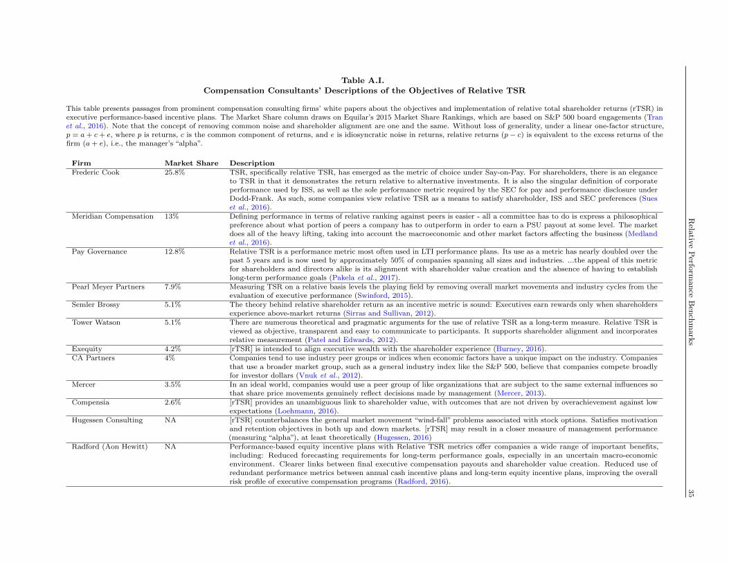
Rela

tive

Perfo

rmance

Ben

chm

ark

s35

Table A.I.Compensation Consultants’ Descriptions of the Objectives of Relative TSR

This table presents passages from prominent compensation consulting firms’ white papers about the objectives and implementation of relative total shareholder returns (rTSR) inexecutive performance-based incentive plans. The Market Share column draws on Equilar’s 2015 Market Share Rankings, which are based on S&P 500 board engagements (Tranet al., 2016). Note that the concept of removing common noise and shareholder alignment are one and the same. Without loss of generality, under a linear one-factor structure,p = a+ c+ e, where p is returns, c is the common component of returns, and e is idiosyncratic noise in returns, relative returns (p− c) is equivalent to the excess returns of thefirm (a+ e), i.e., the manager’s “alpha”.

Firm Market Share DescriptionFrederic Cook 25.8% TSR, specifically relative TSR, has emerged as the metric of choice under Say-on-Pay. For shareholders, there is an elegance

to TSR in that it demonstrates the return relative to alternative investments. It is also the singular definition of corporateperformance used by ISS, as well as the sole performance metric required by the SEC for pay and performance disclosure underDodd-Frank. As such, some companies view relative TSR as a means to satisfy shareholder, ISS and SEC preferences (Sueset al., 2016).

Meridian Compensation 13% Defining performance in terms of relative ranking against peers is easier - all a committee has to do is express a philosophicalpreference about what portion of peers a company has to outperform in order to earn a PSU payout at some level. The marketdoes all of the heavy lifting, taking into account the macroeconomic and other market factors affecting the business (Medlandet al., 2016).

Pay Governance 12.8% Relative TSR is a performance metric most often used in LTI performance plans. Its use as a metric has nearly doubled over thepast 5 years and is now used by approximately 50% of companies spanning all sizes and industries. ...the appeal of this metricfor shareholders and directors alike is its alignment with shareholder value creation and the absence of having to establishlong-term performance goals (Pakela et al., 2017).

Pearl Meyer Partners 7.9% Measuring TSR on a relative basis levels the playing field by removing overall market movements and industry cycles from theevaluation of executive performance (Swinford, 2015).

Semler Brossy 5.1% The theory behind relative shareholder return as an incentive metric is sound: Executives earn rewards only when shareholdersexperience above-market returns (Sirras and Sullivan, 2012).

Tower Watson 5.1% There are numerous theoretical and pragmatic arguments for the use of relative TSR as a long-term measure. Relative TSR isviewed as objective, transparent and easy to communicate to participants. It supports shareholder alignment and incorporatesrelative measurement (Patel and Edwards, 2012).

Exequity 4.2% [rTSR] is intended to align executive wealth with the shareholder experience (Burney, 2016).CA Partners 4% Companies tend to use industry peer groups or indices when economic factors have a unique impact on the industry. Companies

that use a broader market group, such as a general industry index like the S&P 500, believe that companies compete broadlyfor investor dollars (Vnuk et al., 2012).

Mercer 3.5% In an ideal world, companies would use a peer group of like organizations that are subject to the same external influences sothat share price movements genuinely reflect decisions made by management (Mercer, 2013).

Compensia 2.6% [rTSR] provides an unambiguous link to shareholder value, with outcomes that are not driven by overachievement against lowexpectations (Loehmann, 2016).

Hugessen Consulting NA [rTSR] counterbalances the general market movement “wind-fall” problems associated with stock options. Satisfies motivationand retention objectives in both up and down markets. [rTSR] may result in a closer measure of management performance(measuring “alpha”), at least theoretically (Hugessen, 2016)

Radford (Aon Hewitt) NA Performance-based equity incentive plans with Relative TSR metrics offer companies a wide range of important benefits,including: Reduced forecasting requirements for long-term performance goals, especially in an uncertain macro-economicenvironment. Clearer links between final executive compensation payouts and shareholder value creation. Reduced use ofredundant performance metrics between annual cash incentive plans and long-term equity incentive plans, improving the overallrisk profile of executive compensation programs (Radford, 2016).

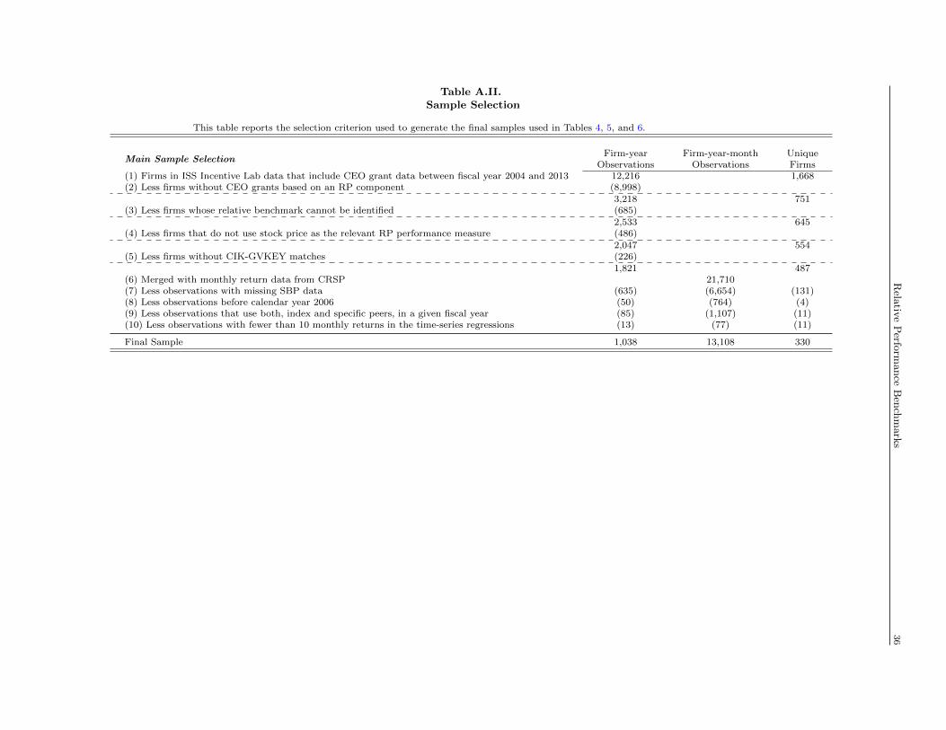
Rela

tive

Perfo

rmance

Ben

chm

ark

s36

Table A.II.Sample Selection

This table reports the selection criterion used to generate the final samples used in Tables 4, 5, and 6.

Main Sample SelectionFirm-year

ObservationsFirm-year-month

ObservationsUniqueFirms

(1) Firms in ISS Incentive Lab data that include CEO grant data between fiscal year 2004 and 2013 12,216 1,668(2) Less firms without CEO grants based on an RP component (8,998)

3,218 751(3) Less firms whose relative benchmark cannot be identified (685)

2,533 645(4) Less firms that do not use stock price as the relevant RP performance measure (486)

2,047 554(5) Less firms without CIK-GVKEY matches (226)

1,821 487(6) Merged with monthly return data from CRSP 21,710(7) Less observations with missing SBP data (635) (6,654) (131)(8) Less observations before calendar year 2006 (50) (764) (4)(9) Less observations that use both, index and specific peers, in a given fiscal year (85) (1,107) (11)(10) Less observations with fewer than 10 monthly returns in the time-series regressions (13) (77) (11)

Final Sample 1,038 13,108 330

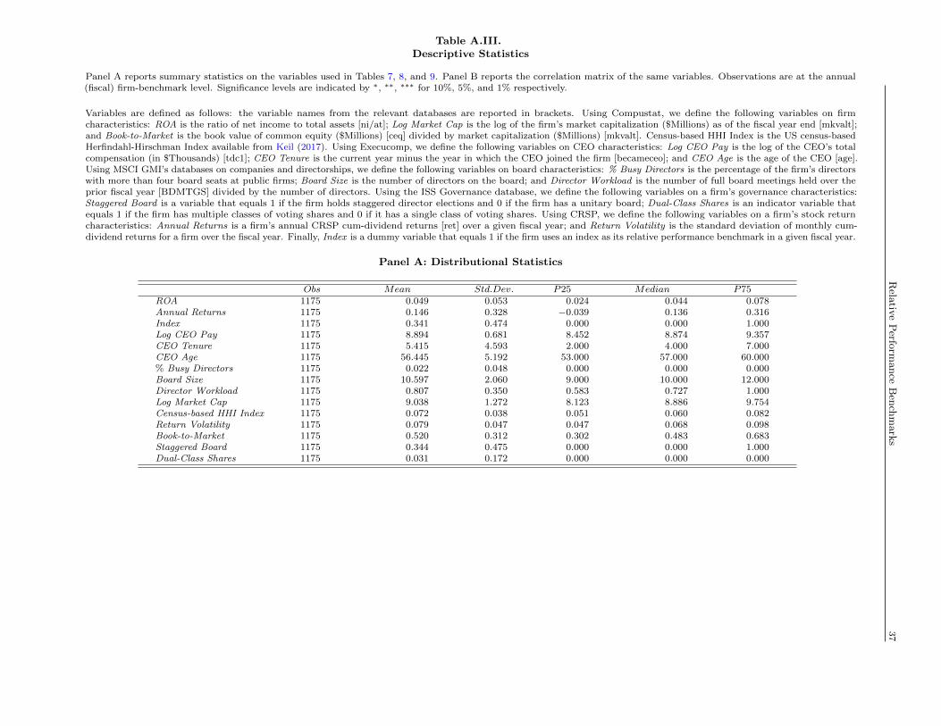
Rela

tive

Perfo

rmance

Ben

chm

ark

s37

Table A.III.Descriptive Statistics

Panel A reports summary statistics on the variables used in Tables 7, 8, and 9. Panel B reports the correlation matrix of the same variables. Observations are at the annual(fiscal) firm-benchmark level. Significance levels are indicated by ∗, ∗∗, ∗∗∗ for 10%, 5%, and 1% respectively.

Variables are defined as follows: the variable names from the relevant databases are reported in brackets. Using Compustat, we define the following variables on firmcharacteristics: ROA is the ratio of net income to total assets [ni/at]; Log Market Cap is the log of the firm’s market capitalization ($Millions) as of the fiscal year end [mkvalt];and Book-to-Market is the book value of common equity ($Millions) [ceq] divided by market capitalization ($Millions) [mkvalt]. Census-based HHI Index is the US census-basedHerfindahl-Hirschman Index available from Keil (2017). Using Execucomp, we define the following variables on CEO characteristics: Log CEO Pay is the log of the CEO’s totalcompensation (in $Thousands) [tdc1]; CEO Tenure is the current year minus the year in which the CEO joined the firm [becameceo]; and CEO Age is the age of the CEO [age].Using MSCI GMI’s databases on companies and directorships, we define the following variables on board characteristics: % Busy Directors is the percentage of the firm’s directorswith more than four board seats at public firms; Board Size is the number of directors on the board; and Director Workload is the number of full board meetings held over theprior fiscal year [BDMTGS] divided by the number of directors. Using the ISS Governance database, we define the following variables on a firm’s governance characteristics:Staggered Board is a variable that equals 1 if the firm holds staggered director elections and 0 if the firm has a unitary board; Dual-Class Shares is an indicator variable thatequals 1 if the firm has multiple classes of voting shares and 0 if it has a single class of voting shares. Using CRSP, we define the following variables on a firm’s stock returncharacteristics: Annual Returns is a firm’s annual CRSP cum-dividend returns [ret] over a given fiscal year; and Return Volatility is the standard deviation of monthly cum-dividend returns for a firm over the fiscal year. Finally, Index is a dummy variable that equals 1 if the firm uses an index as its relative performance benchmark in a given fiscal year.

Panel A: Distributional Statistics

Obs Mean Std.Dev. P25 Median P75ROA 1175 0.049 0.053 0.024 0.044 0.078Annual Returns 1175 0.146 0.328 −0.039 0.136 0.316Index 1175 0.341 0.474 0.000 0.000 1.000Log CEO Pay 1175 8.894 0.681 8.452 8.874 9.357CEO Tenure 1175 5.415 4.593 2.000 4.000 7.000CEO Age 1175 56.445 5.192 53.000 57.000 60.000% Busy Directors 1175 0.022 0.048 0.000 0.000 0.000Board Size 1175 10.597 2.060 9.000 10.000 12.000Director Workload 1175 0.807 0.350 0.583 0.727 1.000Log Market Cap 1175 9.038 1.272 8.123 8.886 9.754Census-based HHI Index 1175 0.072 0.038 0.051 0.060 0.082Return Volatility 1175 0.079 0.047 0.047 0.068 0.098Book-to-Market 1175 0.520 0.312 0.302 0.483 0.683Staggered Board 1175 0.344 0.475 0.000 0.000 1.000Dual-Class Shares 1175 0.031 0.172 0.000 0.000 0.000

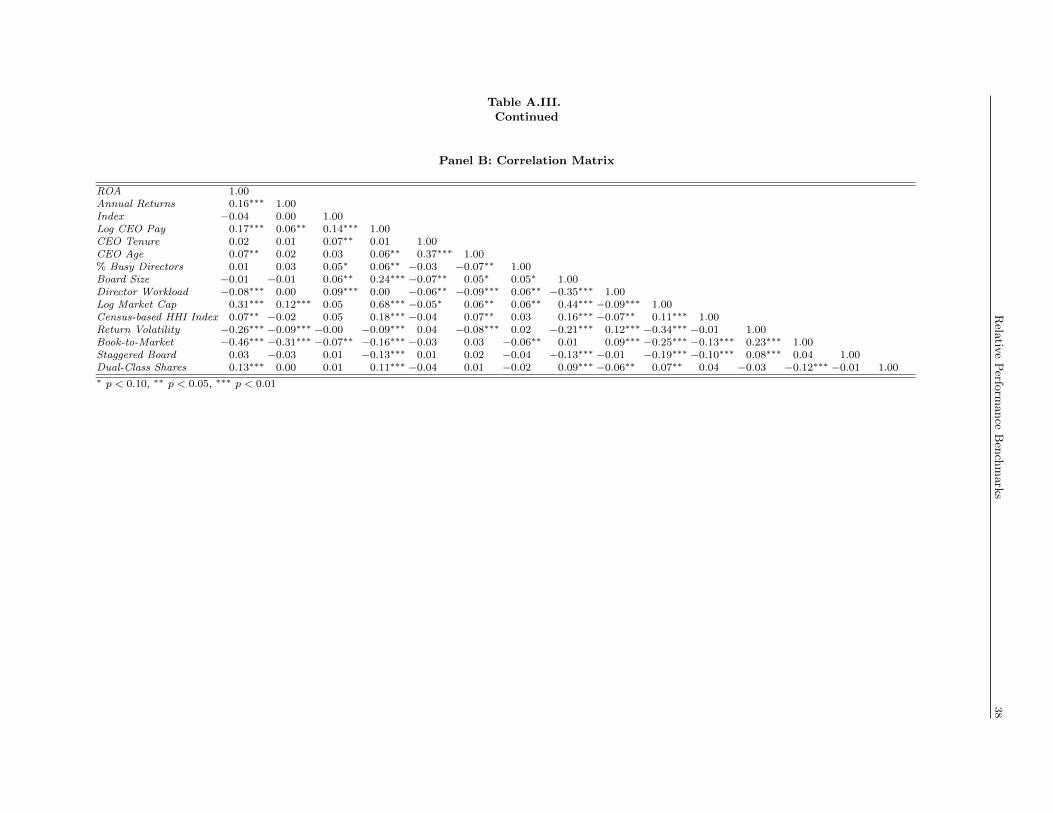
Rela

tive

Perfo

rmance

Ben

chm

ark

s38

Table A.III.Continued

Panel B: Correlation Matrix

ROA 1.00Annual Returns 0.16∗∗∗ 1.00Index −0.04 0.00 1.00Log CEO Pay 0.17∗∗∗ 0.06∗∗ 0.14∗∗∗ 1.00CEO Tenure 0.02 0.01 0.07∗∗ 0.01 1.00CEO Age 0.07∗∗ 0.02 0.03 0.06∗∗ 0.37∗∗∗ 1.00% Busy Directors 0.01 0.03 0.05∗ 0.06∗∗ −0.03 −0.07∗∗ 1.00Board Size −0.01 −0.01 0.06∗∗ 0.24∗∗∗ −0.07∗∗ 0.05∗ 0.05∗ 1.00Director Workload −0.08∗∗∗ 0.00 0.09∗∗∗ 0.00 −0.06∗∗ −0.09∗∗∗ 0.06∗∗ −0.35∗∗∗ 1.00Log Market Cap 0.31∗∗∗ 0.12∗∗∗ 0.05 0.68∗∗∗ −0.05∗ 0.06∗∗ 0.06∗∗ 0.44∗∗∗ −0.09∗∗∗ 1.00Census-based HHI Index 0.07∗∗ −0.02 0.05 0.18∗∗∗ −0.04 0.07∗∗ 0.03 0.16∗∗∗ −0.07∗∗ 0.11∗∗∗ 1.00Return Volatility −0.26∗∗∗ −0.09∗∗∗ −0.00 −0.09∗∗∗ 0.04 −0.08∗∗∗ 0.02 −0.21∗∗∗ 0.12∗∗∗ −0.34∗∗∗ −0.01 1.00Book-to-Market −0.46∗∗∗ −0.31∗∗∗ −0.07∗∗ −0.16∗∗∗ −0.03 0.03 −0.06∗∗ 0.01 0.09∗∗∗ −0.25∗∗∗ −0.13∗∗∗ 0.23∗∗∗ 1.00Staggered Board 0.03 −0.03 0.01 −0.13∗∗∗ 0.01 0.02 −0.04 −0.13∗∗∗ −0.01 −0.19∗∗∗ −0.10∗∗∗ 0.08∗∗∗ 0.04 1.00Dual-Class Shares 0.13∗∗∗ 0.00 0.01 0.11∗∗∗ −0.04 0.01 −0.02 0.09∗∗∗ −0.06∗∗ 0.07∗∗ 0.04 −0.03 −0.12∗∗∗ −0.01 1.00∗ p < 0.10, ∗∗ p < 0.05, ∗∗∗ p < 0.01

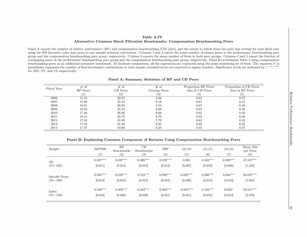
Rela

tive

Perfo

rmance

Ben

chm

ark

s39

Table A.IV.Alternative Common Shock Filtration Benchmarks: Compensation Benchmarking Peers

Panel A reports the number of relative performance (RP) and compensation benchmarking (CB) peers, and the extent to which these two peer sets overlap for each fiscal yearusing the ISS Incentive Labs data prior to any sample selection restrictions. Columns 1 and 2 report the mean number of chosen peers in the performance benchmarking peergroup and the compensation benchmarking peer group, respectively. Column 3 reports the mean number of firms in both peer groups. Columns 4 and 5 report the fraction ofoverlapping peers in the performance benchmarking peer group and the compensation benchmarking peer group, respectively. Panel B re-estimates Table 4 using compensationbenchmarking peers as an additional normative benchmark. To facilitate comparisons, all the regressions are conducted using the same underlying set of firms. The reported N inparentheses represents the number of firm-benchmark combinations in each sample; standard errors are reported in square brackets. Significance levels are indicated by ∗, ∗∗, ∗∗∗

for 10%, 5%, and 1% respectively.

Panel A: Summary Statistics of RP and CB Peers

Fiscal Year# of

RP Peers# of

CB Peers# of

Overlap PeersProportion RP Peers

Also in CB PeersProportion of CB Peers

Also in RP Peers(1) (2) (3) (4) (5)

2006 15.18 20.55 8.66 0.63 0.472007 15.90 25.44 9.18 0.67 0.472008 16.81 26.93 8.54 0.67 0.492009 16.56 25.55 8.68 0.63 0.462010 17.30 26.06 8.66 0.62 0.462011 18.21 25.79 8.70 0.62 0.462012 17.24 21.09 7.78 0.62 0.432013 17.84 21.83 6.83 0.60 0.402014 17.37 19.60 6.25 0.55 0.37

Panel B: Explaining Common Component of Returns Using Compensation Benchmarking Peers

Sample S&P500RP

BenchmarksCB

BenchmarksSBP (2)-(3) (3)-(1) (4)-(3)

Mean Obsper Firm

(1) (2) (3) (4) (5) (6) (7) (8)

All0.337∗∗∗ 0.497∗∗∗ 0.496∗∗∗ 0.525∗∗∗ 0.001 0.160∗∗∗ 0.029∗∗∗ 37.547∗∗∗

(N= 322) [0.011] [0.013] [0.012] [0.013] [0.007] [0.010] [0.008] [1.433]

Specific Peers0.335∗∗∗ 0.559∗∗∗ 0.534∗∗∗ 0.568∗∗∗ 0.025∗∗∗ 0.200∗∗∗ 0.034∗∗∗ 40.837∗∗∗

(N= 190) [0.013] [0.015] [0.015] [0.015] [0.008] [0.014] [0.010] [1.921]

Index0.340∗∗∗ 0.409∗∗∗ 0.442∗∗∗ 0.464∗∗∗ -0.033∗∗∗ 0.102∗∗∗ 0.023∗ 32.811∗∗∗

(N= 132) [0.018] [0.020] [0.020] [0.021] [0.011] [0.015] [0.013] [2.079]

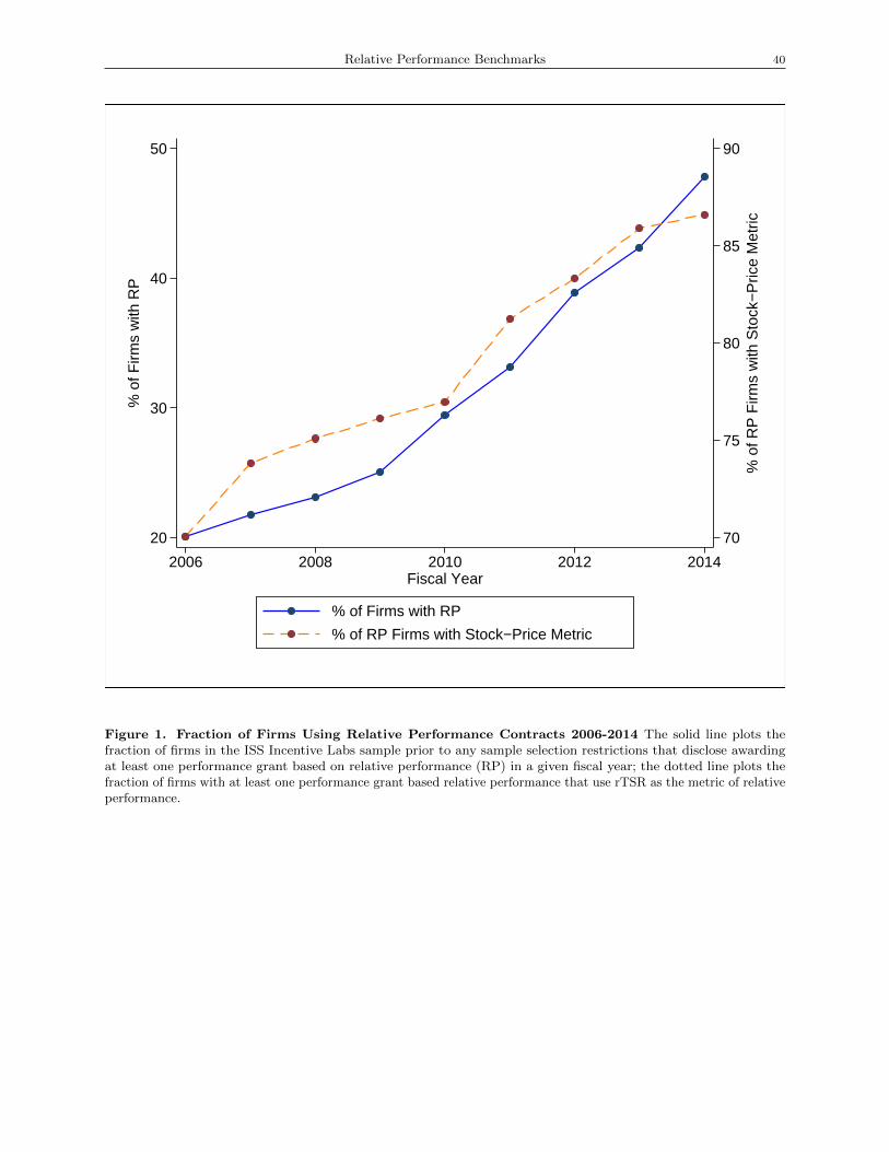
Relative Performance Benchmarks 40

70

75

80

85

90

% o

f RP

Firm

s w

ith S

tock

−P

rice

Met

ric

20

30

40

50%

of F

irms

with

RP

2006 2008 2010 2012 2014Fiscal Year

% of Firms with RP

% of RP Firms with Stock−Price Metric

Figure 1. Fraction of Firms Using Relative Performance Contracts 2006-2014 The solid line plots thefraction of firms in the ISS Incentive Labs sample prior to any sample selection restrictions that disclose awardingat least one performance grant based on relative performance (RP) in a given fiscal year; the dotted line plots thefraction of firms with at least one performance grant based relative performance that use rTSR as the metric of relativeperformance.

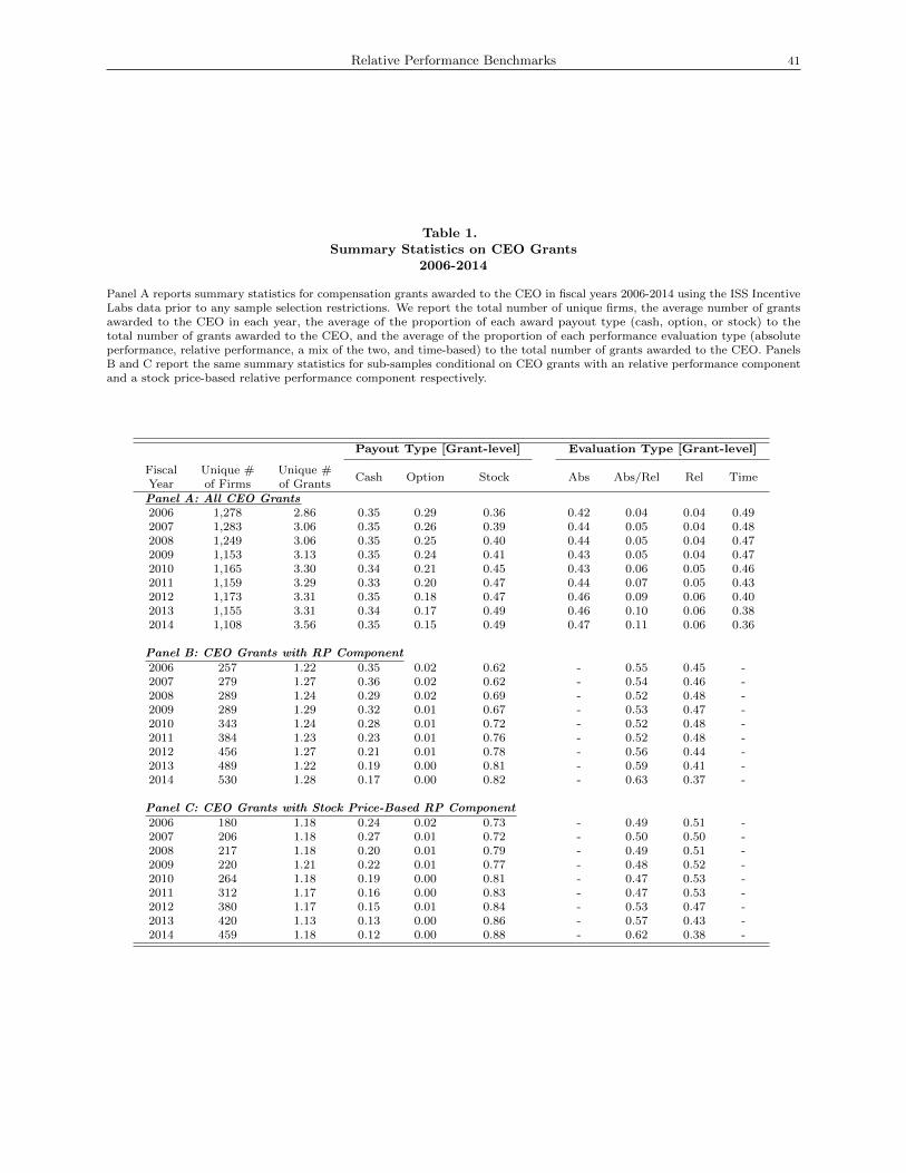
Relative Performance Benchmarks 41

Table 1.Summary Statistics on CEO Grants

2006-2014

Panel A reports summary statistics for compensation grants awarded to the CEO in fiscal years 2006-2014 using the ISS IncentiveLabs data prior to any sample selection restrictions. We report the total number of unique firms, the average number of grantsawarded to the CEO in each year, the average of the proportion of each award payout type (cash, option, or stock) to thetotal number of grants awarded to the CEO, and the average of the proportion of each performance evaluation type (absoluteperformance, relative performance, a mix of the two, and time-based) to the total number of grants awarded to the CEO. PanelsB and C report the same summary statistics for sub-samples conditional on CEO grants with an relative performance componentand a stock price-based relative performance component respectively.

Payout Type [Grant-level] Evaluation Type [Grant-level]

FiscalYear

Unique #of Firms

Unique #of Grants

Cash Option Stock Abs Abs/Rel Rel Time

Panel A: All CEO Grants2006 1,278 2.86 0.35 0.29 0.36 0.42 0.04 0.04 0.492007 1,283 3.06 0.35 0.26 0.39 0.44 0.05 0.04 0.482008 1,249 3.06 0.35 0.25 0.40 0.44 0.05 0.04 0.472009 1,153 3.13 0.35 0.24 0.41 0.43 0.05 0.04 0.472010 1,165 3.30 0.34 0.21 0.45 0.43 0.06 0.05 0.462011 1,159 3.29 0.33 0.20 0.47 0.44 0.07 0.05 0.432012 1,173 3.31 0.35 0.18 0.47 0.46 0.09 0.06 0.402013 1,155 3.31 0.34 0.17 0.49 0.46 0.10 0.06 0.382014 1,108 3.56 0.35 0.15 0.49 0.47 0.11 0.06 0.36

Panel B: CEO Grants with RP Component2006 257 1.22 0.35 0.02 0.62 - 0.55 0.45 -2007 279 1.27 0.36 0.02 0.62 - 0.54 0.46 -2008 289 1.24 0.29 0.02 0.69 - 0.52 0.48 -2009 289 1.29 0.32 0.01 0.67 - 0.53 0.47 -2010 343 1.24 0.28 0.01 0.72 - 0.52 0.48 -2011 384 1.23 0.23 0.01 0.76 - 0.52 0.48 -2012 456 1.27 0.21 0.01 0.78 - 0.56 0.44 -2013 489 1.22 0.19 0.00 0.81 - 0.59 0.41 -2014 530 1.28 0.17 0.00 0.82 - 0.63 0.37 -

Panel C: CEO Grants with Stock Price-Based RP Component2006 180 1.18 0.24 0.02 0.73 - 0.49 0.51 -2007 206 1.18 0.27 0.01 0.72 - 0.50 0.50 -2008 217 1.18 0.20 0.01 0.79 - 0.49 0.51 -2009 220 1.21 0.22 0.01 0.77 - 0.48 0.52 -2010 264 1.18 0.19 0.00 0.81 - 0.47 0.53 -2011 312 1.17 0.16 0.00 0.83 - 0.47 0.53 -2012 380 1.17 0.15 0.01 0.84 - 0.53 0.47 -2013 420 1.13 0.13 0.00 0.86 - 0.57 0.43 -2014 459 1.18 0.12 0.00 0.88 - 0.62 0.38 -

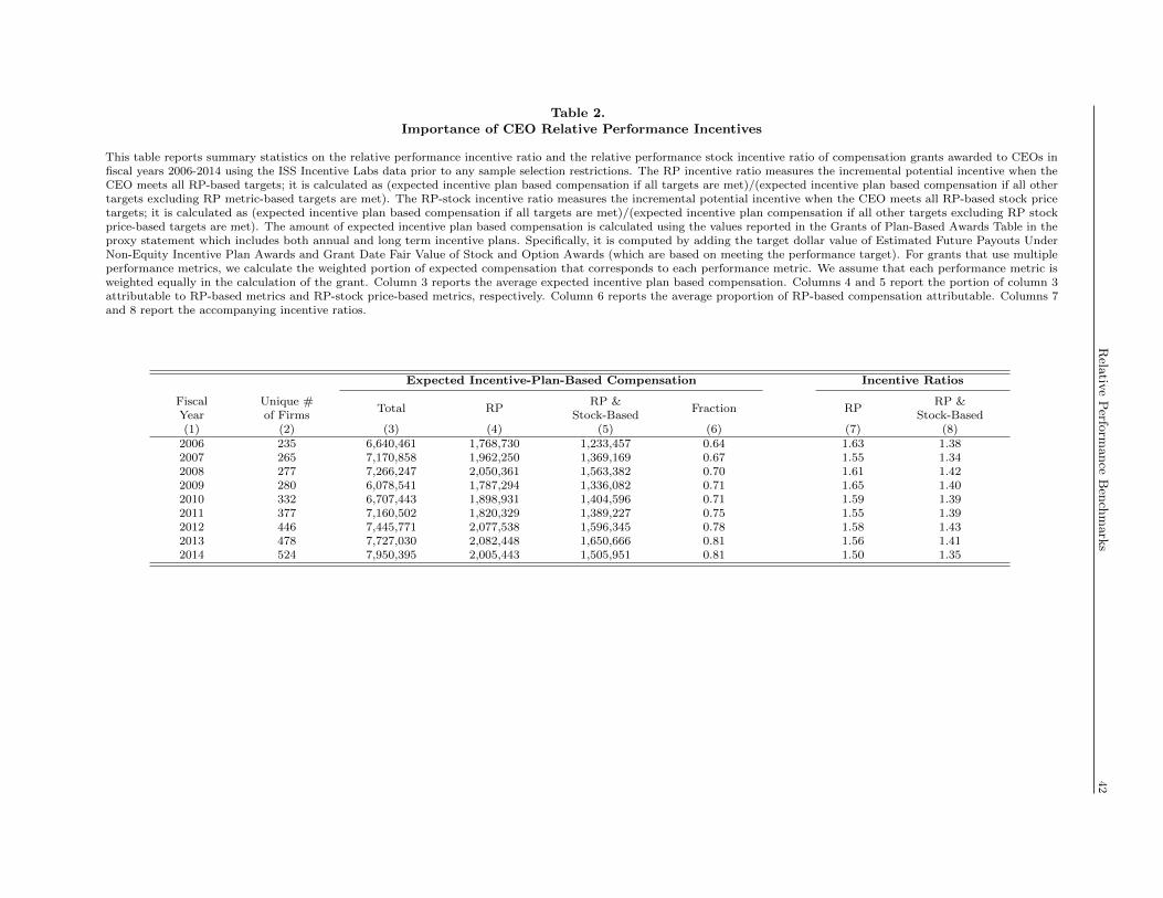
Rela

tive

Perfo

rmance

Ben

chm

ark

s42

Table 2.Importance of CEO Relative Performance Incentives

This table reports summary statistics on the relative performance incentive ratio and the relative performance stock incentive ratio of compensation grants awarded to CEOs infiscal years 2006-2014 using the ISS Incentive Labs data prior to any sample selection restrictions. The RP incentive ratio measures the incremental potential incentive when theCEO meets all RP-based targets; it is calculated as (expected incentive plan based compensation if all targets are met)/(expected incentive plan based compensation if all othertargets excluding RP metric-based targets are met). The RP-stock incentive ratio measures the incremental potential incentive when the CEO meets all RP-based stock pricetargets; it is calculated as (expected incentive plan based compensation if all targets are met)/(expected incentive plan compensation if all other targets excluding RP stockprice-based targets are met). The amount of expected incentive plan based compensation is calculated using the values reported in the Grants of Plan-Based Awards Table in theproxy statement which includes both annual and long term incentive plans. Specifically, it is computed by adding the target dollar value of Estimated Future Payouts UnderNon-Equity Incentive Plan Awards and Grant Date Fair Value of Stock and Option Awards (which are based on meeting the performance target). For grants that use multipleperformance metrics, we calculate the weighted portion of expected compensation that corresponds to each performance metric. We assume that each performance metric isweighted equally in the calculation of the grant. Column 3 reports the average expected incentive plan based compensation. Columns 4 and 5 report the portion of column 3attributable to RP-based metrics and RP-stock price-based metrics, respectively. Column 6 reports the average proportion of RP-based compensation attributable. Columns 7and 8 report the accompanying incentive ratios.

Expected Incentive-Plan-Based Compensation Incentive Ratios

FiscalYear

Unique #of Firms

Total RPRP &

Stock-BasedFraction RP

RP &Stock-Based

(1) (2) (3) (4) (5) (6) (7) (8)2006 235 6,640,461 1,768,730 1,233,457 0.64 1.63 1.382007 265 7,170,858 1,962,250 1,369,169 0.67 1.55 1.342008 277 7,266,247 2,050,361 1,563,382 0.70 1.61 1.422009 280 6,078,541 1,787,294 1,336,082 0.71 1.65 1.402010 332 6,707,443 1,898,931 1,404,596 0.71 1.59 1.392011 377 7,160,502 1,820,329 1,389,227 0.75 1.55 1.392012 446 7,445,771 2,077,538 1,596,345 0.78 1.58 1.432013 478 7,727,030 2,082,448 1,650,666 0.81 1.56 1.412014 524 7,950,395 2,005,443 1,505,951 0.81 1.50 1.35

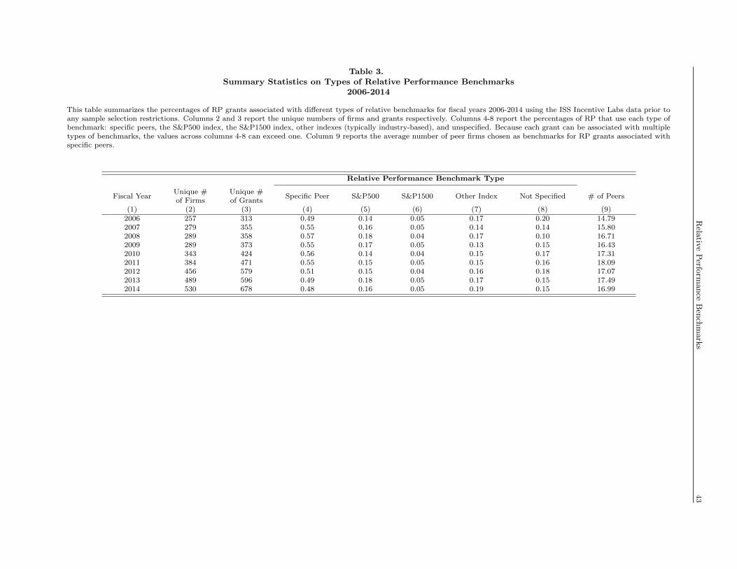
Rela

tive

Perfo

rmance

Ben

chm

ark

s43

Table 3.Summary Statistics on Types of Relative Performance Benchmarks

2006-2014

This table summarizes the percentages of RP grants associated with different types of relative benchmarks for fiscal years 2006-2014 using the ISS Incentive Labs data prior toany sample selection restrictions. Columns 2 and 3 report the unique numbers of firms and grants respectively. Columns 4-8 report the percentages of RP that use each type ofbenchmark: specific peers, the S&P500 index, the S&P1500 index, other indexes (typically industry-based), and unspecified. Because each grant can be associated with multipletypes of benchmarks, the values across columns 4-8 can exceed one. Column 9 reports the average number of peer firms chosen as benchmarks for RP grants associated withspecific peers.

Relative Performance Benchmark Type

Fiscal YearUnique #of Firms

Unique #of Grants

Specific Peer S&P500 S&P1500 Other Index Not Specified # of Peers

(1) (2) (3) (4) (5) (6) (7) (8) (9)2006 257 313 0.49 0.14 0.05 0.17 0.20 14.792007 279 355 0.55 0.16 0.05 0.14 0.14 15.802008 289 358 0.57 0.18 0.04 0.17 0.10 16.712009 289 373 0.55 0.17 0.05 0.13 0.15 16.432010 343 424 0.56 0.14 0.04 0.15 0.17 17.312011 384 471 0.55 0.15 0.05 0.15 0.16 18.092012 456 579 0.51 0.15 0.04 0.16 0.18 17.072013 489 596 0.49 0.18 0.05 0.17 0.15 17.492014 530 678 0.48 0.16 0.05 0.19 0.15 16.99

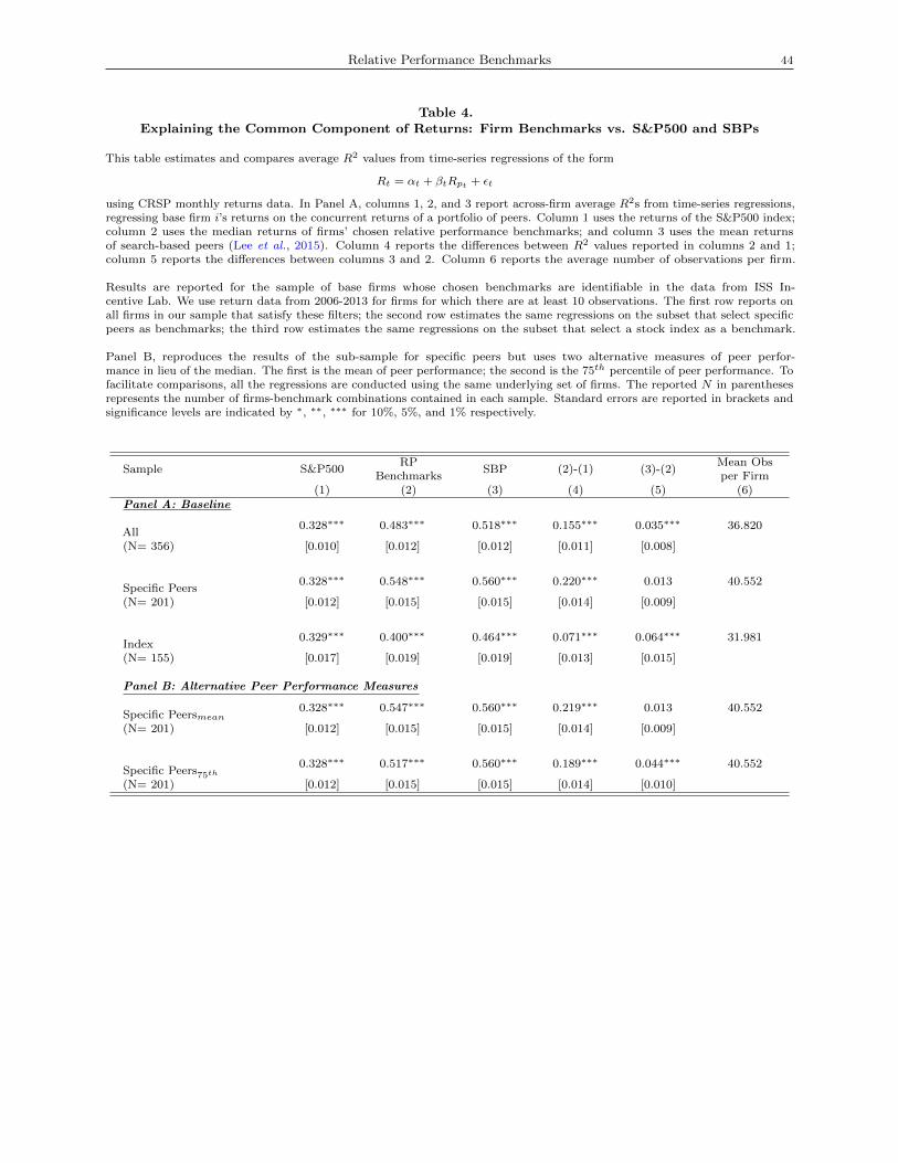
Relative Performance Benchmarks 44

Table 4.Explaining the Common Component of Returns: Firm Benchmarks vs. S&P500 and SBPs

This table estimates and compares average R2 values from time-series regressions of the form

Rt = αt + βtRpt + εt

using CRSP monthly returns data. In Panel A, columns 1, 2, and 3 report across-firm average R2s from time-series regressions,regressing base firm i’s returns on the concurrent returns of a portfolio of peers. Column 1 uses the returns of the S&P500 index;column 2 uses the median returns of firms’ chosen relative performance benchmarks; and column 3 uses the mean returnsof search-based peers (Lee et al., 2015). Column 4 reports the differences between R2 values reported in columns 2 and 1;column 5 reports the differences between columns 3 and 2. Column 6 reports the average number of observations per firm.

Results are reported for the sample of base firms whose chosen benchmarks are identifiable in the data from ISS In-centive Lab. We use return data from 2006-2013 for firms for which there are at least 10 observations. The first row reports onall firms in our sample that satisfy these filters; the second row estimates the same regressions on the subset that select specificpeers as benchmarks; the third row estimates the same regressions on the subset that select a stock index as a benchmark.

Panel B, reproduces the results of the sub-sample for specific peers but uses two alternative measures of peer perfor-mance in lieu of the median. The first is the mean of peer performance; the second is the 75th percentile of peer performance. Tofacilitate comparisons, all the regressions are conducted using the same underlying set of firms. The reported N in parenthesesrepresents the number of firms-benchmark combinations contained in each sample. Standard errors are reported in brackets andsignificance levels are indicated by ∗, ∗∗, ∗∗∗ for 10%, 5%, and 1% respectively.

Sample S&P500RP

BenchmarksSBP (2)-(1) (3)-(2)

Mean Obsper Firm

(1) (2) (3) (4) (5) (6)Panel A: Baseline

All0.328∗∗∗ 0.483∗∗∗ 0.518∗∗∗ 0.155∗∗∗ 0.035∗∗∗ 36.820

(N= 356) [0.010] [0.012] [0.012] [0.011] [0.008]

Specific Peers0.328∗∗∗ 0.548∗∗∗ 0.560∗∗∗ 0.220∗∗∗ 0.013 40.552

(N= 201) [0.012] [0.015] [0.015] [0.014] [0.009]

Index0.329∗∗∗ 0.400∗∗∗ 0.464∗∗∗ 0.071∗∗∗ 0.064∗∗∗ 31.981

(N= 155) [0.017] [0.019] [0.019] [0.013] [0.015]

Panel B: Alternative Peer Performance Measures

Specific Peersmean0.328∗∗∗ 0.547∗∗∗ 0.560∗∗∗ 0.219∗∗∗ 0.013 40.552

(N= 201) [0.012] [0.015] [0.015] [0.014] [0.009]

Specific Peers75th0.328∗∗∗ 0.517∗∗∗ 0.560∗∗∗ 0.189∗∗∗ 0.044∗∗∗ 40.552

(N= 201) [0.012] [0.015] [0.015] [0.014] [0.010]

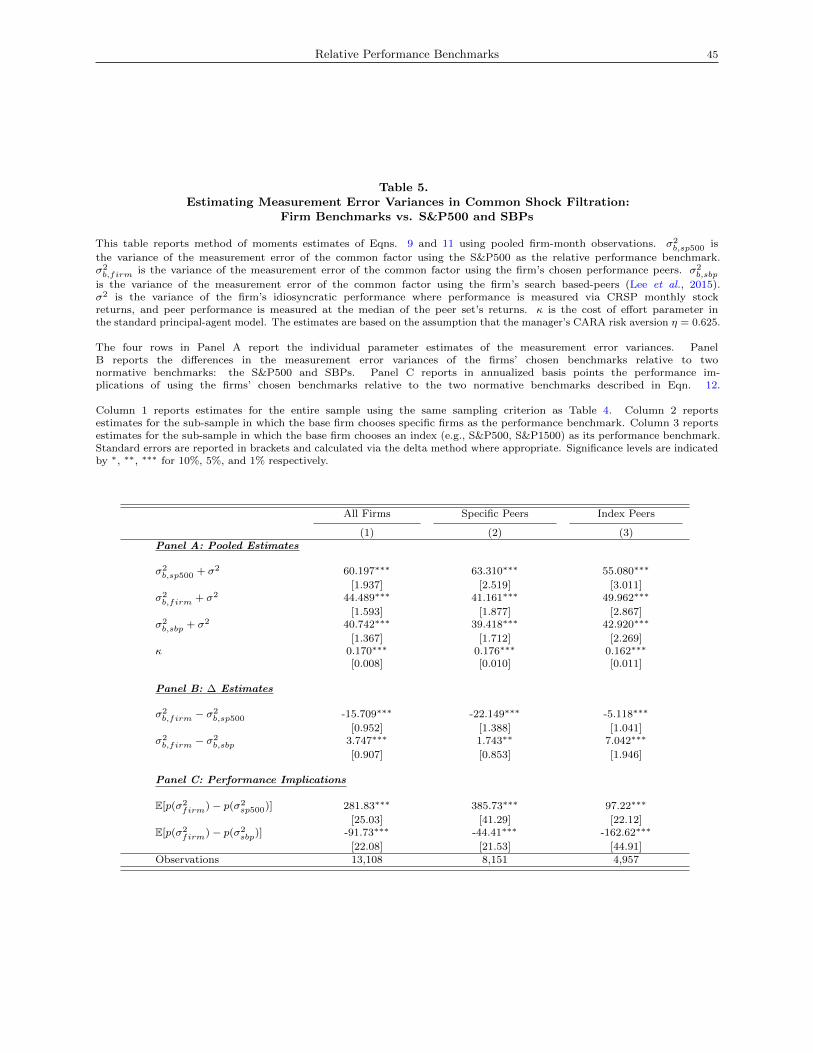
Relative Performance Benchmarks 45

Table 5.Estimating Measurement Error Variances in Common Shock Filtration:

Firm Benchmarks vs. S&P500 and SBPs

This table reports method of moments estimates of Eqns. 9 and 11 using pooled firm-month observations. σ2b,sp500 is

the variance of the measurement error of the common factor using the S&P500 as the relative performance benchmark.σ2b,firm is the variance of the measurement error of the common factor using the firm’s chosen performance peers. σ2

b,sbp

is the variance of the measurement error of the common factor using the firm’s search based-peers (Lee et al., 2015).σ2 is the variance of the firm’s idiosyncratic performance where performance is measured via CRSP monthly stockreturns, and peer performance is measured at the median of the peer set’s returns. κ is the cost of effort parameter inthe standard principal-agent model. The estimates are based on the assumption that the manager’s CARA risk aversion η = 0.625.

The four rows in Panel A report the individual parameter estimates of the measurement error variances. PanelB reports the differences in the measurement error variances of the firms’ chosen benchmarks relative to twonormative benchmarks: the S&P500 and SBPs. Panel C reports in annualized basis points the performance im-plications of using the firms’ chosen benchmarks relative to the two normative benchmarks described in Eqn. 12.

Column 1 reports estimates for the entire sample using the same sampling criterion as Table 4. Column 2 reportsestimates for the sub-sample in which the base firm chooses specific firms as the performance benchmark. Column 3 reportsestimates for the sub-sample in which the base firm chooses an index (e.g., S&P500, S&P1500) as its performance benchmark.Standard errors are reported in brackets and calculated via the delta method where appropriate. Significance levels are indicatedby ∗, ∗∗, ∗∗∗ for 10%, 5%, and 1% respectively.

All Firms Specific Peers Index Peers

(1) (2) (3)Panel A: Pooled Estimates

σ2b,sp500 + σ2 60.197∗∗∗ 63.310∗∗∗ 55.080∗∗∗

[1.937] [2.519] [3.011]σ2b,firm + σ2 44.489∗∗∗ 41.161∗∗∗ 49.962∗∗∗

[1.593] [1.877] [2.867]σ2b,sbp + σ2 40.742∗∗∗ 39.418∗∗∗ 42.920∗∗∗

[1.367] [1.712] [2.269]κ 0.170∗∗∗ 0.176∗∗∗ 0.162∗∗∗

[0.008] [0.010] [0.011]

Panel B: ∆ Estimates

σ2b,firm − σ

2b,sp500 -15.709∗∗∗ -22.149∗∗∗ -5.118∗∗∗

[0.952] [1.388] [1.041]σ2b,firm − σ

2b,sbp 3.747∗∗∗ 1.743∗∗ 7.042∗∗∗

[0.907] [0.853] [1.946]

Panel C: Performance Implications

E[p(σ2firm)− p(σ2

sp500)] 281.83∗∗∗ 385.73∗∗∗ 97.22∗∗∗

[25.03] [41.29] [22.12]E[p(σ2

firm)− p(σ2sbp)] -91.73∗∗∗ -44.41∗∗∗ -162.62∗∗∗

[22.08] [21.53] [44.91]Observations 13,108 8,151 4,957

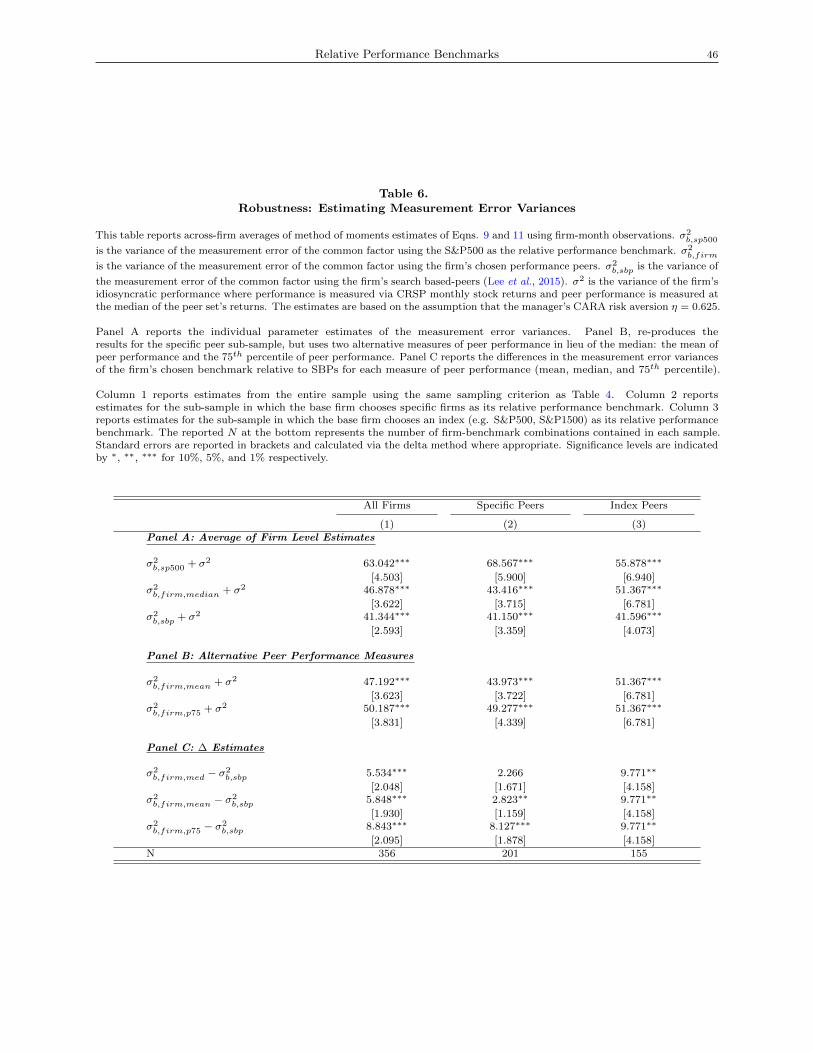
Relative Performance Benchmarks 46

Table 6.Robustness: Estimating Measurement Error Variances

This table reports across-firm averages of method of moments estimates of Eqns. 9 and 11 using firm-month observations. σ2b,sp500is the variance of the measurement error of the common factor using the S&P500 as the relative performance benchmark. σ2b,firmis the variance of the measurement error of the common factor using the firm’s chosen performance peers. σ2b,sbp is the variance of

the measurement error of the common factor using the firm’s search based-peers (Lee et al., 2015). σ2 is the variance of the firm’sidiosyncratic performance where performance is measured via CRSP monthly stock returns and peer performance is measured atthe median of the peer set’s returns. The estimates are based on the assumption that the manager’s CARA risk aversion η = 0.625.

Panel A reports the individual parameter estimates of the measurement error variances. Panel B, re-produces theresults for the specific peer sub-sample, but uses two alternative measures of peer performance in lieu of the median: the mean ofpeer performance and the 75th percentile of peer performance. Panel C reports the differences in the measurement error variancesof the firm’s chosen benchmark relative to SBPs for each measure of peer performance (mean, median, and 75th percentile).

Column 1 reports estimates from the entire sample using the same sampling criterion as Table 4. Column 2 reportsestimates for the sub-sample in which the base firm chooses specific firms as its relative performance benchmark. Column 3reports estimates for the sub-sample in which the base firm chooses an index (e.g. S&P500, S&P1500) as its relative performancebenchmark. The reported N at the bottom represents the number of firm-benchmark combinations contained in each sample.Standard errors are reported in brackets and calculated via the delta method where appropriate. Significance levels are indicatedby ∗, ∗∗, ∗∗∗ for 10%, 5%, and 1% respectively.

All Firms Specific Peers Index Peers

(1) (2) (3)Panel A: Average of Firm Level Estimates

σ2b,sp500 + σ2 63.042∗∗∗ 68.567∗∗∗ 55.878∗∗∗

[4.503] [5.900] [6.940]σ2b,firm,median + σ2 46.878∗∗∗ 43.416∗∗∗ 51.367∗∗∗

[3.622] [3.715] [6.781]σ2b,sbp + σ2 41.344∗∗∗ 41.150∗∗∗ 41.596∗∗∗

[2.593] [3.359] [4.073]

Panel B: Alternative Peer Performance Measures

σ2b,firm,mean + σ2 47.192∗∗∗ 43.973∗∗∗ 51.367∗∗∗

[3.623] [3.722] [6.781]σ2b,firm,p75 + σ2 50.187∗∗∗ 49.277∗∗∗ 51.367∗∗∗

[3.831] [4.339] [6.781]

Panel C: ∆ Estimates

σ2b,firm,med − σ

2b,sbp 5.534∗∗∗ 2.266 9.771∗∗

[2.048] [1.671] [4.158]σ2b,firm,mean − σ

2b,sbp 5.848∗∗∗ 2.823∗∗ 9.771∗∗

[1.930] [1.159] [4.158]σ2b,firm,p75 − σ

2b,sbp 8.843∗∗∗ 8.127∗∗∗ 9.771∗∗

[2.095] [1.878] [4.158]N 356 201 155

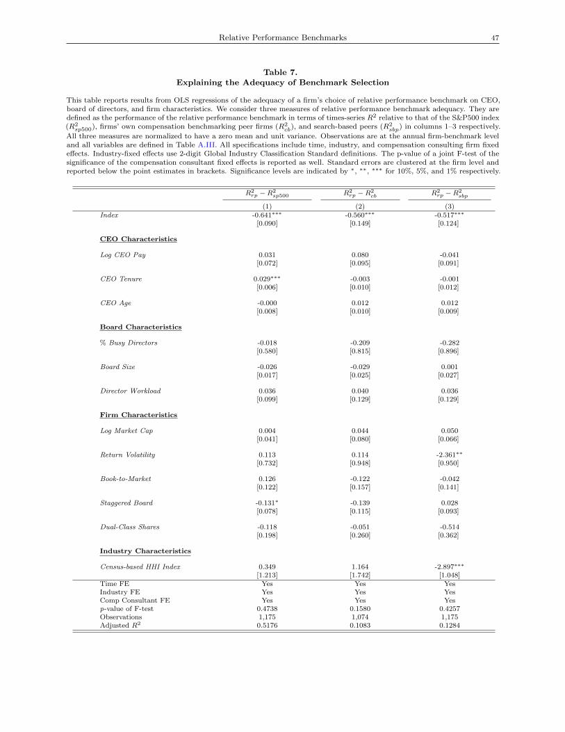
Relative Performance Benchmarks 47

Table 7.Explaining the Adequacy of Benchmark Selection

This table reports results from OLS regressions of the adequacy of a firm’s choice of relative performance benchmark on CEO,board of directors, and firm characteristics. We consider three measures of relative performance benchmark adequacy. They aredefined as the performance of the relative performance benchmark in terms of times-series R2 relative to that of the S&P500 index(R2sp500), firms’ own compensation benchmarking peer firms (R2

cb), and search-based peers (R2sbp) in columns 1–3 respectively.

All three measures are normalized to have a zero mean and unit variance. Observations are at the annual firm-benchmark leveland all variables are defined in Table A.III. All specifications include time, industry, and compensation consulting firm fixedeffects. Industry-fixed effects use 2-digit Global Industry Classification Standard definitions. The p-value of a joint F-test of thesignificance of the compensation consultant fixed effects is reported as well. Standard errors are clustered at the firm level andreported below the point estimates in brackets. Significance levels are indicated by ∗, ∗∗, ∗∗∗ for 10%, 5%, and 1% respectively.

R2rp −R2

sp500 R2rp −R2

cb R2rp −R2

sbp

(1) (2) (3)Index -0.641∗∗∗ -0.560∗∗∗ -0.517∗∗∗

[0.090] [0.149] [0.124]

CEO Characteristics

Log CEO Pay 0.031 0.080 -0.041[0.072] [0.095] [0.091]

CEO Tenure 0.029∗∗∗ -0.003 -0.001[0.006] [0.010] [0.012]

CEO Age -0.000 0.012 0.012[0.008] [0.010] [0.009]

Board Characteristics

% Busy Directors -0.018 -0.209 -0.282[0.580] [0.815] [0.896]

Board Size -0.026 -0.029 0.001[0.017] [0.025] [0.027]

Director Workload 0.036 0.040 0.036[0.099] [0.129] [0.129]

Firm Characteristics

Log Market Cap 0.004 0.044 0.050[0.041] [0.080] [0.066]

Return Volatility 0.113 0.114 -2.361∗∗

[0.732] [0.948] [0.950]

Book-to-Market 0.126 -0.122 -0.042[0.122] [0.157] [0.141]

Staggered Board -0.131∗ -0.139 0.028[0.078] [0.115] [0.093]

Dual-Class Shares -0.118 -0.051 -0.514[0.198] [0.260] [0.362]

Industry Characteristics

Census-based HHI Index 0.349 1.164 -2.897∗∗∗

[1.213] [1.742] [1.048]Time FE Yes Yes YesIndustry FE Yes Yes YesComp Consultant FE Yes Yes Yesp-value of F-test 0.4738 0.1580 0.4257Observations 1,175 1,074 1,175Adjusted R2 0.5176 0.1083 0.1284

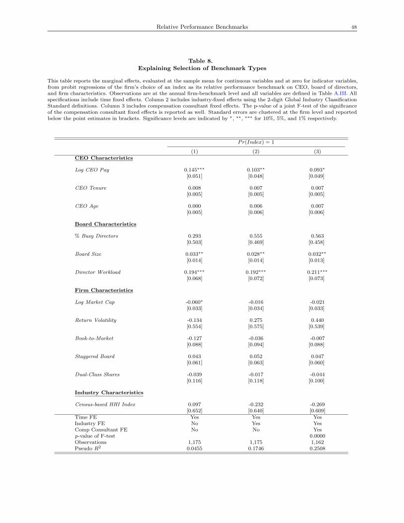
Relative Performance Benchmarks 48

Table 8.Explaining Selection of Benchmark Types

This table reports the marginal effects, evaluated at the sample mean for continuous variables and at zero for indicator variables,from probit regressions of the firm’s choice of an index as its relative performance benchmark on CEO, board of directors,and firm characteristics. Observations are at the annual firm-benchmark level and all variables are defined in Table A.III. Allspecifications include time fixed effects. Column 2 includes industry-fixed effects using the 2-digit Global Industry ClassificationStandard definitions. Column 3 includes compensation consultant fixed effects. The p-value of a joint F-test of the significanceof the compensation consultant fixed effects is reported as well. Standard errors are clustered at the firm level and reportedbelow the point estimates in brackets. Significance levels are indicated by ∗, ∗∗, ∗∗∗ for 10%, 5%, and 1% respectively.

Pr(Index) = 1

(1) (2) (3)CEO Characteristics

Log CEO Pay 0.145∗∗∗ 0.103∗∗ 0.093∗

[0.051] [0.048] [0.049]

CEO Tenure 0.008 0.007 0.007[0.005] [0.005] [0.005]

CEO Age 0.000 0.006 0.007[0.005] [0.006] [0.006]

Board Characteristics

% Busy Directors 0.293 0.555 0.563[0.503] [0.469] [0.458]

Board Size 0.033∗∗ 0.028∗∗ 0.032∗∗

[0.014] [0.014] [0.013]

Director Workload 0.194∗∗∗ 0.192∗∗∗ 0.211∗∗∗

[0.068] [0.072] [0.073]

Firm Characteristics

Log Market Cap -0.060∗ -0.016 -0.021[0.033] [0.034] [0.033]

Return Volatility -0.134 0.275 0.440[0.554] [0.575] [0.539]

Book-to-Market -0.127 -0.036 -0.007[0.088] [0.094] [0.088]

Staggered Board 0.043 0.052 0.047[0.061] [0.063] [0.060]

Dual-Class Shares -0.039 -0.017 -0.044[0.116] [0.118] [0.100]

Industry Characteristics

Census-based HHI Index 0.097 -0.232 -0.269[0.652] [0.640] [0.609]

Time FE Yes Yes YesIndustry FE No Yes YesComp Consultant FE No No Yesp-value of F-test 0.0000Observations 1,175 1,175 1,162Pseudo R2 0.0455 0.1746 0.2508

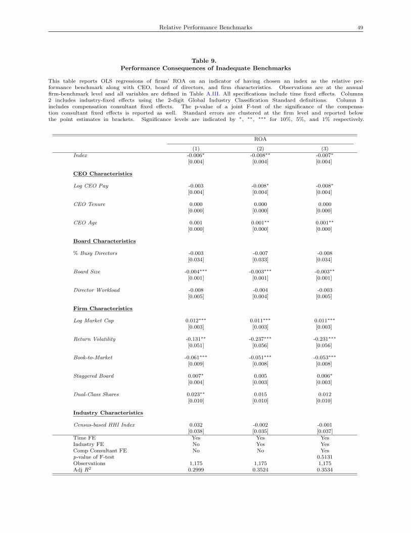
Relative Performance Benchmarks 49

Table 9.Performance Consequences of Inadequate Benchmarks

This table reports OLS regressions of firms’ ROA on an indicator of having chosen an index as the relative per-formance benchmark along with CEO, board of directors, and firm characteristics. Observations are at the annualfirm-benchmark level and all variables are defined in Table A.III. All specifications include time fixed effects. Columns2 includes industry-fixed effects using the 2-digit Global Industry Classification Standard definitions. Column 3includes compensation consultant fixed effects. The p-value of a joint F-test of the significance of the compensa-tion consultant fixed effects is reported as well. Standard errors are clustered at the firm level and reported belowthe point estimates in brackets. Significance levels are indicated by ∗, ∗∗, ∗∗∗ for 10%, 5%, and 1% respectively.

ROA

(1) (2) (3)Index -0.006∗ -0.008∗∗ -0.007∗

[0.004] [0.004] [0.004]

CEO Characteristics

Log CEO Pay -0.003 -0.008∗ -0.008∗

[0.004] [0.004] [0.004]

CEO Tenure 0.000 0.000 0.000[0.000] [0.000] [0.000]

CEO Age 0.001 0.001∗∗ 0.001∗∗

[0.000] [0.000] [0.000]

Board Characteristics

% Busy Directors -0.003 -0.007 -0.008[0.034] [0.033] [0.034]

Board Size -0.004∗∗∗ -0.003∗∗∗ -0.003∗∗

[0.001] [0.001] [0.001]

Director Workload -0.008 -0.004 -0.003[0.005] [0.004] [0.005]

Firm Characteristics

Log Market Cap 0.012∗∗∗ 0.011∗∗∗ 0.011∗∗∗

[0.003] [0.003] [0.003]

Return Volatility -0.131∗∗ -0.237∗∗∗ -0.231∗∗∗

[0.051] [0.056] [0.056]

Book-to-Market -0.061∗∗∗ -0.051∗∗∗ -0.053∗∗∗

[0.009] [0.008] [0.008]

Staggered Board 0.007∗ 0.005 0.006∗

[0.004] [0.003] [0.003]

Dual-Class Shares 0.023∗∗ 0.015 0.012[0.010] [0.010] [0.010]

Industry Characteristics

Census-based HHI Index 0.032 -0.002 -0.001[0.038] [0.035] [0.037]

Time FE Yes Yes YesIndustry FE No Yes YesComp Consultant FE No No Yesp-value of F-test 0.5131Observations 1,175 1,175 1,175Adj R2 0.2999 0.3524 0.3534