Relative Performance Banker Compensation

and Systemic Risk

Rui AlbuquerqueBoston College

Luıs CabralNew York University

Jose Correa GuedesCatolica Lisbon School of Business and Economics

October 2016

Abstract. This paper shows that in the presence of investment opportunities that arecorrelated, risk sharing between bank shareholders and bank managers leads to com-pensation contracts that include relative performance evaluation and to investmentdecisions that are biased to the more correlated opportunities, leading to systemicrisk. We analyse various policy recommendations regarding managerial pay at majorbanks and show that relative performance evaluation undoes most of the intendedrisk-reducing e↵ects of the policies, demonstrating their ine↵ectiveness in curbingsystemic risk.

Albuquerque: Associate Professor of Finance, Boston College Carroll School of Management;Research Associate, ECGI; and Research Fellow, CEPR; rui.albuquerque@bc.edu. Cabral:Paganelli-Bull Professor of Economics and International Business, Stern School of Business, NewYork University; and Research Fellow, CEPR; luis.cabral@nyu.edu. Guedes: Professor of Finance,Catolica Lisbon School of Business and Economics; jcg@ucp.pt

We thank Viral Acharya, Anat Admati, David Dicks, Nadya Malenko, and Kathy Yuan for usefulcomments and suggestions; the usual disclaimer applies. Albuquerque thanks the support fromfunding grant PTDC/IIM-FIN/2977/2014 of the Portuguese Foundation for Science andTechnology-FCT.

1. Introduction

Central banks around the world are entering unchartered territory by regulating payof bank Chief Executive O�cers (CEOs). These actions are a response to the viewthat bank executives’ compensation packages are one of the main culprits of the risktaking in the banking industry that preceded the recent financial crisis (e.g., Inter-national Monetary Fund, 2014). Loosely speaking, excessive risk can arise becausebank CEOs are shielded from significant negative shocks to their own banks becauseof poorly designed compensation packages (e.g., Admati and Hellwig, 2013; Interna-tional Monetary Fund, 2014; and Geithner, 2010). This paper provides a model witha novel mechanism through which pay of bank executives can lead to systemic risk inthe banking industry as it leads banks to take on correlated actions. It then uses themodel to analyze the e↵ectiveness of many of the new regulatory actions by centralbanks in reducing systemic risk.

The question we ask is whether optimally designed compensation packages, thatare not misaligned in any way by managerial entrenchment, can lead to systemic riskeven in the absence of bailout guarantees. The goal is to identify contractual featuresin compensation that can potentially lead to systemic risk and that thus warrant payregulation by a central bank who values social welfare losses from systemic risk.

We model two identical banks each bank with a risk-neutral principal (the share-holders) and a risk-averse agent (the CEO). Each bank has access to two investmentopportunities, one with only idiosyncratic risk and another that carries risk that iscorrelated across banks. The agent is required to spend costly unobservable e↵ort toincrease the return of the projects available to the bank and makes an unobservableportfolio allocation of how much of each investment opportunity to pursue. To focuson risk alone we assume equal expected returns to both projects and thus an equalcontribution of e↵ort to expected returns.

As in the classical principal-agent setting with hidden action, in our model theagent is induced to deploy unobservable e↵ort by linking her pay to the bank’s perfor-mance. However, because the agent is risk-averse, this contract can be improved byreducing the volatility in the compensation of the manager by incorporating relativeperformance evaluation (RPE). Having compensation depend on relative performancerather than on absolute performance works to reduce volatility of pay and is partic-ularly e↵ective when there is a high degree of correlation among the performance ofthe bank with its rival.

The novelty in the model arises from the strategic interactions between the twobanks and the endogeneity of the industry return. The presence of relative perfor-mance in the compensation scheme leads the manager to choose to put more weighton investments that are common to the rival bank, as opposed to bank-specific in-vestments subject to idiosyncratic risks. In our model there is no excess risk takingat the individual bank level but, nonetheless, there is excessive risk at the industrywide level. In addition, the weights placed by each bank in the common project arestrategic complements. The more one bank chooses to invest in the common project

1

the greater the correlation of the banks’ overall returns if the other bank also choosesto invest more in the common project. With greater correlation comes less overallrisk in pay for the same amount of relative performance in each contract. In turn,this gives rise to a strategic complementarity in the amounts of RPE in the compen-sation of the managers of the two rival banks: if one bank designs a compensationpackage with more RPE, the optimal response of the shareholders of the rival bank isto increase the RPE in the compensation of their own manager. With more relativeperformance and a greater weight on the common project, the manager’s pay volatil-ity decreases but at the cost of an increasing amount of systemic risk associated withthe increased likelihood of joint bank failure that comes with the greater investmentin the common project.

The model o↵ers several predictions. First, RPE in executive compensation shouldbe common in banking, allowing shareholders to grant more powered incentives thatlead CEOs to work harder, increasing bank productivity and returns. While the earlierliterature of RPE produced mixed results across industries, more recent evidencefrom both the implicit and explicit use of RPE suggests that the generality of firmsuse RPE in CEO pay (see, for example, Albuquerque, 2009, on implicit RPE andAngelis and Grinstein (2016), on explicit RPE). Finance, in particular, has beenfound to be an industry where RPE is pervasive: Albuquerque (2014) estimates thatthe finance industry has one of the highest average level of RPE in CEO pay, secondonly to utilities firms; Angelis and Grinstein (2016) find that 37% of firms in theirMoney industry subsample use RPE against a corresponding figure of 34% for theoverall sample; Ilic et al. (2015) examines the usage of RPE in a sample of non-USlarge international banks, finding that 60% disclose the usage of RPE and that thelikelihood of RPE adoption increases with bank size. The usage of RPE in bankinghas also been shown to have increased following the deregulation of banking in theearly eighties, accompanying a parallel increase in the pay-for-performance sensitivityof bank CEOs (Crawford, 1999). Moreover, as predicted by our model, empiricalstudies on implicit RPE usage uncover evidence of RPE only when peers are chosennarrowly to capture firms exposed to similar exogenous shocks (such as on the basisof industry and size as in Crawford (1999) and Albuquerque (2009). In the same vein,explicit RPE studies show that firms disclosing the usage of RPE based on custompeer groups select peers carefully to filter out common shocks to performance (Bizjaket al., 2016).1

Second, the usage of RPE in the pay of bank executives should be accompaniedby herding in the choice of risk exposures across banks, creating systemic risk. In linewith this prediction, Bhattacharyya and Purnanandam (2011) report that between2000 and 2006 — that is, the period preceding the financial crisis — the idiosyncratic

1. A related issue is whether RPE determines management turnover. Barro and Barro (1990)and Barakova and Palvia (2010) find that RPE plays an important role in the dismissaldecisions of bank executives. Barakova and Palvia (2010), however, document that, in anindustry downturn, absolute performance plays a more important role than relativeperformance in determining executive turnover, a result which they interpret as evidencethat “bad times reveal the quality of management.”

2

risk of US commercial banks dropped by half, whereas the systematic risk doubled.This prediction is shared with the models of Acharya and Yorulmazer (2008) andFarhi and Tirole (2012) because there, too, an implicit bailout guaranty leads banks totake on correlated risk. Third, executive pay volatility decreases as industry volatilityincreases on account of the RPE e↵ect. This prediction is new as it related directlyto executive pay as a source of systemic risk: it can help identify our mechanismfrom other sources of systemic risk like bailout guarantees. Fourth, the endogenousvariables of our model — intensity of incentive pay, intensity of RPE, degree ofherding in bank risk exposures and amount of systemic risk — should vary over timeas a function of the availability of correlated projects. In particular, the lowering ofbarriers to bank competition (such as regulatory impediments to competition acrossdi↵erent geographies business lines or, yet, impediments to international trade) thatenhance the creation of a unified global banking market, should produce more extremeoutcomes for the model’s endogenous variables.

The second part of the paper takes a normative perspective, examining how dif-ferent constraints on the compensation of bank executives either already adoptedor currently being considered by regulators a↵ect the equilibrium of the model —i.e., the endogenous optimal compensation package of managers and the endogenousoptimal structure of banks’ investment portfolio — and the level of systemic riskresulting thereof. In this regard, we argue that without a regulatory constraint onthe amount of RPE received by bank executives, some of the restrictive measures onexecutive compensation that are usually considered by regulators are ine↵ective inreducing systemic risk. For example, imposing a cap on equity incentives leads banksin the model to change the amount of relative performance pay in such a way as tokeep incentives unchanged regarding the amount invested in the common project andhence the amount of systemic risk. On top of the inability to a↵ect systemic risk,an unintended consequence of a cap on equity incentive pay is the reduction of theamount of managerial e↵ort and thus on measured productivity in the industry. IWe view this ine↵ectiveness result as a formalization of the argument put forth inPosner (2009, p. 297) that “E↵orts to place legal limits on compensation are boundto fail, or to be defeated by loopholes, or to cause distortions in the executive labourmarket and in corporate behaviour.” More than a “loophole,” we argue that di↵erentdimensions of executive pay will adjust to an artificial regulation of one dimension inisolation; and that, as a result, no positive e↵ect will take place in terms of systemicrisk; rather, a negative e↵ect (a “distortion”) may take place in “corporate behav-ior.” Murphy (2009) and Ferrarini (2015) hypothesize unintended consequences ofregulating executive pay on the quality of the workforce and the productivity of theindustry. Kleymenova and Tuna (2015) provide evidence that an unintended conse-quence of the increased regulation in the U.K. is that compensation contracts havebecome more complex for U.K. banks relative to other firms in the U.K. In the samespirit, the French et al. (2010) suggests that governments should not regulate thelevel of executive pay in financial firms because markets are better at setting prices.

3

Literature Review. A large literature examines the motivations for herding inmanagerial decisions. Within this literature only a few authors study the choice ofprojects or business activities by banks and the systemic risk resulting from corre-lated choices, but none that we know go on to study the implications of constrainingparameters of the compensation contract.

The papers that are closer to us associate endogenous executive compensationwith endogenous investment choices. Zwiebel (1995) assumes that managers haveprivate information about their ability and make an unobservable choice between astandard industry project and a non-standard project that delivers a higher meanreturn. Relative performance evaluation in managerial pay filters out from realizedproject returns systematic industry factors, thus improving the inference with respectto managerial quality particularly so if the manager chooses the standard project.Zwiebel shows that managers of average quality herd in the standard project whilemanagers of either high or low ability choose the non-standard project. Ozdenorenand Yuan (2014) analyze a generic industry populated by a continuum of principal-agent pairs, where each pair faces a classical moral hazard problem. The novelty ofthe model is the assumption that the return obtained by each pair depends on thee↵ort made by the agent and on an unobservable aggregate shock in a multiplicativefashion, and on a firm-specific shock. The aggregate return therefore equals theaggregate shock times the average e↵ort level in the industry. As in Zwiebel, thecloser the agent’s e↵ort level is to the industry’s average, the more informative isthe industry return and the more valued is relative performance evaluation. Themain di↵erence with our setting is that in Ozdenoren and Yuan the choice of riskis tied to the choice of return; agents’ e↵ort choices become correlated and systemicrisk is higher when expected industry productivity is high. In contrast to Zwiebeland Ozdenoren and Yuan, in our setting correlated strategies are optimal even whenexpected returns are equated across projects.

Another set of papers focuses on government guarantees and their role in creatingincentives for banks to choose correlated strategies (Kane, 2010). In Acharya andYorulmazer (2008) the benefit of engaging in correlated strategies arises when banksare underperforming and the central bank bails them out. The cost of engaging incorrelated strategies is the additional rent that can be garnered by a surviving bankafter buying the failed bank. In Farhi and Tirole (2012), the time consistent decisionof the banking regulator is to bailout banks in the event of a shock if the extent of thebanking crisis is big enough. This regulatory moral hazard makes banks’ choices ofbalance sheet risk strategic complements and banks take on correlated risks. Acharyaet al. (2015) model a risk shifting problem when there is too much debt and an inade-quate loan monitoring problem when there is too little debt. They show that bailoutguarantees can arise in an equilibrium where banks take on excessive debt, engagein risk shifting, and fail together. Our model does not require bailout guaranteesto generate systemic risk, but bailout guarantees would magnify the mechanism wedescribe. Our paper points to optimal private incentives to generate systemic risk inthe absence of a regulator.

4

Other, less related mechanisms have been suggested as a way to generate cor-related choices of agents in the banking industry. Acharya and Yorulmazer (2008)model banks that in order to minimize their cost of borrowing seek to minimize theinformation content about their exposure to systematic risk conveyed by the per-formance of rivals’ loan portfolio. They show that the optimal bank strategy is toundertake correlated investments. In Acharya (2009), the failure of one bank entailsa recessionary spillover on surviving banks, creating an incentive among banks tofail and survive together. Allen et al. (2012) propose a model where banks diversifytheir idiosyncratic risks by swapping assets. There is an equilibrium clustered struc-ture where banks hold correlated assets. Imperfectly informed creditors do not rollover short term debt in the presence of adverse signals and banks default together.Martinez-Miera and Suarez (2014) study dynamic incentives of banks and show thatcorrelated strategies, which yield higher returns in good states, are more likely tooccur after extended good aggregate periods that allow banks to accumulate capitalto be used to meet potential future capital regulatory constraints.

There is a growing literature that studies restrictions on bank executive pay aimedat limiting risk taking (see for example, Hauswald and Senbet, 2009; Thanassoulis,2012, 2014; Chaigneau, 2012; Kolm et al., 2014; Bolton et al., 2015; Hilscher et al.,2016; Asai, 2016). These papers are cast in the context of single-bank models andthus cannot disentangle bank-specific risk from systemic risk. For “too-big-to-fail”institutions bank-specific risk may be equated to systemic risk. Our focus on cor-related actions as the driver of systemic risk points to a complementary concern forregulators, one that we show is intertwined with contractual features in executivecompensation. Specifically, we argue that to evaluate whether risk taking at the levelof individual banks translates into systemic risk one has to determine whether therisks taken by banks, large and small, are diversifiable at the industry level. If not,the problem is much more serious since the integrity of the banking system is threat-ened. Optimal compensation packages designed with private incentives in mind willfail to mitigate the exposure of bank portfolios to correlated risks creating a potentialconcern for a banking regulator.

Finally, our paper is related to a literature that studies spillovers in governancethrough compensation packages and the labor market for executives. As in our paper,Acharya and Volpin (2010) and Dicks (2012) show that compensation choices of firmsare strategic complements and thus the weakening governance in one firm that raisespay to its CEO induces other firms to also raise pay to their CEOs and to weakengovernance. Cheng (2011) shows that RPE can cause correlated choices in governanceacross firms when managers have career concerns. Levit and Malenko (2016) showthat directors’ willingness to serve on multiple boards creates correlated choices ingovernance.

5

2. Model

Consider an industry with two banks, denoted i = 1, 2. Suppose that bank i’s CEOhas a utility function � exp(� w

i

+ d

i

), where w

i

is CEO compensation and d

i

theCEO’s disutility from e↵ort e

i

. By assuming an exponential utility function, weassume back CEOs are risk averse.2 By contrast, we assume bank shareholders arerisk neutral.3

Compensation is a linear function of own and rival bank performance:

w

i

= k

i

+ a

i

r

i

� b

i

r

j

(1)

where j 6= i and we assume a

i

, b

i

> 0 are compensation coe�cients to be determinedby shareholders as part of the CEO contract. In particular, b

i

corresponds to RelativePerformance Evaluation (RPE), the central issue of our analysis.

We assume the CEO’s disutility of e↵ort is quadratic:

d

i

= 12 �i e

2i

The bank’s return, ri

, is a combination of: e↵ort, ei

; return on an activity of a typethat is available to the whole industry, c

i

; and return on an activity that is availableto the bank alone, s

i

. Until Section 5 we exclude the possibility of leveraging.4 Thisimplies that each bank’s assets are equal to its equity; and the CEO’s portfolio choiceis limited to determining the fraction x

i

of assets invested in common assets, wherex

i

2 [0, 1]. We thus have

r

i

= e

i

+ x

i

c

i

+ (1� x

i

) si

(2)

Since our focus is on risk and correlation induced by joint portfolio choices, we assumethat all underlying assets have the same expected value and variance. Specifically,we assume that c

i

and s

i

are normally distributed with mean µ and variance �2; andwith no further loss of generally we assume �2 = 1.

Our crucial assumption regarding the underlying assets is that, while s1 and s2

are independent, c1 and c2 are positively correlated. Specifically, we denote by

the covariance of c1 and c2 and assume that 2 [0, 1]. We also assume that s

i

isindependent of c

i

(as well as cj

and s

j

).The timing of the game proceeds as follows. In a first stage, risk-neutral share-

holders simultaneously determine their CEO’s compensation parameters: k

i

, a

i

andb

i

. We assume that (ki

, a

i

, b

i

) is observed by bank i’s CEO but not by other banks.

2. We also assume that the coe�cient of risk aversion is equal to 1. Our results can begeneralized to bank CEOs with a coe�cient of risk aversion equal to ⌘ 2 IR+.

3. We consider the shareholders’ problem below. Our risk-neutrality assumption is notinnocuous: the collapse of the banking system would have to be a risk that cannot bediversified away, whereas under the risk-neutrality assumption we implicitly assume thatshareholders would be able to do so.

4. Most of our results are present in a world without leverage; and the model without leverageis considerably easier to solve and analyze.

6

This assumption reflects the fact that compensation contracts are typically observedwith considerable noise. Next, CEOs simultaneously choose e↵ort e

i

and portfoliostructure x

i

. Finally, Nature generates the values of c and s

i

; and payo↵ as paid.We derive the Nash equilibrium of this multi-stage game, providing conditions

such that the equilibrium exists and is unique; and compare it to the benchmarkwhere RPE is not present (that is, b

i

= 0).

3. Portfolio choice without leverage

Substituting (2) for ri

, r

j

in (1), we get

w

i

= k

i

+ a

i

�e

i

+ x

i

c

i

+ (1� x

i

) si

�� b

i

�e

j

+ x

j

c

j

+ (1� x

j

) sj

�(3)

For simplicity, we assume that µ = 0. It follows that the first and second momentsof CEO compensation are given by:

E(wi

) = k

i

+ a

i

e

i

� b

i

e

j

+(ai

� b

i

) µ (4)

V(wi

) = a

2i

x

2i

+ b

2i

x

2j

� 2 ai

b

i

x

i

x

j

+ a

2i

(1� x

i

)2 + b

2i

(1� x

j

)2 (5)

Since wi

is linear in r

i

and r

j

; and since the latter are normally distributed; it followsthat the CEO’s utility maximization problem is equivalent to

maxei,xi

E(wi

)� 12 V(wi

)� 12 �i e

2i

(6)

The first-order condition with respect to e

i

is given by

a

i

� � e

i

and soe

⇤i

= a

i

/�

i

(7)

where a * denotes optimal (or best-response) value. This is a standard principal-agent result: e↵ort is increasing in performance evaluation and decreasing in thedisutility of e↵ort parameter. We next move to the CEO’s optimal portfolio choice.The first-order condition with respect to x

i

is given by

�a

i

�a

i

x

i

� b

i

x

j

�+ a

2i

(1� x

i

) = 0 (8)

(Notice the second-order condition is satisfied if and only if ai

> 0.) It follows that

x

⇤i

= 12 +

b

i

x

j

2 ai

(9)

If there is no RPE — that is, if bi

= 0 — then x

⇤i

= 12 . This corresponds to the

standard result of risk lowering by portfolio diversification. Since the assets c

i

ands

i

are identically and independently distributed, it is optimal to split the portfolioequally across the them. By contrast, setting b

i

> 0 induces a demand for hedging:by increasing the value x

i

, bank i’s CEO decreases the variance of its compensation.An immediate implication of (9) is that

7

Proposition 1. x

⇤i

is increasing in x

j

.

The intuition is that, under relative performance evaluation (that is, with b

i

> 0)choosing the common asset c

i

is a form of “insurance” by bank i’s CEO. Specifically,under relative performance evaluation, a high value of c is bad news for firm i’s CEOto the extent that firm j’s CEO has chosen that asset. In order to hedge against thisadverse outcome, bank i’s CEO optimally chooses to place a greater weight on asset cas well. In other words, Proposition 1 states that x

i

and x

j

are strategic complements:bank i’s CEO benefits from investing in c because bank j’s CEO does so. In fact,this allows us to characterize the equilibrium of the portfolio-choice game as well asits comparative statics with respect to performance evaluation parameters:

Proposition 2. If a

i

� b

i

> 0, then the portfolio-choice game has a unique equilib-

rium. Moreover, the equilibrium levels bxk

are strictly increasing in b

i

In other words, CEOs choose the common asset to the extent that rival CEOs choosethe common asset and compensation is based on relative performance.

We now turn to the analysis of overall industry returns, which are given by

R ⌘X

i=1,2

r

i

=X

i=1,2

e

i

+ x

i

c

i

+ (1� x

i

) si

(10)

We define systemic risk as the variance of overall industry returns, V(R). The nextresult, which is a corollary of Proposition 2, characterizes V(R).

Proposition 3. An increase in b

i

leads to an increase in systemic risk.

In words, Proposition 3 encapsulates one of our main results: relative performanceevaluation may lead to an increase in systemic risk. The irony of Corollary 3 is thatthe increase in overall risk results from the CEOs desire to reduce their individualrisk.

4. Corporate governance

We now take one step back and consider the optimal (and equilibrium) choices byshareholders. Bank i’s shareholders, who we assume are risk neutral, choose k, a

i

, b

i

so as to maximize the expected r

i

� w

i

. Specifically, the maximization problem isgiven by

maxki,ai,bi

E(ri

� w

i

)

s.t. E(wi

)� 12 V (w

i

)� d

i

(ei

) � u

i

e

i

= e

⇤i

(ai

)

x

i

= x

⇤i

(ai

, b

i

; xj

)

(11)

8

Our first result in this section provides conditions such that relative performanceemerges in equilibrium. First, we note that, from (9), portfolio choices are only afunction of the ratio

p

i

⌘ b

i

/a

i

That is, pi

measures the intensity of relative performance evaluation at bank i. Giventhis definition, the best-response mapping (9) may be re-written as

x

⇤i

= 12

�1 + p

i

x

j

�(12)

Notice that (12) confirms Proposition 3: an increase in relative performance by firmi (measured by p

i

) leads to an increase in x

i

and x

j

: Equation (12) shows thatthe partial e↵ect is to increase x

i

; and supermodularity implies that both x

i

and x

j

increase in the resulting subgame equilibrium. As one would expect, if pi

= 0, thenthe CEO’s optimal portfolio choice is x = 1

2 : a mean-variance-utility CEO’s optimalportfolio is to place equal weights on i.i.d. projects.

Proposition 4. In equilibrium a

i

, b

i

> 0 (and so p

i

> 0)

Risk-neutral shareholders are indi↵erent with respect to their bank’s portfolio com-position. However, the need to compensate risk-averse CEOs leads shareholders to“internalize” the CEO’s risk aversion. Specifically, an increase in b

i

leads to a de-crease in the variance of CEO pay, which in turn allows shareholders to lower basepay. In other words, the thrust of Proposition 4 is that shareholders are willing togo along with the CEO’s desire to reduce risk; and relative performance evaluationenables CEOs to follow a risk-reducing portfolio strategy.

Comparative statics. Proposition 4 states that, in equilibrium, relative perfor-mance evaluation is enacted. However, it does not say much regarding the level ofrelative performance evaluation, p

i

⌘ a

i

/b

i

, or regarding the equilibrium portfolioschosen by bank managers. The following result addresses these issues:

Proposition 5. There exists a unique symmetric equilibrium. It has the property that

x and p are strictly increasing in , ranging from (p = 0, x = 12) when = 0 and

(p = 1, x = 1) when = 1. Moreover, if < 1 then p < .

As expected, if = 0, that is, if there is no correlation between the CEO’s outcome(even when they invest in the same asset), then there is no point in o↵ering RPE(p = 0): in fact, RPE would only add noise to the system without creating anyadditional incentive.

The strategic nature of relative performance evaluation. Earlier we showedthat the portfolio x

i

choices are strategic complements. A similar question may beasked regarding the choices of RPE, p

i

.

9

Proposition 6. There exist

0,

00 2 (0, 1) such that, if <

0(resp. >

00), then

p1 and p2 are strategic complements (resp. substitutes).

The simpler intuition for Proposition 6 corresponds to the case when is small.When that is the case, an increase in p2 leads to an increase in p1: RPE choices arestrategic complements. By (12), an increase in p2 leads to an increase in x2. Giventhat x2 is greater, the potential for variance decrease by increasing x1 is greater. Asa result, the incentive for Bank 1’s shareholders to increase RPE also increase.

Formally, the proof of Proposition 6 develops along the following lines. As shownin the Proof of Proposition 4, the first-order condition for shareholder i payo↵ maxi-mization with respect to b

i

implies

p

i

= x

i

x

j

x

2j

+ (1� x

j

)2(13)

In other words, it’s as if shareholder i “anticipates” the values of xi

, x

j

and, accord-ingly, adjusts the choice of p

i

. Now suppose that is small, specifically close tozero. Then x

j

is close to 12 . It follows that a small change in x

j

has little e↵ect onthe denominator of (13). Therefore, all of the action is in the numerator, which isincreasing in x

i

and x

j

. An increase in p

j

leads to an increase in x

j

(cf (12)), andsupermodularity implies that x

i

increases as well. Together, this implies an increasein p

i

. At the opposite extreme, if is close to 1, then the denominator is increasingin x

j

(at a high rate), which more than compensates for the increase in the numeratorand implies that the increase in x

j

leads to a decrease in p

i

. The idea is that theincrease in x

j

increases the variance in pay from choosing the common project to sucha high level that shareholders are better o↵ by placing less weight on relative payo↵.

5. Leverage

Up to now we assumed that, in addition to e↵ort, the bank manager’s choice is limitedto the allocation of $1 across two di↵erent assets. This precludes the possibility ofleverage. By contrast, in this section we assume that the bank’s assets, x

ci

+x

si

, maybe greater than the bank’s equity, which we continue to assume is fixed at $1. Forsimplicity, we maintain the assumptions that µ

i

= µ

c

= µ and that �i

= �

c

= � = 1.These assumptions allow us to focus on the strategic motives leading bank managersto choose a given portfolio (that is, motives di↵erent from each asset’s intrinsic value).Finally, we continue to assume that measures the correlation between individualand common asset returns.

Introducing leverage shows that some of the intuitions presented earlier are re-markably robust; it also brings new ideas to the fore. Accordingly, in this section wefocus primarily on di↵erences with respect to the previous analysis. Assuming thatthe bank is able to borrow at the risk-free rate r

b

, the bank’s return is now given by

r

i

= e

i

+ x

ci

eci

+ x

si

esi

+(1� x

ci

� x

si

) rb

10

We can then write

r

i

= e

i

+ x

ci

�eci

� r

b

�+ x

si

�esi

� r

b

�+ r

b

or, defining c

i

= eci

� r

b

, si

= esi

� r

b

,

r

i

= e

i

+ x

ci

c

i

+ x

si

s

i

+ r

b

(14)

Asset allocations are constrained by x

ci

, x

si

> 0. Leverage occurs when x

ci

+ x

si

> 1.Below we give conditions for positive leverage.

Leverage ratios and balance sheet. As mentioned earlier, our setup assumesthat the bank has $1 of equity to invest. In the benchmark model (without leverage)the bank’s assets are given by x+ (1� x) = $1. With leverage, however, assets equalequity plus debt, and so total assets can be larger than equity. Specifically, assetsequals x

c

+ x

s

, whereas leverage equals (xc

+ x

s

)� $1 > 0 (a negative number is thebank holds cash or a safe asset).

In this more general framework, the dollar amounts invested in the common andidiosyncratic projects (c and s) can no longer also be seen as percentages of the valueof equity, as in the benchmark model. Instead, we now express portfolio choices aspercentages of total assets, x

c

+ x

s

:

z ⌘ x

c

+ x

s

x ⌘ x

c

/z

1� x = x

s

/z

The returnr

i

= e

i

+ x

ci

eci

+ x

si

esi

+(1� x

ci

� x

si

) rb

should therefore be interpreted as the return on equity, since

e

i

+ x

ci

eci

+ x

si

esi

is now the return on assets, and,

(xc

+ x

s

)� $1

$1= z � 1

is now the debt/equity ratio, and,r

b

is the return on debt.

Compensation. Similarly to (3), bank i manager’s compensation is given by

w

i

= k

i

+ a

i

r

i

� b

i

r

j

= k

i

+ a

i

(ei

+ x

ci

c

i

+ x

si

s

i

+ r

b

)� b

i

(ej

+ x

cj

c

j

+ x

sj

s

j

+ r

b

)

= k

i

+ a

i

e

i

� b

i

e

j

+ a

i

x

ci

c

i

� b

i

x

cj

c

j

+ a

i

x

si

s

i

� b

i

x

sj

s

j

+ a

i

r

b

� b

i

r

b

11

Similarly to (4), mean and variance of bank manager’s pay are given by

E(wi

) = k

i

+ a

i

e

i

� b

i

e

j

+�a

i

(xci

+ x

si

)� b

i

(xcj

+ x

sj

)�µ+(a

i

� b

i

) rb

(15)

V(wi

) = a

2i

x

2ci

+ b

2i

x

2cj

� 2 ai

b

i

x

ci

x

cj

+ a

2i

x

2si

+ b

2i

x

2sj

(16)

Leverage and portfolio composition. Our first results provides conditions suchthat the equilibrium composition of bank asset portfolios is the same with and withoutleverage.

Proposition 7. For given RPE ratios p

i

⌘ a

i

/b

i

, portfolio composition choices x

i

are

invariant with respect to the degree of leverage.

In the proof of Proposition 7, we show that the best-response mappings for bankmanagers regarding portfolio structure choices x

i

remain the same when we introduceleverage. This implies that the intuitions developed earlier, namely those regardingstrategic complementarity, remain valid.

Before we forced the level of leverage to be zero, that is, we forced total assets toadd up to 1. The next result characterizes the endogenous value of leverage chosenby bank managers if they have the freedom to do so.

Proposition 8. In a symmetric equilibrium (a1 = a2 = a, b1 = b2 = b), bank leverage

z � 1 is positive if and only if µ > a (1� p)/(2� p), where p ⌘ b/a.

Our results regarding the level of leverage follow the basic intuition regarding portfoliochoice by a risk-averse agent; everything else constant, the greater the value of µ, thegreater the attraction of increasing asset levels; likewise, everything else constant, thelower the combined risk of asset investments, the greater the level of assets chosen bybank mangers.

12

6. Public Policy

At di↵erent banking jurisdictions, the recent regulatory trend has been to fix criteriafor the design of pay structures that meet the international principles and standardsissued by the Financial Stability Board in 2009 (FSB Principles for Sound Com-pensation Practice, 2009). These standards were formulated at a su�cient level ofabstraction so as to allow for the smoothing of conflicts among members countriesand insert flexibility in implementation. For example, with respect to the structureof pay, the FSB simply advocates the alignment of compensation with prudent risktaking, with the latter encompassing all types of risks.

In Europe the FSB standards were implemented through detailed rules enactedby primary legislation. The most important is the 4th Capital Requirements Direc-tive (CRD IV, 2013), which states that variable compensation cannot exceed 100% offixed pay, with at least 40% of it deferred for a minimum of 3 years.5 The EuropeanBanking Authority (EBA) subsequently issued detailed technical standards to clar-ify and interpret the rules enshrined in CRD IV. EBA takes a broad interpretationof variable compensation, including in it all compensation that is not contractuallypredetermined. It states that variable pay should be based on risk-adjusted perfor-mance and that the criteria to gauge performance may include measures of absoluteperformance as well as measures of relative performance vis-a-vis industry peers.6

An extreme position is being taken by Israeli legislators, who have aproved a capon total pay (of around 650,000 USD). In contrast to Europe and Israel, the US hasfollowed a regulatory approach based on the ex-post supervision of banks to checkfor consistency of FSB principles on sound compensation policies. Hence no specificquantitative limits on pay (such as caps on variable pay or floors on deferred pay)have been set.7

In this section we use the model developed in the previous sections to remark onthe strengths and weaknesses of some of these public policy measures and proposals.Our analysis suggests that they grossly omit the role that RPE plays in creatingsystemic risk, as shown in the previous sections.

CEO compensation includes several components: specifically, total pay is equalto fixed pay, k

i

, plus variable pay (or pay for performance), ai

r

i

� b

i

r

j

. Variable pay,in turn, is equal to incentive pay, a

i

r

i

, plus RPE pay, �b

i

r

j

. In what follows, weconsider regulations that address each of these components of CEO compensation.

5. Member states can set more stringent limits on variable pay. Member states may also allowshareholders to approve a higher maximum (up to 200%) by a supermajority vote (seearticle 94, (g) (ii)).

6. EBA also states that “relative measures could encourage excessive risk taking and needalways to be supplemented by other metrics and controls” (Executive Summary, 44), but isunclear as to whether excessive risk refers to bank idiosyncratic risk or industry-wide risk.

7. An exception are financial institutions that were bailed out through TARP. The highestpaid executives of these firms had their salaries capped at 500,000 USD while under thesupport of the US Treasury.

13

Caps on incentive pay. Consider first a cap in the form a

i

a, that is, an upperbound on the own-performance variable pay coe�cient. The following result providesan irrelevance result that speaks to the ine↵ectiveness of incentive pay regulation.

Proposition 9. Consider a cap on incentive pay: a

i

a, where a > 0. In the model

without leverage, the cap does not change the equilibrium level of systemic risk. In

the model with leverage, there is �

0> 0 such that for � < �

0the cap increases the

equilibrium level of systemic risk.

Recall that in both models, the share of assets invested in the common projectonly depends on the ratio p

i

⌘ b

i

/a

i

; and p

i

is thus a su�cient statistic for sys-temic risk. In the model without leverage, the variance of pay can be written asV(w

i

) = a

2i

f

�p

i

, x

⇤i

(pi

), xj

�, so the choice of b

i

, which minimizes the variance of pay,is proportional to the choice of a

i

. Thus, any active constraint on a

i

leads to a pro-portional change in b

i

that keeps p

i

constant and systemic risk unchanged. In themodel with leverage, an active constraint capping the value of a

i

leads to a change inb

i

that is less than proportional, and p

i

increases. Intuitively, all else equal, a lowera

i

leads to an increase in the dollar value invested in the common project and inthe specific project, and a consequent increase in leverage.8 This increase in leverageincreases the variance of pay, which must be compensated by an increase in b

i

/a

i

,which further increases the investment in the common project. Thus, a cap on a

i

leads to an increase in systemic risk.Strictly speaking the actual proposal in CRD IV is not to cap a

i

, but rather tocap variable play at 100% of fixed pay, that is a

i

r

i

� b

i

r

j

k

i

. This leads to acompensation level given by

w

i

= k

i

+min {ai

r

i

� b

i

r

j

, k

i

}

The second component of pay is equivalent to the payout from shorting a put with theput’s underlying being a

i

r

i

� b

i

r

j

and its strike price being k

i

. Under this constraint,compensation is weakly increasing and concave on a

i

r

i

� b

i

r

j

. As the utility functionis increasing and concave over w

i

, the utility function remains increasing and concaveover a

i

r

i

�b

i

r

j

. The shareholder therefore still cares about the negative e↵ect that thevolatility of a

i

r

i

�b

i

r

j

has on the manager’s utility, and will try to use RPE to reducethat volatility. While the specific implications from a constraint that introduces akink in compensation are hard to derive analytically in our setting, the mechanismin the previous sections should still apply, generating investments in the commonproject that are strategic complements and that increase in the amount of RPE.

While the e↵ect of incentive-pay regulation does not seem to improve systemicrisk in the model, it may actually have a strictly negative overall e�ciency e↵ect. A

8. Holding x

⇤cj

constant, x⇤ci

and x

⇤si

decrease in a

i

, since

x

⇤ci

=µ

a

i

+b

i

a

i

x

⇤cj

and x

⇤si

=µ

a

i

14

binding constraint that causes ai

to be lower than the equilibrium outcome reducesthe amount of e↵ort by bank executives and lowers the value added of the financialindustry.9

We view our ine↵ectiveness result as an illustration of the argument put forth inPosner (2009, p. 297) that

E↵orts to place legal limits on compensation are bound to fail, or tobe defeated by loopholes, or to cause distortions in the executive labourmarket and in corporate behaviour.

More than a “loophole,” we argue that di↵erent dimensions of an executive pay willadjust to an artificial regulation of one dimension in isolation; and that, as a result,no positive e↵ect will take place in terms of systemic risk; rather, a negative e↵ect (a“distortion”) may take place in “corporate behavior.”

The above discussion comes with a caveat. Our relatively simple model of bankingcompetition is purposely simple and ignores potentially important features of thebanking industry. Some of these may provide an independent justification for capson variable pay. That possibility notwithstanding, our results suggest a fundamentalweakness of the proposed measures: since RPE can be used to reduce the bankexecutive’s compensation risk, it can also be used to undo at least partly the intendedrisk-reduction goal of a cap on incentive pay.

Finally, we note that in the model without leverage a cap on variable pay re-duces mean total compensation. To see this, recall that the individual participationconstraint is given by

E(wi

)� 12 V(wi

)� 12 �i e

2i

= u

i

In equilibrium

V(wi

) = a

2i

x

2i

+ b

2i

x

2j

� 2 ai

b

i

x

i

x

j

+ a

2i

(1� x

i

)2 + b

2i

(1� x

j

)2

= a

2i

⇣x

2i

+ p

2i

x

2j

� 2 pi

x

i

x

j

+ (1� x

i

)2 + p

2i

(1� x

j

)2⌘

Because the term in curved brackets remains unchanged with the cap on a

i

(recallthat p and x are unchanged), V(w

i

) decreases with the cap on incentive pay (that is,V(w

i

) is increasing in a

i

). Likewise e also decreases. Hence, mean total compensationdecreases. Intuitively, the executive in the model is risk averse and cares aboutvolatility. If she faces lower volatility, she does not require as much total pay. Thisresult contrasts with some arguments that mean total pay will not decrease (e.g.,Murphy, 2013). In the model with leverage, a cap on a may result in an increasein leverage that increases volatility of total pay, in which case the executive requiresgreater compensation.

9. This point has been made by several authors in di↵erent contexts, specifically regarding thecap on incentive pay in the banking industry (e.g., Bhagat et al., 2008; and Murphy, 2009Murphy (2013)).

15

It is reasonable to think of imposing caps on the component of pay for peerperformance, b, since that’s what’s causing the bias towards the common project andthe increase in systemic risk. In fact, we can show that in both models (with andwithout leverage) an active cap on b leads to a lower p. In the model without leverage,this translates into lower investment in the common project and lower systemic risk,since the benefit of hedging is now lower for the executive. For the model withoutleverage it is not possible to sign the change in investment in the common project,since a lower b also leads to a lower a that pushes leverage up.

Caps on total pay. To analyze the implications of a cap on total pay, we re-solvethe shareholders problem, (11), imposing an additional constraint on average pay:10

Proposition 10. Consider a cap on total pay: E(wi

) v, where v > 0. In the model

without leverage, the equilibrium level of systemic risk is unchanged. In the model

with leverage, a cap on total pay that is close to the equilibrium unconstrained mean

value of total pay decreases the level of systemic risk.

The implication from the model without leverage is that, along the lines of Posner(2009), market mechanisms can undo the intended actions of the regulators leaving thelevel of systemic risk unchanged. The fact that in the model with leverage systemicrisk decreases with the cap on total pay suggests the cap may act by curbing excessiveleverage.

Even if there is no change in systemic risk, by having a di↵erent a the equilibriumgenerates di↵erent levels of e↵ort and of productivity in the financial industry. Aswas true for caps on a alone, a constraint on total pay changes the mix of fixed, payfor performance and relative performance. In the Squam Lake Report (French et al.,2010), the authors recommend governments not to regulate the level of pay, partlydue to the lack of evidence linking level of pay and risk-taking, and partly due tounintended consequences of regulating the level of pay, such as a↵ecting the valueadded of the financial industry.

Deferred pay. The Financial Stability Board and the CRD IV call for performanceto be evaluated over a multi-year period so as to

Ensure that the assessment process is based on longer-term performanceand that the actual payment of performance-based components of remu-neration is spread over a period which takes account of the underlyingbusiness cycle of the credit institution and its business risks (Article 94 ofCRD IV).

In accordance with FSB recommendations, the CRD calls for deferments of 40%–60%of variable pay depending on the size of the pay for at least three years. Deferment

10. The proposed constraint is that wi

v, which implies, though is not equivalent to, theconstraint we consider.

16

periods are also being pursued by the UK’s Prudential Regulation Authority and theFinancial Conduct Authority, arguing specifically that these are preferred to caps onincentive pay (see also French et al., 2010).

Our model can only be used to assess one of the potential benefits from deferredpay, perhaps not the most relevant one. By making a multi-year assessment, deferredpay excludes elements of business risk that are unrelated to managerial e↵ort. Inthe limit when performance is measured over an infinite number of periods, there isno uncertainty in the e↵ort-performance relation. In terms of our model, this wouldcorrespond to a decrease in the random component of performance to zero (in thelimit).

Even this “small” benefit of deferred pay already implies that RPE pay wouldcease to play a role as a way to reduce CEO risk. As such, we might say that deferredpay and RPE pay are substitutes. This is true too of other types of RPE as inHolmstrom (1979). In this sense, proposals that call for the consideration of moreand varied metrics, financial and non-financial, to evaluate executive performance (seeCRD IV Article 94(a)), can also act as deferred pay does, so long as they increasethe precision with which contracted performance is measured.

However, it is not clear whether deferred pay, as a substitute for RPE, will leadto an industry equilibrium with lower systemic risk. For example, if the expectedreturn on bank-specific projects is lower than that on common projects — even ifinfinitesimally so —, then the reduction of noise in the e↵ort-performance relationshipbrought about by deferred pay will reduce the importance of risk diversification,thereby causing banks to load on common projects (as the high expected returnalternative). Moreover, the dissipation of noise in the e↵ort-performance relationshipresulting from extending the number of periods of performance assessment may occurat a faster rate for common projects than for bank-specific projects, tilting the assetallocation of banks toward common projects too. That would occur, for example,if the noise in the e↵ort-performance relationship associated with common projectsfeatures a lower degree of serial correlation than that associated with bank-specificprojects.

To conclude this section, we should note that our policy analysis assumes thatoutside opportunities, denoted in our model by u

i

, do not change with the proposedpolicy actions that we consider. However, some commentators (e.g., Murphy, 2013)argue that by lowering the level and structure of pay, pay restrictions reduce theattractiveness of senior management positions in the banking industry vis-a-vis othersectors of activity, decreasing the talent pool and reducing the long-term ability ofthe financial industry to generate value added for the rest of the economy.

7. Conclusion

Our main point is that, under RPE pay, risk-averse bank CEOs are likely to coordinateon common projects as a means to reduce the variance in pay. Anticipating suchbehavior, shareholders have an incentive to o↵er RPE as a means to reduce the

17

expected value of CEO compensation required to satisfy the CEO’s participationconstraint.

In other words, we uncover three sources of strategic complementarity: (a) underRPE pay, the more a CEO invests in a correlated project, the more the rival CEOwants to do the same; (b) the more a bank shareholder o↵ers RPE pay, the morethe rival bank’s shareholder wants to do the same; and (c) the more CEOs invest incorrelated projects, the more shareholders want to increase the extent of RPE pay.

We derived a number of public policy implications of these results. One additionalarea that might be worth examining is international spillover e↵ects. Suppose thattwo banks n two di↵erent countries (e.g., Spain and Belgium) compete in the samemarket; and suppose that one of the countries (e.g., Belgium) enacts regulation thate↵ectively reduces the level of investment in common assets. Even if the other country(Spain, in our example) does not impose and regulatory restriction on its banks,strategic complementarity leads the latter to decrease their investment in commonassets, in tandem with Belgium banks.

18

Appendix

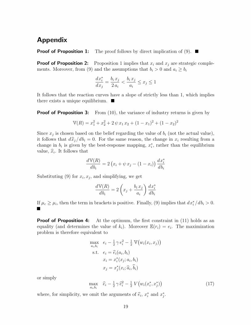
Proof of Proposition 1: The proof follows by direct implication of (9).

Proof of Proposition 2: Proposition 1 implies that xi

and x

j

are strategic comple-ments. Moreover, from (9) and the assumptions that b

i

> 0 and a

i

� b

i

dx

⇤i

dx

j

=b

i

x

j

2 ai

<

b

i

x

j

a

i

x

j

1

It follows that the reaction curves have a slope of strictly less than 1, which impliesthere exists a unique equilibrium.

Proof of Proposition 3: From (10), the variance of industry returns is given by

V(R) = x

21 + x

22 + 2 x1 x2 + (1� x1)

2 + (1� x2)2

Since xj

is chosen based on the belief regarding the value of bi

(not the actual value),it follows that dbx

j

/db

i

= 0. For the same reason, the change in x

i

resulting from achange in b

i

is given by the best-response mapping, x⇤i

, rather than the equilibriumvalue, bx

i

. It follows that

dV(R)

db

i

= 2�x

i

+ x

j

� (1� x

i

)�dx

⇤i

db

i

Substituting (9) for xi

, x

j

, and simplifying, we get

dV(R)

db

i

= 2

✓x

j

+b

i

x

j

a

i

◆dx

⇤i

db

i

If µc

� µ

i

, then the term in brackets is positive. Finally, (9) implies that dx⇤i

/db

i

> 0.

Proof of Proposition 4: At the optimum, the first constraint in (11) holds as anequality (and determines the value of k

i

). Moreover E(ri

) = e

i

. The maximizationproblem is therefore equivalent to

maxai,bi

e

i

� 12 � e

2i

� 12 V

�w

i

(xi

, x

j

)�

s.t. e

i

= bei

(ai

, b

i

)

x

i

= x

⇤i

(xj

; ai

, b

i

)

x

j

= x

⇤j

(xi

;bai

,

bb

i

)

or simplymaxai,bi

bei

� 12 � be

2i

� 12 V

�w

i

(x⇤i

, x

⇤j

)�

(17)

where, for simplicity, we omit the arguments of bei

, x⇤i

and x

⇤j

.

19

Consider the first-order condition with respect to b

i

. From (7), bei

is not a functionof b

i

or xi

. We thus focus on the partial derivative of V(wi

) with respect to b

i

as wellas the e↵ects through changes in x

i

.From (4) we see that @E(w

i

)/@xi

= 0. It follows that the first-order condition for(6) that corresponds to x

i

is equivalent to dV(wi

)/dxi

= 0. Given our assumptionthat bank i’s compensation contract is not observed by bank j’s CEO, it follows thatdx

⇤j

/db

i

= 0. In sum, the e↵ects through CEO portfolio choices are zero. It followsthat the first-order condition with respect to b

i

is simply given by

dV(wi

)

db

i

=@V(w

i

)

@ b

i

= 0

From (5), this first-order condition is given by

�a

i

x

i

� b

i

x

j

�x

j

� b

i

(1� x

j

)2 = 0

which leads to

b

i

= a

i

x

i

x

j

x

2j

+ (1� x

j

)2(18)

By the same argument as before, when computing the first-order condition withrespect to a

i

we can ignore the indirect e↵ects through x

i

and x

j

. We thus have

(1� �

i

e

i

)de

i

da

i

� 12

@V(wi

)

@a

i

= 0 (19)

From (7), ei

= a

i

/�

i

and de

i

/da

i

= 1/�i

. From (5)

@V(wi

)

@a

i

= 2 xi

�a

i

x

i

� b

i

x

j

�+ 2 a

i

(1� x

i

)2

Substituting the above equalities into (19) and simplifying, the first-order conditionwith respect to a

i

is given by

1� a

i

�

i

� x

i

�a

i

x

i

� b

i

x

j

�� a

i

(1� x

i

)2 = 0

Solving for ai

, we get

a

i

=1 + �

i

b

i

x

i

x

j

1 + �

i

x

2i

+ �

i

(1� x

i

)2(20)

Finally, (18) and (20) imply that ai

, b

i

> 0 for xi

, x

j

> 0.

Proof of Proposition 5: Symmetry implies that x

i

= x

j

= x and p

i

= p

j

= p,which in turn implies that (9) turns into

x = 12

�1 + p x

�

20

Solving for p we get

p =2 x� 1

x

(21)

The first-order condition with respect to the relative-performance parameter b

i

isgiven by

@V(wi

)

@ b

i

= 2 bi

x

2j

� 2 a

i

x

i

x

j

+ 2 bi

�1� x

j

�2= 0

At a symmetric equilibrium, this becomes

p = x

2

x

2 +(1� x)2(22)

Define

y ⌘ 1� x

x

(Note that x is striclty decreasing in y and that x 2 (12 , 1) implies that y 2 (0, 1).)Given this change in variable, (21) and (22) may be re-written as

1

p

=

1� y

1

p

=1 + y

2

(Note that either equation implies that p is strictly decreasing in y.) Together, theseequations imply

(1� y) (1 + y

2) =

2 (23)

Computation establishes that (23) has two imaginary roots and a real root. Setting = 0, the real root is y = 1, whereas setting = 1 we get y = 0. Moreover, thederivative of the left-hand side with respect to y is given by 1 + y (2� 3 y), which isstrictly positive for y 2 (0, 1), implying (by the implicit function theorem) that y isdecreasing in . Since p and x are increasing in y, it follows that p and x are strictlyincreasing in . Finally, from (23),

1� y

=

1 + y

2

It follows that1

p

=

1� y

=1 + y

2

>

1

where we use the fact that x 2 (0, 1) and thus y > 0. It follows that p < .

Proof of Proposition 6: The first-order condition with respect to b

i

implies:

�x

i

� p

i

x

j

�x

j

� p

i

(1� x

j

)2 = 0

21

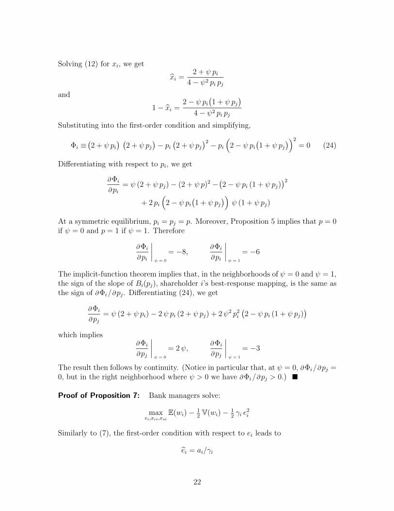
Solving (12) for xi

, we get

bxi

=2 + p

i

4�

2p

i

p

j

and

1� bxi

=2� p

i

�1 + p

j

�

4�

2p

i

p

j

Substituting into the first-order condition and simplifying,

�i

⌘�2 + p

i

� �2 + p

j

�� p

i

�2 + p

j

�2 � p

i

⇣2� p

i

�1 + p

j

�⌘2

= 0 (24)

Di↵erentiating with respect to p

i

, we get

@�i

@p

i

= (2 + p

j

)� (2 + p)2 ��2� p

i

(1 + p

j

)�2

+ 2 pi

⇣2� p

i

�1 + p

j

�⌘ (1 + p

j

)

At a symmetric equilibrium, pi

= p

j

= p. Moreover, Proposition 5 implies that p = 0if = 0 and p = 1 if = 1. Therefore

@�i

@p

i

���� = 0

= �8,@�

i

@p

i

���� = 1

= �6

The implicit-function theorem implies that, in the neighborhoods of = 0 and = 1,the sign of the slope of B

i

(pj

), shareholder i’s best-response mapping, is the same asthe sign of @�

i

/@p

j

. Di↵erentiating (24), we get

@�i

@p

j

= (2 + p

i

)� 2 p

i

(2 + p

j

) + 2 2p

2i

�2� p

i

(1 + p

j

)�

which implies@�

i

@p

j

���� = 0

= 2 ,@�

i

@p

j

���� = 1

= �3

The result then follows by continuity. (Notice in particular that, at = 0, @�i

/@p

j

=0, but in the right neighborhood where > 0 we have @�

i

/@p

j

> 0.)

Proof of Proposition 7: Bank managers solve:

maxei,xci,xsi

E(wi

)� 12 V(wi

)� 12 �i e

2i

Similarly to (7), the first-order condition with respect to e

i

leads to

bei

= a

i

/�

i

22

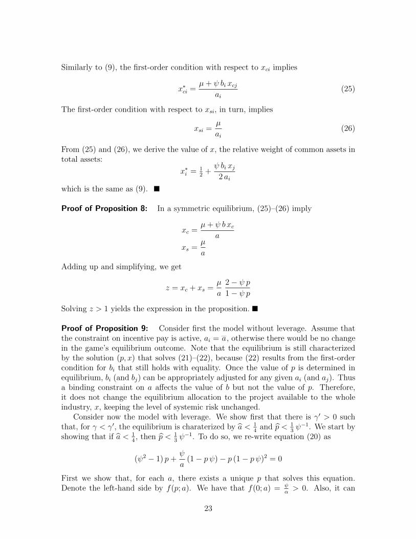
Similarly to (9), the first-order condition with respect to x

ci

implies

x

⇤ci

=µ+ b

i

x

cj

a

i

(25)

The first-order condition with respect to x

si

, in turn, implies

x

si

=µ

a

i

(26)

From (25) and (26), we derive the value of x, the relative weight of common assets intotal assets:

x

⇤i

= 12 +

b

i

x

j

2 ai

which is the same as (9).

Proof of Proposition 8: In a symmetric equilibrium, (25)–(26) imply

x

c

=µ+ b x

c

a

x

s

=µ

a

Adding up and simplifying, we get

z = x

c

+ x

s

=µ

a

2� p

1� p

Solving z > 1 yields the expression in the proposition.

Proof of Proposition 9: Consider first the model without leverage. Assume thatthe constraint on incentive pay is active, a

i

= a, otherwise there would be no changein the game’s equilibrium outcome. Note that the equilibrium is still characterizedby the solution (p, x) that solves (21)–(22), because (22) results from the first-ordercondition for b

i

that still holds with equality. Once the value of p is determined inequilibrium, b

i

(and b

j

) can be appropriately adjusted for any given a

i

(and a

j

). Thusa binding constraint on a a↵ects the value of b but not the value of p. Therefore,it does not change the equilibrium allocation to the project available to the wholeindustry, x, keeping the level of systemic risk unchanged.

Consider now the model with leverage. We show first that there is �0 > 0 suchthat, for � < �

0, the equilibrium is charaterized by ba <

14 and bp <

13

�1. We start byshowing that if ba <

14 , then bp <

13

�1. To do so, we re-write equation (20) as

( 2 � 1) p+

a

(1� p )� p (1� p )2 = 0

First we show that, for each a, there exists a unique p that solves this equation.Denote the left-hand side by f(p; a). We have that f(0; a) =

↵

> 0. Also, it can

23

be shown that the derivative of f with respect to p is everywhere negative (it hasa maximum at p = 2

3 �1, at which it is negative). Hence, if there is a zero of

f(p), it must be unique. Next we show that if a <

14 , then p <

13

�1. Evaluatingf(13

�1) = �1�4 a3 a � 13

27 �1. If a <

14 , then f(13

�1) < 0. With f(0) > 0, the zeroof the function must be such that p <

13

�1.Now we show that we can pick � small so that a <

14 if p <

13

�1. Consider now

equation (19) and assume that p <

13

�1. Note that 2�p

1�p

is increasing in p. Thus2�p

1�p

<

52 . The second term in the equilibrium condition

0 = (1� a) a21

�

� µ

2 2� p

1� p

is bounded between 2µ2 when p is zero and 5µ2/2 when p = 1

3 �1. A low enough �

increases the first term so that a has to decrease if the equality is to hold. Lower �means that less incentives need to be granted to induce the CEO to work equally ashard. (Note that (1 � a) a2 is increasing in a for a <

23 .) We conclude that there is

�

0> 0 such that for � < �

0, the equilibrium is characterized by a <

14 and p <

13

�1.Consider now the e↵ect of a cap on a when � < �

0. Assume that the constraint onincentive pay is active, which replaces the equilibrium condition (19). Use equation(20) and the implicit function theorem to get

@p

@a

=

a

2 (1� p )

� 2 1�a

a

� 2 + 4 p � 3 p2 2

If the denominator is negative, then @ p

@ a

< 0. When p <

13

�1, the denominator issuch that

�1� a

a

2 � 2 + 4 p � 3 p2 2< �1� a

a

2 � 2 + 4 13 � 3 p2 2

< 0

We’ve shown that for low enough �, @ p

@ a

< 0. Hence a cap on a causes p to increase.As a consequence, systemic risk increases. In fact,

x

⇤c

=µ

a (1� p)

and so

@x

⇤c

@a

= � µ

a

2 (1� p)+

µ

a (1� p)

@p

@a

= � µ

a (1� p)

✓1

a

�

@p

@a

◆

< 0

which concludes the proof.

24

Proof of Proposition 10: Suppose that E(w⇤i

) > v, where w

⇤i

corresponds to theunconstrained solution. Then the cap matters, that is, (21) holds as an equality.Consider first the model without leverage. Then (11) may be written as

maxai,bi

e

i

� v

subject to the participation constraint,

v � 12 V(wi

)� d

i

(ei

) � u

i

as well as the constraint that ei

and x

i

belong to the best-response mappings.Notice that b

i

is not present in the objective function: from (7), ei

is a function ofa

i

but not bi

. It follows that the optimal bi

maximizes the slack in the participationconstraint. As shown in the proof of Proposition 4, this implies @V(w

i

)/@ bi

= 0,which in turn determines the value of p

i

= a

i

/b

i

. It follows that the same value of pi

obtains as in the problem without the condition (21).Consider now the model with leverage. The problem faced by shareholders is:

maxki,ai,bi

E(ri

� w

i

)

subject to

E(wi

)� 12 V(wi

)� d

i

(ei

) � u

i

E(wi

) = v

and that ei

and x

c

and x

s

belong to the best-response functions. Let ki

be such thatE(w

i

) = v and rewrite the problem as:

maxai,bi

E(ri

)� v

subject tov � 1

2 V(wi

)� 12 �

�1i

a

2i

� u

i

(27)

Letting � � 0 be the Lagrange multiplier associated with the constraint, we have

maxai,bi

E(ri

) + �

⇣v � 1

2 V(wi

)� 12 �

�1i

a

2i

� u

i

⌘

Notice that this problem has the same solution to the unconstrained problem

maxai,bi

E(ri

)� 12 V(w

i

)� 12 �

�1i

a

2i

� u

i

if � = 1.We start by evaluating � when the constraint on pay is just binding, i.e., E(w⇤

i

) =v. Use the constraint (27) (with equality) to get implicitly the value of a given b,a = f(b; v), and use the first order condition w.r.t. a to get the value of �:

� =dE(r

i

)/da

�

�1i

a

i

=1

a

i

� �

2� p

1� p

µ

2

a

3i

25

where we have used the equilibrium solution for x

c

and assumed symmetry. Whenthe cap on pay is just binding, equation (19) holds we get that � = 1. Now compute

d�

da

=@�

@a

+@�

@p

dp

da

= � 1

a

2i

+ 3 �2� p

1� p

µ

2

a

4i

� �

(1� p )2µ

2

a

3i

dp

da

To evaluate the last term, use the implicit function theorem to get

df

db

= �12 @V(wi

)/@ b12 @V(wi

)/@a+ �

�1i

a

i

Below we show that @V(wi

)/@a = 0 and from the first order condition w.r.t. b, itcan be shown that @V(w

i

)/@ b > 0.11 Thus

dp

da

=1

a

db

da

� p

a

< 0

When the cap on pay is just binding, The sum of the two first terms in d�/da ispositive and so d�/da > 0.

Consider now a cap that is infinitesimally below E(w⇤i

). It must be that theLagrange multiplier on the constraint (27) increases, since we are below the uncon-strained optimum. Because d�/da > 0, to achieve an increase in � while at the sametime trading o↵ b and a so as to keep constraint (27) with equality,a must increaseand b decrease. Hence p decreases. Overall, systemic risk is reduced.

To conclude the proof, we show that @V(wi

)/@ai

= 0. We know that

V(wi

) = a

2i

x

2ci

+ b

2i

x

2cj

� 2ai

b

i

x

ci

x

cj

+ a

2i

x

2si

+ b

2i

x

2sj

a

i

x

⇤ci

= µ+ b

i

x

cj

x

⇤si

=µ

a

i

e

⇤i

= a

i

/�

i

Therefore,

@V(wi

)

@a

i

= 2 ai

x

2ci

� 2 b

i

x

ci

x

cj

+ 2 ai

x

2si

�2 a2i

x

ci

µ+ b

i

x

cj

a

2i

+ 2 a

i

b

i

x

cj

µ+ b

i

x

cj

a

2i

� 2 a2i

x

si

µ

a

2i

which, after replacing the equilibrium values for xci

and x

si

, gives the desired result.

11. The first order condition w.r.t. b yields:

µ

dx

c

db

� �

1

2

dV(wi

)

db

= 0

If � � 0 and dxcdb

= xcj

a

> 0, then dV(wi)db

� 0.

26

References

Acharya, V., Mehran, H., and Thakor, A. “Caught between Scylla andCharybdis? Regulating Bank Leverage When There Is Rent Seeking and RiskShifting.” Review of Corporate Finance Studies, (2015).

Acharya, V.V. “A Theory of Systemic Risk and Design of Prudential BankRegulation.” Journal of Financial Stability, Vol. 5 (2009), pp. 224–255.

Acharya, V.V. and Volpin, P.F. “Corporate Governance Externalities.”Review of Finance, Vol. 14 (2010), pp. 1–33.

Acharya, V.V. and Yorulmazer, T. “Information Contagion and BankHerding.” Journal of Money, Credit and Banking, Vol. 40 (2008), pp. 215–231.

Admati, A. and Hellwig, M. The Bankers’ New Clothes: What’s Wrong With

Banking and What to Do About It. Princeton University Press, 2013.

Albuquerque, A. “Peer firms in relative performance evaluation.” Journal of

Accounting and Economics, Vol. 48 (2009), pp. 69–89.

Albuquerque, A.M. “Do Growth-Option Firms Use Less Relative PerformanceEvaluation?” The Accounting Review, Vol. 89 (2014), pp. 27–60.

Allen, F., Babus, A., and Carletti, E. “Asset commonality, debt maturityand systemic risk.” Journal of Financial Economics, Vol. 104 (2012), pp. 519–534.

Angelis, D.D. and Grinstein, Y. “Relative Performance Evaluation in CEOCompensation: A Non-Agency Explanation.” Available at SSRN 2432473 (2016).

Asai, K. “Is Capping Executive Bonuses Useful?” Imf working paper (2016).

Barakova, I. and Palvia, A. “Limits to relative performance evaluation:evidence from bank executive turnover.” Journal of Financial Economics Policy,Vol. 2 (2010), pp. 214–236.

Barro, J. and Barro, R. “Pay, performance and turnover of bank CEOs.”Journal of Labor Economics, Vol. 8 (1990), pp. 448–481.

Bhagat, S., Bolton, B., and Romano, R. “The Promise and Peril ofCorporate Governance Indices.” Columbia Law Review, (2008), pp. 1803–1882.

Bhattacharyya, S. and Purnanandam, A. “Risk-taking by Banks: What Didwe Know and When Did we Know It?” AFA 2012 Chicago Meetings Paper(2011).

Bizjak, J., Kalpathi, S., Li, Z., and Young, B. “The role of peer firmselection in explicit relative performance awards.” Working paper (2016).

27

Bolton, P., Mehran, H., and Shapiro, J. “Executive compensation and risktaking.” Review of Finance, (2015), pp. 1–43.

Chaigneau, P. “Risk-shifting and the regulation of bank CEOs compensation.”Journal of Financial Stability, (2012).

Cheng, I.H. “Corporate Governance Spillovers.” Dartmouth college (2011).

Crawford, A. “Relative performance evaluation in CEO pay contracts: evidencefrom the commercial banking industry.” Managerial Finance, Vol. 25 (1999), pp.34–54.

Dicks, D.L. “Executive Compensation and the Role for Corporate GovernanceRegulation.” Review of Financial Studies, (2012).

Farhi, E. and Tirole, J. “Collective Moral Hazard, Maturity Mismatch, andSystemic Bailouts.” American Economic Review, Vol. 102 (2012), pp. 60–93.

Ferrarini, G. “CRD IV and the mandatory structure of bankers’ pay.” Ecgi lawworking paper no. 289 (2015).

French, K.R., Baily, M.N., Campbell, J.Y., Cochrane, J.H., Diamond,D.W., Duffie, D., Kashyap, A.K., Mishkin, F.S., Rajan, R.G.,Scharfstein, D.S., Shiller, R.J., Shin, H.S., Slaughter, M.J., Stein,J.C., and Stulz, R.M. The Squam Lake Report Fixing the Financial System.Princeton University Press, 2010.

Geithner, T. “Statement of Treasury Secretary Geithner to the SenateSubcommittee of the Committee on Appropriations, 111th Congress.” Financialservices and general government appropriations for fiscal year 2010, 16-17, u.s.government printing o�ce, washington, dc. (2010).

Hauswald and Senbet. “Executive compensation, supervisory incentives andbanking regulation.” Working paper (2009).

Hilscher, J., Landskroner, Y., and Raviv, A. “Optimal regulation, executivecompensation and risk taking by financial institutions.” Working paper (2016).

Holmstrom, B. “Moral Hazard and Observability.” Bell Journal of Economics,Vol. 10 (1979), pp. 74–91.

Ilic, D., Pisarov, S., and Schmidt, P. “Preaching water but drinking wine?Relative performance evaluation in International Banking.” University of zurichworking paper # 208 (2015).

International Monetary Fund. “Global Financial Stability Report.”Technical report (2014).

28

Kane, E. “Redefining and containing systematic risk.” Working paper (2010).

Kleymenova, A. and Tuna, I. “Regulation of compensation.” Working paper(2015).

Kolm, J., Laux, C., and Loranth, G. “Regulating bank CEO compensationand active boards.” Working paper (2014).

Levit, D. and Malenko, N. “The Labor Market for Directors and Externalitiesin Corporate Governance.” Journal of Finance, Vol. 71 (2016), pp. 775–808.

Martinez-Miera, D. and Suarez, J. “Banks’ endogenous systemic risktaking.” Working paper (2014).

Murphy, K.J. “Compensation Structure and Systemic Risk.” Marshall researchpaper series working paper fbe 34-09 (2009).

—. “Regulating Banking Bonuses in the European Union: a Case Study inUnintended Consequences.” European Financial Management, Vol. 19 (2013), pp.631–657.

Ozdenoren, E. and Yuan, K. “Endogenous Contractual Externalities.” Lbs andlse (2014).

Posner, R.A. A Failure of Capitalism: The Crisis of ’08 and the Descent into

Depression. Harvard University Press, 2009.

Thanassoulis, J. “The Case for Intervening in Bankers’ Pay.” Journal of

Finance, Vol. 67 (2012), pp. 849–894.

—. “Bank Pay Caps, Bank Risk, and Macroprudential Regulation.” Journal of

Banking & Finance, Vol. 48 (2014), pp. 139–151.

Zwiebel, J. “Corporate Conservatism and Relative Compensation.” Journal of

Political Economy, Vol. 103 (1995), pp. 1–25.

29