Embed Size (px)
Citation preview

Relative Navigation of Air Vehicles
Adam M. Fosbury∗
Air Force Research Laboratory, Space Vehicles Directorate, Kirtland Air Force Base, NM 87117
John L. Crassidis†
University at Buffalo, State University of New York, Amherst, NY 14260-4400
This paper derives the full equations of motion for relative navigation
of air vehicles. An extended Kalman filter is used for estimating the rela-
tive position and attitude of two air vehicles, designated leader and follower.
All leader states are assumed known, while the relative states are estimated
using line-of-sight measurements between the vehicles along with accelera-
tion and angular rate measurements of the follower. Noise is present on all
measurements, while biases are present only on the latter two. The global
attitude is parameterized using a quaternion, while the local attitude error
is given by a three-dimensional attitude representation. An application of
the new theoretical developments is also given, which involves determining
an optimal trajectory to improve the estimation accuracy of the system. A
cost function is derived based upon the relative position elements of the
estimator covariance. State constraints are appended to the cost function
using an exponential term. Results show that minimization of this cost
function yields a trajectory that improves accuracy of both the position
and attitude state estimates.
I. Introduction
Formation flight of aircraft has been an active and growing area of study in recent years.
With the advent of cheaper sensors, especially micro-mechanical ones,1 several new applica-
tions including uninhabited air vehicles (UAVs) have become mainstream. Most applications
∗Aerospace Engineer. Email: [email protected]. Member AIAA.†Professor, Department of Mechanical & Aerospace Engineering, Email: [email protected]. Asso-
ciate Fellow AIAA.
1 of 28
of UAVs involve military operations, some of which include reconnaissance, electronic war-
fare, and battle damage assessment. It is expected that thirty percent of the Air Force aircraft
will be pilotless by the year 2010.2 This growth is expected to yield a more integrated UAV
arsenal capable of detection and elimination of enemy targets. Numerous civilian applica-
tions have been envisioned for the future including border interdiction, search and rescue,
wild fire suppression, communications relays, law enforcement, and disaster and emergency
management.3 Cooperative UAV formations will play an important role in both military
and civil applications for simultaneous coordination of resources over large areas.
Relative navigation of air vehicles flying in a formation is essential to meet mission
objectives. The most common navigation mechanism for air vehicles involves the integration
of Global Positioning System (GPS) signals with Inertial Measurement Units (IMUs). Both
position and attitude information is possible using this type of inertial navigation system,
however it requires that each vehicle must have the full GPS/IMU sensor complement. This
also provides absolute information, which must be converted to relative coordinates using
appropriate transformations. The relative information is often required for formation control
applications and coordination.4
Recent investigations involve developing navigation systems without the use of GPS
satellites, because the GPS signal is highly susceptible to conventional interference as well
as intentional jamming and spoofing. Vision-based approaches have been developed for this
purpose, which can be used for both relative and absolute navigation. These approaches have
the advantage of not relying on external sensors, however they require considerable onboard
computation.5 Reference 6 demonstrates a vision-based method of formation control and
state estimation. Two approaches are used. The first incorporates an extended Kalman
filter (EKF) developed in Ref. 7 with camera-based images to determine the relative states.
The second approach uses image size and location to directly regulate the control algorithm.
Results indicate that relative navigation is possible with a single camera.
By far the primary mechanism historically used to blend GPS measurements with IMU
data has been the EKF.8 Other implementations include an unscented Kalman filter9 and
particle filters.10 The earliest known discussion on the use of GPS with IMUs for relative
navigation occurs in Ref. 11. Relative position is propagated using a linear discrete equation,
though the exact form of the state transition matrix is not provided. Increased accuracy is
achieved due to the high correlation of GPS measurements between the leader and follower.
These results have also been extended to vehicle platooning.12
In all the aforementioned papers, simplified models are used for the air vehicle dynamics.
These may be adequate for a particular application, but having the full navigation equations
can provide insights to the validity of using the simplified models. Deriving the full navigation
equations, as well as the subsequent Kalman filter expressions, is the main purpose of the
2 of 28
work presented in this paper. The relative attitude kinematics between two vehicles is well
known.13 Here, the full relative position equations including gravity models are also derived.
An EKF is used for state estimation. Relative measurements involving line-of-sight (LOS)
observations between the air vehicles are used, thus freeing the system from external sensors
such as GPS. A minimum of three LOS observations are required for effective and accurate
state estimation, even in the face of multiple initial condition errors.14 Biased gyro and
accelerometer measurements are also assumed for the follower air vehicle in order to provide
full filtered position and attitude estimation.
One method for measuring LOS observations between multiple vehicles is the vision-based
navigation (VISNAV) system.15 This consists of an optical sensor combined with a specific
light source (beacon) in order to achieve a selective vision. The VISNAV system is applied
to the spacecraft formation flying problem in Ref. 16. State estimation is performed using an
optimal observer design. Simulations show that accurate estimates of relative position and
attitude are possible. An EKF is applied to the VISNAV-based relative spacecraft position
and attitude estimation in Ref. 17. Automatic refueling of UAVs using a VISNAV-based
system is shown in Refs. 18 and 19. Here, we focus on using the fully derived relative
equations for relative air vehicle navigation.
Optimal control techniques are widely used for trajectory optimization of dynamic sys-
tems. These types of problems generally require the solution of two-point boundary value
problems through use of numerical methods. An optimal control law has been designed to
improve range estimation accuracy between two vehicles.20 Motion of the system is confined
to two dimensions. Components of the EKF covariance matrix are used for the cost function.
This paper examines a similar cost function to determine whether the estimation accuracy
of the EKF can be improved by following a specific relative trajectory.
The organization of this paper is as follows. A summary of the various coordinate frames
used in this work is first provided. This is followed by a review of quaternion attitude param-
eters and the associated kinematics. The relative navigation equations are then developed.
Next, an EKF for relative state estimation is reviewed, followed by the derivation of mea-
surement equations. Simulation results are shown using a calibration maneuver to determine
the gyro and accelerometer biases. Then an application of the relative navigation theory is
shown, where a cost function is developed to minimize the position components of the state
error-covariance matrix. Simulation results are also provided showing the effectiveness of
the optimal control law.
3 of 28
Prime
Meridian
Plane
Equatorial
Plane2e
3 3ˆ ˆ,i e
n
e
1e
dr
1i2i
Inertial
Reference
Direction
Figure 1. Definitions of Various Reference Frames
II. Reference Frames
This section summarizes the various reference frames used in the remainder of this paper,
as shown in Figure 1:
• Earth-Centered-Inertial (ECI): denoted by i1, i2, i3. The origin is at the center of
the Earth, with the i1 axis pointing in the direction of the vernal equinox, the i3
axis pointing towards the geographic North pole, while i2 completes the right-handed
coordinate system. Vectors defined in this frame are identified by the letter I.
• Earth-Centered-Earth-Fixed (ECEF): denoted by e1, e2, e3. The origin of this frame
is also located at the center of the Earth. The primary difference is that this frame
rotates with the Earth. The e3 axis points towards the north pole and is equal to i3.
The e1 axis is directed toward the prime meridian, and the e2 axis completes the right-
handed system. The letter E signifies a vector defined with respect to this reference
frame.
• North-East-Down (NED): denoted by n, e, d. This reference frame is commonly
used for inertial navigation and is formed by fitting a tangent plane to the geodetic
reference ellipse at a given point of interest.21 The n axis points North, the e axis is
directed East, and the d axis completes the right-handed system. This reference frame
is generally used for local navigation purposes. The letter N signifies a vector defined
4 of 28
with respect to this reference frame. A thorough discussion on the conversion between
the NED and ECEF frames can be found in Ref. 21.
• Body Frames: denoted by b1, b2, b3. These are fixed to the vehicle body, rotating
with it. Body frames fixed to the two air vehicles are designated leader (l) and follower
(f). The letter B signifies a vector defined with respect to a generic body frame.
The convention applied in this paper is to use these letters as a superscript following the
vector or matrix that is being described.
III. Attitude Kinematics
A variety of parameterizations can be used to specify attitude, including Euler angles,
quaternions, and Rodrigues parameters.22 This paper uses the quaternion, which is based
on the Euler angle/axis parameterization. The quaternion is defined as q ≡ [ T q4 ]T with
= [ q1 q2 q3 ]T = e sin(ν/2), and q4 = cos(ν/2), where e and ν are the Euler axis of
rotation and rotation angle, respectively. This vector must satisfy the constraint qTq = 1.
The attitude matrix can be written as a function of the quaternion:
A = ΞT (q)Ψ(q) (1)
where
Ξ(q) ≡
q4I3×3 + [×]
−T
(2a)
Ψ(q) ≡
q4I3×3 − [×]
−T
(2b)
with
[×] =
0 −q3 q2
q3 0 −q1
−q2 q1 0
(3)
The attitude kinematic equation is given by23
ABI = −[ωB
B|I×]ABI (4)
where ωBB|I is the angular velocity of the body frame with respect to the inertial frame, given
in body frame coordinates, and ABI is the attitude matrix that converts vectors from the
5 of 28
inertial frame to the body frame.
The relative quaternion qf |l and corresponding attitude matrix are defined by
qf |l ≡ qf ⊗ q−1l (5a)
Afl ≡ A(qf |l) = A(qf )A
T (ql) (5b)
which are consistent with Refs. 22 and 24. The symbol ⊗ denotes quaternion multiplication,
given by
qa ⊗ qb ≡[
Ψ(qa) qa
]
qb =[
Ξ(qb) qb
]
qa (6)
and q−1 is the quaternion inverse, defined by q−1 ≡ [− q4]T .
Reference 13 shows the relative quaternion kinematics to be given by
qf |l =1
2Ξ(qf |l)ω
f
f |l (7)
where ωf
f |l is the relative angular velocity defined as
ωf
f |l ≡ ωf
f |E − Afl ω
ll|E (8)
To reduce the computational load, a discrete form of the quaternion propagation is used.
This is given by13
qf |lk+1= Ω(ωf
fk)Γ(ωl
lk)qf |lk (9)
where
Ω(ωffk
) ≡
cos(
12‖ωf
fk‖∆t
)
I3×3 − [ψk×] ψk
−ψTk cos
(
12‖ωf
fk‖∆t
)
(10a)
ψk ≡sin(
12‖ωf
fk‖∆t
)
ωffk
‖ωffk‖
(10b)
Γ(ωllk) ≡
cos(
12‖ωl
lk‖∆t
)
I3×3 − [ζk×] −ζk
ζTk cos
(
12‖ωl
lk‖∆t
)
(10c)
ζk ≡sin(
12‖ωl
lk‖∆t
)
ωllk
‖ωllk‖
(10d)
and ∆t is the sampling interval.
6 of 28
IV. Relative Position Equations
The relative position equations to be used in the EKF are developed in this section with
the relative position vector defined as
rf
f |l = rf
f |I − Afl r
ll|I
= AfI (r
If |I − rI
l|I) (11)
Taking two time derivatives yields
rf
f |l =d2
dt2
(
rf
f |l
)
=d2
dt2
(
AfI
)
(rIf |I − rI
l|I) + 2d
dt
(
AfI
) d
dt(rI
f |I − rIl|I) + Af
I
d2
dt2(
rIf |I − rI
l|I
)
= −(
[(ωf
f |I)×] + [(ωf
f |I)×][(ωf
f |I)×])
AfI r
If |l − 2[(ωf
f |I)×]AfI r
If |l + Af
I
(
rIf |I − rI
l|I
)
= −ωf
f |I × rf
f |l − [(ωf
f |I)×][(ωf
f |I)×]rf
f |l − 2ωf
f |I × rf
f |l + AfI
(
rIf |I − rI
l|I
)
(12)
The inertial accelerations of the leader and follower are given by Newton’s law:
rIl|I = aI
l + gIl (13a)
rIf |I = aI
f + gIf (13b)
The gravity model in ECEF coordinates is given by
gE =−µ
‖rE‖3rE (14)
where µ = 3.986×10¹⁴ m3/(kg−s2). Equation (14) provides the only nonlinear term in the
relative acceleration. Equation (12) is then written as
rf
f |l = −ωf
f |I × rf
f |l − [(ωf
f |I)×][(ωf
f |I)×]rf
f |l − 2ωf
f |I × rf
f |l + AfI
(
aIf − aI
l
)
+ AfE
(
gEf − gE
l
)
(15)
The acceleration measurement model is defined as
aff = a
ff + bfa + ηfav (16a)
bfa = ηfau (16b)
where bfa is the accelerometer bias, and ηfav and ηfau are zero-mean Gaussian white noise
processes. Their respective spectral densities are σ2avI3×3 and σ2
auI3×3.
7 of 28
The gyro measurement model has a similar form:
ωf
f |I = ωf
f |I + bfg + ηfgv (17a)
bfg = ηfgu (17b)
where bfg is the gyro bias, and ηfgv and ηfgu are zero-mean Gaussian white noise processes
with spectral densities σ2gvI3×3 and σ2
guI3×3. See the appendix of Ref. 25 for a more detailed
discussion on the gyro bias model.
V. Extended Kalman Filter Equations
The states of interest in this EKF are relative attitude, relative position, relative velocity,
and biases on the inertial acceleration and angular velocity measurements:
x =[
qTf |l (rf
f |l)T (rf
f |l)T bT
fg bTfa
]T
(18)
The following estimate equations are based on the truth equations of the prior sections:
˙qf |l =1
2Ξ(qf |l)ω
f
f |l (19a)
¨rf
f |l = − ˙ωf
f |I × rf
f |l − [(ωf
f |I)×][(ωf
f |I)×]rf
f |l − 2ωf
f |I ×˙rf
f |l + AfI
(
aIf − aI
l
)
+ AfE
(
gEf − gE
l
)
(19b)
aff = a
ff − bfa (19c)
gEf =
−µ
‖rEf |E‖
3rE
f |E (19d)
ωf
f |I = ωf
f |I − bfg (19e)
˙bfa = 0 (19f)
˙bfg = 0 (19g)
The state-error vector is given as
∆x =[
δαTf |l (∆r
f
f |l)T (∆r
f
f |l)T ∆bT
fg ∆bTfa
]T
(20)
The first term is defined by
δαf |l = 2δf |l (21a)
δqf |l = qf |l ⊗ q−1f |l (21b)
8 of 28
where δαf |l corresponds to a vector of half-error angles for any small roll, pitch and yaw
sequence, and δf |l denotes the first three components of the four component vector δqf |l.
The usual EKF assumption that the estimate is close, to within first-order dominate terms,
to the truth is applied. For this case, the fourth error-component is approximately one
and its derivative is near zero.24 The remaining state-error terms are defined generically as
∆y = y − y, while the process noise vector consists of the four Gaussian noise terms from
the measurement equations:
w =[
ηTfgv ηT
fgu ηTfav ηT
fau
]T
(22)
The next step is to determine time derivatives of the error states. The equation for δαf |l
is given in Ref. 26 as
δαf |l = −[(ωf
f |l)×]δαf |l + δωf
f |l (23)
where
δωf
f |l = ωf
f |l − ωf
f |l (24)
Based upon the definitions in Eqs. (8) and (17a), along with the approximation
Afl = (I3×3 − [(δαf |l)×])Af
l (25)
Eq. (24) becomes
δωf
f |l = −∆bfg − ηfgv − [(Afl ω
ll|I)×]δαf |l (26)
Equation (23) then simplifies to
δαf |l = −[(ωf
f |I)×]δαf |l − ∆bfg − ηfgv (27)
The time derivative of the position error-state vector is simply equal to the velocity error
state vector:d
dt(∆r
f
f |l) = ∆rf
f |l (28)
The time derivative of the velocity vector is more complicated. To keep this paper concise,
the algebraic derivation of this equation will be omitted. The final result makes use of several
of the relations already mentioned in this paper, along with Euler’s equation23
ωf
f |I = J−1f
(
uf − [(ωf
f |I)×]Jfωf
f |I
)
(29)
where Jf is the inertia matrix of the follower and uf is the applied torque. An expansion of
9 of 28
the gravity model in Eq. (14) is also required:
gEf = gE
f +∂gE
f
∂∆rf
f |l
∆rf
f |l +∂gE
f
∂δαf |l
δαf |l (30)
where
∂gEf
∂∆rf
f |l
= −µAEf ‖r
El|I + AE
f rf
f |l‖−3
+3µ(
rEl|I + AE
f rf
f |l
)(
rEl|I + AE
f rf
f |l
)T
‖rEl|I + AE
f rf
f |l‖−5 (31)
∂gEf
∂δαf |l
= −µAEf [(rf
f |l)×]‖rEl|I + AE
f rf
f |l‖−3
+3µ(
rEl|I + AE
f rf
f |l
)(
rEl|I + AE
f rf
f |l
)T
AfE[(rf
f |l)×]‖rEl|I + Af
E rf
f |l‖−5 (32)
Using the above relations, the velocity error-dynamics equation is written as
d
dt∆r
f
f |l = F3−1δαf |l + F3−2∆rf
f |l + F3−3∆rf
f |l + F3−4∆bfg
+ F3−5∆bfa + G3−1ηfgv + G3−3ηfav
(33)
10 of 28
where
F3−1 = − [(Afl a
ll)×] + [(Af
E
(
gEf − gE
l
)
)×] − µAfE
AEf [(rf
f |l)×]‖rEl|I + AE
f rf
f |l‖−3
−3(
rEl|I + AE
f rf
f |l
)(
rEl|I + AE
f rf
f |l
)T
AEf [(rf
f |l)×]‖rEl|I + AE
f rf
f |l‖−5
(34a)
F3−2 = − [(ωf
f |I)×][(ωf
f |I)×] − [( ˙ωf
f |I)×] − µAfE
AEf ‖r
El|I + AE
f rf
f |l‖−3
− 3(
rEl|I + AE
f rf
f |l
)(
(rEl|I)
T + (AEf r
f
f |l)T)
‖rEl|I + AE
f rf
f |l‖−5 (34b)
F3−3 = −2[(ωf
f |I)×] (34c)
F3−4 = − [(rf
f |l)×]J−1f
[(Jf ωf
f |I)×] − [(ωf
f |I)×]Jf
− 2[( ˙rf
f |l)×]
−(
[(ωf
f |I × rf
f |l)×] + [(ωf
f |I)×][(rf
f |l)×]) (34d)
F3−5 = −I3 (34e)
G3−1 = − [(rf
f |l)×]J−1f
[(Jf ωf
f |I)×] − [(ωf
f |I)×]Jf
− 2[( ˙rf
f |l)×]
−(
[(ωf
f |I × rf
f |l)×] + [(ωf
f |I)×][(rf
f |l)×]) (34f)
G3−3 = −I3 (34g)
Lastly, the time derivatives of the bias states are found by using Eqs. (16b) through (17b):
∆bfa = ηfau (35a)
∆bfg = ηfgu (35b)
The overall error dynamics are governed by the equation
∆x = F∆x + Gw (36)
where the F and G matrices are given by
F =
−[(ωf
f |I)×] 03×3 03×3 −I3×3 03×3
03×3 03×3 I3×3 03×3 03×3
F3−1 F3−2 F3−3 F3−4 F3−5
03×3 03×3 03×3 03×3 03×3
03×3 03×3 03×3 03×3 03×3
(37)
11 of 28
G =
−I3×3 03×3 03×3 03×3
03×3 03×3 03×3 03×3
G3−1 03×3 G3−3 03×3
03×3 I3×3 03×3 03×3
03×3 03×3 03×3 I3×3
(38)
The process noise covariance matrix used in the EKF is
Q =
σ2fgvI3×3 03×3 03×3 03×3
03×3 σ2fguI3×3 03×3 03×3
03×3 03×3 σ2favI3×3 03×3
03×3 03×3 03×3 σ2fauI3×3
(39)
A discrete propagation is used for the covariance matrix in order to reduce the compu-
tational load:
P−k+1 = ΦkP
+k ΦT
k + Qk (40)
where Φk is the state transition matrix and Qk is the covariance matrix. Reference 27 gives
a numerical solution for these matrices. The first step is to set up the following 2n by 2n
matrix:
A =
−F GQGT
0n×n F T
∆t (41)
The matrix exponential is then calculated:
B = eA =
B11 B12
0n×n B22
=
B11 Φ−1k Qk
0n×n ΦTk
(42)
The state transition and covariance matrices are then given as
Φk = BT22 (43a)
Qk = ΦkB12 (43b)
Note that Eq. (41) is only valid for constant system and covariance matrices. However,
for small ∆t it is a good approximation of the actual discrete-time matrices that are time
varying.
12 of 28
Leader
Follower
Beacon
(Xi, Yi, Zi)
(x, y, z)
(Xi+x, Yi+y, Zi+z)
||(Xi+x, Yi+y, Zi+z)||
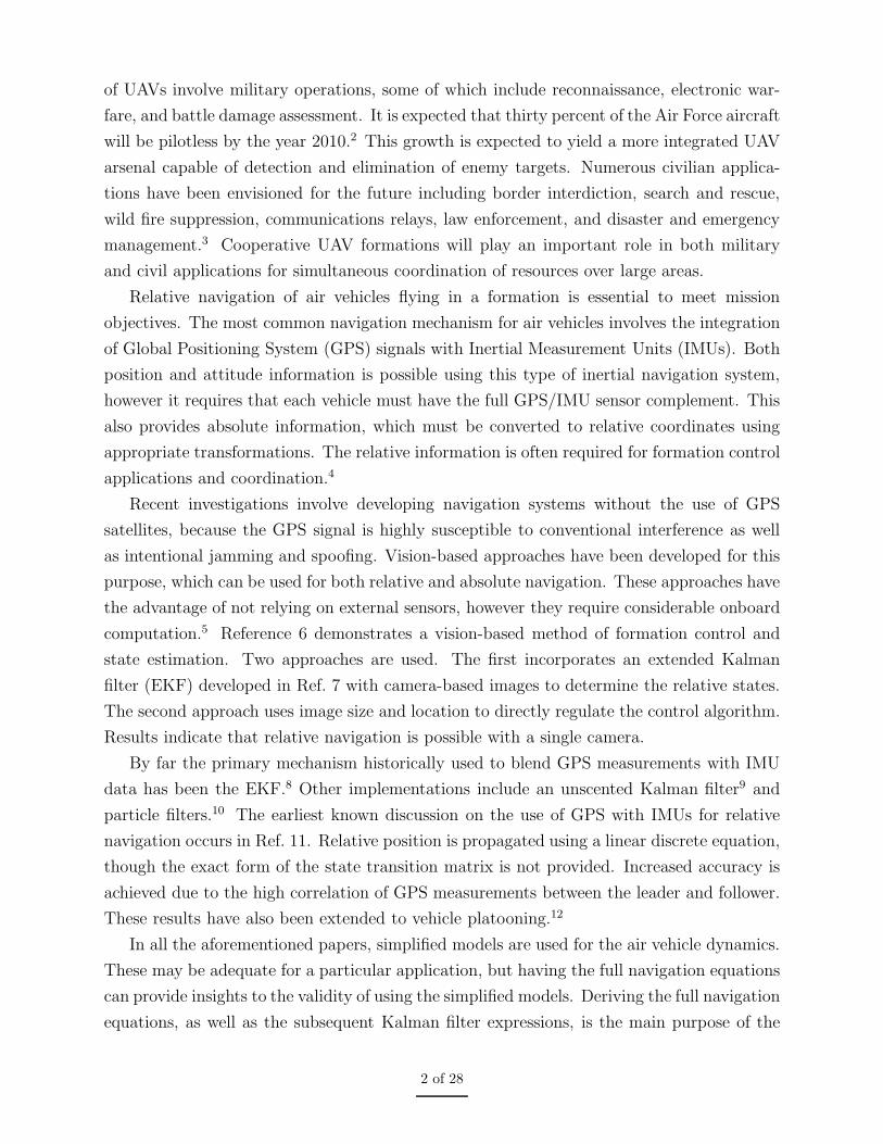
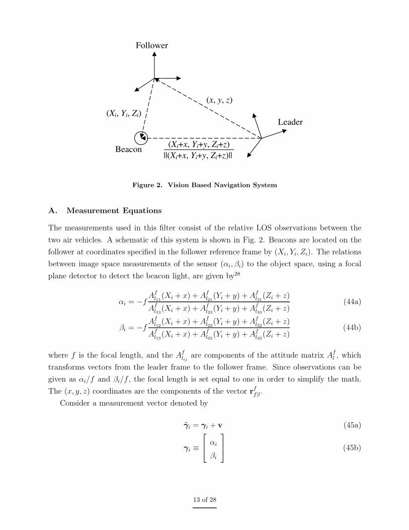
Figure 2. Vision Based Navigation System
A. Measurement Equations
The measurements used in this filter consist of the relative LOS observations between the
two air vehicles. A schematic of this system is shown in Fig. 2. Beacons are located on the
follower at coordinates specified in the follower reference frame by (Xi, Yi, Zi). The relations
between image space measurements of the sensor (αi, βi) to the object space, using a focal
plane detector to detect the beacon light, are given by28
αi = −fAf
l11(Xi + x) + Af
l21(Yi + y) + Af
l31(Zi + z)
Afl13
(Xi + x) + Afl23
(Yi + y) + Afl33
(Zi + z)(44a)
βi = −fAf
l12(Xi + x) + Af
l22(Yi + y) + Af
l32(Zi + z)
Afl13
(Xi + x) + Afl23
(Yi + y) + Afl33
(Zi + z)(44b)
where f is the focal length, and the Aflij
are components of the attitude matrix Afl , which
transforms vectors from the leader frame to the follower frame. Since observations can be
given as αi/f and βi/f , the focal length is set equal to one in order to simplify the math.
The (x, y, z) coordinates are the components of the vector rf
f |l.
Consider a measurement vector denoted by
γi = γi + v (45a)
γi ≡
αi
βi
(45b)
13 of 28

A frequently used covariance of v is given by Ref. 29 as
RFOCALi =
σ2
1 + d(α2i + β2
i )
(1 + dα2i )
2 (dαiβi)2
(dαiβi)2 (1 + dβ2
i )2
(46)
where d is on the order of 1 and σ is assumed to be known. Note that the components of this
covariance matrix will increase as the image space coordinates increase. This demonstrates
that errors will increase as the observation moves away from the boresight. Reference 29 also
states that for practical purposes, the estimated values of αi and βi must be used in place
of the true quantities. This only leads to second-order error effects.
The problem with using Eq. (45a) as the measurement vector is that the definitions of
αi and βi in Eq. (44) are highly nonlinear in both the position and attitude components. A
simpler observation vector is given in unit vector form as
bi = (Afl )
T ri (47a)
ri ≡Ri + r
f
f |l
‖Ri + rf
f |l‖(47b)
where Ri = [ Xi Yi Zi ]T , rf
f |l ≡ [ x y z ]T , and for a sensor facing in the positive Z
direction,
bi =1
√
1 + α2i + β2
i
−αi
−βi
1
(48)
Similar equations for the positive X and Y directions are found by rotating the elements of
the vector in a cyclic manner. Sensors facing in the negative direction use the same equations
multiplied by −1.
The QUEST measurement model shown in Ref. 30 works well for small field-of-view
sensors, but may produce significant errors for larger field of views, such as the VISNAV
sensor. A new covariance model is developed in Ref. 31 that provides better accuracy than
the QUEST model for this case. It is based upon a first-order Taylor series expansion of
the unit vector observation. The primary assumption is that the measurement noise is small
compared to the signal. The new covariance is defined as
RNEWi = JiR
FOCALi JT
i (49)
14 of 28
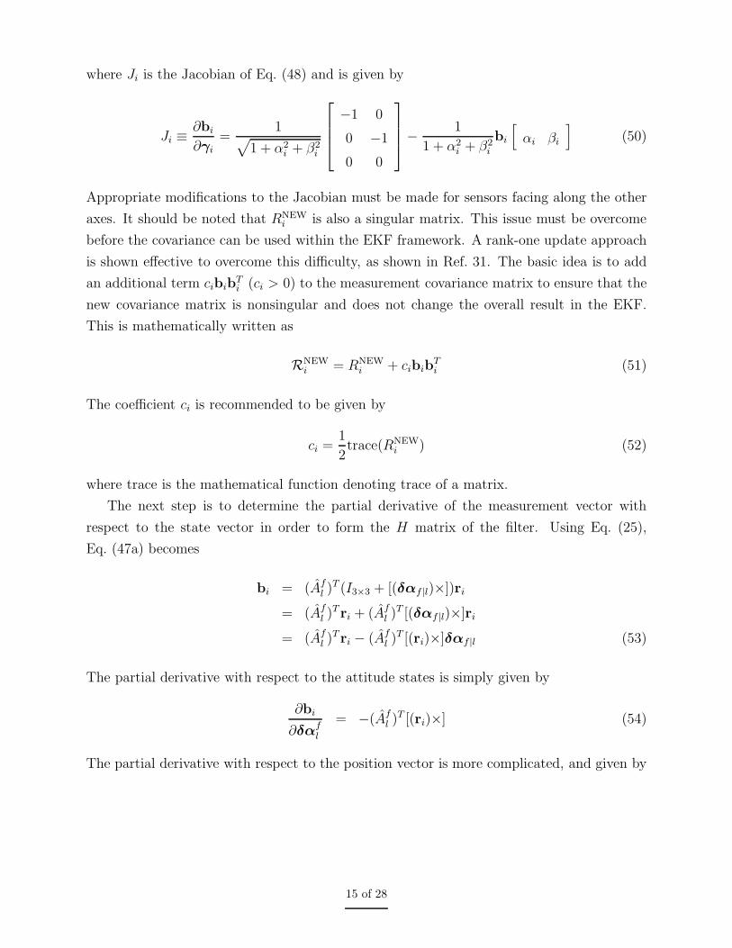
where Ji is the Jacobian of Eq. (48) and is given by
Ji ≡∂bi
∂γi
=1
√
1 + α2i + β2
i
−1 0
0 −1
0 0
−1
1 + α2i + β2
i
bi
[
αi βi
]
(50)
Appropriate modifications to the Jacobian must be made for sensors facing along the other
axes. It should be noted that RNEWi is also a singular matrix. This issue must be overcome
before the covariance can be used within the EKF framework. A rank-one update approach
is shown effective to overcome this difficulty, as shown in Ref. 31. The basic idea is to add
an additional term cibibTi (ci > 0) to the measurement covariance matrix to ensure that the
new covariance matrix is nonsingular and does not change the overall result in the EKF.
This is mathematically written as
RNEWi = RNEW
i + cibibTi (51)
The coefficient ci is recommended to be given by
ci =1
2trace(RNEW
i ) (52)
where trace is the mathematical function denoting trace of a matrix.
The next step is to determine the partial derivative of the measurement vector with
respect to the state vector in order to form the H matrix of the filter. Using Eq. (25),
Eq. (47a) becomes
bi = (Afl )
T (I3×3 + [(δαf |l)×])ri
= (Afl )
T ri + (Afl )
T [(δαf |l)×]ri
= (Afl )
T ri − (Afl )
T [(ri)×]δαf |l (53)
The partial derivative with respect to the attitude states is simply given by
∂bi
∂δαfl
= −(Afl )
T [(ri)×] (54)
The partial derivative with respect to the position vector is more complicated, and given by
15 of 28
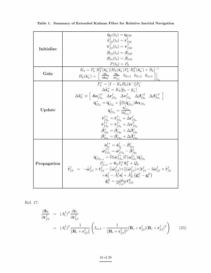
Table 1. Summary of Extended Kalman Filter for Relative Inertial Navigation
Initialize
qfl(t0) = qf |l0
rf
f |l(t0) = rf
f |l0
vf
f |l(t0) = vf
f |l0
βfg(t0) = βfg0
βfa(t0) = βfa0
P (t0) = P0
GainKk = P−
k HTk (x−
k )[Hk(x−k )P−
k HTk (x−
k ) + Rk]−1
Hk(x−k ) =
[
∂bi
∂δαfl
∂bi
∂rff |l
03×3 03×3 03×3
]∣
∣
∣
tk
Update
P+k = [I − KkHk(x
−)]P−k
∆ˆx+k = Kk[yk − y−
k ]
∆ˆx+k ≡
[
δα+Tf |lk
∆rf
f |lk∆v
f
f |lk∆β+T
fgk∆β+T
fak
]
q+f |lk
= q−f |lk
+ 12Ξ(q−
f |lk)δαf |lk
q+f |lk
=q
+
f |lk
‖q+
f |lk‖
rf+f |lk
= rf−f |lk
+ ∆rf
f |lk
vf+f |lk
= vf−f |lk
+ ∆vf
f |lk
β+fgk
= β−fgk
+ ∆β+fgk
β+fak
= β−fak
+ ∆β+fak
Propagation
af+fk
= affk− β+
fak
ωf+f |Ik
= ωf
f |Ik− β+
fgk
q−f |lk+1
= Ω(ωf+f |Ik
)Γ(ωl+l|Ik
)q+f |lk
P−k+1 = ΦkP
+k ΦT
k + Qk
¨rf
f |l = − ˙ωf
f |I × rf
f |l − [(ωf
f |I)×][(ωf
f |I)×]rf
f |l − 2ωf
f |I ×˙rf
f |l
+aff − Af
l all + Af
E
(
gEf − gE
l
)
gEf = −µ
‖rEf |E
‖3 rEf |E
Ref. 17:
∂bi
∂rf
f |l
= (Afl )
T ∂ri
∂rf
f |l
= (Afl )
T 1
‖Ri + rf
f |l‖
(
I3×3 −1
‖Ri + rf
f |l‖2(Ri + r
f
f |l)(Ri + rf
f |l)T
)
(55)
16 of 28
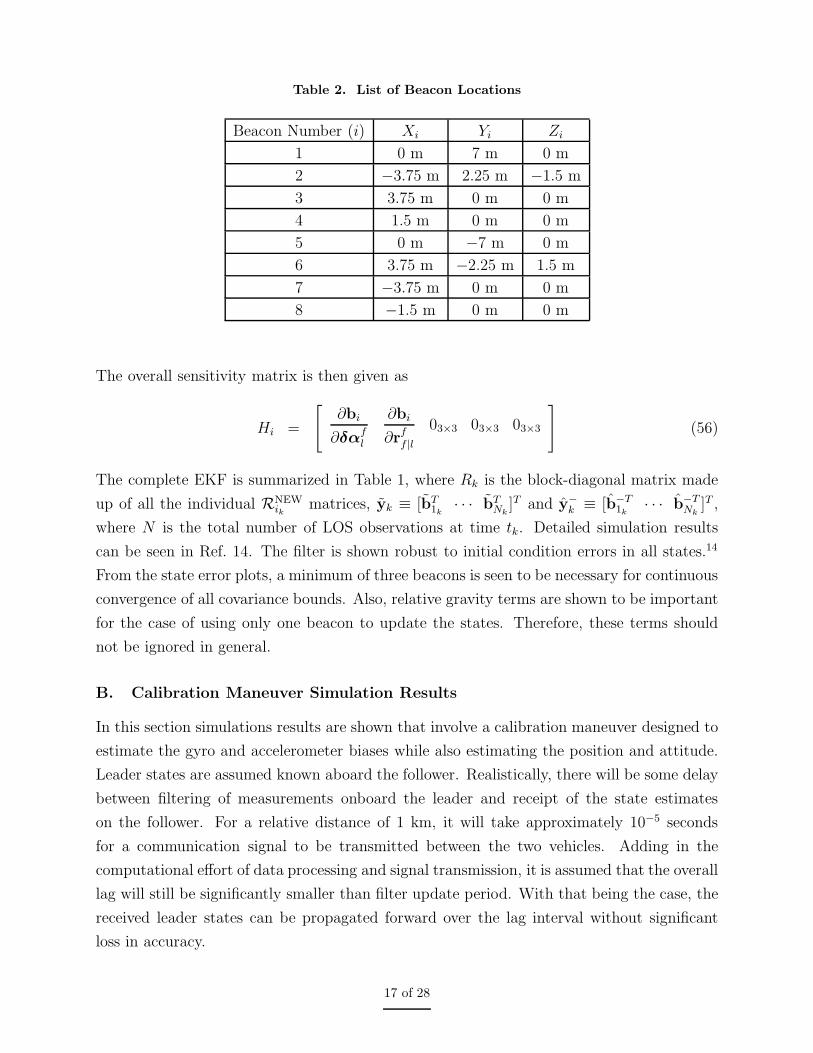
Table 2. List of Beacon Locations
Beacon Number (i) Xi Yi Zi
1 0 m 7 m 0 m
2 −3.75 m 2.25 m −1.5 m
3 3.75 m 0 m 0 m
4 1.5 m 0 m 0 m
5 0 m −7 m 0 m
6 3.75 m −2.25 m 1.5 m
7 −3.75 m 0 m 0 m
8 −1.5 m 0 m 0 m
The overall sensitivity matrix is then given as
Hi =
[
∂bi
∂δαfl
∂bi
∂rf
f |l
03×3 03×3 03×3
]
(56)
The complete EKF is summarized in Table 1, where Rk is the block-diagonal matrix made
up of all the individual RNEWik
matrices, yk ≡ [bT1k
· · · bTNk
]T and y−k ≡ [b−T
1k· · · b−T
Nk]T ,
where N is the total number of LOS observations at time tk. Detailed simulation results
can be seen in Ref. 14. The filter is shown robust to initial condition errors in all states.14
From the state error plots, a minimum of three beacons is seen to be necessary for continuous
convergence of all covariance bounds. Also, relative gravity terms are shown to be important
for the case of using only one beacon to update the states. Therefore, these terms should
not be ignored in general.
B. Calibration Maneuver Simulation Results
In this section simulations results are shown that involve a calibration maneuver designed to
estimate the gyro and accelerometer biases while also estimating the position and attitude.
Leader states are assumed known aboard the follower. Realistically, there will be some delay
between filtering of measurements onboard the leader and receipt of the state estimates
on the follower. For a relative distance of 1 km, it will take approximately 10−5 seconds
for a communication signal to be transmitted between the two vehicles. Adding in the
computational effort of data processing and signal transmission, it is assumed that the overall
lag will still be significantly smaller than filter update period. With that being the case, the
received leader states can be propagated forward over the lag interval without significant
loss in accuracy.
17 of 28
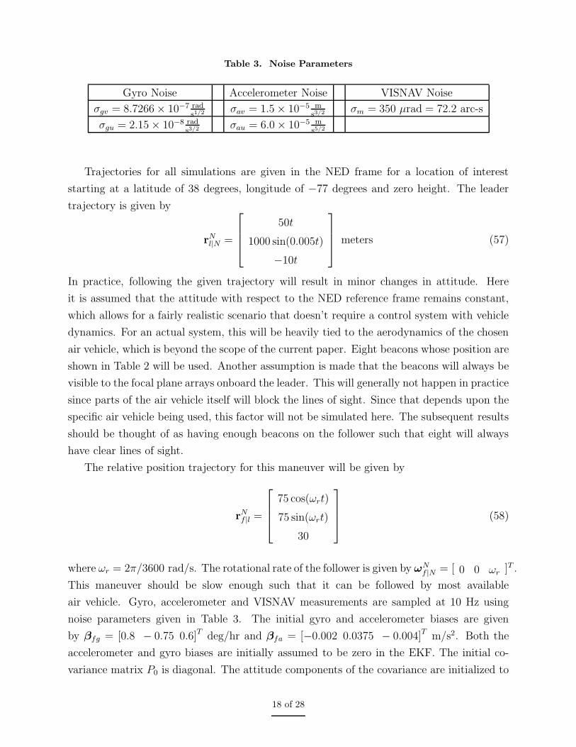
Table 3. Noise Parameters
Gyro Noise Accelerometer Noise VISNAV Noise
σgv = 8.7266 × 10⁻⁷ rads1/2 σav = 1.5 × 10⁻⁵ m
s3/2 σm = 350 µrad = 72.2 arc-s
σgu = 2.15 × 10⁻⁸ rads3/2 σau = 6.0 × 10⁻⁵ m
s5/2
Trajectories for all simulations are given in the NED frame for a location of interest
starting at a latitude of 38 degrees, longitude of −77 degrees and zero height. The leader
trajectory is given by
rNl|N =
50t
1000 sin(0.005t)
−10t
meters (57)
In practice, following the given trajectory will result in minor changes in attitude. Here
it is assumed that the attitude with respect to the NED reference frame remains constant,
which allows for a fairly realistic scenario that doesn’t require a control system with vehicle
dynamics. For an actual system, this will be heavily tied to the aerodynamics of the chosen
air vehicle, which is beyond the scope of the current paper. Eight beacons whose position are
shown in Table 2 will be used. Another assumption is made that the beacons will always be
visible to the focal plane arrays onboard the leader. This will generally not happen in practice
since parts of the air vehicle itself will block the lines of sight. Since that depends upon the
specific air vehicle being used, this factor will not be simulated here. The subsequent results
should be thought of as having enough beacons on the follower such that eight will always
have clear lines of sight.
The relative position trajectory for this maneuver will be given by
rNf |l =
75 cos(ωrt)
75 sin(ωrt)
30
(58)
where ωr = 2π/3600 rad/s. The rotational rate of the follower is given by ωNf |N = [ 0 0 ωr ]T .
This maneuver should be slow enough such that it can be followed by most available
air vehicle. Gyro, accelerometer and VISNAV measurements are sampled at 10 Hz using
noise parameters given in Table 3. The initial gyro and accelerometer biases are given
by βfg = [0.8 − 0.75 0.6]T deg/hr and βfa = [−0.002 0.0375 − 0.004]T m/s2. Both the
accelerometer and gyro biases are initially assumed to be zero in the EKF. The initial co-
variance matrix P0 is diagonal. The attitude components of the covariance are initialized to
18 of 28

0 100 200 300 400 500 600−10
0
10
0 100 200 300 400 500 600−10
0
10
0 100 200 300 400 500 600−10
0
10
Time (sec)
xy
z
(a) Position Errors ∆rf
f |l (cm)
0 100 200 300 400 500 600−50
0
50
0 100 200 300 400 500 600−50
0
50
0 100 200 300 400 500 600−50
0
50
Time (sec)
Roll
Pitch
Yaw
(b) Attitude Errors δαf |l (arc-s)
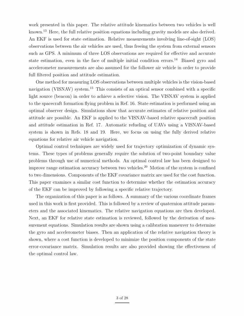
Figure 3. Relative Position and Attitude Errors
0 100 200 300 400 500 600−10
0
10
0 100 200 300 400 500 600−10
0
10
0 100 200 300 400 500 600−10
0
10
Time (sec)
xy
z
(a) Accelerometer Bias Errors (mm/s2)
0 100 200 300 400 500 600−1
0
1
0 100 200 300 400 500 600−1
0
1
0 100 200 300 400 500 600−1
0
1
Time (sec)
xy
z
(b) Gyro Bias Errors (deg/hr)
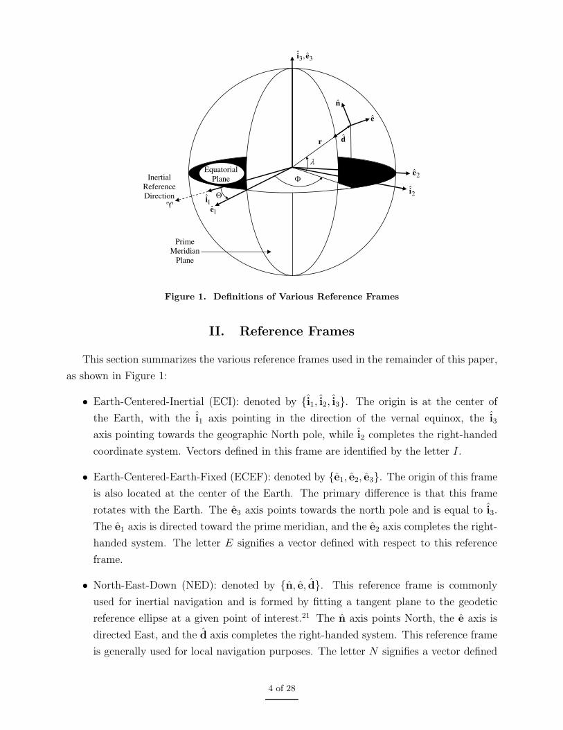
Figure 4. Bias Errors
a 3σ bound of 5 deg. The position and velocity parts have 3σ bounds of 20 m and 0.5 m/s,
respectively. The accelerometer and gyro bias components have 3σ bounds 1 deg/hr and 0.1
m/s2, respectively.
Figures 3 and 4 show the estimation errors for the calibration maneuver. All plots show
the average of errors over 100 Monte Carlo runs. Estimates of all states can be seen to
converge within their respective theoretical covariance bounds. Position errors are contained
within 3σ bounds of 10 cm, while the attitude errors are contained within 3σ bounds of
50 arc-seconds. All bias estimates are shown to converge quickly. These results clearly
show that the derived relative equations provide a viable means to accurately estimate both
relative attitude and position.
19 of 28
VI. Path Trajectory Application
In this section an application of the previously derived filter equations is shown. Specif-
ically, an optimal trajectory is designed to increase the observability of the relative position
states with control applied to the follower. In practical applications, this type of maneuver
would be applied between vehicle take-off and the arrival of the vehicles in their designated
mission area. The purpose is to achieve the best possible relative position information before
the mission begins. This task is assumed to be equivalent to improving the accuracy of the
position estimates of the EKF developed in the prior sections. Optimal control techniques
will be employed to design an optimal trajectory. It is assumed that this optimal path won’t
be used until after the primary state estimator has converged. This allows the bias states
to be ignored for this development. Two types of control are possible, rotational control
and translational control. In practical applications, the attitude of an air vehicle will be
constrained by the desired direction of motion and the aerodynamics that govern its flight.
For this reason, translational control will be the focus here. To keep this work from being
tied to any specific air vehicle, only a generic translational control term will be used. For
future applications, the following development will need to be repeated with the chosen air
vehicle’s dynamics to ensure that the resulting trajectory is feasible.
The measure of an EKF’s accuracy is defined by the 3σ bounds as given by the filter
covariance matrix. The cost function will look to minimize the diagonal elements of the
this matrix that correspond to the position states. In formulating the cost function, the
information form of the covariance update will be used:32
(P+k )−1 = (P−
k )−1 + HTk RkHk (59)
The previously derived filter used a sequential update, allowing the above equation to be
rewritten as
(P+k )−1 = (P−
k )−1 +
n∑
i=1
(
HTkiRkHki
)
(60)
≡ (P−k )−1 +
n∑
i=1
Bki (61)
The subscript i corresponds to the beacon number of the current Measurement, and n is the
total number of beacons.
Minimizing the desired elements of the updated covariance P+k requires maximizing its
inverse, and thus maximizing the right hand side of Eq. (59). Since the propagated covariance
P−k is given at each time step, maximizing the right hand side requires maximizing the
20 of 28
summation of Bki.20 Using Eq. (56) and the QUEST covariance to simplify the control design
only (the navigation equations still used the generalized covariance model), the submatrix
corresponding to the position elements is written as
Bki(4, 4) Bki(4, 5) Bki(4, 6)
Bki(5, 4) Bki(5, 5) Bki(5, 6)
Bki(6, 4) Bki(6, 5) Bki(6, 6)
=
(
∂bi
∂rf
f |l
)T
i
(
σ2I3×3
)
(
∂bi
∂rf
f |l
)
i
= σ2
(
∂bi
∂rf
f |l
)T
i
(
∂bi
∂rf
f |l
)
i
(62)
with the diagonal elements of this matrix given by
Bki(4, 4) =σ2 [(Yi + y)2 + (Zi + z)2]
(Ri + rf
f |l)T (Ri + r
f
f |l)(63a)
Bki(5, 5) =σ2 [(Xi + x)2 + (Zi + z)2]
(Ri + rf
f |l)T (Ri + r
f
f |l)(63b)
Bki(6, 6) =σ2 [(Xi + x)2 + (Yi + y)2]
(Ri + rf
f |l)T (Ri + r
f
f |l)(63c)
Optimal control problems are generally stated in terms of minimizing a function. Therefore,
maximizing∑n
i=1
∑6j=4 Bki(j, j) is accomplished by minimizing (−1)
∑n
i=1
∑6j=4 Bki(j, j),
which is written as
−3∑
i=1
6∑
j=4
Bki(j, j) = −3∑
i=1
2σ2
(Ri + rf
f |l)T (Ri + r
f
f |l)(64)
A numerical problem can be seen by examining the denominator. Minimizing Eq. (64)
requires the denominator to be made as small as possible. Its composition allows for it
to achieve a zero value, which results in a numerical singularity. To avoid this difficulty
a slightly different form of Eq. (64) will be used, given by w1
∑ni=1(Ri + r
f
f |l)T (Ri + r
f
f |l).
This removes the mathematical singularity while still resulting in the same minimum. The
constant coefficients have been replaced with a user specified weighting coefficient, w1.
Another difficulty with this term is that its minimum requires the follower to be driven
close to the leader. More specifically, the follower will asymptotically approach
(
rf
f |l
)
∗=
−1
n
n∑
i=1
Ri ≡−1
nRT (65)
Physically, this means that the follower will asymptotically approach a relative position such
21 of 28
that the mean beacon vector position will be located at the origin of the leader reference
frame. In practical applications, this will likely cause a collision between the vehicles. To
prevent such an occurrence, a state constraint will be imposed upon the system of the form
‖rf
f |l‖ ≥ rmin (66)
where rmin is the minimum desired distance between the origins of the two vehicles body
frames. For this constraint, it is assumed that the origins of the body frames are located
at the geometric center of each vehicle. If this is not the case, the constraint needs to be
modified appropriately.
The constraint can be appended into the loss function using a standard Lagrange multi-
plier approach.33 However, a numerical solution to this optimization problem may be difficult
to achieve. Here, a simpler method is used to impose the constraint, where an exponential
is appended to the cost function, which now has the form of
J [x(t),u(t)] =
∫ tf
t0
1
2w1
n∑
i=1
(Ri + rf
f |l(t))T (Ri + r
f
f |l(t)) +1
2w2
(
rf
f |l(t))T
rf
f |l(t)
+1
2w3
(
rf
f |l(t))T
rf
f |l(t) + w4 exp(
k(rmin − ‖rf
f |l(t)‖))
dt (67)
where k is a user-specified coefficient and u ≡ aff = Af
IaIf is contained within the relative
acceleration term. The primary goal of the follower during this calibration period is to
perform the same maneuver as the leader. Since improving the observability is a secondary
goal, the optimal trajectory should minimize deviations from that maneuver. This is why
the relative velocity and relative acceleration are used instead of the follower velocity and
follower acceleration.
The optimal control trajectory can be determined using standard unconstrained opti-
mization methods, but choosing w1 and w4 independently may violate the constraint. The
relation of the weight w4 to w1 is now shown. Equation (65) gives the minimum for an un-
constrained system. Now, consider a constraint sphere of radius rmin about the leader upon
which the follower is required to move. Because the cost function is based on the distance
from the beacons to the leader, the cost function will vary over the constraint sphere as
long as RT is non-zero. If this value is zero, the optimal trajectory will simply be a straight
line from the initial relative position to the closest point on the constraint sphere with the
speed and acceleration determined by the relative weights. The optimal relative position
will be that which forces RT to be normal to the constraint sphere and pointing inward.
22 of 28
Mathematically, this is written as
(rf
f |l)∗ = −rmin
RT
‖RT‖(68)
Since this value is constant, the optimal relative velocity and acceleration are given by
(rf
f |l)∗ = 0 (69a)
(rf
f |l)∗ = 0 (69b)
Knowing the desired location of the optimal position allows w4 to be determined as a function
of w1. The optimal position occurs when ∂J∂x
= 0. Since the optimal relative velocity and
relative acceleration are equal to zero, they aren’t present in the following development.
Working from Eq. (72), this partial derivative is given by
∂J
∂x= w1
n∑
i=1
(Ri + rf
f |l)T − kw4 exp
(
k(rmin − ‖rf
f |l‖)) (rf
f |l)T
‖rf
f |l‖
= w1(RT + nrf
f |l)T − kw4 exp
(
k(rmin − ‖rf
f |l‖)) (rf
f |l)T
‖rf
f |l‖
= w1(‖RT‖ − n rmin)(RT )T
‖RT‖+ kw4 exp (k(rmin − rmin))
(RT )T
‖RT‖= 0T
(70)
where the second line makes use of Eq. (68). Since the equation is solely a function of vectors
along the direction of RT , the magnitudes alone are used to solve the equation for w4. This
yields
w4 =w1
k(n rmin − ‖RT‖) (71)
Use of this equation allows an optimization to be performed without the use of Lagrange
multipliers to satisfy the inequality constraint. Equation (67) can then be written as
J [x(t),u(t)] =
∫ tf
t0
1
2w1
n∑
i=1
(Ri + rf
f |l(t))T (Ri + r
f
f |l(t))
+1
2w2
(
rf
f |l(t))T
rf
f |l(t) +1
2w3
(
rf
f |l(t))T
rf
f |l(t)
+w1
k(n rmin − ‖RT‖) exp
(
k(rmin − ‖rf
f |l(t)‖))
dt (72)
Even though the optimal position is known, it is still necessary to develop the trajectories that
23 of 28

will maneuver the follower from its initial location to that position. Trajectories developed
from this cost function will fall into one of two categories, which depend upon the location
of the follower with respect to the constraint sphere and the constrained optimal position. If
a direct path would require movement through the constraint sphere, the resulting optimal
trajectory will drive the follower onto that sphere, and then follow a path along the sphere
to the optimal position. Otherwise, the path will only be constrained by the user-specified
weighting coefficients.
A. Simulation Results
This section shows simulation results of a maneuver using the previously developed optimal
control law, along with several other trajectories to provide points of comparison. Three
beacons have been determined to be the minimum required for continuous observability by
simulations performed in Ref. 34. The first three beacons of Table 2 will therefore be used to
generate the optimal trajectory. Once again, the number of beacons onboard the air vehicle
will generally need to be higher to ensure that this minimum number always has clear lines
of sight. For practical applications, a geometric analysis of the host vehicle structure, the
possible locations of its beacons and the possible relative positions of the communicating
vehicles will be required.
The other relevant parameters in developing the trajectory are a minimum distance of
rmin = 20 meters and weights of w1 = 100, w2 = 1 and w3 = 40. The value of rmin is
chosen so that it would prevent collisions of larger air vehicles, such as the Predator which
has a wingspan of approximately fifteen meters. When computing an optimal trajectory for
smaller air vehicles, this constraint should be reduced appropriately. Weights for the cost
function are chosen by balancing the desire for a quick approach to the optimal position
with the need to prevent control inputs from becoming unrealistic. The above weights yield
a trajectory that reasonably satisfies these competing factors.
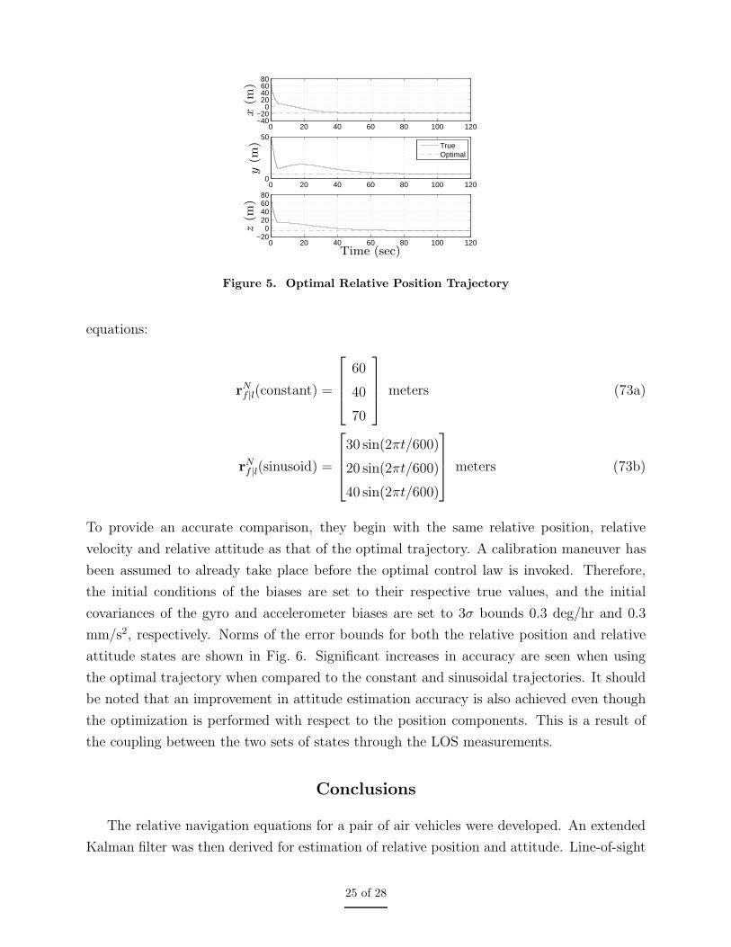
Figure 5 shows the resulting optimal trajectory in NED coordinates. Each subplot shows
two lines. The solid line corresponds to the computed true trajectory, while the dashed line
corresponds to the optimal position. Initially, all three position components move towards
their respective optimal positions. After about five seconds, the y component then begins
to increase. This is due to the fact that both the x and z components have to cross zero
in order to reach their optimal positions. In order for the minimum distance constraint
to be maintained, the y position must increase. It is this type of feature that requires an
optimal trajectory to be calculated. If the follower just traveled straight towards the optimal
position, there is a chance that the constraint will be violated resulting in a possible collision.
Two additional trajectories are tested for comparison. They are given by the following
24 of 28
0 20 40 60 80 100 120−40−20
020406080
0 20 40 60 80 100 1200
50
0 20 40 60 80 100 120−20
020406080
TrueOptimal
Time (sec)x
(m)
y(m
)z
(m)
Figure 5. Optimal Relative Position Trajectory
equations:
rNf |l(constant) =
60
40
70
meters (73a)
rNf |l(sinusoid) =
30 sin(2πt/600)
20 sin(2πt/600)
40 sin(2πt/600)
meters (73b)
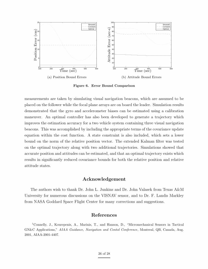
To provide an accurate comparison, they begin with the same relative position, relative
velocity and relative attitude as that of the optimal trajectory. A calibration maneuver has
been assumed to already take place before the optimal control law is invoked. Therefore,
the initial conditions of the biases are set to their respective true values, and the initial
covariances of the gyro and accelerometer biases are set to 3σ bounds 0.3 deg/hr and 0.3
mm/s2, respectively. Norms of the error bounds for both the relative position and relative
attitude states are shown in Fig. 6. Significant increases in accuracy are seen when using
the optimal trajectory when compared to the constant and sinusoidal trajectories. It should
be noted that an improvement in attitude estimation accuracy is also achieved even though
the optimization is performed with respect to the position components. This is a result of
the coupling between the two sets of states through the LOS measurements.
Conclusions
The relative navigation equations for a pair of air vehicles were developed. An extended
Kalman filter was then derived for estimation of relative position and attitude. Line-of-sight
25 of 28
100 200 300 400 500 6000
5
10
15
20
25
SinusoidConstantOptimal
Time (sec)
Posi
tion
Err
or
(cm
)
(a) Position Bound Errors
100 200 300 400 500 6000
10
20
30
40
50
60
70
80
90
100
SinusoidConstantOptimal
Time (sec)
Att
itude
Err
or
(arc
-s)
(b) Attitude Bound Errors
Figure 6. Error Bound Comparison
measurements are taken by simulating visual navigation beacons, which are assumed to be
placed on the follower while the focal plane arrays are on board the leader. Simulation results
demonstrated that the gyro and accelerometer biases can be estimated using a calibration
maneuver. An optimal controller has also been developed to generate a trajectory which
improves the estimation accuracy for a two vehicle system containing three visual navigation
beacons. This was accomplished by including the appropriate terms of the covariance update
equation within the cost function. A state constraint is also included, which sets a lower
bound on the norm of the relative position vector. The extended Kalman filter was tested
on the optimal trajectory along with two additional trajectories. Simulations showed that
accurate position and attitudes can be estimated, and that an optimal trajectory exists which
results in significantly reduced covariance bounds for both the relative position and relative
attitude states.
Acknowledgement
The authors wish to thank Dr. John L. Junkins and Dr. John Valasek from Texas A&M
University for numerous discussions on the VISNAV sensor, and to Dr. F. Landis Markley
from NASA Goddard Space Flight Center for many corrections and suggestions.
References
1Connelly, J., Kourepenis, A., Marinis, T., and Hanson, D., “Micromechanical Sensors in Tactical
GN&C Applications,” AIAA Guidance, Navigation and Contol Conference, Montreal, QB, Canada, Aug.
2001, AIAA-2001-4407.
26 of 28

2MacSween-George, S. L., “Will the Public Accept UAVs for Cargo and Passenger Transportation?”
Proceedings of the IEEE Aerospace Conference, Vol. 1, IEEE Publications, Piscataway, NJ, 2003, pp. 357–
367.
3Sarris, Z., “Survey of UAV Applications in Civil Markets,” The 9th Mediterranean Conference on
Control and Automation, Dubrovnik, Croatia, June 2001, ISBN 953-6037-35-1, MED01-164.
4DeGarmo, M. and Nelson, G., “Prospective Unmanned Aerial Vehicle Operations in the Future
National Airspace System,” AIAA 4th Aviation Technology, Integration and Operations (ATIO) Forum,
Chicago, IL, Sept. 2004, AIAA-2004-6243.
5Ryan, A., Zennaro, M., Howell, A., Sengupta, R., and Hedrick, J. K., “An Overview of Emerging
Results in Cooperative UAV Control,” Proceedings of the 43th IEEE Conference on Decision and Control ,
Vol. 1, IEEE Publications, Piscataway, NJ, 2004, pp. 602–607.
6Johnson, E. N., Calise, A. J., Sattigeri, R., Watanabe, Y., and Madyastha, V., “Approaches to Vision-
Based Formation Control,” Proceedings of the 43th IEEE Conference on Decision and Control , Vol. 2, IEEE
Publications, Piscataway, NJ, Dec. 2004, pp. 1643–1648.
7Aidala, V. J. and Hammel, S. E., “Utilization of Modified Polar Coordinates for Bearings-Only Track-
ing,” IEEE Transactions on Automatic Control , Vol. 28, No. 3, March 1983, pp. 283–294.
8Chatfield, A. B., Fundamentals of High Accuracy Inertial Navigation, chap. 9, American Institute of
Aeronautics and Astronautics, Inc., Reston, VA, 1997.
9Crassidis, J. L., “Sigma-Point Kalman Filtering for Integrated GPS and Inertial Navigation,” IEEE
Transactions on Aerospace and Electronic Systems , Vol. 42, No. 2, April 2006, pp. 750–756.
10Gustafsson, F., Gunnarsson, F., Bergman, N., Forssell, U., Jansson, J., Karlsson, R., and Nordlund,
P.-J., “Particle Filters for Positioning, Navigation, and Tracking,” IEEE Transactions on Signal Processing,
Vol. 50, No. 2, Feb. 2002, pp. 425–435.
11Felter, S. C. and Wu, N. E., “A Relative Navigation System for Formation Flight,” IEEE Transactions
on Aerospace and Electronic Systems , Vol. 33, No. 3, July 1997, pp. 958–967.
12Woo, M. J. and Choi, J. W., “A Relative Navigation System for Vehicle Platooning,” Proceedings of
the 40th SICE Annual Conference, IEEE Publications, Piscataway, NJ, July 2001, pp. 28–31.
13Mayo, R. A., “Relative Quaternion State Transition Relation,” Journal of Guidance, Navigation and
Control , Vol. 2, No. 1, Jan-Feb. 1979, pp. 44–48.
14Fosbury, A. M. and Crassidis, J. L., “Kalman Filtering for Relative Inertial Navigation of Uninhabited
Air Vehicles,” AIAA Guidance, Navigation, and Control Conference, Keystone, CO, Aug. 2006, AIAA-2006-
6544.
15Junkins, J. L., Hughes, D. C., Wazni, K. P., and Pariyapong, V., “Vision-Based Navigation for Ren-
dezvous, Docking and Proximity Operations,” 22nd Annual AAS Guidance and Control Conference, Breck-
enridge, CO, Feb. 1999, AAS-99-021.
16Alonso, R., Crassidis, J. L., and Junkins, J. L., “Vision-Based Relative Navigation for Formation Flying
of Spacecraft,” AIAA Guidance, Navigation, and Control Conference, Denver, CO, Aug. 2000, AIAA-00-
4439.
17Kim, S. G., Crassidis, J. L., Cheng, Y., Fosbury, A. M., and Junkins, J. L., “Kalman Filtering
for Relative Spacecraft Attitude and Position Estimation,” Journal of Guidance, Control, and Dynamics,
Vol. 30, No. 1, Jan.-Feb. 2007, pp. 133–143.
27 of 28
18Valasek, J., Gunnam, K., Kimmett, J., Junkins, J. L., Hughes, D., and Tandale, M. D., “Vision-
Based Sensor and Navigation System for Autonomous Air Refueling,” Journal of Guidance, Control, and
Dynamics , Vol. 28, No. 5, Sept.-Oct. 2005, pp. 979–989.
19Tandale, M. D., Bowers, R., and Valasek, J., “Robust Trajectory Tracking Controller for Vision Based
Autonomous Aerial Refueling of Unmanned Aircraft,” Journal of Guidance, Control, and Dynamics, Vol. 29,
No. 4, July-Aug. 2006, pp. 846–857.
20Watanabe, Y., Johnson, E. N., and Calise, A. J., “Optimal 3-D Guidance from a 2-D Vision Sensor,”
AIAA Guidance, Navigation and Control Conference, Providence, RI, Aug. 2004, AIAA-2004-4779.
21Farrell, J. and Barth, M., The Global Positioning System and Inertial Navigation, chap. 2, McGraw-
Hill, New York, NY, 1998.
22Shuster, M. D., “A Survey of Attitude Representations,” Journal of the Astronautical Sciences , Vol. 41,
No. 4, Oct.-Dec. 1993, pp. 439–517.
23Schaub, H. and Junkins, J. L., Analytical Mechanics of Aerospace Systems, American Institute of
Aeronautics and Astronautics, Inc., New York, NY, 2003, pp. 72–78.
24Lefferts, E. J., Markley, F. L., and Shuster, M. D., “Kalman Filtering for Spacecraft Attitude Estma-
tion,” Journal of Guidance, Control, and Dynamics, Vol. 5, No. 5, Sept.-Oct. 1982, pp. 417–429.
25Crassidis, J. L., “Sigma-Point Kalman Filtering for Integrated GPS and Inertial Navigation,” AIAA
Guidance, Navigation, and Control Conference, San Francisco, CA, Aug. 2005, AIAA-05-6052.
26Fosbury, A. M., Control of Relative Attitude Dynamics of a Formation Flight Using Model-Error
Control Synthesis , Master’s thesis, University at Buffalo, State University of New York, March 2005.
27Van-Loan, C. F., “Computing Integrals Involving Matrix Exponentials,” IEEE Transactions on Auto-
matic Control , Vol. AC-23, No. 3, Jun. 1978, pp. 396–404.
28Light, D. L., “Satellite Photogtammetry,” Maunual of Photogrammetry, edited by C. C. Slama, chap.
17, American Society of Photogrammetry, Falls Church, VA, 4th ed., 1980.
29Shuster, M. D., “Kalman Filtering of Spacecraft Attitude and the QUEST Model,” Journal of the
Astronautical Sciences , Vol. 38, No. 3, July-Sept. 1990, pp. 377–393.
30Shuster, M. D. and Oh, S. D., “Three Axis Attitude Determination from Vector Observations,” Journal
of Guidance, Navigation and Control , Vol. 4, No. 1, Jan-Feb. 1981, pp. 70–77.
31Cheng, Y., Crassidis, J. L., and Markley, F. L., “Attitude Estimation for Large Field-of-View Sensors,”
Journal of the Astronautical Sciences , Vol. 54, No. 3-4, July-Dec. 2006, pp. 433–448.
32Crassidis, J. L. and Junkins, J. L., Optimal Estimation of Dynamic Systems, chap. 5, Chapman &
Hall/CRC, Boca Raton, FL, 2004.
33Bryson, A. E., Dynamic Optimization, chap. 9, Addison Wesley Longman, Menlo Park, CA, 1999.
34Fosbury, A., Control and Kalman Filtering for the Relative Dynamics of a Formation of Uninhabited
Autonomous Vehicles , Ph.D. thesis, University at Buffalo, State University of New York, August 2006.
28 of 28