Embed Size (px)
Citation preview

Relationships between variables
Statistics for the Social SciencesPsychology 340
Spring 2010

PSY 340Statistics for the
Social Sciences Exam 3 results
• Mean = 86.9• Median = 89.0• Great job!

PSY 340Statistics for the
Social Sciences Final project
• Details posted on website• Download the Harass.sav datafile (fictional dataset
of harassment within a workplace)• Conduct analyses to answer 8 different questions• Write up the results of you analyses
• Worth 15% of final grade

PSY 340Statistics for the
Social SciencesOutline (for 2 weeks)
• Correlation– Scatterplot, hypothesis testing, computations, SPSS
• Simple bi-variate regression, least-squares fit line– The general linear model
– Residual plots
– Using SPSS
• Multiple regression– Comparing models, Delta r2
– Using SPSS

PSY 340Statistics for the
Social Sciences Correlation
• Correlations describe relationships between two variables
– Age and coordination skills in children, as kids get older their motor coordination tends to improve
– Price and quality, generally the more expensive something is the higher in quality it is

PSY 340Statistics for the
Social Sciences Correlation
• Correlations describe relationships between two variables, but DO NOT explain why the variables are related
Suppose that Dr. Steward finds that rates of spilled coffee and severity of plane turbulents are strongly positively correlated.
One might argue that turbulents cause coffee spills
One might argue that spilling coffee causes turbulents

PSY 340Statistics for the
Social Sciences Correlation
• Correlations describe relationships between two variables, but DO NOT explain why the variables are related
Suppose that Dr. Cranium finds a positive correlation between head size and digit span (roughly the number of digits you can remember).
One might argue that bigger your head, the larger your digit span
1
21
24
1537
One might argue that head size and digit span both increase with age (but head size and digit span aren’t directly related)
PSY 340Statistics for the
Social Sciences Correlation
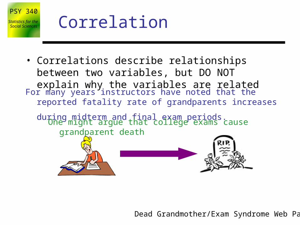
• Correlations describe relationships between two variables, but DO NOT explain why the variables are related
For many years instructors have noted that the reported fatality rate of
grandparents increases during midterm and final exam periods. One might argue that college exams cause grandparent death
Dead Grandmother/Exam Syndrome Web Page

PSY 340Statistics for the
Social Sciences Relationships between variables
• How variables co-vary with one another– As a descriptive statistic
• To examine this relationship you should:– Make a scatterplot - a picture of the relationship– Compute the Correlation Coefficient - a numerical description of the
relationship
• Properties of a correlation– Form (linear or non-linear)– Direction (positive or negative)– Strength (none, weak, strong, perfect)
– As an inferential statistic – comparing an observed correlation with a correlation expected due to chance

PSY 340Statistics for the
Social Sciences Scatterplot: Graphing Correlations
• Steps for making a scatterplot1. Draw axes and assign variables to
them
2. Determine range of values for each variable and mark on axes
3. Mark a dot for each person’s pair of scores
Hours
studied
Quiz
performance
A 6 6B 1 2C 5 6
D 3 4
E 3 2
X Y
Example: What is the relationship between how much you study and exam performance?

PSY 340Statistics for the
Social Sciences Scatterplot
Y
X1
2
34
5
6
1 2 3 4 5 6
• Plots one variable against the other• Each point
corresponds to a different individual
A 6 6
X Y
B 1 2C 5 6
D 3 4
E 3 2

PSY 340Statistics for the
Social Sciences Scatterplot
Y
X1
2
34
5
6
1 2 3 4 5 6
• Plots one variable against the other• Each point
corresponds to a different individual
A 6 6B 1 2
X Y
C 5 6
D 3 4
E 3 2

PSY 340Statistics for the
Social Sciences Scatterplot
Y
X1
2
34
5
6
1 2 3 4 5 6
• Plots one variable against the other• Each point
corresponds to a different individual
A 6 6B 1 2C 5 6
X Y
D 3 4
E 3 2

PSY 340Statistics for the
Social Sciences Scatterplot
Y
X1
2
34
5
6
1 2 3 4 5 6
• Plots one variable against the other• Each point
corresponds to a different individual
A 6 6B 1 2C 5 6
D 3 4
X Y
E 3 2

PSY 340Statistics for the
Social Sciences Scatterplot
Y
X1
2
34
5
6
1 2 3 4 5 6
• Plots one variable against the other• Each point
corresponds to a different individual
A 6 6B 1 2C 5 6
D 3 4
E 3 2
X Y

PSY 340Statistics for the
Social Sciences Scatterplot
Y
X1
2
34
5
6
1 2 3 4 5 6
• Imagine a line through the data points
• Plots one variable against the other• Each point
corresponds to a different individual
A 6 6B 1 2C 5 6
D 3 4
E 3 2
X Y
• Useful for “seeing” the relationship– Form, Direction,
and Strength

PSY 340Statistics for the
Social Sciences Form
Non-linearLinear

PSY 340Statistics for the
Social Sciences
NegativePositive
Direction
• X & Y vary in the same direction
• As X goes up, Y goes up
• Positive Pearson’s r
• X & Y vary in opposite directions
• As X goes up, Y goes down
• Negative Pearson’s r
Y
X
Y
X

PSY 340Statistics for the
Social Sciences Strength
• The strength of the relationship– Spread around the line (note the axis scales)
– Correlation coefficient will range from -1 to +1• Zero means “no relationship”
• The farther the r is from zero, the stronger the relationship

PSY 340Statistics for the
Social Sciences Strength
r = 1.0“perfect positive corr.”r2 = 100%
r = -1.0“perfect negative corr.”r2 = 100%
r = 0.0“no relationship”r2 = 0.0
-1.0 0.0 +1.0
The farther from zero, the stronger the relationship

PSY 340Statistics for the
Social Sciences Hypothesis testing with Pearson’s r
• Hypothesis testing– Core logic of hypothesis testing
• Considers the probability that the result of a study could have come about if the experimental procedure had no effect
• If this probability is low, scenario of no effect is rejected and the theory behind the experimental procedure is supported
• Step 1: State your hypotheses
• Step 2: Set your decision criteria
• Step 3: Collect your data
• Step 4: Compute your test statistics
• Step 5: Make a decision about your null hypothesis
– A five step program

PSY 340Statistics for the
Social Sciences
– Step 1: State your hypotheses: as a research hypothesis and a null hypothesis about the populations
• Null hypothesis (H0)
• Research hypothesis (HA)
Hypothesis testing with Pearson’s r
• There are no correlation between the variables (they are independent)
• Generally, the variables correlated (they are not independent)

PSY 340Statistics for the
Social Sciences Hypothesis testing with Pearson’s r
r ≥
r <
H0:
HA:
– Our theory is that the variables are negatively correlated
– Step 1: State your hypotheses
One -tailed
Note: sometimes the
symbol ρ (rho) is used
Note: sometimes the
symbol ρ (rho) is used

PSY 340Statistics for the
Social Sciences Hypothesis testing with Pearson’s r
r > 0
r < 0
H0:
HA:
– Our theory is that the variables are negatively correlated
– Step 1: State your hypotheses
One -tailed
r = 0
r ≠ 0
H0:
HA:
– Our theory is that the variables are correlated
Two -tailed

PSY 340Statistics for the
Social Sciences Hypothesis testing with Pearson’s r
– Step 2: Set your decision criteria• Your alpha (α) level will be your guide for when to reject or fail
to reject the null hypothesis. – Based on the probability of making making an certain type of
error

PSY 340Statistics for the
Social Sciences Hypothesis testing with Pearson’s r
– Step 3: Collect your data• Descriptive statistics (Pearson’s r)
6 61 25 6
3 4
3 2
X Y
• Common formulas for the correlation coefficient:
€
r =SP
SSX SSY
€
SP = X − X ( ) Y −Y ( )∑
Used this one in PSY138
r = XZ YZ∑N
Z-score alternative
For an example of the z-score alternative, skip to the end of the powerpoint
PSY 340Statistics for the
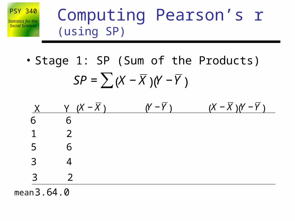
Social Sciences Computing Pearson’s r (using SP)
• Stage 1: SP (Sum of the Products)
€
SP = X − X ( ) Y −Y ( )∑
mean 3.6 4.0
6 61 25 6
3 4
3 2
X Y
€
X − X ( )
€
Y −Y ( )
€
X − X ( ) Y −Y ( )

PSY 340Statistics for the
Social Sciences Computing Pearson’s r (using SP)
• Stage 1: SP (Sum of the Products)
€
SP = X − X ( ) Y −Y ( )∑
mean 3.6 4.0
2.4
0.0
6 61 25 6
3 4
3 2
X Y
€
X − X ( )
€
Y −Y ( )
€
X − X ( ) Y −Y ( )= 6 - 3.6
-2.6 = 1 - 3.6
1.4 = 5 - 3.6
-0.6 = 3 - 3.6
-0.6 = 3 - 3.6
Quick check

PSY 340Statistics for the
Social Sciences Computing Pearson’s r (using SP)
• Stage 1: SP (Sum of the Products)
€
SP = X − X ( ) Y −Y ( )∑
mean 3.6 4.0
2.4-2.6
1.4
-0.6
-0.6
0.0 0.0
6 61 25 6
3 4
3 2
X Y
€
X − X ( )
€
Y −Y ( )
€
X − X ( ) Y −Y ( )2.0 = 6 - 4.0
-2.0 = 2 - 4.0
2.0 = 6 - 4.0
0.0= 4 - 4.0
-2.0= 2 - 4.0
Quick check

PSY 340Statistics for the
Social Sciences Computing Pearson’s r (using SP)
• Stage 1: SP (Sum of the Products)
€
SP = X − X ( ) Y −Y ( )∑
mean 3.6 4.0
2.4-2.6
1.4
-0.6
-0.6
0.0
2.0-2.0
2.0
0.0
-2.0
0.0 14.0 SP
6 61 25 6
3 4
3 2
X Y
€
X − X ( )
€
Y −Y ( )
€
X − X ( ) Y −Y ( )4.8* =
5.2* =
2.8* =
0.0* =
1.2* =

PSY 340Statistics for the
Social Sciences Computing Pearson’s r (using SP)
• Stage 2: SSX & SSY

PSY 340Statistics for the
Social Sciences Computing Pearson’s r (using SP)
• Stage 2: SSX & SSY
mean 3.6 4.0
2.4-2.6
1.4
-0.6
-0.6
0.0
2.0-2.0
2.0
0.0
-2.0
0.0 14.0
6 61 25 6
3 4
3 2
X Y
€
X − X ( )
€
Y −Y ( )
€
X − X ( ) Y −Y ( )4.85.2
2.8
0.0
1.2
€
X − X ( )2
5.76
15.20
SSX
2 =6.762 =
1.962 =
0.362 =
0.362 =

PSY 340Statistics for the
Social Sciences Computing Pearson’s r (using SP)
• Stage 2: SSX & SSY
mean 3.6 4.0
2.4-2.6
1.4
-0.6
-0.6
0.0
2.0-2.0
2.0
0.0
-2.0
0.0 14.0
6 61 25 6
3 4
3 2
X Y
€
X − X ( )
€
Y −Y ( )
€
X − X ( ) Y −Y ( )4.85.2
2.8
0.0
1.2
€
X − X ( )2
5.766.76
1.96
0.36
0.36
15.20
€
Y −Y ( )2
2 = 4.02 = 4.02 = 4.02 = 0.02 = 4.0
16.0
SSY

PSY 340Statistics for the
Social Sciences Computing Pearson’s r (using SP)
• Stage 3: compute r
€
r =SP
SSX SSY

PSY 340Statistics for the
Social Sciences Computing Pearson’s r (using SP)
• Stage 3: compute r
mean 3.6 4.0
2.4-2.6
1.4
-0.6
-0.6
0.0
2.0-2.0
2.0
0.0
-2.0
0.0 14.0
6 61 25 6
3 4
3 2
X Y
€
X − X ( )
€
Y −Y ( )
€
X − X ( ) Y −Y ( )4.85.2
2.8
0.0
1.2
€
X − X ( )2
5.766.76
1.96
0.36
0.36
15.20
€
Y −Y ( )2
4.04.0
4.0
0.0
4.0
16.0
SSYSSX
SP
€
r =SP
SSX SSY

PSY 340Statistics for the
Social Sciences Computing Pearson’s r
• Stage 3: compute r
14.015.20 16.0
SSYSSX
SP
€
r =SP
SSX SSY

PSY 340Statistics for the
Social Sciences Computing Pearson’s r
• Stage 3: compute r
15.20 16.0
SSYSSX
r =14
SSXSSY

PSY 340Statistics for the
Social Sciences Computing Pearson’s r
• Stage 3: compute r
15.20
SSX
r =14
SSX * 16

PSY 340Statistics for the
Social Sciences Computing Pearson’s r
• Stage 3: compute r
€
r =14
15.2 *16

PSY 340Statistics for the
Social Sciences Computing Pearson’s r
• Stage 3: compute r
r =14
15.2 * 16=.89
Y
X1
2
34
5
6
1 2 3 4 5 6
• Appears linear
• Positive relationship
• Fairly strong relationship• .89 is far from 0, near +1

PSY 340Statistics for the
Social Sciences Hypothesis testing with Pearson’s r
– Step 4: Compute your test statisticsr = 0.89 • Descriptive statistics (Pearson’s r)
• Inferential statistics: 2 choices (really the same):– A t-test & the t-table
– Use the Pearson’s r table (if available)
• Compute your degrees of freedom (df) df = n - 2 = 5 - 2 = 3

PSY 340Statistics for the
Social Sciences Hypothesis testing with Pearson’s r
– Step 4: Compute your test statistics• Descriptive statistics (Pearson’s r)
• Inferential statistics: 2 choices (really the same):– A t-test & the t-table
– Use the Pearson’s r table (if available)
t =r( ) n−2( )
1−r2=
.89( ) 3( )
1 − .79= 3.38
• From table, with df = n - 2 = 3: tcrit = 3.18
• Reject H0
• Conclude that the correlation is ≠0
– Step 5: Make a decision about your null hypothesis
r = 0.89

PSY 340Statistics for the
Social Sciences
Proportion in one tail 0.05 0.025 0.01 0.005
Proportion in two tails df 0.10 0.05 0.02 0.01 1 .988 .997 .9995 .9999 2 .900 .950 .980 .990 3 .805 .878 .934 .959 4 .729 .811 .882 .917 5 .669 .754 .833 .874 6 .622 .707 .789 .834 :
15 :
: .412
:
: .482
:
: .558
:
: .606
:
Hypothesis testing with Pearson’s r
– Step 4: Compute your test statistics
• From table– α-level = 0.05
– Two-tailed
– df = n - 2 = 3
– rcrit = 0.878
• Reject H0
• Conclude that the correlation is ≠0
– Step 5: Make a decision about your null hypothesis
• Descriptive statistics (Pearson’s r)
• Inferential statistics: 2 choices (really the same):– A t-test & the t-table
– Use the Pearson’s r table (if available)
r = 0.89

PSY 340Statistics for the
Social Sciences Effect sizes with Pearson’s r
• Pearson’s r is considered a measure of the effect size – Small r = 0.10
– Medium r = 0.30
– Large r = 0.50

PSY 340Statistics for the
Social SciencesA few more things to consider about correlation
• Correlations are greatly affected by the range of scores in the data– Consider height and age relationship
• Extreme scores can have dramatic effects on correlations – A single extreme score can radically change r
• When considering "how good" a relationship is, we really should consider r2 (coefficient of determination), not just r.

PSY 340Statistics for the
Social Sciences Correlation in SPSS
• Enter each variable in separate columns– Analyze -> Correlate -> bi-variate
– Enter all variables you want to examine• In options can request cross products and means
– Output – given as a matrix
– For the scatterplot: • Graphs -> legacy dialogs-> scatter/dot -> simple scatter
• Enter which is your X var. and which is your Y var.

PSY 340Statistics for the
Social Sciences Correlation in Research Articles
• Correlation matrix– A display of the correlations between more than two
variablesAcculturation
• Why have a “-”?
• Why only half the table filled with numbers?

PSY 340Statistics for the
Social Sciences Next time
• Regression: Predicting a variable based on other variables

PSY 340Statistics for the
Social Sciences The Correlation Coefficient
• Formulas for the correlation coefficient:
r = XZ YZ∑N
r =SP
SSXSSY
SP = X−X( ) Y −Y( )∑
Used this one in PSY138 Common alternative
PSY 340Statistics for the
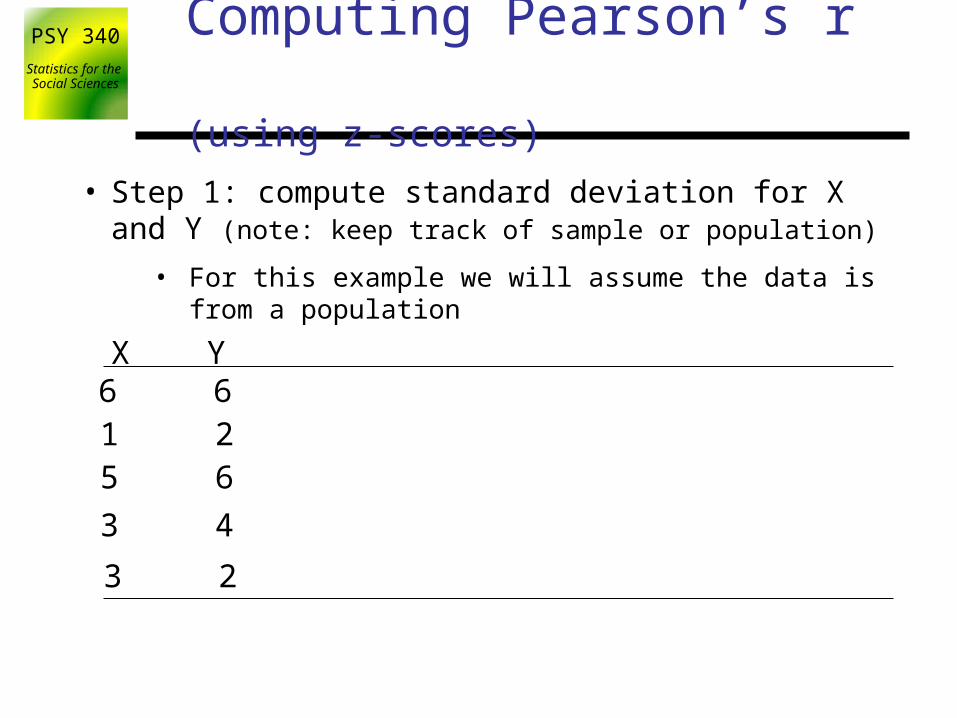
Social Sciences
Computing Pearson’s r (using z-scores)
• Step 1: compute standard deviation for X and Y (note: keep track of sample or population)
6 61 25 6
3 4
3 2
X Y
• For this example we will assume the data is from a population

PSY 340Statistics for the
Social Sciences
Computing Pearson’s r (using z-scores)
• Step 1: compute standard deviation for X and Y (note: keep track of sample or population)
Mean 3.6
2.4-2.6
1.4
-0.6
-0.6
0.0
6 61 25 6
3 4
3 2
X Y
€
X − X ( )
€
X − X ( )2
5.766.76
1.96
0.36
0.36
15.20
SSXStd dev 1.74
σ =SSX
N=
15.2
5= 1.74
• For this example we will assume the data is from a population

PSY 340Statistics for the
Social Sciences
Computing Pearson’s r (using z-scores)
• Step 1: compute standard deviation for X and Y (note: keep track of sample or population)
Mean 3.6 4.0
2.4-2.6
1.4
-0.6
-0.6
2.0-2.0
2.0
0.0
-2.0
0.0
6 61 25 6
3 4
3 2
X Y X −X( )
€
Y −Y ( )X −X( )2
5.766.76
1.96
0.36
0.36
15.20
€
Y −Y ( )2
4.04.0
4.0
0.0
4.0
16.0
SSYStd dev 1.74 1.79
• For this example we will assume the data is from a population
σ =SSY
N
=16.0
5= 1.79

PSY 340Statistics for the
Social Sciences
Computing Pearson’s r (using z-scores)
• Step 2: compute z-scores
Mean 3.6 4.0
2.4-2.6
1.4
-0.6
-0.6
2.0-2.0
2.0
0.0
-2.0
6 61 25 6
3 4
3 2
X Y
€
X − X ( ) Y −Y( )X −X( )2
5.766.76
1.96
0.36
0.36
15.20
Y −Y( )2
4.04.0
4.0
0.0
4.0
16.0Std dev
ZX
1.74 1.79
1.38 =2.4
1.74
X −X( )sX

PSY 340Statistics for the
Social Sciences
Computing Pearson’s r (using z-scores)
• Step 2: compute z-scores
Mean 3.6 4.0
2.4-2.6
1.4
-0.6
-0.6
2.0-2.0
2.0
0.0
-2.0
6 61 25 6
3 4
3 2
X Y
€
X − X ( ) Y −Y( )X −X( )2
5.766.76
1.96
0.36
0.36
15.20
Y −Y( )2
4.04.0
4.0
0.0
4.0
16.0Std dev
ZX
X −X( )sX
1.74 1.79
1.38-1.49
0.8
- 0.34
- 0.34
0.0 Quick check

PSY 340Statistics for the
Social Sciences
Computing Pearson’s r (using z-scores)
• Step 2: compute z-scores
Mean 3.6 4.0
2.4-2.6
1.4
-0.6
-0.6
2.0-2.0
2.0
0.0
-2.0
6 61 25 6
3 4
3 2
X Y X −X( )
€
Y −Y ( )X −X( )2
5.766.76
1.96
0.36
0.36
15.20
€
Y −Y ( )2
4.04.0
4.0
0.0
4.0
16.0Std dev
ZX ZY
1.74 1.79
1.1
Y −Y( )sY
=2.0
1.791.38-1.49
0.8
- 0.34
- 0.34

PSY 340Statistics for the
Social Sciences
Computing Pearson’s r (using z-scores)
• Step 2: compute z-scores
Mean 3.6 4.0
2.4-2.6
1.4
-0.6
-0.6
2.0-2.0
2.0
0.0
-2.0
6 61 25 6
3 4
3 2
X Y X −X( )
€
Y −Y ( )X −X( )2
5.766.76
1.96
0.36
0.36
15.20
€
Y −Y ( )2
4.04.0
4.0
0.0
4.0
16.0Std dev
ZX ZY
Y −Y( )sY
1.74 1.79
1.1-1.1
0.0
-1.1
1.1
0.0
1.38-1.49
0.8
- 0.34
- 0.34
Quick check

PSY 340Statistics for the
Social Sciences
Computing Pearson’s r (using z-scores)
• Step 3: compute r
Mean 3.6 4.0
2.4-2.6
1.4
-0.6
-0.6
0.0
2.0-2.0
2.0
0.0
-2.0
0.0
6 61 25 6
3 4
3 2
X Y ZX ZY
5.766.76
1.96
0.36
0.36
15.20
€
Y −Y ( )2
4.04.0
4.0
0.0
4.0
16.0Std dev
ZX ZY
1.74 1.790.0
1.1-1.1
0.0
-1.1
1.1
0.0
1.52
X −X( ) X −X( )2
r =ZXZY∑N
Y −Y( )
1.38-1.49
0.8
- 0.34
- 0.34
* =

PSY 340Statistics for the
Social Sciences
Computing Pearson’s r (using z-scores)
• Step 3: compute r
Mean 3.6 4.0
2.4-2.6
1.4
-0.6
-0.6
0.0
2.0-2.0
2.0
0.0
-2.0
0.0
6 61 25 6
3 4
3 2
X Y ZX ZY
5.766.76
1.96
0.36
0.36
15.20
€
Y −Y ( )2
4.04.0
4.0
0.0
4.0
16.0Std dev
ZX ZY
1.74 1.790.0
1.1-1.1
0.0
-1.1
1.1
0.0
1.521.64
0.88
0.0
0.37
X −X( ) X −X( )2
r =ZXZY∑N
=4.41
5
Y −Y( )
1.38-1.49
0.8
- 0.34
- 0.34
=0.89
4.41

PSY 340Statistics for the
Social Sciences
Computing Pearson’s r (using z-scores)
• Step 3: compute r
Y
X1
2
34
5
6
1 2 3 4 5 6
• Appears linear
• Positive relationship
• Fairly strong relationship• .89 is far from 0, near +1
r =ZXZY∑N
=.89