RELATIONSHIP BETWEEN SNOW EXTENT AND MID-LATITUDE

CYCLONE CENTERS FROM NARR OBJECTIVELY DERIVED

STORM POSITION AND SNOW COVER

by

Matthew Rydzik

A thesis submitted in partial fulfillment of

the requirements for the degree of

Master of Science

(Atmospheric and Oceanic Sciences)

at the

UNIVERSITY OF WISCONSIN - MADISON

2012

APPROVED

Signature

Date

Ankur R. Desai, Ph.D.

Associate ProfessorUniversity of Wisconsin - Madison

Department of Atmospheric and Oceanic Sciences

i

Abstract

A relationship between mid-latitude cyclone (MLC) tracks and snow cover ex-

tent has been discussed in the literature over the last 50 years, but not explic-

itly analyzed with high-resolution and long-term observations of both. Large-scale

modeling studies have hinted that areas near the edge of the snow extent support

enhanced baroclinicity due to differences in surface albedo and moisture fluxes. In

this study, we investigated the relationship between snow cover extent and MLC

trajectories across North America using objectively analyzed mid-latitude storm

trajectories and snow cover extent from the North American Regional Reanalysis

(NARR) for 1979 to 2010. We developed a high-resolution MLC database from sea-

level pressure minima that are tracked through subsequent three hour time steps

and we developed a simple algorithm that identified the southern edge of the snow

cover extent. We find a robust enhanced frequency of MLCs in a region 50-350 km

south of the snow cover extent. The region of enhanced MLC frequency coincides

with the region of maximum low-level baroclinicity. These observations support

hypotheses of an internal feedback in which the snow cover extent is leading the

storm tracks through surface heat and moisture fluxes. Further, these results aid

in the understanding of how mid-latitude cyclone tracks will shift in a changing

climate in response to snow cover trends.

ii

Acknowledgments

First and foremost, I want to thank my research and academic advisor, Associate Pro-

fessor Ankur Desai. Without his initial idea, insightful discussions, and support none of

this work would have been possible. I also need to extend my gratitude to my fellow lab

mates and lab support staff for their helpful comments on figures and presentations over

the last two years. I thank my thesis readers, Professor Jonathan Martin and Associate

Professor Dan Vimont, for comments on this document. I would also like to thank my

fellow graduate students who have made the last two years in Madison very enjoyable.

Lastly, I need to thank my girlfriend, Mallie Toth, for providing support throughout my

two years in graduate school, inciting intellectual discussions about my research, and for

proofreading an early draft of this thesis.

This work was funded by the USA Department of Energys 20% By 2030 Award

Number, DE-EE0000544/001, titled ‘Integration of Wind Energy Systems into Power

Engineering Education Programs at UW-Madison.’

iii

Contents

1 Introduction 1

1.1 Motivation . . . . . . . . . . . . . . . . . . . . . . . . . . . . . . . . . . . 1

1.2 Snow-atmosphere Coupling . . . . . . . . . . . . . . . . . . . . . . . . . . 4

1.2.1 Local Response . . . . . . . . . . . . . . . . . . . . . . . . . . . . 4

1.2.2 Remote Response . . . . . . . . . . . . . . . . . . . . . . . . . . . 5

1.3 Snow Cover Observing Techniques . . . . . . . . . . . . . . . . . . . . . . 7

1.4 Snow Cover Trends . . . . . . . . . . . . . . . . . . . . . . . . . . . . . . 8

1.5 Mid-latitude Cyclone Trajectories . . . . . . . . . . . . . . . . . . . . . . 9

1.5.1 Identification . . . . . . . . . . . . . . . . . . . . . . . . . . . . . 10

1.5.2 Tracking . . . . . . . . . . . . . . . . . . . . . . . . . . . . . . . . 12

1.6 Mid-latitude Cyclone Trends . . . . . . . . . . . . . . . . . . . . . . . . . 13

2 Data and Methods 15

2.1 North American Regional Reanalysis (NARR) . . . . . . . . . . . . . . . 15

2.2 Snow Cover Extent . . . . . . . . . . . . . . . . . . . . . . . . . . . . . . 16

2.3 Mid-latitude Cyclone Trajectories . . . . . . . . . . . . . . . . . . . . . . 17

2.4 Comparison of NARR to Other Products . . . . . . . . . . . . . . . . . . 18

2.4.1 Snow Data Assimilation System (SNODAS) . . . . . . . . . . . . 19

2.4.2 Atlas of Extratropical Storm Tracks . . . . . . . . . . . . . . . . . 19

2.5 Low-level Baroclinicity . . . . . . . . . . . . . . . . . . . . . . . . . . . . 20

2.6 Statistical Analysis . . . . . . . . . . . . . . . . . . . . . . . . . . . . . . 21

3 Results 23

3.1 Snow Cover Statistics . . . . . . . . . . . . . . . . . . . . . . . . . . . . . 23

3.2 Snow Cover Extent Evaluation . . . . . . . . . . . . . . . . . . . . . . . . 24

3.3 Cyclone Statistics . . . . . . . . . . . . . . . . . . . . . . . . . . . . . . . 25

iv

3.4 Mid-latitude Cyclone Trajectory Evaluation . . . . . . . . . . . . . . . . 26

3.5 Relationship . . . . . . . . . . . . . . . . . . . . . . . . . . . . . . . . . . 26

3.6 Lagged Relationship . . . . . . . . . . . . . . . . . . . . . . . . . . . . . 28

3.7 Robustness . . . . . . . . . . . . . . . . . . . . . . . . . . . . . . . . . . 29

3.8 Low-level Baroclinicity . . . . . . . . . . . . . . . . . . . . . . . . . . . . 29

3.9 Variables Relative to Snow Cover Extent . . . . . . . . . . . . . . . . . . 30

4 Discussion 31

4.1 NARR Evaluation . . . . . . . . . . . . . . . . . . . . . . . . . . . . . . . 31

4.2 Relationship Between Snow Cover and MLCs . . . . . . . . . . . . . . . 33

4.3 Physical Mechanism . . . . . . . . . . . . . . . . . . . . . . . . . . . . . 35

5 Conclusion 38

5.1 Future Work . . . . . . . . . . . . . . . . . . . . . . . . . . . . . . . . . . 38

References 40

v

List of Figures

1 Snow Cover Schematic . . . . . . . . . . . . . . . . . . . . . . . . . . . . 48

2 Snow Cover Extent Sample . . . . . . . . . . . . . . . . . . . . . . . . . . 49

3 MLC Identification Sample . . . . . . . . . . . . . . . . . . . . . . . . . . 50

4 Low-level Baroclinicity Sample . . . . . . . . . . . . . . . . . . . . . . . . 51

5 Snow Cover Extent Trends . . . . . . . . . . . . . . . . . . . . . . . . . . 52

6 NARR and SNODAS Snow Extent Comparison . . . . . . . . . . . . . . 53

7 Relationship Between MLCs Longer than 24 hrs and Snow Extent . . . . 54

8 Relationship Between MLCs Longer than 48 hrs and Snow Extent . . . . 55

9 Relationship Between MLCs Longer than 9 hrs and Snow Extent . . . . . 56

10 November MLC Distance from Snow Extent with Lag . . . . . . . . . . . 57

11 January MLC Distance from Snow Extent with Lag . . . . . . . . . . . . 58

12 March MLC Distance from Snow Extent with Lag . . . . . . . . . . . . . 59

13 Relationship Robustness . . . . . . . . . . . . . . . . . . . . . . . . . . . 60

14 Low-level Baroclinicity . . . . . . . . . . . . . . . . . . . . . . . . . . . . 61

15 Gradients Across Snow Cover Extent . . . . . . . . . . . . . . . . . . . . 62

List of Tables

1 MLC and Snow Cover Extent Summary Statistics . . . . . . . . . . . . . 63

1

1 Introduction

Trajectories of mid-latitude cyclones (MLCs) are important for both climate and weather

prediction because they have a direct impact on the weather that people experience

every day. MLCs are primarily driven by large scale forcing such as upper-level jets and

baroclinic instability. It can be argued, however, that boundary layer forcing may play

a role in some MLC trajectories by the modulation of boundary layer thermodynamics.

Individual case studies are useful for showing the mechanistic process that modulation of

the boundary layer can have on the atmosphere, but only large scale statistical analysis

can determine if these processes actually occur. This thesis focuses on the relationship

between pre-existing snow cover and MLC trajectories.

1.1 Motivation

A relationship between snow cover extent and MLCs has been discussed in the literature

for almost 50 years; however, it has not been explicitly analyzed with high-resolution

and long-term observations of both. A relationship between the two is believed to exist

because of the significant impact snow cover has on the surface energy balance through

its insulating properties and high albedo. Albedo is the proportion of incident radiation

that is reflected by a surface (Wallace and Hobbs, 2006). Typically, over land, albedo

is the fraction of incident solar radiation that is reflected back toward space. Heating

of the atmosphere is primarily driven though solar radiation that is absorbed by the

land surface and re-emitted as sensible heat and convection (Wallace and Hobbs, 2006).

Therefore, surface albedo plays a strong role in atmospheric heating because it controls

how much energy is input into the system. In addition, the amount of absorbed radiation

at the surface impacts the amount of sensible and latent heat fluxes from the surface.

Modification of absorbed surface radiation, latent heat flux, and sensible heat flux will

have a significant impact on the overlying atmosphere (Ellis and Leathers, 1998). Snow

2

cover, through its high albedo and insulation effects, is known to have significant climate

implications through temperature and energy balance (Cohen and Rind, 1991; Vavrus,

2007).

Namias (1962) was one of the first to suggest a direct relationship between MLC

trajectories and pre-existing snow cover. Using the abnormal southern extent of snow

from February to March of 1960, Namias showed an anomalous climatological high pres-

sure over much of North America. This is indicative of repeat MLCs developing off

the east coast of North America (Namias, 1962). Estimating surface air temperature

from mid-level geopotential height, Namias showed that the largest difference between

the estimated surface temperature and observed surface temperature occurred along the

southern edge of the snow extent, with the difference reaching up to 5.6C. The find-

ing suggests that snow cover is affecting the mid and lower tropospheric temperature

significantly near the snow extent boundary. Namias then postulated that enhanced

baroclinicity near the edge of the snow extent can lead to a positive reinforcement of

the temperature contrast (and thus, baroclinicity) due to developing MLCs within this

region. Namias (1978) cites a similar mechanism of enhanced baroclinicity near the east

coast of the United States due to anomalous snow cover for the winter of 1976-1977.

Ross and Walsh (1986) found that snow cover near a coastal boundary plays a larger

role in MLC trajectories than snow cover in inland areas. This finding is similar to what

is seen in Namias (1962)’s work because the snow extent during his study approached the

Gulf of Mexico and eastern coast of the United States. Ross and Walsh also found that

inland snow played a role in MLC paths. However, it is not known how important this

effect was overall because the study is limited to storms that had trajectories parallel to

and within 500-600 km of the snow extent boundary.

The most recent study to consider the role snow cover plays on MLCs was Elguindi

et al. (2005). Elguindi et al. modified snow cover under observed MLCs using a mesoscale

3

model (MM5) in the Great Plains. Using the Great Plains as the domain reduces the

likelihood that land-ocean contrast is the primary mechanism influencing the MLC. Using

two simulations, one with observed snow cover and one in which the entire model domain

was snow covered, they found that there was little change to MLC trajectories. The MLCs

in their simulations weakened because the snow cover removed a significant portion of the

energy from the land surface. These findings were used to argue against Namias (1962)’s

postulation. It is important to note that by filling the entire domain with snow, the

MLC is no longer near the snow cover boundary that both Namias (1962) and Ross and

Walsh (1986) postulated is necessary for a positive feedback mechanism. With the MLC

significantly separated from the snow extent boundary, it is removed from the region of

enhanced baroclinicity.

More frequent and widespread observations and advances in reanalysis products allow

us to now take a closer look at the relationship between snow cover and MLCs. In this

thesis, we will use the North American Regional Reanalysis (NARR) to (1) identity snow

cover extent and MLCs and (2) assess the relationship between the two. The previous

studies investigated the relationship between storms known to exist along the edge of

the snow extent, but one question that remains is how common are MLCs near the snow

extent edge? We will attempt to answer the following questions:

1. How well is the NARR able to represent snow cover extent and mid-latitude cyclone

trajectories?

2. Is there a relationship between preexisting snow cover extent and mid-latitude

cyclone trajectories?

3. Is there a region of enhanced baroclinicity near the snow extent edge?

Based on previous literature, we hypothesize that the snow extent boundary will be a

preferential region for MLC centers due to increased low-level baroclinicity. The enhanced

4

low level-baroclinicity will mainly be driven by the enhanced temperature gradient across

the snow-covered to bare-ground boundary due to differences in surface energy balance.

1.2 Snow-atmosphere Coupling

Snow cover has a large impact on the surface radiation budget due to the high albedo

of snow compared to other surface types. Bauer and Dutton (1962) observed that snow

cover resulted in the largest seasonal variation of surface albedo; based on magnitude

of variability, there are essentially two surface albedo states–snow covered and not snow

covered.

1.2.1 Local Response

The impact of snow cover was noted in assessing the forecast temperature bias of nu-

merical weather prediction models (Dewey, 1977; Wojcik and Wilks, 1992); observational

analysis then provided evidence of a relationship between snow cover and surface air tem-

perature (Namias, 1985; Walsh et al., 1982; Namias, 1985). Baker et al. (1992) attributed

a temperature depression of about 8C for deep snow and about 6C for intermediate

snow depth as compared to no snow in Minnesota using station data. Ellis and Leathers

(1998) attributed a 1-4C depression using observations and a one-dimensional snowpack

model. However, Cohen and Rind (1991) showed that a cooling effect would only last for

a short time because the increased stability of boundary layer would lead to smaller la-

tent and sensible heat fluxes, thus negating some of the cooling one would expect. Other

studies have related the snow depth to the amount of cooling realized (Alexander and

Gong, 2011; Dutra et al., 2011; Mote, 2008; Ellis and Leathers, 1999; Baker et al., 1992).

The short term temperature gradient induced by the snow to no snow boundary is

great enough to create its own mesoscale circulation (e.g., Johnson et al., 1984; Taylor

et al., 1998; Segal et al., 1991a). During solar heating, the bare ground warms much more

5

quickly than the snow-covered ground, leading to a circulation from the snow-covered

ground to the bare ground. This effect has been termed a “snow breeze” (Johnson

et al., 1984). The effect was first noted in Johnson et al. (1984) where they observed

a region of snow-free ground surrounded by snow-covered ground. During the day, the

snow-free region developed clouds that produced precipitation while the snow covered

ground remained mostly cloudy. The finding was later observed in boreal forests (Taylor

et al., 1998) and through aircraft observations in the Great Plains region (Segal et al.,

1991a). Segal et al. (1991b) developed a mesoscale model with an interactive snowpack

and found that the “snow breeze” is most likely to occur in spring due to the increasing

incident solar radiation, which allows for stronger absorbed radiation gradients. A basic

schematic of local response setup is shown in Figure 1.

1.2.2 Remote Response

Snow cover anomalies have been shown to excite remote responses at both the regional

(e.g., the East Asian Monsoon in Zhang et al., 2004) and hemispheric scale (e.g., Wal-

land and Simmonds, 1996; Cohen and Entekhabi, 2001). Walland and Simmonds (1996)

ran simulations of climatologically high and low snow cover in the Northern Hemisphere

without any seasonal variation. Snow cover anomalies between North America and Eura-

sia are shown to co-vary (Walland and Simmonds, 1997), so it is not unreasonable to run

these simulations across the entire Northern Hemisphere. Walland and Simmonds (1996)

find that increased snow cover in the Northern Hemisphere results in a decreased pole

to equator temperature gradient in the North Atlantic and an increased temperature

gradient in the North Pacific. This finding agrees with their MLC frequency counts that

show diminished storm activity in the North Atlantic and increased storm activity in

the North Pacific. Cohen and Entekhabi (2001) come to a similar conclusion using a

seasonally varying global circulation model (GCM) experiment. Snow cover anomalies in

6

Eurasia are shown to be partly responsible for the quasi-biennial model of the Arctic and

North Atlantic oscillations (Allen and Zender, 2011b,a), which are a measure of sea-level

pressure variability. Variability in the sea-level pressure field is strongly related to cyclone

activity in the region. It has been suggested that vertically propagating Rossby waves are

the link from snow cover anomalies to the circulation response (Allen and Zender, 2011b;

Fletcher et al., 2009). Eurasian snow cover anomalies not only have significant impacts

during the winter, but also during the summer due to the increased duration of snow

cover and amount of soil moisture (Matsumura et al., 2010; Matsumura and Yamazaki,

2012).

The impact of North American snow cover on Northern Hemispheric circulation has

been studied less frequently than Eurasian snow cover. Eurasian snow cover extent is

more likely to have an impact on Northern Hemispheric circulation because it is much

more expansive than North American snow cover (twice as large during the winter (Walsh,

1984)). Recent work has shown that the effect of North American snow cover is not

negligible (Leathers et al., 2002; Sobolowski et al., 2007; Klingaman et al., 2008). Leathers

et al. (2002) showed that frequency of North American air mass types was influenced by

snow cover extent. Upper atmosphere anomalies during the fall and late spring are

supportive of the observed snow cover extent during those periods suggesting that it is

the atmospheric circulation at upper levels driving the air mass frequency and snow cover

extent. During the late winter and early spring the upper air anomaly pattern is weak

and Leathers et al. (2002) hypothesize that snow cover will have a significant impact on

air mass frequency during that period.

Sobolowski et al. (2007) hypothesized two possible ways modified air masses in North

America can affect European climate: a stationary wave response and the alteration of

the North Atlantic storm track. The former is a result of increasing the strength of the

climatological high pressure over the North American continent during the winter, which

7

results in the entire climatological pattern shifting eastward in the northern hemisphere.

The latter occurs due to changes in MLC trajectories from snow cover extent anomalies,

much like Namias (1962) postulated. The results of Klingaman et al. (2008) suggest

that (1) snow cover in the Great Plains adds positively to the North Atlantic Oscillation

Index, influencing European climate and (2) that regional changes in snow cover have a

larger impact than continental snow cover changes. Sobolowski et al. (2010) confirmed

a transient eddy response to anomalous snow forcing and that the response was a result

of enhanced baroclinicity in existing storm track entrance regions of the North Atlantic.

It has been shown more recently that the largest driver of the stationary wave response

is the cooling from increased snow cover and vice versa (Sobolowski et al., 2011).

1.3 Snow Cover Observing Techniques

Regular measurements of snow cover properties date back to the late 1800s and typically

were based on the presence of snow cover or lack of snow cover (Brown and Armstrong,

2008). Station observations in the United States can be reliably traced back to 1900 with

some caveats about data quality that make identifying trends difficult (Kunkel et al.,

2007). Satellite observations were a large improvement over the point measurement in-

terpolation techniques used before one could observe global snow cover directly (Matson

and Wiesnet, 1981). The satellite era has allowed for global monitoring of snow cover

and it is the longest running product produced from satellite observations, dating back

to 1966 (Brown and Armstrong, 2008). Early satellite era observation techniques were

manual interpretations of visible satellite imagery because of the unique albedo of snow

compared to other land surface types. In some cases (e.g., Hall et al., 1995), multispec-

tral instruments were used to aid in identifying snow cover by looking for a surface with

a high albedo in the visible and a surface that is almost a blackbody in the infrared.

All visible imaging techniques suffer when cloud cover obscures the view of the ground

8

(Brown and Armstrong, 2008) and visible sensing techniques do not provide any infor-

mation on snow depth or snow water equivalent (SWE). Passive microwave observations

can be used to overcome these limitations by penetrating clouds, operating without sun-

light, and estimating snow depth (Brown and Armstrong, 2008). Chang et al. (1987)

developed the first algorithm to estimate SWE because the amount of liquid water in

the snowpack changes the ratio of certain microwave bands. Grody and Basist (1996)

uses passive microwave observations to determine snow cover by looking for the ratio of

scatter between high and low frequencies and then implementing other criteria to screen

out precipitating clouds and frozen soil, both of which produce scatter ratios similar to

snow cover. Active remote sensing (i.e. radar) from satellite platforms increases the

spatial resolution of snow cover products, thus, they observe much less ground in a given

time period (Nghiem, 2001).

1.4 Snow Cover Trends

With anthropogenic climate change (ACC) resulting in a mean global temperature rise,

snow cover extent is expected to decrease because of its 0C threshold dependence. Frei

et al. (1999) find a general increase in snow cover extent during winter from 1930 to

1980 and then a decreasing trend in snow cover extent from 1980 to 1994. Similar

results are seen in Brown (2000) with the most significant decrease in snow cover extent

occurring during the spring. Snow cover extent exhibits the most autocorrelation during

the spring and early summer (Dery and Brown, 2007) suggesting that snow cover can keep

a “memory” of the winter in the system until mid-summer. Therefore, snow cover may

play a role in atmospheric circulation during the spring due to its anomalous persistence.

With the most observed change in snow cover extent as well as the most memory of snow

cover on the climate system occurring in the spring, it is vitally important to understand

how snow cover impacts atmospheric circulation. Brown and Mote (2009)’s analysis

9

of climate models from CMIP3 show that a continued reduction in snow cover extent

through the year 2100 is likely, especially in coastal regions. However, where snow cover

does remain, there will likely be an increase in the amount of snowfall due to increased

precipitation (Brown and Mote, 2009).

1.5 Mid-latitude Cyclone Trajectories

It is important to make the distinction between a storm track and a storm trajectory.

Generally, a storm track is a region of enhanced cyclone activity and a storm trajectory is

the path of an individual MLC. A storm track is typically defined as a 2-7 day band-pass

filter of geopotential height variance (Blackmon, 1976). This method isolates disturbances

that cause variability in height in the order of 2-7 days and therefore is biased towards

stronger disturbances. Storm tracks are more pronounced in the Northern Hemisphere

during the winter at mid-latitudes and the spatial maximum occurs in both the North

Atlantic and North Pacific (Chang et al., 2002). One might expect that transient eddies

would remove existing baroclinicity in the region by transporting warm air northward

and cool air southward decreasing the temperature gradient. Airmass movement in this

manner would be detrimental to the existence of storm tracks (Hoskins and Valdes, 1990).

A linear, stationary wave model in Hoskins and Valdes (1990) shows that baroclinicity

generated by ocean heating off the east coast of continents acts to help maintain a storm

track. The longitudinal extent of the storm tracks are thought to controlled by the eddies

contained within the storm rather than continental effects (Kaspi and Schneider, 2011).

A complete review of storm track dynamics is presented in Chang et al. (2002).

Another way to define the storm track is by frequency counts of MLCs. The fre-

quency count method requires that individual MLCs be identified and tracked. Methods

of identification and tracking are discussed briefly in 1.5.1 and 1.5.2, respectively. A

comprehensive review on MLC identification, tracking, and frequencies is presented in

10

Ulbrich et al. (2009). There are two common ways to do frequency counts. The first

method is to count MLC occurrence at each grid point within the domain. This method

is biased towards slow-moving storms because it assumes that a storm will not skip a

grid point. A fast-moving storm may pass over a few grid points between each time step

and therefore it will not be counted at those grid cells. The second method is to count

MLC occurrence within a certain distance of each grid point. This method will be biased

towards fast-moving storms because a single storm can be counted in more grid boxes in

a shorter period of time.

1.5.1 Identification

Numerous subjective and objective MLC identification methods have been developed.

Early methods required researchers to manually analyze weather maps (e.g., Klein, 1957).

However, hand analysis is tedious, time consuming, and prone to human error. Different

forecasters may interpret a particular weather situation differently (Haak and Ulbrich,

1996) resulting in different MLC climatologies due to their subjective location (or lack

thereof). To overcome the inherent issues with subjective MLC analysis, automated

methods have been developed.

The most common automated MLC detection methods are minima location detection

methods. Typical fields for analysis are mean sea-level pressure (e.g., Lambert, 1988;

Murray and Simmonds, 1991; Chandler and Jonas, 1999; Lionello et al., 2002; Bauer and

Del Genio, 2006) and 1000 mb height (e.g., Alpert et al., 1990; Konig et al., 1993; Blender

et al., 1997). One issue with the minima methods is that centers are often reported as

the grid cell where the minimum is observed, neglecting the fact that coarse grids may

not be able to accurately represent the true center of a MLC. Murray and Simmonds

(1991) fit a complex function to the mean sea-level pressure field to better identify the

true center of MLCs. A second issue with the minima method is the conversion of surface

11

pressure to mean sea-level pressure. Studies have excluded regions of high topography

due to this issue (Ulbrich et al., 2009). Minima finding methods will be biased towards

more developed MLCs because they require a well-defined pressure or height field while

some studies (e.g., Blender et al., 1997; Gulev et al., 2001) require a minimum pressure

or height depression. The number of MLCs identified using minima finding methods is

highly dependent on the spatial resolution of the dataset (Blender and Schubert, 2000).

Low spatial and temporal resolution models are more likely to miss weaker MLCs (during

genesis or decay phases) than higher resolution models because the scale of the features

may be smaller than the grid scale or have a duration shorter than a time step (Blender

and Schubert, 2000).

A second identification method is to identify vorticity maxima (e.g., Hodges, 1994;

Sinclair, 1997). Identifying vorticity has a few advantages over mean sea-level pressure

or 1000 mb height identification. The biggest advantage to the vorticity method is that

it helps remove the well developed storm bias by identifying faster and weaker MLCs

(Sinclair, 1997). Typically, the vorticity signature is more pronounced for small MLCs

where a mean sea-level pressure minimum may not even be present (Hodges et al., 2003).

Numerous other identification methods have been studied in recent years. Hoskins

and Hodges (2002) reviews identification methods ranging from those best suited for

small scales (vorticity and potential vorticity), medium scales (meridional wind, tem-

perature, vertical velocity), and large scales (mean sea-level pressure and geopotential

height). BENESTAD and CHEN (2006) develops a calculus-based identification method

by finding Fourier approximation coefficients and then solving for minima in the de-

composed mean sea-level pressure field using a derivative technique. Hewson and Titley

(2010) incorporates frontal detection into a combined vorticity maxima and mean sea-

level pressure minima scheme. Hewson and Titley’s scheme makes significant improve-

ments identifying and tracking at high spatial resolutions. While not explicitly used to

12

identify MLCs, a clustering technique using regression of the circulation to the environ-

ment developed in Cannon (2012) may allow identification of MLCs based off of several

characteristics of MLCs (e.g. sea level pressure, temperature).

1.5.2 Tracking

After identifying MLCs at each time step it is often necessary to link MLCs at subse-

quent time steps. Most tracking methods follow some variation of the nearest-neighbor

approach (e.g., Murray and Simmonds, 1991; Chandler and Jonas, 1999; Lionello et al.,

2002) that finds the closest MLC center at the next time step. Forecast values of MLC

centers are sometimes used to aid in MLC tracking. For example, Murray and Simmonds

(1991) use MLC velocity history to estimate future locations, Chandler and Jonas (1999)

imposes criteria on the maximum speed and requires that the storm generally move east-

ward, and Lionello et al. (2002) creates a box around a MLC center that is based on the

current size of the MLC.

The main issue with the nearest-neighbor approach is that at time steps of 12 hrs

or greater the theoretical distance a MLC can move is similar to the typical spatial

separation of the MLCs at any particular time step (Murray and Simmonds, 1991).

Therefore, the shorter the time between MLC identifications the easier it is to relate MLC

centers. The separation issue was more significant in early numerical weather prediction

models where model output was 12 hrs or greater. With advances in computing resources,

temporal output has decreased to 3-6 hrs or even less. However, with increasing temporal

resolution, the amount of computing time and resources needed for identifying MLCs

increases.

Many studies require a minimum track length in their detection algorithm (e.g., Chan-

dler and Jonas, 1999; Hodges et al., 2003) in order to remove weaker storms. Typical

minimum track lengths range from 12 hrs (Wang et al., 2006) to 36 hrs (Chandler and

13

Jonas, 1999). As seen with requiring a minimum depression in either mean sea-level

pressure or 1000 mb heights, requiring a minimum track length to remove spurious MLC

centers will again increase the bias toward more well developed MLCs. Grigoriev et al.

(2000) provides an automated interface for manual tracking. After automated identifi-

cation of MLCs, a user-friendly interface is provided so that a user can easily click and

relate centers together into a track. This allows for more logical path connection and

termination based on the meteorological situation than what can be done via current

automated algorithms, but the method also introduces subjectivity to the algorithm.

Inatsu (2009) developed a tracking algorithm that can handle merging and separating

MLCs.

1.6 Mid-latitude Cyclone Trends

Recent reanalysis data suggest a decrease in MLC frequency over time and a shift pole-

ward. Gulev et al. (2001) find a statistically significant reduction of -12 MLCs per decade,

but an increase in MLCs that exhibit a central pressure below 980 mb. The trend at

higher latitudes is smaller (-0.2 MLCs per decade) and not statistically significant as

compared to the entire Northern Hemisphere. A similar negative trend is seen in Wang

et al. (2006) for the North Atlantic, but the trend for only MLCs at northern latitudes

is shown to be positive. The previous findings are in agreement with Sickmoller et al.

(2000) who also identify a reduction in the number of MLCs and a poleward shift in the

remaining MLCs. The results of Wang et al. (2006) also suggest a poleward shift and

quantify the change as 181 km between 1958 and 2001. Gulev et al. (2001)’s finding of

an intensification of MLCs was shown to be more significant using principle component

analysis by Geng and Sugi (2001). Reanalysis and observations suggest that over ap-

proximately the last 50 years MLCs have decreased in number, shifted poleward, and

become more intense (IPCC, 2007).

14

Similar findings have been seen in general with GCM experiments forced by ACC,

suggesting that the observed trends will continue. However, the results are not as coherent

as the trends from reanalysis. Bengtsson et al. (2006), using the ECHAM5 model, finds a

poleward shift of storm tracks, but that there is no change in the intensity of the MLCs.

CCSM3 model results show a decrease in MLC frequency, no visible poleward shift, and

any changes in intensity are confined to certain geographical regions (i.e. North Pacific)

(Finnis et al., 2007). Long et al. (2009), using the Canadian Climate Centre model with

a regional model (Canadian Regional Climate Model) for downscaling the western North

Atlantic, find an 11% reduction in MLC frequency and no statistically significant change

in storm track location within their domain. Using a different regional mesoscale model

(Canadian Mesoscale Compressible Community) over approximately the same domain

for the fall (as compared to winter for Long et al. (2009)), Jiang and Perrie (2007) shows

a statistically significant shift in the storm track poleward. There is more uncertainty

with changes under ACC, but the emerging consensus is for a continued trend of what

has been observed over the last few decades. It is still uncertain why there is a poleward

shift in storm tracks.

In this thesis, we have chosen the best practices from the aforementioned papers to

investigate the role snow cover has on MLCs. A simple MLC identification and tracking

scheme based on mean sea-level pressure was chosen because it is fast to run at high

spatial and temporal resolution and provides the right balance of storm intensities. Pre-

vious research has demonstrated that there is considerable evidence for a link between

snow-covered ground and the atmosphere at various scales.

15

2 Data and Methods

A high temporal and spatial resolution analysis is needed in order to understand the

synoptic and mesoscale processes that are involved in land-atmosphere coupling because

MLC identification and tracking is sensitive to temporal and spatial resolution (Blender

and Schubert, 2000). In order to meet these requirements and to maintain a physi-

cally consistent relationship between snow on the ground and the atmosphere, the North

American Regional Reanalysis (NARR) was used. In this section we describe the datasets

(NARR, Snow Data Assimilation System, and Atlas of Extratropical Cyclones) and meth-

ods (Snow cover extent, MLC identification, MLC tracking, and low-level baroclinicity)

we will use to investigate the relationship between MLC trajectories and snow cover

extent.

2.1 North American Regional Reanalysis (NARR)

The NARR is a high spatial and temporal resolution reanalysis dataset for North Amer-

ica from 1979-present (Mesinger et al., 2006). NARR has a horizontal grid spacing of

approximately 32 km and consists of 47 layers in the vertical. NARR snow depth (snod)

and pressure at mean sea-level (prmsl) netCDF files were obtained from the website

of NOAA/OAR/ESRL PSD, Boulder, Colorado, USA, at http://www.esrl.noaa.gov/

psd/.

NARR uses the Noah land surface model to simulate the snowpack. The snow-

water equivalent base state is updated at 0000 UTC using the United States Air Force

snow depth from their SNODEP model (Mesinger et al., 2006). SNODEP is run daily

at 1330 UTC and uses a combination of station data, satellite retrievals, and manual

interpretation to produce snow depth, snow age, and ice cover over water on a 48 km

grid (Kopp and Kiess, 1996). Linear inverse weighting, using the nearest five grid points,

is used to determine the snow depth at a grid point (subject to spatial homogeneity

16

checks). If there are no other grid points within 250 km of a grid point, then a satellite

remote sensing algorithm (Special Sensor Microwave Imager) is applied to determine snow

depth. Satellite retrievals cannot remove snow from any grid points already determined

to have snow. Manual modification of snow depth is performed at times (Kopp and Kiess,

1996). However, manual modification typically only occurs over large regions and not

individual stations. In addition, manual modification is not done for every day or for all

regions. SNODEP has issues with complex topography (Kopp and Kiess, 1996).

2.2 Snow Cover Extent

Snow cover extent was objectively determined from NARR snow depth using a simple

algorithm that located the latitude of continuous snow cover across North America.

For a given day, the snow extent was analyzed at 0000 UTC. The analysis was only

performed at this time because NARR tends to exhibit an unrealistic variation in snow

cover throughout the day (National Centers for Environmental Prediction, 2007). At

0000 UTC, NARR should be closest to truth because that is when the estimated snow

cover from SNODEP is assimilated. The snow depth was converted to a categorical snow

cover and linearly interpolated to a 0.25 grid spanning 130 W to 62 W and 10 N to

80 N.

Grid points that have snow at some location in each cardinal direction are set to be

covered. This is done to account for one of two possible cases, the first of which is to

remove noisy data. At times, the snow cover map contains areas that are not covered,

even though they likely are based on the synoptic snow cover pattern. The second case

is to aid in determining the relevant extent of the snow cover. In a situation where

a storm deposits snow significantly far away from the existing extent, a swatch of non

snow-covered ground may appear between the new snow and old snow. For the purpose

of this study we are interested in the southern extent of the snow and the algorithm may

17

not sense it as continuous if the swath of no snow is present.

The algorithm searches each longitude bin, from south to north, looking for ten con-

secutive snow covered points (equal to 2.5). When ten consecutive snow covered points

are found the snow extent is set to the first (most southern) point in the snow covered

region. After finding the latitude of snow cover extent at each longitude bin the line is

smoothed by running a ten point filter forward and backward to prevent phase shifting.

A sample identification of snow cover extent is shown in Figure 2.

2.3 Mid-latitude Cyclone Trajectories

MLC trajectories were identified by finding a local minimum in NARR sea-level pressure

and tracking it at subsequent time steps. The sea-level pressure field at each time step

was linearly interpolated to two grids with spacing of 0.25 (fine) and 2.5 (coarse).

The interpolated grids cover the region from 155 W to 60 W and 20 N to 65 N in

order to allow adequate space from the domain edges for the local minimum finding to

be reliable. Critical points were found at both grid spacings by taking derivatives in

the north-south and east-west orientations and then finding the intersection of the zero

derivative contours. Minima, maxima, and saddle points are differentiated by the second

derivative in both orientations at the critical points. The minima are then set to be at

the closest grid point. The coarse resolution identifications were then refined by changing

their location to the nearest fine resolution minimum. Relating the coarse resolution to

the fine resolution is done to improve the accuracy of the coarse resolution and to ignore

the noise in the fine resolution. The fine resolution identifies nearly 10 times the amount

of pressure minimum as the coarse resolution (Figure 3).

Tracking is performed using a nearest-neighbor method to link pressure minimum

together into coherent storms over time. At every time step, all the pressure minima are

attempted to be related to a pressure minimum at the next time step. At subsequent

18

3 hourly time step steps, storms are searched for within a radius of 361 km (3.25 on a

sphere of radius 6371 km measured along a great circle) of the current storm position. A

search radius of 361 km equates to a cyclone speed of approximately 120 km hr−1. The

speed is similar to the 100 km hr−1 used in Blender and Schubert (2000) and is the same

as the 120 km hr−1 used in studies based off the work of Chandler and Jonas (1999). The

nearest pressure minimum, within the search radius, is set to be part of the same storm as

the previous minimum. To prevent pressure minimum from unrealistically backtracking,

future pressure minimum must be located in a region generally to the east of the previous

location. The region is defined as being between compass angle 355 and 185. Pressure

minimum identified as being part of a storm are not used in future searches. In the case

when no pressure minimum is found within the search radius, the search radius is doubled

and the six hour pressure field is searched. If a pressure minimum is found within the

search radius, then it is set to be part of the storm with the current point. If a pressure

minimum is not found at the plus six hour time step, then the storm ends. If in any six

hour period a storm has not moved more than 0.25, then the track is terminated. The

process continues for every pressure minimum in the entire dataset. The tracking creates

a storm database that contains the latitude, longitude, pressure, date, and time of the

storm center at each three hour time step of the MLC.

2.4 Comparison of NARR to Other Products

In order to build confidence in our choice to use NARR, we compare our snow cover extent

and MLC trajectories to other datasets. The snow cover extent algorithm is applied to

both NARR snow cover and the Snow Data Assimilation System (SNODAS) and results

compared. The storm trajectories identified in NARR are evaluated qualitatively against

the Atlas of Extratropial Storm Tracks from Chandler and Jonas (1999).

19

2.4.1 Snow Data Assimilation System (SNODAS)

SNODAS is a modeling and data assimilation framework to estimate snow cover and

related variables (Barrett, 2003). SNODAS, along with other snow and ice data, can be

downloaded at http://nsidc.org/data/. SNODAS incorporates (1) quality controlled

and downscaled numerical weather prediction output, (2) a snow pack model, and (3)

a data assimilation scheme (Barrett, 2003). The data assimilation scheme takes obser-

vations from satellite, airborne instruments, and surface observations. The dataset has

1 hr temporal resolution and 1 km horizontal grid spacing. It is difficult to assess the

quality of SNODAS because there is no other dataset of snow cover with similar temporal

and spatial resolution (Barrett, 2003). The quality of the final product depends on the

number and quality of observations used; if there are no observations within a region

(such as, a lack of surface stations or cloud cover obstructing the view from satellites),

then SNODAS output is solely model output (Barrett, 2003).

2.4.2 Atlas of Extratropical Storm Tracks

The Atlas of Extratropical Storm Tracks is a product of Chandler and Jonas (1999) at

the Goddard Institute for Space Studies. The database contains global extratropical

storm trajectories for storms lasting at least 36 hrs for 1961-1998. The extratropical

cyclones (hereafter referred to as MLCs) are identified as minima in the mean sea-level

pressure field from 12 hr temporal and 2.5 spatial output of the NCEP Reanalysis project

(Chandler and Jonas, 1999). Storms within 1440 km of one another at subsequent time

steps are joined together as long as they do not form an acute angle of less than 85 over

the 12 hr period (Chandler and Jonas, 1999). As seen from the discussion in Section 1.5.1

and Section 1.5.2, Chandler and Jonas (1999) will favor well-developed storms because

of (1) low spatial resolution (2.5), (2) requiring MLCs to last for at least 36 hrs, and (3)

using sea-level pressure (as compared to vorticity tracking).

20

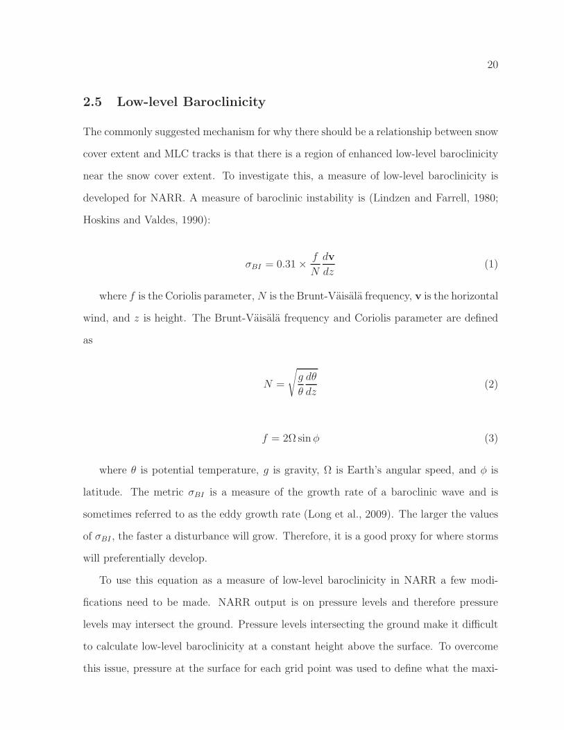
2.5 Low-level Baroclinicity

The commonly suggested mechanism for why there should be a relationship between snow

cover extent and MLC tracks is that there is a region of enhanced low-level baroclinicity

near the snow cover extent. To investigate this, a measure of low-level baroclinicity is

developed for NARR. A measure of baroclinic instability is (Lindzen and Farrell, 1980;

Hoskins and Valdes, 1990):

σBI = 0.31×f

N

dv

dz(1)

where f is the Coriolis parameter, N is the Brunt-Vaisala frequency, v is the horizontal

wind, and z is height. The Brunt-Vaisala frequency and Coriolis parameter are defined

as

N =

√

g

θ

dθ

dz(2)

f = 2Ω sinφ (3)

where θ is potential temperature, g is gravity, Ω is Earth’s angular speed, and φ is

latitude. The metric σBI is a measure of the growth rate of a baroclinic wave and is

sometimes referred to as the eddy growth rate (Long et al., 2009). The larger the values

of σBI , the faster a disturbance will grow. Therefore, it is a good proxy for where storms

will preferentially develop.

To use this equation as a measure of low-level baroclinicity in NARR a few modi-

fications need to be made. NARR output is on pressure levels and therefore pressure

levels may intersect the ground. Pressure levels intersecting the ground make it difficult

to calculate low-level baroclinicity at a constant height above the surface. To overcome

this issue, pressure at the surface for each grid point was used to define what the maxi-

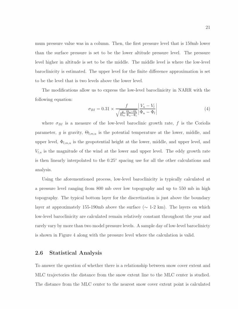
21

mum pressure value was in a column. Then, the first pressure level that is 150mb lower

than the surface pressure is set to be the lower altitude pressure level. The pressure

level higher in altitude is set to be the middle. The middle level is where the low-level

baroclinicity is estimated. The upper level for the finite difference approximation is set

to be the level that is two levels above the lower level.

The modifications allow us to express the low-level baroclinicity in NARR with the

following equation:

σBI = 0.31×f

√

g

Θm

Θu−Θl

Φu−Φl

∣

∣

∣

∣

∣

Vu − Vl

Φu − Φl

∣

∣

∣

∣

∣

(4)

where σBI is a measure of the low-level baroclinic growth rate, f is the Coriolis

parameter, g is gravity, Θl,m,u is the potential temperature at the lower, middle, and

upper level, Φl,m,u is the geopotential height at the lower, middle, and upper level, and

Vl,u is the magnitude of the wind at the lower and upper level. The eddy growth rate

is then linearly interpolated to the 0.25 spacing use for all the other calculations and

analysis.

Using the aforementioned process, low-level baroclinicity is typically calculated at

a pressure level ranging from 800 mb over low topography and up to 550 mb in high

topography. The typical bottom layer for the discretization is just above the boundary

layer at approximately 155-190mb above the surface (∼ 1-2 km). The layers on which

low-level baroclinicity are calculated remain relatively constant throughout the year and

rarely vary by more than two model pressure levels. A sample day of low-level baroclinicty

is shown in Figure 4 along with the pressure level where the calculation is valid.

2.6 Statistical Analysis

To answer the question of whether there is a relationship between snow cover extent and

MLC trajectories the distance from the snow extent line to the MLC center is studied.

The distance from the MLC center to the nearest snow cover extent point is calculated

22

using the snow cover and MLC position on the same day (zero lag). Typically, the

distance calculated is north to south, but in some instances, such as near the Rocky

Mountains, the shortest distance may be east to west oriented. If the MLC center is over

snow, then the distance value is set to be negative. If the MLC is not over snow, then

the distance is set to be positive. This means that negative distances are found north of

the snow extent line, while positive values are found south of the snow extent line.

The distance was calculated for all months, except for June through September, which

were removed. During the summer and early fall, the snow extent approaches the north-

ern edge of our domain. We do not have confidence in the results when the snow extent is

near the edge of our domain due to the inability of our algorithm and model to simulate

snow cover in that region. The results will be discussed with relation to three seasons, the

fall, the winter, and the spring. November is presented as the representative member of

the fall (October and November), January as the winter (December, January, February),

and March as the spring (March, April, May). The fall and spring are sometimes referred

to as the shoulder seasons.

To investigate the significance of the enhanced peaks, distributions of the distances

using shuffled snow cover extent were calculated. The resulting distributions were then

subtracted from the distribution using snow cover and MLC centers in the same year.

Summing the differences between all the distributions shows where the most consistent

change is occurring. It is assumed that shuffling the data will create mostly random noise

that will cancel when summed. Any non-random noise will result in peaks.

23

3 Results

The following section provides general statistics and evaluation of our NARR-derived

snow cover extent and MLC climatology. The relationship between MLC centers and

snow cover extent is investigated and the robustness of the relation is evaluated. Low-

level baroclinicity is studied to determine its role in any coupling between snow cover

and MLCs. Unless otherwise noted, the following analysis was performed for 0000 UTC

01 January 1978 to 2100 UTC 31 December 2010.

3.1 Snow Cover Statistics

Mean latitude of snow cover extent for each day between 125 W and 67 W was cal-

culated. Snow cover extent features a large mean annual cycle ranging from its most

southern extent at 40.2 N in January to its northern most extent in August at 70.1 N.

Mean monthly snow cover extent experiences its largest variability during the spring and

the fall. The most southern monthly mean snow extent occurred in January 1979 at

38.0 N. The single day maximum snow cover extent occurred on February 5th, 1996

when mean longitudinal snow cover extent was 35.4 N.

There is no clear trend in mean monthly latitude of snow cover from 1979-2010 (Fig-

ure 5). Two months (May and December) have a negative slope, which suggests that

mean monthly snow cover extent has shifted farther south. The remaining months all

have positive slopes signaling that snow cover has retreated farther north. The only sta-

tistically significant trends at the 95% confidence level occur in May (p = 0.02), October

(p = 0.0005), and November (p = 0.02). Relaxing confidence to the 90% level does not

add any months.

24

3.2 Snow Cover Extent Evaluation

Our algorithm for snow cover extent was also applied to the SNODAS dataset for 2004

to 2009. The root mean square error (RMSE) between NARR and SNODAS snow cover

extent for each degree longitude from October to May is 4.5. Figure 6 shows frequency

distributions of the difference between NARR and SNODAS. In general, NARR tends to

be farther north than SNODAS. The mean of difference for each longitude (Figure 6a)

is better than the difference in the mean latitudinal extent across all longitude points

(Figure 6b). The winter typically agrees within -0.3 to 1.7 latitude when comparing

each point and the difference of the mean latitude of snow cover extent increases to

0.7 to 2.6. Almost all of the differences greater than 10 occur over mountain ranges.

The largest differences appear in the Rocky Mountains and slightly less frequent large

differences appear in the Sierra Nevada mountain range. Small peaks of large differences

are also seen over the Appalachian Mountains, but not nearly as frequently as other

mountain ranges. Differences greater than 5 exhibit a similar relationship in mountain

ranges. Excluding mountainous areas, the two datasets typically agree within 5 latitude

with NARR tending to have a northern bias as compared to SNODAS.

Summary statistics of our algorithm applied to six years of SNODAS are similar to

32 years of NARR. The maximum monthly mean snow cover extent shifts from January

to February and shifts further south to 39.0 N from the 40.2 N in January in NARR.

The separation between mean monthly snow cover extent between January and February

is smaller for SNODAS (0.1 N) than for NARR (0.5 N). The mean snow extent retreat

from March to May occurs much more slowly in SNODAS (0.9 per month) than NARR

(3.6 per month).

25

3.3 Cyclone Statistics

The following statistics apply to the region between 125 W and 67 W and 20 S to

65 N. It is important to note that storms can both enter and leave our domain because

of the inherent nature of a regional reanalysis product. Therefore, we cannot make any

statements on genesis or the true duration of storms. The statistics provided in this

section are only valid for our region of interest.

The average number of MLCs identified by our algorithm was 1644 per year. The

maximum number of MLCs occurred in 2004 with 1822 identified and the minimum

occurred in 2010 with 1568. The maximum number of storms happened during the sum-

mer and the minimum number of storms occurred during the winter. The reversal from

conventional thinking about the frequency of MLC between the summer and winter is

a result of our limited domain and tracking algorithm. The average duration of identi-

fied MLCs is 23.1 hrs with a maximum average duration of 24.8 hrs in February and a

minimum average duration in July at 20.8 hrs.

Constraining the results by increasing the minimum MLC duration to at least one

day results in an average of 306 per year, a 81.3% reduction. Thus, a majority of our

storms are tracked for a period of nine to twenty-four hours. The maximum number of

storms (333) longer than a day occurred in 1984 and the minimum (277) was observed

in 1980. Requiring longer duration storms shifts the most frequent period of cyclone

activity to the spring (28.2 MLC per month). The summer becomes the month with

the least amount of MLCs at 23.4 per month. The average length of MLCs increases to

50.0 hrs and there is little intermonthly variability (standard deviation of 1.1 hrs).

Increasing the minimum duration to at least 48 hrs (for comparison with other track-

ing methods that relied on 12 hr time steps) results in a 79.7% reduction to an average

of 62.2 storms per year. The average storm duration further increased to 72 hrs and

again there was little variation between months (standard deviation of 1.9 hrs). The

26

longest observed MLC within our domain was in May 1993, lasting for 165hrs (6 days

and 21 hrs).

3.4 Mid-latitude Cyclone Trajectory Evaluation

Our database of MLC trajectories was compared visually to the Atlas of Extratropi-

cal storm tracks. Maps of storm trajectories from NARR were plotted over the storms

from the Atlas of Extratropical Storm Tracks (Chandler and Jonas, 1999) for all months.

Storm trajectories from NARR overlapped a majority of the storm tracks from Chandler

and Jonas (1999). In some cases, the trajectories from Chandler and Jonas (1999) were

represented by two different storms in our NARR database. As expected, due to differ-

ences in selection criteria and resolution, many more storm trajectories were identified

in our NARR database than in the Atlas of Extratropical Storm Tracks. There are some

instances where our algorithm does not identify a trajectory, but the Atlas of Extratrop-

ical Storm Tracks does. Without further investigation, it is unclear if it is missed in our

database or mis-identified by their algorithm.

3.5 Relationship

First, we take a look at storms that last at least 24 hours in order to remove the weakest

MLCs in our database. Analysis of storms shorter than a day will be presented later.

Figure 7a is the histogram of the distance between the snow extent and the MLC centers

for the month of November. The center of the distribution appears to be related to the

snow extent line (zero distance). The maximum frequency occurs just south of the snow

extent line and exhibits a longer tail south of the snow extent than to the north. The

spring has a distribution that is very similar to the fall (Figure 7c). The main difference

in March is a more pronounced peak in frequency just south of the snow extent line.

The enhanced peak in frequency is from about 50-350 km south of the snow extent line.

27

The tail south of the snow extent line is not as large as November, but the frequency

north of the snow extent line retains its shape with only a small increase in magnitude.

The winter displays a similar characteristic to the shoulder seasons with one marked

difference–January (Figure 7b). January has a bimodal distribution with a peak near

the snow extent line and another peak approximately 450-750 km north of the snow

extent line. Possible explanations for the peak north of the snow extent are presented in

the discussion. The common trait among all months is an enhanced frequency of MLCs

in a region 50-350 km south of the snow extent line.

There is approximately a 35% reduction in the number of MLC centers and 25%

reduction in the number of MLCs when requiring storms to last at least 48 hours as

compared to 24 hours. The distance between the MLC center and the snow cover extent

in the fall does not have as pronounced peak as seen in storms lasting longer than a day

(Figure 8a), despite 199 storms that are overlapped between the two time periods. The

same is true for the winter with no enhanced peaks and, in addition, the distributions are

centered around a region approximately 500 km north of the snow extent (Figure 8b).

The spring season still exhibits an enhancement of MLC center frequency in a region of

50-350 km south of the snow extent line (Figure 8c). April and May exhibit stronger

peaks than March.

Taking a broader look, storms lasting longer than nine hours are analyzed. Nine hours

is the theoretical minimum time that produces reliable tracking from our MLC tracking

algorithm. In the fall, there is enhanced frequency of MLC centers near the snow extent

line in a region 0-200 km south of the snow extent (Figure 9a). This region is slightly

farther north than storms lasting longer than one day. The distribution shows a higher

frequency of MLC centers south of the snow extent and the frequency does not decay as

rapidly as compared to storms lasting longer than a day. The winter distributions are

very similar to their 24 hr counterparts. There is a bimodal distribution with one peak

28

in a region 100-300 km south of the snow extent and another peak in a region 600-800

km north of the snow extent (Figure 9b). Spring continues to show an enhanced peak

100-300 km south of the snow extent line (Figure 9c) as it has for all three time criteria.

However, the drop in frequency south of the enhanced region is not as steep as the longer

duration storms.

For an overview of the statistics for all months and subjective analysis of the dis-

tributions please refer to Table 1. Comparing the Atlas of Extratropical Storm Tracks

(Chandler and Jonas, 1999) to snow cover extent instead of using our identified trajecto-

ries from NARR results in similar-looking distributions (not shown). For the remainder

of the analysis, we focus on storms that last longer than a day because they exhibit the

strongest relationship between the snow cover extent and the location of the MLC center.

3.6 Lagged Relationship

It can be argued that one would expect a relationship between mid-latitude cyclone

tracks and snow cover extent because during the cold season it is generally anticipated

that snow would be produced on the northern side of MLCs. Therefore, one may expect

to see MLCs track just south of the snow extent when using no lag time. To investigate

if this is an issue, lagged relationships were looked at with both snow cover extent and

mid-latitude cyclone leading.

The results suggest that it is pre-existing snow cover that is related to the mid-latitude

cyclone tracks and this is shown in Figure 10 , 11, and 12. The middle portion of each

Figure is the distribution for a zero day lag with storms lasting longer than one day. The

top portion is for a two day lag with snow cover leading the MLC and the bottom portion

is for a two day lag with the MLC leading. A two day lag with snow cover leading is

representative of snow cover leading for lags one to five. There is very little difference

between the zero day lag and the other lag times with snow leading. With the snow

29

cover leading the MLCs there is still an enhanced frequency of MLC centers in a region

approximately 50-350 km south of the snow extent line. There is a small shift to left

observed in a few months. A strong leftward shift is seen with MLCs leading the snow

cover extent by two days. The peaks with MLCs leading also tend to be larger, more

pronounced, and nearly centered on zero distance.

3.7 Robustness

Comparing the distribution for the actual year to all other years shows the largest and

most coherent structures in a region just south of the snow extent line (Figure 13). There

are substantial differences in the distributions just south of the snow extent line when

using snow cover extent from all other years. There is increased frequency of mid-latitude

cyclone centers in a region 50-350 km south of the extent line when the snow cover extent

and MLCs are from the same year.

3.8 Low-level Baroclinicity

Normalized mean low-level baroclinicity in 100 km bins surrounding the snow extent are

presented in Figure 14. It is evident that baroclinicity peaks in a region just south of

the snow extent in all months. The structure of baroclinicity is almost identical for all

months with the smallest values in a region south of approximately 1500 km south of

the snow extent and the largest values occurring in a region from the snow extent to

approximately 1000 km south of the snow extent. The fall (Figure 14a) has a stronger

peak than the other months because of much lower baroclinicity values north of the snow

extent as compared to the winter and spring. The results show that the largest values of

low-level baroclinicity occur in a region that roughly coincides with the peaks in MLC

frequency. It is important to note that the enhancement of baroclinicity is much broader

and not as pronounced at the MLC distance distribution peaks.

30

3.9 Variables Relative to Snow Cover Extent

Plots of select variables (albedo, temperature, latent heat flux, and sensible heat flux)

relative to the snow cover extent are shown in Figure 15 for the month of March. The

values represent composite mean daily values for each variable following the snow cover

extent on each day. There is clearly a difference in albedo across the snow extent boundary

(Figure 15a) with values north of the snow extent averaging between 35% to 55% and

values south of the snow extent in the 15% to 25% range. The smaller scale structures

in the albedo are tied to mountains and vegetation. The expected temperature structure

relative to the snow extent is seen and shown in Figure 15b. There is a small enhancement

of temperature gradient near the snow cover extent. Snow cover tends to mute the sensible

(Figure 15c) and latent heat (Figure 15d) fluxes as compared to bare ground and they

exhibit a structure that is related to the snow cover extent edge. The difference in sensible

and latent heat fluxes is setting up a temperature anomaly pattern that is supportive of

baroclinic instability.

31

4 Discussion

The results show that there is an enhanced frequency of MLCs in a region 50-350 km

south of the snow extent. The region of enhanced MLC frequency is also the region

where the largest values of low-level baroclinicity are experienced. In this section we

will first discuss how valid our choice of using NARR is and then explain the features of

the relationship between MLCs and snow cover extent. We will close with a postulation

that snow cover extent may play a role in the northward shift of storm tracks seen under

conditions of ACC.

4.1 NARR Evaluation

NARR snow cover extent and SNODAS snow cover extent compare well when using our

snow cover identification algorithm (RMSE of 4.5). Almost all of the large errors (≥ 5)

occur in mountainous regions and it is likely that those regions dominate the RMSE. For

example, restricting the snow cover extent evaluation to 95 W to 80 W (approximately

the area east of the Rocky Mountains and west of the Appalachian Mountains) reduces

the RMSE to 1.6. The large errors in mountainous regions may be explained by the

grid spacing of the datasets, despite linearly interpolating both datasets to a 0.25 grid.

The quality of the interpolation will depend on the native spatial resolution. SNODAS is

linearly interpolated from 1 km grid spacing to 0.25 (∼ 27 km) and NARR is linearly in-

terpolated from 32 km. Due to a higher spatial resolution, SNODAS is expected to better

represent complex topography and therefore give a better representation of snow cover in

mountainous regions. A better representation of complex topography also explains why

there is a southern bias of SNODAS compared to NARR because our algorithm for the

southern edge of snow cover extent is sensitive to high topography where snow tends to

last longer than surrounding regions.

Trends in 1979-2010 North American snow cover extent are inconclusive because some

32

months (i.e. May and December) show an increase (more southern mean snow extent)

and the other months show a decrease (more northern mean snow extent). A majority of

the trends are not statistically significant. The statistically significant increase in snow

cover extent during May is interesting because it is opposite result of the strong negative

trends seen in Frei et al. (1999) and Brown (2000). The reason for the discrepancy

may be explained by our algorithm because of how it acts in mountainous regions where

snow remains for extended periods of time at high elevations. The algorithm may sense

continuous snow cover in the mountains, but the continental snow cover pattern may

suggest that the snow extent is actually much further north. With ACC in mountainous

regions, SWE is expected to increase due to increased precipitation because they will still

remain below the 0C threshold (Brown and Mote, 2009). Regions with lower elevation

will be more sensitive to AAC because their mean temperatures are closer to the 0C

threshold (Brown and Mote, 2009). Therefore, we expect the continental scale snow

cover to continue to decrease due to rising temperature, but snow at high elevations to

increase. The trend will result in our algorithm increasingly over estimating snow cover

extent. Thus, our algorithm cannot reliably produce trends in snow cover extent due to

inherent biases in mountainous terrain. However, our analysis of snow cover extent to

MLC positions is still valid because the mountainous regions, where the issue is evident,

are a small fraction of our domain. In addition, a similar relationship is seen when

restricting the domain to be east of the Rocky Mountains and west of the Appalachian

Mountains.

Visual comparison shows that our storm database contained most of the storm trajec-

tories identified in the Atalas of Extratropical Storm Tracks (Chandler and Jonas, 1999).

It is difficult to make a direct comparison between our database and other databases

because of (1) differences in temporal and spatial resolutions, (2) different reanalysis

datasets, and (3) lack of absolute “truth” with which to compare. Each method and

33

dataset is tailored to the specific needs of the question being asked. However, we have

confidence that our database is adequate for our needs because the same relationship be-

tween MLC centers and snow cover extent is seen using both our database and the Atlas

of Extratropical Storm Tracks, despite the differences in technique and large differences

in temporal and spatial resolution.

4.2 Relationship Between Snow Cover and MLCs

There is a strong and robust relationship of the distance between MLC centers and the

southern edge of the snow cover extent. The frequency distribution of MLC centers

typically features enhanced peaks in a region south of the snow extent for storms lasting

longer than one day and all the distributions are nearly centered near the snow extent line.

A preferential region for MLC trajectories near the snow extent boundary supports the

ideas postulated in Namias (1962) and Ross and Walsh (1986). From the aforementioned

results, the region can be quantified as being 50-350 km south of the snow extent.

The bimodal distributions seen in a few months (mainly January) can plausibly be

explained by Alberta Clippers. Alberta clippers are fast moving MLCs that are most

commonly found in December and January (Thomas and Martin, 2007). Alberta clippers

are generated in the lee of the Rocky Mountains in Alberta, Canada and generally track

east-southeast toward the north central border of the United States where they then

continue to progress eastward (Thomas and Martin, 2007). The trajectory of an average

Alberta clipper is approximately 600 km to 800 km north of the mean January snow

extent (∼40 N). This region corresponds to the location of the bimodal peak observed

north of the snow over extent in January. The fast-moving nature of these storms is the

reason the bimodal peak becomes less pronounced, as the minimum duration of MLCs

increases.

It can be argued that a close relationship between MLCs and snow cover extent is

34

expected because winter MLCs are likely to deposit snow. Generally, MLCs during the

winter will deposit snow on their north side and produce non-frozen precipitation south

of their center. This precipitation pattern would produce the relationship seen; the MLC

center is just south of the snow cover extent. However, lagged analysis shows that it is

pre-existing snow cover that is related to the MLC trajectories. The differences between

snow cover and MLCs on the same day versus snow cover two days before the MLCs

are small. This is highly suggestive that it is not snow being produced by the MLC

itself. In addition, the relationship with the MLC leading the snow cover is consistent

with the expectation of snow being produced to the north of the center and non-frozen

precipitation to the south. With the MLCs leading the snow cover by two days there is

a shift toward the left in the distributions, indicative of the center moving closer to the

snow edge. This is likely snow deposited by the MLC itself.

It is difficult to determine the significance of the enhanced peaks near the snow extent

because there is no a priori distribution that is expected. To attempt to prove the

enhanced peaks near the snow extent are significant and not a random occurrence, we

computed distributions of the distance between snow cover extent and MLCs using snow

cover from all other years as a way to shuffle the datasets. Summing the distributions

should result in any random noise canceling out. The most coherent structures in the

differences occur in a region 50-350 km south of the snow extent. Outside of the region

south of the boundary, the structures in the differences are not coherent and are of

smaller magnitude. The structures suggest that MLCs in the region just south of the

boundary are closely tied to the snow cover extent for the same year. Therefore, the

relationship between MLC centers and the snow cover extent must have a physical link.

A stronger relationship in the spring is also seen. The peaks observed in the distributions

of distances are largest and the robustness analysis has the largest and most coherent

structures during the spring. This may be attributed to increasing incident solar radiation

35

during the spring. The increase in solar radiation will in turn increase the temperature

contrast between the snow-covered ground and the bare-ground. Segal et al. (1991b)

found that the “snow breeze” was strongest during the spring for this very reason. A

“snow breeze” type circulation and increasing solar radiation resulting in a temperature

contrast are two physical processes that can link the snow cover extent to the MLCs. As

additional evidence toward robustness of the result, the distance relationship is similar

to the distributions seen using the Atlas of Extratopical Storm Tracks (Chandler and

Jonas, 1999) instead of our NARR derived storm positions.

4.3 Physical Mechanism

The commonly postulated (e.g., Namias, 1962; Ross and Walsh, 1986) mechanism for

the relationship between mid-latitude cyclone tracks and snow cover extent is one that is

based on a region of enhanced low-level baroclinicity along the snow cover extent. The

enhanced temperature and moisture gradient setup from the change in surface properties

induces a temperature gradient between the snow covered and the ground without snow

cover. The temperature gradient is a result of a large gradient in surface albedo that

leads to a large difference in absorbed incident solar radiation. The increased tempera-

ture gradient across the snow extent line is then believed to lead to enhanced low-level

baroclinicity. Regions of enhanced baroclinicity are more favorable for MLCs because

the eddy growth rate is enhanced.

The results show that the largest mean baroclinicity values, relative to the snow

extent, are in a region just south of the snow extent. The area of enhanced baroclinicity

is much broader (from approximately the snow extent to 800 km south of the snow

extent) than the peaks observed in MLC cycle frequency relative to the snow extent that

tended to be very pronounced and limited to a few hundred kilometers. The region of

largest baroclinicity just south of the snow extent provides support for the mechanism

36

proposed in Namias (1962) and Ross and Walsh (1986). The region immediately south

of the snow extent will experience maximum eddy growth rates making it a region that

is favorable for MLCs to develop and grow. The region of maximum growth rate is

analogous to the region of maximum baroclinic instability. It is expected that MLCs will

tend to follow regions of maximum baroclinic instability because it is the primary driving

mechanism for them. The region of maximum eddy growth rates coupled with the same

region experiencing maximum cyclone frequency signals that the two are related. It is

not clear from our analysis how this low-level baroclinicity is realized at upper levels. We

speculate that a pre-existing disturbance at upper-levels is need in order to realize the

enhanced baroclinicity at low-levels. The low-level baroclinicity will modify the structure

of the MLC resulting in trajectory changes. More work is needed to understand why the

MLC centers are seen in a region 50-350 km south of the snow extent while the region

of maximum baroclinic instability does not always peak in that region and has a much

broader structure.

With ACC, snow cover extent is expected to decrease (Brown and Mote, 2009) due

to rising global temperatures and there is an observed (IPCC, 2007; Sickmoller et al.,

2000; Wang et al., 2006) and forecast (Bengtsson et al., 2006; Jiang and Perrie, 2007)

northward shift in storm tracks (mainly over the North Atlantic and North Pacific).

If the relationship between MLC centers and snow cover extent remains constant with

ACC, then a northward shift of MLCs over continents would be expected given a shift

northward in snow cover extent. The shift northward of snow cover over continents

may also play a role in the northward shift seen in the ocean basins east of continents.

Hoskins and Valdes (1990) demonstrated that increased baroclinicity generated off the

east coast of continents was important to the start of storm tracks in those regions.

Ross and Walsh (1986) found that enhanced baroclinicity near coastal boundaries due

to increased snow cover is important to MLC trajectories. Therefore, as snow cover

37

extent moves northward over continents we speculate that this will move the region of

enhanced baroclinicity at the coast northward too. With this northward shift and that

the North Atlantic and North Pacific storm tracks are sensitive to the region of enhanced

baroclinicity we postulate that snow cover retreat over continents may play a role in the

northward shift seen in ocean basins.

38

5 Conclusion

AMLC identification and tracking method was developed using high temporal and spatial

resolution NARR output. A simple algorithm for determining the southern extent of

snow cover in North America was created so the MLC centers could be compared to it.

Investigation of the role snow cover extent has on MLC trajectories showed that there is

an enhanced region of MLC frequency 50-350 km south of the snow cover extent. The

relationship appears to be driven by low-level baroclinicity that is at its maximum in

this region. Increased low-level baroclinicity is believed to be driven by the increased

temperature gradient across the boundary due to differences in absorbed solar radiation.

The relationship between MLC centers and snow cover extent is shown to be robust by

shuffling years of snow cover and showing that the largest and most coherent changes

occur in the region of enhanced MLC frequency. In addition, the relationship is insensitive

to the MLC database used. The close relationship between MLC centers and snow cover

extent may play a role in the northward shift of storm tracks seen with ACC. Snow cover

is found to lead the MLC centers, and thus with a northward retreat of snow cover extent

due to ACC we expect a similar northward shift in MLC tracks over the North American

continent.

5.1 Future Work

Now that a statistical relationship has been shown, it will be useful to further investigate

the relationship using a numerical model. A numerical model will reduce a lot of the

uncertainty of the statistical analysis because a better cause and effect relationship can

be established. In addition, it will allow us to explain why the MLC center is where it

is given the location of the enhanced low-level baroclinicity. There are two setups we

feel will be useful in studying the relationship further. The first is to use an idealized

MLC with no topography. This type of experiment will allow varying distances of snow

39

cover extent from the mid-latitude cyclone center. The MLCs can be tracked, using a

similar algorithm presented in this paper or a more sophisticated one because it will be

less computationally intensive, and compared for varying degrees of snow cover extent.

Comparing the snow covered runs to a bare-ground control run will allow one to see how

the trajectory is modified due to the snow cover feedbacks. The second is to do reanalysis

of real MLCs with varying degrees of snow cover. This is very similar to the work of

Elguindi et al. (2005), but with the important difference that it is small variations of

snow cover extent. This type of experiment will allow topography and other feedbacks

not in the idealized case to have an impact. We hypothesize that in the real world case

there will be less of a change in MLC trajectory than in the idealized case because of the

increased complexity of the system. It has also been suggested that some of the analysis

we have performed be segregated beyond just months to see if the relationship is stronger

or weaker in certain situations than others. For example, one can separate the results by

ENSO phases to see if ENSO plays a significant role in the relationship. Also, looking at

the relationship segregated by mean latitude of the snow extent line may provide some

interesting results related to any climatological factors driving the relationship or if our

relationship is only from storms like the ones discussed in Namias (1962) (when the snow

cover extent it near coastal boundaries). A better understanding of the physical processes

involved will allow for a better assessment of what changes to MLC trajectories can be

expected with ACC.

40

References

Alexander, P. and G. Gong, 2011: Modeled surface air temperature response to snowdepth variability. Journal of Geophysical Research, 116 (D14), 1–14, doi:10.1029/2010JD014908.

Allen, R. J. and C. S. Zender, 2011a: Forcing of the Arctic Oscillation by Eurasian SnowCover. Journal of Climate, 24 (24), 6528–6539, doi:10.1175/2011JCLI4157.1.

Allen, R. J. and C. S. Zender, 2011b: The role of eastern Siberian snow and soil moistureanomalies in quasi-biennial persistence of the Arctic and North Atlantic Oscillations.Journal of Geophysical Research, 116 (D16), 1–12, doi:10.1029/2010JD015311.

Alpert, P., B. U. Neeman, and Y. Shay-El, 1990: Climatological analysis of Mediter-ranean cyclones using ECMWF data. Tellus A, 42 (1), 65–77, doi:10.1034/j.1600-0870.1990.00007.x.

Baker, D. G., D. L. Ruschy, R. H. Skaggs, and D. B. Wall, 1992: Air Temperature andRadiation Depressions Associated with a Snow Cover. Journal of Applied Meteorology,31 (3), 247–254, doi:10.1175/1520-0450(1992)031〈0247:ATARDA〉2.0.CO;2.

Barrett, A., 2003: National Operational Hydrologic Remote Sensing Center Snow DataAssimilation System (SNODAS) Products at NSIDC. SIDC Special Report 11. Tech.rep., National Snow and Ice Data Center, 19 pp., Boulder, CO.

Bauer, K. G. and J. a. Dutton, 1962: Albedo Variations Measured from an Airplaneover Several Types of Surface. Journal of Geophysical Research, 67 (6), 2367–2376,doi:10.1029/JZ067i006p02367.

Bauer, M. and A. D. Del Genio, 2006: Composite Analysis of Winter Cyclones in aGCM: Influence on Climatological Humidity. Journal of Climate, 19 (9), 1652–1672,doi:10.1175/JCLI3690.1.

BENESTAD, R. E. and D. CHEN, 2006: The use of a calculus-based cyclone iden-tification method for generating storm statistics. Tellus A, 58 (4), 473–486, doi:10.1111/j.1600-0870.2006.00191.x.

Bengtsson, L., K. I. Hodges, and E. Roeckner, 2006: Storm Tracks and Climate Change.Journal of Climate, 19 (15), 3518–3543, doi:10.1175/JCLI3815.1.

Blackmon, M. L., 1976: A Climatological Spectral Study of the 500 mb GeopotentialHeight of the Northern Hemisphere. Journal of the Atmospheric Sciences, 33 (8),1607–1623, doi:10.1175/1520-0469(1976)033〈1607:ACSSOT〉2.0.CO;2.

Blender, R., K. Fraedrich, and F. Lunkeit, 1997: Identification of cyclone-track regimes inthe North Atlantic. Quarterly Journal of the Royal Meteorological Society, 123 (539),727–741, doi:10.1002/qj.49712353910.

41

Blender, R. and M. Schubert, 2000: Cyclone Tracking in Different Spatial and Tempo-ral Resolutions. Monthly Weather Review, 128 (2), 377, doi:10.1175/1520-0493(2000)128〈0377:CTIDSA〉2.0.CO;2.

Brown, R. D., 2000: Northern Hemisphere Snow Cover Variability and Change, 191597.Journal of Climate, 13 (13), 2339–2355, doi:10.1175/1520-0442(2000)013〈2339:NHSCVA〉2.0.CO;2.

Brown, R. D. and R. L. Armstrong, 2008: Snow-cover data: measurment, products,and sources. Snow and Climate: Physical Processes, Surface Energy Exchange and

Modeling, R. Armstrong and E. Brun, Eds., Cambridge University Press, New York,NY, chap. 5, 181–216.

Brown, R. D. and P. W. Mote, 2009: The Response of Northern Hemisphere SnowCover to a Changing Climate*. Journal of Climate, 22 (8), 2124–2145, doi:10.1175/2008JCLI2665.1.

Cannon, A. J., 2012: Regression-Guided Clustering: A Semisupervised Method forCirculation-to-Environment Synoptic Classification. Journal of Applied Meteorology

and Climatology, 51 (2), 185–190, doi:10.1175/JAMC-D-11-0155.1.

Chandler, M. and J. Jonas, 1999: Atlas of extratropical storm tracks (1961-1998). Tech.rep. URL http://www.giss.nasa.gov/data/stormtracks.

Chang, A. T. C., J. Foster, and D. K. Hall, 1987: Nimbus-7 SMMR derived global snowcover parameters. Annals of Glaciology, 9, 39–44.

Chang, E. K. M., S. Lee, and K. L. Swanson, 2002: Storm Track Dynamics. Journal ofClimate, 15 (16), 2163–2183, doi:10.1175/1520-0442(2002)015〈02163:STD〉2.0.CO;2.

Cohen, J. and D. Entekhabi, 2001: The influence of snow cover on northern hemi-sphere climate variability. Atmosphere-Ocean, 39 (1), 35–53, doi:10.1080/07055900.2001.9649665.

Cohen, J. and D. Rind, 1991: The Effect of Snow Cover on the Climate. Journal ofClimate, 4 (7), 689–706, doi:10.1175/1520-0442(1991)004〈0689:TEOSCO〉2.0.CO;2.

Dery, S. J. and R. D. Brown, 2007: Recent Northern Hemisphere snow cover extenttrends and implications for the snow-albedo feedback. Geophysical Research Letters,34 (22), 2–7, doi:10.1029/2007GL031474.

Dewey, K. F., 1977: Daily Maximum and Minimum Temperature Forecasts and theInfluence of Snow Cover. Monthly Weather Review, 105 (12), 1594–1597, doi:10.1175/1520-0493(1977)105〈1594:DMAMTF〉2.0.CO;2.

Dutra, E., C. Schar, P. Viterbo, and P. M. a. Miranda, 2011: Land-atmosphere couplingassociated with snow cover. Geophysical Research Letters, 38 (15), 1–5, doi:10.1029/2011GL048435.

42

Elguindi, N., B. Hanson, and D. Leathers, 2005: The Effects of Snow Cover on Mid-latitude Cyclones in the Great Plains. Journal of Hydrometeorology, 6 (3), 263–279,doi:10.1175/JHM415.1.

Ellis, A. W. and D. J. Leathers, 1998: The effects of a discontinuous snow cover onlower atmospheric temperature and energy flux patterns. Geophysical Research Letters,25 (12), 2161, doi:10.1029/98GL01582.

Ellis, A. W. and D. J. Leathers, 1999: Analysis of Cold Airmass Temperature Modifica-tion across the U.S. Great Plains as a Consequence of Snow Depth and Albedo. Jour-nal of Applied Meteorology, 38 (6), 696–711, doi:10.1175/1520-0450(1999)038〈0696:AOCATM〉2.0.CO;2.

Finnis, J., M. M. Holland, M. C. Serreze, and J. J. Cassano, 2007: Response of North-ern Hemisphere extratropical cyclone activity and associated precipitation to climatechange, as represented by the Community Climate System Model. Journal of Geophys-

ical Research, 112 (G4), 1–14, doi:10.1029/2006JG000286.

Fletcher, C. G., S. C. Hardiman, P. J. Kushner, and J. Cohen, 2009: The DynamicalResponse to Snow Cover Perturbations in a Large Ensemble of Atmospheric GCMIntegrations. Journal of Climate, 22 (5), 1208–1222, doi:10.1175/2008JCLI2505.1.

Frei, A., D. a. Robinson, and M. G. Hughes, 1999: North American snow extent:19001994. International Journal of Climatology, 19 (14), 1517–1534, doi:10.1002/(SICI)1097-0088(19991130)19:14〈1517::AID-JOC437〉3.3.CO;2-9.

Geng, Q. and M. Sugi, 2001: Variability of the North Atlantic Cyclone Activity in WinterAnalyzed from NCEPNCAR Reanalysis Data. Journal of Climate, 14 (18), 3863–3873,doi:10.1175/1520-0442(2001)014〈3863:VOTNAC〉2.0.CO;2.

Grigoriev, S., S. Gulev, and O. Zolina, 2000: Innovative software facilitates cyclonetracking and analysis. Eos, Transactions American Geophysical Union, 81 (16), 170–170, doi:10.1029/00EO00117.

Grody, N. and A. Basist, 1996: Global identification of snowcover using SSM/I mea-surements. IEEE Transactions on Geoscience and Remote Sensing, 34 (1), 237–249,doi:10.1109/36.481908.

Gulev, S. K., O. Zolina, and S. Grigoriev, 2001: Extratropical cyclone variability in theNorthern Hemisphere winter from the NCEP/NCAR reanalysis data. Climate Dynam-

ics, 17 (10), 795–809, doi:10.1007/s003820000145.

Haak, U. and U. Ulbrich, 1996: Verification of an objective cyclone climatology for theNorth Atlantic. Meteorologische Zeitschrift, 5, 24–30.

Hall, D. K., G. A. Riggs, and V. V. Salomonson, 1995: Development of methods formapping global snow cover using moderate resolution imaging spectroradiometer data.Remote Sensing of Environment, 54 (2), 127–140, doi:10.1016/0034-4257(95)00137-P.

43

Hewson, T. D. and H. a. Titley, 2010: Objective identification, typing and tracking ofthe complete life-cycles of cyclonic features at high spatial resolution. Meteorological

Applications, 17 (3), 355–381, doi:10.1002/met.204.

Hodges, K. I., 1994: A General Method for Tracking Analysis and Its Application toMeteorological Data. Monthly Weather Review, 122 (11), 2573–2586, doi:10.1175/1520-0493(1994)122〈2573:AGMFTA〉2.0.CO;2.

Hodges, K. I., B. J. Hoskins, J. Boyle, and C. Thorncroft, 2003: A Comparisonof Recent Reanalysis Datasets Using Objective Feature Tracking: Storm Tracksand Tropical Easterly Waves. Monthly Weather Review, 131 (9), 2012–2037, doi:10.1175/1520-0493(2003)131〈2012:ACORRD〉2.0.CO;2.

Hoskins, B. J. and K. I. Hodges, 2002: New Perspectives on the Northern HemisphereWinter Storm Tracks. Journal of the Atmospheric Sciences, 59 (6), 1041–1061, doi:10.1175/1520-0469(2002)059〈1041:NPOTNH〉2.0.CO;2.

Hoskins, B. J. and P. J. Valdes, 1990: On the Existence of Storm-Tracks. Journal ofthe Atmospheric Sciences, 47 (15), 1854–1864, doi:10.1175/1520-0469(1990)047〈1854:OTEOST〉2.0.CO;2.

Inatsu, M., 2009: The neighbor enclosed area tracking algorithm for extratropicalwintertime cyclones. Atmospheric Science Letters, 272 (October), n/a–n/a, doi:10.1002/asl.238.

IPCC, 2007: Climate Change 2007: The Physical Science Basis. Contribution of Working

Group I to the Fourth Assessment Report of the Intergovernmental Panel on Cliamte

Change. Cambridge University Press, New York, NY, 996 pp.

Jiang, J. and W. Perrie, 2007: The Impacts of Climate Change on Autumn North AtlanticMidlatitude Cyclones. Journal of Climate, 20 (7), 1174–1187, doi:10.1175/JCLI4058.1.

Johnson, R. H., G. S. Young, J. J. Toth, and R. M. Zehr, 1984: Mesoscale WeatherEffects of Variable Snow Cover over Northeast Colorado. Monthly Weather Review,112 (6), 1141–1152, doi:10.1175/1520-0493(1984)112〈1141:MWEOVS〉2.0.CO;2.

Kaspi, Y. and T. Schneider, 2011: Downstream Self-Destruction of Storm Tracks. Journalof the Atmospheric Sciences, 68 (10), 2459–2464, doi:10.1175/JAS-D-10-05002.1.

Klein, W., 1957: Principal Tracks and Mean Frequencies of Cyclones and Anticyclones in

the Northern Hemisphere, Research Paper No. 40. U.S. Weather Bureau, Washington,DC.

Klingaman, N. P., B. Hanson, and D. J. Leathers, 2008: A Teleconnection between ForcedGreat Plains Snow Cover and European Winter Climate. Journal of Climate, 21 (11),2466–2483, doi:10.1175/2007JCLI1672.1.

44

Konig, W., R. Sausen, and F. Sielmann, 1993: Objective Identification of Cy-clones in GCM Simulations. Journal of Climate, 6 (12), 2217–2231, doi:10.1175/1520-0442(1993)006〈2217:OIOCIG〉2.0.CO;2.

Kopp, T. J. and R. B. Kiess, 1996: The Air Force Global Weather Central Snow analysisModel. 15th Conf. on Weather Analysis and Forecasting, Amer. Meteor. Soc., Norfolk,VA, 220–222.

Kunkel, K. E., M. a. Palecki, K. G. Hubbard, D. a. Robinson, K. T. Redmond, andD. R. Easterling, 2007: Trend Identification in Twentieth-Century U.S. Snowfall: TheChallenges. Journal of Atmospheric and Oceanic Technology, 24 (1), 64–73, doi:10.1175/JTECH2017.1.

Lambert, S. J., 1988: A Cyclone Climatology of the Canadian Climate Centre GeneralCirculation Model. Journal of Climate, 1 (1), 109–115, doi:10.1175/1520-0442(1988)001〈0109:ACCOTC〉2.0.CO;2.

Leathers, D. J., T. L. Mote, A. J. Grundstein, D. a. Robinson, K. Felter, K. Conrad, andL. Sedywitz, 2002: Associations between continental-scale snow cover anomalies and airmass frequencies across eastern North America. International Journal of Climatology,22 (12), 1473–1494, doi:10.1002/joc.807.

Lindzen, R. S. and B. Farrell, 1980: A Simple Approximate Result for the MaximumGrowth Rate of Baroclinic Instabilities. Journal of the Atmospheric Sciences, 37 (7),1648–1654, doi:10.1175/1520-0469(1980)037〈1648:ASARFT〉2.0.CO;2.

Lionello, P., F. Dalan, and E. Elvini, 2002: Cyclones in the Mediterranean region: thepresent and the doubled CO2 climate scenarios. Climate Research, 22, 147–159, doi:10.3354/cr022147.

Long, Z., W. Perrie, J. Gyakum, R. Laprise, and D. Caya, 2009: Scenario changes inthe climatology of winter midlatitude cyclone activity over eastern North Americaand the Northwest Atlantic. Journal of Geophysical Research, 114 (D12), 1–13, doi:10.1029/2008JD010869.

Matson, M. and D. R. Wiesnet, 1981: New data base for climate studies. Nature,289 (5797), 451–456, doi:10.1038/289451a0.

Matsumura, S. and K. Yamazaki, 2012: Eurasian Subarctic Summer Climate in Re-sponse to Anomalous Snow Cover. Journal of Climate, 25 (4), 1305–1317, doi:10.1175/2011JCLI4116.1.

Matsumura, S., K. Yamazaki, and T. Tokioka, 2010: Summertime land-atmosphere inter-actions in response to anomalous springtime snow cover in northern Eurasia. Journalof Geophysical Research, 115 (D20), 1–13, doi:10.1029/2009JD012342.

Mesinger, F., et al., 2006: North American Regional Reanalysis. Bulletin of the American

Meteorological Society, 87 (3), 343–360, doi:10.1175/BAMS-87-3-343.

45

Mote, T. L., 2008: On the Role of Snow Cover in Depressing Air Temperature. Journal ofApplied Meteorology and Climatology, 47 (7), 2008–2022, doi:10.1175/2007JAMC1823.1.

Murray, R. and I. Simmonds, 1991: A numerical scheme for tracking cyclone centres fromdigital data. Part I: Development and operation of the scheme. Australian Meteorolog-

ical Magazine, 39 (3), 155–166.

Namias, J., 1962: Influences of abnormal heat sources and sinks on atmospheric behavior.Int. Symp. on Numerical Weather Prediction, Meteorological Society of Japan, Tokyo,Japan, 615–627.

Namias, J., 1978: Multiple Causes of the North American Abnormal Winter 197677.Monthly Weather Review, 106 (3), 279–295, doi:10.1175/1520-0493(1978)106〈0279:MCOTNA〉2.0.CO;2.

Namias, J., 1985: Some Empirical Evidence for the Influence of Snow Cover onTemperature and Precipitation. Monthly Weather Review, 113 (9), 1542–1553, doi:10.1175/1520-0493(1985)113〈1542:SEEFTI〉2.0.CO;2.

National Centers for Environmental Prediction, 2007: Regional Reanalysis Questions andAnswers. URL http://www.emc.ncep.noaa.gov/mmb/rreanl/faq.html, URL http:

//www.emc.ncep.noaa.gov/mmb/rreanl/faq.html.

Nghiem, S., 2001: Global snow cover monitoring with spaceborne K/sub u/-band scat-terometer. IEEE Transactions on Geoscience and Remote Sensing, 39 (10), 2118–2134, doi:10.1109/36.957275.

Ross, B. and J. E. Walsh, 1986: Synoptic-Scale Influences of Snow Cover and SeaIce. Monthly Weather Review, 114 (10), 1795–1810, doi:10.1175/1520-0493(1986)114〈1795:SSIOSC〉2.0.CO;2.

Segal, M., J. H. Cramer, R. A. Pielke, J. R. Garratt, and P. Hildebrand, 1991a: Obser-vational Evaluation of the Snow Breeze. Monthly Weather Review, 119 (2), 412–424,doi:10.1175/1520-0493(1991)119〈0412:OEOTSB〉2.0.CO;2.

Segal, M., J. R. Garratt, R. A. Pielke, and Z. Ye, 1991b: Scaling and Numerical ModelEvaluation of Snow-Cover Effects on the Generation and Modification of DaytimeMesoscale Circulations. Journal of the Atmospheric Sciences, 48 (8), 1024–1042, doi:10.1175/1520-0469(1991)048〈1024:SANMEO〉2.0.CO;2.

Sickmoller, M., R. Blender, and K. Fraedrich, 2000: Observed winter cyclone tracks inthe northern hemisphere in re-analysed ECMWF data. Quarterly Journal of the Royal

Meteorological Society, 126 (563), 591–620, doi:10.1256/smsqj.56310.

Sinclair, M. R., 1997: Objective Identification of Cyclones and Their Circulation In-tensity, and Climatology. Weather and Forecasting, 12 (3), 595–612, doi:10.1175/1520-0434(1997)012〈0595:OIOCAT〉2.0.CO;2.

46

Sobolowski, S., G. Gong, and M. Ting, 2007: Northern Hemisphere winter climate vari-ability: Response to North American snow cover anomalies and orography. Geophysical

Research Letters, 34 (16), 2–6, doi:10.1029/2007GL030573.

Sobolowski, S., G. Gong, and M. Ting, 2010: Modeled Climate State and DynamicResponses to Anomalous North American Snow Cover. Journal of Climate, 23 (3),785–799, doi:10.1175/2009JCLI3219.1.

Sobolowski, S., G. Gong, and M. Ting, 2011: Investigating the Linear and NonlinearStationary Wave Response to Anomalous North American Snow Cover. Journal of theAtmospheric Sciences, 68 (4), 904–917, doi:10.1175/2010JAS3581.1.

Taylor, C. M., R. J. Harding, R. A. Pielke, P. L. Vidale, R. L. Walko, and J. W. Pomeroy,1998: Snow breezes in the boreal forest. Journal of Geophysical Research, 103 (D18),23 087–23 101, doi:10.1029/98JD02004.

Thomas, B. C. and J. E. Martin, 2007: A Synoptic Climatology and CompositeAnalysis of the Alberta Clipper. Weather and Forecasting, 22 (2), 315–333, doi:10.1175/WAF982.1.

Ulbrich, U., G. C. Leckebusch, and J. G. Pinto, 2009: Extra-tropical cyclones in thepresent and future climate: a review. Theoretical and Applied Climatology, 96 (1-2),117–131, doi:10.1007/s00704-008-0083-8.

Vavrus, S., 2007: The role of terrestrial snow cover in the climate system. Climate Dy-

namics, 29 (1), 73–88, doi:10.1007/s00382-007-0226-0.

Wallace, J. M. and P. V. Hobbs, 2006: Atmospheric science: an introductory survey. 2ded., International Geophysics Series 92, Academic press, 484 pp.

Walland, D. J. and I. Simmonds, 1996: Modelled atmospheric response to changes inNorthern Hemisphere snow cover. Climate Dynamics, 13 (1), 25–34, doi:10.1007/s003820050150.

Walland, D. J. and I. Simmonds, 1997: North American and Eurasian snow cover co-variability. Tellus A, 49 (4), 503–512, doi:10.1034/j.1600-0870.1997.t01-3-00007.x.

Walsh, J. E., 1984: Snow Cover and Atmospheric Variability: Changes in the snowcovering the earth’s surface affect both daily weather and long-term climate. American

Scientist, 72 (1), 50–57.

Walsh, J. E., D. R. Tucek, and M. R. Peterson, 1982: Seasonal Snow Cover andShort-Term Climatic Fluctuations over the United States. Monthly Weather Review,110 (10), 1474–1486, doi:10.1175/1520-0493(1982)110〈1474:SSCAST〉2.0.CO;2.

Wang, X. L., V. R. Swail, and F. W. Zwiers, 2006: Climatology and Changes of Extra-tropical Cyclone Activity: Comparison of ERA-40 with NCEPNCAR Reanalysis for19582001. Journal of Climate, 19 (13), 3145–3166, doi:10.1175/JCLI3781.1.

47

Wojcik, G. S. and D. S. Wilks, 1992: Temperature Forecast Biases Associated withSnow Cover in the Northeast. Weather and Forecasting, 7 (3), 501–506, doi:10.1175/1520-0434(1992)007〈0501:TFBAWS〉2.0.CO;2.

Zhang, Y., T. Li, and B. Wang, 2004: Decadal Change of the Spring Snow Depth over theTibetan Plateau: The Associated Circulation and Influence on the East Asian Sum-mer Monsoon*. Journal of Climate, 17 (14), 2780–2793, doi:10.1175/1520-0442(2004)017〈2780:DCOTSS〉2.0.CO;2.

48

Figure 1: A simple schematic showing the properties induced by snow-covered groundand ground without snow-cover. The gray line is the estimated boundary layer heightand the vertical dotted blue line is the snow cover extent boundary. The letter “L”is positioned in the region hypothesized for MLC centers to track based on enhancedbaroclinicity near the snow extent.

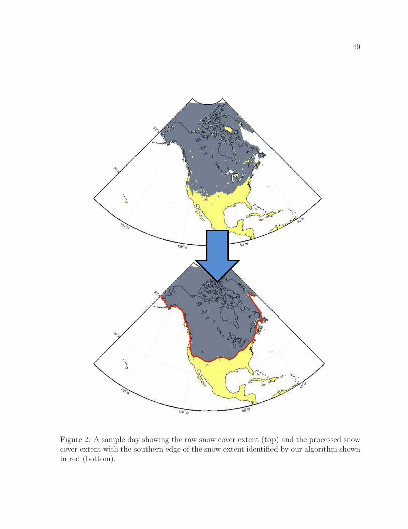
49

Figure 2: A sample day showing the raw snow cover extent (top) and the processed snowcover extent with the southern edge of the snow extent identified by our algorithm shownin red (bottom).

50

Figure 3: A sample identification of MLCs for a single day. The blue dots are pressureminima identified at a fine spatial resolution and the red dots are pressure minima iden-tified at the coarse spatial resolution. The red dots are moved to the closest blue dot todetermine the best estimate of the MLC center.

51

Figure 4: A sample low-level baroclinicity map for a single day. The top panel is thecalculated low-level baroclinicity and the snow cover extent line is shown in white. Thebottom panel is the pressure level at which the low-level baroclinicity was calculated at.

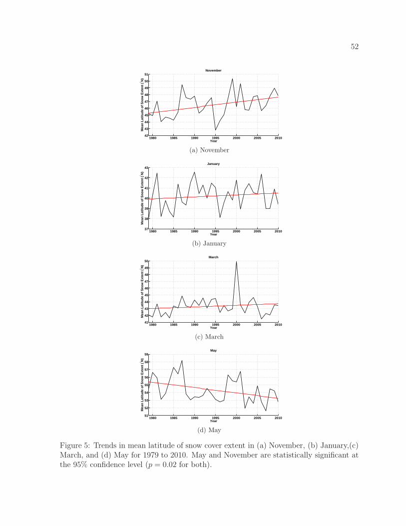
52

1980 1985 1990 1995 2000 2005 201042

43

44

45

46

47

48

49

50

51November

YearM

ean

Latit

ude

of S

now

Ext

ent (

° N)

(a) November

1980 1985 1990 1995 2000 2005 201037

38

39

40

41

42

43January

Year

Mea

n La

titud

e of

Sno

w E

xten

t (° N

)

(b) January

1980 1985 1990 1995 2000 2005 201041

42

43

44

45

46

47

48

49

50March

Year

Mea

n La

titud

e of

Sno

w E

xten

t (° N

)

(c) March

1980 1985 1990 1995 2000 2005 201051

52

53

54

55

56

57

58

59May

Year

Mea

n La

titud

e of

Sno

w E

xten

t (° N

)

(d) May

Figure 5: Trends in mean latitude of snow cover extent in (a) November, (b) January,(c)March, and (d) May for 1979 to 2010. May and November are statistically significant atthe 95% confidence level (p = 0.02 for both).

53

−10 −5 0 5 10 15 20 25 300

50

100

150

200

250

300Winter mean of difference for each longitude

Distance ( ° Latitude)

Fre

quen

cy

(a) October to May Mean of Difference

−10 −5 0 5 10 15 20 25 300

50

100

150

200

250

300Winter difference of mean snow extent

Distance ( ° Latitude)

Fre

quen

cy

(b) October to May Difference of Mean

Figure 6: Comparison of our snow extent algorithm applied to NARR and SNODAS for2004 to 2009. All differences are NARR snow extent minus SNODAS snow extent. (a) isthe mean of the difference for each degree longitude and (b) is the difference of the meanlatitudinal extent across all longitudes for October to May.

54

−3000 −2000 −1000 0 1000 2000 3000 40000

100

200

300

400

500

600November 1979−2010

Distance (km)

Fre

quen

cy

(a) November

−3000 −2000 −1000 0 1000 2000 3000 40000

100

200

300

400

500

600January 1979−2010

Distance (km)

Fre

quen

cy

(b) January

−3000 −2000 −1000 0 1000 2000 3000 40000

100

200

300

400

500

600March 1979−2010

Distance (km)

Fre

quen

cy

(c) March

Figure 7: MLC center distances from snow extent for storms lasting longer than 24 hrs in(a) November, (b) March, and (c) March for 1979 to 2010. Negative distances are MLCcenters that are over snow and positive distances are MLC centers that are over groundwithout snow.

55

−3000 −2000 −1000 0 1000 2000 3000 40000

50

100

150

200

November 1979−2010

Distance (km)

Fre

quen

cy

(a) November

−3000 −2000 −1000 0 1000 2000 3000 40000

50

100

150

200

January 1979−2010

Distance (km)

Fre

quen

cy

(b) January

−3000 −2000 −1000 0 1000 2000 3000 40000

50

100

150

200

March 1979−2010

Distance (km)

Fre

quen

cy

(c) March

Figure 8: MLC center distance from snow extent for storms lasting longer than 48 hrs in(a) November, (b) March, and (c) March for 1979 to 2010. Negative distances are MLCcenters that are over snow and positive distances are MLC centers that are over groundwithout snow.

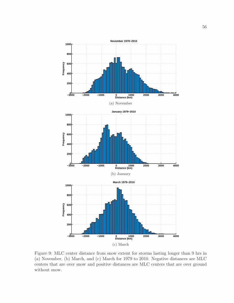
56

−3000 −2000 −1000 0 1000 2000 3000 40000

200

400

600

800

1000November 1979−2010

Distance (km)

Fre

quen

cy

(a) November

−3000 −2000 −1000 0 1000 2000 3000 40000

200

400

600

800

1000January 1979−2010

Distance (km)

Fre

quen

cy

(b) January

−3000 −2000 −1000 0 1000 2000 3000 40000

200

400

600

800

1000March 1979−2010

Distance (km)

Fre

quen

cy

(c) March

Figure 9: MLC center distance from snow extent for storms lasting longer than 9 hrs in(a) November, (b) March, and (c) March for 1979 to 2010. Negative distances are MLCcenters that are over snow and positive distances are MLC centers that are over groundwithout snow.

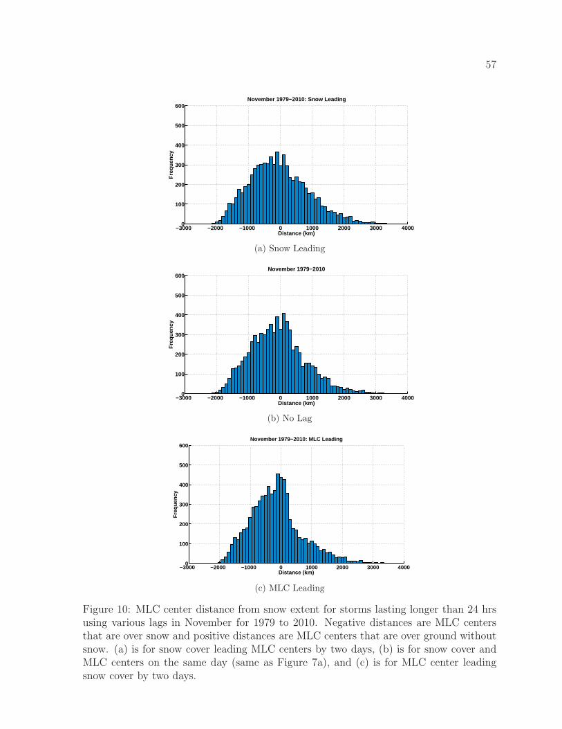
57

−3000 −2000 −1000 0 1000 2000 3000 40000

100

200

300

400

500

600November 1979−2010: Snow Leading

Distance (km)

Fre

quen

cy

(a) Snow Leading

−3000 −2000 −1000 0 1000 2000 3000 40000

100

200

300

400

500

600November 1979−2010

Distance (km)

Fre

quen

cy

(b) No Lag

−3000 −2000 −1000 0 1000 2000 3000 40000

100

200

300

400

500

600November 1979−2010: MLC Leading

Distance (km)

Fre

quen

cy

(c) MLC Leading

Figure 10: MLC center distance from snow extent for storms lasting longer than 24 hrsusing various lags in November for 1979 to 2010. Negative distances are MLC centersthat are over snow and positive distances are MLC centers that are over ground withoutsnow. (a) is for snow cover leading MLC centers by two days, (b) is for snow cover andMLC centers on the same day (same as Figure 7a), and (c) is for MLC center leadingsnow cover by two days.

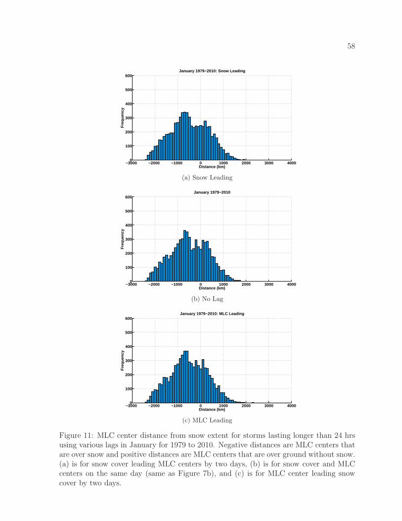
58

−3000 −2000 −1000 0 1000 2000 3000 40000

100

200

300

400

500

600January 1979−2010: Snow Leading

Distance (km)

Fre

quen

cy

(a) Snow Leading

−3000 −2000 −1000 0 1000 2000 3000 40000

100

200

300

400

500

600January 1979−2010

Distance (km)

Fre

quen

cy

(b) No Lag

−3000 −2000 −1000 0 1000 2000 3000 40000

100

200

300

400

500

600January 1979−2010: MLC Leading

Distance (km)

Fre

quen

cy

(c) MLC Leading

Figure 11: MLC center distance from snow extent for storms lasting longer than 24 hrsusing various lags in January for 1979 to 2010. Negative distances are MLC centers thatare over snow and positive distances are MLC centers that are over ground without snow.(a) is for snow cover leading MLC centers by two days, (b) is for snow cover and MLCcenters on the same day (same as Figure 7b), and (c) is for MLC center leading snowcover by two days.

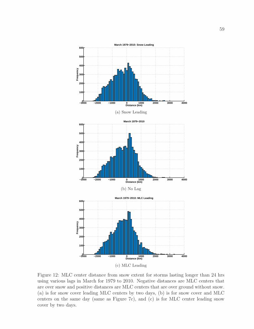
59

−3000 −2000 −1000 0 1000 2000 3000 40000

100

200

300

400

500

600March 1979−2010: Snow Leading

Distance (km)

Fre

quen

cy

(a) Snow Leading

−3000 −2000 −1000 0 1000 2000 3000 40000

100

200

300

400

500

600March 1979−2010

Distance (km)

Fre

quen

cy

(b) No Lag

−3000 −2000 −1000 0 1000 2000 3000 40000

100

200

300

400

500

600March 1979−2010: MLC Leading

Distance (km)

Fre

quen

cy

(c) MLC Leading

Figure 12: MLC center distance from snow extent for storms lasting longer than 24 hrsusing various lags in March for 1979 to 2010. Negative distances are MLC centers thatare over snow and positive distances are MLC centers that are over ground without snow.(a) is for snow cover leading MLC centers by two days, (b) is for snow cover and MLCcenters on the same day (same as Figure 7c), and (c) is for MLC center leading snowcover by two days.

60

−3000 −2000 −1000 0 1000 2000 3000 4000−3000

−2000

−1000

0

1000

2000

3000

4000November 1979−2010

Distance (km)

Fre

quen

cy D

iffer

ence

(a) November

−3000 −2000 −1000 0 1000 2000 3000 4000−3000

−2000

−1000

0

1000

2000

3000

4000January 1979−2010

Distance (km)

Fre

quen

cy D

iffer

ence

(b) January

−3000 −2000 −1000 0 1000 2000 3000 4000−3000

−2000

−1000

0

1000

2000

3000

4000March 1979−2010

Distance (km)

Fre

quen

cy D

iffer

ence

(c) March

Figure 13: The sum of the differences between the distribution for the distance betweenthe MLC using snow for the same year and all other years. Large peaks show systematicbias caused by varying snow cover extent year.

61

−3000 −2000 −1000 0 1000 2000 3000 4000−2

−1.5

−1

−0.5

0

0.5

1

1.5

2November 1979−2010

Distance (km)

Nor

mal

ized

Bar

oclin

icity

(a) November

−3000 −2000 −1000 0 1000 2000 3000 4000−2

−1.5

−1

−0.5

0

0.5

1

1.5

2January 1979−2010

Distance (km)

Nor

mal

ized

Bar

oclin

icity

(b) January

−3000 −2000 −1000 0 1000 2000 3000 4000−2

−1.5

−1

−0.5

0

0.5

1

1.5

2March 1979−2010

Distance (km)

Nor

mal

ized

Bar

oclin

icity

(c) March

Figure 14: Normalized low-level baroclinicity relative to the snow cover extent for (a)November, (b) January, and (c) March.

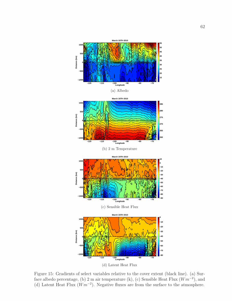
62

−120 −110 −100 −90 −80 −70

−1000

−500

0

500

1000

March 1979−2010

Longitude

Dis

tanc

e (k

m)

15

20

25

30

35

40

45

50

55

(a) Albedo

−120 −110 −100 −90 −80 −70

−1000

−500

0

500

1000

March 1979−2010

Longitude

Dis

tanc

e (k

m)

260

265

270

275

280

285

(b) 2 m Temperature

−120 −110 −100 −90 −80 −70

−1000

−500

0

500

1000

March 1979−2010

Longitude

Dis

tanc

e (k

m)

−90

−80

−70

−60

−50

−40

−30

−20

−10

0

10

(c) Sensible Heat Flux

−120 −110 −100 −90 −80 −70

−1000

−500

0

500

1000

March 1979−2010

Longitude

Dis

tanc

e (k

m)

−80

−70

−60

−50

−40

−30

−20

−10

0

(d) Latent Heat Flux

Figure 15: Gradients of select variables relative to the cover extent (black line). (a) Sur-face albedo percentage, (b) 2 m air temperature (k), (c) Sensible Heat Flux (Wm−2), and(d) Latent Heat Flux (Wm−2). Negative fluxes are from the surface to the atmosphere.

63

Storms Longer than 9 hrsMonth Storms Centers Pk BiM M Pk (km) ER (km)October 4217 7489 Strong No 100 50-250November 3441 7417 Moderate No 200 -150-250December 3318 6599 Moderate Yes 100 50-250January 3270 6916 Weak Yes -600 50-350February 3144 6602 Strong Yes 200 50-250March 3668 8257 Strong No 100 50-350April 4157 8916 Strong No 100 50-350May 5400 8542 Moderate No 100 50-350

Storms Longer than 24 hrsMonth Storms Centers Pk BiM M Pk (km) ER (km)October 802 7489 Strong No 100 50-150November 827 7417 Moderate No 100 -150-250December 802 6599 Weak No 100 noneJanuary 798 6916 Weak Yes -700 50-350February 767 6602 Moderate No 100 50-250March 868 8257 Strong No 200 50-350April 918 8916 Strong No 100 50-350May 920 8542 Strong No 100 -50-250

Storms Longer than 48 hrsMonth Storms Centers Pk BiM M Pk (km) ER (km)October 199 2962 Moderate No 100 -150-350November 199 2813 Weak No -100 noneDecember 147 1948 Weak No -800 noneJanuary 166 2335 Weak No -600 noneFebruary 174 2512 Weak No 100 noneMarch 218 3180 Moderate Yes 100 50-350April 227 3573 Moderate No 200 50-350May 161 2480 Moderate No 100 50-250

Table 1: Summary statistics for MLC lasting longer than 9 hrs, 24 hrs, and 48 hrs.Peakedness (Pk) is a subjective rating of the enhancement of MLC frequency near thesnow cover extent. Bimodal (BiM) distribution is a subjective determination of twodistinct peaks in the distance distributions. The max peak (M Pk) is the center of themost frequent distance bin. The enhanced region (ER) is a subjective determinationof where the distance distributions appear to be more pronounced as compared to asmoothly varying distribution.