Relationship between Rheology and Molecular Structure of ... PhD Thesis .pdf · Relationship between Rheology and Molecular Structure of Innovative Crystalline Elastomers Naveed Ahmad

Thesis for the Degree of Doctor of Philosophy

Relationship between Rheology and Molecular Structure of Innovative Crystalline

Elastomers

Naveed Ahmad

Department of Chemical Engineering

University of Naples

“Federico II”

Italy

March, 2013

Relationship between Rheology and Molecular Structure of Innovative Crystalline

Elastomers

by

Naveed Ahmad

Supervised by

Prof. Nino Grizzuti, Ph.D

Submitted to the Department of Chemical Engineering University of Naples, “Federico II” in partial fulfillment

of the requirements for the degree of Doctor of Philosophy

Prof. Nino Grizzuti (Ph.D. Advisor) …………………………………

Prof. Andrea D'Anna (Ph.D. Co-ordinator) ………………………….

i

Abstract

The study of the rheology of polyolefins based on homogenous metallocenic

catalyst has been mainly devoted to the understanding of material process

ability. When used at a more advanced and sophisticated level, however,

rheology is a useful tool to highlight the details of the polymer

microstructure, such as the chemical stereo-regularity or the degree of chain

branching. Rheology is also used to study the crystallization kinetics of the

polymers and it gives more precise analysis than the conventional techniques

like differential scanning calorimetry (DSC) when the crystallization

kinetics are slow. When cooled below thermodynamic melting temperature,

crystalline polymers undergo crystallization. The early stages of this process

are characterized by the gradual change in the mechanical response of the

material from the liquid to the solid, which is due to the microstructure

evolution of the system. This is one of the great features of the rheological

technique, which distinguishes it from the traditional DSC technique.

In the present research work relationships between rheological parameters

and molecular structure of syndiotactic polypropylenes (sPP) and poly-

1butenes of different stereoregularity are explored by performing oscillatory

shear experiments using ARES rheometer. The rheological response is found

very sensitive to the degree of syndiotacticity of syndiotactic polypropylene,

while in the case of poly-1butenes, it is also found dependent on the

stereoregularity.

Crystallization behavior of a series of syndiotactic polypropylenes of

different degrees of syndiotacticity is investigated by performing both

ii

isothermal and non-isothermal crystallization tests using rheological and

differential scanning calorimetric techniques. The aim is to investigate the

effect of degree of syndiotacticity on the crystallization behavior of the

syndiotactic polypropylene and to couple the rheological methods to more

conventional techniques (such as Differential Scanning Calorimetry).

Crystallization behavior is found strongly dependent on the degree of

syndiotacticity of syndiotactic polypropylene. Good agreement is found

between the results obtained by both the rheological and differential

scanning calorimetric (DSC) methods.

The effect of extensional flow on the crystallization kinetics of sPB is

examined both in the melt and crystal phase by applying different

extensional rates using sentmanat extensional rheometer (SER). Extensional

flow is found to enhance the rate of crystallization in the crystal phase, which

is further proved by the small angle X-Ray scattering experiment (SAX).

iii

Dedicated To

my respected parents, especially to my beloved Father for their

never ending support and for their open-mindedness and endless

support.

iv

Acknowledgement

First and foremost, I would like to give my sincere thanks to ALLAH

SWT, the Almighty, the source of my life and hope for giving me the

strength and wisdom to complete the research.

I am most grateful to my supervisor Prof. Nino Grizzuti for giving me an

opportunity to pursue a PhD degree. Many times, his patience and constant

encouragement has steered me to the right direction. Again, I am most

grateful to Prof. Nino Grizzuti for his support and help in my Research work.

I would also like to thank my Co-supervisors Prof. Giovanni Iannribuerto,

Rossana pasquino and Prof. Giovanni Talarico for his suggestions and help.

I would like to also express my gratitude to all other faculty members of

the Departments of Chemical Engineering and Chemistry for their effort in

helping and providing me with the all chemicals and other experimental tools

that I needed for this research.

Naveed Ahmad

Naples, Italy

March, 2013

v

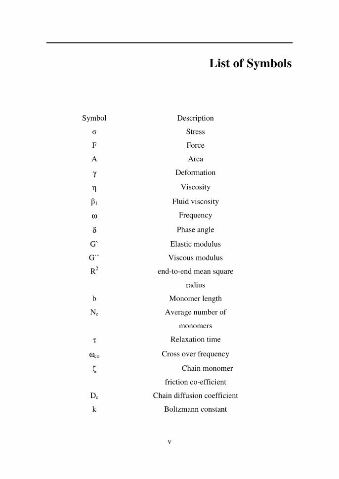
List of Symbols

Symbol Description

σ Stress

F Force

A Area

γ Deformation

η Viscosity

β1 Fluid viscosity

ω Frequency

δ Phase angle

G` Elastic modulus

G`` Viscous modulus

R2 end-to-end mean square

radius

b Monomer length

Ne Average number of

monomers

τ Relaxation time

ωco Cross over frequency

ζ Chain monomer

friction co-efficient

Dc Chain diffusion coefficient

k Boltzmann constant

vi

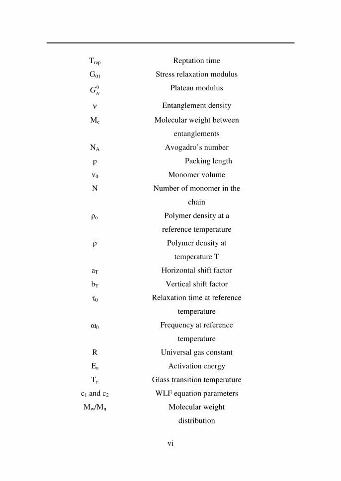
Trep Reptation time

G(t) Stress relaxation modulus

GN

0 Plateau modulus

ν Entanglement density

Me Molecular weight between

entanglements

NA Avogadro’s number

p Packing length

v0 Monomer volume

N Number of monomer in the

chain

ρo Polymer density at a

reference temperature

ρ Polymer density at

temperature T

aT Horizontal shift factor

bT Vertical shift factor

τ0 Relaxation time at reference

temperature

ω0 Frequency at reference

temperature

R Universal gas constant

Ea Activation energy

Tg Glass transition temperature

c1 and c2 WLF equation parameters

Mw/Mn Molecular weight

distribution

vii

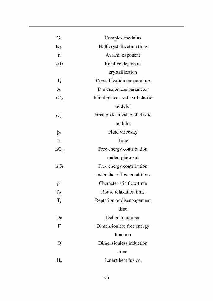
G* Complex modulus

t0.5 Half crystallization time

n Avrami exponent

x(t) Relative degree of

crystallization

Tc Crystallization temperature

A Dimensionless parameter

G`0 Initial plateau value of elastic

modulus

'G ∞ Final plateau value of elastic

modulus

β1 Fluid viscosity

t Time

∆Gq Free energy contribution

under quiescent

∆Gf Free energy contribution

under shear flow conditions

γ-1 Characteristic flow time

TR Rouse relaxation time

Td Reptation or disengagement

time

De Deborah number

Γ Dimensionless free energy

function

Θ Dimensionless induction

time

Ho Latent heat fusion

viii

Tm Melting temperature

*η Complex Viscosity

ῼ Motor rotation rate

( )tFE Tensile force

Sρ Solid state density

( )tA Instantaneous cross sectional

area of the stretched

specimen

D Diameter

H Plate gap

( )tE

+η Tensile stress growth

function

ρL Melt state density

Rg Radius of Gyration

C∞ Characteristic ratio

Vsp Pervaded volume

θ(t) Relative degree of

crystallization

t* Maximum crystallization

time

t1/2 Half crystallization time

k0 Pre-exponential factor

K Rate constant of

crystallization

ix

Table of Contents

ABSTRACT .................................................................................................... I

ACKNOWLEDGEMENT .......................................................................... IV

LIST OF SYMBOLS ................................................................................... V

FIGURE 1.3LIST OF FIGURES............................................................... XI

LIST OF TABLES ................................................................................... XIV

CHAPTER 1: INTRODUCTION ................................................................ 1

1.1. GENERAL INTRODUCTION ................................................................ 1 1.2. RESEARCH OBJECTIVES ................................................................... 5 1.3. LITERATURE REVIEW ....................................................................... 7

1.3.1. Synthesis ..................................................................................... 8 1.3.2. Mechanical Properties ............................................................... 16 1.3.3. Rheology ................................................................................... 22 1.3.4. Crystallization ........................................................................... 49 1.3.5. Flow induced crystallization ..................................................... 54

CHAPTER 2: EXPERIMENTAL METHODS........................................ 63

2.1. LINEAR VISCOELASTICITY ............................................................. 63 2.1.1. Dynamic time sweep test .......................................................... 68 2.1.2. Dynamic strain sweep test ........................................................ 68 2.1.3. Dynamic Frequency Sweep Test .............................................. 69 2.1.4. Dynamic Temperature ramp test ............................................... 69

2.2. EXTENSIONAL FLOW MEASUREMENTS ........................................... 70 2.2.1. Test Setup.................................................................................. 72 2.2.2. Data analysis ............................................................................. 72

2.3. DIFFERENTIAL SCANNING CALORIMETRY ...................................... 74 2.3.1. Working Principle ..................................................................... 74

CHAPTER 3: LINEAR VISCOELASTICITY OF SYNDIOTACTIC

POLYPROPYLENES................................................................................. 76

3.1. INTRODUCTION .............................................................................. 76 3.2. EXPERIMENTAL SECTION ............................................................... 80

3.2.1. Materials ................................................................................... 80

Table of Contents

x

3.2.2. Methodology ............................................................................. 81 3.3. RESULTS AND DISCUSSION ............................................................. 83

3.3.1. Discussion ................................................................................. 94 3.4. CONCLUDING REMARKS ................................................................ 99

CHAPTER 4:QUISCENT CRYSTALLIZATION OF SYNDIOTACTIC

POLYPROPYLENES............................................................................... 100

4.1. INTRODUCTION ............................................................................ 100 4.2. EXPERIMENTAL SECTION ............................................................. 102

4.2.1. Material ................................................................................... 102 4.2.2. Methodology ........................................................................... 103

4.3. RESULTS AND DISCUSSION ........................................................... 106 4.3.1. NON-ISOTHERMAL CRYSTALLIZATION ......................................... 106 4.3.2. ISOTHERMAL CRYSTALLIZATION .................................................. 111 4.3.2.1. RESULTS .................................................................................. 111 4.3.2.2. DISCUSSION ............................................................................. 113 4.4. CONCLUDING REMARKS ............................................................... 124

CHAPTER 5: LINEAR VISCOELASTICITY OF ISOTACTIC,

ATACTIC AND SYNDIOTACTIC POLY-1BUTENES ...................... 126


5.2.1. Material ................................................................................... 127 5.2.2. Methodology ........................................................................... 128 5.2.2.1. Dynamic strain sweep test .................................................. 128 5.2.2.2. Dynamic time sweep test .................................................... 129 5.2.2.3. Dynamic Frequency Sweep Test ........................................ 130

5.3. RESULTS AND DISCUSSION ........................................................... 132 5.4. CONCLUDING REMARKS .............................................................. 136

CHAPTER 6: INFLUENCE OF EXTENSIONAL FLOWS ON THE

CRYSTALLIZATION OF SYNDIOTACTIC POLY-1BUTENE ....... 138


6.2.1. Material ................................................................................... 138 6.2.2. Methodology ........................................................................... 139

6.3. RESULTS AND DISCUSSIONS ......................................................... 140 6.4. CONCLUSION ................................................................................ 150

CHAPTER 7: CONCLUSION................................................................. 152

REFERENCES .......................................................................................... 155

xi

List of Figures

Figure 1.1 Chain structure of syndiotactic (above) and atactic

Polystyrene…………………………………………….

3

Figure 1.2 Chain Initiation step of Ionic polymerization………… 8

Chain Propagation step of Ionic polymerization……… 9

Figure1.3: Chain Propagation step of Ionic polymerization………

9

Figure 1.4 Reaction mechanism of Cationic polymerization

process…………………………………………………

9

Figure 1.5 Chain initiation step during the Co-ordination

polymerization process………………………………..

10

Figure 1.6 Transition state during the Co-ordination

polymerization process………………………………..

10

Figure 1.7 Final step of alkene monomer insertion during the Co-

ordination polymerization process…………………….

11

Figure 1.8 Ziegler Natta catalyst of Cs-symmetry………………... 11

Figure 1.9 Ziegler Natta catalyst of C2-symmetry……………….. 12

Figure 1.10 Mechanism of Chain shuttling polymerization process. 16

Figure 1.11 Engineering data from stress-strain tests……………... 19

Figure 1.12 The Maxwell spring-and-dashpot mechanical analog… 25

Figure 1.13 Frequency response of a poly-butadiene at 27°C.

Dashed lines represent the predictions of the Maxwell

model…………………………………………………..

29

Figure 1.14 Snapshot of the conformations assumed by a single

List of Figures

xii

polymer chain due to Brownian motion………………. 31

Figure 1.15 A schematic view of the entangled melt……………… 33

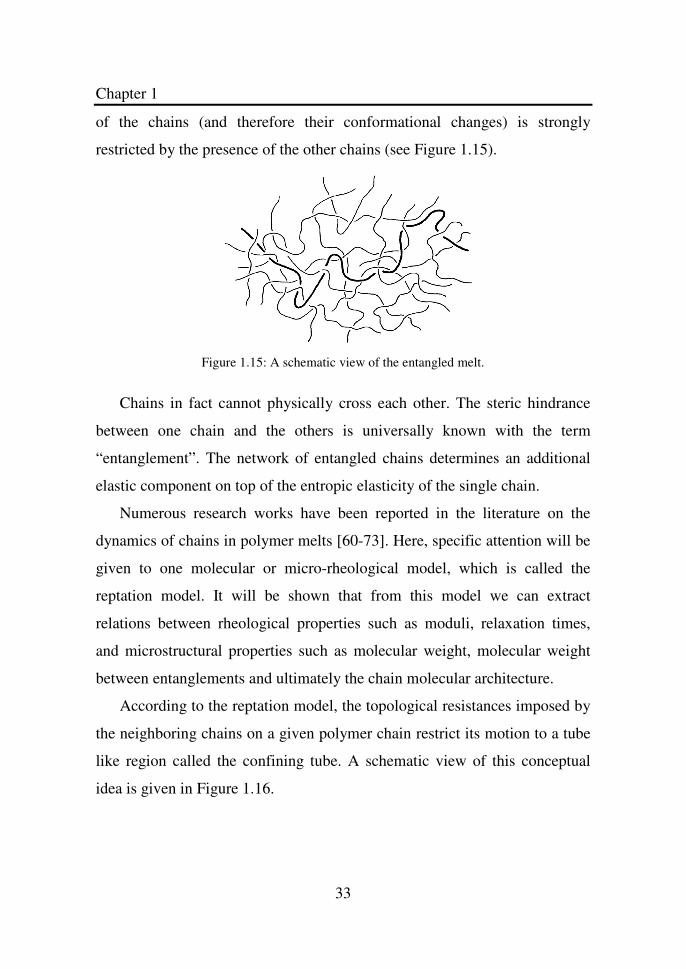
Figure 1.16 A schematic picture of the tube of entanglements. In

(A) the test chain is surrounded by other chains. Only

entanglements are highlighted; in (B) entanglements

are substituted by the tube; in (C) the polymer chain

inside the tube is reduced to its primitive path of N/Ne

segments each of length a……………………………..

34

Figure 1.17 Picture of the chain in the melt. Black dots represent

entanglements due to the presence of other chains. The

red line is the real chain. The broken line is the

primitive path, i.e., the shortest line connecting the

chain ends without violating the topological

constraints……………………………………………..

35

Figure 1.18 Determination of the plateau modulus by the minimum

tan δ method…………………………………………...

47

Figure 1.19 Determination of the plateau modulus by the Van

Gurp-Palmen analysis…………………………………

48

Figure 1.20 DSC curve of Polyethylene…………………………… 50

Figure 1.21 Schematic representation of the flow induced

crystallization………………………………………….

55

Figure 2.1 Rotational rheometer ARES…………………………... 66

Figure 2.2 Parallel plates of 8 mm diameter……………………... 67

Figure 2.3 Dynamic time sweep test set-up screen………………. 68

Figure 2.4 Dynamic strain sweep test set-up screen……………… 68

Figure 2.5 Dynamic frequency sweep test set-up screen…………. 69

Figure 2.6 Dynamic temperature ramp test set-up screen………... 70

List of Figures

xiii

Figure 2.7 Schematic diagram of Sentmanat Extensional

Rheometer……………………………………………..

71

Figure 2.8 Diagram of operation DSC cell……………………….. 75

Figure 3.1 Plot between changes in length of plates vs

Temperature…………………………………………...

82

Figure 3.2 Dynamic time sweep for sPP-9 at 200°C and 10 rad/s.. 84

Figure 3.3 Dynamic time sweep for sPP-9 at 200°C and 10 rad/s.

The thick line is the best fit of Eq. (3.13)……………..

84

Figure 3.4 Dynamic strain sweep test of sPP-9 at 150°C………… 85

Figure 3.5 Dynamic frequency sweep test of sPP-3 at 200°C……. 86

Figure 3.6 Isothermal time sweep for sPP-5 at different

temperatures…………………………………………...

87

Figure 3.7 Spread sheet before shifting……………..…….……… 89

Figure 3.8 Spread sheet after shifting. The vertical shift factor

calculated by the software after density correction is

shown in colum F……………………………………...

89

Figure 3.9 Master curve for sPP-3 at reference temperature of

200oC…………………………………………………..

90

Figure 3.10 Master curve of the loss modulus for sPP-3 on a

linear-log scale………………………………………...

90

Figure 3.11 Master curve for sPP-5………………………………... 92

Figure 3.12 Master curve of the loss modulus for sPP-5 on a

linear-log scale………………………………………...

92

Figure 3.13 Master curve for sPP-15 at reference temperature of

200oC…………………………………………………..

94

Figure 3.14 The molecular weight between entanglements and the

packing length as a function of the degree of tacticity.

List of Figures

xiv

The straight line is drawn through the Me data just to

guide the eye…………………………………………..

98

Figure 4.1 sPP-9 non-isothermal crystallization from 200 °C to

50 °C at a cooling rate of 10 °C / min and at a

frequency and deformation of 1 rad/s and 5 %

respectively...………………………………………….

106

Figure 4.2 DSC non-isothermal crystallization test of sPP-5.

(Cooling from 2000C to -300C at a cooling rate of 10 0C/min)………………...………………………………

107

Figure 4.3 sPP-5 Complex modulus as a function of temperature

with 1st order derivative during non-isothermal

crystallization from 200 to 50°C at a frequency of 01

rad/s and strain of 5%……………...…………………..

108

Figure 4.4 Comparison of non-isothermal tests of Rheology and

DSC of sPP-5………………………………………….

109

Figure 4.5 Crystallization temperature as a function of degree of

syndiotacticity of polypropylenes……………………..

110

Figure 4.6 Isothermal crystallization of sPP-5 at 133°C at a

constant cooling rate of 40°C/min….…………………

112

Figure 4.7 Heat flux as a function of time at different

temperatures for sPP-9………………………………...

112

Figure 4.8 sPP-9 isothermal crystallization curves at different

temperatures…………………………………………...

114

Figure 4.9 sPP-5 characteristic times as a function of reciprocal

of absolute temperature………………………………..

115


115

List of Figures

xv




116



116



117

Figure 4.14 sPP-5 plot of 1/T as a function of 1/t* for the

calculation of the thermodynamic crystallization

temperature…………………………………………….

118

Figure 4.15 Avrami parameters (n and t1/2) as a function of

temperature (Tcry). The lines through the Avrami

exponent and half crystallization time is for the

guidance of the eye……………………………………

120

Figure 4.16 Linear regression of the plot between ln and 1/T

for sPP-9……………………………………………….

122

Figure 4.17 Activation energy of crystallization as a function of

tacticity………………………………………………...

123

Figure 4.18 Relationship between thermodynamic crystallization

temperature and degree of syndiotacticity…………….

124

Figure 4.19 Relative crystallinity as a function of time at different

temperatures for sPP-9………………………………...

124

Figure 5.1 Structure of the poly-1Butene repeating unit…………. 128

Figure 5.2 Dynamic strain sweep test set-up screen……………… 128

Figure 5.3 Dynamic strain sweep test of sPB at 100°C…………... 129

Figure 5.4 Dynamic time sweep test set-up screen…………......... 129

Figure 5.5 Dynamic time sweep test of sPB at 1500C……………. 131

List of Figures

xvi

Figure 5.6 Dynamic frequency sweep test set-up screen…………. 131

Figure 5.7 sPB frequency response master curve at 25°C………... 132

Figure 5.8 aPB frequency response master curve at 25°C……….. 133

Figure 5.9 iPB frequency response master curve at 25°C……… 134

Figure 5.10 The horizontal shift factor as a function of temperature

for all PBs investigated. The reference temperature is

25°C.The solid line is the best fit of the WLF

equation………………………………………………..

135

Figure 6.1 Oscillatory time sweep of sPB at 25°C……………...... 140

Figure 6.2 DSC of sPB immediately after sample preparation and

after one week at room temperature. The heating rate

is 10°C/min……………………………………………

141

Figure 6.3 Extensional viscosity growth functions for sPB at

40°C. The linear viscoelasticity line is also reported

for reference…………………………………………..

143

Figure 6.4 Extensional viscosity growth functions for sPB at

25°C. The linear viscoelasticity line is also reported

for reference. The legend also shows the Weissenberg

(based on the cross-over relaxation time)

corresponding to each applied stretching rate…………

144

Figure 6.5 The extensional viscosity growth function for a Low

Density branched Polyethylene (LDPE) at 150°C for

different values of the stretching rate HDPE)…………

147

Figure 6.6 SAXS of sPB before (left) and after (right) a sudden

stretch at 25°C. The total Hencky deformation is 2.

Top: SAXS image. Bottom: Equatorial intensity

profiles………………………………………………...

147

List of Figures

xvii

Figure 6.7 Dimensionless induction time as a function of the

Weissenberg number for sPB 5°C…………………….

148

Figure 6.8 The Hencky strain at the onset of crystallization as a

function of the stretching rate for sPB 5°C……………

149

Figure 6.9 The specific work at the onset of crystallization as a

function of the stretching rate for sPB 5°C……………

150

xiv

List of Tables

Table 3.1 List of materials used and its properties………………. 81

Table 3.2 List of selected temperatures for time temperature

superposition principle……………………...................

88

Table 3.3 The plateau modulus of the different sPP samples…… 94

Table 3.4 List of values of packing length and mean square end

to end distance of all samples…………………………

96

Table 4.1 List of materials used and its properties……………… 103

Table 4.2 Peak temperatures of syndiotactic polypropylenes by

Rheological and DSC techniques……………………..

110

Table 4.3 List of final temperatures of isothermal crystallization

for all the samples (Rheological Technique)………….

111

Table 4.4 List of thermodynamic crystallization temperature and

activation energy………………………………………

119

Table 4.5 List of Avrami exponent (n) and crystallization rate

constant (k)…………………………………………….

121

Table 5.1 List of materials with some properties………………... 127

Table 5.2 List of selected temperatures for time temperature

superposition principle………………………………...

131

Table 5.3 Plateau modulus, entanglement molecular weight and

packing length for the three PB samples………………

136

Table 6.1 Properties of the syndiotactic poly-1Butene………….. 138

Chapter 1

1

Introduction

1.1. General Introduction

An elastomer can be defined as a viscoelastic polymeric material, which

has generally noticeable low Young modulus and high yield strain compared

with other plastic materials. An elastomer can also be defined as "a

macromolecular material (such as rubber or a synthetic material having

similar properties) that returns rapidly to approximately the initial

dimensions and shape after substantial deformation by a weak stress and

release of the stress” [1].

Elastomers are usually thermosets, which requires vulcanization, but can

also be thermoplastics. Thermoplastics, which are also known as thermo

softening plastic, are polymers that turn to a liquid when heated and freezes

to a glassy state when sufficiently cooled. In other words a thermoplastic

material will become a liquid at its melting temperature and will become a

solid when cooled below its melting temperature. This process can be

repeated over and over. A good analogy is an ice cube. When heat is

supplied, it becomes liquid. And when cooled, it turns to a solid. As a

consequence, thermoplastics can be reshaped by heating after repeated cycles

of freezing/melting. This is the fact which makes thermoplastics recyclable.

Plastics used in the soda bottle are a common example of recoverable plastic.

Thermoplastic polymers differ from thermosetting polymers (such as

Bakelite or epoxy polymers) in that they can be re-melted and re-moulded.

Thermosets behave differently. When a sufficient amount of heat is supplied,

a chemical reaction takes place and a permanent change in the material

Chapter 1

2

occurs. The reaction is called crosslinking. After crosslinking thermoset will

not melt. At higher temperatures thermosets degrade. A thermoset can never

be melted after curing, which means that it is not recyclable. Thermoset

materials are generally stronger than thermoplastic materials and are better

suited to high temperature applications up to the degradation temperature [3].

Besides the above classification, elastomers can also be categorized into

two main groups, i.e., amorphous and crystalline elastomers. In the latter

case monomers are arranged in a regular order and pattern, while in

amorphous elastomers there is no order and proper arrangement of

monomers. The crystallinity of elastomers depends upon on its structure, as

they will pack more easily into crystals if their molecular structure is regular

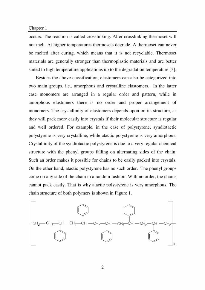
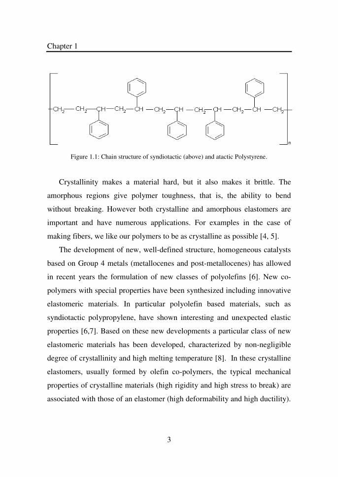
and well ordered. For example, in the case of polystyrene, syndiotactic

polystyrene is very crystalline, while atactic polystyrene is very amorphous.

Crystallinity of the syndiotactic polystyrene is due to a very regular chemical

structure with the phenyl groups falling on alternating sides of the chain.

Such an order makes it possible for chains to be easily packed into crystals.

On the other hand, atactic polystyrene has no such order. The phenyl groups

come on any side of the chain in a random fashion. With no order, the chains

cannot pack easily. That is why atactic polystyrene is very amorphous. The

chain structure of both polymers is shown in Figure 1.

Chapter 1

3

Figure 1.1: Chain structure of syndiotactic (above) and atactic Polystyrene.

Crystallinity makes a material hard, but it also makes it brittle. The

amorphous regions give polymer toughness, that is, the ability to bend

without breaking. However both crystalline and amorphous elastomers are

important and have numerous applications. For examples in the case of

making fibers, we like our polymers to be as crystalline as possible [4, 5].

The development of new, well-defined structure, homogeneous catalysts

based on Group 4 metals (metallocenes and post-metallocenes) has allowed

in recent years the formulation of new classes of polyolefins [6]. New co-

polymers with special properties have been synthesized including innovative

elastomeric materials. In particular polyolefin based materials, such as

syndiotactic polypropylene, have shown interesting and unexpected elastic

properties [6,7]. Based on these new developments a particular class of new

elastomeric materials has been developed, characterized by non-negligible

degree of crystallinity and high melting temperature [8]. In these crystalline

elastomers, usually formed by olefin co-polymers, the typical mechanical

properties of crystalline materials (high rigidity and high stress to break) are

associated with those of an elastomer (high deformability and high ductility).

Chapter 1

4

For these reasons, crystalline elastomers constitute a class of very promising

innovative materials for applications in different technological areas.

In the study of crystalline elastomers, a relevant area of research is

certainly that of the relationships between molecular architecture and

macroscopic properties. As it has been already pointed out, the use of very

selective catalysts allow for the synthesis of "tailored" polyolefins where

molecular characteristics such as stereoregularity, regioregularity,

distribution of defects, molecular mass and distribution of molecular masses

can be accurately. This, in turn, opens the way to the production of materials

whose ultimate and processing physical properties can be selectively

targeted.

In this area of research, the role of rheology can assume a crucial

relevance. Rheology has been always used as a qualitative and quantitative

tool in polymer science and engineering for many years. Areas such as

polymer processing and quality control have enjoyed the use of rheological

methodologies to determine the flow properties of polymer melts and more

complex polymer-based systems (e.g., blends, suspensions). More recently,

rheological techniques have been increasingly used as a tool to relate the

behavior of polymer systems under deformation and/or flow to the local

microstructure of the system at different length scales. In particular, the

development of rheological models on a molecular basis [70] has led to the

determination of relations (often quantitative) between the macroscopic

rheological properties and the molecular characteristics of the polymeric

chain (such as, for example, molecular weight, degree of branching,

entanglement density). For all these reasons, rheology can be seen as a

promising, successful instrument to help in a better understanding of the

Chapter 1

5

molecular architecture of crystalline elastomers and of the relations between

such architecture and the other macroscopic properties of these materials.

Based on the above, it can be said that rheology is expected to play a role

in achieving the rational design of materials based on tailored polyolefins.

Rheological techniques, in fact, are often more sensitive to certain aspects of

the molecular structure and easier to use than other more conventional

analytical techniques. The general aim of the present research work is to

explore the relationships between the rheological response and the molecular

structure of the class of innovative crystalline elastomers. Research

objectives of this research work are depicted below in detail.

1.2. Research Objectives

1. To explore the rheological behavior of selected poly-olefin based

crystalline elastomers in the melt state and to relate the rheological

response to the local architecture of the polymer chain.

2. To study the quiescent crystallization behavior of selected crystalline

elastomers by coupling rheological methods to more conventional

techniques (such as Differential Scanning Calorimetry) and to relate the

crystallization behavior to the stereo-regularity of the polymer chain.

3. To explore the role of extensional flow on the crystallization of

selected polyolefins and to relate such an effect to the molecular order

of the polymer chain.

First objective: We want to determine the rheological parameters of olefin

based crystalline elastomers in the melt state, in order to relate them to the

molecular architecture. For this we will need to choose and conduct suitable

rheological experiments. We will carry out all the rheological experiments

using linear, small amplitude shear oscillatory flow experiments. A general

Chapter 1

6

advantage of this method is that a single instrument can cover a wide range

of frequencies. The typical frequency range of the available rheometers is

0.001 to 500 rad/s. Different methods, such as the Time Temperature

Superposition (TTS) principle will be applied to explore the rheological

behavior of elastomer samples in order to uncover the higher frequency

range. As a second step, the relationship between melt rheological response

and molecular structure of the selected polymers will be explored. In fact, the

melt rheological properties are very sensitive to the molecular structure. For

example, the zero shear viscosity is used to detect the long chain branching.

Moreover, melt rheological data are very sensitive to Molecular Weight

(MW) and to Molecular Wight Distribution (MWD) [13]. In our case the

best candidate rheological quantity to be explored is the so-called “plateau

modulus”, to be obtained from linear viscoelastic data. This is an important

characteristic constant of each polymer, as it can be related to other

microstructure parameters using the classical reptation theories of polymer

chain dynamics [70]. Our aim will be to relate the plateau modulus to the

local degree of strereo-regularity of the polymer chain.

Second objective: In order to examine the quiescent crystallization behavior

of polyolefins of different stereoregularity by rheological technique two

different experimental techniques will be used (isothermal and non-

isothermal crystallization). Isothermal crystallization will be conducted by

fast cooling of a polymer melt from above its melting point temperature to

the crystallization temperature, TC and holding it at that temperature until

crystallization is completed. While in non-isothermal crystallization the

polymer melt will be cooled to the temperature below melting point by slow

cooling rates. The results obtained from rheological technique will be

compared with the differential scanning calorimetric (DSC) analysis.

Chapter 1

7

Third objective: In the extensional flow study the first objective is to

examine the crystallization kinetics by the application of extensional rate at a

temperature above the melting point. The first step is to heat the sample

above the melting point in order to break down all the crystals. After

annealing for shorter time, the sample will be cooled to a temperature

slightly above the melting point. The effect of extensional flow on

crystallization kinetics will be estimated on the basis of change in the

induction time due to extensional flow. The results will be verified by some

X-Ray analysis of the stretched samples.

After successfully achieving the first objective, effect of extensional flow

on the crystallization process will be examined by applying the extensional

rate at a temperature below melting point and above crystallization

temperature. The selection of temperature will be made by taking care of the

following two points. The temperature should not be in the range where

quiescent crystallization kinetics is faster. Because in this case it will not be

possible to see the effect of extensional rate on the kinetics of crystallization.

The temperature should also not be high to the extent that there is no effect

of extensional rate on the crystallization kinetics. The selected temperature at

which extensional rate will be applied should be in optimum region, where

one is able to analyze the effect of extensional rate on the kinetics of

crystallization.

1.3. Literature Review

The literature review section has been divided into five sections i.e.,

synthesis, mechanical properties, rheology, crystallization and flow induced

crystallization.

Chapter 1

8

1.3.1. Synthesis

Crystalline elastomers such as polypropylene, poly-1butene, syndiotactic

polystyrene and their co-polymers, are synthesized by the process of

polymerization. Polymerization is the process of combining many small

molecules known as monomers into a covalently bonded chain [14].

Different methods have been reported in literature [15-55]. Polymer samples

which will be used in this work are olefin based crystalline elastomers

synthesized by Co-ordination polymerization (Ziegler Natta catalysis and

Metallocene methods). Therefore the main focus of this section will be on

co-ordination methods used for the synthesis of the olefin based crystalline

elastomers. Synthesis methods used so far for these polymers can be

categorized into four methods: ionic polymerization,cationic polymerization,

free radical polymerization and co-ordination polymerization.

Ionic polymerization occurs by the formation of the carbanion ion.

Formation of the carbanion ion occurs by the attack of a nucleophilic reagent

at one end of the double bond [16-18]. This first step, formation of the

carbanion ion is called the initiation step. For example, in the case of

ethylene.

Figure 1.2: Chain Initiation step of Ionic polymerization.

Attacking of carbanion ion on another alkene molecule would give a four

carbon-carbon anion and subsequent additions to further alkene molecules

would lead to a higher molecular weight chain. This second step is called the

chain propagation step.

Chapter 1

9

Figure1.3: Chain Propagation step of Ionic polymerization.

The third and last step during the anionic polymerization is the chain

terminating step. The termination of polymerization will occur by

terminating the carbanion ion. The ion can be terminated by the addition of

the proton. The shortcoming and drawback of this process is that, in this

process, large number of powerful electron attracting groups are required to

speed up the nucleophilic attack.

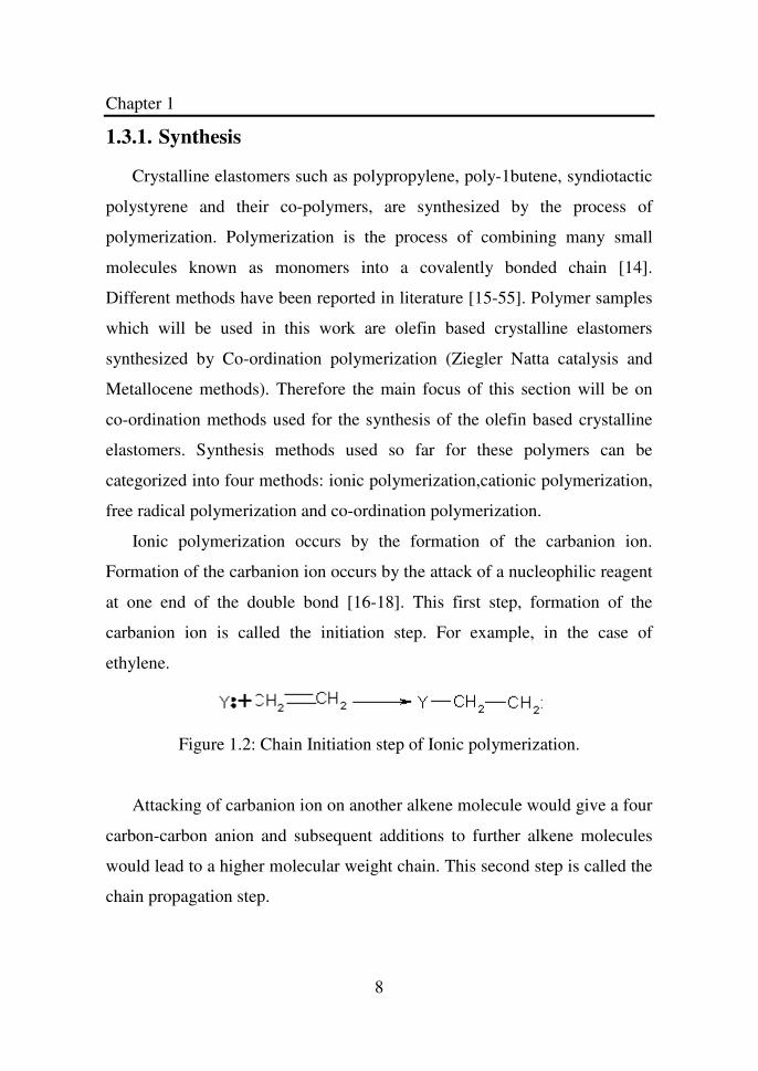
In cationic polymerization, formation of the carbonium carbon occurs. This

occurs by the addition of the proton to alkene from acid (suitable acid).

Then, in the absence of strong nucleophilic reagents, another alkene

molecule donates an electron pair and forms a longer chain cation [19].

Figure 1.4: Reaction mechanism of Cationic polymerization process.

In free radical polymerization, formation of free radicals occurs (initiation).

Then subsequent addition of radicals to the alkene molecules occurs

(propagation). The chain termination step may occur by any reaction

resulting in combination or disproportionation of free radicals [19].

In all the above different methods, special nucleophilic reagents and

other reaction conditions are required. All the above methods have been

Chapter 1

10

replaced by the Zeigler Natta catalysis, metallocene and post metallocene

methods, generally known as co-ordination polymerization methods [20-55].

Co-ordination polymerization is the process of polymerization in the

presence of a catalyst. Ziegler introduced a new type of catalyst in 1940

(alkane solvent containing a suspension of the insoluble reaction product

from triethylealuminium and titanium tetrachloride). The Ziegler process can

produce an efficient and high molecular weight with remarkable physical

properties. The usual characteristics of these reactions indicate that no simple

anion, cation or free radical mechanisms are involved [20-55].

Generally this type of polymerization occurs in the three steps: (i)

Initiation (ii) Propagation and (iii) Termination. The mechanism of this type

of chemical reaction has been explained very well by the Cossee model [22].

According to this model during the initiation step co-ordination occurs,

where co-ordination occurs between the metal and the alkene monomer.

Figure 1.5: Chain initiation step during the Co-ordination polymerization process.

In the second step the co-ordination proceeds to another state called transition state..

Figure 1.6: Transition state during the Co-ordination polymerization process.

The third step is the insertion of alkene monomer.

Chapter 1

11

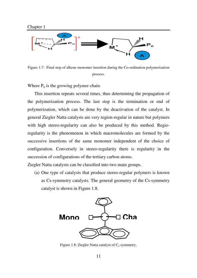
Figure 1.7: Final step of alkene monomer insertion during the Co-ordination polymerization

process.

Where Pn is the growing polymer chain.

This insertion repeats several times, thus determining the propagation of

the polymerization process. The last step is the termination or end of

polymerization, which can be done by the deactivation of the catalyst. In

general Ziegler Natta catalysts are very region-regular in nature but polymers

with high stereo-regularity can also be produced by this method. Regio-

regularity is the phenomenon in which macromolecules are formed by the

successive insertions of the same monomer independent of the choice of

configuration. Conversely in stereo-regularity there is regularity in the

succession of configurations of the tertiary carbon atoms.

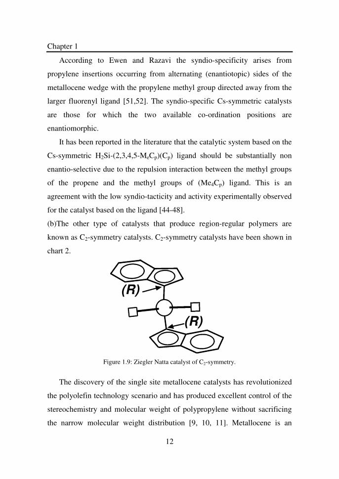
Ziegler Natta catalysts can be classified into two main groups.

(a) One type of catalysts that produce stereo-regular polymers is known

as Cs-symmetry catalysts. The general geometry of the Cs-symmetry

catalyst is shown in Figure 1.8.

Figure 1.8: Ziegler Natta catalyst of Cs-symmetry.

Mono Cha

Chapter 1

12

According to Ewen and Razavi the syndio-specificity arises from

propylene insertions occurring from alternating (enantiotopic) sides of the

metallocene wedge with the propylene methyl group directed away from the

larger fluorenyl ligand [51,52]. The syndio-specific Cs-symmetric catalysts

are those for which the two available co-ordination positions are

enantiomorphic.

It has been reported in the literature that the catalytic system based on the

Cs-symmetric H2Si-(2,3,4,5-MeCp)(Cp) ligand should be substantially non

enantio-selective due to the repulsion interaction between the methyl groups

of the propene and the methyl groups of (Me4Cp) ligand. This is an

agreement with the low syndio-tacticity and activity experimentally observed

for the catalyst based on the ligand [44-48].

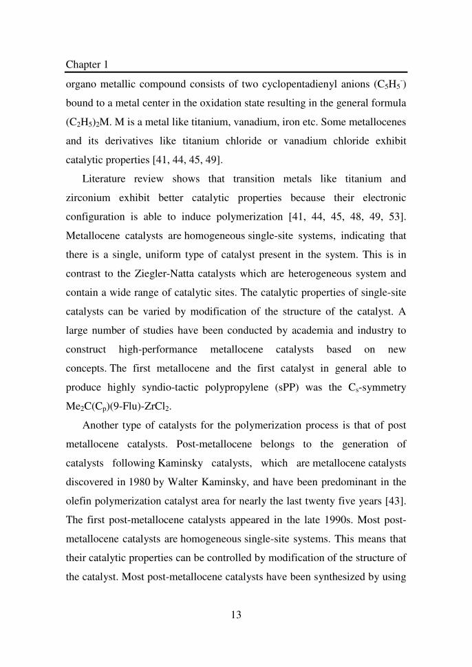
(b)The other type of catalysts that produce region-regular polymers are

known as C2-symmetry catalysts. C2-symmetry catalysts have been shown in

chart 2.

Figure 1.9: Ziegler Natta catalyst of C2-symmetry.

The discovery of the single site metallocene catalysts has revolutionized

the polyolefin technology scenario and has produced excellent control of the

stereochemistry and molecular weight of polypropylene without sacrificing

the narrow molecular weight distribution [9, 10, 11]. Metallocene is an

(R)

(R)

Chapter 1

13

organo metallic compound consists of two cyclopentadienyl anions (C5H5-)

bound to a metal center in the oxidation state resulting in the general formula

(C2H5)2M. M is a metal like titanium, vanadium, iron etc. Some metallocenes

and its derivatives like titanium chloride or vanadium chloride exhibit

catalytic properties [41, 44, 45, 49].

Literature review shows that transition metals like titanium and

zirconium exhibit better catalytic properties because their electronic

configuration is able to induce polymerization [41, 44, 45, 48, 49, 53].

Metallocene catalysts are homogeneous single-site systems, indicating that

there is a single, uniform type of catalyst present in the system. This is in

contrast to the Ziegler-Natta catalysts which are heterogeneous system and

contain a wide range of catalytic sites. The catalytic properties of single-site

catalysts can be varied by modification of the structure of the catalyst. A

large number of studies have been conducted by academia and industry to

construct high-performance metallocene catalysts based on new

concepts. The first metallocene and the first catalyst in general able to

produce highly syndio-tactic polypropylene (sPP) was the Cs-symmetry

Me2C(Cp)(9-Flu)-ZrCl2.

Another type of catalysts for the polymerization process is that of post

metallocene catalysts. Post-metallocene belongs to the generation of

catalysts following Kaminsky catalysts, which are metallocene catalysts

discovered in 1980 by Walter Kaminsky, and have been predominant in the

olefin polymerization catalyst area for nearly the last twenty five years [43].

The first post-metallocene catalysts appeared in the late 1990s. Most post-

metallocene catalysts are homogeneous single-site systems. This means that

their catalytic properties can be controlled by modification of the structure of

the catalyst. Most post-metallocene catalysts have been synthesized by using

Chapter 1

14

early transition metals. However, late transition metal complexes such as

nickel, palladium, and iron complexes have also been reported as good

catalysts for olefin polymerization. These different techniques of the co-

ordination polymerization have been explored by many researchers [26, 27,

28, 37, 40].

Eckstein et al. [86] have followed out research on the synthesis and

rheological properties of polypropylene melts. Atactic polypropylene was

synthesized using methylalumoxane (MAO) at 283 K in a mixture of liquid

propene and toluene. Polymerization was executed in a 1.6 L Buechi glass

autoclave reactor equipped with a torsion valve. During the polymerization

process, the temperature was kept constant at 283 K by a combination of

inner and outer cooling.

One way of improving or changing the properties of the polymers is to

use co-monomer. A co-monomer is used in commercial polymers to alter the

properties of a base polymer, for example to change its glass transition

temperature, degree of crystallinity or swelling behavior, or to make it more

compatible with a plasticizer or dye or to enhance its stability. The process

which is used for its synthesis is called co-polymerization. When

polymerization occurs in a mixture of monomers, there will be some

competition between the different kinds of monomers to add to the growing

chain and produce the polymer chain. The rates of incorporation of various

monomers into the growing free radical chains have been studied in

considerable detail. These rates depend markedly on the nature of the

monomer being added and of the character of the radical at the end of the

chain. The co-polymerization processes can be classified into the three types

depending on the values of the monomer reactivity ratios [55, 56].

1. When the product of the two monomer reactivity ratios is unity.

Chapter 1

15

2. When the product of the two monomer reactivity ratios is less than

unity.

3. When the product of the two monomer reactivity ratios is greater than

unity.

Ideal co-polymerization occurs in a case when both the propagating

species show the same preference.

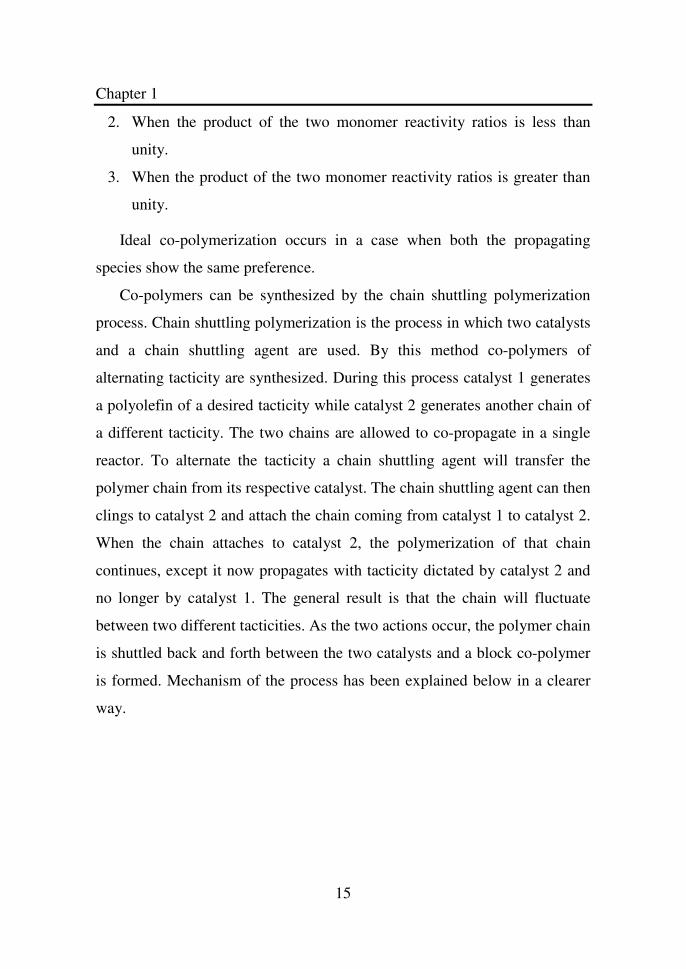
Co-polymers can be synthesized by the chain shuttling polymerization

process. Chain shuttling polymerization is the process in which two catalysts

and a chain shuttling agent are used. By this method co-polymers of

alternating tacticity are synthesized. During this process catalyst 1 generates

a polyolefin of a desired tacticity while catalyst 2 generates another chain of

a different tacticity. The two chains are allowed to co-propagate in a single

reactor. To alternate the tacticity a chain shuttling agent will transfer the

polymer chain from its respective catalyst. The chain shuttling agent can then

clings to catalyst 2 and attach the chain coming from catalyst 1 to catalyst 2.

When the chain attaches to catalyst 2, the polymerization of that chain

continues, except it now propagates with tacticity dictated by catalyst 2 and

no longer by catalyst 1. The general result is that the chain will fluctuate

between two different tacticities. As the two actions occur, the polymer chain

is shuttled back and forth between the two catalysts and a block co-polymer

is formed. Mechanism of the process has been explained below in a clearer

way.

Chapter 1

16

Figure 1.10: Mechanism of Chain shuttling polymerization process.

Where A, B and X are catalyst 1, catalyst 2 and chain shuttling agent

respectively. and ------ are chain 1 and chain 2 respectively.

1.3.2. Mechanical Properties

Several research works have been reported in the literature not only on

the synthesis, but also on the mechanical and rheological properties of

polyolefin polymers and co-polymers. As a way of example, Wang et al.

[10], have examined the synthesis, dynamic mechanical and rheological

properties of the long chain branched ethylene/propylene co-polymers. The

novel series of long chain branched ethylene/propylene copolymers were

synthesized with a constrained geometry catalyst (CGC), [C5Me4

(SiMe2NtBu)] TiMe2, and had various propylene molar fractions of 0.01-0.11

and long chain branch frequencies (LCBF) of 0.05-0.22. The linear

ethylene/propylene co-polymers were synthesized with an ansa-zirconocene

catalyst, rac-Et (Ind)2ZrCl2 (EBI), and contained similar levels of propylene

incorporation as the CGC copolymers, but no long chain branched. Wang et

al. showed that catalyst system, reaction conditions and synthesis technique

affect the mechanical, thermal and rheological properties of the polymer

Chapter 1

17

synthesized. In this section, attention will be given to the mechanical

properties of crystalline elastomers.

Characteristics of polymers like stereoregularity, molecular mass and

polydispersity depend upon on the catalyst system and reaction conditions of

the polymerization process. These characteristics are the main structural

factors, which affect the physical and mechanical properties. Mechanical

properties of polyolefins are largely related to the crystal structure and

morphology, which in turn depend on the chain microstructure generated by

the catalyst system used [58, 59].

The mechanical properties of the crystalline polymers strongly depend

upon on the stereo-regularity and initial morphology of the samples [59-64].

Unoriented samples of high stereo-regularity and crystalline syndiotactic

polypropylene behave as a typical crystalline thermoplastic material showing

plastic deformation via necking during stretching with high values of

Young’s modulus [57-60]. The samples experience a partial elastic recovery

after breaking or upon releasing the tension after deformation [59-65]. On

the other hand oriented fibers of syndiotactic polypropylene exhibit a perfect

elastic behavior upon successive stretching and relaxation cycles [60-65].

Strength and toughness are the two main mechanical properties of the

polymers. Strength is a mechanical property, which gives us information that

how much a material is strong [66]. In the other words strength can also be

defined as the stress needed to break the sample. In stress-strain experiments,

a polymer sample is subjected to a constant elongation rate, and stress is

measured as a function of time. Generally the polymer sample, which may be

in the form of circular in cross-section or rectangular, is molded. It is

clamped at both ends and pulled at one of the clamped ends (normally in

downward direction) at constant elongation. The shape of the test sample is

Chapter 1

18

designed to encourage failure at the thinner middle portion. The load or

stress is determined at the fixed end by means of a load transducer as a

function of the elongation, which is measured by means of mechanical,

optical or electronic strain gauges. The experimental data are generally noted

as engineering (nominal) stress (σ) vs. engineering (nominal) strain. The

engineering stress is defined as:

= / (1.1)

Where σ = stress, F= Force and A= area.

When a material is subjected to stress, there are two possibilities. It will

deform and will come back to its initial shape and dimensions after the

removal of the stress or it will deform permanently. This ability of deformed

material to recover to its original dimensions is known as elastic behavior.

Beyond the limit of elastic behavior (elastic limit), a material will experience

a permanent change or deformation even when the load is removed. Such a

material is known to have undergone plastic deformation. For most

materials, Hooke’s law is obeyed within the elastic limit, that is stress

proportional to strain. However proportionality between stress and strain

does not always hold when a material shows elastic behavior. A typical

example is rubber, which is elastic but does not exhibit Hookean behavior

over the entire elastic region.

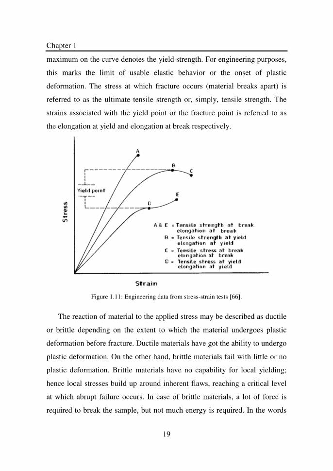
Figure 1.11 dictates mechanical properties that are obtainable from

stress-strain experiments. The slope of the initial linear portion of the curve,

within which Hooke’s law is obeyed, gives the elastic or Young’s modulus.

The determination of the elastic limit is tough and is dependent on the

sensitivity of the strain-measuring devices employed. Consequently, it is

common practice to replace it with the proportional limit, which defines the

point where the non-linear response is noted on the stress-strain curve. The

Chapter 1

19

maximum on the curve denotes the yield strength. For engineering purposes,

this marks the limit of usable elastic behavior or the onset of plastic

deformation. The stress at which fracture occurs (material breaks apart) is

referred to as the ultimate tensile strength or, simply, tensile strength. The

strains associated with the yield point or the fracture point is referred to as

the elongation at yield and elongation at break respectively.

Figure 1.11: Engineering data from stress-strain tests [66].

The reaction of material to the applied stress may be described as ductile

or brittle depending on the extent to which the material undergoes plastic

deformation before fracture. Ductile materials have got the ability to undergo

plastic deformation. On the other hand, brittle materials fail with little or no

plastic deformation. Brittle materials have no capability for local yielding;

hence local stresses build up around inherent flaws, reaching a critical level

at which abrupt failure occurs. In case of brittle materials, a lot of force is

required to break the sample, but not much energy is required. In the words

Chapter 1

20

brittle materials have high strength and low toughness. Toughness of

materials tells us that how much energy is required to break the sample.

Therefore it is not necessary that a material will be strong as well as tough.

While in the case of ductile materials, toughness is higher than the strength.

Because in case of ductile material, it deforms a lot before breaking.

Deformation allows a sample to dissipate energy. If a sample cannot deform,

the energy would not be dissipated and will cause the sample to break.

Moving to the class of materials of specific interest for the present work,

several studies have been considered the solid mechanical behavior of

polyolefin crystalline elastomer and their relations with the stereo-regularity

of their molecular architecture. Auriemma et al. conducted research on the

mechanical properties and structure of syndiotactic polypropylene samples in

order to clarify the origin of its elastic behavior [67]. They analyzed the

mechanical properties of syndiotactic polypropylene samples having

different degrees of tacticity. They found that the elastic properties of the

syndiotactic polypropylene mainly originate from a reversible crystal-crystal

phase transition, which occurs during the stretching and when the tension is

removed. They found that conformational crystal-crystal transitions are

responsible for the elastic behavior of the syndiotactic polypropylene. They

also found that, in the less stereo-regular samples, there is a plastic and

permanent deformation and elastic properties are suppressed. The reason of

this behavior is the absence of crystal-crystal transition in poorly syndiotactic

polypropylene samples. They also examined the mechanical properties

(Young’s modulus, stress and strain at break, tension and elastic recovery at

a given elongation) of the samples. In their analysis they used two types of

syndiotactic polypropylene samples i.e., unoriented compression molded

samples and strained and stress relaxed syndiotactic polypropylene samples

Chapter 1

21

(oriented samples). The latter were obtained by keeping syndiotactic

polypropylene fiber samples under tension for two days and then removing

the stress, thus allowing for fiber relaxation. Syndiotactic polypropylene

samples were compressed and stretched up to a given strain of 400% and

600%. They concluded that the elastic properties of the unoriented samples

are poor since they undergo a plastic deformation by stretching and do not

present any recovery of the initial dimensions upon release of the tension.

Similar behavior was observed for the less stereo-regular syndiotactic

polypropylene samples. Conversely, the mechanical properties of the

oriented stress relaxed fibers were found similar to the mechanical properties

of true elastomers. For these samples of syndiotactic polypropylene the

stress-strain curve were found to be almost linear.

In another work De Rosa et al., found almost the same mechanical

properties during their investigation on the isotactic polypropylene samples.

They found that poor stereo-regular samples showed remarkable strain

hardening due to the low plastic resistance of crystals and by straightening of

the entangled network. They also concluded that the different mechanical

behavior is due to the structural transformations that occur during stretching

[59].

More recently Auriemma et al. [68] confirmed the observed behavior for

different types of stereo-block polypropylenes. In particular, unoriented

samples have a stress-strain curve typical of thermoplastic material with a

partial but significant recovery of the initial dimensions measured after

breaking and after releasing the tension from different degrees of

deformation. On the other hand, stress relaxed fibers were found to show

tensile properties typical of thermoplastic elastomers with high values of

Chapter 1

22

elongation before breaking, tensile strength and Young’s modulus and

showed strong strain hardening at high values of deformation [68].

In conclusion, it can be said that the mechanical properties of polyolefin

based crystalline polymers are affected by the stereo- and region-regularity

of the polymer chain. These properties determine both the formation and the

type of the crystalline phase, which is also strongly affected by the

mechanical history. In turn, all these phenomena are found to have a

profound influence on the mechanical properties of the solid materials.

1.3.3. Rheology

Rheology has a key role in polymer research being an important link to

the chain of knowledge. Polymers such as elastomers are viscoelastic in the

melt, which means that they possess both a viscous and an elastic component

[69-85]. In this section we will focus only on aspects of the rheological

behavior that are of interest for this work. In particular, attention will be

given to the so-called linear viscoelasticity.

One of the central objectives of rheology is the determination of the so-

called constitutive equation of the material. A constitutive equation is a

mathematical relation that links the tensional state (the stress tensor) to the

deformation history applied to the material. The study of the rheological

behavior of viscoelastic materials and in particular of polymer melts has

been tipically conducted along two different lines. On the one hand the

“continuum mechanics” approach starts from the phenomenological

observation of the material response under deformation and/or flow. From

there, a mechanical description of the material as mathematical “continuum”

is derived without making assumptions on the particular microscopic

structure of the system. Constitutive equations are then obtained that are

consistent with the observed behavior, while satisfying at the same some

Chapter 1

23

more general constraints (such as thermodynamic consistency). One positive

aspect of the continuum mechanics approach is that the (often semi-

empirical) constitutive equations possess a relative level of mathematical

flexibility, thus allowing for successive refinements of the model in order to

improve the agreement between theory and experimental observations.

Another, completely different approach is the so-called “molecular” or

“micro-rheology” modeling. In this case constitutive equations are built on

the basis of a microscopic description of the material microstructure. In the

case of polymer melts, in particular, a physical model for the single polymer

chain and for entangled chain network is required. Polymer chains are

Brownian objects. Therefore the material macroscopic behavior can be

derived only by introducing the mathematical description of the polymer

chain into the classical equation of statistical thermodynamics. Following

these lines, rheological constitutive equations can be derived. The main

difficulty of this approach is in its generally very complex mathematical

formulation. On the other hand, micro-rheology modeling allows

establishing direct relations between the local details of the molecular

structure and the observable rheological properties.

In the following, some basic information on constitutive equations and

on micro-rheological models, which will be relevant for the subsequent

development of this work will be given. [2].

1.3.3.1. Continuum mechanics linear viscoelasticity

As it was said before, in continuum mechanics, constitutive equations are

developed on the basis of the observed phenomenological behavior of the

material. When considering viscoelastic fluids, that are materials that exhibit

both a viscous and elastic materials, it is useful to start from the so-called

linear viscoelasticity hypothesis. Linear viscoelasticity implies that the

Chapter 1

24

response (e.g. strain) of the fluid at any time is directly proportional to the

value of the initiating signal (e.g. stress). So for example, doubling the stress

will double the strain. Starting from this hypothesis it is possible to develop

linear constitutive equations that relate the state of stress in the fluid to the

corresponding deformation history. By referring for simplicity to a single

component of the stress tensor (e.g.,the shear stress) and to the corresponding

deformation (the shear deformation), a general differential constitutive

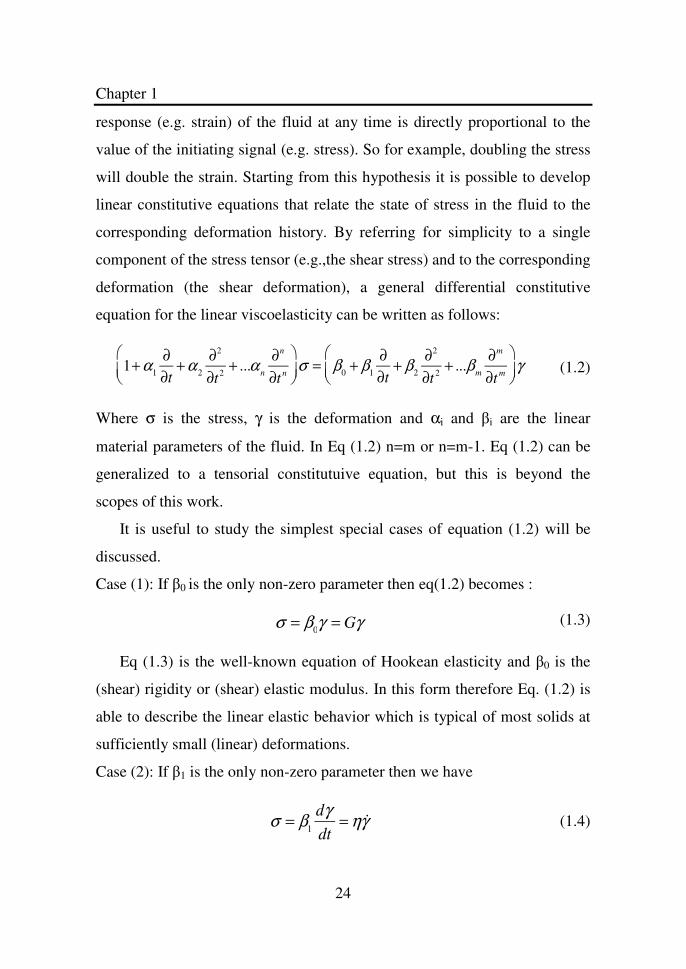
equation for the linear viscoelasticity can be written as follows:

1+ α1

∂

∂t+ α 2

∂2

∂t2

+ ...αn

∂n

∂tn

σ = β0 + β1

∂

∂t+ β2

∂2

∂t2

+ ...βm

∂m

∂tm

γ

(1.2)

Where σ is the stress, γ is the deformation and αi and βi are the linear

material parameters of the fluid. In Eq (1.2) n=m or n=m-1. Eq (1.2) can be

generalized to a tensorial constitutuive equation, but this is beyond the

scopes of this work.

It is useful to study the simplest special cases of equation (1.2) will be

discussed.

Case (1): If β0 is the only non-zero parameter then eq(1.2) becomes :

σ = β0γ = Gγ (1.3)

Eq (1.3) is the well-known equation of Hookean elasticity and β0 is the

(shear) rigidity or (shear) elastic modulus. In this form therefore Eq. (1.2) is

able to describe the linear elastic behavior which is typical of most solids at

sufficiently small (linear) deformations.

Case (2): If β1 is the only non-zero parameter then we have

σ = β1

dγ

dt= η &γ

(1.4)

Chapter 1

25

Eq(1.4) is the Newton law of viscosity. Here β1 is the fluid viscosity. Eqs

(1.3) and (1.4) are particularly relevant as they define the simplest types of

linear behavior corresponding to the linear elastic solid and to the linear

viscous (Newtonian liquid). A material that exhibits both characteristics will

be indeed viscoelastic.

Case (3): If β0 and β1 are the only non-zero parameters, then we have

σ = β1

dγ

dt+ β0 = η &γ + Gγ

(1.5)

ηγγσ += G (1.6)

This is one of the simplest models of viscoelasticity, which is known as

Kelvin-Voigt model. The Kelvin model describes sufficiently well the

viscoelastic behavior of a solid material. In fact, under steady state

conditions, the material obeys the linear elasticity law.

Case (4): If α1 and β1 are the only non-zero parameters then we have:

σ + τ

dσ

dt= η &γ

(1.7)

Eq (1.7) is universally known as the Maxwell model. Here α1=τ is the so-

called relaxation time. Eq (1.7) is the simplest constitutive continuum

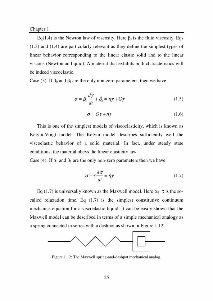
mechanics equation for a viscoelastic liquid. It can be easily shown that the

Maxwell model can be described in terms of a simple mechanical analogy as

a spring connected in series with a dashpot as shown in Figure 1.12.

Figure 1.12: The Maxwell spring-and-dashpot mechanical analog.

Chapter 1

26

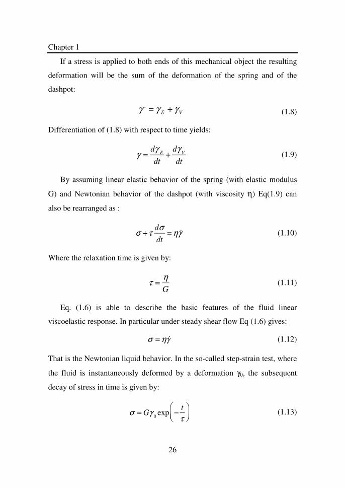
If a stress is applied to both ends of this mechanical object the resulting

deformation will be the sum of the deformation of the spring and of the

dashpot:

VE γγγ +=.

(1.8)

Differentiation of (1.8) with respect to time yields:

γ =

dγE

dt+

dγV

dt

(1.9)

By assuming linear elastic behavior of the spring (with elastic modulus

G) and Newtonian behavior of the dashpot (with viscosity η) Eq(1.9) can

also be rearranged as :

σ + τ

dσ

dt= η &γ

(1.10)

Where the relaxation time is given by:

τ =

η

G

(1.11)

Eq. (1.6) is able to describe the basic features of the fluid linear

viscoelastic response. In particular under steady shear flow Eq (1.6) gives:

σ = η &γ (1.12)

That is the Newtonian liquid behavior. In the so-called step-strain test, where

the fluid is instantaneously deformed by a deformation γ0, the subsequent

decay of stress in time is given by:

σ = Gγ

0exp −

t

τ

(1.13)

Chapter 1

27

Where it is clear the meaning of the relaxation time of the material.

Of particular interest is the response of a Maxwell viscoelastic fluid to

periodic oscillatory shear flow. It can be easily shown that if the fluid is

subjected to a sinusoidal deformation of amplitude γ0 and frequency ω:

γ = γ 0 sin ωt( ) (1.14)

Under linear condition the resulting stress response will be:

σ = σ 0 sin ωt +δ( ) (1.15)

The phase angle (or delay) δ gives a direct indication of the viscoelastic

nature of the fluid. If δ=0°, the stress is in phase with the deformation, and

the behavior is that of an elastic solid. If δ=90° the stress will be in phase

with the deformation rate:

&γ = γ 0ω cos ωt( ) (1.16)

and the observed behavior will that of a purely Newtonian fluid. When

0°<δ<90°, both elastic and viscous components will be present.

The linear oscillatory viscoelastic response of the Maxwell fluid can be

recast in the following form:

σ

γ 0

= ′G sinω t + ′′G cosω t

(1.17)

where G` and G`` are the so-called elastic (or conservative) and viscous

(dissipative) moduli, as they are a measure of the two different component of

the material viscoelastic response. For the Maxwell model one has:

Chapter 1

28

( )( )

( )

( )( )

2

2

2

1

=1

G G

G G

τωω

τω

τωω

τω

′ =+

′′+

(1.18)

Eq. (1.18) shows the basic features of G`and G``. When ω<<τ, the

dissipative modulus is always larger than elastic modulus (both going to zero

for vanishingly frequencies) and they obey the following scaling laws:

′G ∝ω 2

′′G ∝ω

(1.19)

When ω<<τ, G`` goes to zero, where as G` goes to a plateau which

correspond to the elastic modulus (G`) of the Maxwell model. It will be

shown later that the plateau modulus of a polymer is a fundamental

parameter to describe the chain molecular structure. For ω=1/τ the G``

reaches a maximum which correspond also to the value where the two

moduli cross-over. For this reason 1/τ is also called the cross-over frequency,

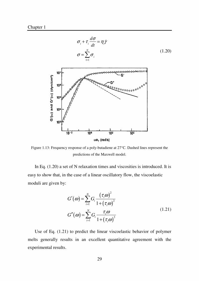
ωco. A typical plot of the frequency response of the two moduli for a polymer

obeying the Maxwell model (at least for not too high frequencies) is given in

Figure 1.13.

As said before, the Maxwell model gives a qualitative good description

of the linear viscoelastic behavior, in particular as far as the frequency

response is concerned. Quantitative agreement however requires more

complex models. One simple extension of the Maxwell model, which allows

for good quantitative predictions of the frequency response of polymer melts

is to allow for the presence of more than one relaxation time. This multi-

mode Maxwell model is represented by the following equations:

Chapter 1

29

σi+ τ

i

dσ

dt= η

i&γ

σ = σi

1=1

N

∑

(1.20)

Figure 1.13: Frequency response of a poly-butadiene at 27°C. Dashed lines represent the

predictions of the Maxwell model.

In Eq. (1.20) a set of N relaxation times and viscosities is introduced. It is

easy to show that, in the case of a linear oscillatory flow, the viscoelastic

moduli are given by:

( )( )

( )

( )( )

2

21

21

1

1

Ni

i

i i

Ni

i

i i

G G

G G

τ ωω

τ ω

τ ωω

τ ω

=

=

′ =+

′′ =+

∑

∑

(1.21)

Use of Eq. (1.21) to predict the linear viscoelastic behavior of polymer

melts generally results in an excellent quantitative agreement with the

experimental results.

Chapter 1

30

1.3.3.2. Micro-rheological modes

The continuum mechanics approach does not consider the microscopic

nature of the fluid. It only defines relations between stress and deformation

history on the basis of a purely phenomenological macroscopic approach.

Micro-rheology and molecular dynamics on the contrary are based on a

description of the fluid microstructure. Here we refer to the situation of melts

composed of linear polymer chains as it is the case for the polyolefins that

are the subject of the present study.

The starting point of a micro-rheological description of polymer melts

must recognize that the most important factor determining the dynamic

behavior of a polymer chain is its very large length compared to its lateral

dimension. Furthermore due to the very large number of internal degrees of

freedom, polymer chains are able to assume many different conformations.

As a consequence a single chain can be seen somewhat as a “thread”.

Alternatively, the chain can be seen as a broken line composed of N

monomers, each one of length b. In both cases, the shape and size of the

chain continuously change due to thermal agitation. Brownian motion, in

other words is able to incessantly alter the “conformation” of the chain,

which will explore different configurations. An example of possible

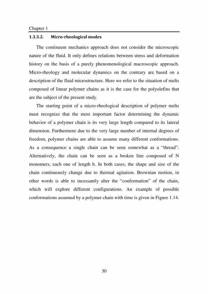
conformations assumed by a polymer chain with time is given in Figure 1.14.

Chapter 1

31

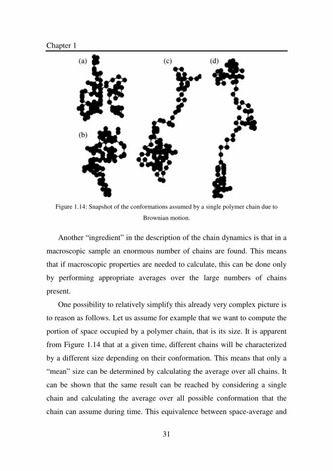
Figure 1.14: Snapshot of the conformations assumed by a single polymer chain due to

Brownian motion.

Another “ingredient” in the description of the chain dynamics is that in a

macroscopic sample an enormous number of chains are found. This means

that if macroscopic properties are needed to calculate, this can be done only

by performing appropriate averages over the large numbers of chains

present.

One possibility to relatively simplify this already very complex picture is

to reason as follows. Let us assume for example that we want to compute the

portion of space occupied by a polymer chain, that is its size. It is apparent

from Figure 1.14 that at a given time, different chains will be characterized

by a different size depending on their conformation. This means that only a

“mean” size can be determined by calculating the average over all chains. It

can be shown that the same result can be reached by considering a single

chain and calculating the average over all possible conformation that the

chain can assume during time. This equivalence between space-average and

Chapter 1

32

time-average is the so-called “ergodic principle”, which is at the basis of

statistical thermodynamics. In particular, it can be shown that under

quiescent conditions (that is in the absence of flow that can perturb the chain

conformation distribution) the average chain size is represented by the square

root of the so-called end-to-end mean square radius:

R2 = Nb2 (1.22)

R, as indicate by its name represents an average value of distance separating

the beginning and the end of the polymer chain. Since the number of

segments in the chain is directly proportional to its molecular weight. Eq

(1.22) informs that the average chain size scales with the square root of the

molecular weight.

The large number of conformation that can be assumed by a polymer

chain is also responsible for its elastic component. Let as assume to pick the

two ends of the chain and pull them in opposite directions, thus applying a

force (tension) along the chain. Under the action of the force, the chain will

uncoil, assuming an elongated conformation. When the force is released,

Brownian motion will induce a retraction of the chain, in the sense that, all

conformation becoming again available, the average size of the chain will

tend to the unperturbed, equilibrium value given by Eq. (1.22). It is clear that

thermal agitation plays the equivalent role of a spring-like restoring force.

This “entropic elasticity” (that is, an elasticity that is related to the degree of

conformational order of the chain) is at the basis of the elastic behavior of

polymeric liquids.

The situation depicted above becomes much more complex when a

polymer melt is considered. Here, many chains are present and interact with

each other. The main additional ingredient in this picture is that the motion

Chapter 1

33

of the chains (and therefore their conformational changes) is strongly

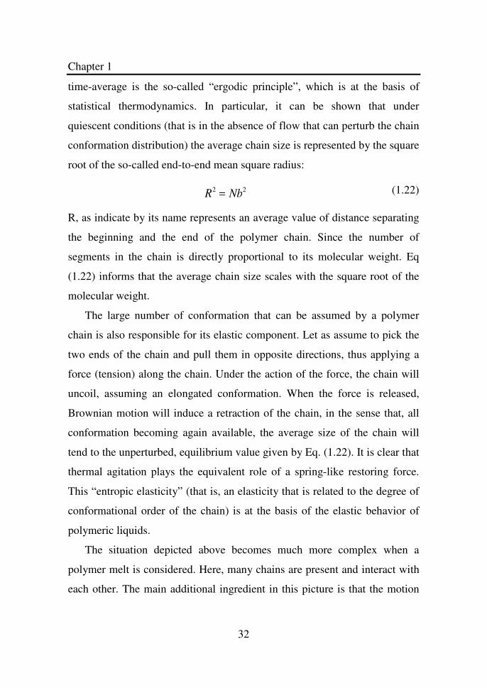
restricted by the presence of the other chains (see Figure 1.15).

Figure 1.15: A schematic view of the entangled melt.

Chains in fact cannot physically cross each other. The steric hindrance

between one chain and the others is universally known with the term

“entanglement”. The network of entangled chains determines an additional

elastic component on top of the entropic elasticity of the single chain.

Numerous research works have been reported in the literature on the

dynamics of chains in polymer melts [60-73]. Here, specific attention will be

given to one molecular or micro-rheological model, which is called the

reptation model. It will be shown that from this model we can extract

relations between rheological properties such as moduli, relaxation times,

and microstructural properties such as molecular weight, molecular weight

between entanglements and ultimately the chain molecular architecture.

According to the reptation model, the topological resistances imposed by

the neighboring chains on a given polymer chain restrict its motion to a tube

like region called the confining tube. A schematic view of this conceptual

idea is given in Figure 1.16.

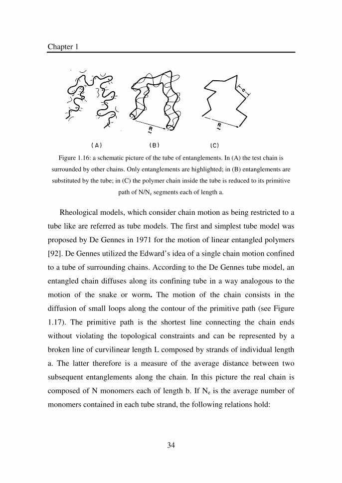
Chapter 1

34

Figure 1.16: a schematic picture of the tube of entanglements. In (A) the test chain is

surrounded by other chains. Only entanglements are highlighted; in (B) entanglements are

substituted by the tube; in (C) the polymer chain inside the tube is reduced to its primitive

path of N/Ne segments each of length a.

Rheological models, which consider chain motion as being restricted to a

tube like are referred as tube models. The first and simplest tube model was

proposed by De Gennes in 1971 for the motion of linear entangled polymers

[92]. De Gennes utilized the Edward’s idea of a single chain motion confined

to a tube of surrounding chains. According to the De Gennes tube model, an

entangled chain diffuses along its confining tube in a way analogous to the

motion of the snake or worm. The motion of the chain consists in the

diffusion of small loops along the contour of the primitive path (see Figure

1.17). The primitive path is the shortest line connecting the chain ends

without violating the topological constraints and can be represented by a

broken line of curvilinear length L composed by strands of individual length

a. The latter therefore is a measure of the average distance between two

subsequent entanglements along the chain. In this picture the real chain is

composed of N monomers each of length b. If Ne is the average number of

monomers contained in each tube strand, the following relations hold:

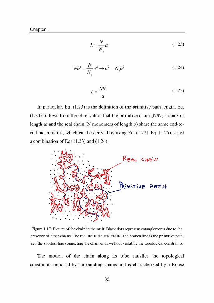
Chapter 1

35

L =N

Ne

a

(1.23)

Nb

2 =N

Ne

a2 → a

2 = Neb

2

(1.24)

L =

Nb2

a

(1.25)

In particular, Eq. (1.23) is the definition of the primitive path length. Eq.

(1.24) follows from the observation that the primitive chain (N/Ne strands of

length a) and the real chain (N monomers of length b) share the same end-to-

end mean radius, which can be derived by using Eq. (1.22). Eq. (1.25) is just

a combination of Eqs (1.23) and (1.24).

Figure 1.17: Picture of the chain in the melt. Black dots represent entanglements due to the

presence of other chains. The red line is the real chain. The broken line is the primitive path,

i.e., the shortest line connecting the chain ends without violating the topological constraints.

The motion of the chain along its tube satisfies the topological

constraints imposed by surrounding chains and is characterized by a Rouse

Chapter 1

36

friction coefficient Nζ, where ζ is the monomer friction coefficient. The

chain diffusion coefficient Dc which describes the Brownian motion of the

chain along its tube is simply the Rouse diffusion coefficient of the chain.

According to the Einstein’s relation it is given by:

Dc

=kT

Nζ

(1.26)

where k is the Boltzmann constant and T the absolute temperature. Due to

the presence of the entanglements, the only way for the chain to “escape”

from the tube of constraints is to diffuse along its backbone in reptation-like

style. This means that the time taken by the chain to diffuse out of the

original tube of length L will be given by:

T

rep=

L2

Dc

=ζb

2N

3

kTNe

=ζ b

2N

e

2

kT

N

Ne

3

(1.27)

To derive Eq.(1.27) use has been made of Eqs (1.22)-(1.25). Trep is called

for obvious reasons, the reptation time and represents the overall relaxation

time of the entangled chain. Trep is the longest relaxation time of the system

and is related to the relaxation of the entangled network.

Eq. (1.27) has several relevant consequences. The leading term in the last

equality of (1.27) is the relaxation time between entanglements, Te. Te

corresponds to time necessary for the part of chain between two

entanglements (characterized by a friction coefficient Neζ) to diffuse by a

distance a (the length of a tube segment). In fact such a time is given by:

T

e= a

2 1D

R

= a2 N

eζ

kT=

Ne

2b

2ζ

kT

(1.28)

Chapter 1

37

Where Eq. (1.24), relating the two lengths a and b, has been used. The

entaglement relaxation time is the characteristic time necessary for the

relaxation of just a sub-section of the chain. Combining Eqs (1.27) and

(1.28) one has:

Trep

Te

=N

Ne

3

∝ M3

(1.29)

A second relevant consequence of Eq. (1.27) is that the characteristic

diffusion coefficient for reptation can now be calculated. In fact when

reptating through the tube of entanglements by a linear distance L, the chain

will perform a three-dimensional motion over a distance equal to its end-to-

end distance. It then follows that the chain diffusion coefficient is:

Drep

=R2

Trep

=Nb2

ζ b2 N 3

kTNe

=kTN

e

ζ N 2

(1.30)

Eq. (1.31) shows that the three-dimensional diffusion of a polymer chain

is strongly hindered by the presence of the entanglement. If entanglements

were not present, the chain would diffuse in a three-dimensional fashion

according to the so-called Rouse relaxation time:

T

R=

R2

DR

=ζ Nb

2

kT

(1.31)

which gives:

Trep

TR

=N

Ne

∝ M

(1.32)

The reptation model described so far accounts for the dynamics of a

polymer melt around equilibrium conditions. The model can be immediately

Chapter 1

38

extended to the case of a melt that is suddenly deformed and then let relax in

time. The simple picture is the following. Immediately after deformation the

tube containing the chain is deformed, that is the orientation of tube

segments (which was random at equilibrium) is now biased by application of

the deformation. The chain inside the tube is oriented as well. Chain is also

stretched and both orientation and stretch determine the buildup of a

corresponding stress. Such a stress, which is due to the entropic elasticity of

chain (Rouse motions) and to the network of entanglements eventually

relaxes with time after cessation of deformation.

The relaxation roughly takes place in two steps. In a first step, whose

characteristic time is the TR, relaxation involves the stretched chain

segments, which go back to their unperturbed length. For well entangled

chains (N>>Ne, see Eq. (1.32)) this process is very fast. On a much longer

time scale, which corresponds to the reptation time, the chain relaxes its

orientation by reptation. This large portion of the relaxation process,

therefore takes place because as the time goes on, sections of the original

tube are abandoned when the chain ends leave them. It is easily shown that

the stress relaxation modulus, that is the ratio between the time varying stress

and the applied deformation is proportional to the fraction of original tube

remaining at time t. Determining such a fraction is called a first passage time

problem and is performed by solving a diffusion-like equation for the

probability function for the surviving tube segments. The stress relaxation

modulus G (t), for the reptation model was calculated by Doi and Edward in

1978 by solving the first passage problem for the diffusion of a chain in a

tube [70]:

Chapter 1

39

G t( ) =

8GN

0

π 2

1

p2

exp −t

Td

p2

p odd∑

(1.33)

In Eq. (1.33) GN

0 is the so-called "plateau modulus". The plateau

modulus is relevant parameters in all micro-rheological theories, as it is

strictly related to the elasticity of the entanglement network. It can be shown

that:

G

N

0 =45

νkT

(1.34)

where ν is the entanglement density, that is the number of entanglements per

unit volume. Eq.(1.34) can be rewritten in terms of macroscopic measurable

quantities by expressing the entanglement density as:

ν =ρ

Me

NA

(1.35)

where ρ is the polymer bulk density, Me is the molecular weight between

entanglements and NA is the the Avogadro’s number. Finally, Eq. (1.34)

becomes:

G

N

0 =45

ρNAkT

Me

(1.36)

Eq. (1.36) is a central equation as it relates a molecular parameter, the

molecular weight between entanglements to macroscopic variables. In

particular as it will be shown below, the plateau modulus can be obtained

from linear viscoelastic measurements of the polymer melt. Obviously, the

polymer density can be also obtained from independent measurements.

Chapter 1

40

As reported in [148] the magnitude of Me can be estimated as the

minimum molecular weight a chain would need so that the volume of space

"pervaded" by the chain is twice that occupied by the chain itself, leaving

enough room in the pervaded volume for just one other such chain. This

argument suggests that "slender" polymer molecules (such as for example

polyethylene), which pervade space without themselves taking up much

volume should have lower values of Me than do "bulkier" chains (such as

for example polypropylene, poly-1butene or polystyrene). This suggestion

proves indeed to be the case. Fetters et al. [71] have shown that values of

Me can accurately be predicted from the so-called "packing length", p, that

is related to the bulkiness of the molecule:

p =

v0

b2

=M

Nb2ρN

A

(1.37)

In Eq. (1.37) v0 is the monomer volume. Since N (the number of

monomer in the chain) is proportional to the molecular weight, p is

independent on molecular weight itself. It can be also shown [148] that the

plateau modulus is inversely proportional to the cube of the packing length.

More specifically, Fetters et al. [71] found that the following quantitative

relationships hold at a temperature of 140°C for a large number of polymers

(including several polyolefins) of different molecular composition:

GN

0 ≈ 225.8 p−3 (1.38)

Me≈ 12.16 p

3ρ (1.39)

The numerical factor in Eq. (1.38) has units cm3Å-3mol-1 and that in Eq.

(1.39) MPa Å3.

In its original formulation, the Doi-Edwards model was able to predict

correctly many of the rheological properties of viscoelastic melts. In

Chapter 1

41

particular, their prediction for the step strain behavior even in the non-linear

regime (that is at high deformations) was in excellent agreement with the

experimental parameters without the necessity of any adjustable parameters.

Other rheological properties however were predicted only qualitatively. One

example is the zero shear rate viscosity of the melt. The original Doi-

Edwards model gave:

η = G

N

0T

rep∝ M

3 (1.40)

Eq.(1.40) shows that the viscosity of the polymer is predicted to be

proportional to the cube of molar mass. This result is not in agreement with

the experimental data which show a larger exponent (3.4) for the molecular

weight dependence. This and other discrepancies promoted several

modifications of the original theory to account for other phenomena such as

contour length fluctuation [93] or the constraint release effect coming from

the cooperative motion of the entangled network [94-97].

Moving to the more specific area of the rheology of crystalline

elastomers, several studies have been devoted to the relation between the

stereo-regularity and composition of the polymer chain and the rheological

properties. Eckstein et al [86] measured the viscoelastic properties of

different polypropylene melts by means of oscillatory rheometry. Samples of

high molecular weight and narrow molecular weight distribution were

synthesized by metallocene catalysts. The plateau moduli were determined

and found to be dependent on stereo-regularity. The derived Molecular

weight between entanglements (see Eq.(1.36) were found to be 6900 g/mol,

7050 g/mol and 2170 g/mol for isotactic, atactic and syndiotactic

polypropylenes respectively [86].

Chapter 1

42

A dramatic difference in the melt viscoelastic response between

syndiotactic polypropylene (sPP) and the corresponding isotactic (iPP) and

atactic (aPP) polymers was also found [86, 99]. Such a difference, which has

been attributed to a different conformation in the liquid state is not yet fully

understood. More recently, Fetters et al [99] have shown that it is possible to

link quantitatively the viscoelastic response of polyolefine-based copolymers

with molecular parameters such as the molar mass of the repetitive unit and

the co-monomer composition. They explored the influence of sPP units on

the rheological parameters of poly (ethylene-propylene) copolymers.

Samples were synthesized in the presence of bis(salicyladiminate) titanium

activated by methylaluminoxane. The value of the plateau modulus and

unperturbed chain dimension in the case of sPP were found to be higher than

those obtained with the atactic and isotactic units. The co-polymers with

syndiotactic polypropylene segments were found to yield larger

entanglement densities. Based on these findings it was concluded that

ethylene/propylene co-polymers can be prepared so as to provide a high

performance elastomeric amorphous polyolefin with a low glass transition

temperature.

Auriemma et al., [67] studied the elastic behavior of syndiotactic

polypropylene. They carried out a detailed analysis of the mechanical

properties and structural study of samples of sPP samples of different stereo-

regularity. It was shown that the elastic properties of the syndiotactic

polypropylene originate mainly from a reversible crystal-crystal phase

transition, which occurs during the stretching and when the transition is

removed [67].

Chapter 1

43

1.3.3.3. Time temperature superposition principle

Rheological methods to determine the properties described in the

previous section are often quite complex. In particular, the determination of

the plateau modulus requires particular care. The first requirement is the

possibility to access a sufficiently large window of oscillatory frequencies. In

particular, as it will become apparent in the next sections and in the

subsequent chapters, the high frequency range must be accessed in order to

obtain consistent and robust values of the plateau modulus. Many factors can

limit the actual feasibility of the rheological experiments. In particular,

laboratory rheometers are mechanically limited to a frequency range between

approximately 0.01 and 100 rad/s. Access to higher frequencies, however,

can be obtained by making use of the so-called Time Temperature

Superposition (or TTS) principle, which will be discussed in the present

section.

TTS is a valuable technique for describing the viscoelastic behavior of

linear polymers over a broad range of times or frequencies by shifting data

obtained at several temperatures to a common reference temperature. This

technique involves the use of temperature dependent shift factors for the

magnitudes of measured stresses (vertical shift factor) and for time or

frequency (horizontal shift factor) to be applied to log-log plots of the

storage and loss moduli as a function of frequency [3]. When the TTS

principle is obeyed, the use of the shift factors will determine a master curve

showing viscoelastic behavior over a much larger range of frequencies than

could be studied using a single temperature. A material to which this

technique is applicable is called a thermo-rheologically simple material.

Thermo-rheological simplicity is obtained when all contributing retardation

or relaxation mechanisms of the material have the same temperature

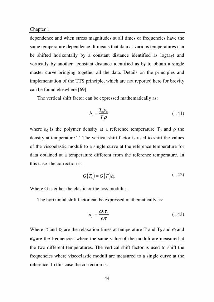
Chapter 1

44

dependence and when stress magnitudes at all times or frequencies have the

same temperature dependence. It means that data at various temperatures can

be shifted horizontally by a constant distance identified as log(aT) and

vertically by another constant distance identified as bT to obtain a single

master curve bringing together all the data. Details on the principles and

implementation of the TTS principle, which are not reported here for brevity

can be found elsewhere [69].

The vertical shift factor can be expressed mathematically as:

b

T=

T0ρ0

T ρ

(1.41)

where is the polymer density at a reference temperature T0 and ρ the

density at temperature T. The vertical shift factor is used to shift the values

of the viscoelastic moduli to a single curve at the reference temperature for

data obtained at a temperature different from the reference temperature. In

this case the correction is:

G T0( ) = G T( )b

T (1.42)

Where G is either the elastic or the loss modulus.

The horizontal shift factor can be expressed mathematically as:

a

T=

ω0τ 0

ωτ

(1.43)

Where τ and τ0 are the relaxation times at temperature T and T0 and ω and

ω0 are the frequencies where the same value of the moduli are measured at

the two different temperatures. The vertical shift factor is used to shift the

frequencies where viscoelastic moduli are measured to a single curve at the

reference. In this case the correction is:

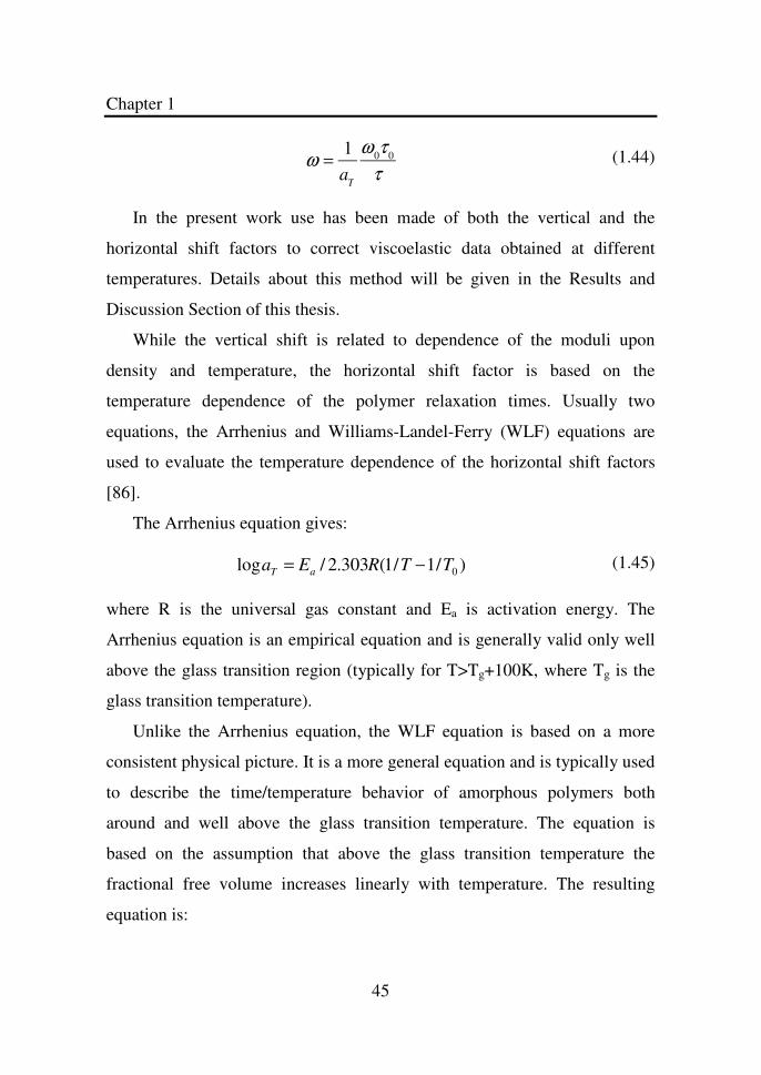
Chapter 1

45

ω =

1a

T

ω0τ 0

τ

(1.44)

In the present work use has been made of both the vertical and the

horizontal shift factors to correct viscoelastic data obtained at different

temperatures. Details about this method will be given in the Results and

Discussion Section of this thesis.

While the vertical shift is related to dependence of the moduli upon

density and temperature, the horizontal shift factor is based on the

temperature dependence of the polymer relaxation times. Usually two

equations, the Arrhenius and Williams-Landel-Ferry (WLF) equations are

used to evaluate the temperature dependence of the horizontal shift factors

[86].

The Arrhenius equation gives:

)/1/1(303.2/log 0TTREa aT −= (1.45)

where R is the universal gas constant and Ea is activation energy. The

Arrhenius equation is an empirical equation and is generally valid only well

above the glass transition region (typically for T>Tg+100K, where Tg is the

glass transition temperature).

Unlike the Arrhenius equation, the WLF equation is based on a more

consistent physical picture. It is a more general equation and is typically used

to describe the time/temperature behavior of amorphous polymers both

around and well above the glass transition temperature. The equation is

based on the assumption that above the glass transition temperature the

fractional free volume increases linearly with temperature. The resulting

equation is:

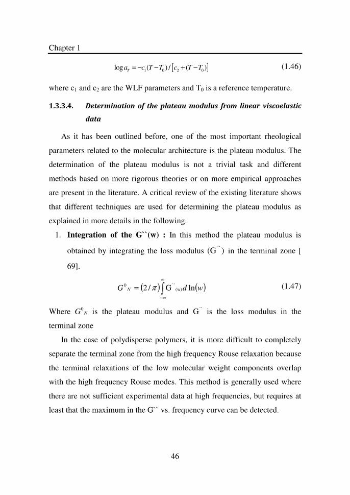
Chapter 1

46

[ ]1 0 2 0log ( ) / ( )T

a c T T c T T= − − + − (1.46)

where c1 and c2 are the WLF parameters and T0 is a reference temperature.

1.3.3.4. Determination of the plateau modulus from linear viscoelastic

data

As it has been outlined before, one of the most important rheological

parameters related to the molecular architecture is the plateau modulus. The

determination of the plateau modulus is not a trivial task and different

methods based on more rigorous theories or on more empirical approaches

are present in the literature. A critical review of the existing literature shows

that different techniques are used for determining the plateau modulus as

explained in more details in the following.

1. Integration of the G``(w) : In this method the plateau modulus is

obtained by integrating the loss modulus )(G `` in the terminal zone [

69].

( ) ( )wdG N lnG/2 (w)``0

∫∞

∞−

= π

(1.47)

Where NG0 is the plateau modulus and ``G is the loss modulus in the

terminal zone

In the case of polydisperse polymers, it is more difficult to completely

separate the terminal zone from the high frequency Rouse relaxation because

the terminal relaxations of the low molecular weight components overlap

with the high frequency Rouse modes. This method is generally used where

there are not sufficient experimental data at high frequencies, but requires at

least that the maximum in the G`` vs. frequency curve can be detected.

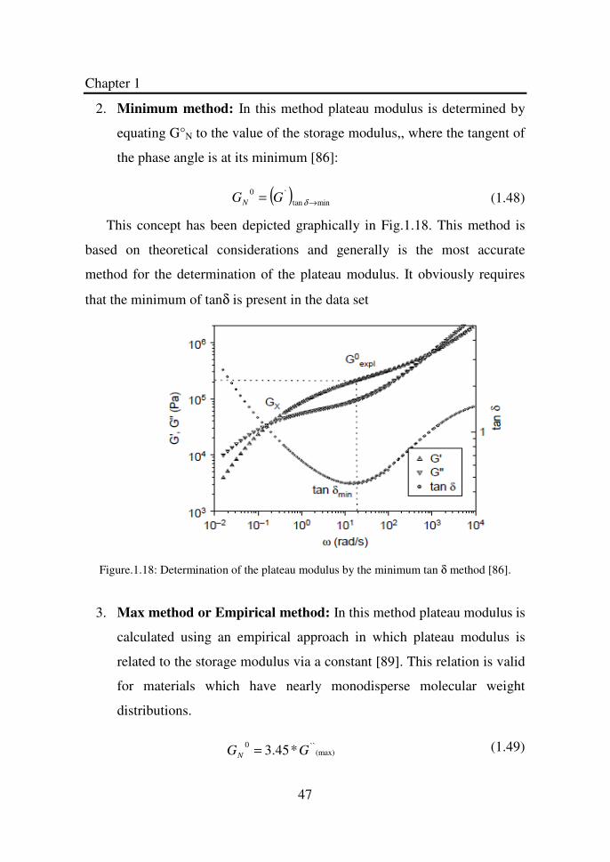
Chapter 1

47

2. Minimum method: In this method plateau modulus is determined by

equating G°N to the value of the storage modulus,, where the tangent of

the phase angle is at its minimum [86]:

( ) mintan`0

→= δGGN

(1.48)

This concept has been depicted graphically in Fig.1.18. This method is

based on theoretical considerations and generally is the most accurate

method for the determination of the plateau modulus. It obviously requires

that the minimum of tanδ is present in the data set

Figure.1.18: Determination of the plateau modulus by the minimum tan δ method [86].

3. Max method or Empirical method: In this method plateau modulus is

calculated using an empirical approach in which plateau modulus is

related to the storage modulus via a constant [89]. This relation is valid

for materials which have nearly monodisperse molecular weight

distributions.

(max)``0 *45.3 GGN = (1.49)

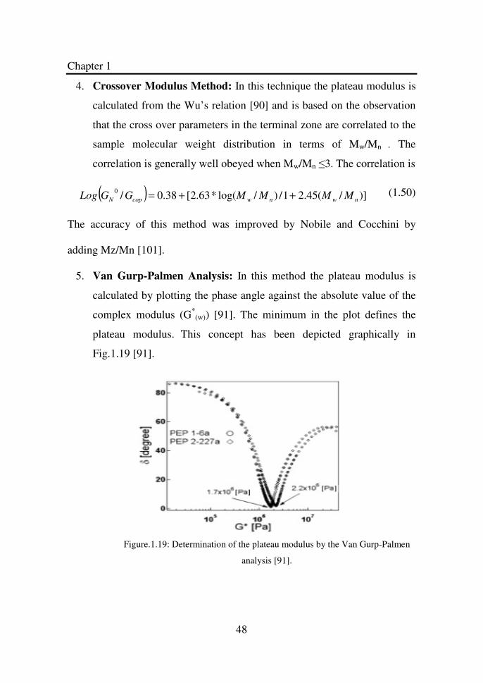
Chapter 1

48

4. Crossover Modulus Method: In this technique the plateau modulus is

calculated from the Wu’s relation [90] and is based on the observation

that the cross over parameters in the terminal zone are correlated to the

sample molecular weight distribution in terms of Mw/Mn . The

correlation is generally well obeyed when Mw/Mn ≤3. The correlation is

( ) )]/(45.21/)/log(*63.2[38.0/0nwnwcopN MMMMGGLog ++= (1.50)

The accuracy of this method was improved by Nobile and Cocchini by

adding Mz/Mn [101].

5. Van Gurp-Palmen Analysis: In this method the plateau modulus is

calculated by plotting the phase angle against the absolute value of the

complex modulus (G*(w)) [91]. The minimum in the plot defines the

plateau modulus. This concept has been depicted graphically in

Fig.1.19 [91].

Figure.1.19: Determination of the plateau modulus by the Van Gurp-Palmen

analysis [91].

Chapter 1

49

1.3.4. Crystallization

When crystalline elastomers are cooled below the thermodynamic

melting temperature, they undergo crystallization. In this section

crystallization and different techniques used for the analysis of polymer

crystallization are discussed and compared. Crystallization is a phase

transition process driven by the excess of thermodynamic free energy in the

system. This generates transport of molecules from the disordered liquid

phase (liquid or melt phase) to the ordered solid phase. In the case of

polymers crystallization is a process associated with the partial alignment of

the molecular chains. Typically, chains fold together and form ordered

regions called lamellae, which compose larger spheroidal structures named

spherulites. Polymers can be crystallized by cooling from the melt, by

mechanical stretching or by solvent evaporation. The first step in polymer

crystallization is the formation of nuclei, which are small units of crystalline

material. The formation of this primary nuclei is called primary

crystallization. It is followed by the induction of more and more polymer on

the growing surface, which is called secondary crystallization or growth.

During the early stages of crystallization, the mechanical response of the

material changes form liquid like to solid like. Crystallinity makes a material

useful. It makes a material strong but it has also demerits. Advantages and

disadvantages of the crystalline material have been discussed in the first

section of this chapter. Different methods (e.g., X-ray scattering, DSC) have

been reported in literature for measuring the crystallinity of polymers.

Rheological methods can also be used as a measure of the crystallization

process. One big advantage of the rheological method is its sensitivity at low

crystallization kinetics, where the more standard DSC technique can fail.

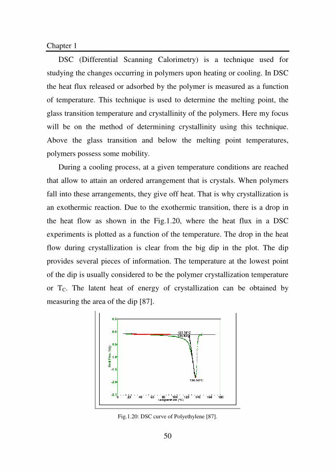
Chapter 1

DSC (Differential Scanning C

studying the changes occurring in polymers

the heat flux released or adsorbed by the polymer is measured as a function

of temperature. This technique is used to determine the melting point,

glass transition temperature and crystallinity of the polymers. Here my focus

will be on the method of determining crystallinity using this technique.

Above the glass transition and below the melting point temperatures,

polymers possess some mobility.

During a cooling process, at a given

that allow to attain an ordered arrangement

fall into these arrangements, they give off heat. That is why crystallization is

an exothermic reaction. Due to the exothermic transition, there is a drop in

the heat flow as shown in the Fig.

experiments is plotted as a function of the temperature

flow during crystallization is clear from the big dip in the

provides several pieces of information. The temperature at the lowest point

of the dip is usually considered to be the polymer

or TC. The latent heat of energy of crystallization

measuring the area of the dip [87].

Fig.1.20: DSC curve of Polyethylene [87].

50

Calorimetry) is a technique used for

in polymers upon heating or cooling. In DSC

the heat flux released or adsorbed by the polymer is measured as a function

This technique is used to determine the melting point, the

glass transition temperature and crystallinity of the polymers. Here my focus

will be on the method of determining crystallinity using this technique.

Above the glass transition and below the melting point temperatures,

given temperature conditions are reached

o attain an ordered arrangement that is crystals. When polymers

fall into these arrangements, they give off heat. That is why crystallization is

to the exothermic transition, there is a drop in

the heat flow as shown in the Fig.1.20, where the heat flux in a DSC

experiments is plotted as a function of the temperature. The drop in the heat

flow during crystallization is clear from the big dip in the plot. The dip

of information. The temperature at the lowest point

y considered to be the polymer crystallization temperature

latent heat of energy of crystallization can be obtained by

Fig.1.20: DSC curve of Polyethylene [87].

Chapter 1

51

The crystallization kinetics, that is the rate at which crystallization occurs

is often studied on the basis of the Avrami model [98,108]. In this model the

isothermal crystallization kinetics is described by the following equation:

])/).(2ln(exp[1)( 5.0n

tttX −−= (1.51)

where X(t) is the relative degree of crystallization (the fraction of polymer

crystallized at time t with respect to the total time), t0.5 is the half

crystallization time and n is the Avrami exponent. The Avrami exponent (n)

can be related to the mechanism of nucleation and form of crystal growth. It

can be obtained from the slope of the linear regression when log[-ln(1-x(t))]

is plotted against log(t). As said before, t0.5 is the time needed to reach a

relative crystallinity of 50%. t0.5 has been also reported in the literature as an

increasing function of crystallization temperature.

)/exp()(5.0 cac RTEATt −= (1.52)

where A is a dimensionless parameter and Ea is the activation energy. Tc is

crystallization temperature. R is the universal gas constant.

In some cases, rheological methods can provide a more sensitive and

accurate measure of the crystallization kinetics. This happens when the

crystallization rates are very low, as it is the case when the crystallization

temperature is close to the thermodynamic limit. In these cases, the heat flux

(which is a measure of the amount of heat released per unit time) can fall

below the sensitivity limits of the calorimetric apparatus. On the contrary,

the rheological measurement monitors the time evolution of the viscoelastic

moduli. These a cumulative measurement and the sensitivity issue do not

apply.

When the polymer is cooled below its melting point, crystallinity starts to

develop and the material transforms into a semi crystalline material and the

viscoelastic properties of the system such as elastic modulus and viscous

Chapter 1

52

modulus change. Rheological parameters can be used to evaluate the relative

crystallinity. Khanna et al. [88], for example suggested a linear relationship

between elastic modulus and crystallinity and used this technique to study

the crystallization kinetics of different polymers [88].

' ' ' '0 0( ) /x t G G G G∞= − − (1.53)

where x(t) = crystallinity,G0` = Initial plateau value of elastic modulus, 'G ∞ =

Final plateau value of elastic modulus and 'G = Elastic modulus at time t.

Numerous research works have been reported in literature on the

crystallization behavior of crystalline elastomers [147-149]. In the present

report an attempt has been made to collect specifically the literature about

the effect of molecular structure on the crystallization process.

Effect of molecular structure such as tacticity and molecular weight on

the crystallization and melting behavior of polypropylene was examined by

Ritva et al., [147]. They prepared polypropylenes of different degree of

syndiotcticity and molecular weights by different heterogenous catalyst

systems. Crystallization and melting experiments were performed using

DSC. For tacticity measurements FT-IR spectroscopy was applied.

Crystallization and thermal properties were found dependent on the tacticity

of the polypropylenes. A linear relationship between tacticity and thermal

properties was noted. No effect of molecular weight in the range of 22000-

97000 was found on the thermal properties of polypropylenes.

In another work crystallization of the syndiotactic polypropylene was

examined as a function of syndiotacticity [148]. In this work the formation of

the trans-planar mesomorphic form at 00C is followed as a function of the

permanence times at 00C by using X-Ray diffraction and FT-IR

spectroscopy. The mesomorphic form of syndiotactic polypropylene(sPP)

was obtained by quenching the melt at 00C and keeping the samples at 00C

Chapter 1

53

for a long time. Samples kept at 00C for a short time rapidly crystallize into

helical form 1 at room temperature, whereas longer permeance time at 00C

increases the stability of the trans-planar mesomorphic form, which remains

stable and inhibits the normal crystallization of the sample into the helical

form at room temperature. It was found that higher the degree of

stereoregularity of the sample, the shorter the permeance time at 00C needed

to stabilize the trans-planar mesomorphic form.

More recently, an investigation on the crystallization from the melt and

of the polymorphic behavior of isotactic poly (1-butene) (iPB) prepared with

metallocene catalysts was carried out. Samples of isotactic polybutene of

different of stereoregularity, containing different concentrations of

stereodefects (rr triads defects) and regiodefects have been prepared with

different C2- and C1-symmetric metallocene catalysts. The concentration of

defects and the molecular mass are controlled by the choice of the catalyst

structure and conditions of polymerization. Highly isotactic samples with

concentration of rr stereodefects lower than 2 mol %, crystallize from the

melt in the metastable form II. This is a common polymorphic behavior

observed in iPB samples prepared with Ziegler-Natta catalysts and

extensively reported in the literature. More stereodefective iPB samples,

containing concentration of stereodefects higher than 2 mol % crystallize

form the melt as mixtures of form II and form I, the fraction of crystals of

form I increases with increasing concentration of defects and decreasing

cooling rate from the melt and samples with concentration of rr defects of 3-

4 mol% crystallize from the melt in the pure form I at low cooling rates. The

results presented in this paper give the first experimental observation of the

crystallization of the stable trigonal form I of iPB from the melt at

atmospheric pressure [149].

Chapter 1

54

In conclusion, it can be said that the crystallization process of polyolefin

based crystalline polymers are affected by the stereo- and region-regularity

of the polymer chain. In nut shell all these phenomena are found to have a

profound influence on the crystallization process and consequently on the

mechanical properties of the solid materials.

1.3.5. Flow induced crystallization

The enhancement in the rate of polymer crystallization due to the

application of shear or extensional flow is known as flow induced

crystallization. In the other word flow induced crystallization can be defined

as the process in which the rate of polymer crystallization is accelerated by

the action of flow. This phenomenon alters both processing and material

final properties. The physics behind flow induced crystallization is simple.

When a polymer is subjected to an extensional or shear flow, the polymer

chains are oriented and stretched. This results in a decrease of the entropy or

equivalent increase in free energy. This increase in free energy acts as a

driving force and thus accelerates the polymer crystallization process by

accelerating the rate of nucleation.

As it was said before, the process of crystallization occurs in two steps.

In the first step formation of nuclei (stable nuclei) occurs, while in the

second step the subsequent growth of crystallites occurs. The flow has an

effect on the first step of crystallization (nucleation stage) [114].

Furthermore, while quiescent crystallization leads to the formation of

spherical, non-oriented structures (spherulites) flow can also determine

oriented crystalline structures, such as fibers. The mechanism of flow

induced crystallization is well documented in the literature [115].

The process can be explained as stretching of long chains to form fibrous

crystals. During the stretching process, the distortion of chains from their

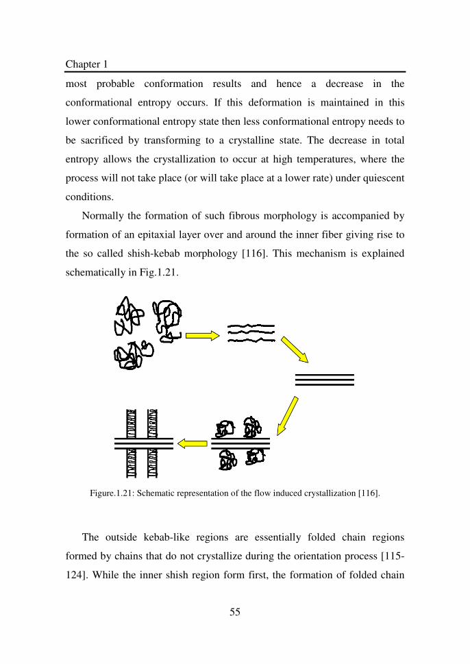
Chapter 1

55

most probable conformation results and hence a decrease in the

conformational entropy occurs. If this deformation is maintained in this

lower conformational entropy state then less conformational entropy needs to

be sacrificed by transforming to a crystalline state. The decrease in total

entropy allows the crystallization to occur at high temperatures, where the

process will not take place (or will take place at a lower rate) under quiescent

conditions.

Normally the formation of such fibrous morphology is accompanied by

formation of an epitaxial layer over and around the inner fiber giving rise to

the so called shish-kebab morphology [116]. This mechanism is explained

schematically in Fig.1.21.

Figure.1.21: Schematic representation of the flow induced crystallization [116].

The outside kebab-like regions are essentially folded chain regions

formed by chains that do not crystallize during the orientation process [115-

124]. While the inner shish region form first, the formation of folded chain

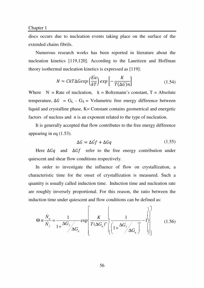
Chapter 1

56

discs occurs due to nucleation events taking place on the surface of the

extended chains fibrils.

Numerous research works has been reported in literature about the

nucleation kinetics [119,120]. According to the Lauritzen and Hoffman

theory isothermal nucleation kinetics is expressed as [119]:

= ∆ −

∆

(1.54)

Where N. = Rate of nucleation, k = Boltzmann’s constant, T = Absolute

temperature, ∆ = GL - GS = Volumetric free energy difference between

liquid and crystalline phase, K= Constant contains geometrical and energetic

factors of nucleus and n is an exponent related to the type of nucleation.

It is generally accepted that flow contributes to the free energy difference

appearing in eq (1.53).

∆ = ∆! + ∆# (1.55)

Here ∆# and ∆! refer to the free energy contribution under

quiescent and shear flow conditions respectively.

In order to investigate the influence of flow on crystallization, a

characteristic time for the onset of crystallization is measured. Such a

quantity is usually called induction time. Induction time and nucleation rate

are roughly inversely proportional. For this reason, the ratio between the

induction time under quiescent and flow conditions can be defined as:

1 1exp 1

( )1 1

q

nnff q f

qq

N K

GN T G GG G

Θ ≡ = − ∆ ∆ ∆ + +∆ ∆

&

&

(1.56)

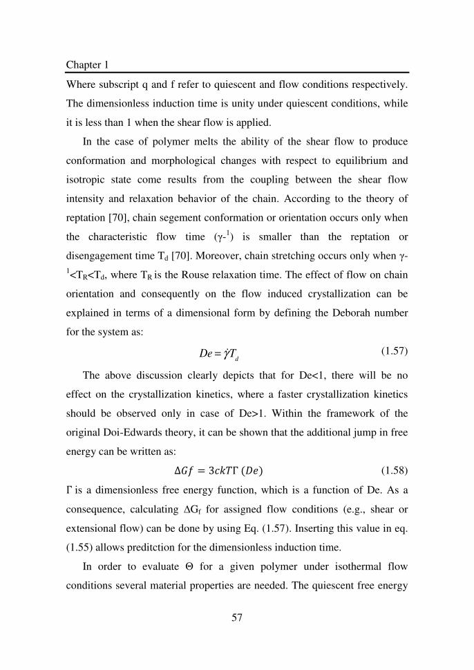
Chapter 1

57

Where subscript q and f refer to quiescent and flow conditions respectively.

The dimensionless induction time is unity under quiescent conditions, while

it is less than 1 when the shear flow is applied.

In the case of polymer melts the ability of the shear flow to produce

conformation and morphological changes with respect to equilibrium and

isotropic state come results from the coupling between the shear flow

intensity and relaxation behavior of the chain. According to the theory of

reptation [70], chain segement conformation or orientation occurs only when

the characteristic flow time (γ-1) is smaller than the reptation or

disengagement time Td [70]. Moreover, chain stretching occurs only when γ-1<TR<Td, where TR is the Rouse relaxation time. The effect of flow on chain

orientation and consequently on the flow induced crystallization can be

explained in terms of a dimensional form by defining the Deborah number

for the system as:

De = &γ T

d (1.57)

The above discussion clearly depicts that for De<1, there will be no

effect on the crystallization kinetics, where a faster crystallization kinetics

should be observed only in case of De>1. Within the framework of the

original Doi-Edwards theory, it can be shown that the additional jump in free

energy can be written as:

∆! = 3%Γ( (1.58)

Γ is a dimensionless free energy function, which is a function of De. As a

consequence, calculating ∆Gf for assigned flow conditions (e.g., shear or

extensional flow) can be done by using Eq. (1.57). Inserting this value in eq.

(1.55) allows preditction for the dimensionless induction time.

In order to evaluate Θ for a given polymer under isothermal flow

conditions several material properties are needed. The quiescent free energy

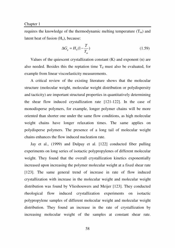
Chapter 1

58

requires the knowledge of the thermodynamic melting temperature (Tm) and

latent heat of fusion (Ho), because:

0 (1 )q

m

TG H

T∆ = − (1.59)

Values of the quiescent crystallization constant (K) and exponent (n) are

also needed. Besides this the reptation time Td must also be evaluated, for

example from linear viscoelasticity measurements.

A critical review of the existing literature shows that the molecular

structure (molecular weight, molecular weight distribution or polydispersity

and tacticity) are important structural properties in quantitatively determining

the shear flow induced crystallization rate [121-122]. In the case of

monodisperse polymers, for example, longer polymer chains will be more

oriented than shorter one under the same flow conditions, as high molecular

weight chains have longer relaxation times. The same applies on

polydisperse polymers. The presence of a long tail of molecular weight

chains enhances the flow induced nucleation rate.

Jay et al., (1999) and Dulpay et al. [122] conducted fiber pulling

experiments on long series of isotactic polypropylenes of different molecular

weight. They found that the overall crystallization kinetics exponentially

increased upon increasing the polymer molecular weight at a fixed shear rate

[123]. The same general trend of increase in rate of flow induced

crystallization with increase in the molecular weight and molecular weight

distribution was found by Vlieshouwers and Meijer [123]. They conducted

rheological flow induced crystallization experiments on isotactic

polypropylene samples of different molecular weight and molecular weight

distribution. They found an increase in the rate of crystallization by

increasing molecular weight of the samples at constant shear rate.

Chapter 1

59

Furthermore they found that after a combined thermo mechanical treatment

that mainly caused a degradation of the high molecular weight tail, the effect

of the shear rate on the crystallization rate was strongly reduced.

Monasse and his coworkers have examined the influence of molecular

structure of polypropylene on the crystallization, both quiescent and shear

induced [121,122]. They showed that in quiescent conditions the higher

degree of isotacticity and the decrease in chain defects weakly enhanced the

growth rate of crystalline structures, whereas the molecular weight (Mw) and

molecular weight distribution (MWD) were found to be less relevant

parameters. The independence of the kinetics on Mw was explained taking

into account that during the growth mechanism only a small portion of chain

(order of 100 monomers) is involved in the deposit of crystalline segment at

the growth front. This amount is negligible in comparison to the high degree

of polymerization [128]. On the contrary, during shear the growth rate was

governed by molecular weight. A critical molecular weight value, related to

the critical mass between entanglements, below which the polymer is

insensitive to shear flow, was obtained by Haudin et al. [130].

The influence of the molecular weight on flow induced crystallization

has been also investigated by Bove and Nobile [131,132]. They used

rheological measurements to investigate the evolution of crystallization in

quiescent conditions as well as after the application of a shear flow. Strong

enhancement in crystallization kinetics was observed when the step shear

flow was applied on poly(1-butene) samples (PB) with different Mw and on

a polypropylene sample (PP). They also found that a critical shear rate (at a

constant strain) coupled to a critical shear strain (at a constant shear rate) are

necessary to obtain the enhancement of the overall-crystallization rate.

Chapter 1

60

Moreover, a relevant molecular weight effect was noted in the step shear

flow crystallization, while in quiescent conditions no evidence was found.

Recently, Acierno et al. [133] have explained the combined effects of

shear flow and polymer molecular weight introducing the dimensionless

Weissenberg number, Wi, i.e. the product of the relaxation time inherent to

the material and the deformation rate for the flow process. They analyzed the

influence of shear flow on the crystallization of a sequence of Polybutenes

with different Mw, and found that the application of a shear flow

significantly accelerates the crystallization kinetics, as reflected by a faster

light intensity dynamics in turbidity measurements. By the definition of a

dimensionless crystallization time, obtained normalizing the crystallization

time after shear with the same time in static conditions, it was shown that the

kinetic deviation from quiescent state occurs at lower shear rates as the

molecular weight increases. They also showed that the dimensionless

crystallization times of different molecular weight PB falls on the same

master curve if they are plotted against the Weissenberg number (Wi).

More recently, Fenguan et al. [125] obtained the same results by

investigating the process using differential scanning calorimetry (DSC),

rheological techniques, polarized optical microscope and X-ray diffraction

techniques. They performed experiments on both linear and branched chain

polypropylene. Long chain branched polypropylene showed accelerated

crystallization kinetics in comparison with that of low branched chains. The

crystallization of long chain branched polypropylene was found more

sensitive to shear flow than that of linear polypropylene during the induced

period at low shear rates, which indicates that the longer relaxation time of

the polymer chains plays an important role in the nucleation of

polypropylene under shear flow fields.

Chapter 1

61

As mentioned earlier the application of flow to increase the rate of

crystallization can be shear or extensional. Extensional flow means a type of

deformation which involves the elongation or stretching of a viscous material

[127]. Extensional flow is expected to produce more relevant effects than

shear in flow-induced crystallization [134]. Extensional flow is more

sensitive to the molecular structure of the polymer than the shear flow. For

example, at the same level of, it generates a much higher degree of molecular

orientation and stretching than the simple shear. The strain requirement for

the flow induced crystallization is less in extension than in the shear.

Another difference of extensional flow with respect to simple shear is the

absence of slip issue. Slip is a relevant problem in simple shear because it

reduces the applied shear deformation, making it very difficult to remove the

effects of slip from the physical response of the material to deformation

[135].

Both extensional and shear flows produce alignment, which enhance the

crystallization process. Literature data suggest that flow induced

crystallization can reduce the induction time of crystallization by several

orders of magnitude, when compared to quiescent crystallization [135, 136].

As in the case of shear flow, the effect of extensional flow depends upon on

the strength of flow, which can be characterized by the Weissenberg number.

Hadinata et al. [141] studied and compared both the extensional flow and

shear flow induced crystallization of a high molecular weight isotactic poly-

1-butene. They used an extensional viscosity fixture on a rotational

rheometer to apply an extensional flow to the melts. They found that the flow

induced crystallization occurring in the extensional flow is much stronger

than that observed under shear. They also found that beyond a critical

Chapter 1

62

extension rate, the onset of crystallization time decreased roughly with the

inverse of the extension rate.

Sentmanat et al. [142] used the Sentmanat extensional viscosity fixture

on a rotational rheometer, which is similar to extensional viscosity fixture

used by Hadinata et al. [138]. They handled the problem of sample sagging

in the rheometer by quenching the samples with water after the application of

extensional flow. Their findings indicate that a higher degree of

crystallization can be achieved by the application of extensional flow near

the melting temperature.

More recently, Chellamuthu et al. [143] conducted extensional flow

induced crystallization measurements of isotactic poly-1-butene using a

filament stretching rheometer. They found that extensional flow is effective

in enhancing the polymer crystallization process. They conducted DSC and

small angle X-ray scattering measurements for the estimation of the degree

of crystallinity and found an increase in the degree of crystallinity from 45 to

62% with an increase in the extension rate from 0.01s-1 to 50s-1 for a fixed

imposed strain. Moreover, they found that below a threshold extension rate

no flow induced crystallization occurs. Conversely, a decrease in flow

induced crystallization above a second critical threshold was also found.

Chapter 2

63

Experimental Methods

In the present work linear viscoelasticity, quiescent crystallization and

extensional flow induced crystallization of polypropylene and poly-1Butene

were investigated. To this end, different experimental apparatuses were used.

Linear viscoelasticity in shear oscillatory flow was performed by means of

an Advanced Rheometric Expansion System (ARES, TA Instruments Ltd)

strain controlled rotational rheometer. The ARES rheometer was also used

for extensional measurements. In this case it was equipped by the using the

Sentamanat Extensional Rheometer (SER, Xpansion Company) fixture.

Differential Scanning Calorimetry was performed by means of a Shimadzu

60 calorimeter (Shimadzu Corporation).

2.1. Linear Viscoelasticity

Numerous experimental techniques have been reported in the literature

for the measurement of viscoelasticity of elastomers. But the recommended

one and the most used experimental technique is the dynamic oscillatory

method. A general advantage of this method is that a single instrument can

cover a wide range of frequency. Viscoelastic measurements of elastomers

can be carried out by dynamic method successfully either by applying a

constant strain or stress.

Oscillatory shear is the most popular and common because it is easier to

measure the storage and loss moduli using the oscillatory shear experiments

than to generate the step strains or stresses and measure the resulting stress

or strain. In oscillatory shear experiments, the sample is subjected to a

Chapter 2

64

homogenous deformation at a sinusoidally varying strain or shear stress. In a

controlled strain experiment, one generates a strain that is as close as

possible to a sine wave [13].

γ = γ0sin(ωt) (2.1)

If the strain amplitude is sufficiently small, so that the response is linear,

the resulting stress is also sinusoidal and can be written in terms of the stress

amplitude ( 0σ ) and the phase angle also called loss angle (δ ).

σ (t) = σ0sin(ωt +δ ) (2.2)

Viscoelastic experiments are performed in the frequency domain rather

than in the time domain. Since in an oscillatory experiment with a sine wave

input, the resulting stress wave form is fitted to a sinusoidal function at each

frequency and this fitting process acts as a filter that rejects noise which is

non-sinusodial or is at a frequency other than imposed. This noise rejection

technique improves with increasing number of measuring cycles.

In the case of a linear system in the frequency domain, the results can be

expressed in terms of the amplitude ratio Gd = σ0/γ0 and a phase angle (δ)

which are functions of frequency. The dynamic test results are usually

reported in terms of the storage and loss moduli (G` and G``) as a function of

frequency.

σ (t) = γ 0[ ′G (ω )sin(ωt) + ′′G (ω )cos(ωt)] (2.3)

It is sometimes useful to express the dynamic data in terms of the loss

and storage moduli by considering it the imaginary and real parts of the

complex modulus (G*).

G* = ′G (ω ) + i ′′G (ω ) (2.4)

It follows that the magnitude of the complex modulus is given by:

Chapter 2

65

G

* = ′G( )2

+ ′′G( )2

(2.5)

The dynamic data can be expressed alternatively in terms of a complex

viscosity ( *η ):

η* =

G*

iω=

1ω

′′G − i ′G (ω )( ) = ′η − i ′′η

(2.6)

η* =

G*

ω=

′G( )2

+ ′′G( )2

ω

(2.7)

The complex viscosity is a particular useful quantity when the viscous

behavior of viscoelastic polymer melts is to be studied. In the limit of zero

shear rate, continuum mechanics imposes that [69]:

′η ω( )ω→0

=′′G ω( )ω

ω→0

= η &γ( )&γ →0

(2.8)

In the case of viscoelastic fluids, the elastic component to η` disappears

in the low frequency limit, and one has:

η* ω( )

ω→0= η &γ( )

&γ →0= η0

(2.9)

Where η0 is the zero-shear rate viscosity. For most linear polymer melts, as it

is the case for the crystalline elastomers investigates in the present work, the

empirical Cox-Merz rule often applies [69]:

η* ω( ) ≅ η &γ( ) (2.10)

Even in the case of non-vanishing frequencies and shear rate. The

consequence of Eq. (2.10) is that the steady-shear viscosity curve as a

function of shear rate can be obtained by performing a linear viscoelastic

frequency response measurement of the polymer melt. All quantities

described above have been measured in the present work by using an ARES

strain controlled rotational rheometer (TA Instruments). Data acquisition and

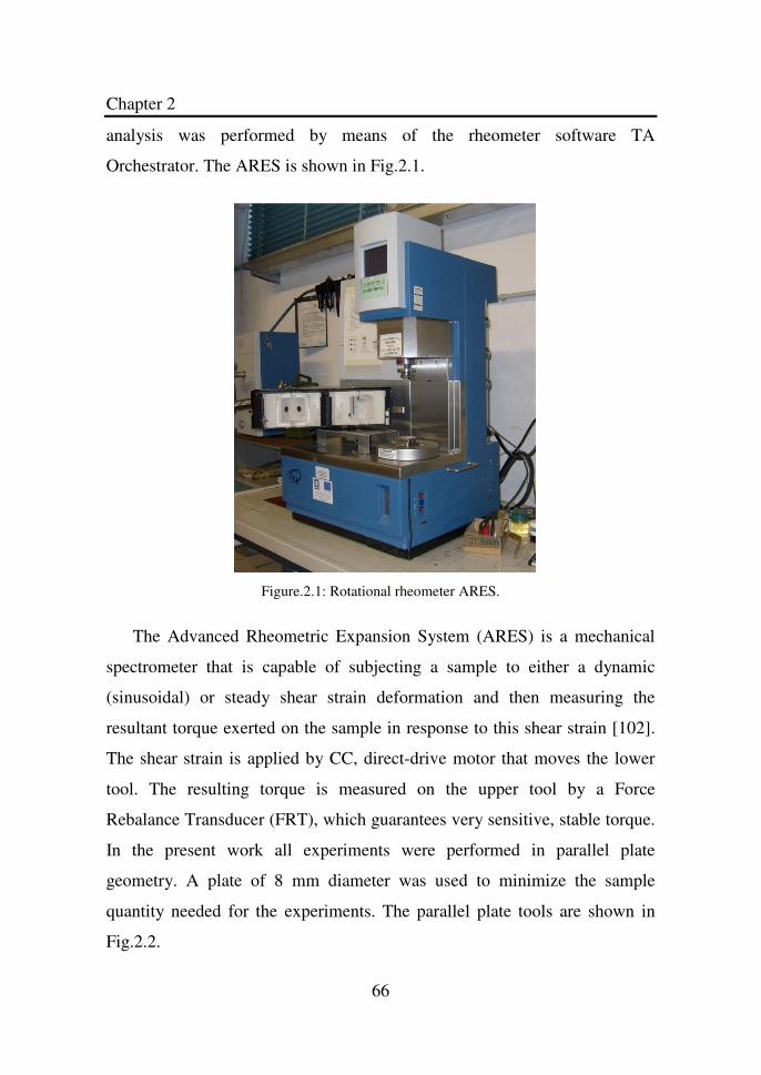
Chapter 2

66

analysis was performed by means of the rheometer software TA

Orchestrator. The ARES is shown in Fig.2.1.

Figure.2.1: Rotational rheometer ARES.

The Advanced Rheometric Expansion System (ARES) is a mechanical

spectrometer that is capable of subjecting a sample to either a dynamic

(sinusoidal) or steady shear strain deformation and then measuring the

resultant torque exerted on the sample in response to this shear strain [102].

The shear strain is applied by CC, direct-drive motor that moves the lower

tool. The resulting torque is measured on the upper tool by a Force

Rebalance Transducer (FRT), which guarantees very sensitive, stable torque.

In the present work all experiments were performed in parallel plate

geometry. A plate of 8 mm diameter was used to minimize the sample

quantity needed for the experiments. The parallel plate tools are shown in

Fig.2.2.

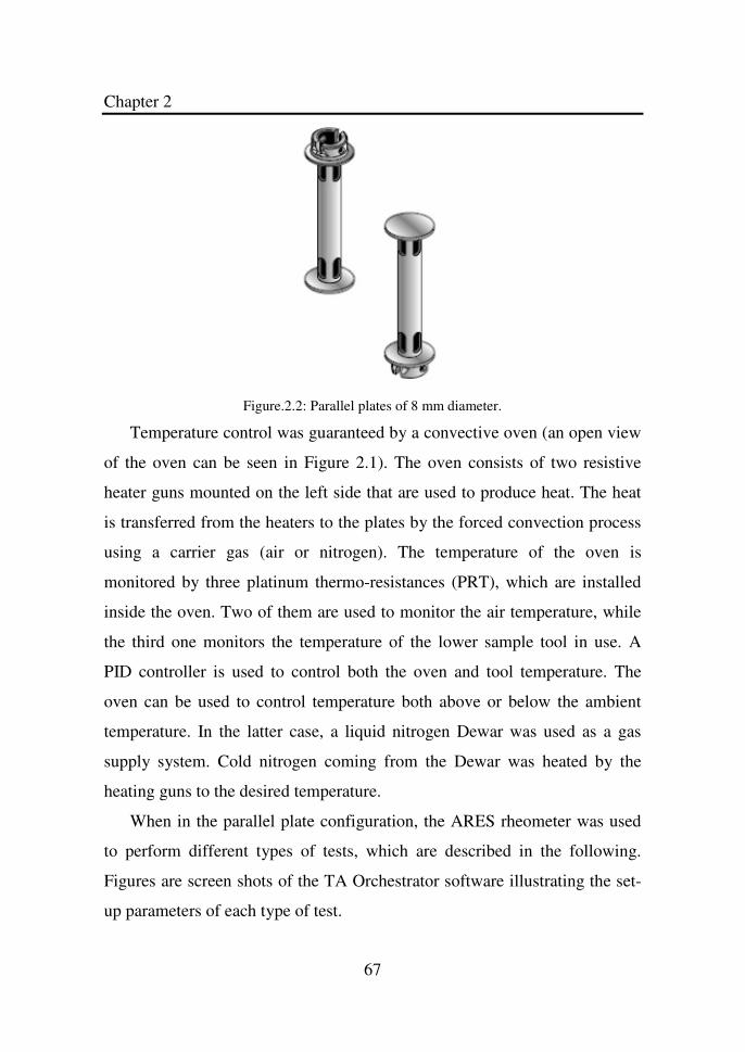
Chapter 2

67

Figure.2.2: Parallel plates of 8 mm diameter.

Temperature control was guaranteed by a convective oven (an open view

of the oven can be seen in Figure 2.1). The oven consists of two resistive

heater guns mounted on the left side that are used to produce heat. The heat

is transferred from the heaters to the plates by the forced convection process

using a carrier gas (air or nitrogen). The temperature of the oven is

monitored by three platinum thermo-resistances (PRT), which are installed

inside the oven. Two of them are used to monitor the air temperature, while

the third one monitors the temperature of the lower sample tool in use. A

PID controller is used to control both the oven and tool temperature. The

oven can be used to control temperature both above or below the ambient

temperature. In the latter case, a liquid nitrogen Dewar was used as a gas

supply system. Cold nitrogen coming from the Dewar was heated by the

heating guns to the desired temperature.

When in the parallel plate configuration, the ARES rheometer was used

to perform different types of tests, which are described in the following.

Figures are screen shots of the TA Orchestrator software illustrating the set-

up parameters of each type of test.

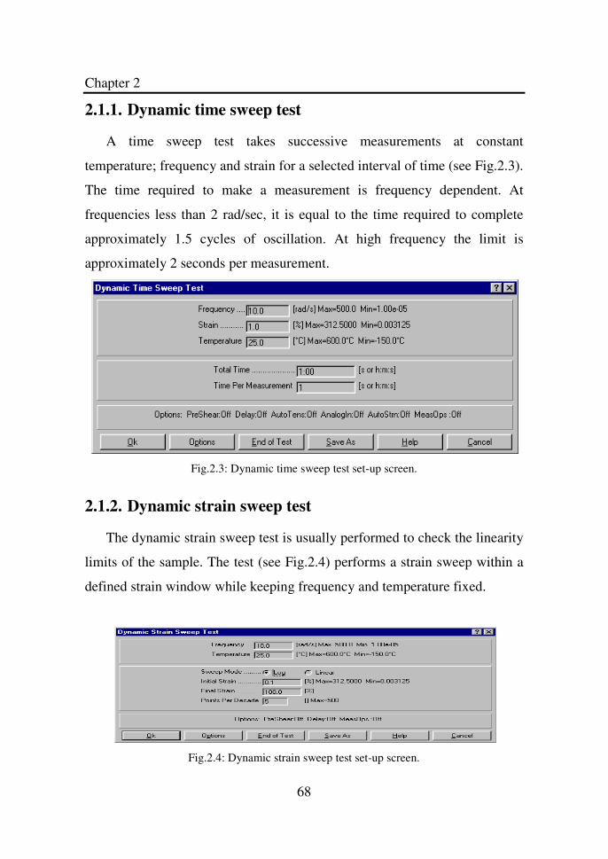
Chapter 2

68

2.1.1. Dynamic time sweep test

A time sweep test takes successive measurements at constant

temperature; frequency and strain for a selected interval of time (see Fig.2.3).

The time required to make a measurement is frequency dependent. At

frequencies less than 2 rad/sec, it is equal to the time required to complete

approximately 1.5 cycles of oscillation. At high frequency the limit is

approximately 2 seconds per measurement.

Fig.2.3: Dynamic time sweep test set-up screen.

2.1.2. Dynamic strain sweep test

The dynamic strain sweep test is usually performed to check the linearity

limits of the sample. The test (see Fig.2.4) performs a strain sweep within a

defined strain window while keeping frequency and temperature fixed.

Fig.2.4: Dynamic strain sweep test set-up screen.

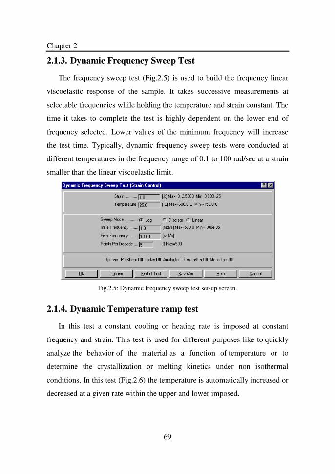
Chapter 2

69

2.1.3. Dynamic Frequency Sweep Test

The frequency sweep test (Fig.2.5) is used to build the frequency linear

viscoelastic response of the sample. It takes successive measurements at

selectable frequencies while holding the temperature and strain constant. The

time it takes to complete the test is highly dependent on the lower end of

frequency selected. Lower values of the minimum frequency will increase

the test time. Typically, dynamic frequency sweep tests were conducted at

different temperatures in the frequency range of 0.1 to 100 rad/sec at a strain

smaller than the linear viscoelastic limit.

Fig.2.5: Dynamic frequency sweep test set-up screen.

2.1.4. Dynamic Temperature ramp test

In this test a constant cooling or heating rate is imposed at constant

frequency and strain. This test is used for different purposes like to quickly

analyze the behavior of the material as a function of temperature or to

determine the crystallization or melting kinetics under non isothermal

conditions. In this test (Fig.2.6) the temperature is automatically increased or

decreased at a given rate within the upper and lower imposed.

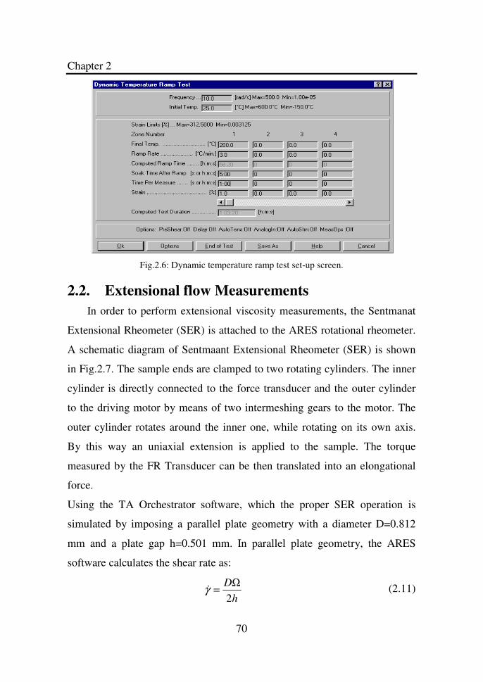
Chapter 2

70

Fig.2.6: Dynamic temperature ramp test set-up screen.

2.2. Extensional flow Measurements

In order to perform extensional viscosity measurements, the Sentmanat

Extensional Rheometer (SER) is attached to the ARES rotational rheometer.

A schematic diagram of Sentmaant Extensional Rheometer (SER) is shown

in Fig.2.7. The sample ends are clamped to two rotating cylinders. The inner

cylinder is directly connected to the force transducer and the outer cylinder

to the driving motor by means of two intermeshing gears to the motor. The

outer cylinder rotates around the inner one, while rotating on its own axis.

By this way an uniaxial extension is applied to the sample. The torque

measured by the FR Transducer can be then translated into an elongational

force.

Using the TA Orchestrator software, which the proper SER operation is

simulated by imposing a parallel plate geometry with a diameter D=0.812

mm and a plate gap h=0.501 mm. In parallel plate geometry, the ARES

software calculates the shear rate as:

h

D

2Ω

=γ&

(2.11)

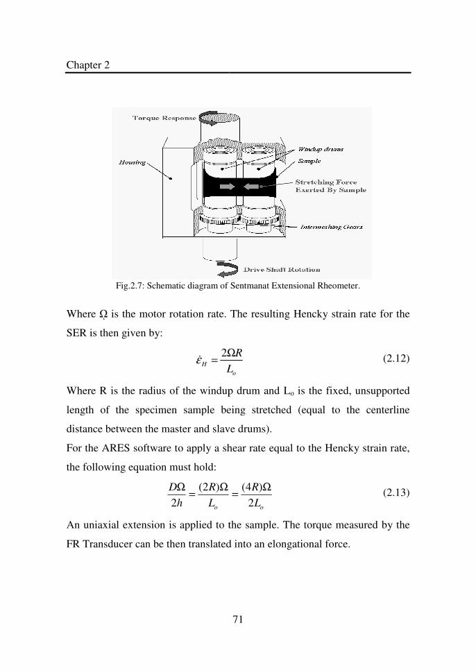
Chapter 2

Fig.2.7: Schematic diagram of Sentmanat Extensional Rheometer.

Where ῼ is the motor rotation rate. The

SER is then given by:

HL

Ω=

2ε&

Where R is the radius of the windup drum and L

length of the specimen sample being stretched (equal to the centerline

distance between the master and slave drums).

For the ARES software to apply a shear rate equal to the Hencky strain rate,

the following equation must hold:

oL

R

h

D )2(2

Ω=

Ω

An uniaxial extension is applied to the sample. The torque measured by the

FR Transducer can be then translated i

71

Fig.2.7: Schematic diagram of Sentmanat Extensional Rheometer.

is the motor rotation rate. The resulting Hencky strain rate for the

oL

RΩ

(2.12)

R is the radius of the windup drum and Lo is the fixed, unsupported

length of the specimen sample being stretched (equal to the centerline

distance between the master and slave drums).

For the ARES software to apply a shear rate equal to the Hencky strain rate,

oL

R

2)4( Ω

=

(2.13)

uniaxial extension is applied to the sample. The torque measured by the

FR Transducer can be then translated into an elongational force.

Chapter 2

72

Thus, specifying D=4R=0.812 mm and h=Lo=0.501 mm will ensure that the

specified extensional rate for the test will be equal to the Hencky strain rate.

This is true as long as the dimensional ratio is constant (D/h =1.62).

2.2.1. Test Setup

To perform extensional flow measurements, the windup drums must

operate at a constant rate of rotation. This can be achieved by operating the

ARES to perform step rate test using the steady motor and transient

measurement type. Under this set-up, the data acquisition rates can be

separated into four zones, which allow faster data sampling at shorter times

(which is essential for high extensional deformation rate) and slower data

sampling at longer times. During the test temperature control is achieved by

controlling temperature of the oven. This is done by selecting the oven air

PRT in the temperature control loop.

2.2.2. Data analysis

The required data obtained from the ARES rheometer is the shear rate

(equal to the Hencky strain rate), time and the corresponding torque. In many

experiments below a Hencky strain rate of 1 s-1, there may be a small initial

time offset visible in the data due to the slight “slack” due to sample loading

and melt expansion. This slight deformation delay is highly exaggerated on a

log-log plot, but is negligible on a linear plot. Therefore, a time offset must

be incorporated for such experiments. The time offset varies from test to test,

depending on the “slack” that exists in the sample, and thus it must be

evaluated in each case. At the same time, it may be necessary to correct the

collected torque data for any residual stress in the sample due to sample

loading. Again, the torque offset varies from test to test, but at high

Chapter 2

73

temperature measurements, it is rare that one needs to incorporate any torque

offset.

Once the torque measurement data are available, the time dependent

tensile force ( )tFE can be calculated from the torque as:

( )R

TTtF

offset

E 2

−=

(2.14)

where T is the torque and again R is the radius of the windup drum.

If there is no deviation between the nominal and actual strain rates, the

instantaneous cross sectional area, ( )tA of the stretched specimen changes

exponentially with time t and for a constant Hencky strain rate it can be

expressed as:

( ) [ ]tAtA Ho ε&−= exp

(2.15)

For polymer melts, the specimen exhibits a decrease in density upon

melting which is manifested as a volumetric expansion of the specimen

while loaded on the SER. To account for this dimensional expansion for the

polymer melt, a density correction can be incorporated as follows:

( ) [ ]tAtA H

M

So ε

ρ

ρ&−

= exp

32

(2.16)

where Sρ is the solid state density and Mρ is the melt density of the polymer

at the experimental temperature. Thus the tensile stress growth function,

( )tE

+η can be found using the following equation:

( ) ( )( )

( )( )( ) ( ) [ ]( )[ ]offsetHMSoH

offset

H

E

ttAR

TT

tA

tFt

−−

−==+

ερρεεη

&&& exp2 32

(2.17)

In extension flow measurements, the tensile stress growth coefficient is

plotted against time.

Chapter 2

74

2.3. Differential Scanning Calorimetry

Differential Scanning Calorimetry, DSC, is a thermo-analytical technique

used quantitatively to describe the phase transitions occurring in a material.

In DSC the difference between the amount of heat required to increase the

temperature of the sample and that required to heat a reference material are

measured as a function of temperature. Both sample and reference are

maintained at nearly the same temperature throughout the experiment.

Generally, the temperature program for a DSC analysis is designed so that

the sample holder temperature increases linearly as a function of time.

Alternatively, isothermal temperature tests can be also performed. Only a

few milligrams of material are required to run the analysis.

2.3.1. Working Principle

When a material undergoes a physical transformation such as a phase

transition (crystallization, glass transition), more or less heat will be needed

to flow to it with respect to the reference sample (typically, an empty sample

pan) to maintain both at the same temperature. Whether more or less heat

must flow to the sample depends on the direction of the process (exothermic

or endothermic). For example, when a solid sample melts to a liquid it will

require more heat flowing to the sample than to the reference to increase its

temperature at the same rate. This is due to the absorption of heat by the

sample as it undergoes the endothermic phase transition from solid to liquid.

Likewise as the sample undergoes an exothermic process (such as

crystallization) less heat is required to raise the sample temperature. By

measuring the difference in heat flow between the sample and reference,

DSC is able to measure the amount of heat absorbed or released during such

transitions. DSC may also be used to observe more subtle phase changes,

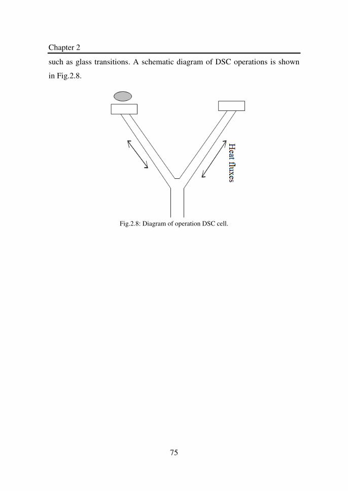
Chapter 2

75

such as glass transitions. A schematic diagram of DSC operations is shown

in Fig.2.8.

Fig.2.8: Diagram of operation DSC cell.

Chapter 3

76

Linear Viscoelasticity of Syndiotactic

Polypropylenes

3.1. Introduction

Mechanical properties like high rigidity, high stress to break and

viscoelastic properties like high deformability and ductility have made

crystalline elastomers an attractive and promising class of innovative

materials for applications in different areas [59,101]. Among crystalline

polyolefins, syndiotactic polypropylene (sPP) has shown interesting and

unexpected elastic properties [59]. In the case of sPP, the crystallization

behavior is strictly related to the degree of tacticity of the polymer, that is to

the local molecular architecture. In turn, a change in tacticity generates

changes in the molecular weight between entanglements, Me, of the polymer

in the melt phase [69, 70]. Since Me is directly related to the viscoelastic

plateau modulus of the melt, it is expected that information on the degree of

tacticity can be extracted from linear viscoelastic measurements in the melt

state. Here, the basis for these relations, which were already presented in the

Introduction chapter, is briefly revisited.

In their fundamental review paper of 1994, Fetters et al. [71] proposed a

simple model to calculate the molecular weight between entanglements and

to relate it to other molecular properties of the polymer chain to some

macroscopic, measurable parameters. The starting point of the model is the

distinction between the volume "occupied" by a chain and the volume

"pervaded" by the same chain. The volume occupied by a chain is the actual

volume filled by the chain. It can be written as:

Chapter 3

77

V =M

ρNA

(3.1)

Where M is the molecular weight, ρ is the density and NA is the Avogadro's

number. The volume spanned by the chain is the portion of space spanned by

the chain. It is chosen by Fetters et al. as:

V

sp= A R

g

2

0

32

(3.2)

In Eq. (3.2) A is a constant of order unity and Rg is the so-called radius of

gyration, such that its mean square value is given by:

R

g

2

0=

R2

0

6=

C∞

M

m0

l02

6

(3.3)

In Eq. (3.3)

R2

0is the mean square end-to-end radius, C∞ is the

characteristic ratio, m0 is the molecular weight and l0 the length of a chain

monomer. Based on Eq. (3.2) the pervaded volume can be written as:

Vsp

= AC

∞M

6m0

32

l03

(3.4)

We now call N the number of polymer chains that fill the pervaded volume.

This will be given by the ratio of the two above defined volumes:

N =V

sp

V= AN

A

C∞

6m0

32

l03M

12

(3.5)

From Eq.(3.5) the molecular weight between entanglements, Me, can be

defined as the chain molecular weight such that N=2. In fact, if M< Me or

N<2, there is not a full second chain in the volume occupied by the test

Chapter 3

78

chain, so there is no entanglement. Based on this definition, Me can be

written as:

Me

=1

B2

R2

0

M

3

ρ 2N

A

2

(3.6)

In Eq. (3.6) the constant B is given by:

B =

A

12 6

(3.7)

It must be noticed that Me is a property of the polymer network. At the

same time, however, it is completely defined by single chain parameters and

by the polymer density. Another molecular quantity of interest is the so-

called packing length [75], defined as:

p =M

ρNA

1

R2

0

=M

eB

ρNA

13

(3.8)

Based on Eq. (3.1) p can be seen as follows. Take a chain spanning the

volume Vsp and squeeze it to its real volume so that it occupies the volume of

a disk-like cylinder whose radius is given (approximately) by

R2

0

12 . Then p

is the thickness of that disk. The packing length can be also seen as a

measure of the lateral size of the polymer chain. By assuming that a chain is

made of a sequence of freely-joined cylinders of diameter d and length bk,

then [148]:

p =

π

4d

2

bK

(3.9)

Larger values of p imply that chain segments are shorter and fatter so that

within the spanned volume, there is less room left for other chains. As a

Chapter 3

79

consequence, larger packing lengths determine a reduced tendency for the

chain to become entangled. The expressions for the Me and p derive from

"geometrical" considerations about the space filling of the polymer melt. The

connection between these quantities and the macroscopic rheological

parameters is given by a suitable theory for chain dynamics. In particular, if

the Doi-Edwards model is used, then the following expression for the plateau

modulus applies:

G

N

0 =45

ρNAkT

Me

(3.10)

As a consequence, measurements of the plateau modulus can directly

yield the value of the molecular weight between entanglements. Conversely,

independent measurements of the ratio between the average chain size and

the polymer molecular weight,

R2

M (for example, by Small Angle Neutron

Scattering) can lead to predictions for the packing length. Furthermore, the

second equality of Eq. (3.8) allows for a quantitative determination of the

parameter A (from B through Eq. (3.7)) and therefore to Me (through Eq.

(3.6)) and to the plateau modulus (through Eq.(3.10)).

Following these lines Fetters et al. [71], analyzed 26 different polymers

for which both SANS measurements of

R2

M and viscoelastic

measurements of GN

0 were available. As already mentioned in Chapter 1,

they found a "universal" correlation between the different parameters. In

particular, at a temperature of 140°C, the fit of the data with a single value of

A=1.518 gave excellent quantitative agreement for all polymers. As a

consequence the following quantitative relationships were established:

Chapter 3

80

GN

0 = 12.16 p−3 (3.11)

Me= 225.8 p

3ρ (3.12)

The numerical factor in Eq. (3.12) has units cm3Å-3mol-1 and that in Eq.

(3.11) MPa Å3.

In the present chapter the viscoelasticity response of a series of

syndiotactic polypropylenes of varying degrees of syndiotacticty has been

investigated. Quantitative values of the plateau modulus have been

determined and, by use of the quantitative relations reported above they have

been translated into molecular information by determining the corresponding

molecular weight between entanglements and packing length. The results

have been compared with existing data on syndiotactic polypropylene and

interpreted in terms of the effect that the degree of stero-regularity has on the

polymer melt organization and on the rheological response.

3.2. Experimental Section

3.2.1. Materials

Samples of sPP with different degrees of syndiotacticity were used for

the viscoelastic study. They were provided by the Department of Chemistry

of the University of Naples. All samples were provided in the form of

thermally compressed films of about 0.5 mm thickness. The relevant

properties of the polymers are reported in Table3.1. Samples labeled sPP-9

and sPP-5 are commercial polymers (supplied by Montell Technology). The

others come from laboratory synthesis using metallocene catalysts [44-50]. It

can be noted from Table.3.1 that samples are characterized by varying

degree of syndiotacticity (%rrrr), melting temperature (Tm) and molecular

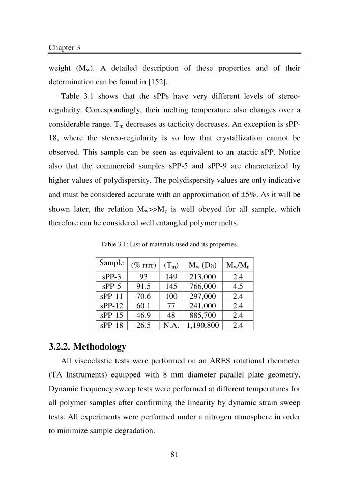
Chapter 3

81

weight (Mw). A detailed description of these properties and of their

determination can be found in [152].

Table 3.1 shows that the sPPs have very different levels of stereo-

regularity. Correspondingly, their melting temperature also changes over a

considerable range. Tm decreases as tacticity decreases. An exception is sPP-

18, where the stereo-regiularity is so low that crystallization cannot be

observed. This sample can be seen as equivalent to an atactic sPP. Notice

also that the commercial samples sPP-5 and sPP-9 are characterized by

higher values of polydispersity. The polydispersity values are only indicative

and must be considered accurate with an approximation of ±5%. As it will be

shown later, the relation Mw>>Me is well obeyed for all sample, which

therefore can be considered well entangled polymer melts.

Table.3.1: List of materials used and its properties.

Sample (% rrrr) (Tm) Mw (Da) Mw/Mn

sPP-3 93 149 213,000 2.4 sPP-5 91.5 145 766,000 4.5

sPP-11 70.6 100 297,000 2.4 sPP-12 60.1 77 241,000 2.4 sPP-15 46.9 48 885,700 2.4 sPP-18 26.5 N.A. 1,190,800 2.4

3.2.2. Methodology

All viscoelastic tests were performed on an ARES rotational rheometer

(TA Instruments) equipped with 8 mm diameter parallel plate geometry.

Dynamic frequency sweep tests were performed at different temperatures for

all polymer samples after confirming the linearity by dynamic strain sweep

tests. All experiments were performed under a nitrogen atmosphere in order

to minimize sample degradation.

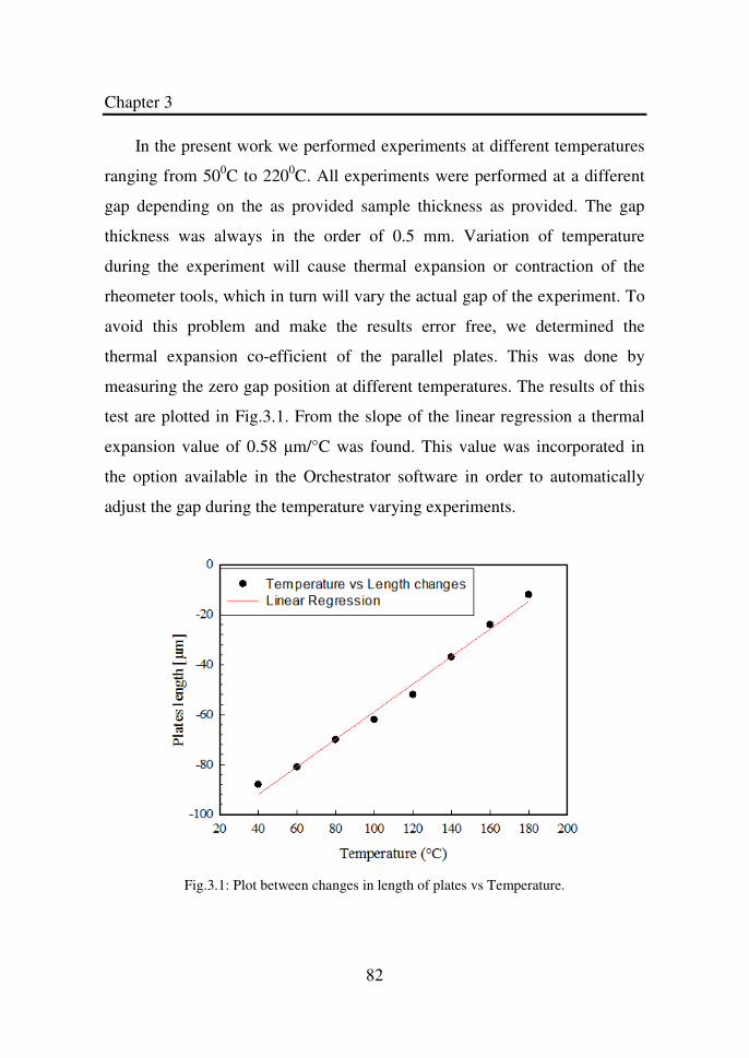
Chapter 3

82

In the present work we performed experiments at different temperatures

ranging from 500C to 2200C. All experiments were performed at a different

gap depending on the as provided sample thickness as provided. The gap

thickness was always in the order of 0.5 mm. Variation of temperature

during the experiment will cause thermal expansion or contraction of the

rheometer tools, which in turn will vary the actual gap of the experiment. To

avoid this problem and make the results error free, we determined the

thermal expansion co-efficient of the parallel plates. This was done by

measuring the zero gap position at different temperatures. The results of this

test are plotted in Fig.3.1. From the slope of the linear regression a thermal

expansion value of 0.58 µm/°C was found. This value was incorporated in

the option available in the Orchestrator software in order to automatically

adjust the gap during the temperature varying experiments.

Fig.3.1: Plot between changes in length of plates vs Temperature.

Chapter 3

83

3.3. Results and Discussion

A first test performed for all samples was a thermal stability test. All

samples were put in the rheometer at 200°C and a constant frequency and

constant strain isothermal annealing was allowed in order to clear the sample

from any crystalline phase and to make sure about thermal stability. During

the annealing the viscoelastic moduli were measured as a function of time.

Two different behaviors were found in this type of experiments. For some

samples, as is the case in Fig. 3.2 for sPP-9, moduli stayed essentially

constant with time, indicating a fast melting and a good thermal stability. For

other samples, such as sPP-3, the transient was longer. In this case, the time

evolution of the moduli shows a continuous increase which eventually levels

off at steady-state conditions after a relatively long time.

The time increase of the moduli is quite unexpected. If crystal melting

were the only phenomenon involved, a decreasing in the moduli would have

been found. An increase of the moduli could be attributed to a residual

reactivity of the samples. This might be due to the presence of catalyst

traces, or to chain crosslinks. Both phenomena would determine an increase

in molecular weight and/or the formation of branched chains, thus resulting

in an increase of the polymer viscoelasticity.

In order to assess the issue of thermal stability the time evolution moduli

data were fitted by a simple exponential growth equation:

G t( ) = G0 + G

∞− G0( ) 1− exp −

t

τ

(3.13)

where G0 is the value at time zero, G∞ is the long time value, and τ is a

characteristic time of the process. An example of the fit is shown in Fig.3.3

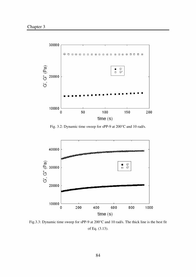
Chapter 3

84

Fig. 3.2: Dynamic time sweep for sPP-9 at 200°C and 10 rad/s.

Fig.3.3: Dynamic time sweep for sPP-9 at 200°C and 10 rad/s. The thick line is the best fit

of Eq. (3.13).

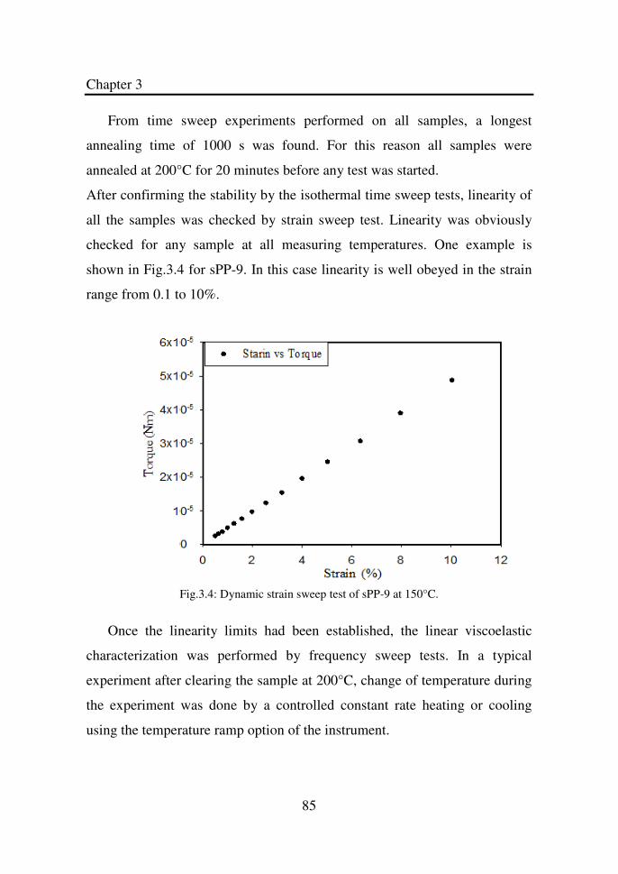
Chapter 3

85

From time sweep experiments performed on all samples, a longest

annealing time of 1000 s was found. For this reason all samples were

annealed at 200°C for 20 minutes before any test was started.

After confirming the stability by the isothermal time sweep tests, linearity of

all the samples was checked by strain sweep test. Linearity was obviously

checked for any sample at all measuring temperatures. One example is

shown in Fig.3.4 for sPP-9. In this case linearity is well obeyed in the strain

range from 0.1 to 10%.

Fig.3.4: Dynamic strain sweep test of sPP-9 at 150°C.

Once the linearity limits had been established, the linear viscoelastic

characterization was performed by frequency sweep tests. In a typical

experiment after clearing the sample at 200°C, change of temperature during

the experiment was done by a controlled constant rate heating or cooling

using the temperature ramp option of the instrument.

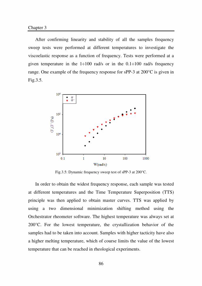
Chapter 3

86

After confirming linearity and stability of all the samples frequency

sweep tests were performed at different temperatures to investigate the

viscoelastic response as a function of frequency. Tests were performed at a

given temperature in the 1÷100 rad/s or in the 0.1÷100 rad/s frequency

range. One example of the frequency response for sPP-3 at 200°C is given in

Fig.3.5.

Fig.3.5: Dynamic frequency sweep test of sPP-3 at 200°C.

In order to obtain the widest frequency response, each sample was tested

at different temperatures and the Time Temperature Superposition (TTS)

principle was then applied to obtain master curves. TTS was applied by

using a two dimensional minimization shifting method using the

Orchestrator rheometer software. The highest temperature was always set at

200°C. For the lowest temperature, the crystallization behavior of the

samples had to be taken into account. Samples with higher tacticity have also

a higher melting temperature, which of course limits the value of the lowest

temperature that can be reached in rheological experiments.

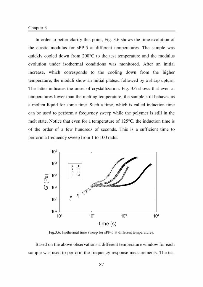
Chapter 3

87

In order to better clarify this point, Fig. 3.6 shows the time evolution of

the elastic modulus for sPP-5 at different temperatures. The sample was

quickly cooled down from 200°C to the test temperature and the modulus

evolution under isothermal conditions was monitored. After an initial

increase, which corresponds to the cooling down from the higher

temperature, the moduli show an initial plateau followed by a sharp upturn.

The latter indicates the onset of crystallization. Fig. 3.6 shows that even at

temperatures lower than the melting temperature, the sample still behaves as

a molten liquid for some time. Such a time, which is called induction time

can be used to perform a frequency sweep while the polymer is still in the

melt state. Notice that even for a temperature of 125°C, the induction time is

of the order of a few hundreds of seconds. This is a sufficient time to

perform a frequency sweep from 1 to 100 rad/s.

Fig.3.6: Isothermal time sweep for sPP-5 at different temperatures.

Based on the above observations a different temperature window for each

sample was used to perform the frequency response measurements. The test

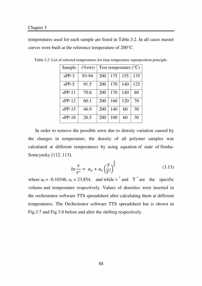
Chapter 3

88

temperatures used for each sample are listed in Table.3.2. In all cases master

curves were built at the reference temperature of 200°C.

Table.3.2: List of selected temperatures for time temperature superposition principle.

Sample (%rrrr) Test temperature (°C)

sPP-3 93-94 200 175 155 135

sPP-5 91.5 200 170 140 125

sPP-11 70.6 200 170 140 80

sPP-12 60.1 200 160 120 70

sPP-15 46.9 200 140 60 30

sPP-18 26.5 200 100 60 30

In order to remove the possible error due to density variation caused by

the changes in temperature, the density of all polymer samples was

calculated at different temperatures by using equation of state of Simha-

Somcynsky [112, 113].

) **∗ =, + ∗

-.

(3.13)

where a0 = -0.10346, a1 = 23,854, and while v * and T * are the specific

volume and temperature respectively. Values of densities were inserted in

the orchestrator software TTS spreadsheet after calculating them at different

temperatures. The Orchestrator software TTS spreadsheet bar is shown in

Fig.3.7 and Fig.3.8 before and after the shifting respectively.

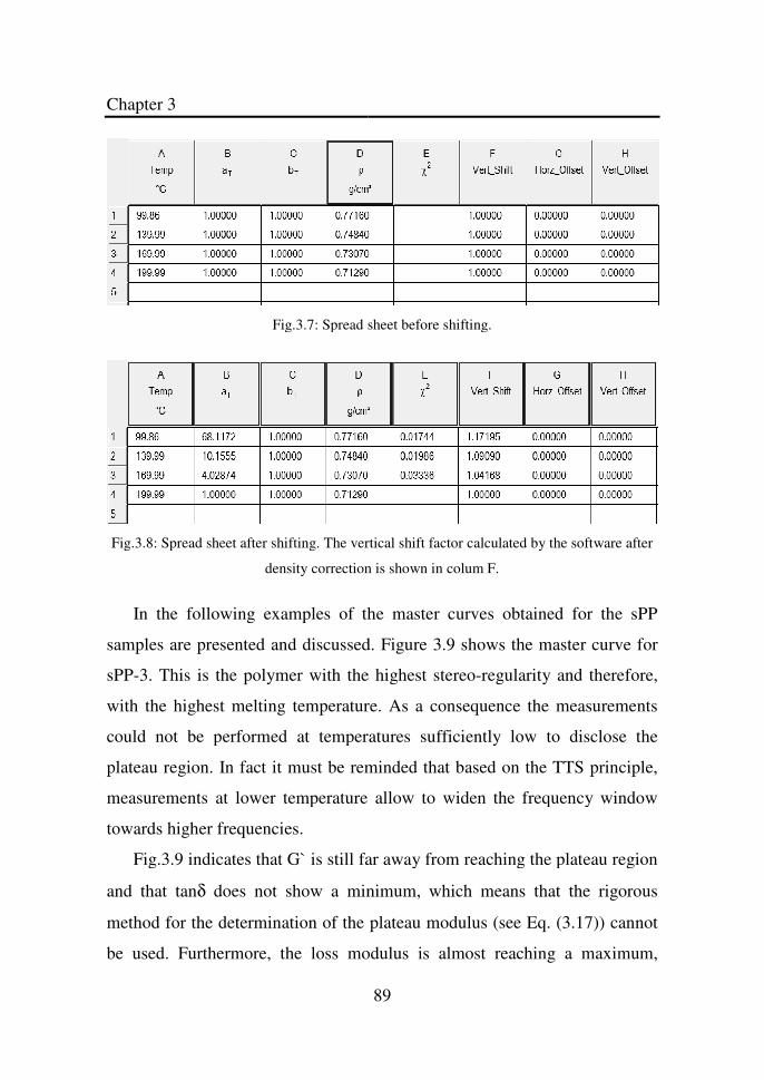
Chapter 3

Fig.3.7: Spread sheet before shifting.

Fig.3.8: Spread sheet after shifting. The vertical shift factor calculated by the software

density correction is shown in colum F.

In the following examples of the master curves obtained for the sPP

samples are presented and discussed. Figure 3.9 shows the master curve for

sPP-3. This is the polymer with the highest stereo

with the highest melting temperature. As a consequence

could not be performed at temperatures sufficiently low to disclose the

plateau region. In fact it must be reminded that

measurements at lower temperature allow to widen the frequency window

towards higher frequencies.

Fig.3.9 indicates that G` is still far away from reaching the plateau region

and that tanδ does not show a minimum, which means that the rigorous

method for the determination of the

be used. Furthermore, the loss modulus is almost reaching a maximum,

89

Fig.3.7: Spread sheet before shifting.

Fig.3.8: Spread sheet after shifting. The vertical shift factor calculated by the software after

density correction is shown in colum F.

In the following examples of the master curves obtained for the sPP

samples are presented and discussed. Figure 3.9 shows the master curve for

e highest stereo-regularity and therefore,

g temperature. As a consequence the measurements

could not be performed at temperatures sufficiently low to disclose the

it must be reminded that based on the TTS principle,

mperature allow to widen the frequency window

Fig.3.9 indicates that G` is still far away from reaching the plateau region

does not show a minimum, which means that the rigorous

method for the determination of the plateau modulus (see Eq. (3.17)) cannot

be used. Furthermore, the loss modulus is almost reaching a maximum,

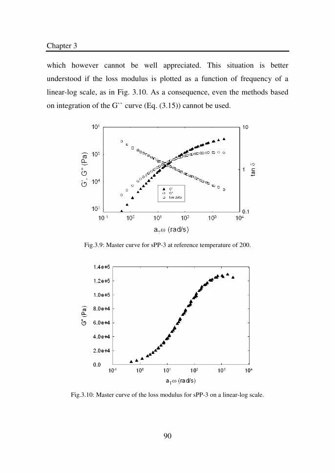
Chapter 3

90

which however cannot be well appreciated. This situation is better

understood if the loss modulus is plotted as a function of frequency of a

linear-log scale, as in Fig. 3.10. As a consequence, even the methods based

on integration of the G`` curve (Eq. (3.15)) cannot be used.

Fig.3.9: Master curve for sPP-3 at reference temperature of 200.

Fig.3.10: Master curve of the loss modulus for sPP-3 on a linear-log scale.

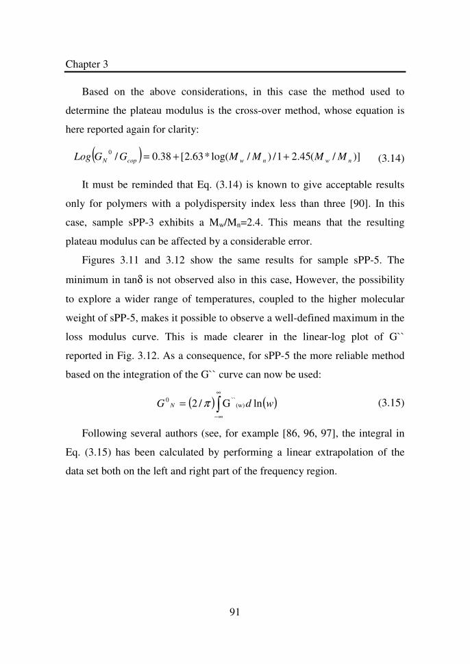
Chapter 3

91

Based on the above considerations, in this case the method used to

determine the plateau modulus is the cross-over method, whose equation is

here reported again for clarity:

( ) )]/(45.21/)/log(*63.2[38.0/0nwnwcopN MMMMGGLog ++=

(3.14)

It must be reminded that Eq. (3.14) is known to give acceptable results

only for polymers with a polydispersity index less than three [90]. In this

case, sample sPP-3 exhibits a Mw/Mn=2.4. This means that the resulting

plateau modulus can be affected by a considerable error.

Figures 3.11 and 3.12 show the same results for sample sPP-5. The

minimum in tanδ is not observed also in this case, However, the possibility

to explore a wider range of temperatures, coupled to the higher molecular

weight of sPP-5, makes it possible to observe a well-defined maximum in the

loss modulus curve. This is made clearer in the linear-log plot of G``

reported in Fig. 3.12. As a consequence, for sPP-5 the more reliable method

based on the integration of the G`` curve can now be used:

( ) ( )wdG N lnG/2 (w)``0

∫∞

∞−

= π

(3.15)

Following several authors (see, for example [86, 96, 97], the integral in

Eq. (3.15) has been calculated by performing a linear extrapolation of the

data set both on the left and right part of the frequency region.

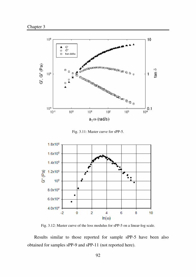
Chapter 3

92

Fig. 3.11: Master curve for sPP-5.

Fig. 3.12: Master curve of the loss modulus for sPP-5 on a linear-log scale.

Results similar to those reported for sample sPP-5 have been also

obtained for samples sPP-9 and sPP-11 (not reported here).

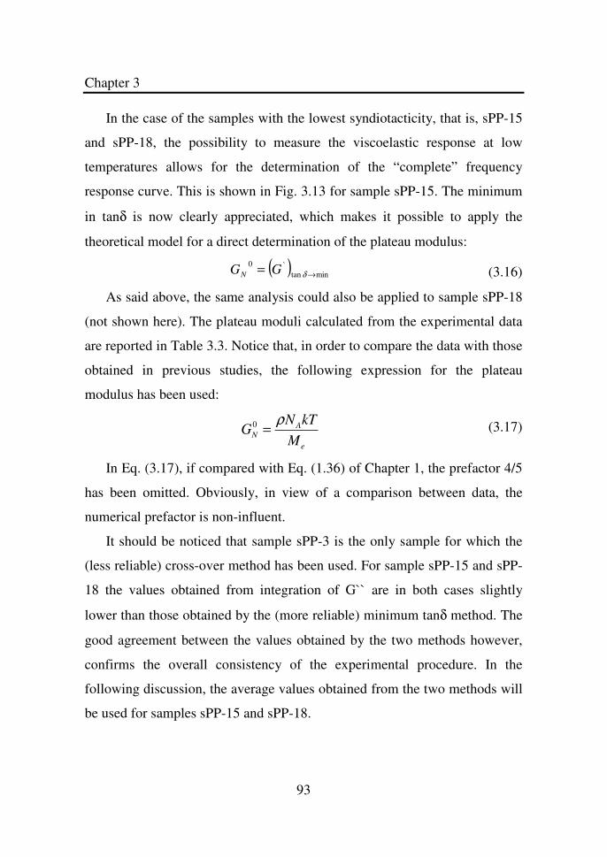
Chapter 3

93

In the case of the samples with the lowest syndiotacticity, that is, sPP-15

and sPP-18, the possibility to measure the viscoelastic response at low

temperatures allows for the determination of the “complete” frequency

response curve. This is shown in Fig. 3.13 for sample sPP-15. The minimum

in tanδ is now clearly appreciated, which makes it possible to apply the

theoretical model for a direct determination of the plateau modulus:

( ) mintan`0

→= δGGN

(3.16)

As said above, the same analysis could also be applied to sample sPP-18

(not shown here). The plateau moduli calculated from the experimental data

are reported in Table 3.3. Notice that, in order to compare the data with those

obtained in previous studies, the following expression for the plateau

modulus has been used:

GN

0 =ρNAkT

Me

(3.17)

In Eq. (3.17), if compared with Eq. (1.36) of Chapter 1, the prefactor 4/5

has been omitted. Obviously, in view of a comparison between data, the

numerical prefactor is non-influent.

It should be noticed that sample sPP-3 is the only sample for which the

(less reliable) cross-over method has been used. For sample sPP-15 and sPP-

18 the values obtained from integration of G`` are in both cases slightly

lower than those obtained by the (more reliable) minimum tanδ method. The

good agreement between the values obtained by the two methods however,

confirms the overall consistency of the experimental procedure. In the

following discussion, the average values obtained from the two methods will

be used for samples sPP-15 and sPP-18.

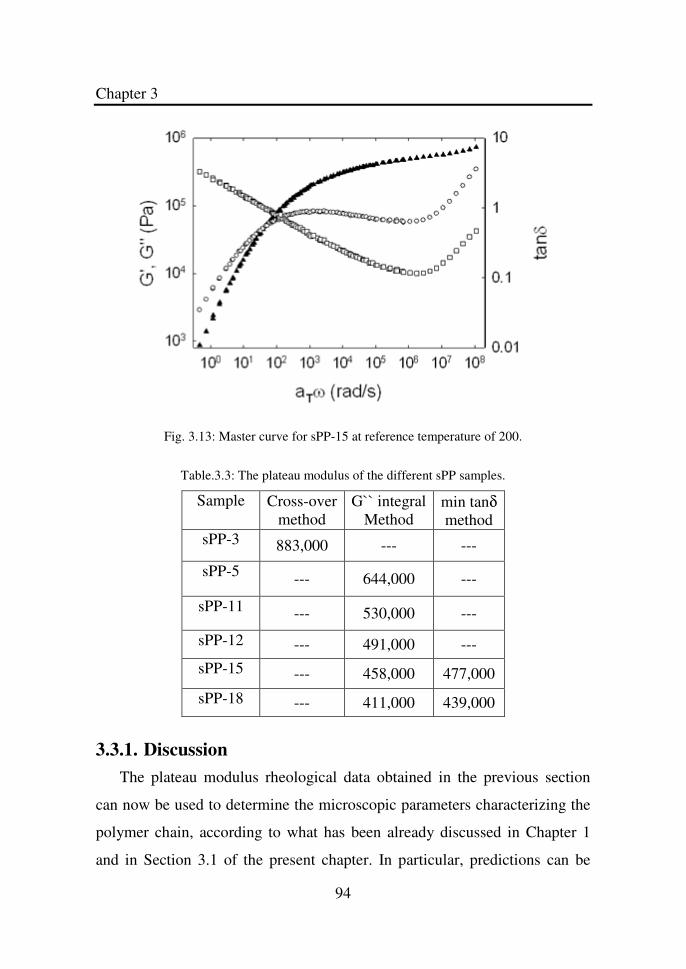
Chapter 3

94

Fig. 3.13: Master curve for sPP-15 at reference temperature of 200.

Table.3.3: The plateau modulus of the different sPP samples.

Sample Cross-over method

G`` integral Method

min tanδ method

sPP-3 883,000 --- ---

sPP-5 --- 644,000 ---

sPP-11 --- 530,000 ---

sPP-12 --- 491,000 ---

sPP-15 --- 458,000 477,000

sPP-18 --- 411,000 439,000

3.3.1. Discussion

The plateau modulus rheological data obtained in the previous section

can now be used to determine the microscopic parameters characterizing the

polymer chain, according to what has been already discussed in Chapter 1

and in Section 3.1 of the present chapter. In particular, predictions can be

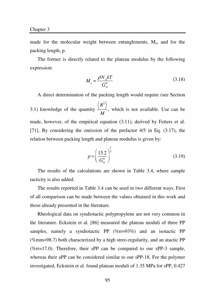
Chapter 3

95

made for the molecular weight between entanglements, Me, and for the

packing length, p.

The former is directly related to the plateau modulus by the following

expression:

M

e=

ρNAkT

GN

0

(3.18)

A direct determination of the packing length would require (see Section

3.1) knowledge of the quantity

R2

M, which is not available. Use can be

made, however, of the empirical equation (3.11), derived by Fetters et al.

[71]. By considering the omission of the prefactor 4/5 in Eq. (3.17), the

relation between packing length and plateau modulus is given by:

p =15.2

GN

0

13

(3.19)

The results of the calculations are shown in Table 3.4, where sample

tacticity is also added.

The results reported in Table 3.4 can be used in two different ways. First

of all comparison can be made between the values obtained in this work and

those already presented in the literature.

Rheological data on syndiotactic polypropylene are not very common in

the literature. Eckstein et al. [86] measured the plateau moduli of three PP

samples, namely a syndiotactic PP (%rr=93%) and an isotactic PP

(%mm=98.7) both characterized by a high streo-regularity, and an atactic PP

(%rr=17.0). Therefore, their sPP can be compared to our sPP-3 sample,

whereas their aPP can be considered similar to our sPP-18. For the polymer

investigated, Eckstein et al. found plateau moduli of 1.35 MPa for sPP, 0.427

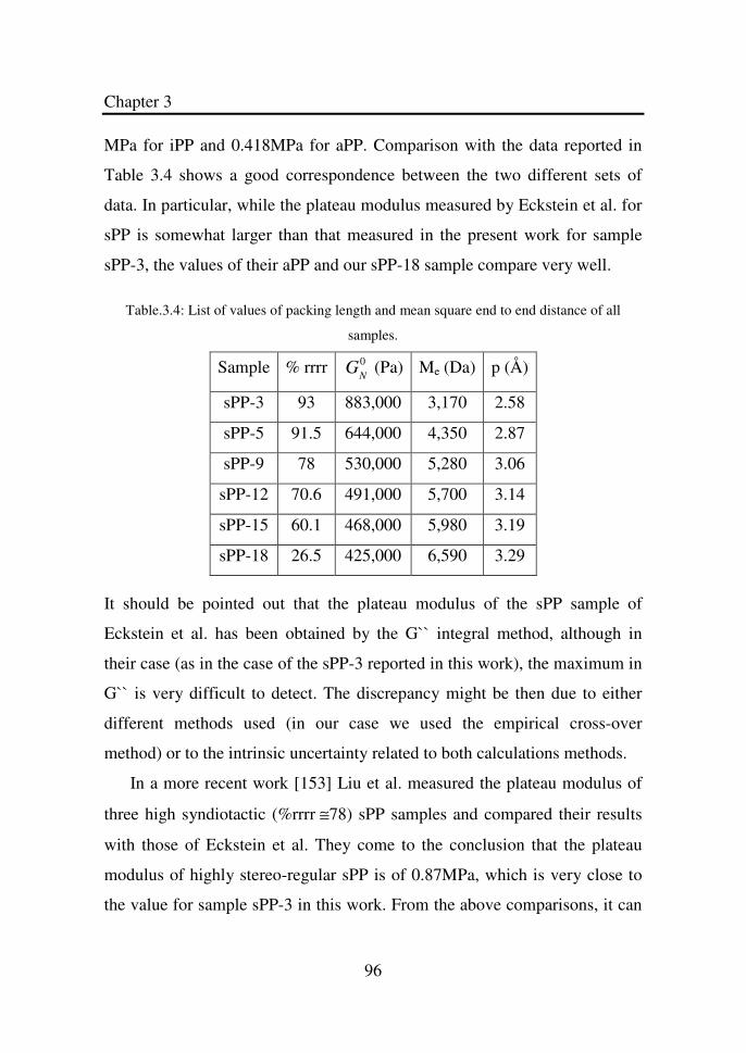
Chapter 3

96

MPa for iPP and 0.418MPa for aPP. Comparison with the data reported in

Table 3.4 shows a good correspondence between the two different sets of

data. In particular, while the plateau modulus measured by Eckstein et al. for

sPP is somewhat larger than that measured in the present work for sample

sPP-3, the values of their aPP and our sPP-18 sample compare very well.

Table.3.4: List of values of packing length and mean square end to end distance of all

samples.

Sample % rrrr GN

0 (Pa) Me (Da) p (Å)

sPP-3 93 883,000 3,170 2.58

sPP-5 91.5 644,000 4,350 2.87

sPP-9 78 530,000 5,280 3.06

sPP-12 70.6 491,000 5,700 3.14

sPP-15 60.1 468,000 5,980 3.19

sPP-18 26.5 425,000 6,590 3.29

It should be pointed out that the plateau modulus of the sPP sample of

Eckstein et al. has been obtained by the G`` integral method, although in

their case (as in the case of the sPP-3 reported in this work), the maximum in

G`` is very difficult to detect. The discrepancy might be then due to either

different methods used (in our case we used the empirical cross-over

method) or to the intrinsic uncertainty related to both calculations methods.

In a more recent work [153] Liu et al. measured the plateau modulus of

three high syndiotactic (%rrrr ≅78) sPP samples and compared their results

with those of Eckstein et al. They come to the conclusion that the plateau

modulus of highly stereo-regular sPP is of 0.87MPa, which is very close to

the value for sample sPP-3 in this work. From the above comparisons, it can

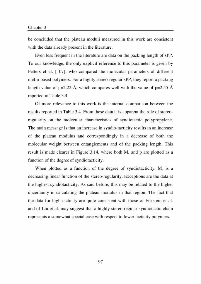
Chapter 3

97

be concluded that the plateau moduli measured in this work are consistent

with the data already present in the literature.

Even less frequent in the literature are data on the packing length of sPP.

To our knowledge, the only explicit reference to this parameter is given by

Fetters et al. [107], who compared the molecular parameters of different

olefin-based polymers. For a highly stereo-regular sPP, they report a packing

length value of p=2.22 Å, which compares well with the value of p=2.55 Å

reported in Table 3.4.

Of more relevance to this work is the internal comparison between the

results reported in Table 3.4. From these data it is apparent the role of stereo-

regularity on the molecular characteristics of syndiotactic polypropylene.

The main message is that an increase in syndio-tacticity results in an increase

of the plateau modulus and correspondingly in a decrease of both the

molecular weight between entanglements and of the packing length. This

result is made clearer in Figure 3.14, where both Me and p are plotted as a

function of the degree of syndiotacticity.

When plotted as a function of the degree of syndiotacticity, Me is a

decreasing linear function of the stereo-regularity. Exceptions are the data at

the highest syndiotacticity. As said before, this may be related to the higher

uncertainty in calculating the plateau modulus in that region. The fact that

the data for high tacticity are quite consistent with those of Eckstein et al.

and of Liu et al. may suggest that a highly stereo-regular syndiotactic chain

represents a somewhat special case with respect to lower tacticity polymers.

Chapter 3

98

Fig. 3.14: The molecular weight between entanglements and the packing length as a function

of the degree of tacticity. The straight line is drawn through the Me data just to guide the

eye.

In terms of interrelations between molecular architecture and

microscopic properties, the data suggest the following scenario. For high

degrees of syndiotacticity polymer chains "fill" the available space in a more

efficient way than either lower syndiotacticity or atactic/isotactic chains.

This is confirmed by the lower value of the packing length at high rrrr

values, meaning that isotactic and atactic polymers are "bulkier" than the

more syndiotactic ones. This might be explained by the alternate disposition

of the side methyl group along the PP backbone. It is reasonable that such a

disposition generates a better packing of the chain units even with respect to

the isotactic arrangement, where the methyl group placed on the same side of

the chain may form a closer sequence of side groups, giving raise to larger

repulsion effects.

Chapter 3

99

3.4. Concluding Remarks

The linear viscoelastic measurements performed on sPPs of different

stereoregularity show that the plateau modulus and therefore the molecular

weight between entanglements significantly depend upon on the degree of

syndiotacticity of the polymer chain. In particular it was shown that Me, as

well as the packing length decreases with increase in the degree of

syndiotacticity.

It is also verified that viscoelasticity is sensitive to chain parameters and

can be used to predict it.

The results demonstrate that viscoelasticity is a powerful tool determines

the local details of the molecular architecture and chain parameters of the

crystalline elastomers.

Chapter 4

100

Quiscent Crystallization of Syndiotactic

Polypropylenes

4.1. Introduction

Crystallization of polymers is a process associated with the partial

alignment of the molecular chains. These chains fold together and form

ordered regions called lamella, which compose larger spheroidal structures

named spherulites. From thermodynamic consideration alone, a crystal is at

lower energy state than the liquid when the temperature is below the melting

point, while at melting point a condition of equilibrium exists between the

crystal and the liquid as both phases have the same value of free energy (G)

and ∆G = 0 [109]. For the isothermal process such as fusion at Tm , ∆Gf = 0.

/ = /0 − /1 (4.1)

At Tm /0 − /1 = 0 (4.2)

/0 = TΔS (4.3)

6 = /0//1 (4.4)

Thus both the enthalpic and entropic effects will determine the

equilibrium melting point temperature of any crystalline polymer.

During the last decades, the use of rheological techniques to examine

polymer crystallization has got increasing importance. When cooled below

thermodynamic melting temperature, crystalline polymers undergo

crystallization. The early stages of this process are characterized by the

gradual change in the mechanical response of the material from the liquid to

the solid, which is due to the microstructure evolution of the system. This is

Chapter 4

101

one of the great features of the rheological technique, which distinguishes it

from the traditional DSC technique.

The main advantage of rheological technique, over traditional ones such

as DSC, is that they can be more sensitive when crystallization kinetics are

slow [12] and can provide information on the morphology of the

crystallizing material [149]. On the other hand, the major drawback in the

use of rheological techniques is that a universal correlation between

viscoelastic properties and crystallinity is still missing. And also rheometry

is unable to analyze the crystallization process when the crystallization

kinetics are very fast. In this case DSC is the better candidate for the study of

crystallization kinetics. To overcome these limitations, Kiewit et al. [150]

have recently combined a rheometer and a DSC into a single instrument to

compare the evolution of rheological properties to crystallinity as measured

from heat flow integration. While this RheoDSC instrument was shown to

provide reliable measurements, a systematic study on crystallizing systems is

still missing.

Rheological functions can be used to calculate the evolution of relative

crystallinity, x(t), once a functional relation is assumed. Khanna [88], for

example, suggested a linear relation between elastic modulus and

crystallinity and used this idea to study the crystallization kinetics of

different, nucleated and un-nucleated, polymers.

' ' ' '0 0( ) /x t G G G G∞= − − (4.5)

where x(t) = Relative crystallinity, G`0 = Initial plateau value of elastic

modulus, 'G ∞ = Final plateau value of elastic modulus and '

G = Elastic

modulus at all points

Polymer crystallization is a complex phenomenon that affects the final

properties of processed polymeric materials. The quality and quantity of

Chapter 4

102

crystallization, i.e., the number, size, shape, and crystalline form of the

crystallites depend upon on a number of different parameters like molecular

weight, polydispersity and tacticity of the polymer system under

consideration [151]. Among all tacticity is one of the important factors,

which affects the crystallization process.

The aim of the present work is to study the quiescent crystallization

behavior of a series of syndiotactic polypropylenes of different degrees of

syndiotacticity by coupling rheological method to more conventional

technique (Differential Scanning Calorimetry) and to relate the

crystallization behavior to the syndiotacticity of the syndiotactic

polypropylene chain.


4.2.1. Material

Samples of sPP with different degrees of syndiotacticity were used for

the crystallization study. The relevant properties of the polymers are reported

in Table 4.1. The samples labelled sPP-8 and sPP-5 are commercial

polymers (supplied by Montell Technology). The others come from

laboratory synthesis using metallocene catalysts [44-50]. It can be noted

from Table4.1 that samples are characterized by varying degrees of

syndiotacticity (%rrrr), melting temperature (Tm) and molecular weight

distribution.

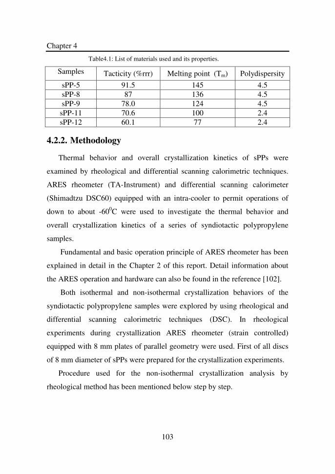
Chapter 4

103

Table4.1: List of materials used and its properties.

Samples Tacticity (%rrr) Melting point (Tm) Polydispersity

sPP-5 91.5 145 4.5 sPP-8 87 136 4.5 sPP-9 78.0 124 4.5

sPP-11 70.6 100 2.4 sPP-12 60.1 77 2.4

4.2.2. Methodology

Thermal behavior and overall crystallization kinetics of sPPs were

examined by rheological and differential scanning calorimetric techniques.

ARES rheometer (TA-Instrument) and differential scanning calorimeter

(Shimadtzu DSC60) equipped with an intra-cooler to permit operations of

down to about -600C were used to investigate the thermal behavior and

overall crystallization kinetics of a series of syndiotactic polypropylene

samples.

Fundamental and basic operation principle of ARES rheometer has been

explained in detail in the Chapter 2 of this report. Detail information about

the ARES operation and hardware can also be found in the reference [102].

Both isothermal and non-isothermal crystallization behaviors of the

syndiotactic polypropylene samples were explored by using rheological and

differential scanning calorimetric techniques (DSC). In rheological

experiments during crystallization ARES rheometer (strain controlled)

equipped with 8 mm plates of parallel geometry were used. First of all discs

of 8 mm diameter of sPPs were prepared for the crystallization experiments.

Procedure used for the non-isothermal crystallization analysis by

rheological method has been mentioned below step by step.

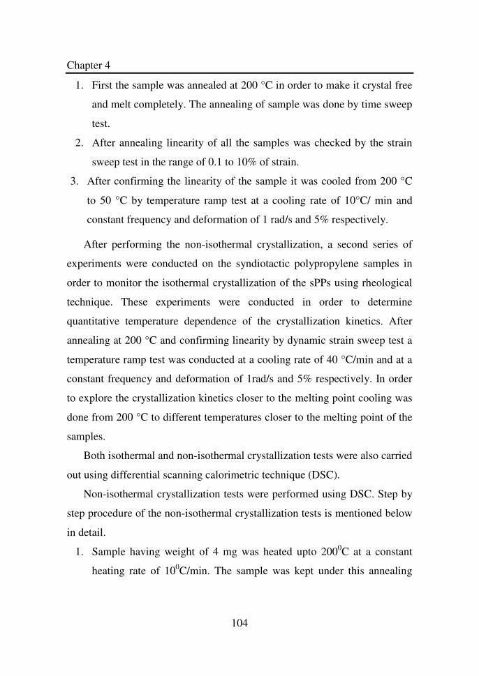
Chapter 4

104

1. First the sample was annealed at 200 °C in order to make it crystal free

and melt completely. The annealing of sample was done by time sweep

test.

2. After annealing linearity of all the samples was checked by the strain

sweep test in the range of 0.1 to 10% of strain.

3. After confirming the linearity of the sample it was cooled from 200 °C

to 50 °C by temperature ramp test at a cooling rate of 10°C/ min and

constant frequency and deformation of 1 rad/s and 5% respectively.

After performing the non-isothermal crystallization, a second series of

experiments were conducted on the syndiotactic polypropylene samples in

order to monitor the isothermal crystallization of the sPPs using rheological

technique. These experiments were conducted in order to determine

quantitative temperature dependence of the crystallization kinetics. After

annealing at 200 °C and confirming linearity by dynamic strain sweep test a

temperature ramp test was conducted at a cooling rate of 40 °C/min and at a

constant frequency and deformation of 1rad/s and 5% respectively. In order

to explore the crystallization kinetics closer to the melting point cooling was

done from 200 °C to different temperatures closer to the melting point of the

samples.

Both isothermal and non-isothermal crystallization tests were also carried

out using differential scanning calorimetric technique (DSC).

Non-isothermal crystallization tests were performed using DSC. Step by

step procedure of the non-isothermal crystallization tests is mentioned below

in detail.

1. Sample having weight of 4 mg was heated upto 2000C at a constant

heating rate of 100C/min. The sample was kept under this annealing

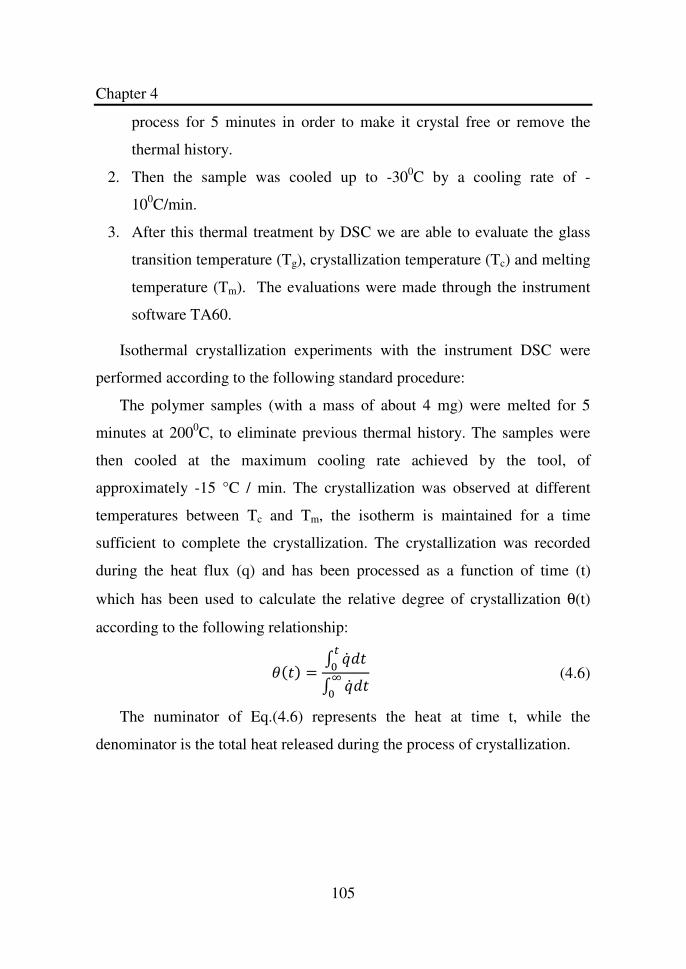
Chapter 4

105

process for 5 minutes in order to make it crystal free or remove the

thermal history.

2. Then the sample was cooled up to -300C by a cooling rate of -

100C/min.

3. After this thermal treatment by DSC we are able to evaluate the glass

transition temperature (Tg), crystallization temperature (Tc) and melting

temperature (Tm). The evaluations were made through the instrument

software TA60.

Isothermal crystallization experiments with the instrument DSC were

performed according to the following standard procedure:

The polymer samples (with a mass of about 4 mg) were melted for 5

minutes at 2000C, to eliminate previous thermal history. The samples were

then cooled at the maximum cooling rate achieved by the tool, of

approximately -15 °C / min. The crystallization was observed at different

temperatures between Tc and Tm, the isotherm is maintained for a time

sufficient to complete the crystallization. The crystallization was recorded

during the heat flux (q) and has been processed as a function of time (t)

which has been used to calculate the relative degree of crystallization θ(t)

according to the following relationship:

78 = 9 # :8;

9 # :8<

(4.6)

The numinator of Eq.(4.6) represents the heat at time t, while the

denominator is the total heat released during the process of crystallization.

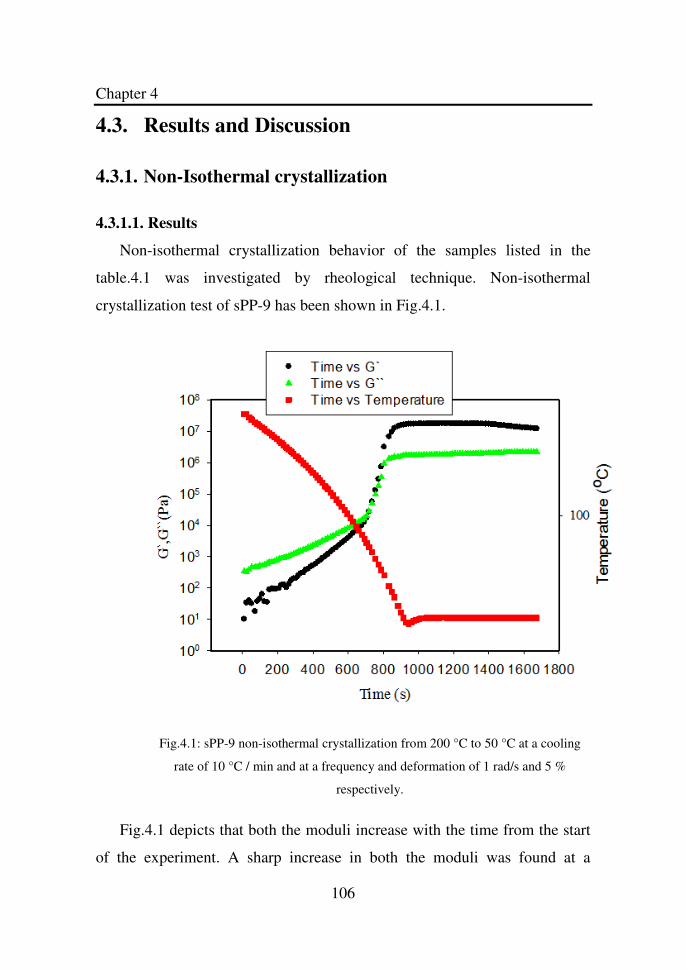
Chapter 4

106


4.3.1. Non-Isothermal crystallization

4.3.1.1. Results

Non-isothermal crystallization behavior of the samples listed in the

table.4.1 was investigated by rheological technique. Non-isothermal

crystallization test of sPP-9 has been shown in Fig.4.1.

Fig.4.1: sPP-9 non-isothermal crystallization from 200 °C to 50 °C at a cooling

rate of 10 °C / min and at a frequency and deformation of 1 rad/s and 5 %

respectively.

Fig.4.1 depicts that both the moduli increase with the time from the start

of the experiment. A sharp increase in both the moduli was found at a

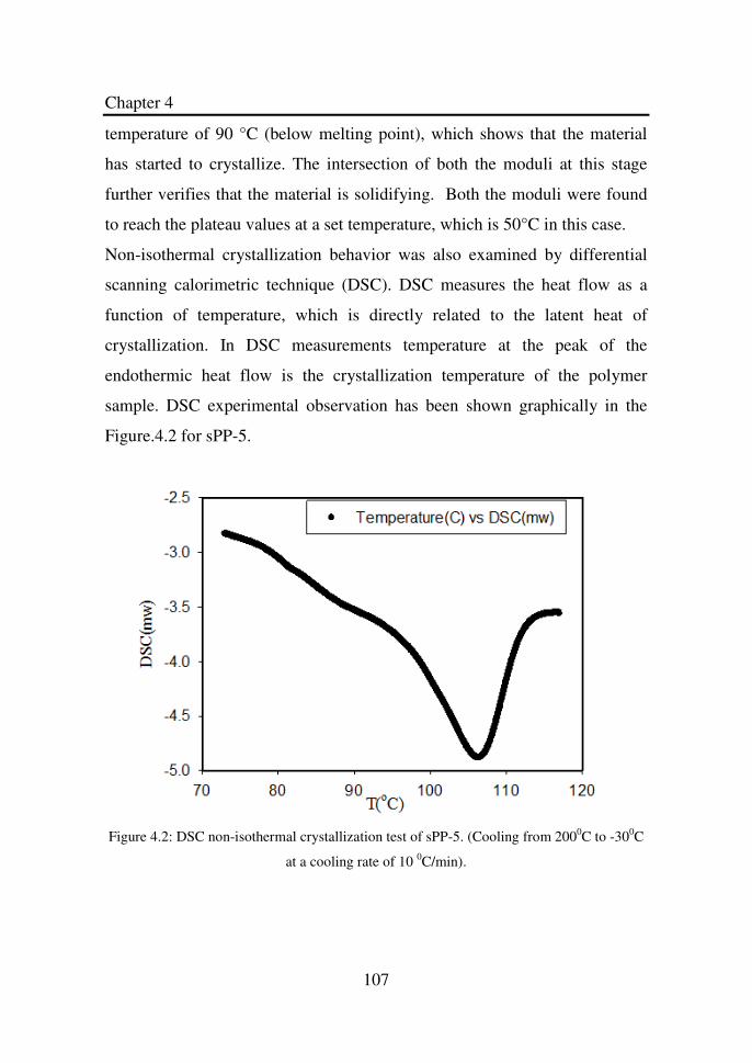
Chapter 4

107

temperature of 90 °C (below melting point), which shows that the material

has started to crystallize. The intersection of both the moduli at this stage

further verifies that the material is solidifying. Both the moduli were found

to reach the plateau values at a set temperature, which is 50°C in this case.

Non-isothermal crystallization behavior was also examined by differential

scanning calorimetric technique (DSC). DSC measures the heat flow as a

function of temperature, which is directly related to the latent heat of

crystallization. In DSC measurements temperature at the peak of the

endothermic heat flow is the crystallization temperature of the polymer

sample. DSC experimental observation has been shown graphically in the

Figure.4.2 for sPP-5.

Figure 4.2: DSC non-isothermal crystallization test of sPP-5. (Cooling from 2000C to -300C

at a cooling rate of 10 0C/min).

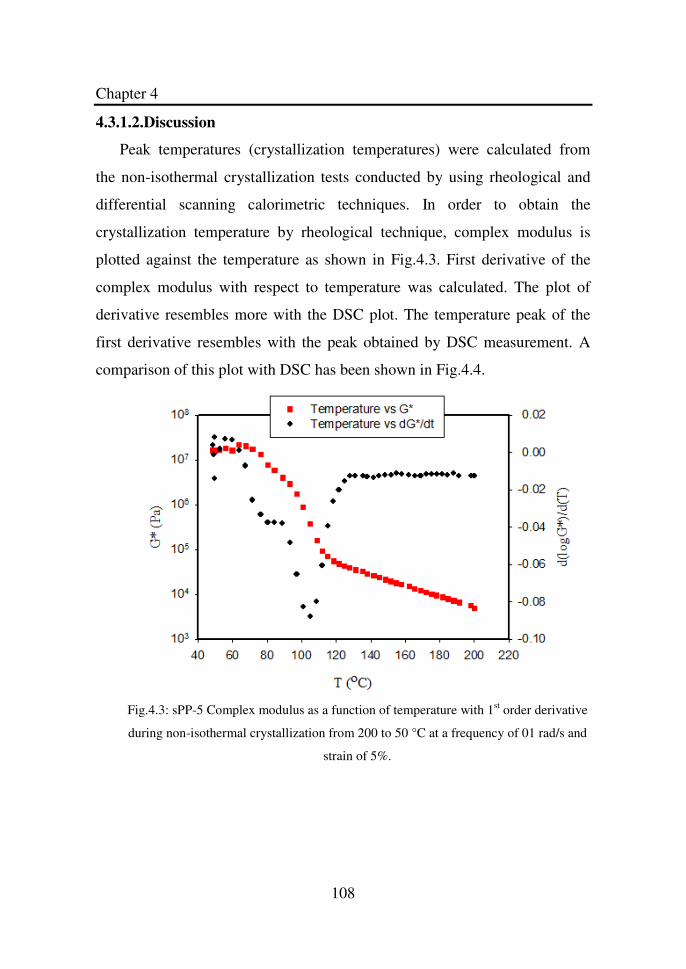
Chapter 4

108

4.3.1.2.Discussion

Peak temperatures (crystallization temperatures) were calculated from

the non-isothermal crystallization tests conducted by using rheological and

differential scanning calorimetric techniques. In order to obtain the

crystallization temperature by rheological technique, complex modulus is

plotted against the temperature as shown in Fig.4.3. First derivative of the

complex modulus with respect to temperature was calculated. The plot of

derivative resembles more with the DSC plot. The temperature peak of the

first derivative resembles with the peak obtained by DSC measurement. A

comparison of this plot with DSC has been shown in Fig.4.4.

Fig.4.3: sPP-5 Complex modulus as a function of temperature with 1st order derivative

during non-isothermal crystallization from 200 to 50 °C at a frequency of 01 rad/s and

strain of 5%.

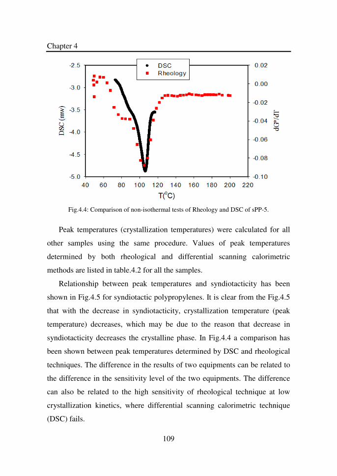
Chapter 4

109

Fig.4.4: Comparison of non-isothermal tests of Rheology and DSC of sPP-5.

Peak temperatures (crystallization temperatures) were calculated for all

other samples using the same procedure. Values of peak temperatures

determined by both rheological and differential scanning calorimetric

methods are listed in table.4.2 for all the samples.

Relationship between peak temperatures and syndiotacticity has been

shown in Fig.4.5 for syndiotactic polypropylenes. It is clear from the Fig.4.5

that with the decrease in syndiotacticity, crystallization temperature (peak

temperature) decreases, which may be due to the reason that decrease in

syndiotacticity decreases the crystalline phase. In Fig.4.4 a comparison has

been shown between peak temperatures determined by DSC and rheological

techniques. The difference in the results of two equipments can be related to

the difference in the sensitivity level of the two equipments. The difference

can also be related to the high sensitivity of rheological technique at low

crystallization kinetics, where differential scanning calorimetric technique

(DSC) fails.

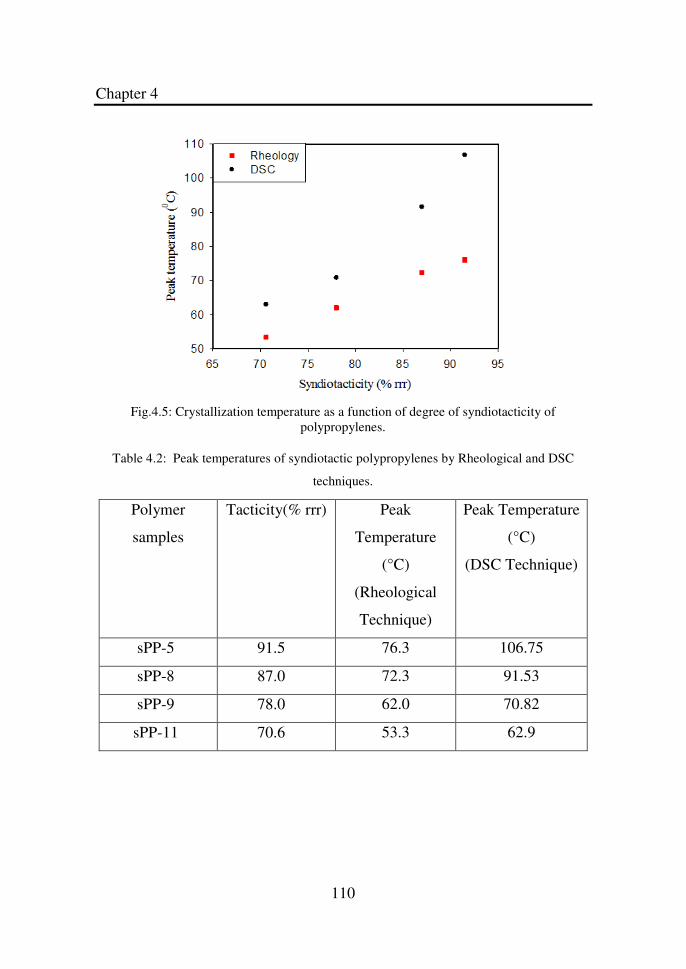
Chapter 4

110

Fig.4.5: Crystallization temperature as a function of degree of syndiotacticity of

polypropylenes.

Table 4.2: Peak temperatures of syndiotactic polypropylenes by Rheological and DSC

techniques.

Polymer

samples

Tacticity(% rrr) Peak

Temperature

(°C)

(Rheological

Technique)

Peak Temperature

(°C)

(DSC Technique)

sPP-5 91.5 76.3 106.75

sPP-8 87.0 72.3 91.53

sPP-9 78.0 62.0 70.82

sPP-11 70.6 53.3 62.9

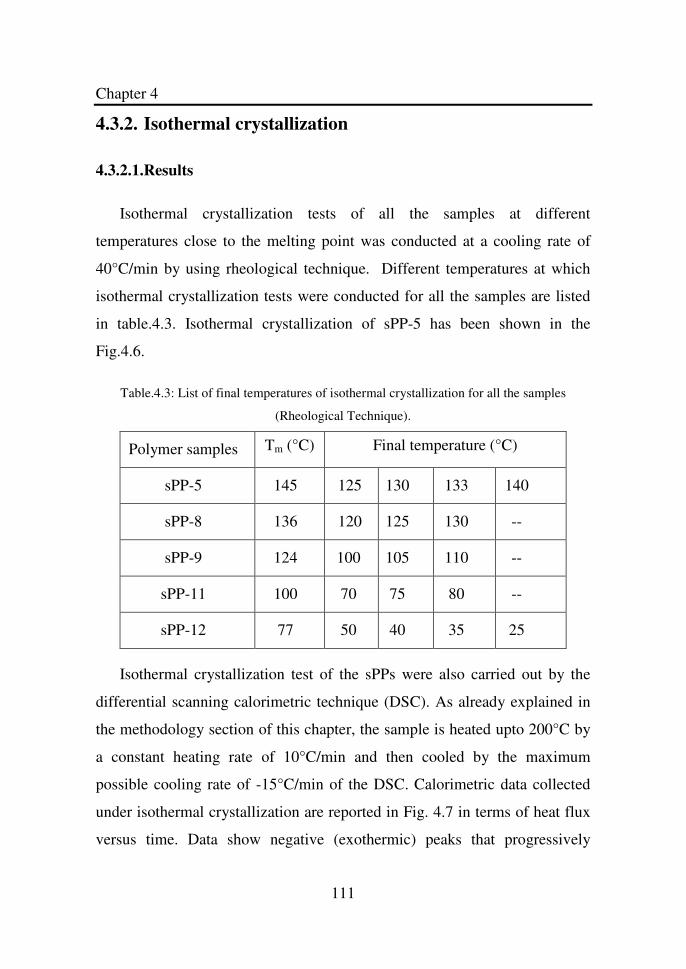
Chapter 4

111

4.3.2. Isothermal crystallization

4.3.2.1.Results

Isothermal crystallization tests of all the samples at different

temperatures close to the melting point was conducted at a cooling rate of

40°C/min by using rheological technique. Different temperatures at which

isothermal crystallization tests were conducted for all the samples are listed

in table.4.3. Isothermal crystallization of sPP-5 has been shown in the

Fig.4.6.

Table.4.3: List of final temperatures of isothermal crystallization for all the samples

(Rheological Technique).

Polymer samples Tm (°C) Final temperature (°C)

sPP-5 145 125 130 133 140

sPP-8 136 120 125 130 --

sPP-9 124 100 105 110 --

sPP-11 100 70 75 80 --

sPP-12 77 50 40 35 25

Isothermal crystallization test of the sPPs were also carried out by the

differential scanning calorimetric technique (DSC). As already explained in

the methodology section of this chapter, the sample is heated upto 200°C by

a constant heating rate of 10°C/min and then cooled by the maximum

possible cooling rate of -15°C/min of the DSC. Calorimetric data collected

under isothermal crystallization are reported in Fig. 4.7 in terms of heat flux

versus time. Data show negative (exothermic) peaks that progressively

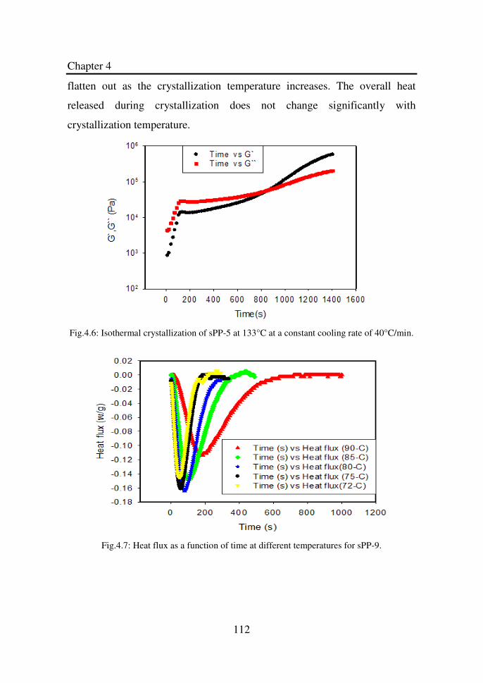
Chapter 4

112

flatten out as the crystallization temperature increases. The overall heat

released during crystallization does not change significantly with

crystallization temperature.

Fig.4.6: Isothermal crystallization of sPP-5 at 133°C at a constant cooling rate of 40°C/min.

Fig.4.7: Heat flux as a function of time at different temperatures for sPP-9.

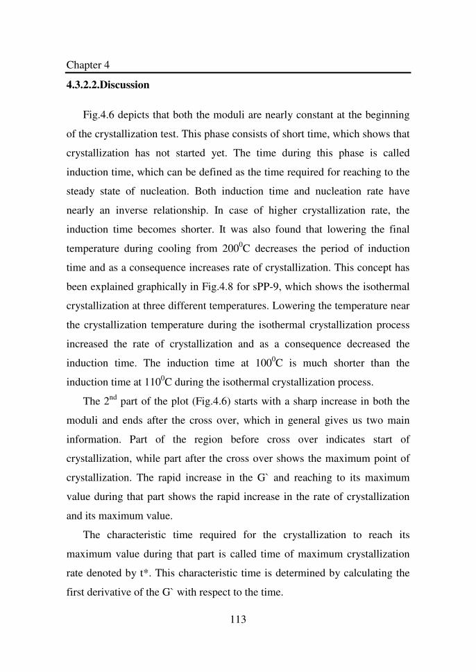
Chapter 4

113

4.3.2.2.Discussion

Fig.4.6 depicts that both the moduli are nearly constant at the beginning

of the crystallization test. This phase consists of short time, which shows that

crystallization has not started yet. The time during this phase is called

induction time, which can be defined as the time required for reaching to the

steady state of nucleation. Both induction time and nucleation rate have

nearly an inverse relationship. In case of higher crystallization rate, the

induction time becomes shorter. It was also found that lowering the final

temperature during cooling from 2000C decreases the period of induction

time and as a consequence increases rate of crystallization. This concept has

been explained graphically in Fig.4.8 for sPP-9, which shows the isothermal

crystallization at three different temperatures. Lowering the temperature near

the crystallization temperature during the isothermal crystallization process

increased the rate of crystallization and as a consequence decreased the

induction time. The induction time at 1000C is much shorter than the

induction time at 1100C during the isothermal crystallization process.

The 2nd part of the plot (Fig.4.6) starts with a sharp increase in both the

moduli and ends after the cross over, which in general gives us two main

information. Part of the region before cross over indicates start of

crystallization, while part after the cross over shows the maximum point of

crystallization. The rapid increase in the G` and reaching to its maximum

value during that part shows the rapid increase in the rate of crystallization

and its maximum value.

The characteristic time required for the crystallization to reach its

maximum value during that part is called time of maximum crystallization

rate denoted by t*. This characteristic time is determined by calculating the

first derivative of the G` with respect to the time.

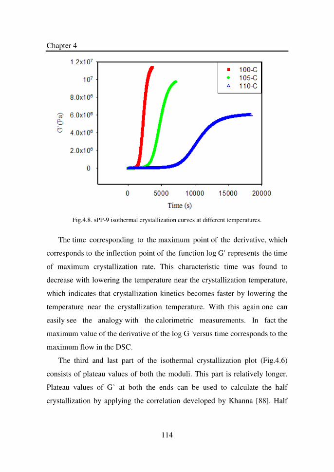
Chapter 4

114

Fig.4.8. sPP-9 isothermal crystallization curves at different temperatures.

The time corresponding to the maximum point of the derivative, which

corresponds to the inflection point of the function log G' represents the time

of maximum crystallization rate. This characteristic time was found to

decrease with lowering the temperature near the crystallization temperature,

which indicates that crystallization kinetics becomes faster by lowering the

temperature near the crystallization temperature. With this again one can

easily see the analogy with the calorimetric measurements. In fact the

maximum value of the derivative of the log G 'versus time corresponds to the

maximum flow in the DSC.

The third and last part of the isothermal crystallization plot (Fig.4.6)

consists of plateau values of both the moduli. This part is relatively longer.

Plateau values of G` at both the ends can be used to calculate the half

crystallization by applying the correlation developed by Khanna [88]. Half

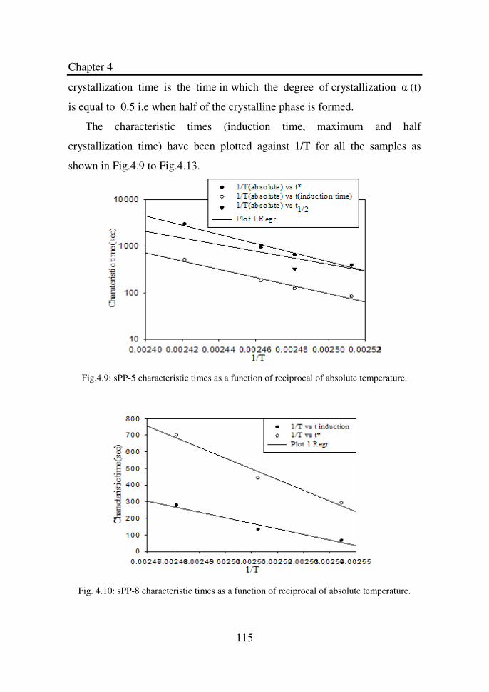
Chapter 4

115

crystallization time is the time in which the degree of crystallization α (t)

is equal to 0.5 i.e when half of the crystalline phase is formed.

The characteristic times (induction time, maximum and half

crystallization time) have been plotted against 1/T for all the samples as

shown in Fig.4.9 to Fig.4.13.

Fig.4.9: sPP-5 characteristic times as a function of reciprocal of absolute temperature.

Fig. 4.10: sPP-8 characteristic times as a function of reciprocal of absolute temperature.

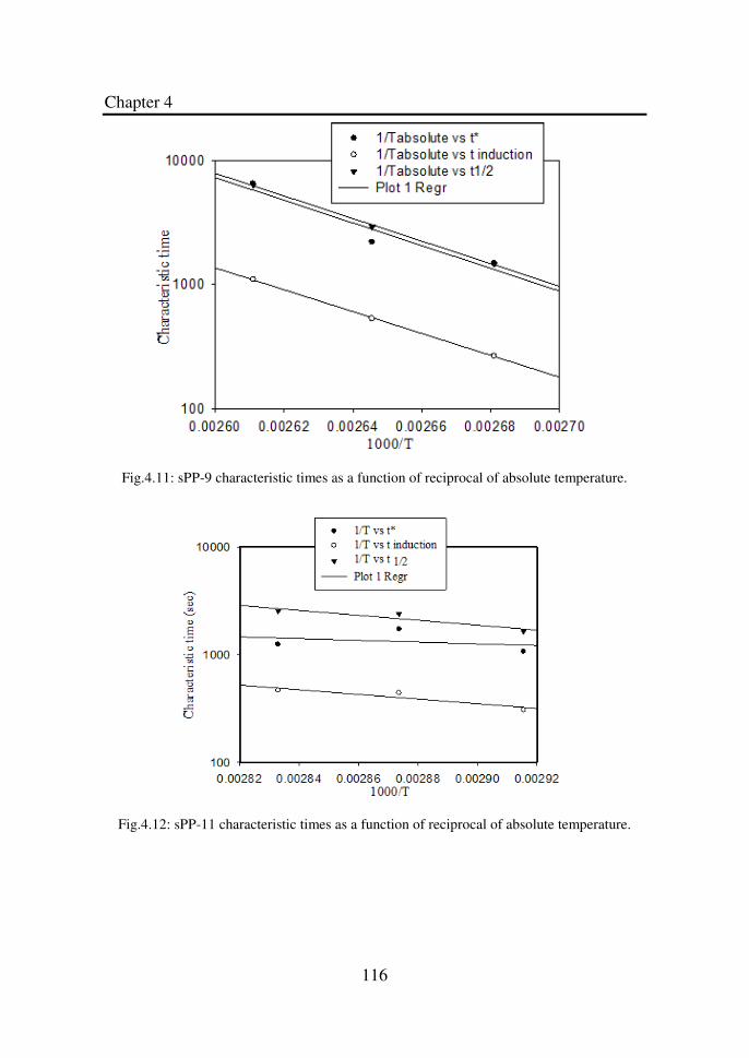
Chapter 4

116



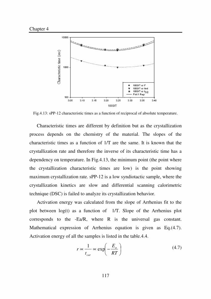
Chapter 4

117


Characteristic times are different by definition but as the crystallization

process depends on the chemistry of the material. The slopes of the

characteristic times as a function of 1/T are the same. It is known that the

crystallization rate and therefore the inverse of its characteristic time has a

dependency on temperature. In Fig.4.13, the minimum point (the point where

the crystallization characteristic times are low) is the point showing

maximum crystallization rate. sPP-12 is a low syndiotactic sample, where the

crystallization kinetics are slow and differential scanning calorimetric

technique (DSC) is failed to analyze its crystallization behavior.

Activation energy was calculated from the slope of Arrhenius fit to the

plot between log(t) as a function of 1/T. Slope of the Arrhenius plot

corresponds to the -Ea/R, where R is the universal gas constant.

Mathematical expression of Arrhenius equation is given as Eq.(4.7).

Activation energy of all the samples is listed in the table.4.4.

−∝∝

RT

E

tr a

car

exp1

(4.7)

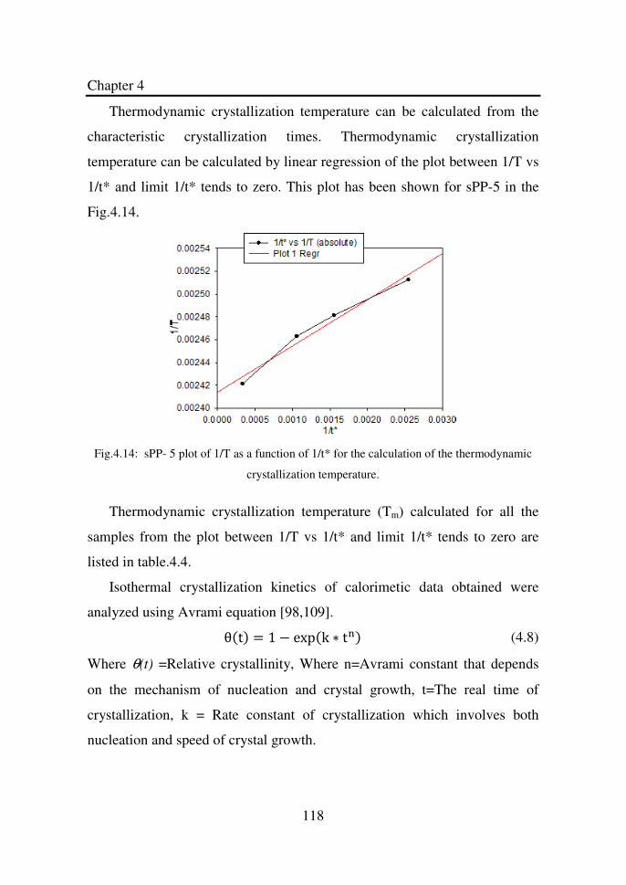
Chapter 4

118

Thermodynamic crystallization temperature can be calculated from the

characteristic crystallization times. Thermodynamic crystallization

temperature can be calculated by linear regression of the plot between 1/T vs

1/t* and limit 1/t* tends to zero. This plot has been shown for sPP-5 in the

Fig.4.14.

Fig.4.14: sPP- 5 plot of 1/T as a function of 1/t* for the calculation of the thermodynamic

crystallization temperature.

Thermodynamic crystallization temperature (Tm) calculated for all the

samples from the plot between 1/T vs 1/t* and limit 1/t* tends to zero are

listed in table.4.4.

Isothermal crystallization kinetics of calorimetic data obtained were

analyzed using Avrami equation [98,109].

θt = 1 − expk ∗ tD (4.8)

Where θ(t) =Relative crystallinity, Where n=Avrami constant that depends

on the mechanism of nucleation and crystal growth, t=The real time of

crystallization, k = Rate constant of crystallization which involves both

nucleation and speed of crystal growth.

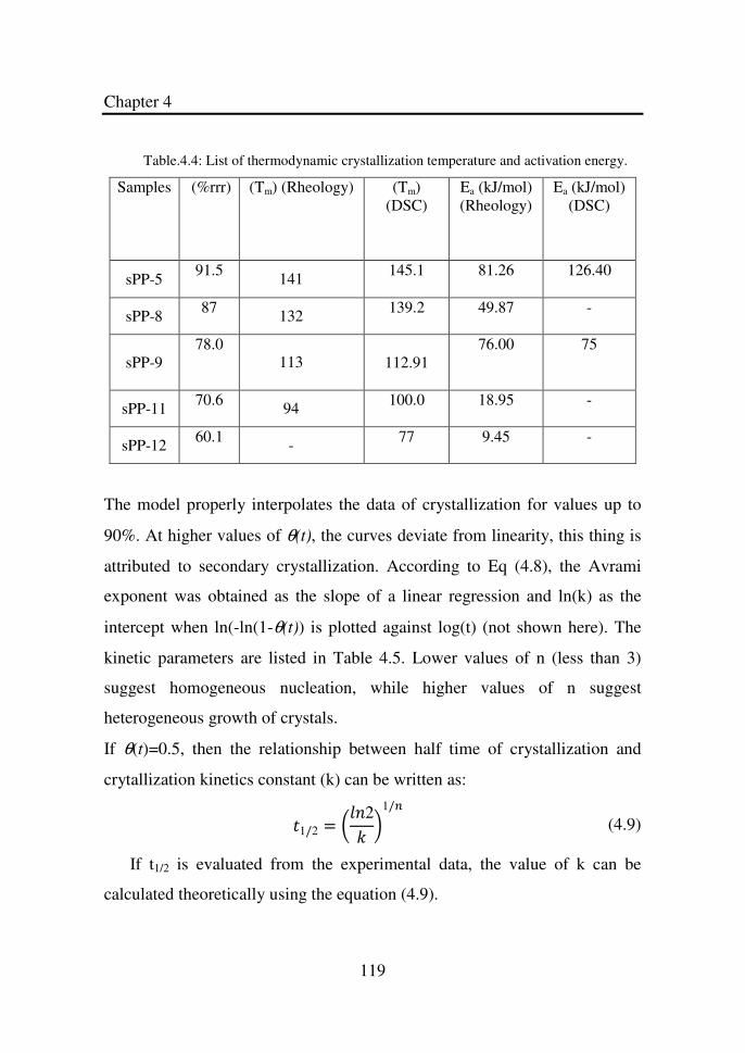
Chapter 4

119

Table.4.4: List of thermodynamic crystallization temperature and activation energy.

Samples (%rrr) (Tm) (Rheology) (Tm) (DSC)

Ea (kJ/mol) (Rheology)

Ea (kJ/mol) (DSC)

sPP-5 91.5 141 145.1

81.26 126.40

sPP-8 87 132 139.2 49.87 -

sPP-9 78.0

113

112.91

76.00 75

sPP-11 70.6 94 100.0 18.95 -

sPP-12 60.1 - 77 9.45 -

The model properly interpolates the data of crystallization for values up to

90%. At higher values of θ(t), the curves deviate from linearity, this thing is

attributed to secondary crystallization. According to Eq (4.8), the Avrami

exponent was obtained as the slope of a linear regression and ln(k) as the

intercept when ln(-ln(1-θ(t)) is plotted against log(t) (not shown here). The

kinetic parameters are listed in Table 4.5. Lower values of n (less than 3)

suggest homogeneous nucleation, while higher values of n suggest

heterogeneous growth of crystals.

If θ(t)=0.5, then the relationship between half time of crystallization and

crytallization kinetics constant (k) can be written as:

81/2 = )2

1/

(4.9)

If t1/2 is evaluated from the experimental data, the value of k can be

calculated theoretically using the equation (4.9).

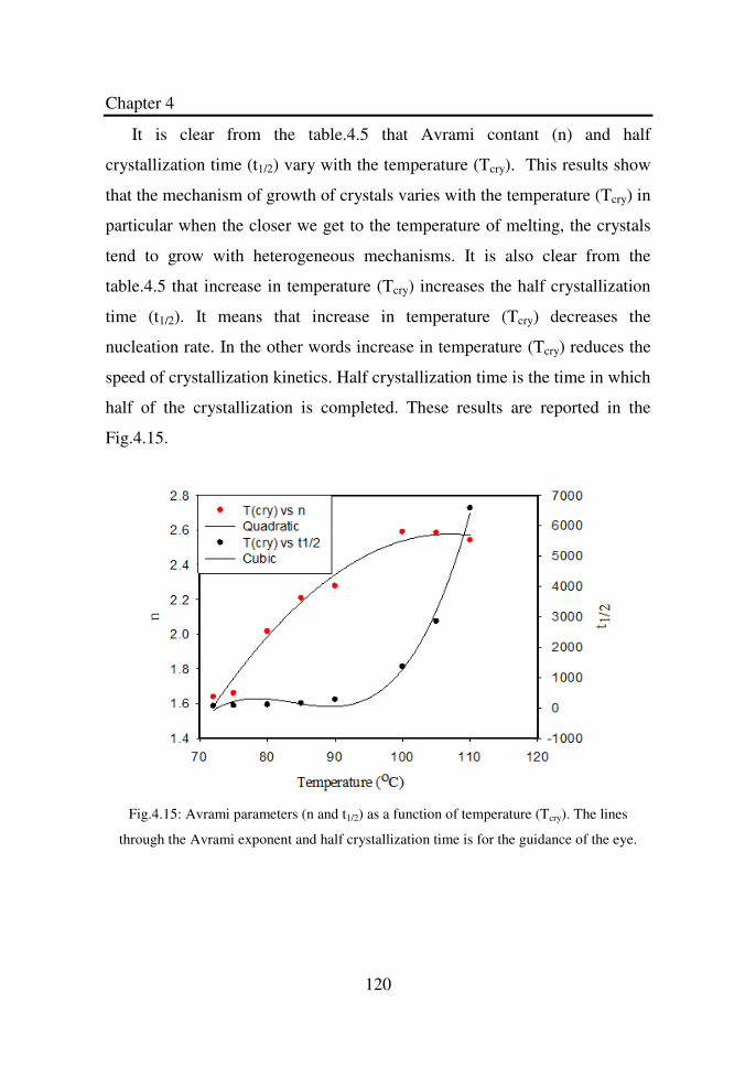
Chapter 4

120

It is clear from the table.4.5 that Avrami contant (n) and half

crystallization time (t1/2) vary with the temperature (Tcry). This results show

that the mechanism of growth of crystals varies with the temperature (Tcry) in

particular when the closer we get to the temperature of melting, the crystals

tend to grow with heterogeneous mechanisms. It is also clear from the

table.4.5 that increase in temperature (Tcry) increases the half crystallization

time (t1/2). It means that increase in temperature (Tcry) decreases the

nucleation rate. In the other words increase in temperature (Tcry) reduces the

speed of crystallization kinetics. Half crystallization time is the time in which

half of the crystallization is completed. These results are reported in the

Fig.4.15.

Fig.4.15: Avrami parameters (n and t1/2) as a function of temperature (Tcry). The lines

through the Avrami exponent and half crystallization time is for the guidance of the eye.

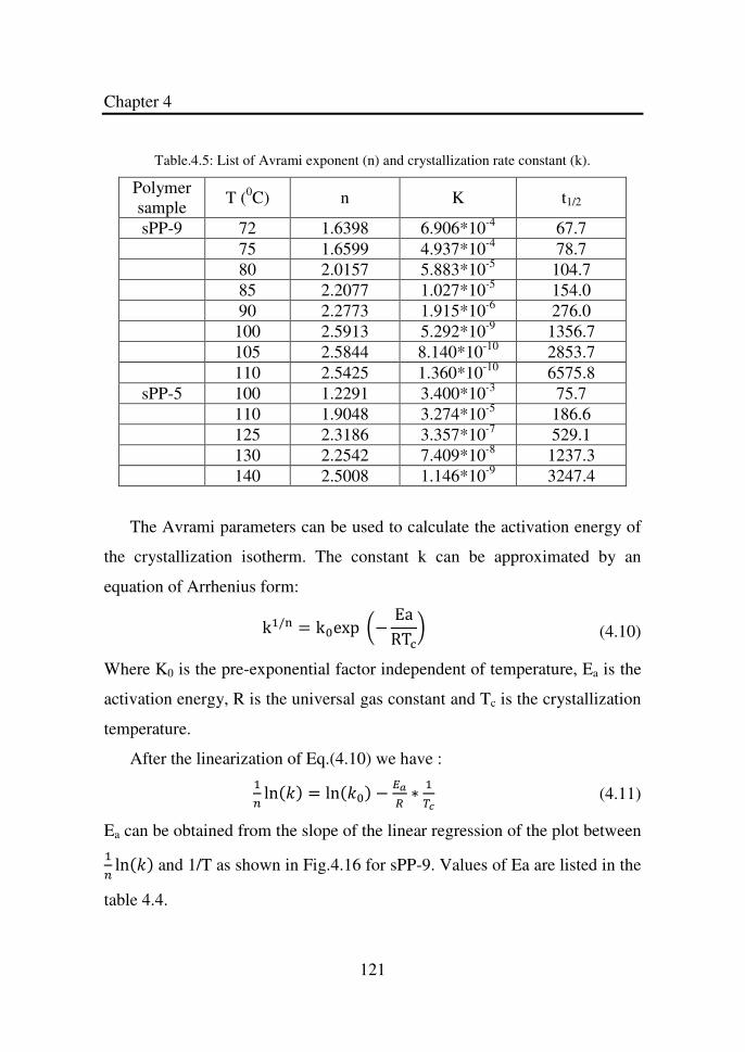
Chapter 4

121

Table.4.5: List of Avrami exponent (n) and crystallization rate constant (k).

Polymer sample

T (0C) n K t1/2

sPP-9 72 1.6398 6.906*10-4 67.7 75 1.6599 4.937*10-4 78.7 80 2.0157 5.883*10-5 104.7 85 2.2077 1.027*10-5 154.0 90 2.2773 1.915*10-6 276.0 100 2.5913 5.292*10-9 1356.7 105 2.5844 8.140*10-10 2853.7 110 2.5425 1.360*10-10 6575.8

sPP-5 100 1.2291 3.400*10-3 75.7 110 1.9048 3.274*10-5 186.6 125 2.3186 3.357*10-7 529.1 130 2.2542 7.409*10-8 1237.3 140 2.5008 1.146*10-9 3247.4

The Avrami parameters can be used to calculate the activation energy of

the crystallization isotherm. The constant k can be approximated by an

equation of Arrhenius form:

k/D = kexp − EaRTH

(4.10)

Where K0 is the pre-exponential factor independent of temperature, Ea is the

activation energy, R is the universal gas constant and Tc is the crystallization

temperature.

After the linearization of Eq.(4.10) we have : ln = ln − IJ

K ∗ LM

(4.11)

Ea can be obtained from the slope of the linear regression of the plot between ln and 1/T as shown in Fig.4.16 for sPP-9. Values of Ea are listed in the

table 4.4.

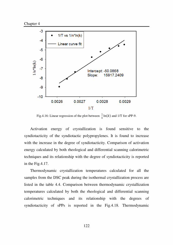
Chapter 4

122

Fig.4.16: Linear regression of the plot between ln and 1/T for sPP-9.

Activation energy of crystallization is found sensitive to the

syndiotacticity of the syndiotactic polypropylenes. It is found to increase

with the increase in the degree of syndiotacticity. Comparison of activation

energy calculated by both rheological and differential scanning calorimetric

techniques and its relationship with the degree of syndiotacticity is reported

in the Fig.4.17.

Thermodynamic crystallization temperatures calculated for all the

samples from the DSC peak during the isothermal crystallization process are

listed in the table 4.4. Comparison between thermodynamic crystallization

temperatures calculated by both the rheological and differential scanning

calorimetric techniques and its relationship with the degrees of

syndiotacticity of sPPs is reported in the Fig.4.18. Thermodynamic

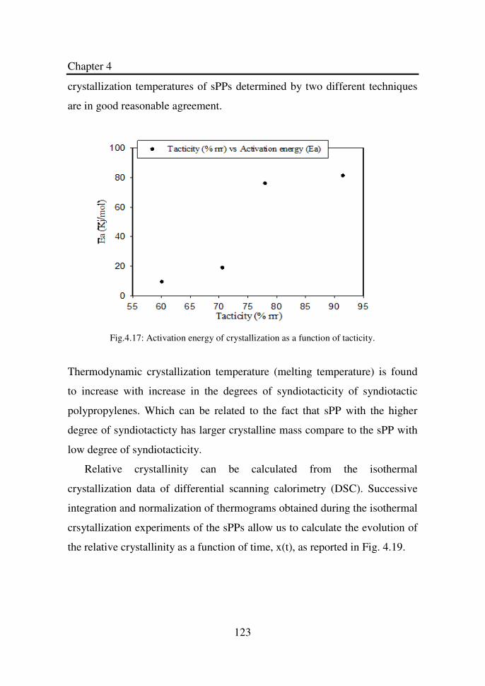
Chapter 4

123

crystallization temperatures of sPPs determined by two different techniques

are in good reasonable agreement.

Fig.4.17: Activation energy of crystallization as a function of tacticity.

Thermodynamic crystallization temperature (melting temperature) is found

to increase with increase in the degrees of syndiotacticity of syndiotactic

polypropylenes. Which can be related to the fact that sPP with the higher

degree of syndiotacticty has larger crystalline mass compare to the sPP with

low degree of syndiotacticity.

Relative crystallinity can be calculated from the isothermal

crystallization data of differential scanning calorimetry (DSC). Successive

integration and normalization of thermograms obtained during the isothermal

crsytallization experiments of the sPPs allow us to calculate the evolution of

the relative crystallinity as a function of time, x(t), as reported in Fig. 4.19.

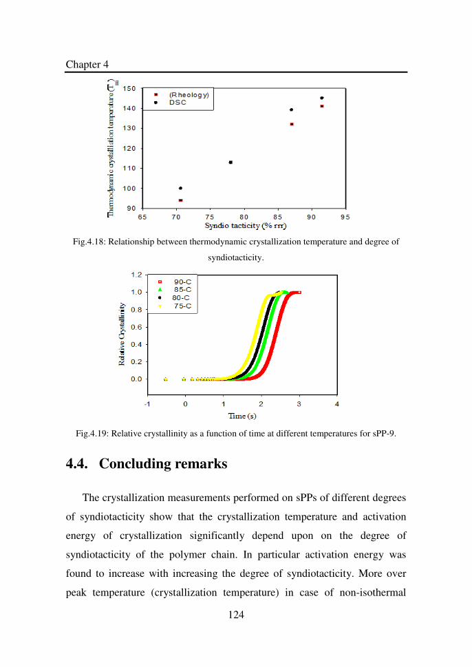
Chapter 4

124

Fig.4.18: Relationship between thermodynamic crystallization temperature and degree of

syndiotacticity.

Fig.4.19: Relative crystallinity as a function of time at different temperatures for sPP-9.

4.4. Concluding remarks

The crystallization measurements performed on sPPs of different degrees

of syndiotacticity show that the crystallization temperature and activation

energy of crystallization significantly depend upon on the degree of

syndiotacticity of the polymer chain. In particular activation energy was

found to increase with increasing the degree of syndiotacticity. More over

peak temperature (crystallization temperature) in case of non-isothermal

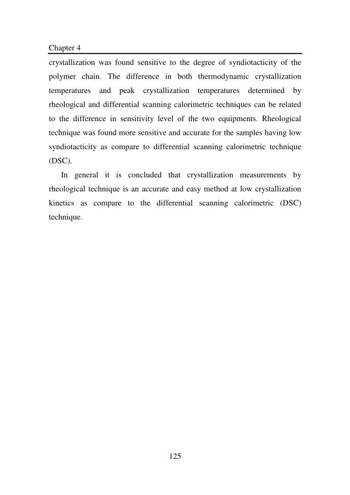
Chapter 4

125

crystallization was found sensitive to the degree of syndiotacticity of the

polymer chain. The difference in both thermodynamic crystallization

temperatures and peak crystallization temperatures determined by

rheological and differential scanning calorimetric techniques can be related

to the difference in sensitivity level of the two equipments. Rheological

technique was found more sensitive and accurate for the samples having low

syndiotacticity as compare to differential scanning calorimetric technique

(DSC).

In general it is concluded that crystallization measurements by

rheological technique is an accurate and easy method at low crystallization

kinetics as compare to the differential scanning calorimetric (DSC)

technique.

Chapter 5

126

Linear Viscoelasticity of Isotactic, Atactic and

Syndiotactic Poly-1Butenes

5.1. Introduction

The ability to predict the polymer properties like molecular weight,

polydispersity and molecular architecture from the knowledge of rheology is

one of the big achievements of polymer rheology. In Chapter 3 we have

already shown some relations between the viscoelastic response and the

molecular architecture of syndiotactic Polypropylene (sPP). Following the

same lines, in the present chapter we present a similar analysis for another

polyolefin, namely, Poly-1Butene. The importance of determining the

rheology of stereo-regular Poly-1Butenes is somewhat twofold. On the one

hand, unlike sPP, whose rheology has been the subject of different studies in

the literature, little or nothing is known about the linear viscoelastic response

of syndiotactic poly-1Butene. On the other hand, having a second, well

characterized syndiotactic polyolefin opens the way to a possible

confirmation of the role that stereo-regularity plays in determining the

rheological viscoelastic behavior in the melt state.

In order to achieve the above objectives, as it was the case in Chapter 3,

frequency sweep tests at different temperatures were conducted after

confirming the linearity by strain sweep tests. Master curves were obtained

by applying the Time Temperature Superposition principle using the

Orchestrator software. The plateau modulus was determined for all samples

by the best suitable method for the given shape of the viscoelastic curves.

Chapter 5

127

The entanglement molecular weight, as well as the packing length of the

different PB samples were calculated by using the correlation between

plateau modulus and entanglement molecular weight (reptation theory) [70],

and the models proposed by Fetters et al. [71].


5.2.1. Material

Three different samples of syndiotactic (sPB), atactic (aPB) and isotactic

(iPB) Poly-1Butene were used for the viscoelastic study. The relevant

properties of the polymers are reported in Table.5.1. The structure of the

poly-1Butene repeating unit is reported in Fig.5.1.

It can be noted from Table.5.1 that the syndio- and iso- samples are

characterized by high degree of tactitiy. Stereo-regularity data for the atactic

PB are not available. The sPB shows a very low value of the melting

temperature, which is also related to slow crystallization kinetics. Like

Polypropylene, iPB melts at a much higher temperature, and displays a much

faster kinetics.

Table 5.1: List of materials with some properties.

Sample Tm (°C) % (rrrr) % (mmmm) Mw sPB 39.2 96 115.000 aPB 339.000 iPB 134 99 430.000

Chapter 5

128

Fig. 5.1: Structure of the poly-1Butene repeating unit.

5.2.2. Methodology

All viscoelastic measurements were performed using the ARES rheometer

(TA Instruments) equipped with the 8 mm diameter parallel plate geometry

and commanded by the TA Orchestrator. Experiments were performed under

a nitrogen atmosphere (instead of air) in order to minimize thermal

degradation. All experiments were performed at a different gap depending on

the as provided sample thickness as provided. The gap thickness was always

in the order of 0.5 mm. Upon changes in temperature, the gap was always

adjusted to account for thermal expansion of the rheometer tool.

5.2.2.1.Dynamic strain sweep test

Dynamic strain sweep tests were performed at different temperatures and

a constant frequency of 10 rad/s for each sample in order to determine the

linearity limit. The strain was varied from 0.1 to 10 %.

Fig.5.2: Dynamic strain sweep test set-up screen.

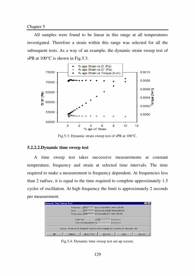
Chapter 5

129

All samples were found to be linear in this range at all temperatures

investigated. Therefore a strain within this range was selected for all the

subsequent tests. As a way of an example, the dynamic strain sweep test of

sPB at 100°C is shown in Fig.5.3.

Fig.5.3: Dynamic strain sweep test of sPB at 100°C.

5.2.2.2.Dynamic time sweep test

A time sweep test takes successive measurements at constant

temperature, frequency and strain at selected time intervals. The time

required to make a measurement is frequency dependent. At frequencies less

than 2 rad/sec, it is equal to the time required to complete approximately 1.5

cycles of oscillation. At high frequency the limit is approximately 2 seconds

per measurement.

Fig.5.4: Dynamic time sweep test set-up screen.

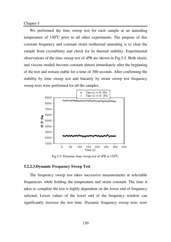
Chapter 5

130

We performed the time sweep test for each sample at an annealing

temperature of 1500C prior to all other experiments. The purpose of this

constant frequency and constant strain isothermal annealing is to clear the

sample from crystallinity and check for its thermal stability. Experimental

observations of the time sweep test of sPB are shown in Fig.5.5. Both elastic

and viscous moduli become constant almost immediately after the beginning

of the test and remain stable for a time of 300 seconds. After confirming the

stability by time sweep test and linearity by strain sweep test frequency

sweep tests were performed for all the samples.

Fig.5.5: Dynamic time sweep test of sPB at 1500C.

5.2.2.3.Dynamic Frequency Sweep Test

The frequency sweep test takes successive measurements at selectable

frequencies while holding the temperature and strain constant. The time it

takes to complete the test is highly dependent on the lower end of frequency

selected. Lower values of the lower end of the frequency window can

significantly increase the test time. Dynamic frequency sweep tests were

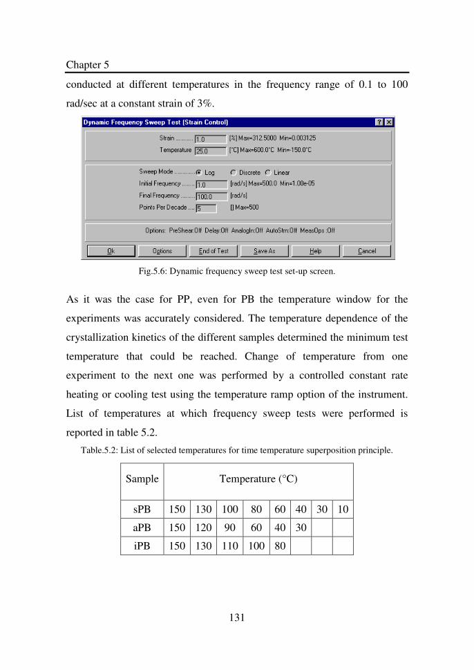
Chapter 5

131

conducted at different temperatures in the frequency range of 0.1 to 100

rad/sec at a constant strain of 3%.

Fig.5.6: Dynamic frequency sweep test set-up screen.

As it was the case for PP, even for PB the temperature window for the

experiments was accurately considered. The temperature dependence of the

crystallization kinetics of the different samples determined the minimum test

temperature that could be reached. Change of temperature from one

experiment to the next one was performed by a controlled constant rate

heating or cooling test using the temperature ramp option of the instrument.

List of temperatures at which frequency sweep tests were performed is

reported in table 5.2.

Table.5.2: List of selected temperatures for time temperature superposition principle.

Sample Temperature (°C)

sPB 150 130 100 80 60 40 30 10

aPB 150 120 90 60 40 30

iPB 150 130 110 100 80

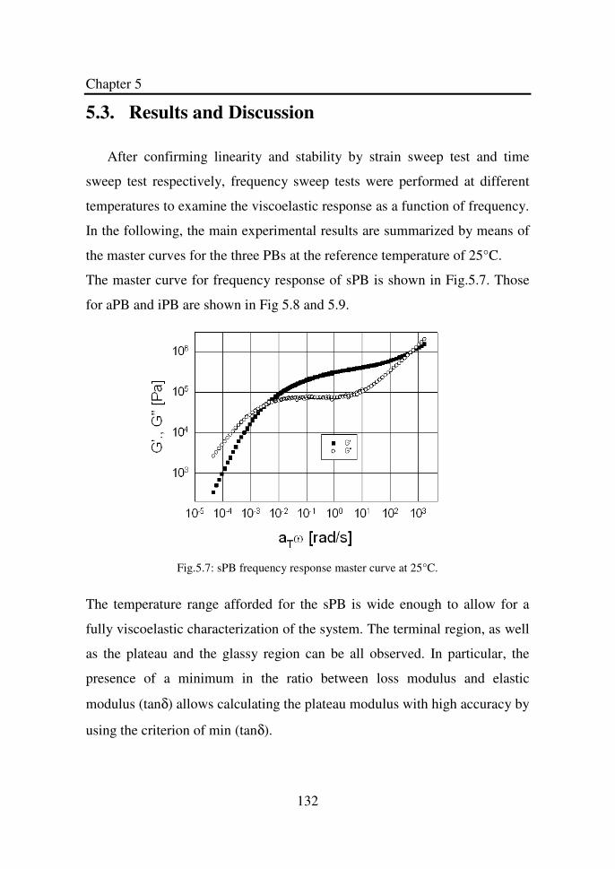
Chapter 5

132


After confirming linearity and stability by strain sweep test and time

sweep test respectively, frequency sweep tests were performed at different

temperatures to examine the viscoelastic response as a function of frequency.

In the following, the main experimental results are summarized by means of

the master curves for the three PBs at the reference temperature of 25°C.

The master curve for frequency response of sPB is shown in Fig.5.7. Those

for aPB and iPB are shown in Fig 5.8 and 5.9.

Fig.5.7: sPB frequency response master curve at 25°C.

The temperature range afforded for the sPB is wide enough to allow for a

fully viscoelastic characterization of the system. The terminal region, as well

as the plateau and the glassy region can be all observed. In particular, the

presence of a minimum in the ratio between loss modulus and elastic

modulus (tanδ) allows calculating the plateau modulus with high accuracy by

using the criterion of min (tanδ).

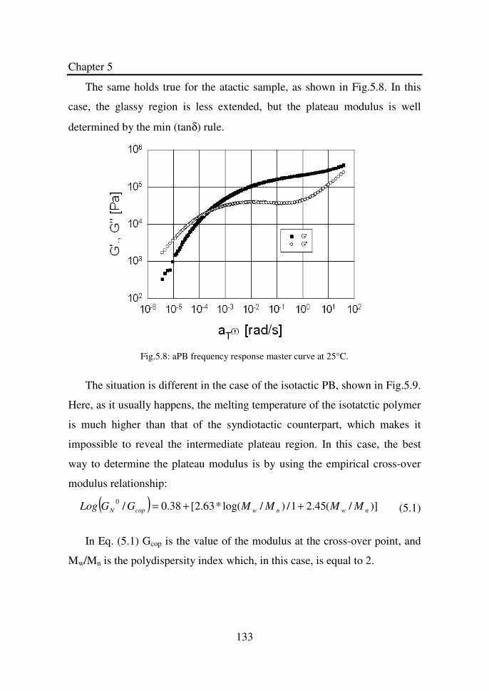
Chapter 5

133

The same holds true for the atactic sample, as shown in Fig.5.8. In this

case, the glassy region is less extended, but the plateau modulus is well

determined by the min (tanδ) rule.

Fig.5.8: aPB frequency response master curve at 25°C.

The situation is different in the case of the isotactic PB, shown in Fig.5.9.

Here, as it usually happens, the melting temperature of the isotatctic polymer

is much higher than that of the syndiotactic counterpart, which makes it

impossible to reveal the intermediate plateau region. In this case, the best

way to determine the plateau modulus is by using the empirical cross-over

modulus relationship:

( ) )]/(45.21/)/log(*63.2[38.0/0nwnwcopN MMMMGGLog ++=

(5.1)

In Eq. (5.1) Gcop is the value of the modulus at the cross-over point, and

Mw/Mn is the polydispersity index which, in this case, is equal to 2.

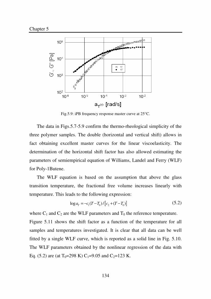
Chapter 5

134

Fig.5.9: iPB frequency response master curve at 25°C.

The data in Figs.5.7-5.9 confirm the thermo-rheological simplicity of the

three polymer samples. The double (horizontal and vertical shift) allows in

fact obtaining excellent master curves for the linear viscoelasticity. The

determination of the horizontal shift factor has also allowed estimating the

parameters of semiempirical equation of Williams, Landel and Ferry (WLF)

for Poly-1Butene. The WLF equation is based on the assumption that above the glass

transition temperature, the fractional free volume increases linearly with

temperature. This leads to the following expression:

[ ]1 0 2 0log ( ) / ( )T

a c T T c T T= − − + − (5.2)

where C1 and C2 are the WLF parameters and T0 the reference temperature.

Figure 5.11 shows the shift factor as a function of the temperature for all

samples and temperatures investigated. It is clear that all data can be well

fitted by a single WLF curve, which is reported as a solid line in Fig. 5.10.

The WLF parameters obtained by the nonlinear regression of the data with

Eq. (5.2) are (at T0=298 K) C1=9.05 and C2=123 K.

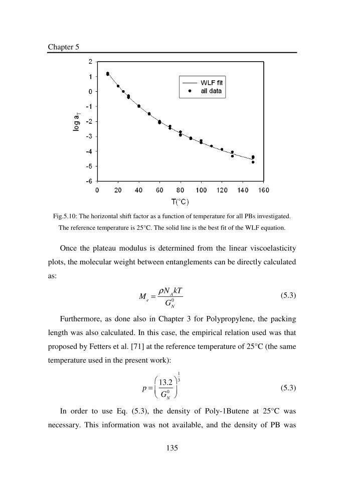
Chapter 5

135

Fig.5.10: The horizontal shift factor as a function of temperature for all PBs investigated.

The reference temperature is 25°C. The solid line is the best fit of the WLF equation.

Once the plateau modulus is determined from the linear viscoelasticity

plots, the molecular weight between entanglements can be directly calculated

as:

M

e=

ρNAkT

GN

0

(5.3)

Furthermore, as done also in Chapter 3 for Polypropylene, the packing

length was also calculated. In this case, the empirical relation used was that

proposed by Fetters et al. [71] at the reference temperature of 25°C (the same

temperature used in the present work):

p =13.2

GN

0

13

(5.3)

In order to use Eq. (5.3), the density of Poly-1Butene at 25°C was

necessary. This information was not available, and the density of PB was

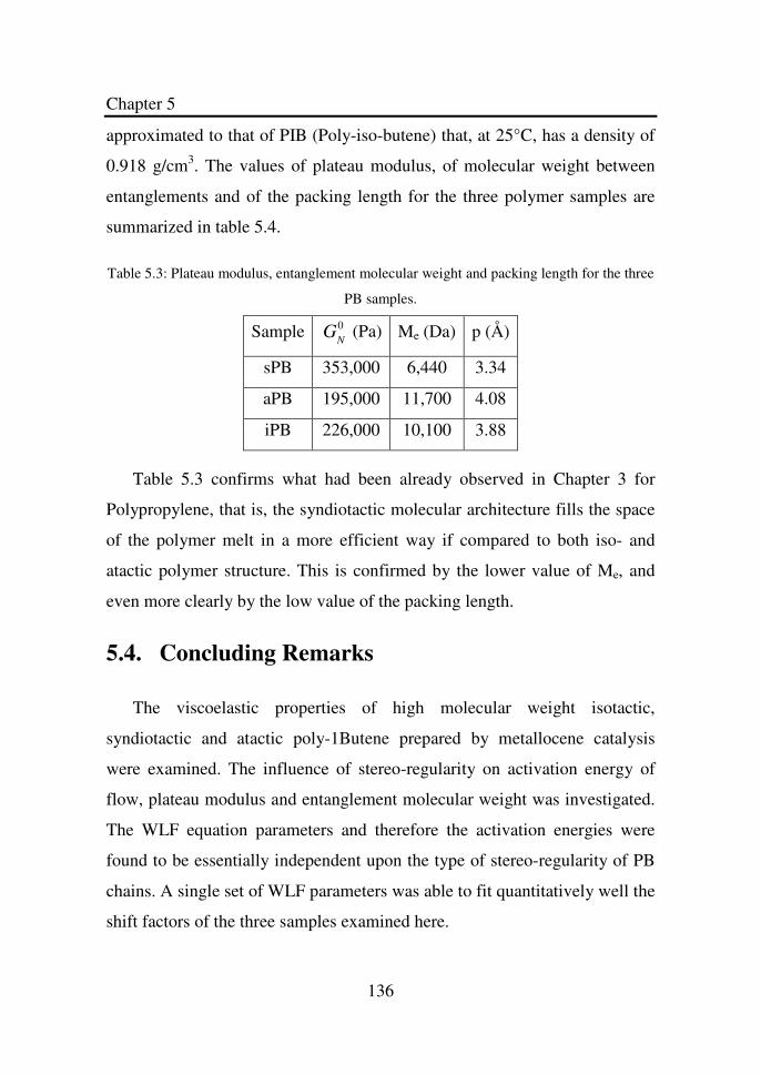
Chapter 5

136

approximated to that of PIB (Poly-iso-butene) that, at 25°C, has a density of

0.918 g/cm3. The values of plateau modulus, of molecular weight between

entanglements and of the packing length for the three polymer samples are

summarized in table 5.4.

Table 5.3: Plateau modulus, entanglement molecular weight and packing length for the three

PB samples.

Sample GN

0 (Pa) Me (Da) p (Å)

sPB 353,000 6,440 3.34

aPB 195,000 11,700 4.08

iPB 226,000 10,100 3.88

Table 5.3 confirms what had been already observed in Chapter 3 for

Polypropylene, that is, the syndiotactic molecular architecture fills the space

of the polymer melt in a more efficient way if compared to both iso- and

atactic polymer structure. This is confirmed by the lower value of Me, and

even more clearly by the low value of the packing length.

5.4. Concluding Remarks

The viscoelastic properties of high molecular weight isotactic,

syndiotactic and atactic poly-1Butene prepared by metallocene catalysis

were examined. The influence of stereo-regularity on activation energy of

flow, plateau modulus and entanglement molecular weight was investigated.

The WLF equation parameters and therefore the activation energies were

found to be essentially independent upon the type of stereo-regularity of PB

chains. A single set of WLF parameters was able to fit quantitatively well the

shift factors of the three samples examined here.

Chapter 5

137

Moving to the determination of the plateau modulus, both sPB and aPB

samples enabled the measurement of both elastic and viscous modulus over a

range necessary to obtain a significant onset of the plateau zone. The plateau

modulus of both the syndio and atactic PBs were determined successfully by

theoretically rigorous min (tanδ) method. In the case of isotactic PB the

plateau regime was not available and the plateau modulus was determined by

the empirical cross-over modulus method.

It was confirmed that the plateau modulus of syndio-PB was significantly

larger than that of the chemically equivalent but stereo-regularly different

aPB and iPB samples. This fact confirms what had been already observed in

chapter 3 for Polypropylene and gives more strength to the hypothesis that

the syndiotactic conformational arrangement is a more efficient space filling

architecture in the melt state.

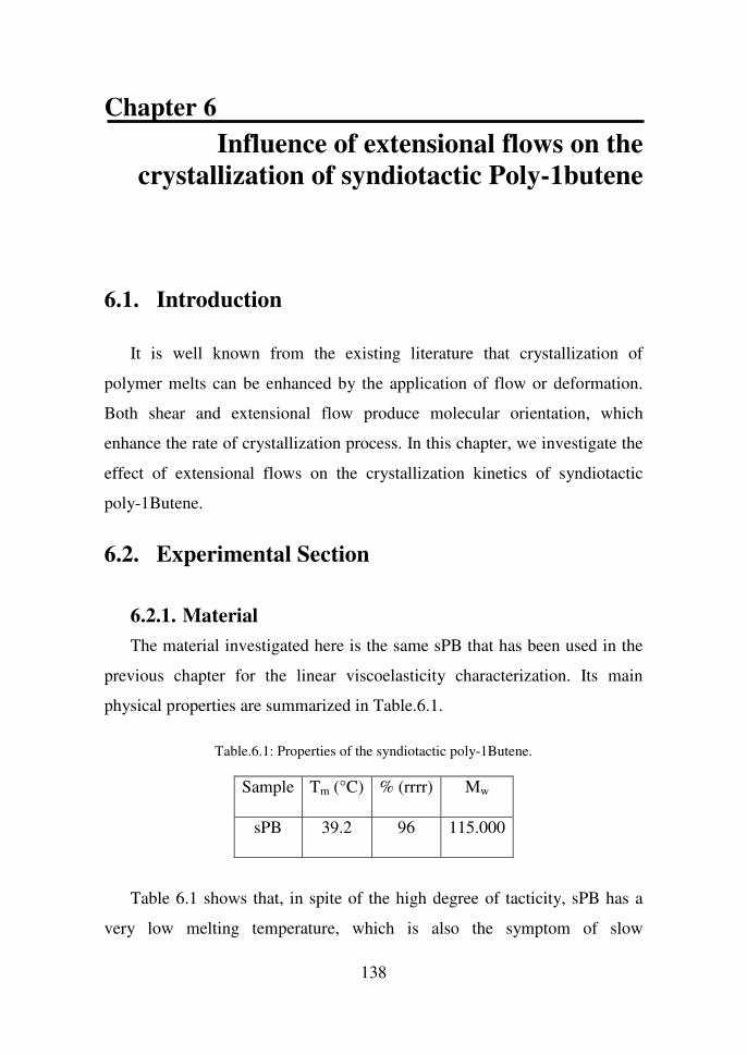
Chapter 6

138

Influence of extensional flows on the

crystallization of syndiotactic Poly-1butene

6.1. Introduction

It is well known from the existing literature that crystallization of

polymer melts can be enhanced by the application of flow or deformation.

Both shear and extensional flow produce molecular orientation, which

enhance the rate of crystallization process. In this chapter, we investigate the

effect of extensional flows on the crystallization kinetics of syndiotactic

poly-1Butene.


6.2.1. Material

The material investigated here is the same sPB that has been used in the

previous chapter for the linear viscoelasticity characterization. Its main

physical properties are summarized in Table.6.1.

Table.6.1: Properties of the syndiotactic poly-1Butene.

Sample Tm (°C) % (rrrr) Mw

sPB 39.2 96 115.000

Table 6.1 shows that, in spite of the high degree of tacticity, sPB has a

very low melting temperature, which is also the symptom of slow

Chapter 6

139

crystallization kinetics. For this reason, sPB is a good candidate to explore

the effect of flow and deformation on the crystallization process.

6.2.2. Methodology

All experiments shown in this chapter has been performed on samples

that received the same thermo-mechanical history. In particular, samples

were compression-molded in a Carver hydraulic press at the temperature of

70°C. This temperature is well above the melting point, thus guaranteeing

complete melting of the crystallites.

Quiescent crystallization was studied in two different ways. On the one

hand, calorimetric measurements were performed on a DSC apparatus

(Shimadzu, A60). On the other hand, small amplitude oscillatory time sweep

experiments were performed in the ARES rheometer at a frequency of 10

rad/s.

The stretch-induced crystallization experiments were performed by the

Sentmanat Extensional Rheometer (SER) attached to the ARES rheometer.

The Sentmanat Extensional Rheometer (SER) consists of two small cylinders

arranged in parallel. The sample is positioned between the cylinders at the

middle height using two clips. When attached to a rotational rheometer, such

as the, one cylinder is connected to the force transducer and the other to the

motor. The outer cylinder rotates around the inner one, while rotating on its

own axis. By this way the sample is stretched uniaxially. Different

extensional rates in the range of 0.001 to 7s-1 at a constant Hencky strain of 3

were applied at two different temperatures, namely, 40°C (slightly above the

melting temperature) and 25°C (well below the melting temperature). The

temperature is regulated by a forced convection chamber.

Stretch rheological experiments were also complemented by Small Angle

X-Ray Scattering (SAXS) experiments performed at the Department of

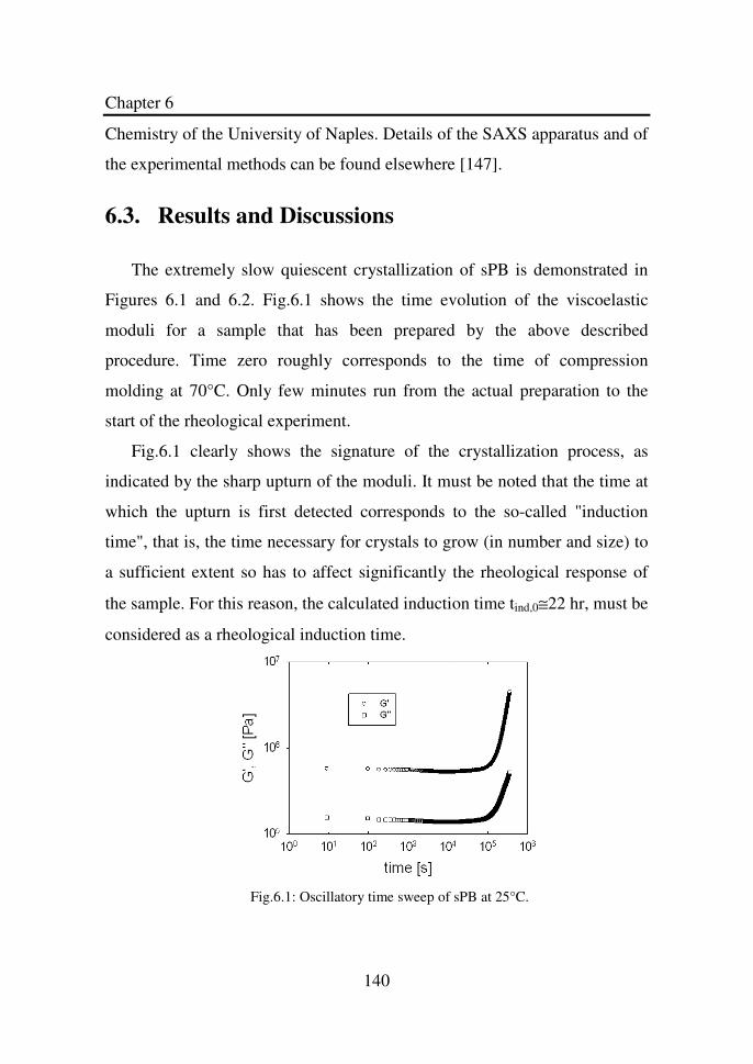
Chapter 6

140

Chemistry of the University of Naples. Details of the SAXS apparatus and of

the experimental methods can be found elsewhere [147].

6.3. Results and Discussions

The extremely slow quiescent crystallization of sPB is demonstrated in

Figures 6.1 and 6.2. Fig.6.1 shows the time evolution of the viscoelastic

moduli for a sample that has been prepared by the above described

procedure. Time zero roughly corresponds to the time of compression

molding at 70°C. Only few minutes run from the actual preparation to the

start of the rheological experiment.

Fig.6.1 clearly shows the signature of the crystallization process, as

indicated by the sharp upturn of the moduli. It must be noted that the time at

which the upturn is first detected corresponds to the so-called "induction

time", that is, the time necessary for crystals to grow (in number and size) to

a sufficient extent so has to affect significantly the rheological response of

the sample. For this reason, the calculated induction time tind,0≅22 hr, must be

considered as a rheological induction time.

Fig.6.1: Oscillatory time sweep of sPB at 25°C.

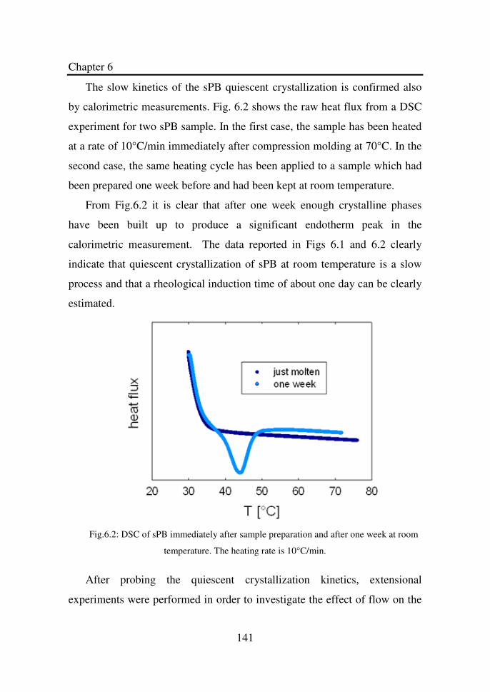
Chapter 6

141

The slow kinetics of the sPB quiescent crystallization is confirmed also

by calorimetric measurements. Fig. 6.2 shows the raw heat flux from a DSC

experiment for two sPB sample. In the first case, the sample has been heated

at a rate of 10°C/min immediately after compression molding at 70°C. In the

second case, the same heating cycle has been applied to a sample which had

been prepared one week before and had been kept at room temperature.

From Fig.6.2 it is clear that after one week enough crystalline phases

have been built up to produce a significant endotherm peak in the

calorimetric measurement. The data reported in Figs 6.1 and 6.2 clearly

indicate that quiescent crystallization of sPB at room temperature is a slow

process and that a rheological induction time of about one day can be clearly

estimated.

Fig.6.2: DSC of sPB immediately after sample preparation and after one week at room

temperature. The heating rate is 10°C/min.

After probing the quiescent crystallization kinetics, extensional

experiments were performed in order to investigate the effect of flow on the

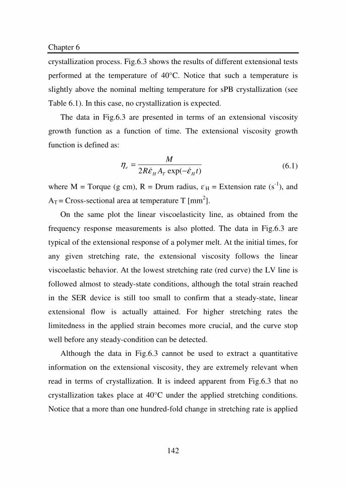
Chapter 6

142

crystallization process. Fig.6.3 shows the results of different extensional tests

performed at the temperature of 40°C. Notice that such a temperature is

slightly above the nominal melting temperature for sPB crystallization (see

Table 6.1). In this case, no crystallization is expected.

The data in Fig.6.3 are presented in terms of an extensional viscosity

growth function as a function of time. The extensional viscosity growth

function is defined as:

)exp(2 tAR

M

HTH

eεε

η&& −

=

(6.1)

where M = Torque (g cm), R = Drum radius, ɛ.H = Extension rate (s-1), and

AT = Cross-sectional area at temperature T [mm2].

On the same plot the linear viscoelasticity line, as obtained from the

frequency response measurements is also plotted. The data in Fig.6.3 are

typical of the extensional response of a polymer melt. At the initial times, for

any given stretching rate, the extensional viscosity follows the linear

viscoelastic behavior. At the lowest stretching rate (red curve) the LV line is

followed almost to steady-state conditions, although the total strain reached

in the SER device is still too small to confirm that a steady-state, linear

extensional flow is actually attained. For higher stretching rates the

limitedness in the applied strain becomes more crucial, and the curve stop

well before any steady-condition can be detected.

Although the data in Fig.6.3 cannot be used to extract a quantitative

information on the extensional viscosity, they are extremely relevant when

read in terms of crystallization. It is indeed apparent from Fig.6.3 that no

crystallization takes place at 40°C under the applied stretching conditions.

Notice that a more than one hundred-fold change in stretching rate is applied

Chapter 6

143

to sample without any apparent sign of qualitative change in its extensional

response.

Fig.6.3: Extensional viscosity growth function for sPB at 40°C. The linear viscoelasticity

line is also reported for reference.

The situation depicted in Fig.6.3 is drastically changed when the

extensional flow is applied at the temperature of 25°C. A summary of all

experiments conducted on sPB at this temperature is reported in Fig.6.4,

along with the LV line at the same temperature.

For the lowest stretching rate (10-3 s-1) the extensional responses closely

match the linear viscoelastic behavior, at least until sample breakup. Breakup

is in all cases indicated by the sudden down turn in the extensional curve.

Since the cross-over relaxation time of sPB at 25°C is about 270 s, the

corresponding Weissenberg number results to be We=0.27.

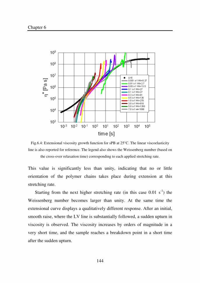
Chapter 6

144

Fig.6.4: Extensional viscosity growth function for sPB at 25°C. The linear viscoelasticity

line is also reported for reference. The legend also shows the Weissenberg number (based on

the cross-over relaxation time) corresponding to each applied stretching rate.

This value is significantly less than unity, indicating that no or little

orientation of the polymer chains takes place during extension at this

stretching rate.

Starting from the next higher stretching rate (in this case 0.01 s-1) the

Weissenberg number becomes larger than unity. At the same time the

extensional curve displays a qualitatively different response. After an initial,

smooth raise, where the LV line is substantially followed, a sudden upturn in

viscosity is observed. The viscosity increases by orders of magnitude in a

very short time, and the sample reaches a breakdown point in a short time

after the sudden upturn.

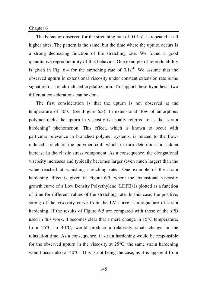
Chapter 6

145

The behavior observed for the stretching rate of 0.01 s-1 is repeated at all

higher rates. The pattern is the same, but the time where the upturn occurs is

a strong decreasing function of the stretching rate. We found a good

quantitative reproducibility of this behavior. One example of reproducibility

is given in Fig. 6.4 for the stretching rate of 0.1s-1. We assume that the

observed upturn in extensional viscosity under constant extension rate is the

signature of stretch-induced crystallization. To support these hypothesis two

different considerations can be done.

The first consideration is that the upturn is not observed at the

temperature of 40°C (see Figure 6.3). In extensional flow of amorphous

polymer melts the upturn in viscosity is usually referred to as the "strain

hardening" phenomenon. This effect, which is known to occur with

particular relevance in branched polymer systems, is related to the flow-

induced stretch of the polymer coil, which in turn determines a sudden

increase in the elastic stress component. As a consequence, the elongational

viscosity increases and typically becomes larger (even much larger) than the

value reached at vanishing stretching rates. One example of the strain

hardening effect is given in Figure 6.5, where the extensional viscosity

growth curve of a Low Density Polyethylene (LDPE) is plotted as a function

of time for different values of the stretching rate. In this case, the positive,

strong of the viscosity curve from the LV curve is a signature of strain

hardening. If the results of Figure 6.5 are compared with those of the sPB

used in this work, it becomes clear that a mere change in 15°C temperature,

from 25°C to 40°C, would produce a relatively small change in the

relaxation time. As a consequence, if strain hardening would be responsible

for the observed upturn in the viscosity at 25°C, the same strain hardening

would occur also at 40°C. This is not being the case, as it is apparent from

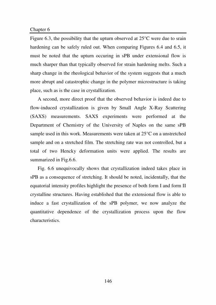
Chapter 6

146

Figure 6.3, the possibility that the upturn observed at 25°C were due to srain

hardening can be safely ruled out. When comparing Figures 6.4 and 6.5, it

must be noted that the upturn occuring in sPB under extensional flow is

much sharper than that typically observed for strain hardening melts. Such a

sharp change in the rheological behavior of the system suggests that a much

more abrupt and catastrophic change in the polymer microstructure is taking

place, such as is the case in crystallization.

A second, more direct proof that the observed behavior is indeed due to

flow-induced crystallization is given by Small Angle X-Ray Scattering

(SAXS) measurements. SAXS experiments were performed at the

Department of Chemistry of the University of Naples on the same sPB

sample used in this work. Measurements were taken at 25°C on a unstretched

sample and on a stretched film. The stretching rate was not controlled, but a

total of two Hencky deformation units were applied. The results are

summarized in Fig.6.6.

Fig. 6.6 unequivocally shows that crystallization indeed takes place in

sPB as a consequence of stretching. It should be noted, incidentally, that the

equatorial intensity profiles highlight the presence of both form I and form II

crystalline structures. Having established that the extensional flow is able to

induce a fast crystallization of the sPB polymer, we now analyze the

quantitative dependence of the crystallization process upon the flow

characteristics.

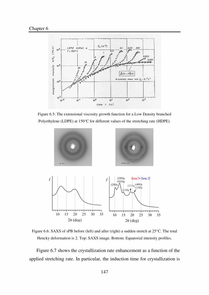
Chapter 6

147

Figure 6.5: The extensional viscosity growth function for a Low Density branched

Polyethylene (LDPE) at 150°C for different values of the stretching rate (HDPE).

Figure 6.6: SAXS of sPB before (left) and after (right) a sudden stretch at 25°C. The total

Hencky deformation is 2. Top: SAXS image. Bottom: Equatorial intensity profiles.

Figure 6.7 shows the crystallization rate enhancement as a function of the

applied stretching rate. In particular, the induction time for crystallization is

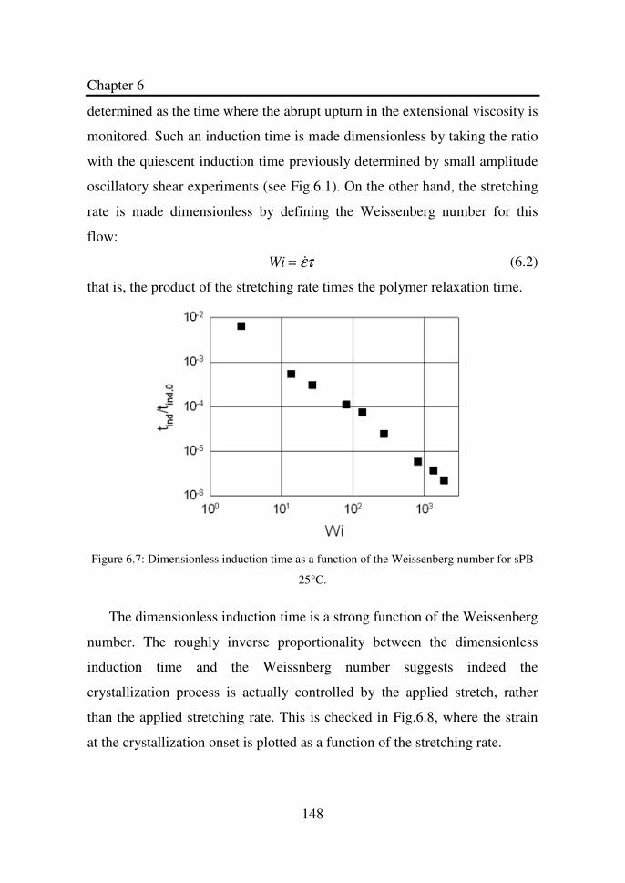
Chapter 6

148

determined as the time where the abrupt upturn in the extensional viscosity is

monitored. Such an induction time is made dimensionless by taking the ratio

with the quiescent induction time previously determined by small amplitude

oscillatory shear experiments (see Fig.6.1). On the other hand, the stretching

rate is made dimensionless by defining the Weissenberg number for this

flow:

Wi = &ετ (6.2)

that is, the product of the stretching rate times the polymer relaxation time.

Figure 6.7: Dimensionless induction time as a function of the Weissenberg number for sPB

25°C.

The dimensionless induction time is a strong function of the Weissenberg

number. The roughly inverse proportionality between the dimensionless

induction time and the Weissnberg number suggests indeed the

crystallization process is actually controlled by the applied stretch, rather

than the applied stretching rate. This is checked in Fig.6.8, where the strain

at the crystallization onset is plotted as a function of the stretching rate.

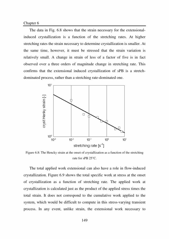
Chapter 6

149

The data in Fig. 6.8 shows that the strain necessary for the extensional-

induced crystallization is a function of the stretching rates. At higher

stretching rates the strain necessary to determine crystallization is smaller. At

the same time, however, it must be stressed that the strain variation is

relatively small. A change in strain of less of a factor of five is in fact

observed over a three orders of magnitude change in stretching rate. This

confirms that the extensional induced crystallization of sPB is a stretch-

dominated process, rather than a stretching rate-dominated one.

Figure 6.8: The Hencky strain at the onset of crystallization as a function of the stretching

rate for sPB 25°C.

The total applied work extensional can also have a role in flow-induced

crystallization. Figure 6.9 shows the total specific work at stress at the onset

of crystallization as a function of stretching rate. The applied work at

crystallization is calculated just as the product of the applied stress times the

total strain. It does not correspond to the cumulative work applied to the

system, which would be difficult to compute in this stress-varying transient

process. In any event, unlike strain, the extensional work necessary to

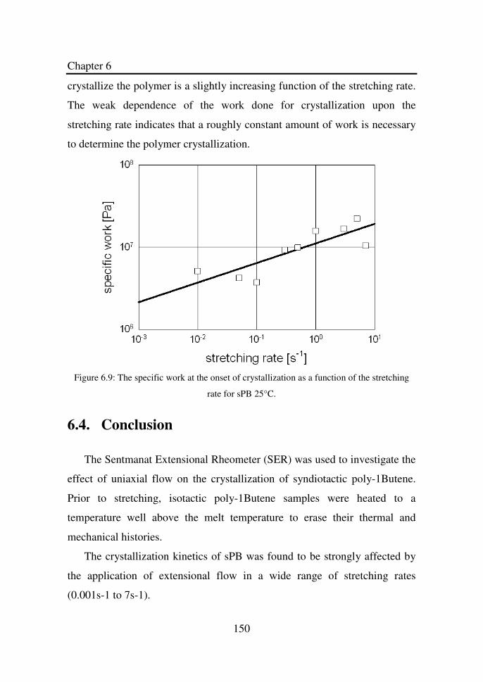
Chapter 6

150

crystallize the polymer is a slightly increasing function of the stretching rate.

The weak dependence of the work done for crystallization upon the

stretching rate indicates that a roughly constant amount of work is necessary

to determine the polymer crystallization.

Figure 6.9: The specific work at the onset of crystallization as a function of the stretching

rate for sPB 25°C.

6.4. Conclusion

The Sentmanat Extensional Rheometer (SER) was used to investigate the

effect of uniaxial flow on the crystallization of syndiotactic poly-1Butene.

Prior to stretching, isotactic poly-1Butene samples were heated to a

temperature well above the melt temperature to erase their thermal and

mechanical histories.

The crystallization kinetics of sPB was found to be strongly affected by

the application of extensional flow in a wide range of stretching rates

(0.001s-1 to 7s-1).

Chapter 6

151

The experimental data seem to suggest that the extension enhanced

crystallization process is controlled more by the applied deformation

(stretch) than by the deformation rate (stretching rate).

Chapter 7

152

Conclusion

In the present research work relationships between rheological

parameters and molecular structure of syndiotactic polypropylenes (sPP) and

poly-1Butenes of different stereoregularity are explored by performing

oscillatory shear experiments using ARES rheometer. Crystallization

behavior of a series of syndiotactic polypropylenes of different degrees of

syndiotacticity is investigated by performing both isothermal and non-

isothermal crystallization tests using rheological and differential scanning

calorimetric (DSC) techniques. The aim is to clarify the effect of degree of

syndiotacticity on the crystallization behavior of the syndiotactic

polypropylene. The effect of extensional flow on the crystallization kinetics

of sPB is examined both in the melt and crystal phase by applying different

extensional rates using sentmanat extensional rheometer (SER).

Rheological parameters, plateau modulus and entanglement molecular

weight are found very sensitive to the degree of syndiotacticity of

syndiotactic polypropylene (sPP). Plateau modulus is found to increase with

increase in the degree of syndiotacticity and consequently entanglement

molecular weight is found to decrease with increase in the degree of

syndiotacticiy of syndiotactic polypropylene (sPP). The same situation was

found for PBs. Rheological parameters, plateau modulus and therefore

entanglement molecular weight are found dependent on stereoregularity. It is

concluded that the sensitivity of rheological parameters to stereoregularity is

true for both the sPP and PBs.

Chapter 7

153

Crystallization behavior is found very sensitive to the degree of

syndiotacticity of sPP. Both activation energy and peak temperature

determined by non-isothermal crystallization are found to increase with

increase in the degree of syndiotacticity. Thermodynamic crystallization

temperature determined by isothermal crystallization is also found to

increase with increase in the degree of syndiotacticity of sPP. The difference

in the crystallization measurements made by the rheological and differential

scanning calorimetric techniques can be related to the difference in

sensitivity to temperature of the two equipments. Rheological technique is

found more sensitive and accurate for the samples having low syndiotacticity

as compare to differential scanning calorimetric technique (DSC). Because at

low syndiotacticity, the samples have small crystalline material and

consequently have low crystallization kinetics. In general it is concluded that

crystallization measurements by rheological technique is an accurate and

easy method at low crystallization kinetics as compare to the differential

scanning calorimetric (DSC) technique.

The crystallization process is investigated under the action of extensional

flow by using sentmant extensional rheometer (SER). The crystallization

kinetics of syndiotactic poly-1Butene is found very strongly affected by the

application of extensional flow in the crystal form. Nucleation rate and

therefore crystallization kinetics are found to increase with increase in the

extensional rate.

The present research work can be further extended by studying the effect

of syndiotacticity on rheological and crystallization behavior of the

crystalline elastomer co-polymers. The effect of extensional flow on the

crystallization behavior of poly-1Butenes and polypropylenes of different

stereoregularity can be explored and influence of stereoregularity on the

Chapter 7

154

crystallization process can be investigated. The results of this research work

are expected to be useful for the assessment of alternatives, actual synthesis

and applications of poly-olefins in polymer and processing industries.

155

References

[1] A.B.Samsuri, "Degradation of natural rubber and synthetic

elastomers", in "Shreir's Corrosion", Elsevier (2010) pp.2407-2438.

[2] H.Barnes, J.F.Hutton, K.Walters, "An introduction to rheology",

Elsevier 1989.

[3] W. McKeen, "The effect of temperature and other factors on plastics

and elastomers", 2nd edition, William Andrew Inc. 2008.

[4] J.Li, H.Li, C.Wu, Y.Ke, D.Wang, Q.Li, L.Zhang, Y.Hu.,

"Morphologies, crystallinity and dynamic mechanical

characterizations of polypropylene/polystyrene blends compatibilized

with PP-g-PS copolymer: Effect of the side chain length", Eur.

Polym. J. (2009), 45 2619-2628.

[5] K.W. JR., “Crystallinity of cellulose and its significance for the fiber

properties”, Txt. Res. J. (1950), 20, 363-372.

[6] W.Kaminsky., “New polyolefins by metallocene catalysts”, Pure &

Appl. Chem. (1998), 70, 1229-1233.

[7] F.Auriemma, O.R.Ballwesteros, C.D.Rosa., “Origin of the elastic

behavior of syndiotactic polypropylene”, Macromolecules. ( 2001),

34, 4485-4491.

[8] F.Auriemma, C.De Rosa., “New concepts in thermoplastic

elastomers: the case of syndiotactic polypropylene, an

unconventional elastomer with high crystallinity and large modulus”,

J. Am. Chem.Soc. (2003), 125, 13143-7.

REFERENCES

156

[9] V.De La Torre, J.A.Rodriguez Fris, M.D.Failla, L.M.Quinzani.,

“Effect of melt annealing on the phase structure and rheological

behavior of propylene-ethylene copolymers”,Poly.Eng.Sci. (2007),

47, 912-921.

[10] J.Wang, Z.Yea, H.Fan, B.G.Li, S.Zhu., “Dynamic mechanical and

rheological properties of metallocene-catalyzed long-chain-branched

ethylene/propylene copolymers”, Polymer. (2004), 45, 5497-5504.

[11] A.Eckstein,C.Friedrich, A.Lobbrecht, R.Spitz, R.Mulhaup.,

“Comparison of the viscoelastic Properties of Syndiotactic and

Isotactic Polypropylenes”, Acta Polym. (1997), 48,41-46.

[12] S.Acierno, R.Pasquino, N.Grizzuti., “Rheological techniques for the

determination of the crystallization kinetics of a polypropylene–EPR

copolymer”, J.Therm.Anal.Calorim. (2009), 98, 639-644.

[13] J.M.Dealy,R.G.Larson,“Structure and rheology of molten polymers”,

Hanser publisher, 2006.

[14] R.J. Young, P.A.Lovell, “Introduction to polymers”, Chapman &

Hall, 1987.

[15] O.G.Lewi,R.M.J.R.King,“Free radical polymerization kinetics of

immobilized chains bulk polymerization of acrylonitrile”,“Advances

in chemistry” ACS (1969)pp. 25-45.

[16] D.J.Metz.“Radiation-induced ionic Anionic free radical polymers of

α-olefins polymerization”,“Advances in chemistry”,ACS(1969)

pp.202 -218.

[17] M.Szwarc, “Mechanism of propagation of ionic polymerizations”,

“Advances in chemistry”,ACS(1969) pp.236-249.

[18] J.Jezl, N.S.Chu, I.H.M.Khelghatian, “Anionic Free radical polymers

of α-olefins”, “Advances in chemistry”,ACS(1969) pp.268-286.

REFERENCES

157

[19] V.Jaacks,“Cationic copolymerization of trioxane and 1,3-

dioxolane”,“Advances in chemistry”,ACS(1969)pp.371-386.

[20] P.Cossee., “Ziegler-Natta catalysis I. Mechanism of polymerization

of α-olefins with Ziegler-Natta catalysts”, J.Catal. (1964), 3, 80-88.

[21] V.A.Kormer,B.D.Babitskiy and M.I.Lobach,“Stereospecific polymer-

-ization of 1,3-butadiene initiated by the transition metal π-

complexes”, “Advances in chemistry”, ACS(1969)pp.306-316.

[22] P.Cossee.,“On the reaction mechanism of the ethylene

polymerization with heterogeneous ziegler-natta catalysts”,

Tetrahedron Lett. (1960), 38,12-16.

[23] A.Zambelli, C.Tosi.,“Stereochemistry of propylene polymerization”,

Adv.Polym.Sci. (1974), 15, 31-60.

[24] G.Natta,I.Pasquon,A.Zambelli.,“Stereospecific catalysts for the

head-to-tail polymerization of propylene to a crystalline syndiotacfic

polymer”, J.Am.Chem.Soc. (1962), 84,1488-90.

[25] A. Zambelli, G.Natta, I.Pasquon.,“Polymerization of propylene to a

syndiotactic polymer”, J Polym Sci. (1963), 4, 411-26.

[26] Y.Doi, S.Suzuki , K.Soga.,“A perfect initiator for living co-

ordination polymerization of propene: tris(2-methyl-1,3

butanedionato) vanadium/diethylaluminium chloride system”,

Makromol. Chem. Rapid. Commun. (1985), 6,639-42.

[27] A.Zambelli, G.Natta, I.Pasquon, R.Signorini.,“Polymerization of

propylene to syndiotactic polymer. II. Behavior of the catalytic

system vanadium(IV) chloride-chorodiethylaluminum”, J Polym. Sci.

Polym.Symp. (1967), C16, 2485-99.

[28] A.Zambelli, I.Pasquon, R.Signorini, G.Natta.,“Polymerization of

propylene to syndiotactic polymer. III. Behavior of the catalyst

REFERENCES

158

system vanadium tetrachloride-diethylaluminum chloride in the

presence of Lewis bases”, Makromol Chem. (1968), 112, 160-82.

[29] G.Natta, A.Zambelli, G.Lanzi, I.Pasquon, E.R.Mognaschi,

A.L.Segre., “Polymerization of propylene to syndiotactic polymer

part1: Valence of active vanadium in the catalytic systems”,

Makromol.Chem. (1965), 81,161-72.

[30] M.Y.D.Reardon,S.Gambarotta,Y.G.Zahalka,H.L.C.Hyder.,“Vanadiu

m-catalyzed ethylene -propylene copolymerization: the question of

the metal oxidation state in zieglernatta polymerization promoted by

(b-diketonate)3V”, Organomet. Chem. (1999), 18, 2773-81.

[31] D.Y.M.Takada, T.Keii.,“Stereochemical structure and molecular

weight distribution of polypropylenes prepared with vanadium-based

catalyst systems”, Makromol.Chem.(1979), 180, 57-64.

[32] A. Zambelli, M.G.Giongo, G.Natta.,“Polymerization of propylene to

syndiotactic polymer. IV. Addition to the double bond”,

Makromol.Chem. (1968), 112,183-96.

[33] P.Locatelli, M.C.Sacchi, E.Rigamonti, A.Zambelli.,“Syndiotactic

polymerization of propene: regiospecificity of the initiation step”,

Macromolecules. (1984), 17,123-5.

[34] A.Zambelli, C.Tosi, C.Sacchi., “Polymerization of propylene to

syndiotactic polymer. VI. Monomer insertion”, Macromolecules.

(1972), 5, 649-54.

[35] A.Zambelli, C.Wolfsgruber, G.Zannoni, FA.Bovey., “Polymerization

of propylene to syndiotactic polymer. VIII. Steric control forces”,

Macromolecules. (1974), 7, 750-2.

REFERENCES

159

[36] A.Zambelli, P.Ammendola., “Stereospecific polymerization of a-

olefins: end groups, polymer structure and reaction mechanism”,

Prog.Polym.Sci. (1991), 16,203-18.

[37] A.Zambelli, I.Sessa, F.Grisi , R.Fusco, P.Accomazzi., “Syndiotactic

polymerization of propylene: single-site vanadium catalysts in

comparison with zirconium and nickel”, Macromol.Rapid.Commun.,

22 (2001) 297-310.

[38] Y.Doi, T.Koyama, K.Soga, T.Asakura., “Stereochemistry in living

co-ordination polymerization of propene initiated by vanadium-based

catalytic systems”, Makromol. Chem. (1984), 185,1827-33.

[39] Y.Doi, S.Ueki, T.Keii., “Living coordination polymerization of

propene initiated by the soluble V(acac)3-Al(C2H5)2Cl system”,

Macromolecules. (1979), 12, 814-819.

[40] Y.Doi, S.Ueki, T.Keii., “Preparation of living polypropylenes by a

soluble vanadium-based Ziegler catalyst”, Makromol. Chem.

(1979),180, 1359-61.

[41] J.A.Ewen., “Mechanism of stereochemical control in propylene

polymerizations with soluble group 4B metallocene/methylalumoxane

catalysts”,J.Am.Chem.Soc.(1984),106 ,6355-6364.

[42] W.Kaminsky,K.Kulper,H.H.Brintzinger,F.R.W.Wild.,“Polymerizati-

-on of propene and butene with a chiral zirconocene and

methylaluminoxane as co-catalyst”, Angew.Chem. (1985), 97, 507-

508.

[43] H.Sinn, W.Kaminsky, W.J.Vollmer, R.Woldt., “Living polymers with

Ziegler catalysts of high productivity”, Angew.Chem. Int.Ed.Engl.

(1980), 92,396-402.

REFERENCES

160

[44] J.A.Ewen, R.L.Jones, A.Razavi, J.D.Ferrara.,“Syndiospecific

propylene polymerizations with GroupIVB metallocenes”,

J.Am.Chem.Soc. (1988), 110, 6255-6256.

[45] A.Razavi, J.L.Atwood.,“Synthesis and characterization of the

catalytic isotactic-specific metallocene complex (h5-C5H3C4H9-CMe2-

h5-C13H8)ZrCl2:Mechanistic aspects of the formation of isotactic

polypropylene, the stereoregulative effect of the distal substituent and

the relevance of C2 symmetry”, J.Organomet.Chem. (1996), 520,115-

20.

[46] K.Mislow, M.Raban.,“Stereoisomeric relations of groups in

molecules”,Top Stereochem. (1967), 1,1-38. [47] LA.Castonguay, A.K.Rappe, Z.Natta., “A theoretical study of the

isotactic polymeri -zation of propylene”, J.Am.Chem.Soc. (1992),

114, 5832-42. [48] Z.Yu, J.C.W.Chien.,“ansa-Zirconocenium catalysis of syndiospecific

polymerization of propylene: theory and experiment”, J.Polym.Sci.

Part A Polym.Chem. (1995), 33,1085-1094. [49] JA.Ewen, M.J.Elder, R.L.Jones, L.Haspelagh, J.L.Atwood, S.G.Bott.,

“Metallocene/ polypropylene structural relationships:implications on

polymerization and stereochemical control mechanisms”,

Macromol.Symp. (1991), 1,253-295. [50] G.Balbontin, D.Dainelli, M.Galimberti, G.Paganetto.,“Thermal

behaviour of highly stereoregular syndiotactic polypropene from

homogeneous catalysts”, Macromol.Chem. (1992), 193, 693-703. [51] J.A.Ewen, L.Haspeslagh, J.L.Atwood, H. Zhang., “Crystal structures

and stereospecific propylene polymerizations with chiral hafnium

metallocene catalysts”, J. Am. Chem. Soc (1987),109, 6544-6545.

REFERENCES

161

[52] A.Razavi, L. Peters, L. Nafpliotis., “Geometric flexibility, ligand and

transition metal electronic effects on stereoselective polymerization

of propylene in homogeneous catalysis”, J. Mol. Catal. A: Chem.

(1997), 115, 129-154. [53] A.L.McKnight, RM.Waymouth., “ChemInform Abstract: Group 4

ansa-cyclopentadienyl- amido catalysts for olefin polymerization”,

Chem.Rev. (1999), 30, 2587-298. [54] M.Brookhart,LK.Johnson,CM.Killian,S.Mecking,J.Tempel.,“Palladi

um(II)-and nickel(II)-catalyzed olefin polymerization”,

Polym.Prepr.(1996), 37, 254-255. [55] C.Pellecchia, A.Zambelli., “Syndiotactic-specific polymerization of

propene with a Ni-based catalyst”, Macromol.Rapid.Commun.

(1996), 17,333-338. [56] D.J.Arriola, E.Carnahan, P.D.Hustad, R.Kuhlman,T.T.Wenzel.,

“Catalytic production of olefin block co-polymers via chain shuttling

polymerization”, Science. (2006), 312,714-719. [57] V.C.Gibson., “Shuttling polyolefines to a new materials dimension”,

Science. (2006), 312, 703-704. [58] C.D.Rosa,C.F.Auriemma,D.Capua,L.Resconi,S.Guidotti,I.Camurati

,Nifantev,I.E.Laishevtsev.,“Structure-property correlations in

polypropylene from metallocene catalysts: stereodefective,

regioregular isotactic polypropylene”,J.Am.Chem. Soc. (2004),

126,17040-17049. [59] C.D.Rosa,F.Auriemma.,“Structural-mechanical phase diagram of

isotactic polypropylene”, J.Am.Chem.Soc. (2006), 128,11024-11025. [60] E.B.Gowd, K.Tashiro, C.Ramesh.,“Structural phase transitions of

syndiotactic polystyrene”, Prog.Polym.Sci. (2009), 34, 280-315.

REFERENCES

162

[61] T.T.Wang.,“Morphology and mechanical properties of crystalline

polymers. I. Transcryst- -alline polyethylene”, J.Appl.Phys.(1973),

44, 2218-2224. [62] G.S. Rajan,Y.T.Vu, J.E. Mark, C.L.Myers.,“Thermal and mechanical

properties of polypropylene in the thermoplastic elastomeric state”,

Eur. Polym. J. (2004), 40, 63-71. [63] H.Uehara,Y.Yamazaki,T.Kanamoto,.“Tensile properties of highly

syndiotactic polypropylene”, Polymer. (1996), 37, 57-64. [64] C.D. Aniello, P.Rizzo, G,Guerra.,“Polymorphism and mechanical

properties of syndiotactic polystyrene films”, Polymer. (2005), 46.

11435-11441. [65] C.D. Rosa, F.Auriemma, M.Paolillo, L.Resconi, I.Camurati.,

“Crystallization behavior and mechanical properties of

regiodefective, highly stereoregular isotactic polypropylene: Effect

of regiodefects versus stereodefects and influence of the molecular

mass”, Macromolecules. (2005),38,9143-9154. [66] R.O.Ebewele, “Polymer science and technology”,CRC Press.2000. [67] F.Auriemma, O.R.Ballesteros, C.D.Rosa., “Origin of the elastic

behavior of syndiotactic polypropylene”, Macromolecules. (2001),

34, 4485-4491. [68] F.Auriemma, C.D.Rosa, M.Corradi., “Stereoblock Polypropylene as

a prototype example of elasticityvia a flip-flop reorientation of

crystals in a compliant matrix”, Adv. Mater. (2007), 19, 871-874. [69] J. D.Ferry,“Viscoelastic properties of polymers”,3rd edition, John

Wiley and Sons, 1980. [70] M.Doi, S. F.Edwards,“The Theory of Polymer Dynamics”,Oxford

University Press, 1988.

REFERENCES

163

[71] L.J.Fetters,D.J.Lohse,D.Richter, T. A.Witten, A.Zirkel., “Connection

between polymer molecular weight, density, chain dimensions, and

Melt viscoelastic properties”, Macromolecules. (1994), 27, 4639-

4647. [72] L.J.Fetters,D.J.Lohse,R.H.Colby.,“In physical properties of polymers

handbook”, AIP Press 1996. [73] L.J.Fetters,D.J.Lohse,W.W.Graessley.,“Chain dimensions and

entanglement spacings in dense macromolecular systems”, J. Polym.

Sci.,PartB:Polym. Phys. Ed. (1999), 37,1023-1033. [74] Y.H.Lin., “Number of entanglement strands per cubed tube diameter,

a fundamental aspect of topological universality in polymer

viscoelasticity”, Macromolecules. (1987), 20, 3080-3083. [75] T.A.Witten,S.T.Milner,Z.G.Wang,“Inmultiphase macromolecular

systems”,Springer 1989. [76] P. R.Sundararajan. In physical properties of polymers handbook.

Mark, J. E. Ed.; AIP Press: Woodbury, NY, 1996;p 197. [77] G. Krause, “In The stereo rubbers”,John Wiley and Sons. 1977. [78] D.S.Pearson, L.J.Fetters,W.W.Graessley, G.V.Strate, E.V.Meerwall.,

Macromolecules. (1994), 27,711-719. [79] A.T.Boothroyd, A.R.Rennie, C.B.Boothroyd., “Direct measurement

of the temperature dependence of the unperturbed dimensions of a

polymer”, Eur. Phys.Lett. (1991), 15, 715-719. [80] G.D.Smith, D.Y.Yoon, R.L.Jaffe, R.H.Colby, R.Krishnamoorti,

L.J.Fetters., “Conforma-tions and structures of poly(oxyethylene)

melts from molecular dynamics simulations and small-angle neutron

scattering experiments”, Macromolecules. (1996), 29,3462-3469.

REFERENCES

164

[81] J.M.Carella,W.W.Graessley,L.J.Fetters.,“Effect of chain microstruct -

-ure on the viscoelastic properties of linear polymer

melts:Polybutadiens and hydrogenated polybutadienes”,

Macromolecules. (1984), 17,2775-4647. [82] R. H. Colby, L.J.Fetters,W. W.Graessely., “The melt viscosity-

molecular weight relationship for linear polymers”,

Macromolecules. (1987), 20, 2226-2237. [83] J.Ren, A.S.Silva, R.Krishnamoorti.,“Linear Viscoelasticity of

Disordered polystyrene-polyisoprene block co-polymer based

layered-silicate nanocomposites”,Macromolecules. (2000), 33, 3739-

3746. [84] J. T.Gotro and W. W.Graessley.,“Model hydrocarbon polymers:

rheological properties of linear polyisoprenes and hydrogenated

polyisoprenes”, Macromolecules.(1984), 17, 2767-2775. [85] M.J.Struglinski, W.W.Graessley.“Effects of polydispersity on the

linear viscoelastic properties of entangled polymers. Experimental

observations for binary mixtures of linear polybutadiene”,

Macromolecules. (1985), 18, 2630-2643. [86] A.Eckstein, J. Suhm, C. Friedrich, R.D. Maier, J. Sassmannshausen,

M. Bochmann, R. Mlhaupt., “Determination of plateau moduli and

entanglement molecular weights of isotactic, syndiotactic, and atactic

polypropylenes synthesized with metallocene catalysts”,

Macromolecules. (1998), 31, 1335-1340. [87] B. Wunderlich,“Thermal Analysis”,Academic Press, 1990. [88] Y.P.Khanna.,“Rheological mechanism and overview of nucleated

crystallization kinetics”, Macromolecules. (1993), 26, 3639-3643.

REFERENCES

165

[89] V.R.Raju, H.Rachapudy, W. W.Graessley.,“Properties of amorphous

and crystallizable hydrocarbon polymers.IV.Melt rheology of linear

and star branched hydrogenated polybutadiene”, J. Polym. Sci. Part

A-2. (1979), 17, 1223-1235. [90] S.Wu., “Chain structure and entanglement”, J.Polym.Sci., Part B:

Polym.Phys. (1989), 27,723-741. [91] M.V.Gurp, J.Palmen.,“Time temperature superposition for polymeric

blends”, J. Rheol. Bull. (1998), 67,5-8. [92] P.G.de Gennes., “Reptation of a polymer chain in the presence of

fixed obstacles”, J. Chem. Phys. (1971), 55,572-579. [93] S.T.Milner, T.C.B.McLeish., “Parameter-free theory for stress

relaxation in star polymer melts”, Macromolecules. (1997), 30,

2159-2166. [94] A.E.Likhtman,T.C.B.McLeish.,“Quantitative theory for linear

dynamics of linear entangled polymers”, Macromolecules. (2002),

35, 6332-6343. [95] G.Marrucci., “Relaxation by reptation and tube enlargement: a

model for polydisperse polymers”, J. Polym. Sci. Polym. Phys. Ed.

(1985), 23,159-177. [96] A.Leygue, C.Bailly R.Keunings.,“A differential formulation of

thermal constraint release for entangled linear polymers”, J.Non-

Newton. Fluid. (2005), 128, 23-28. [97] A.Leygue, C.Bailly, R.Keunings., “A differential tube-based model

for predicting the linear viscoelastic moduli of polydisperse

entangled linear polymers”, J.Non-Newton. Fluid. (2006, 133, 28-34. [98] M.Avarmi., “Kinetics of phase change. I general theory”, J. Chem.

Phys. (1939),7,1103.

REFERENCES

166

[99] L. J. Fetters, J.H. Lee, R.T. Mathers, P.D. Hustad, G.W.Coates, L.A.

Archer, S.P. Rucker, and D.J. Lohse.,“Influence of syndiotactic

propylene units on the rheological parameters of poly(ethylene-

propylene)co-polymers”, Macromolecules. (2005), 38,10061-10066. [100] S.Wu,R.Beckerbauer.“Chain entanglement in homopolymer,

copolymers and terpolymers of methylmetacrylates,styrene and N-

phnylmaleimide”, Polymer. (1992), 33,509-515. [101] G.Bhoje, T.Kohiji, C.Ramesh. “Structural phase transition of

syndiotactic Polystyrene”, Prog. Polym.Sci. (2009), 34,280-315. [102] ARES Rheometer. Rheometric series manual. (2003), TA

instruments, New Castle, DE19720.

[103] A.Palekar, A.Starobin, A.Reikher., “Die-casting end-of-fill and drop

forge viscometer flow transients examined with a coupled-motion

numerical model”,68th WFC-World Foundry Congress. 2008, pp.

87-91.

[104] R. H. Colby, L. J. Fetters, W. W. Graessley., “The melt viscosity-

molecular weight relationship for linear polymers”,

Macromolecules. (1987), 20, 2226-2237.

[105] L.J.Fetters,D.J.Lohse, D.Richter, T.A.Witten, A.Zirkel., “Connection

between polymer molecular weight,density,chain dimensions and

melt viscoelastic properties”, Macromolecules. (1994), 27, 4639-

4647.

[106] L. J.Fetters, D. J.Lohse, G.Franco, C. A. Brant, P. D.Richter.,

Macromolecules. (2003), 36,10096.

[107] Y.H.Lin., “Number of entanglement strands per cubed tube diameter,

a fundamental aspect of topological universality in polymer

viscoelasticity”, Macromolecules. (1987),20, 3080-3083.

REFERENCES

167

[108] M.Avarmi.,“Kinetics of phase change. II transformation‐time

relations for random distribution of nuclei”, J.Chem. Phys. (1940),

8,212.

[109] L.Mandelkern, “Crystallization of polymers”, McGraw-Hill.1964.

[110] Y.Long. R.A. Shanks, Z.H.Stachurski.,“Kinetics of polymer

crystallization”, Prog. Polym. Sci. (1995), 20,651-701.

[111] E.Rojo, M.Fernandez, M.E.Munoz,A.Santamaria.“Relation between

PVT measurements and linear viscosity in isotactic and syndiotactic

polypropylenes”, Polymer. (2006), 47,7853-7858.

[112] R.Simha, T.Somcynsky.,“On the statistical thermodynamics of

spherical and chain molecule fluids”, Macromolecules. (1969), 2,

342-350.

[113] H. Janeschitz-Kriegl, E.Ratajski, M.Stadlbauer.,“Flow as an effective

promotor of nucleationin polymer melts: a quantitative

evaluation”,Rheol Acta. (2003), 42,355-364.

[114] R.H.Somani,L.Yang,B.S.Hsiao.,“Shear-induced molecular orientat -

-ion and crystallization in isotactic polypropylene: Effects of the

deformation rate and strain”, Macromolecules. (2005, 38,1244-1255.

[115] A.Keller.,“Organization of the macromolecules in the condensed

Phase”, Faraday. Discuss. (1979), 68,145.

[116] E.Schulz and B.Wunderlich.,“Crystal nucleation, growth,

annealing”,Cryst.Res. Technol. (1977), 12, K12-K12.

[117] G.Brandeis, C.Jaupart.,“The kinetics of nucleation and crystal

growth and scaling laws for magmatic crystallization”,

Contrib.Minral.Petr. (1987), 96, 24-34.

REFERENCES

168

[118] J.I. Lauritzen, J.D. Hoffman,“Theory of formation of polymer

crystals with folded chains in dilute solutions”,

J. Res. Natl. Inst. Stand. Technol. (1960),64,73-102.

[119] S.Acierno, N.Grizzuti.,“Flow-induced crystallization of polymer:

theory and experiments”, Int. J.Mater.Form. (2008), 1,583-586.

[120] S.Acierno, N.Grizzuti, H.H.Winter.,“Effects of molecular weight on

the isothermal crystallization of poly(1-butene)”, Macromolecules.

(2002), 35,5043-5048.

[121] C.Duplay,B.Monasse,J.M.Haudin,J.L.Costa.“Shear-induced crystalli

-zation of polypropylene: influence of molecular weight”, J. Mat.

Sci. (2000), 35, 6093-6103.

[122] F.Jay, B.Monasse, J.M.Haudin.,“Shear-induced crystallization of

polypropylenes: effect of molecular weight”, J. Mat. Sci. (1999), 34,

2089-2102.

[123] S.Vleeshouwers, H.E.H.Meijer., “A rheological study of shear

induced crystallization”, Rheol. Acta. (1996), 35, 391-399.

[124] R.H.Somani,L.Yang,B.S.Hsiao.,“Shear-Inducedmolecular orientatio

-n and crystallization in isotactic polypropylene: Effects of the

deformation rate and strain”, Macromolecules. (2005), 38, 1244-

1255.

[125] Y.Fengyuan, H. Zhang, R.Liao, H.Zheng, W.Yu, C.Zhou., “Flow

induced crystallization of long chain branched polypropylenes under

weak shear flow”, Eur. Polym. J. (2009), 45, 2110-2118.

[126] S.Wu.,“Dynamic rheology and molecular weight distribution of

insolublepolymers:tetrafluoroethylene-hexafluoropropylenecopolym-

-ers”,Macromolecules.(1985),18,2023-2030.

REFERENCES

169

[127] M.I.Kolte, H.K.Rasmussen and O.Hassager.“Transient filament

stretching rheometry ii:Numerical simulation”,Rheol.Acta.

(1997),36, 285-302.

[128] C.Duplay,B.Monasse,J.H.Haudin,J.L.Costa.,“Shear-induced crystalli

-zation of polypropylene: influence of molecular structure”, Polym.

Int. (1999), 48,320-326.

[129] C.Duplay,B.Monasse,J.H.Haudin,J.L.Costa.,“Shear-induced crystalli

-zation of polypropylene: Influence of Molecular Weight, J.Mater.

Sci. 35(2000)6093-6103.

[130] J.M.Haudin,C.Duplay,B.Monasse,J.L.Costa.“Shear-induced Crystalli

-zation of Polypro- pylene. Growth Enhancement and Rheology in the

Crystallization Phase”, Macromol. Symp. (2002), 185,119-133.

[131] L.Bove,M.R.Nobile.,“Shear flow effects on polymer melts

crystallization: kinetics features”,Macromol.Symp. (2002a), 180,169-

180.

[132] L.Bove,M.R.Nobile.,“Shear-induced crystallization of isotactic

poly(1-butene)”, Macromol. Symp. (2002b),185,135-147.

[133] S.Acierno, B.Palomba, H. H.Winter, N.Grizzuti.,“Effect of Molecular

Weight on the Flow-induced Crystallization of isotactic Poly(1-

Butene)”, Rheol. Acta. (2003), 42,243-250.

[134] M.I.Kolte,H.K.Rasmussen,O.Hassager.,“Transient filament stretchi-

-ng rheometry ii: Numerical simulation”, Rheol. Acta. (1997), 36,

285-302.

[135] C.Hadinata,D.Boos,C.Gabriel,E.Wassner,M.Rullmann,N.Kao,M.Lau

-n, “Elongation-induced crystallization of a high molecular weight

isotactic poly-1Butene melt compared to shear-induced

crystallization”, J.Rheol. (2007), 51, 195-215.

REFERENCES

170

[136] R.H.Somani,L.Yang,B.S.Hsiao.,“Shear-induced molecular orientati-

-on and crystalliz-ation in Isotactic Polypropylene: Effects of the

Deformation Rate and Strain”,Macromolecules. (2005),38,1244-

1255.

[137] Y.Long,R.Shanks,Z.H.Stachursili.,“Kinetics of polymer crystallizati -

-on ”, Prog. Polym. Sci. (1995), 20, 651-701.

[138] S.Acierno,N.Grizzuti.,“Flow-induced crystallization of polymer

theory and experiments”, Int J Mater Form. (2008), 1,583-586.

[139] A.Keller, H.W.H.Kolnaar, “Flow-induced orientation and structure

formation”, Wiley-VCH. 1997.

[140] H.Janeschitz-Kriegl, E.Ratajski, M.Stadlbauer.,“Flow as an effective

promotor of nucleationin polymer melts: a quantitative evaluation”,

Rheol Acta. (2003), 42, 355-364.

[141] C.Hadinata, D.Boos, C.Gabriel, E.Wassner, M.Rullmann, N.Kao,

M.Laun.,“Elongation-induced crystallization of a high molecular

weight isotactic polybutene-1 melt compared to shear-induced

crystallization”, J Rheol. (2007), 51, 195-215.

[142] M.Sentmanat,O.Delgadilloazquez,S.G.Hatzikiriakos.,“Crystallizatio-

-n of an ehtylene-based butene plastomer: the effect of unixatial

extension”, Rheol Acta. (2010), 49, 931-939.

[143] M.Chellamuthu,D.Arora,H.H.Winter,J.P.Rothstein.,“Extensional

flow induced crystallization of isotactic poly-1butene using a

filament stretching rheometer”,J.Rheol(2011), 5,901.

[144] S.Acierno, B.Palomba, H.H.Winter, N.Grizzuti.,“Effect of molecular

weight on the flow-induced crystallization of isotactic poly(1-

butene)”, Rheol Acta. (2003),42,243-250.

REFERENCES

171

[145] R.Paukkeri,A.Lehtinen.,“Thermal behaviour of polypropylene

fractions: 1.Influence of tacticity and molecular weight on

crystllization and melting behaviour”, Polymer.(1993),34, 4075-

4082.

[146] C.D.Rosa,F.Auriemma,O.R.Ballesteros.,“Influence of the stereoreg-

-ularity on the crystallization of the trans planar mesomorphic form

of syndiotactic polypropylene”, Polymer.(2001)9729-9734.

[147] C.D.Rosa,F.Auriemma,O.R.Ballesteros, F.Esposito, D.Laguzza,R.D.

Girolamo,L.Resconi.,“Crystallization properties and polymorphic

behavior of Isotactic Poly(1-butene) from metallocene catalysts:The

Crystallization of Form I from the Melt”,Macromolecules.

( 2009), 42,8286-8297.

[148] R.G. Larson, “The structure and rheology of complex fluids”, Oxford

University Press 1999.

[149] K.Boutahar, C.Carrot, J.Guillet.,“Crystallization of polyolefins from

rheological measurements-relation between the transformed fraction

and the dynamic moduli”, Macromolecules. (1998), 31, 1921-9.

[150] S.Kiewiet,V.Jassens,H.E.Miltner,V.G.Assche,V.P.Puyvelde,V.B.

Mele.,“RheoDSC.A hyphenated technique for simultaneous

measurement of calorimetric and rheological evolutions”, Rev

Sci.Instrum. (2008),79,1-7.

[151] M.Gahleitner,K.Bernreitner,W.Neilb,C.Paulik,E.Ratajski.,“Influence

of Molecular Structure on Crystallization Behaviour and Mechanical

Properties of Polypropylene”, Polym.Test. (1995),14,173-187.

[152] C. De Rosa, F. Auriemma, O. Ruiz de Ballesteros, "The Role of

Crystals in the Elasticity of Semicrystalline Thermoplastic

Elastomers", Chem. Mater. (2006), 18, 3523-3530.

REFERENCES

172

[153] C. Liu, J. Yu, J. He, W. Liu, C. Sun, Z. Jing, Macromolecules,

(2004), 37, 9279-9282.

Documents

Relationship between Rheology and Molecular Structure of ... PhD Thesis .pdf · Relationship between Rheology and Molecular Structure of Innovative Crystalline Elastomers Naveed Ahmad