RELATIONSHIP BETWEEN INTEREST RATE AND EXCHANGE …

Ilorin Journal of Economic Policy Vol.8, No.2: 89-103, 2021

89

RELATIONSHIP BETWEEN INTEREST RATE AND EXCHANGE RATE IN

NIGERIA: DOES THE BANKING SECTOR DEBT LEVEL MATTER?

Abdulhamid Auyo Musa1* & Aliyu Rafindadi Sanusi1

1Department of Economics, Ahmadu Bello University, Zaria, Nigeria

*Corresponding author’s email: [email protected]

Abstract

This study examines how the exchange rate responds to interest rate changes in the presence of a

high debt level in the banking sector in Nigeria. Using the Pesaran, Shin and Smith’s Bounds testing

approach to analyse their level relationships, we estimated an Autoregressive Distributed Lag

(ARDL) model with annual data for the period of 1981 to 2019. We constructed an interaction

variable between the level of debt dummy and the interest rate to examine the marginal effect of

interest rate under the condition of high debt. The results show that high interest rates, in the presence

of a low debt level of the banking system, tends to induce exchange rate appreciation, possibly as

capital inflows increase. However, in the presence of a high debt level in the banking system, the

reverse effect is found to be the case: higher interest rates tend to induce exchange rate depreciation.

This, we argue, could be because investors may be scared away by the fear of bankruptcy in the

system. This finding, we argue, underscores the potentially important role of corporate debt level in

determining the efficacy of monetary policy for exchange rate stabilisation. It is, therefore,

recommended that monetary authorities should keep a close watch on the debt profile of the banking

system, making sure it doesn’t reach an alarming level.

Keywords: Exchange Rate, Interest Rate, Monetary Policy, Banks Debt, ARDL

JEL Classifications: F3 F31 E52 G21

Introduction

Since the exit from the rigidly fixed exchange rate regime in 1986, the Nigerian economy has had to

find a means of stabilising violent fluctuations in the exchange rate that are typically associated with

flexible regimes, especially in the context of export earnings instability. Different exchange rate reforms

have been implemented to curb such instability. These reforms include but are not limited to; the Whole

Sale Dutch Auction System (WDAS) in 2006, before which Autonomous Foreign Exchange Market

(AFEM) and Inter-Bank Foreign Exchange Market (IFEM) were implemented in 1995 and 1999

respectively. Recently, to deepen the liquidity and supply of Foreign Exchange (FX), the CBN

introduced the Investors and Exporters FX Window (I&E Window) also Known as Nigerian

Autonomous Foreign Exchange (NAFEX) on April 21, 20211.. Similarly, a policy of the "Naira 4 Dollar

scheme" for diaspora remittances was introduced by the CBN on March 5, 2021, to deepen the Dollar

supply2. Furthermore, in a more recent development, to unify the exchange rate of the Naira and further

curb depreciating pressure, the Central Bank of Nigeria announced the ban of Foreign Exchange sales

to Bureau de Change (BDC) Operators as well as the processing of applications for BDC licence on

Tuesday, July 27, 2021.

In addition, monetary policy was also reformed in 1986 from direct control to a market-based approach.

The market-based approach allows the central bank to use indirect instruments, including the interest

rate, in the conduct of monetary policy (CBN, 2017:67). Since the shift to a flexible exchange rate

regime and indirect market-based approach to monetary policy in 1986, monetary policy has been

1 This was contained in a circular referenced FMD/DIR/CIR/GEN/08/007 2 This also is contained in a circular referenced TED/FEM/PUB/FPC/01/003.

mailto:[email protected]

Relationship Between Interest Rate…….. Musa et al.

90

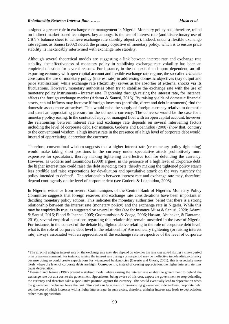
assigned a greater role in exchange rate management in Nigeria. Monetary policy has, therefore, relied

on indirect market-based techniques, key amongst is the use of interest rate (and discretionary use of

CBN’s balance sheet to achieve exchange rate stability objective). Indeed, under a flexible exchange

rate regime, as Sanusi (2002) noted, the primary objective of monetary policy, which is to ensure price

stability, is inextricably intertwined with exchange rate stability.

Although several theoretical models are suggesting a link between interest rate and exchange rate

stability, the effectiveness of monetary policy in stabilising exchange rate volatility has been an

empirical question for several reasons. For instance, in the context of an import-dependent, an oil-

exporting economy with open capital account and flexible exchange rate regime, the so-called trilemma

constrains the use of monetary policy (interest rate) in addressing domestic objectives (say output and

price stabilisation) while exchange rate (flexibility) serves as the absorber of external shocks via its

fluctuations. However, monetary authorities often try to stabilise the exchange rate with the use of

monetary policy instruments - interest rate. Tightening through raising the interest rate, for instance,

affects the foreign exchange market (Adamu & Sanusi, 2016). By raising yields of domestic financial

assets, capital inflows may increase if foreign investors (portfolio, direct and debt instruments) find the

domestic assets more attractive3. This would raise the supply of foreign currency relative to domestic

and exert an appreciating pressure on the domestic currency. The converse would be the case for a

monetary policy easing. In the context of a peg, or managed float with an open capital account, however,

the relationship between interest rate and exchange rate depends on several intervening factors

including the level of corporate debt. For instance, Goderis and Loannidou (2008) show that, contrary

to the conventional wisdom, a high interest rate in the presence of a high level of corporate debt would,

instead of appreciating, depreciate the currency.

Therefore, conventional wisdom suggests that a higher interest rate (or monetary policy tightening)

would make taking short positions in the currency under speculative attack prohibitively more

expensive for speculators, thereby making tightening an effective tool for defending the currency.

However, as Goderis and Loannidou (2008) argues, in the presence of a high level of corporate debt,

the higher interest rate could raise the debt servicing costs, thereby making the tightened policy stance

less credible and raise expectations for devaluation and speculative attack on the very currency the

policy intended to defend4. The relationship between interest rate and exchange rate may, therefore,

depend contingently on the level of corporate debt (see Goderis & Loannidou, 2008).

In Nigeria, evidence from several Communiques of the Central Bank of Nigeria's Monetary Policy

Committee suggests that foreign reserves and exchange rate considerations have been important in

deciding monetary policy actions. This indicates the monetary authorities' belief that there is a strong

relationship between the interest rate (monetary policy) and the exchange rate in Nigeria. While this

may be empirically true, as suggested by several studies (see for instance Musa & Sanusi, 2020; Adamu

& Sanusi, 2016; Flood & Jeanne, 2005; Gudmundsson & Zoega, 2006; Hassan, Abubakar, & Dantama,

2016), several empirical questions regarding this relationship remain unsettled in the case of Nigeria.

For instance, in the context of the debate highlighted above relating to the role of corporate debt level,

what is the role of corporate debt level in the relationship? Are monetary tightening (or raising interest

rate) always associated with an appreciation of the exchange rate irrespective of the level of corporate

3 The effect of a higher interest rate on the exchange rate may also depend on whether the rate was raised during a crises period

or in crises environment. For instance, raising the interest rate during a crises period may be ineffective in defending a currency

because doing so could create expectations for widespread bankruptcies (Basurto and Ghosh, 2001): this is especially more

likely where the level of corporate debts are high. Consequently, instead of causing appreciation, the higher interest rate may

cause depreciation. 4 Bensaid and Jeanne (1997) present a stylised model where raising the interest rate enable the government to defend the

exchange rate but at a cost to the government. Speculators, being aware of this cost, expect the government to stop defending

the currency and therefore take a speculative position against the currency. This would eventually lead to depreciation when

the government no longer bears the cost. This cost can be a result of pre-existing government indebtedness, corporate debt,

etc. the cost of which increases with a higher interest rate. In such a case, therefore, a higher interest rate leads to depreciation,

rather than appreciation.


91

debt? This paper, to the best of our knowledge, is the first attempt to address these empirical questions

in the context of Nigeria.

The rest of the paper is organised as follows: Section 2 reviews the relevant literature. Section 3 presents

the statistical methods of research and describes how the data on commercial banks’ debt level was

generated; section 4 presents and analyses the results; while section 5 concludes the paper.

Literature review

Theoretical framework

Raising the interest rate is a policy tool used by Central Banks to manage exchange rate fluctuations or

defend a currency against a speculative attack in a situation of persistent currency depreciation like the

Naira. This simply refers to adopting a higher interest rate in a tight monetary space to keep existing

investors and maintain their confidence level, and also attract other investors across the globe to

appreciate the currency via capital inflow as well as obtain exchange rate stability. This will minimise

the exposure of economic agents to foreign exchange rate risk in their decision-making process.

The behaviour of exchange rate is determined by many economic fundamentals, but one of the key

fundamental determinants of exchange rate movement from the monetarist perspective as well as the

present global financial setting is the interest rate (Copeland, 2005). However, despite the enormous

theories on exchange rate issues documented in the literature, there is no single theory that provides a

policy framework that fits the dynamics of all nations at every point in time. Therefore, this leaves a

gap for the adoption or adaptation of a theory to serve as a framework for addressing research problems.

Thus, with the recent introduction of the Investors & Exporters FX window which is a more flexible

exchange rate system by the CBN, and policy strategies by the Securities and Exchange Commission

(SEC) to ensure perfect capital mobility in its 2015 to 2025 Capital Market Master Plan5 (CMMP) (such

as, improve market liquidity, improve ease and access of doing business, introduced alternative trading

platforms, create an enabling environment supportive of new products, and facilitate the

internationalization of Nigerian Capital Market), this study, therefore, adopts the Mundell-Flemming

(M-F) model as a theoretical framework. The M-F model in its monetary policy framework explains

how exchange rate behaves (under different exchange rate regimes) in the event of interest rate policy

changes (as a result of changes in the money supply) in a small open economy with perfect capital

mobility (Copeland, 2005)6. Retaining these assumptions, the below headings present a brief policy

picture of the workings of the model.

Monetary expansion, flexible exchange rate and perfect capital mobility in the M-F model

In an open economy, monetary policy is very effective under a flexible exchange rate system. For

example, a monetary expansion would exert downward pressure on the domestic interest rate, thus

leading to capital outflow, domestic currency depreciation, increase in net exports and output and vice

versa for a monetary contraction.

Monetary expansion, fixed exchange rate and perfect capital mobility in the M-F model

In an open economy, monetary policy is not effective under a fixed exchange rate system because of

the monetary authority's commitment to maintaining the exchange rate target, and thus money supply

cannot be affected. The monetary authority maintains the exchange rate target via its intervention in the

foreign exchange market by buying and selling foreign currency in the event of excess demand (due to

capital inflow) and excess supply ( due to capital outflow) of domestic currency respectively. For

example, a monetary expansion would exert downward pressure on the domestic interest rate, thus

leading to capital outflow, domestic currency depreciation and therefore, the monetary authority would

have to sell foreign currency to close the excess supply gap to maintain the exchange rate target. This

would in turn have no beneficial effect on output but a loss in foreign reserves.

5 http://sec.gov.ng/wp-content/uploads/2016/09/PART-A_CCMP.pdf 6 See, Flemming (1962), Mundell (1962), Mundell (1963), Mundell (1968) for original references of the M-F model.

http://sec.gov.ng/wp-content/uploads/2016/09/PART-A_CCMP.pdf


92

Empirical literature

The relationship between high-interest-rate policy and exchange rate or interest rate defence of a

currency has received considerable attention in the international finance literature. A significant

quantum of studies in other countries aside from Nigeria has shown how interest rate policy affects the

exchange rates or speculative attacks on currencies. For instance, Caporale et al. (2005) examined the

effect of monetary tightening on the exchange rate in four Asian countries (The Philippines, Thailand,

South Korea and Indonesia) during Asian crises. Using a bivariate Vector Error Correction Model

(VECM) and data set from 1991:2-2001:10, the study found that monetary tightening helped defend the

currency during periods of tranquillity, however, it showed a reverse effect during the crises.

Chen (2006) used the Markov Switching specification of the nominal exchange rate with time-varying

transition probabilities in four Asian countries (Indonesia, Korea, the Philippines, and Thailand),

Mexico and Turkey. The study utilised weekly data from 03:01:1997 to 30:08:2002 for the four Asian

countries and 07:01:1994 to 30:08:2002 for Mexico. However, monthly data was used for Turkey from

1990:1 to 2002:8. The study founds that raising nominal interest rates leads to a high probability of

switching to a crisis regime. This supports other studies view that high-interest rates may be unable to

defend the exchange rate. Similarly, Bautista (2003) examines interest rate-exchange rate interaction

using dynamic conditional correlation (DCC) analysis – a multivariate Generalized Autoregressive

Conditional Heteroskedasticity (GARCH) method using weekly data for the Philippines from January

1988 to October 2000. The results of the study present evidence of ineffective interest rate defence of

the currency. In addition, Gudmundsson and Zoega (2016) using VECM and monthly data from 2009:1-

2015:2 analysed the effect of interest rate on the exchange rate in Iceland under a capital control regime.

They found that a currency is not likely to depreciate in an effective capital control regime in the event

of cutting interest rates in small steps from a very high level.

Similarly, Flood and Jeanne (2005) derived a model and showed that an interest rate defence of a fixed

exchange rate is effective only if the underlying fiscal situation is sound. That is, if the fiscal condition

is unsound, the currency would be weakened by the harmful effect of the high-interest rate on the public

finances. Also, Goldfajn and Gupta (2003) examined the effectiveness of tight monetary policy in

stabilising exchange rates in the aftermath of currency crises using an unbalanced panel regression

model. They analysed large data sets from 1980-98 for eighty countries. They found that tight monetary

policy facilitates the reversal of currency undervaluation, however, the results are not robust in the

presence of a banking crisis. Goderis and Loannidou (2008) using data from 1986:1-2002:12 for a

sample of countries by constructing a cross-section of large speculative attacks found that a higher

interest rate lowers the probability of a successful speculative attack if the level of short-term corporate

debt is low. Short-term corporate debt was introduced as an additional factor to capture balance sheet

vulnerabilities and to examine if it affects the ability of a monetary policy to defend a fixed exchange

rate.

From the above reviewed studies, it can be seen that the response of the exchange rate to interest rate

policy, though can be linear theoretically, can also be dependent on some additional factors in reality,

such as fiscal soundness, short-term debt level, level of capital mobility and banking crisis. This study

aims to fill the gap in the Nigerian literature by analysing commercial banks debt level as an additional

factor to the relationship.

Moreover, the literature in Nigeria also has documented studies that show how exchange rate responds

to monetary policy or interest rate policy. However, the determinants of exchange rate are also not left

untouched. Mordi (2006) mentioned several economic fundamentals as the determinants of the

exchange rate, some of which are; interest rate movements, inflation, Gross Domestic Product (GDP)

growth rate, external reserves, etc. Having established the strong linkage between interest rate to

exchange rate in Nigeria, several other studies that will follow shows the magnitude and direction of

the response of exchange rate to Monetary or interest rate policy.


93

For instance, Musa and Sanusi (2020) estimated an Autoregressive Distributed Lag model using data

from 1989 to 2017 in Nigeria to examine how the level of capital account openness affect the

relationship between interest rate and exchange rate in Nigeria. They found that an increase in interest

rate depreciates the Naira in the long run regardless of whether the capital account is open or closed but

only if the capital account is open in the short run, however, if the capital account is closed the Naira

appreciates. Thus, the interest rate should be used to manage short-run dynamics of the exchange rate

in addition to effectively enforced capital controls.

Similarly, Adamu and Sanusi (2016) estimated a GARCH (1, 1) model using data for Nigeria from

2007 to 2016 to examine the effect of additional monetary tightening (AMT) on exchange rate volatility

in Nigeria. They found that AMT is effective in reducing exchange rate volatility. In addition, Oke et

al. (2017) examine the relationship between Nigeria's exchange rate, domestic interest rate, and world

interest rate from 1980:Q1 to 2015:Q4 using the VECM estimation technique. Their findings supported

a tightened monetary policy that is not inflationary and economic growth bias in the long run. Ditimi et

al. (2011) using Ordinary Least Square (OLS) technique and data for Nigeria from 1986 to 2009

examined the effect of monetary policy on macroeconomic variables in Nigeria. They found that

monetary policy has a positive significant effect on the exchange rate and a negative significant effect

on the money supply.

Also, Yinusa and Akinlo (2008) used data for Nigeria from 1986:1-2005:2 to estimate a VECM in their

analysis of the implication of currency substitution and exchange rate volatility for monetary policy in

Nigeria. They found that monetary policy may be effective in dampening exchange rate volatility and

currency substitution in the medium horizon but its effectiveness in the short horizon is not certain.

Hassan et al. (2017) examine the sources of exchange rate volatility in Nigeria from 1989:Q1 to

2015:Q4. Using Autoregressive Conditional Heteroskedasticity (ARCH) and ARDL models they found

that, while interest rate and net foreign assets have a positive significant impact on exchange rate

volatility, economic openness, fiscal balance and oil price have an insignificant impact.

Methodology

Model specification

To model the effect of interest rate on the exchange rate in Nigeria and how commercial banks debt

level affects the relationship, we specify a simple equation relating the nominal exchange rate with its

usual theoretical determinants, in line with the interest rate parity hypothesis, the traditional flow model

of Mundell-Fleming and the asset market-based approach to exchange rate determination. Such

variables as the interest rate and income (real GDP) are therefore included on the right-hand side of

equation 1 below (see Castillo, 2002; and Mordi, 2006), in addition to the commercial banks' debt level

(a dummy variable).

𝑙𝑛𝐸𝑋𝐶𝐻 = 𝑓 (𝑀𝑃𝑅, 𝑙𝑛𝑅𝐺𝐷𝑃, 𝐷𝑇 , 𝑀𝑃𝑅 ∗ 𝐷𝑇 , 𝐷99) 1

𝑙𝑛𝐸𝑋𝐶𝐻𝑡 = ɸ0 + ɸ1𝑀𝑃𝑅𝑡 + ɸ2𝑙𝑛𝑅𝐺𝐷𝑃𝑡 + ɸ3𝐷𝑇 + ɸ4𝑀𝑃𝑅𝑡 ∗ 𝐷𝑇 + ɸ5𝐷99 + 𝜇𝑡 2 Where: lnEXCH = log of Exchange rate, MPR = Monetary Policy rate (interest rate), lnRGDP = log

of Real GDP, DT = Dummy variable representing commercial banks debt level with 0 for low debt

level and 1 for high debt level. MPR* DT = interaction dummy between the debt level and MPR, D99 =

Structural dummy which captures the shift to a democratic regime in 1999, with 1 for 1999 and 0 for

all other years. Moreover, we compute Commercial Banks’ Debt level (DT) as7

i. the ratio of Total Debt to Total Assets of Commercial Banks.

ii. the Total Debt is computed as Total Debt = Total Liability - Capital - Total Deposits

(Spaulding, n.d). Where, Total Deposits is the summation of Demand Deposits, Time,

Savings and Foreign Currency Deposits and Central Government Deposits. Note that, Total

Deposits is part of Total Liability but does not form part of Total Debt because the addition

or withdrawal of such Deposits is at the discretion of the depositor. In other words, Deposits

are monies that Banks owe to the depositors.

7 See Appendix 1(Table A2) for the computations and full data.


94

To characterize any Debt level as high or low, it is compared with the sample average of the Total

Debt to Total Assets Ratio. Any Debt level below the sample average is then considered a low Debt

level while those above the average are considered high. This is then used in constructing the

dummy variable DT.

Estimation techniques In this study, we adopt the ARDL bound testing approach developed by (Pesaran et al., 2001) as the

dynamic time series estimation technique to address our research objective. The approach is suitable

for modelling a mixture of both I(1) and I(0) variables except I(2) variables. In addition, it models the

long-run co-movements amongst the variable, it also allows us to incorporate both (long-run)

equilibrium and disequilibrium movements of the exchange rate in the analysis. Thus, we represent the

ARDL form of equation (2) in equation (3) below. The exchange rate is directly quoted such that a

decrease represents appreciation while an increase represents depreciation. Thus, from equation (2), if

any of the coefficients present a negative value (less than zero), that means appreciation and vice versa.

Thus, the a priori expectation of the various parameters/coefficients are as follows; ɸ1 < 0, ɸ2 < 0, ɸ3 >

0, ɸ4 > 0 and ɸ5 > 0.

Δ𝑙𝑛𝐸𝑋𝐶𝐻𝑡 = ɸ0 + ∑ ɸ1

𝑚

𝑖=1Δ𝑙𝑛𝐸𝑋𝐶𝐻𝑡−𝑖 + ∑ ɸ2

𝑚

𝑖=1Δ𝑀𝑃𝑅𝑡−𝑖 + ∑ ɸ3Δ𝑙𝑛𝑅𝐺𝐷𝑃𝑡−𝑖 + 𝛿𝐷𝑇

𝑚

𝑖=1

+ Ω1𝑙𝑛𝐸𝑋𝐶𝐻𝑡−1 + Ω2𝑀𝑃𝑅𝑡−1 + Ω3𝑙𝑛𝑅𝐺𝐷𝑃𝑡−1 + 𝜇𝑡 3

Where 𝜇𝑡 ~𝑖𝑖𝑑(0; 𝛿2), And, m = optimal lag length which is determined using Akaike info Criterion

(AIC), ∆ = first difference of the variables, t = time, t-1= lag one (previous year), ln = natural logarithm,

ɸ0 = constant = summation, ɸ1 to ɸ3, δ and Ω1 to Ω3 are the coefficients of their respective variables and

DT = dummy variable for Debt Levels.

In addition, once it is established that cointegration exists between the variables using bound testing,

the long-run relationship is modelled and estimated as in equation (4) below. In the bound testing

procedure, the null hypothesis of no cointegration is tested against the alternative hypothesis which

establishes the presence of cointegration. F-statistic is used in the decision procedure of the bound

testing approach. The F-statistic is compared against the upper and lower bounds critical values as

tabulated by (Pesaran et al., 2001). If the F-statistic value is above any of the upper bound critical

values, the null hypothesis of no cointegration is rejected and vice versa for the F-statistic value lower

than the lower bound critical values. However, any F-statistic value in between the upper and lower

bound critical values is considered inconclusive.

Δ𝑙𝑛𝐸𝑋𝐶𝐻𝑡 = ɸ0 + Ω1𝑙𝑛𝐸𝑋𝐶𝐻𝑡−1 + Ω2𝑀𝑃𝑅𝑡−1 + Ω3𝑙𝑛𝑅𝐷𝐺𝑃𝑡−1 + 𝛿𝐷𝑇 + 𝜇𝑡 4

While the short-run model is estimated in equation (5) below.

Δ𝑙𝑛𝐸𝑋𝐶𝐻𝑡 = ɸ0 + ∑ ɸ1

𝑛

𝑖=1Δ𝑙𝑛𝐸𝑋𝐶𝐻𝑡−𝑖 + ∑ ɸ2

𝑛

𝑖=1Δ𝑀𝑃𝑅𝑡−𝑖 + ∑ ɸ3Δ𝑙𝑛𝑅𝐺𝐷𝑃𝑡−𝑖 +

𝑛

𝑖=1𝛿𝐷𝑇

+ 𝜗𝐸𝐶𝑇𝑡−𝑖 + 𝜇𝑡 5 Where ECT is the error correction term and ϑ is the speed of convergence towards long-run equilibrium.

Moreover, before the model estimation, a unit root test using Augmented Dickey-Fuller (ADF) and

Phillips-Perron (PP) are performed on all the variables to ascertain the order of integration of the

variables. And finally, after the estimation, the validity of the results is established upon satisfying the

requisite diagnostics and stability test. While Serial correlation, heteroskedasticity, and normality tests

were used for the diagnostics test, the cumulative sums of recursive residuals (CUSUM) and cumulative

sums of squares of recursive residuals (CUSUMSQ) were used for the stability test.

Data, sources and trends

Annual data for the period 1981-2019 on the Exchange Rate, MPR, the Debt level of the banking system

and Real GDP were all collected from the various editions of the Central Bank of Nigeria Statistical

Bulletins8. We, however, constructed a dummy variable that splits the period into that of “high debt”

8 See appendix I (Table A1) for reference to the data.


95

and “low debt”. To do this, we defined any period as a "high debt" period if the debt to asset ratio of

the system is greater than the sample average (see Table A2 of the appendix), hence assign “1” to the

dummy variable, otherwise, we assigned “0”.

To preview the trend relationships to the variables during the period, figures (1) and (2) show the

historical trend of the relationships between Monetary Policy Rate (MPR) and exchange rate, and

between Banks' debt and exchange rate, respectively. Specifically, figure 1 shows that the relationship

between the MPR and exchange rate of the Naira does not appear to depict the expected theoretical link

in most of the period covered. For instance, from 1981 to 1990, 1992 to 1993, 2010 to 2014 and 2016

to 2018, it is evident that as the interest rate (MPR) increased, so does the exchange rate (depreciates).

Similarly, from 2005 to 2007 the exchange rate appreciates (decreased) as the interest rate decreased.

In contrast, it is evident that in 1991, 2000, 2015, and 2019 and also from 1994 to 1998 and 2002 to

2004, as the interest rate decreased, the exchange rate increased (depreciates). Similarly, in 2008 the

exchange rate appreciates (decreased) as the interest rate increased.

Figure 1 Relationship between Monetary Policy Rate and Exchange Rate

Source: computed by authors

Furthermore, figure 2 shows that the Debt level appears to closely move together with the exchange

rate. That is, increases in the debt level appears to be associated with increases (depreciation) in the

exchange rate.

Figure 2. Relationship between Exchange rate and Banks Debt

Source: computed by authors

0

50

100

150

200

250

300

350

0

5

10

15

20

25

30

1981 1983 1985 1987 1989 1991 1993 1995 1997 1999 2001 2003 2005 2007 2009 2011 2013 2015 2017 2019

Relationship between Monetary Policy Rate and Exchange Rate (Right Axis)

Monetary Policy rate Exchange rate

0

5000

10000

15000

20000

0

100

200

300

400

1981 1983 1985 1987 1989 1991 1993 1995 1997 1999 2001 2003 2005 2007 2009 2011 2013 2015 2017 2019

Relationship between Exchange Rate and Banks Debt (Right Axis)

Exchange rate Banks Debt (₦' Billion)


96

Empirical results

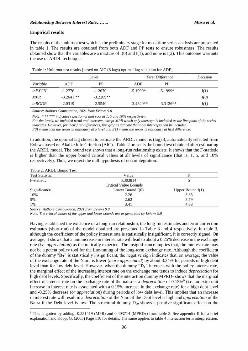
The results of the unit root test which is the preliminary stage for most time series analysis are presented

in table 1. The results are obtained from both ADF and PP tests to ensure robustness. The results

obtained show that the variables are a mixture of I(0) and I(1), and none is I(2). This outcome warrants

the use of ARDL technique.

Table 1: Unit root test results [based on AIC (8 lags) optimal lag selection for ADF]

Level First Difference Decision

Variable ADF PP ADF PP

lnEXCH -1.2776 -1.2670 -5.1999* -5.1999* I(1)

MPR -3.2641 ** -3.2209** I(0)

lnRGDP -2.0319 -2.5540 -3.4340** -3.3126** I(1)

Source: Authors Computation, 2021 from Eviews 9.0

Note: * ** *** indicates rejection of unit root at 1, 5 and 10% respectively.

For the levels, we included trend and intercept, except MPR which only intercept is included as the line plots of the series

indicates. However, for their first differences, line graphs indicate that only intercepts can be included.

I(0) means that the series is stationary at a level and I(1) means the series is stationary at first difference.

In addition, the optimal lag chosen to estimate the ARDL model is (lag) 3, automatically selected from

Eviews based on Akaike Info Criterion (AIC). Table 2 presents the bound test obtained after estimating

the ARDL model. The bound test shows that a long-run relationship exists. It shows that the F-statistic

is higher than the upper bound critical values at all levels of significance (that is, 1, 5, and 10%

respectively). Thus, we reject the null hypothesis of no cointegration.

Table 2: ARDL Bound Test

Test Statistic Value K

F-statistic 5.303814 5

Critical Value Bounds

Significance Lower Bound I(0) Upper Bound I(1)

10% 2.26 3.35

5% 2.62 3.79

1% 3.41 4.68 Source: Authors Computation, 2021 from Eviews 9.0

Note: The critical values of the upper and lower bounds are as generated by Eviews 9.0

Having established the existence of a long-run relationship, the long-run estimates and error correction

estimates (short-run) of the model obtained are presented in Table 3 and 4 respectively. In table 3,

although the coefficient of the policy interest rate is statistically insignificant, it is correctly signed. On

average, it shows that a unit increase in interest rate will lead to about a 0.25% decrease in the exchange

rate (i.e. appreciation) as theoretically expected. The insignificance implies that, the interest rate may

not be a potent policy tool for the fine-tuning of the long-term exchange rate. Although the coefficient

of the dummy "DT” is statistically insignificant, the negative sign indicates that, on average, the value

of the exchange rate of the Naira is lower (more appreciated) by about 3.34% for periods of high debt

level than for low debt level. However, when the dummy “DT" interacts with the policy interest rate,

the marginal effect of the increasing interest rate on the exchange rate tends to induce depreciation for

high debt levels. Specifically, the coefficient of the interaction dummy MPRDT shows that the marginal

effect of interest rate on the exchange rate of the naira is a depreciation of 0.15%9 (i.e. an extra unit

increase in interest rate is associated with a 0.15% increase in the exchange rate) for a high debt level

and -0.25% decrease (or appreciation) during periods of low debt level. This implies that an increase

in interest rate will result in a depreciation of the Naira if the Debt level is high and appreciation of the

Naira if the Debt level is low. The structural dummy D99 shows a positive significant effect on the

9 This is gotten by adding -0.251419 (MPR) and 0.403714 (MPRDT) from table 3. See appendix II for a brief

explanation and Koop, G. (2005) Page 118 for details. The same applies to table 4 interaction term interpretation.


97

exchange rate. This implies that the average exchange rate of the Naira is more depreciated by about

7.23% upon the shift to democratic rule in 1999 as expected. Real GDP is evident to have a positive

significant effect on the exchange rate. This implies that, on average, a 1% increase in Real GDP will

lead to about a 3.91% increase in the exchange rate (i.e. 3.91% depreciation). Although an increase in

Real GDP may expectedly lead to an appreciation of a currency through an increase in net exports

earnings resulting from a high level of production, however, it may also lead to depreciation due rise

in imports through the income effect, particularly if the economy is import-dependent like the case of

Nigeria in our analysis.

Table 3: Estimated Long Run Coefficients using the ARDL approach.

ARDL (1, 0, 1, 2, 0, 1) selected based on AIC. Dependent Variable LNEXCH

Variable Coefficient Std. Error t-Statistic Prob.

MPR -0.251419 0.158275 -1.588490 0.1243

lnRGDP 3.908229 0.404475 9.662470 0.0000

DT -3.344935 2.335890 -1.431975 0.1641

MPR*DT (MPRDT) 0.403714 0.198168 2.037234 0.0519

D99 7.229927 2.198065 3.289223 0.0029

C -34.424095 3.356010 -10.257447 0.0000


Table 4 presents the estimates of the short-run dynamics of the relationship between interest rate and

exchange rate as well as all other exogenous variables in the model. The estimates show that most of

the exogenous variables are statistically significant. The monetary policy rate (interest rate) is shown to

have a statistically significant (negative) appreciating impact on the exchange rate in line with the

conventional wisdom. This implies that, on average, a unit increase in interest rate will lead to about

0.05% decrease (appreciation) in the exchange rate of the Naira. The dummy “DT" is also statistically

insignificant, indicating that, on average, the exchange rate is lower (more appreciated) by about 0.41%

during the period of high debt level than during periods of low debt level. However, when the dummy

“DT" interacts with the policy interest rate, the marginal effect of the increasing interest rate on the

exchange rate tends to be a depreciation in periods of high debt level. Specifically, the interaction

dummy (MPRDT) shows that the marginal effect of interest rate on the exchange rate of the naira is a

depreciation of 0.03% (i.e., -0.05 + 0.08 = 0.03: an extra unit increase in interest rate is associated

with 0.03% increase in the exchange rate) if the Debt level is high and -0.05% decrease (appreciation)

if the Debt level is low. This implies that an increase in interest rate will result in a depreciation of the

Naira in place of a high Debt level and appreciation of the Naira if the Debt level is low.

In addition, the structural dummy D99 shows a positive significant effect on the exchange rate. This

implies that the average exchange rate of the Naira is more depreciated by about 1.23% upon the shift

to democratic rule in 1999 as expected. Real GDP appeared to have a positive but statistically

insignificant impact on the exchange rate. This implies that, on average, a 1% increase in Real GDP

will lead to about 0.41% increase in the exchange rate (i.e. 0.41% depreciation)10.

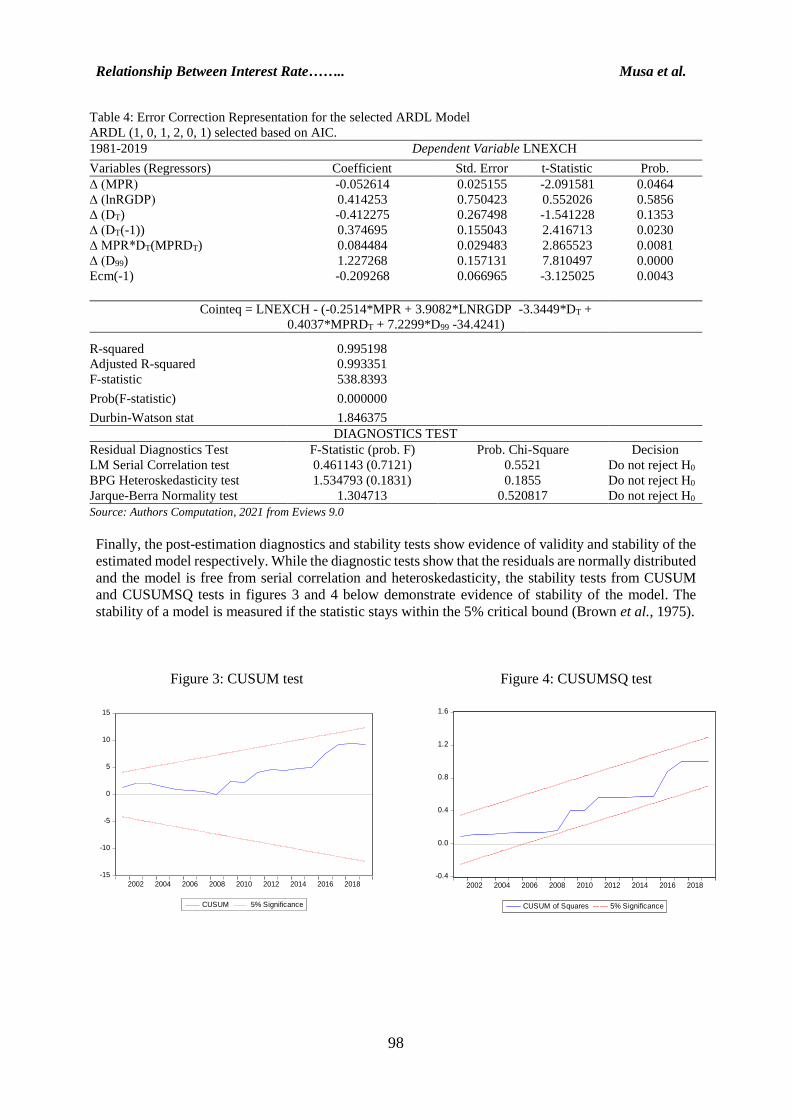
Furthermore, the error correction term (ECM) which measures the speed of adjustment of any

disequilibrium towards a long-run equilibrium state is negative and statistically significant at 1% as

expected. The ECM coefficient of -0.209268 shows about 20.9% convergence to equilibrium in the

long run in one year following a shock.

10 See the analysis of Real GDP in Table 3.


98

Table 4: Error Correction Representation for the selected ARDL Model

ARDL (1, 0, 1, 2, 0, 1) selected based on AIC.

1981-2019 Dependent Variable LNEXCH

Variables (Regressors) Coefficient Std. Error t-Statistic Prob.

∆ (MPR) -0.052614 0.025155 -2.091581 0.0464

∆ (lnRGDP) 0.414253 0.750423 0.552026 0.5856

∆ (DT) -0.412275 0.267498 -1.541228 0.1353

∆ (DT(-1)) 0.374695 0.155043 2.416713 0.0230

∆ MPR*DT(MPRDT) 0.084484 0.029483 2.865523 0.0081

∆ (D99) 1.227268 0.157131 7.810497 0.0000

Ecm(-1) -0.209268 0.066965 -3.125025 0.0043

Cointeq = LNEXCH - (-0.2514*MPR + 3.9082*LNRGDP -3.3449*DT +

0.4037*MPRDT + 7.2299*D99 -34.4241)

R-squared 0.995198

Adjusted R-squared 0.993351

F-statistic 538.8393

Prob(F-statistic) 0.000000

Durbin-Watson stat 1.846375

DIAGNOSTICS TEST

Residual Diagnostics Test F-Statistic (prob. F) Prob. Chi-Square Decision

LM Serial Correlation test 0.461143 (0.7121) 0.5521 Do not reject H0

BPG Heteroskedasticity test 1.534793 (0.1831) 0.1855 Do not reject H0

Jarque-Berra Normality test 1.304713 0.520817 Do not reject H0


Finally, the post-estimation diagnostics and stability tests show evidence of validity and stability of the

estimated model respectively. While the diagnostic tests show that the residuals are normally distributed

and the model is free from serial correlation and heteroskedasticity, the stability tests from CUSUM

and CUSUMSQ tests in figures 3 and 4 below demonstrate evidence of stability of the model. The

stability of a model is measured if the statistic stays within the 5% critical bound (Brown et al., 1975).

Figure 3: CUSUM test Figure 4: CUSUMSQ test

-15

-10

-5

0

5

10

15

2002 2004 2006 2008 2010 2012 2014 2016 2018

CUSUM 5% Significance

-0.4

0.0

0.4

0.8

1.2

1.6

2002 2004 2006 2008 2010 2012 2014 2016 2018

CUSUM of Squares 5% Significance


99

Conclusion and policy implication

The management of exchange rates using monetary policy instruments is inevitable in a contemporary

world of integrated financial markets. However, since in reality, the channel of transmission may not

be smooth and linear as empirically documented from reviewed studies, this study also adds to the

literature by looking at how the exchange rate of the Naira responds to changes in policy interest rates

in the presence of high or low Commercial Banks Debt. The fact being that the banking system is the

largest component of the Nigerian financial system, thus, any shock to it translates to the entire financial

system and the economy at large.

The key findings from this study are that the relationship between exchange rate and interest rate in

Nigeria is, indeed, contingent on the level of Debt of the banking system. Both in the short-run and

long-run, monetary tightening (increase in interest rate) has a depreciating marginal effect on the

exchange rate in the presence of a high Debt level in the banking system. However, in the presence of

a low level of Debt in the banking system, the relationship between the exchange rate and the interest

rate was found to be conventional, such that monetary tightening exert appreciating pressure on the

exchange rate. These findings reveal that, although it may be tempting to raise interest rates to induce

capital inflows and consequently achieve exchange rate appreciation (and reduce inflation, for a given

pass-through), the reverse effect may indeed be the case in the presence of high debt profile in the

banking system. This is because investors may be scared away by the fear of bankruptcy in the system.

This is similar to the findings of (Goderis & Loannidou, 2008).

This finding underscores the potentially important role of corporate Debt levels in determining the

efficacy of monetary policy for exchange rate stabilisation. It is, therefore, recommended that monetary

authorities should keep a close watch on the Debt profile of the banking system, making sure it doesn’t

reach an alarming level.

References Adamu, F.B., & Sanusi, A.R. (2016). Effect of additional monetary tightening on exchange rate volatility in Nigeria.: 2007

– 2016. Researchgate. https://www.researchgate.net/publication/311856015

Basurto, G., Ghosh, A., (2001). The interest rate-exchange rate nexus in currency crises. IMF Staff Papers 47, 99–120.

Bautista, C. C. (2003). Interest rate-exchange rate dynamics in the Philippines: a DCC analysis. Applied Economics Letters,

10(2), 107–111. https://doi.org/10.1080/1350485022000040970

Bensaid, B., & Jeanne, O., (1997). The instability of fixed exchange rate systems when raising the nominal interest rate is

costly. European Economic Review 41, 1461–1478. https://doi.org/10.1016/S0014-2921(96)00022-0

Brown, R., Durbin, J., & Evans, J. (1975). Techniques for testing the constancy of regression relationships over time.

Journal of the Royal Statistical Society. Series B (Methodological), 37(2), 149-192. Retrieved August 19, 2021,

from http://www.jstor.org/stable/2984889

Castillo, G. (2002). Determinants of nominal exchange rate: A survey of the literature, in. Wong, C-H., Khan, M. S., &

Nsouli M. S. (2002) Eds. Macroeconomic Management Programmes and Policies. Chapter 10. International

Monetary Fund. https://doi.org/10.5089/9781589060944.071

Caporale, G. M., Cipollini, A., & Demetriades, P. O. (2005). Monetary policy and the exchange rate during the Asian

crisis: identification through heteroscedasticity. Journal of International Money and Finance, 24(1), 39–53.

https://doi.org/10.1016/j.jimonfin.2004.10.005

CBN (2017). Central Banking at a Glance. Monetary Policy Department.

Chen, S.-S. (2006). Revisiting the interest rate–exchange rate nexus: a Markov-switching approach. Journal of

Development Economics, 79(1), 208–224. https://doi.org/10.1016/j.jdeveco.2004.11.003

Copeland, L. S. (2005). Exchange rate and international finance. London: Pearson Education, Ltd.

Ditimi, A., Nwosa, P.I., & Olaiya, S.A. (2011). An appraisal of monetary policy and its effect on macroeconomic

stabilisation in Nigeria. Journal of Emerging trends in economics and management sciences (JETEMS) 2(3):232-

237.

Fleming J. M. (1962). Domestic financial policies under fixed and floating exchange rates. IMF Staff Papers, 9(3), 369–

380

Flood, R. P., & Jeanne, O. (2005). An interest rate defence of a fixed exchange rate? Journal of International Economics,

66(2), 471–484. https://doi.org/10.1016/j.jinteco.2004.09.001

http://www.jstor.org/stable/2984889

https://doi.org/10.5089/9781589060944.071


100

Goderis, B., & Loannidou, V. P. (2008). Do high-interest rates defend currencies during speculative attacks? New evidence.

Journal of International Economics, 74(1), 158–169. https://doi.org/10.1016/j.jinteco.2007.05.003

Goldfajn, I., & Gupta, P. (2003). Does monetary policy stabilize the exchange rate following a currency crisis? IMF Staff

Papers, 50(1), 90-114.

Gudmundsson, G. S., & Zoega, G. (2016). A double-edged sword: High-interest rates in capital control regimes.

economics: The Open-Access, Open-Assessment E-Journal, 10(2016-17): 1-38.

http://dx.doi.org/10.5018/economics-ejournal.ja.2016-17

Hassan, A., Abubakar, M., & Dantama, Y.U. (2017). Determinants of exchange rate volatility: New estimates from Nigeria.

Eastern Journal of Economics and Finance 3(1), 1-12.

Koop, G. (2005). Analysis of economic data. West Sussex, England: John Wiley & sons ltd.

Moosa, A.I., & Bhatti, H.R. (2010). Theory and empirics of exchange rates. Singapore: World Scientific Publishing Co.

Pte. Ltd.

Mordi, C. N. (2006). Challenges of exchange rate volatility in economic management in Nigeria. CBN Bullion 30(3), 17-

25.

Mundell, R. A. (1962). The appropriate use of monetary and fiscal policy for internal and external stability. IMF Staff

Papers, 9(1), 70-79. https://doi.org/10.2307/3866082

Mundell, R.A. (1963). Capital mobility and stabilization policy under fixed and flexible exchange rates, The Canadian

Journal of Economics and Political Science, 29(4), 475–485. https://doi.org/10.2307/139336

Mundell, R.A. (1968). International Economics, New York: Macmillan.

Musa, A.A., & Sanusi, A.R. (2020). Effect of interest rate on exchange rate management in Nigeria. Nigerian Journal of

Economic and Social Studies, 62(3), 295-313.

Oke, D. M., Bokana, K. G., & Shobande, O. A. (2017). Re-examining the nexus between exchange and interest rates in

Nigeria. Journal of Economics and Behavioural Studies, 9(6), 47-56.

Pesaran, M. H., Shin, Y., & Smith, R. J. (2001). Bounds testing approaches to the analysis of level relationships. Journal

of Applied Econometrics, 16(3), 289–326. Retrieved from http://www.jstor.org/stable/2678547

Sanusi, J. O. (2002). Keynote address. In monetary and exchange rate stability: a Proceeding of a One-day Seminar

organised by the Nigerian Economic Society, held on 23rd May 2002 at Federal Palace Hotel, Lagos. In.

Spaulding, W. C. (n.d.). Bank balance sheet: Assets, liabilities, and bank capital.

https://thismatter.com/money/banking/bank-balance-sheet.htm

Yinusa, D.O., & Akinlo, A.E., (2008). Exchange rate volatility, currency substitution, and monetary policy in Nigeria.

Munich Personal RePEc Archive (MPRA), 16255. Retrieved from https://mpra.ub.uni-muenchen.de/16255

https://doi.org/10.2307/139336

https://thismatter.com/money/banking/bank-balance-sheet.htm


101

Appendix I

Table A1.


102

Table A2. Computation of the Debt level (₦' Billion)

Date(A)

Total liabilities

(B)

Capital

( C )

Total Deposits

(D) Total Debt

=A-B-C

( E )

Total Assets

(F) Total Debt

/Total Assets

(G) AVERAGE of T.debt

to T.assets ratio

(Average of (F))

DUMMY

VALUES

1981 19.4775 0.4974 10.6769 8.3032 19.4775 0.43 0.46 0

1982 22.6619 0.6677 12.0189 9.9753 22.6619 0.44 0.46 0

1983 26.7015 0.8451 13.9385 11.9179 26.7015 0.45 0.46 0

1984 30.0667 0.9667 15.7348 13.3652 30.0667 0.44 0.46 0

1985 31.9979 1.1287 17.5971 13.2721 31.9979 0.41 0.46 0

1986 39.6788 1.2987 18.1376 20.2425 39.6788 0.51 0.46 1

1987 49.8284 1.5451 23.0867 25.1966 49.8284 0.51 0.46 1

1988 58.0272 1.9324 29.0651 27.0297 58.0272 0.47 0.46 1

1989 64.874 2.6923 27.1649 35.0168 64.874 0.54 0.46 1

1990 82.9578 3.7127 38.7773 40.4678 82.9578 0.49 0.46 1

1991 117.5119 4.3008 52.4087 60.8024 117.5119 0.52 0.46 1

1992 159.1908 3.7693 76.0735 79.348 159.1908 0.50 0.46 1

1993 226.1628 4.4202 112.4074 109.3352 226.1628 0.48 0.46 1

1994 295.0332 5.4477 144.0974 145.4881 295.0332 0.49 0.46 1

1995 385.1418 6.5306 182.3856 196.2256 385.1418 0.51 0.46 1

1996 458.7775 8.7305 220.3322 229.7148 458.7775 0.50 0.46 1

1997 584.375 17.6665 280.0289 286.6796 584.375 0.49 0.46 1

1998 694.6151 25.6348 326.9648 342.0155 694.6151 0.49 0.46 1

1999 1070.0198 31.4533 516.7728 521.7937 1070.0198 0.49 0.46 1

2000 1568.8387 44.2057 775.9323 748.7007 1568.8387 0.48 0.46 1

2001 2247.0399 75.1706 975.5253 1196.344 2247.0399 0.53 0.46 1

2002 2766.8803 101.2765 1209.7473 1455.8565 2766.8803 0.53 0.46 1

2003 3047.8563 122.7359 1417.06 1508.0604 3047.8563 0.49 0.46 1

2004 3753.277803 142.3245 1778.713 1832.240303 3753.277803 0.49 0.46 1

2005 4515.11757 172.32152 2155.159834 2187.636216 4515.11757 0.48 0.46 1

2006 7172.932139 170.4948549 3379.275706 3623.161578 7172.932139 0.51 0.46 1

2007 10981.69358 152.9541381 5255.939839 5572.799603 10981.69358 0.51 0.46 1

2008 15919.55982 210.9363277 8252.891781 7455.731716 15919.55982 0.47 0.46 1

2009 17522.85825 219.5099605 9601.809648 7701.53864 17522.85825 0.44 0.46 0

2010 17331.55902 249.7145775 10610.17191 6471.672535 17331.55902 0.37 0.46 0

2011 19396.63376 220.2082421 12131.47043 7044.955083 19396.63376 0.36 0.46 0

2012 21288.14439 188.3876661 14245.08268 6854.674037 21288.14439 0.32 0.46 0

2013 24301.21388 209.621104 16699.05616 7392.536617 24301.21388 0.30 0.46 0

2014 27526.41629 283.3875188 17950.38156 9292.647218 27526.41629 0.34 0.46 0

2015 28173.26094 236.423843 17330.4785 10606.3586 28173.26094 0.38 0.46 0

2016 31682.82367 257.1191975 18394.78676 13030.91771 31682.82367 0.41 0.46 0

2017 34593.8887 275.1145791 19207.14973 15111.6244 34593.8887 0.44 0.46 0

2018 36445.61 277.9 20525.80238 15641.90762 36445.61 0.43 0.46 0

2019 39904.55458 302.1512497 22713.80354 16888.5998 39904.55458 0.42 0.46 0


103

Appendix II

In a regression equation of ƴ = ɸ0 + ɸ1𝐷 + ɸ2𝛽 + ɸ3Ω + 휀 where D is a dummy variable, β is a

continuous variable, Ω is defined as Ω=Dβ and 𝛆 is the random error term. In interpreting the results of

the regression, Ω is 0 for observations with D=0 and β for observations with D=1

Therefore, if D=1 the estimated regression line will be ƴ = ɸ0 + ɸ1 + (ɸ2 + ɸ3)𝛽 and if D=0 the

estimated regression line will be ƴ = ɸ0 + ɸ2𝛽

This implies that the marginal effect of β on ƴ is different for D=0 and D=1 because the regression lines

corresponding to D=0 and D=1 exist with different slopes and intercept.

Documents

RELATIONSHIP BETWEEN INTEREST RATE AND EXCHANGE …