Relational HOG Feature with Wild-Card for Object Detection

Yuji Yamauchi1, Chika Matsushima1, Takayoshi Yamashita2, Hironobu Fujiyoshi11Chubu University, Japan, 2OMRON Corporation, Japan

{yuu, matsu}@vision.cs.chubu.ac.jp, takayosi@omm.ncl.omron.co.jp, hf@cs.chubu.ac.jp

Abstract

This paper proposes Relational HOG (R-HOG) featuresfor object detection, and binary selection by using a wild-card “∗” with Real AdaBoost. HOG features are effectivefor object detection, but their focus on local regions makesthem high-dimensional features. To reduce the memory re-quired for the HOG features, this paper proposes a new fea-ture, R-HOG, which creates binary patterns from the HOGfeatures extracted from two local regions. This approachenables the created binary patterns to reflect the relation-ships between local regions. Furthermore, we extend the R-HOG features by shifting the gradient orientations. Theseshifted Relational HOG (SR-HOG) features make it possi-ble to clarify the size relationships of the HOG features.However, since R-HOG and SR-HOG features contain bi-nary values not needed for classification, we have added aprocess to the Real AdaBoost learning algorithm in which“∗” permits either of the two binary values “0” and “1”,and so valid binary values can be selected. Evaluation ex-periment demonstrated that the SR-HOG features introduc-ing “∗” offers better detection performance than the con-ventional method (HOG feature) despite the reduced mem-ory requirements.

1. IntroductionWith the increasing use of digital cameras and vehicle-

mounted cameras, the expectations for practical detectionof humans in image for the purposes of improving imagequality and assisting the drivers of vehicles are also rising.Research on the use of Field Programmable Gate Arrays(FPGA) or other such hardware implementations of thatfunction has been done [12, 3, 6]. In hardware implementa-tions, it is important that the detection method can operatewith high accuracy, high-speed and low memory require-ments.

Most detection methods proposed in recent years usecombinations of local features of images and stochasticlearning [2, 18, 7, 15, 17]. Local region gradients [5, 1],which are used as features in many proposals, can capture

the shape of an object, but very many dimensions are re-quired to obtain the features of each local region. The diffi-culty of accomplishing that with small-scale hardware thathas limited memory is a major problem whose solution re-quires a reduction in the amount of feature data. Less datahas two benefits. One is that less memory is needed and theother is that features can be categorical, each representingcommon properties.

Two approaches to reducing the amount of data can beconsidered: compressing the feature space to reduce thenumber of features and reducing the amount of data neededfor each feature. The former approach includes methodssuch as vector quantization to reduce the number of fea-tures [9] and principle component analysis to compress thefeature dimensions. These methods can retain the originalamount of data while reducing the number of feature dimen-sions. Human detection, however, involves the processingof a huge number of detection windows, so these methodsare very inefficient.

The latter approach involves quantizing features at a lowbit rate. Scalar quantization, for example, can represent thefeature data at a bit rate that fits the problem. Quantiza-tion is also an effective way to reduce the amount of data.In addition to representing the information with the mini-mum amount of data, it has the advantages of being robustagainst noise and easy to use. One method of quantizationis threshold processing, which is simple and has the advan-tage of low computational cost. However, determining theoptimum threshold for many samples is difficult. Anotherbinarization method uses the size relationship. The LocalBinary Pattern (LBP) proposed by Ojala etal. [13, 16, 11]and a method that expands on that [4] have the advantage ofnot requiring a threshold, as binarization is based on com-parison of the two values. Threshold binarization and sizerelationship binarization also differ in the data contained inone binary value. In threshold processing, the value repre-sents only size, but when size relationship is used, the rela-tion between two values is also included.

Our method focuses on binarization using the size re-lationship, which is one of the latter methods of reducingdata quantity. To achieve highly accurate object detection

2011 IEEE International Conference on Computer Vision Workshops978-1-4673-0063-6/11/$26.00 c©2011 IEEE

1785

while reducing the amount of feature data, we propose theRelational HOG (R-HOG) feature, a binarization method inwhich the size relationship is obtained by comparing HOGfeatures from two local regions. Since R-HOG features usesthe size relationship of two HOG features, they can repre-sent the relatedness of local regions. However, they com-bine multiple binary values, and so contain values that areunnecessary for classification. We solved that problem byintroducing a wild-card “∗”, which permits either of the twobinary values of “0” and “1”, when training. That makesit possible to select the binary values that are effective forclassification by Real AdaBoost.

2. Related works

Local Binary Patterns (LBP) are a technique that is beingapplied in a variety of fields such as object detection, facerecognition, and action recognition. The LBP features pro-posed by Ojala et al. [13] represent the magnitude relationsof a pixel to adjacent pixels with a code, thus allowing rep-resentations of fixed shapes such as edges. Liao et al. pro-posed a method for application to face recognition in whichLBP is extended to represent magnitude relations betweenthe average luminance values in multi-resolution block ar-eas [8]. Another technique applied in face recognition[14]and action recognition [20] is the Local Ternary Pattern(LTP), which extends LBP by using three values for thethreshold. Although that method can capture the relationsof nearby and adjacent pixels, it cannot represent other ef-fective combinations that exist. Furthermore, the LTP ap-proach requires optimum values for the three thresholds.

Methods that combine multiple feature quantities in-clude the Joint Haar-like features proposed by Mita et al.,which capture the relations of Haar-like features in differ-ent positions [10], and co-occurrence features that link theoutput values of weak classifiers with operators proposed byYamauchi et al. [19]. These methods combine feature quan-tities on the basis of recognition results, so the combinationof features may be negatively affected when the results arein error or when the target of detection is obscured.

In contrast to those methods, the features that we pro-pose capture the relations of local gradients, and can thuscapture the relationships with all areas rather than simplyneighboring areas as in LBP and LTP. Furthermore, usingthe wild-card character “∗” has a masking effect in whichbinaries that are not needed for distinguishing the target arenot observed. It is therefore possible to use only the bina-ries that are effective for discrimination, and approach thatcan be expected to suppress degradation of recognition ac-curacy.

3. HOG features and binarizationThis section describes HOG features and binarization as

means of reducing the amount of HOG feature data.

3.1. HOG features

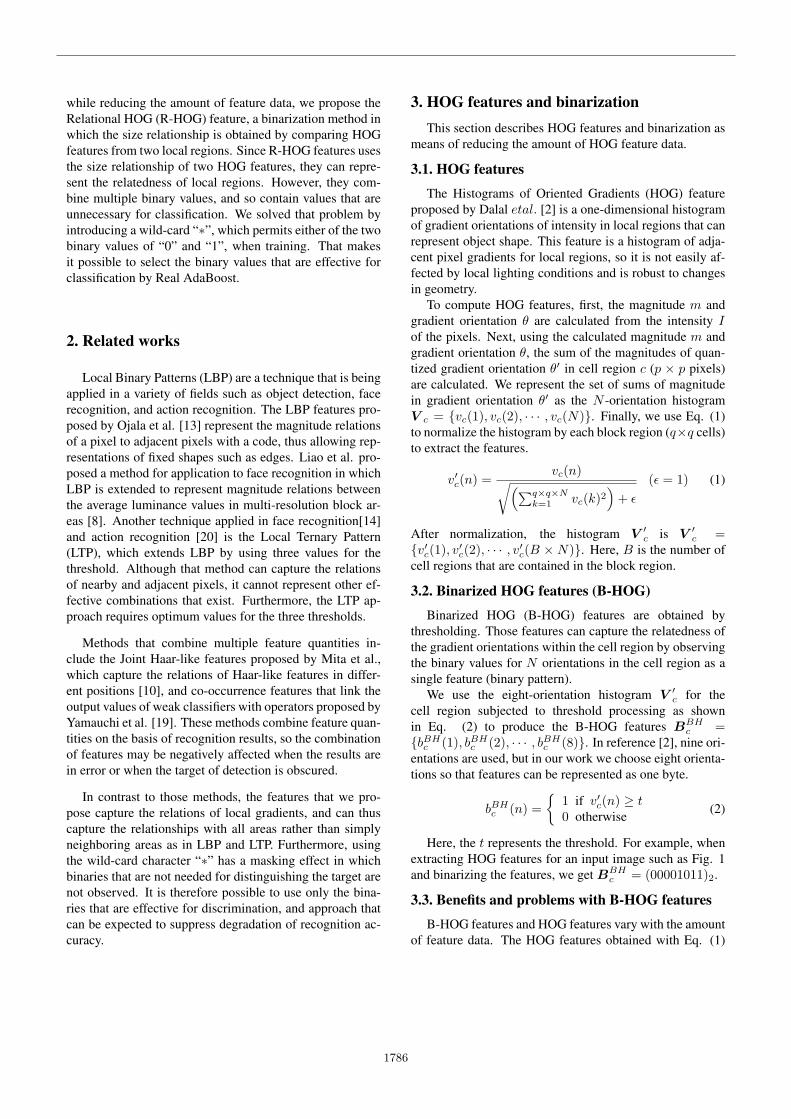
The Histograms of Oriented Gradients (HOG) featureproposed by Dalal etal. [2] is a one-dimensional histogramof gradient orientations of intensity in local regions that canrepresent object shape. This feature is a histogram of adja-cent pixel gradients for local regions, so it is not easily af-fected by local lighting conditions and is robust to changesin geometry.

To compute HOG features, first, the magnitude m andgradient orientation θ are calculated from the intensity Iof the pixels. Next, using the calculated magnitude m andgradient orientation θ, the sum of the magnitudes of quan-tized gradient orientation θ′ in cell region c (p × p pixels)are calculated. We represent the set of sums of magnitudein gradient orientation θ′ as the N -orientation histogramV c = {vc(1), vc(2), · · · , vc(N)}. Finally, we use Eq. (1)to normalize the histogram by each block region (q×q cells)to extract the features.

v′c(n) =

vc(n)√(∑q×q×Nk=1 vc(k)2

)+ ϵ

(ϵ = 1) (1)

After normalization, the histogram V ′c is V ′

c ={v′

c(1), v′c(2), · · · , v′c(B × N)}. Here, B is the number of

cell regions that are contained in the block region.

3.2. Binarized HOG features (B-HOG)

Binarized HOG (B-HOG) features are obtained bythresholding. Those features can capture the relatedness ofthe gradient orientations within the cell region by observingthe binary values for N orientations in the cell region as asingle feature (binary pattern).

We use the eight-orientation histogram V ′c for the

cell region subjected to threshold processing as shownin Eq. (2) to produce the B-HOG features BBH

c ={bBH

c (1), bBHc (2), · · · , bBH

c (8)}. In reference [2], nine ori-entations are used, but in our work we choose eight orienta-tions so that features can be represented as one byte.

bBHc (n) =

{1 if v′

c(n) ≥ t0 otherwise (2)

Here, the t represents the threshold. For example, whenextracting HOG features for an input image such as Fig. 1and binarizing the features, we get BBH

c = (00001011)2.

3.3. Benefits and problems with B-HOG features

B-HOG features and HOG features vary with the amountof feature data. The HOG features obtained with Eq. (1)

1786

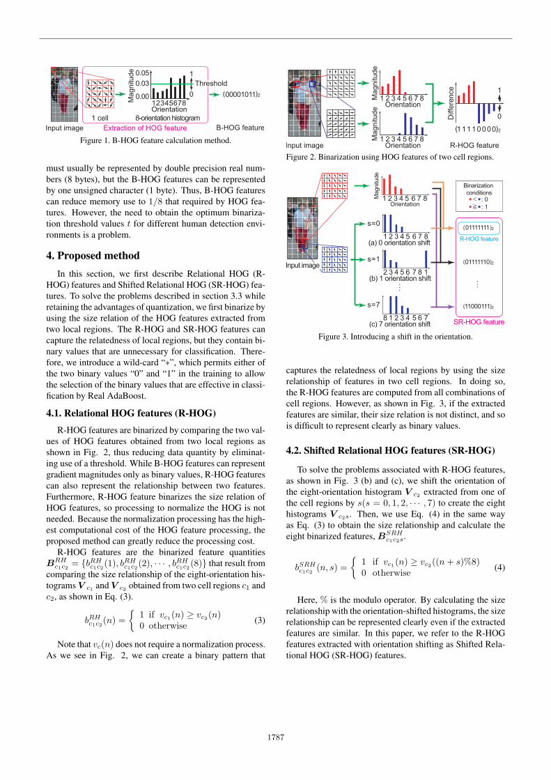
Figure 1. B-HOG feature calculation method.

must usually be represented by double precision real num-bers (8 bytes), but the B-HOG features can be representedby one unsigned character (1 byte). Thus, B-HOG featurescan reduce memory use to 1/8 that required by HOG fea-tures. However, the need to obtain the optimum binariza-tion threshold values t for different human detection envi-ronments is a problem.

4. Proposed methodIn this section, we first describe Relational HOG (R-

HOG) features and Shifted Relational HOG (SR-HOG) fea-tures. To solve the problems described in section 3.3 whileretaining the advantages of quantization, we first binarize byusing the size relation of the HOG features extracted fromtwo local regions. The R-HOG and SR-HOG features cancapture the relatedness of local regions, but they contain bi-nary values that are unnecessary for classification. There-fore, we introduce a wild-card “∗”, which permits either ofthe two binary values “0” and “1” in the training to allowthe selection of the binary values that are effective in classi-fication by Real AdaBoost.

4.1. Relational HOG features (R-HOG)

R-HOG features are binarized by comparing the two val-ues of HOG features obtained from two local regions asshown in Fig. 2, thus reducing data quantity by eliminat-ing use of a threshold. While B-HOG features can representgradient magnitudes only as binary values, R-HOG featurescan also represent the relationship between two features.Furthermore, R-HOG feature binarizes the size relation ofHOG features, so processing to normalize the HOG is notneeded. Because the normalization processing has the high-est computational cost of the HOG feature processing, theproposed method can greatly reduce the processing cost.

R-HOG features are the binarized feature quantitiesBRH

c1c2= {bRH

c1c2(1), bRH

c1c2(2), · · · , bRH

c1c2(8)} that result from

comparing the size relationship of the eight-orientation his-tograms V c1 and V c2 obtained from two cell regions c1 andc2, as shown in Eq. (3).

bRHc1c2

(n) ={

1 if vc1(n) ≥ vc2(n)0 otherwise (3)

Note that vc(n) does not require a normalization process.As we see in Fig. 2, we can create a binary pattern that

Figure 2. Binarization using HOG features of two cell regions.

Figure 3. Introducing a shift in the orientation.

captures the relatedness of local regions by using the sizerelationship of features in two cell regions. In doing so,the R-HOG features are computed from all combinations ofcell regions. However, as shown in Fig. 3, if the extractedfeatures are similar, their size relation is not distinct, and sois difficult to represent clearly as binary values.

4.2. Shifted Relational HOG features (SR-HOG)

To solve the problems associated with R-HOG features,as shown in Fig. 3 (b) and (c), we shift the orientation ofthe eight-orientation histogram V c2 extracted from one ofthe cell regions by s(s = 0, 1, 2, · · · , 7) to create the eighthistograms V c2s. Then, we use Eq. (4) in the same wayas Eq. (3) to obtain the size relationship and calculate theeight binarized features, BSRH

c1c2s.

bSRHc1c2

(n, s) ={

1 if vc1(n) ≥ vc2((n + s)%8)0 otherwise (4)

Here, % is the modulo operator. By calculating the sizerelationship with the orientation-shifted histograms, the sizerelationship can be represented clearly even if the extractedfeatures are similar. In this paper, we refer to the R-HOGfeatures extracted with orientation shifting as Shifted Rela-tional HOG (SR-HOG) features.

1787

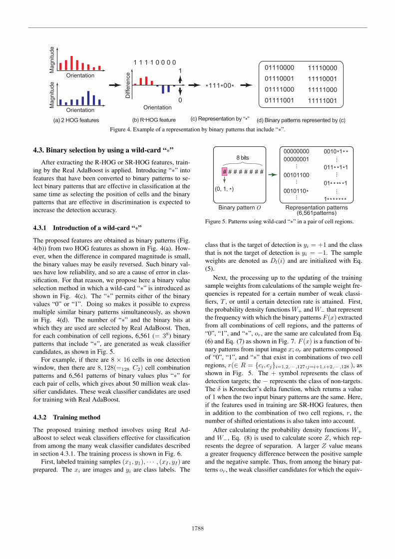
Figure 4. Example of a representation by binary patterns that include “∗”.

4.3. Binary selection by using a wild-card “∗”

After extracting the R-HOG or SR-HOG features, train-ing by the Real AdaBoost is applied. Introducing “∗” intofeatures that have been converted to binary patterns to se-lect binary patterns that are effective in classification at thesame time as selecting the position of cells and the binarypatterns that are effective in discrimination is expected toincrease the detection accuracy.

4.3.1 Introduction of a wild-card “∗”

The proposed features are obtained as binary patterns (Fig.4(b)) from two HOG features as shown in Fig. 4(a). How-ever, when the difference in compared magnitude is small,the binary values may be easily reversed. Such binary val-ues have low reliability, and so are a cause of error in clas-sification. For that reason, we propose here a binary valueselection method in which a wild-card “∗” is introduced asshown in Fig. 4(c). The “∗” permits either of the binaryvalues “0” or “1”. Doing so makes it possible to expressmultiple similar binary patterns simultaneously, as shownin Fig. 4(d). The number of “∗” and the binary bits atwhich they are used are selected by Real AdaBoost. Then,for each combination of cell regions, 6,561 (= 38) binarypatterns that include “∗”, are generated as weak classifiercandidates, as shown in Fig. 5.

For example, if there are 8 × 16 cells in one detectionwindow, then there are 8, 128(=128 C2) cell combinationpatterns and 6,561 patterns of binary values plus “∗” foreach pair of cells, which gives about 50 million weak clas-sifier candidates. These weak classifier candidates are usedfor training with Real AdaBoost.

4.3.2 Training method

The proposed training method involves using Real Ad-aBoost to select weak classifiers effective for classificationfrom among the many weak classifier candidates describedin section 4.3.1. The training process is shown in Fig. 6.

First, labeled training samples (x1, y1), · · · , (xI , yI) areprepared. The xi are images and yi are class labels. The

Figure 5. Patterns using wild-card “∗” in a pair of cell regions.

class that is the target of detection is yi = +1 and the classthat is not the target of detection is yi = −1. The sampleweights are denoted as Dl(i) and are initialized with Eq.(5).

Next, the processing up to the updating of the trainingsample weights from calculations of the sample weight fre-quencies is repeated for a certain number of weak classi-fiers, T , or until a certain detection rate is attained. First,the probability density functions W+ and W− that representthe frequency with which the binary patterns F (x) extractedfrom all combinations of cell regions, and the patterns of“0”, “1”, and “∗”, or, are the same are calculated from Eq.(6) and Eq. (7) as shown in Fig. 7. F (x) is a function of bi-nary patterns from input image x; or are patterns composedof “0”, “1”, and “∗” that exist in combinations of two cellregions, r(∈ R = {ci, cj}i=1,2,··· ,127,j=i+1,i+2,··· ,128 ), asshown in Fig. 5. The + symbol represents the class ofdetection targets; the − represents the class of non-targets.The δ is Kronecker’s delta function, which returns a valueof 1 when the two input binary patterns are the same. Here,if the features used in training are SR-HOG features, thenin addition to the combination of two cell regions, r, thenumber of shifted orientations is also taken into account.

After calculating the probability density functions W+

and W−, Eq. (8) is used to calculate score Z, which rep-resents the degree of separation. A larger Z value meansa greater frequency difference between the positive sampleand the negative sample. Thus, from among the binary pat-terns or, the weak classifier candidates for which the equiv-

1788

¶ ³1, Input: Labeled training samples I .

{xi, yi}i=1···I , yi ∈ {−1, 1}2, Initialization: Initialization of sample weights.

D1(i) = 1/I (5)3, Training:

For l = 1, · · · , L //Number of weak classifiers.For r = 1, · · · , R //Combination number of two cell regions.

For o = 1, · · · , O //Binary pattern with wild-card “∗”.

· Calculate the probability density functions.W+ =

X

i:yi=+1

Dl(i)δ[F (xi), or] (6)

W− =X

i:yi=−1

Dl(i)δ[F (xi), or] (7)

· Calculate the score Z.Zor = |W+ − W−| (8)

End forEnd for

· Select weak classifier hl.hl = arg max

or∈(O×R)Zor (9)

· Update sample weights.Dl+1(i) = Dl(i) exp [−yihl(xi)] (10)

h(xi) =

8

<

:

12

lnW++ϵ

W−+ϵif F (xi) = or

12

ln(1−W+)+ϵ

(1−W−)+ϵotherwise

(11)

End for

4, Output: Strong classifier.

H(x) = sign

"

LX

l=1

hl(x)

#

(12)

µ ´Figure 6. Training algorithm.

Figure 7. Calculation of the probability density functions.

alent value Z from Eq. (9) is maximum are selected as theeffective weak classifiers for round l, hl.

After selection of the weak classifiers, Eq. (10) is used toupdate the training sample weights so that the training sam-ples that failed to classify will classify correctly in the nextround. Then, the probability density functions of the se-lected weak classifier sample, W+ and W−, are used to cal-culate the weak classifier output hl(x) from Eq. (9). Here,the W+ and (1 − W+) and the W− and (1 − W−) are nor-

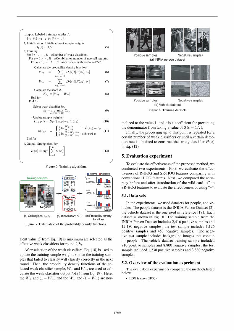
Figure 8. Training datasets.

malized to the value 1, and ϵ is a coefficient for preventingthe denominator from taking a value of 0 (ϵ = 1/I).

Finally, the processing up to this point is repeated for acertain number of weak classifiers or until a certain detec-tion rate is obtained to construct the strong classifier H(x)in Eq. (12).

5. Evaluation experimentTo evaluate the effectiveness of the proposed method, we

conducted two experiments. First, we evaluate the effec-tiveness of R-HOG and SR-HOG features comparing withconventional HOG features. Next, we compared the accu-racy before and after introduction of the wild-card “∗” toSR-HOG features to evaluate the effectiveness of using “∗”.

5.1. Data sets

In the experiments, we used datasets for people, and ve-hicles. The people dataset is the INRIA Person Dataset [2];the vehicle dataset is the one used in reference [19]. Eachdataset is shown in Fig. 8. The training sample from theINRIA Person Dataset includes 2,416 positive samples and12,180 negative samples; the test sample includes 1,126positive samples and 453 negative samples. The nega-tive test sample includes background images that containno people. The vehicle dataset training sample included710 positive samples and 8,800 negative samples; the testsample included 1,230 positive samples and 3,880 negativesamples.

5.2. Overview of the evaluation experimentThe evaluation experiments compared the methods listed

below.• HOG features (HOG)

1789

Dataset Image size Cell size Block size Orientation[pix.] [pix.] [cell]

INRIA[2] 64 × 128 8 × 8 2 × 2 8Vehicle[19] 72 × 54 9 × 9 2 × 2 8

Table 1. Parameters used in the experiment for each dataset.

• Binarized HOG features (B-HOG)

• Relational HOG features (R-HOG)

• R-HOG features + shifted-orientation (SR-HOG)

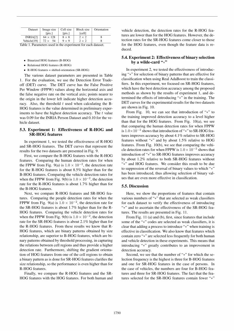
The various dataset parameters are presented in Table1. For the evaluation, we use the Detection Error Trade-off (DET) curve. The DET curve has the False PositivePer Window (FPPW) values along the horizontal axis andthe false negative rate on the vertical axis; points nearer tothe origin in the lower left indicate higher detection accu-racy. Also, the threshold t used when calculating the B-HOG features is the value determined in preliminary exper-iments to have the highest detection accuracy. The t valuewas 0.09 for the INRIA Person Dataset and 0.10 for the ve-hicle dataset.

5.3. Experiment 1: Effectiveness of R-HOG andSR-HOG features

In experiment 1, we tested the effectiveness of R-HOGand SR-HOG features. The DET curves that represent theresults for the two datasets are presented in Fig. 9.

First, we compare the B-HOG features with the R-HOGfeatures. Comparing the human detection rates for whenthe FPPW from Fig. 9(a) is 1.0 × 10−2, the detection ratefor the R-HOG features is about 8.5% higher than for theB-HOG features. Comparing the vehicle detection rates forwhen the FPPW from Fig. 9(b) is 1.0× 10−2, the detectionrate for the R-HOG features is about 1.7% higher than forthe B-HOG features.

Next, we compare R-HOG features and SR-HOG fea-tures. Comparing the people detection rates for when theFPPW from Fig. 9(a) is 1.0 × 10−2, the detection rate forthe SR-HOG features is about 1.7% higher than for the R-HOG features. Comparing the vehicle detection rates forwhen the FPPW from Fig. 9(b) is 1.0× 10−2, the detectionrate for the SR-HOG features is about 2.1% higher than forthe R-HOG features. From these results we know that R-HOG features, which are binary patterns obtained by sizerelationship, are superior to B-HOG features, which are bi-nary patterns obtained by threshold processing, in capturingthe relations between cell regions and thus provide a higherdetection rate. Furthermore, shifting the gradient orienta-tion of HOG features from one of the cell regions to obtaina binary pattern as is done for SR-HOG features clarifies thesize relationship, so the performance is even higher than forR-HOG features.

Finally, we compare the R-HOG features and the SR-HOG features with the HOG features. For both human and

vehicle detection, the detection rates for the R-HOG fea-tures are lower than for the HOG features. However, the de-tection rates for the SR-HOG features come closer to thosefor the HOG features, even though the feature data is re-duced.

5.4. Experiment 2: Effectiveness of binary selectionby a wilde-card “∗”

In experiment 2, we tested the effectiveness of introduc-ing “∗” for selection of binary patterns that are effective forclassification when using Real AdaBoost to train the classi-fiers. In this experiment, we focused on SR-HOG features,which have the best detection accuracy among the proposedmethods as shown by the results of experiment 1, and de-termined the effects of introducing “∗” in the training. TheDET curves for the experimental results for the two datasetsare shown in Fig. 10.

From Fig. 10, we can see that introduction of “∗” tothe training improved detection accuracy to a level higherthan that for the HOG features. From Fig. 10(a), we seethat comparing the human detection rates for when FPPWis 1.0×10−2 shows that introduction of “∗” to SR-HOG fea-tures improves accuracy by about 4.1% relative to SR-HOGfeatures without “∗” and by about 1.5% relative to HOGfeatures. From Fig. 10(b), we see that comparing the vehi-cle detection rates for when FPPW is 1.0×10−2 shows thatintroduction of “∗” to SR-HOG features improves accuracyby about 1.2% relative to both SR-HOG features without“∗” and HOG features. We consider this result to be dueto suppression of the reversal of binary values to which “∗”has been introduced, thus allowing selection of binary val-ues that are even more effective in classification.

5.5. Discussion

Here, we show the proportions of features that containvarious numbers of “∗” that are selected as weak classifiersfor each dataset to verify the effectiveness of introducing“∗” and to ascertain the effectiveness of the SR-HOG fea-tures. The results are presented in Fig. 11.

From Fig. 11 (a) and (b), first, since features that includesome of the “∗” codes are selected as weak classifiers, it isclear that adding a process to introduce “∗” when training iseffective in classification. We also know that features whichcontain zero “∗” are selected less frequently for both humanand vehicle detection in these experiments. This means thatintroducing “∗” greatly contributes to an improvement indetection accuracy.

Second, we see that the number of “∗” for which the se-lection frequency is the highest is three for B-HOG featuresand one for SR-HOG features in the case of persons. Inthe case of vehicles, the numbers are four for B-HOG fea-tures and three for SR-HOG features. The fact that the fea-tures selected for the SR-HOG features contain fewer “∗”

1790

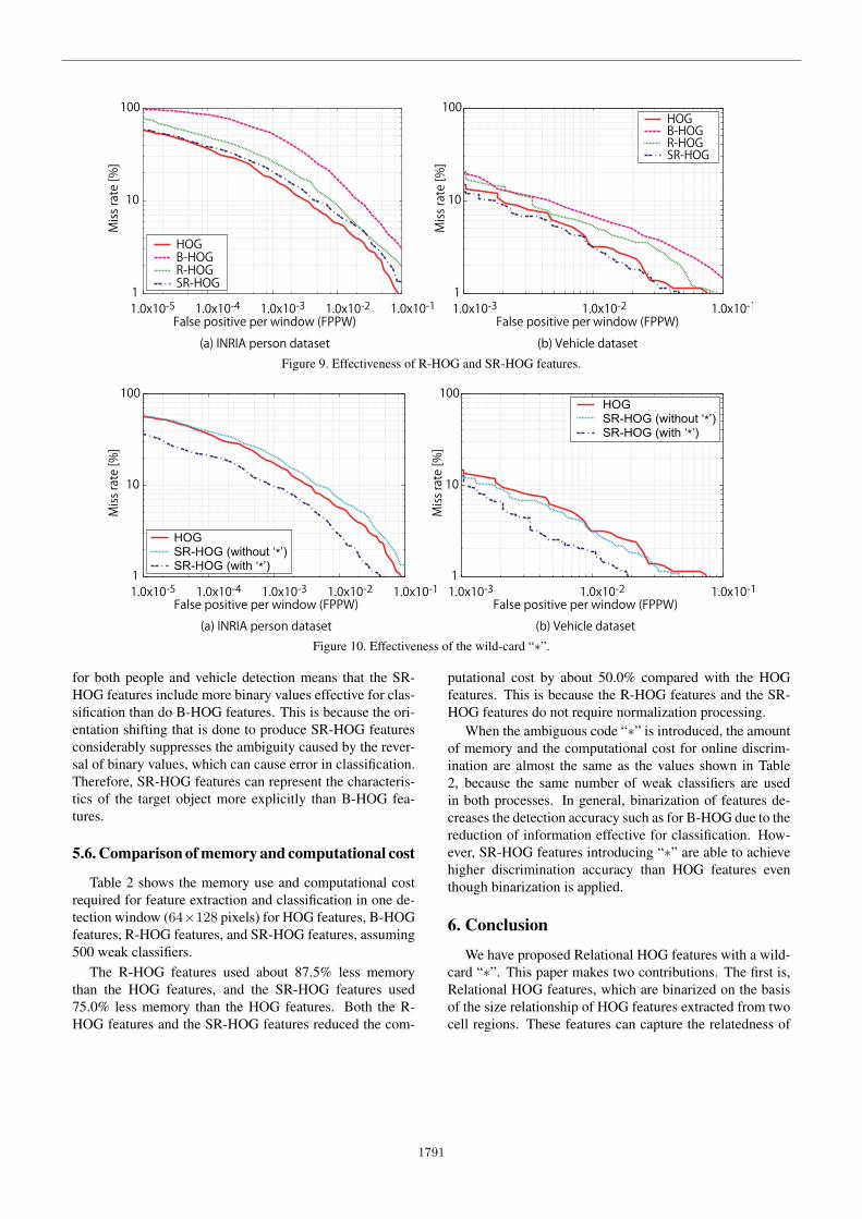
Figure 9. Effectiveness of R-HOG and SR-HOG features.

Figure 10. Effectiveness of the wild-card “∗”.

for both people and vehicle detection means that the SR-HOG features include more binary values effective for clas-sification than do B-HOG features. This is because the ori-entation shifting that is done to produce SR-HOG featuresconsiderably suppresses the ambiguity caused by the rever-sal of binary values, which can cause error in classification.Therefore, SR-HOG features can represent the characteris-tics of the target object more explicitly than B-HOG fea-tures.

5.6. Comparison of memory and computational cost

Table 2 shows the memory use and computational costrequired for feature extraction and classification in one de-tection window (64×128 pixels) for HOG features, B-HOGfeatures, R-HOG features, and SR-HOG features, assuming500 weak classifiers.

The R-HOG features used about 87.5% less memorythan the HOG features, and the SR-HOG features used75.0% less memory than the HOG features. Both the R-HOG features and the SR-HOG features reduced the com-

putational cost by about 50.0% compared with the HOGfeatures. This is because the R-HOG features and the SR-HOG features do not require normalization processing.

When the ambiguous code “∗” is introduced, the amountof memory and the computational cost for online discrim-ination are almost the same as the values shown in Table2, because the same number of weak classifiers are usedin both processes. In general, binarization of features de-creases the detection accuracy such as for B-HOG due to thereduction of information effective for classification. How-ever, SR-HOG features introducing “∗” are able to achievehigher discrimination accuracy than HOG features eventhough binarization is applied.

6. Conclusion

We have proposed Relational HOG features with a wild-card “∗”. This paper makes two contributions. The first is,Relational HOG features, which are binarized on the basisof the size relationship of HOG features extracted from twocell regions. These features can capture the relatedness of

1791

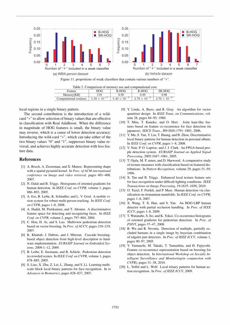
Figure 11. proportions of weak classifiers that contain various numbers of “∗”.

Table 2. Comparison of memory use and computational cost.Feature HOG B-HOG R-HOG SR-HOG

Memory[KB] 3.91 0.50 0.49 0.98Computational cost[ms] 5.39 × 10−7 5.40 × 10−7 2.70 × 10−7 2.70 × 10−7

local regions in a single binary pattern.The second contribution is the introduction of a wild-

card “∗” to allow selection of binary values that are effectivein classification with Real AdaBoost. When the differencein magnitude of HOG features is small, the binary valuemay reverse, which is a cause of lower detection accuracy.Introducing the wild-card “∗”, which can take either of thetwo binary values “0” and “1”, suppresses binary value re-versal, and achieves highly accurate detection with less fea-ture data.

References[1] A. Bosch, A. Zisserman, and X. Munoz. Representing shape

with a spatial pyramid kernel. In Proc. of ACM internationalconference on Image and video retrieval, pages 401–408,2007.

[2] N. Dalal and B. Triggs. Histograms of oriented gradients forhuman detection. In IEEE Conf. on CVPR, volume 1, pages886–893, 2005.

[3] A. Ess, B. Leibe, K. Schindler, and L. V. Gool. A mobile vi-sion system for robust multi-person tracking. In IEEE Conf.on CVPR, pages 1–8, 2008.

[4] A. Hadid, M. Pietikainen, and T. Ahonen. A discriminativefeature space for detecting and recognizing faces. In IEEEConf. on CVPR, volume 2, pages 797–804, 2004.

[5] C. Hou, H. Ai, and S. Lao. Multiview pedestrian detectionbased on vector boosting. In Proc. of ACCV, pages 210–219,2007.

[6] K. Khattab, J. Dubois, and J. Miteran. Cascade boosting-based object detection from high-level description to hard-ware implementation. EURASIP Journal on Embedded Sys-tems, 2009:1–12, 2009.

[7] B. Leibe, E. Seemann, and B. Schiele. Pedestrian detectionin crowded scenes. In IEEE Conf. on CVPR, volume 1, pages878–885, 2005.

[8] S. Liao, X. Zhu, Z. Lei, L. Zhang, and S. Li. Learning multi-scale block local binary patterns for face recognition. In inAdvances in Biometrics, pages 828–837, 2007.

[9] Y. Linde, A. Buzo, and R. Gray. An algorithm for vectorquantizer design. In IEEE Trans. on Communications, vol-ume 28, pages 84–95, 1980.

[10] T. Mita, T. Kaneko, and O. Hori. Joint haar-like fea-tures based on feature co-occurrence for face detection (injapanese). IEICE Trans., J89-D(8):1791–1801, 2006.

[11] Y. Mu, S. Yan, Y. Liu, T. Huang, and B. Zhou. Discriminativelocal binary patterns for human detection in personal album.In IEEE Conf. on CVPR, pages 1–8, 2008.

[12] V. Nair, P. O. Laprise, and J. J. Clark. An FPGA-based peo-ple detection system. EURASIP Journal on Applied SignalProcessing, 2005:1047–1061, 2005.

[13] T. Ojala, M. P. ainen, and D. Harwood. A comparative studyof texture measures with classification based on featured dis-tributions. In Pattern Recognition, volume 29, pages 51–59,1996.

[14] X. Tan and B. Triggs. Enhanced local texture feature setsfor face recognition under difficult lighting conditions. IEEETransactions on Image Processing, 19:1635–1650, 2010.

[15] O. Tuzel, F. Porikli, and P. Meer. Human detection via clas-sification on riemannian manifolds. In IEEE Conf. on CVPR,pages 1–8, 2007.

[16] X. Wang, T. X. Han, and S. Yan. An HOG-LBP humandetector with partial occlusion handling. In Proc. of IEEEICCV, pages 1–8, 2009.

[17] T. Watanabe, S. Ito, and K. Yokoi. Co-occurrence histogramsof oriented gradients for pedestrian detection. In Proc. ofPSIVT, pages 37–47, 2008.

[18] B. Wu and R. Nevatia. Detection of multiple, partially oc-cluded humans in a single image by bayesian combinationof edgelet part detectors. In Proc. of IEEE ICCV, volume 1,pages 90–97, 2005.

[19] Y. Yamauchi, M. Takaki, T. Yamashita, and H. Fujiyoshi.Feature co-occurrence representation based on boosting forobject detection. In International Workshop on Socially In-telligent Surveillance and Monitoring(in conjunction withCVPR), pages 31–38, 2010.

[20] L. Yeffet and L. Wolf. Local trinary patterns for human ac-tion recognition. In Proc. of IEEE ICCV, 2009.

1792