Relational Data Mining || Propositionalization Approaches to Relational Data Mining

11. Propositionalization Approachesto Relational Data Mining

Stefan Kramet", Nada Lavrac", and Peter Flach 3

1 Machine Learning and Natural Language Processing LabInstitute for Computer Seience, Albert-Ludwigs University FreiburgAm Flughafen 17, D-79110 Freiburg i. Br ., Germany

2 Jozef Stefan Institute, Jamova 39, 1000 Ljubljana, Slovenia

3 Department of Computer Science, University of BristolThe Merchant Venturers Building, Woodland RoadBristol BS8 1UB, United Kingdom

Abstract

This chapter surveys methods that transform a relational representation of a learning problem into a propositional (feature-based, attributevalue) representation. This kind of representation change is known aspropositionalization. Taking such an approach, feature construction canbe decoupled from model construction. It has been shown that in manyrelational data mining applications this can be done without loss of predictive performance. After reviewing both general-purpose and domaindependent propositionalization approaches from the literature, an extension to the LINUS propositionalization method that overcomes the system'searlier inability to deal with non-determinate local variables is described.

11.1 Introduction

Given learning problems represented relationally, one can either developlearning algorithms to deal with these problems directly in their original relational representation, or transform these problems into a format suitable forpropositional (feature-based, attribute-value) learning algorithms. This lattertransformation requires the construction of features that capture relationalproperties of the learning examples. Such a transformation of a relationallearning problem into a propositional one is called propositionalization. Thischapter gives a survey of propositionalization methods and presents one ofthe approaches in sufficient detail for practical use in relational data miningtasks.

The chapter is concerned only with prediction tasks, defined as follows.

Given some evidence E (examples, given extensionally either as a set ofground facts or tuples representing a predicate/relation whose intensionaldefinition is to be learned) ,and an initial theory B (background knowledge, given either extensionally as a set of ground facts, relational tuples or sets of clauses over theset of background predicates/relations)

S. Džeroski et al. (eds.), Relational Data Mining© Springer-Verlag Berlin Heidelberg 2001

11. Propositionalization Approaches to RelationaI Data Mining 263

Find a theory H (hypothesis, in the form of a set of logical clauses) thattogether with B explains some properties of E.

In most cases the hypothesis H has to satisfy certain restrictions, which weshall refer to as the bias. Bias is needed to reduce the number of candidatehypotheses. It consists of the language bias L, determining the hypothesisspace, and the search bias which restricts the search of the space of possiblehypotheses.

The background knowledge used to construct hypotheses is a distinctivefeature of ILP. It is well-known that relevant background knowledge may substantially improve the results of learning in terms of accuracy, efficiency andthe explanatory potential of the induced knowledge. On the other hand, irrelevant background knowledge will have just the opposite effect. Consequently,much of the art of inductive logic programming lies in the appropriate selection and formulation of background knowledge to be used by the selectedILP learner.

This chapter shows that by devoting enough effort to the construction offeatures , which encode the background knowledge in learning, even complexrelational learning tasks can be solved by simple propositional rule learning systems. Generally, representation changes for learning are known under the term constructive induction. In propositional learning, constructiveinduction involves the construction of new features based on existing ones[11.43, 11.54, 11.42, 11.27]. A first-order counterpart of feature construction is predicate invention (see, for instance a paper by Stahl [11.50] for anoverview ofpredicate invention in ILP) . This chapter takes the middle groundby performing a simple form of predicate invention through first-order featureconstruction, and using the constructed features for propositional learning.In this way, feature construction and model construction can be decoupled.

It has been shown that in many practical relational data mining tasksfeature construction and model construction can be decoupled without lossof performance. Two recent successful applications of propositionalizationare described by Srinivasan et al. [11.48] and Dzeroski et al. [11.16] . In theirsummary of the results from the Predictive Toxicology Evaluation (PTE)challenge, an International competition in carcinogenicity prediction [11.48],one of the authors' major observations is that feature construction methodsplayed a significant role in the top-ranked results . In another application thatdeals with the prediction of biodegradation rates [11.16], the authors applieda large number of propositional and relational learning algorithms to bothclassification and regression variants of the learning problem. Similar to thePTE results, propositionalization (feature construction) methods turned outto perform best.

So what are features, and how are they constructed? A natural choice to which we will restriet ourselves in this chapter - is to define a feature asa conjunction of (possibly negated) literals. In ILP, these literals share localvariables referring, for instance, to parts of the individual to be classified,

264 Stefan Kramer, Nada Lavraö and Peter Flach

such as atoms within molecules.' Features may describe subsets of the training set that are for some reason unusual or interesting. For instance, the classdistribution among the instances described by a feature may be different fromthe class distribution over the complete training set in a statistically significant way. Alternatively, a feature may simply be shared by a sufficiently largefraction of the training set. In the first case, the feature is said to describean interesting subgroup of the data, and several propositional and first-ordersystems exist that can discover such subgroups (e.g., EXPLORA [11.25), MIDOS [11.55], and TERTIUS [11.21)). In the second case, the feature is said todescribe a frequent itemset, and again several algorithms and systems exist todiscover frequent itemsets (e.g., APRIORI [11.1) and WARMR [11.12)). Noticethat the systems just mentioned are all discovery systems, which performdescriptive rather than predictive induction. Indeed, feature construction isa discovery task rather than a classification task.

The review of propositionalization approaches in this chapter considersapproaches to feature construction from relational background knowledge andstructural properties of individuals. It excludes other forms of constructiveinduction and predicate invention, which are not used to construct featuresfrom relational background predicates. Moreover, the review excludes transformation approaches which result in a table where several rows correspondto a single example. Such transformations do not involve a representationchange to a propositional form but rather transform a relational problem toa multiple-instance problem [11.15) that can not be solved directly by anarbitrary propositionallearner.

It can be shown that the presented approaches to propositionalizationthrough first-order feature construction can mostly be applied in so-calledindividual-centered domains, where there is a clear notion of individual [11.18)(e.g., molecules or trains) and learning occurs on the level of individualsonly. Usually, individuals are represented by a single variable, and the predicates whose definition is to be learned are either unary predicates concerningBoolean properties of individuals, or binary predicates assigning an attributevalue or a class-value to each individual. Individual-centered representationshave the advantage of a strong language bias, because of the restrictionson local (existentially quantified) variables. However, not all domains areamenable to the approach we present in this chapter - in particular, we cannot learn recursive clauses, and we cannot deal with domains where there isnot a clear notion of an individual (e.g., many program synthesis problems) .

This chapter is organized as follows. Section 11.2 explains the backgroundand introduces basic terminology. In Section 11.3 we give an example of asimple propositionalization of a relationallearning problem. Sections 11.4 and11.5 review the literature on general-purpose methods and special-purpose

1 Local or existential variables are variables not occurring in the head of a clause.In contrast, variables in the head are called global variables. Since global variablesmostly denote individuals in this chapter, they are also called individual variableshere.

11. Propositionalization Approaches to Relational Data Mining 265

approaches, respectively. In Section 11.6 we discuss other related work. Finally, in Section 11.7 we pick one of the methods (based on LINUS [11.32)),and describe it in some detail.

11.2 Background and definition of terms

Representation languages in Machine Learning greatly differ with respect totheir expressiveness. The main distinction is drawn between propositional,feature-based representations and relational, graph-based or so-called firstorder representations.

For propositional representations, we assume that examples are represented as feature-vectors of fixed size. In other words, they all can be described using the same set of features. For a fixed number of features, afeature-vector lists the values that a specific observation (or example) takes.Hence it is of the form ft = Vl 1\ ... 1\ in = Vn, where f; are the features andthe Vi are the values. The problem with feature-based representations is th atthey are unable to encode certain types of examples (such as labeled graphs)directly. Indeed, to model e.g., labeled graphs with feature-based representations, the knowledge engineer has to select structural features of interestbefore performing experiments. The problem is that it is impossible to knowin advance which features will be needed to solve a particular problem.

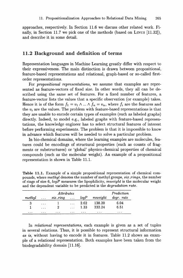
In bio-chemical domains, where the learning examples are molecules, features could be encodings of structural properties (such as counts of fragments or substructures) or 'global' physico-chemical properties of chemicalcompounds (such as the molecular weight). An example of a propositionalrepresentation is shown in Table 11.1.

Table 11.1. Example of a simple propositional representation of chemical compounds, where m ethyl denotes the number of methyl groups, six.rinqs , the numberof rings of size 6, logP measures the lipophilicity, mweight is the molecular weightand the dependent variable to be predicted is the degradation rate.

methyl

31

Attributessix_ring

12

logP

2.621.33

mweight

138.20232.24

Predictiondegr. rate

6.046.51

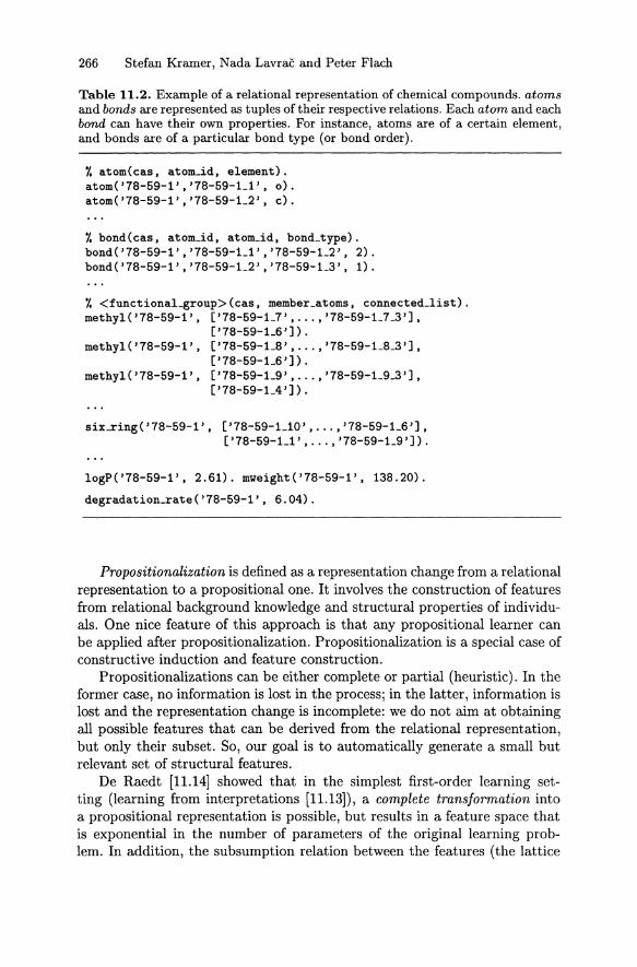
In relational representations, each example is given as a set of tuplesin several relations. Thus, it is possible to represent structural informationas is, without having to encode it in features . Table 11.2 shows an example of a relational representation. Both examples have been taken from th ebiodegradability domain [11.16].


Table 11.2. Example of a relational representation of chemical compounds. atomsand bonds are represented as tuples of their respective relations. Each atom and eachbond can have their own properties. For instance, atoms are of a certain element,and bonds are of a particular bond type (or bond order) .

%atom(cas. atom_id. element) .atom('78-59-1'.'78-59-1_1'. 0).atom('78-59-1'.'78-59-1_2', cl.

%bond(cas, atom_id. atom_id, bond_type).bond('78-59-1' ,'78-59-1_1' ,'78-59-1_2', 2).bond('78-59-1'.'78-59-1_2'.'78-59-1_3', 1).

% <functionaLgroup> (cas , membercatioms , connected.d.Lst ) .

methyl ('78-59-1'. ['78-59-L7' •.. .• , 78-59-L7-3'] •['78-59-L6']) .

methyl('78-59-1'. ['78-59-L8', ... , '78-59-L8_3'],['78-59-L6']) .

methyl( '78-59-1'. ['78-59-L9· •.. .• '78-59-L9-3'] •['78-59-L4']) .

six-ring(·78-59-1'. ['78-59-1_10' •.. .• '78-59-1_6'],['78-59-1_1', ...• '78-59-1_9']).

logP('78-59-1', 2.61). mweight('78-59-1', 138.20).

degradation_rate('78-59-1'. 6.04).

Propositionalization is defined as a representation change from a relationalrepresentation to a propositional one. It involves the construction of featuresfrom relational background knowledge and structural properties of individuals. One nice feature of this approach is that any propositional learner canbe applied after propositionalization. Propositionalization is a special case ofconstructive induction and feature construction.

Propositionalizations can be either complete or partial (heuristic) . In theformer case, no information is lost in the process ; in the latter, information islost and the representation change is incomplete: we do not aim at obtainingall possible features that can be derived from the relational representation,but only their subset. So, our goal is to automatically generate a small butrelevant set of structural features .

De Raedt [11.14] showed that in the simplest first-order learning setting (learning from interpretations [11.13]), a complete transformation intoa propositional representation is possible, but results in a feature space thatis exponential in the number of parameters of the original learning problem. In addition, the subsumption relation between the features (the lattice


of clauses) is no longer represented explicitly, so that it cannot be used orexploited in search in a straightforward manner.

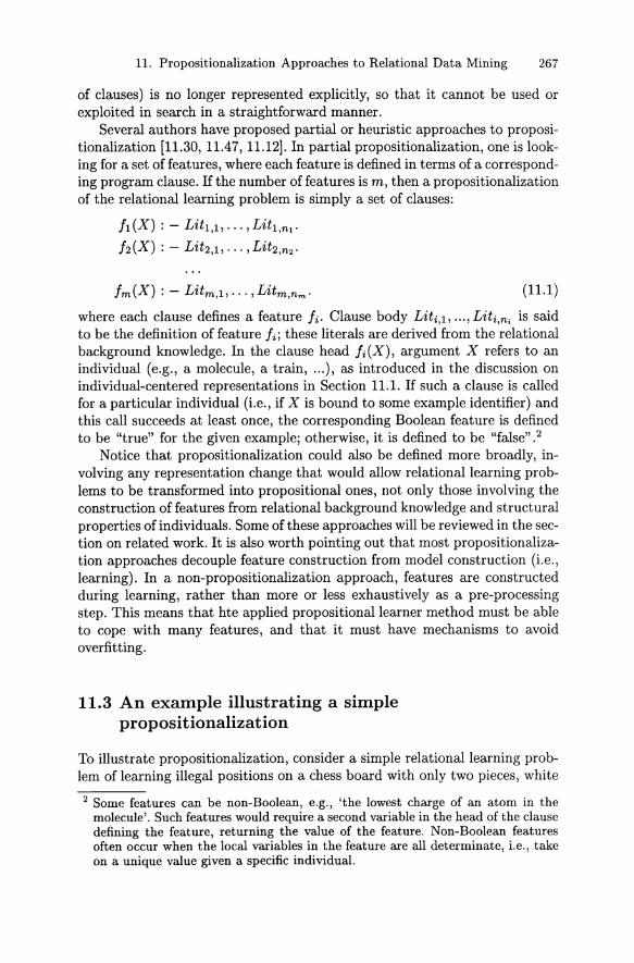
Several authors have proposed partial or heuristic approaches to propositionalization [11.30, 11.47, 11.12]. In partial propositionalization, one is looking for a set of features, where each feature is defined in terms of a corresponding program clause. If the number of features is m, then a propositionalizationof the relationallearning problem is simply a set of clauses:

!I (X) : - Litl ,l, .. . , Litl,nl'

h(X) : - Lit 2 ,1, . •. , Lih,n2'

fm(X) : - Litm,l, ... ,Litm,nm • (11.1)

where each clause defines a feature Ii. Clause body Liti,l, ... , Liti,ni is saidto be the definition offeature h: these literals are derived from the relationalbackground knowledge. In the clause head fi(X), argument X refers to anindividual (e.g., a molecule, a train, ...), as introduced in the discussion onindividual-centered representations in Section 11.1. If such a clause is calledfor a particular individual (i.e., if Xis bound to some example identifier) andthis call succeeds at least once, the corresponding Boolean feature is definedto be "true" for the given example; otherwise, it is defined to be "false" .2

Notice that propositionalization could also be defined more broadly, involving any representation change that would allow relationallearning problems to be transformed into propositional ones, not only those involving theconstruction of features from relational background knowledge and structuralproperties of individuals. Some of these approaches will be reviewed in the section on related work. It is also worth pointing out that most propositionalization approaches decouple feature construction from model construction (i.e.,learning). In a non-propositionalization approach, features are constructedduring learning, rather than more or less exhaustively as a pre-processingstep. This means that hte applied propositionallearner method must be ableto cope with many features, and that it must have mechanisms to avoidoverfitting.

11.3 An example illustrating a simplepropositionalization

To illustrate propositionalization, consider a simple relational learning problem of learning illegal positions on a chess board with only two pieces, white

2 Some features can be non-Boolean, e.g., 'the lowest charge of an atom in themolecule' . Such features would require a second variable in the head of the clausedefining the feature, returning the value of the feature. Non-Boolean featuresoften occur when the local variables in the feature are all determinate, i.e., takeon a unique value given a specific individual.

268 Stefan Kramer, Nada Lavrac and Peter Flach

king and black king. In this simplified example, a position P is a four-tuple P<WKf , WKr , BKf , BKr>, where WKf , WKr and BKf , BKr stand for the file and rankof white king and black king, respectively. Let illegal (WKf , WKr ,BKf , BKr)denote that the position in whieh the white king is at (WKf,WKr) and theblack king at (BKf, BKr) is illegal. Arguments WKf and BKf are of type file(with values a to h), while WKr and BKr are oftype rank (with values 1 to 8) .

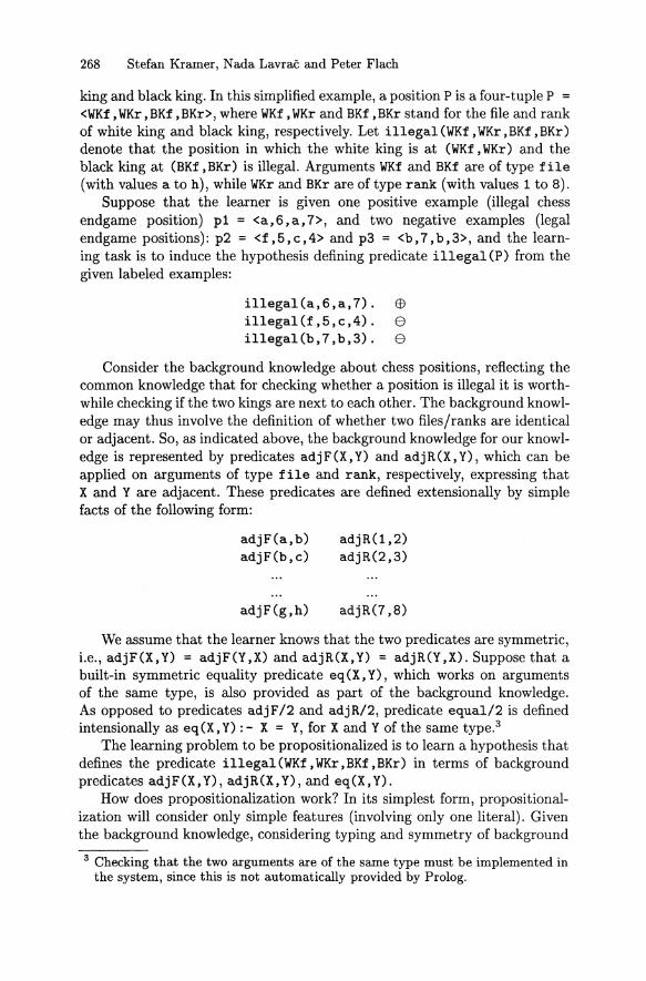
Suppose that the learner is given one positive example (illegal chessendgame position) p1 = <a,6,a,7> , and two negative examples (legalendgame positions): p2 = <f, 5 , c ,4> and p3 = <b, 7, b , 3> , and the learning task is to induce the hypothesis defining predieate illegal<P) from thegiven labeled examples:

illegal(a,6,a,7). ffiillegal(f,5,c,4). eillegal(b,7,b,3). e

Consider the background knowledge about chess positions, reflecting thecommon knowledge that for checking whether a position is illegal it is worthwhile checking if the two kings are next to each other. The background knowledge may thus involve the definition of whether two files/ranke are identiealor adjacent. So, as indieated above, the background knowledge for our knowledge is represented by predieates adj F(X, y) and adj R(X, Y), which can beapplied on arguments of type file and rank, respectively, expressing thatX and Y are adjacent. These predicates are defined extensionally by simplefacts of the following form:

adjF(a,b)adjF(b,c)

adjF(g,h)

adjR(1,2)adjR(2,3)

adjR(7,8)

We assurne that the learner knows that the two predicates are symmetric,i.e., adjF(X, Y) = adjF(Y,X) and adjR(X, Y) = adjR(Y ,X). Suppose that abuilt-in symmetrie equality predicate eq (X, Y), which works on argumentsof the same type, is also provided as part of the background knowledge.As opposed to predieates adjF/2 and adjR/2, predicate equal/2 is definedintensionally as eq (X, Y) : - X = Y, for X and Y of the same type.3

The learning problem to be propositionalized is to learn a hypothesis thatdefines the predicate illegal (WKf , WKr , BKf , BKr) in terms of backgroundpredieates adjF(X, Y), adjR(X, Y), and eq (X, Y).

How does propositionalization work? In its simplest form, propositionalization will consider only simple features (involving only one literai) . Giventhe background knowledge, considering typing and symmetry of background

3 Checking that the two arguments are of the same type must be implemented inthe system, since this is not automatically provided by Prolog.

11. Propositionalization Approaches to Relati onal Dat a Mining 269

predicates (allowing for only one of the two symmetric variants of a literal to be considered), only four simple features f i are taken int o account :eq(WKf,BKf) , eq(WKr,BKr) , adjF(WKf ,BKf) and adjR(WKr,BKr).

The given examples can now be transformed into four- tuples of the form:

(eq(WKf,BKf), eq(WKr,BKr), adjF(WKf,BKf) , adjR(WKr,BKr))

The actual propositional tuples are then constructed by evaluating thet ruth value of features for the given argument values of the ground factsof predicate illegal. More form ally if e E E is an example, and aJ is asubstitution such that illegal (P) aJ E E , the t ruth value of features isobtained by test ing whether fWj is t rue for the given background theoryB (haj is true if B 1= f iaj ). There are three such subst it utions, one foreach training example: a1 = P/<a,6,a,7>, a 2 = P/<f,5,c,4> and a3 =P/<b,7, b,3>.

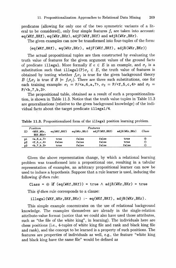
The propositional table, obtained as a resul t of such a propositionalization, is shown in Table 11.3. Notice that the truth value tuples in Table 11.3ar e generalizations (relat ive to the given background knowledge) of the individual facts about the target predicate illegal/4.

Table 11.3. P roposit ionalized form of t he illegal position learning problem .

Pos it ion Feat ure sID <IIKf .lIKr, eq(IIKf.B Kf) eq(lIKr ,BKr) adjF(IIKf,BKf) adjR (IIKr.BKr) Glass

BKf.BKr>

pl <a ,6 ,a,7> true false false true EBp2 <f.6.c.4> false false false true ep3 <b.7 .b.3> true fals e false false e

Given the ab ove representation change, by which a rela tional learningprobl em was t ransformed into a proposit ional one, resulting in a tabularrepresentation of examples, an arb it rary propositional learner can now beused to indu ce a hypothesis. Suppose that a ru le learner is used , inducing thefollowing if-then rul e:

Class = ffi if (eq(WKf,BKf)) = true A adjR(WKr,BKr) = true

This if-then rul e corresponds to a clause:

illegal(WKf,WKr,BKf,BKr) :- eq(WKf,BKf), adjR(WKr,BKr).

This simple example concent rates on the use of relation al backgroundknowledge. The examples themselves are already in the single-re lationattribute-value form at (notice that we could also have used those attributes,such as "t he file of the white king" , in learn ing). The individ uals here arechess positions (i.e., 4-tuples of white king file and rank and black king fileand rank), and the concept to be learned is a prop erty of such positions. Thefeatures are properties of ind ividuals as weIl, e.g., the feature "white kingand black king have the same file" would be defined as

270 Stefan Kramer , Nada Lavraö and Peter Flach

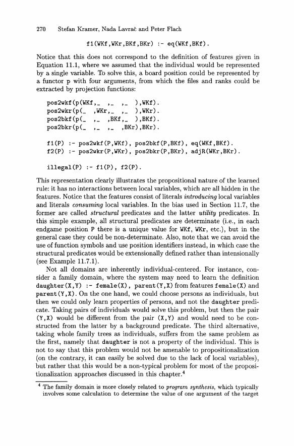
fl(WKf,WKr,BKf,BKr) :- eq(WKf,BKf) .

Notice that this does not correspond to the definition of features given inEquation 11.1, where we assumed that the individual would be representedby a single variable. To solve this, a board position could be represented bya functor p with four arguments, from which the files and ranks could beextracted by projection functions:

pos2wkf(p(WKf,_ ,_ ,_ ),WKf) .pos2wkr(p(_ ,WKr,_ ,_ ),WKr) .pos2bkf(p(_ ,_ ,BKf,_ ),BKf).pos2bkr(p(_ ,_ ,_ ,BKr),BKr).

f1(P)f2(P)

pos2wkf(P,WKf), pos2bkf(P,BKf), eq(WKf,BKf).pos2wkr(P,WKr), pos2bkr(P,BKr), adjR(WKr,BKr).

illegal(P) :- fl(P), f2(P) .

This representation clearly illustrates the propositional nature of th e learnedrule : it has no interactions between local variables, which are all hidden in thefeatures . Notice that the features consist of literals introduc ing local variablesand literals consuming local variables. In the bias used in Section 11.7, theformer are called structural predicates and the latter utility predicates. Inthis simple example, all structural predicates are determinate (i.e., in eachendgame position P there is a unique value for WKf, WKr, etc .) , but in thegeneral case they could be non-determinate. Also, note that we can avoid theuse of function symbols and use position identifiers instead, in which case thestructural predicates would be extensionally defined rather than intensionally(see Example 11.7.1).

Not all domains are inherently individual-centered. For instance, consider a family domain, where the system may need to learn the definitiondaughter(X, Y) : - female (X), parent (y ,X) from features female(X) andparent (y ,X). On the one hand, we could choose persons as individuals, butthen we could only learn properties of persons, and not the daughter predicate. Taking pairs of individuals would solve this problem, but then th e pair(Y ,X) would be different from the pair (X, Y) and would need to be constructed from the latter by a background predicate. The third alternative,taking whole family trees as individuals, suffers from the same problem asthe first, namely that daughter is not a property of the individual. This isnot to say that this problem would not be amenable to propositionalization(on the contrary, it can easily be solved due to the lack of local variables),but rather that this would be a non-typical problem for most of the propositionalization approaches discussed in this chapter.4

4 The family domain is more closely related to program synthesis, which typ icallyinvolves some calculation to determine the value of one argument of the target


Finally, the transformation shown in this section is an example of theLINUS system [11.32, 11.31] at work. In the following section, we will presentthis classical propositionalization system in some detail.

11.4 Feature construction for general-purposepropositionalization

This and the next section review some of the existing approaches to propositionalization. The review concentrates on the feature construction step. Wedistinguish between general-purpose approaches (this section) and specialpurpose approaches which are either domain-dependent , assurne a strongdeclarative bias, or are applicable to a limited problem class (Section 11.5).

11.4.1 LINUS

LINUS [11.32, 11.31] is a descendant ofthe learning algorithm used in QuMAS(Qualitative Model Acquisition System) which was used to learn functionsof components of a qualitative model of the heart in the KARDIO expertsystem for diagnosing cardiac arrhythmias [11.3]. The QuMAS learner andLINUS were the first systems to transform a relational representation into apropositional representation. The hypothesis language of LINUS is restrictedto function-free constrained DHDB (deductive hierarchical database) clauses .This implies that no recursion is allowed, and that no new variables may beintroduced. A clause is constrained if all variables in the body also occurin the head. An example of such a clause is daughter (X, Y) : - female (X) ,parent (Y , X). It should be clear that one can transform this kind of hypotheses into a propositional form, if female (X) and parent (Y, X) are defined asfeatures.

After propositionalization, users of the LINUS system can choose amonga number of propositional learning algorithms. These include the decisiontree induction system ASSISTANT [11.5], and two rule induction systems: anancestor of AQI5, named NEWGEM [11.37]' and CN2 [11.8, 11.7]. Recently,LINUS has been upgraded also with an interface to MLC++ [11.26]. Thehypotheses induced by either of these systems are translated back into firstorder logic to facilitate their interpretation.

DINUS [11.31] weakens the language bias of LINUS so that the system canlearn clauses with a restricted form of new variables, introduced by determinate literals. A literal is determinate if each of its variables that does notappear in preceding literals has only one possible binding given the bindings

predicate, given the others. It can be trivially transformed into a Boolean classification problem, by ignoring the input-output relations and viewing the programas a predicate rather than a function, but this ignores crucial information andmakes the task even harder.


of its variables that appear in preceding literals . An example of such clausesis:

grandmother(X,Y) : - father(Z,Y), mother(X,Z).grandmother(X,Y) : - mother(U,Y), mother(X,U) .

Th is restriction allows for a similar transformation approach as the one takenin LINUS.

11.4.2 Stochastic propositionalization

Kramer et al. [11.30) developed a method that finds sets offeatures that together possess good discriminatory power. Stochastic search is used to findclauses of arbitrary length, where each clause corresponds to a binary feature.The search strategy employed is similar to random mutation hill-climbing.Over a predefined number of episodes, the algorithm develops a set of mclauses. An elementary step in this search consists of the replacement of anumber of clauses in the current generation. The removal of clauses as wellthe addition of new ones is done probabilistically, i.e., with a prob abilityproportional to the fitness of individual clauses. The fitness function of individual clauses/features is based on the Minimum Description Length (MDL)principle. Also, we impose constraints on desirable features , for inst ance, ontheir generality and specificity. For the final selection of one generation offeatures, we evaluate sets of features/clauses by the resubstitution est imate(i.e., the training set error) of the decision table constructed from all featuresin the set .

An example for a feature found by this method is:

fl(A) :- atm(A, B, _, 27, _),bond(A, B, C, _),atm(A, C, _,29, _) .

This feature is "t rue" if in compound A there exists a bond between an atomof type 27 (according to the biomolecular modeling package QUANTA) andan atom of type 29. While this is still a relatively simple feature, in somedomains the average length was about 4 and the standard deviation was up to3. So, the method often is able to search deeper than other methods due to itsflexible "search horizon" , but cannot provide guarantees for the optim ality orcompleteness of its propositionalizations. This method also differs from othermethods in that it works in a class-sensitive manner and th at it at temptsto find features that work well together (not just features that are usefulindividually) .

11.4.3 PROGOL

Srinivasan and King [11.47) presented a method for feature construction basedon hypotheses returned by PROGOL [11.38) . For each clause, each input-


output connected subset of literals is used to define a feature. For instance,if PROGOL returns a theory

inaetive(A) ;- has_rings(A, [Rl, R2]),hydrophobie(A, H),H > 1.0.

then this approach would come up with the following feature definitions:

fl(A) has_rings(A, [Rl, R2]) .f2(A) hydrophobie(A, H) .f3(A) hydrophobie(A, H), H > 1.0 .f4(A) has_rings(A, [Rl, R2]), hydrophobie(A, H) .f5(A) has_rings(A, [Rl, R2]), hydrophobie(A, H), H > 1.0 .

Since f2 would be true for all examples, the system would discard it in asubsequent step. The authors used these "ILP-features" in multiple linearregression.

This method works for all types of background knowledge. Besides, itcould be applied to any ILP algorithm.

11.4.4 WARMR

WARMR [11.12] is an algorithm for finding association rules over multiplerelations. The main step of the algorithm consists of detecting frequentlysucceeding Datalog queries . Queries returned by WARMR have been successfully used to construct features from relational background knowledge.

Datalog is a Prolog-like language used for deductive databases that excludes function symbols . A Datalog query is an expression of the form? - Al , . .. , An, where Al " ", An are logical atoms. Such a query denotesa conjunction of conditions. The WARMR system automatically generatesqueries up to a certain length, and returns thos e t hat succeed for a sufficientnumber of cases. A query is frequently succeeding, if the conditions in it holdfor a sufficient number of examples in the dataset.

Given a representation in Datalog, this approach can be applied to theproblem of detecting commonly occurring substructures in chemical compounds. One simply asks for frequently succeeding queries, where Al , . . . , Andenote structural properties of compounds. An example for such a query is

? - six_ring(C, S) ,atomel(C, Al, h), atomel(C, A2 , c), bond(C, Al, A2 , X) .

If such a query is known to succeed for a sufficient number examples C, it isturned into a feature:

fl(C) :- six_ring(C,S), atomel(C,Al, h),atomel(C,A2,e) , bond(C,Al,A2,X) .

WARMR features have been used with several propositional learning algorithms, e.g. , C4 .5[11.44].


11.5 Special-purpose feature construction

In this section, we review some of the existing approaches to propositionalization that proved to be successful in solving specific learning tasks, eitherdue to assuming a very strong language bias (graph-based approaches) ordue to being designed only for very specialized tasks. Despite their specificity, reviewing of these approaches may serve the reader as a source of ideasfor designing special-purpose feature construction methods for new learningproblems to be solved.

11.5.1 Turney's approach applied in the East-West challenge

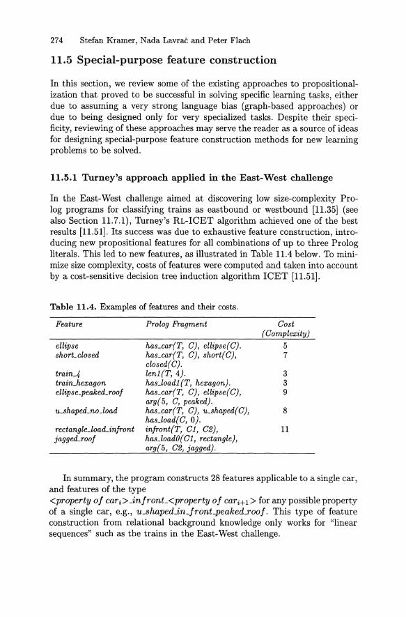
In the East-West challenge aimed at discovering low size-complexity Prolog programs for classifying trains as eastbound or westbound [11.35] (seealso Section 11.7.1), Turney's RL-ICET algorithm achieved one of the bestresults [11.51]. Its success was due to exhaustive feature construction, introducing new propositional features for all combinations of up to three Prologliterals. This led to new features, as illustrated in Table 11.4 below. To minimize size complexity, costs of features were computed and taken into accountby a cost-sensitive decision tree induction algorithm ICET [11.51] .

Table 11.4. Examples of features and their costs.

Feature

ellipseshorL closed

train_4train.hexaqor:ellipse.peoked.roo]

rectcnqle.load.imjrotüjagged_roof

Prolog Fragment

has_car{T, C) , ellipse{C).has_car{T, C) , short{C),closed{C).lenl{T,4).has.loadl (T, hexagon).has.cort'I', C) , ellipse{C),arg{5, C, peaked) .has.cart'I', C) , u_shaped{C),has.loadtO, 0).infront{T, Cl, C2) ,has_loadO{Cl, rectangle),arg{5 , C2, jagged) .

Cost(Complexity)

57

339

8

11

In summary, the program constructs 28 features applic able to a single car ,and features of the type<property 0/ cari>_in/ronL<property 0/ cari+l> for any possible propertyof a single car, e.g., u.shaped.in.front.peaked.roo] , This type of featureconstruction from relational background knowledge only works for "linearsequences" such as the trains in the East-West challenge.


11.5.2 Cohen's set-valued features

Cohen [11.10] introduced the notion of "set-valued features" , which can beused to transform certain types of background knowledge. A value of a setvalued feature is allowed to be a set of strings. This type of feature caneasily be incorporated in existing propositional learning algorithms. Somefirst-order learning problems (e.g., text categorization) can be propositionalized in this way.

11.5.3 Geibel and Wysotzki's graph-based approach

Geibel and Wysotzki [11.22] proposed a method for feature constructionin a graph-based representation. The features are obtained through fixedlength paths in the neighborhood of anode in the graph. This approachdistinguishes between "context-dependent node attributes of depth n" and"context-dependent edge attributes of depth n". A context-dependent nodeattribute An(G)[i,i] is defined as follows. For each node i in graph G, wedefine the context of i (of depth n) as all length n paths from node i and tonode i. Each such context is used to define a feature. The feature value foran example graph is the number of occurrences of the corresponding contextin it . Analogously, a context-dependent edge attribute An(G)[i, j] is definedin terms of alllength n paths from node i to node j in graph G.

11.5.4 SUBDUE

SUBDUE [11.11] is an MDL-based algorithm for substructure discovery ingraphs. SUBDUE finds substructures that compress th e original data and represent structural concepts in the data. After SUBDUE has identified a compressive substructure, it replaces all occurrences in the graph and continuessearch in the transformed graph. In multiple passes of this kind, SUBDUEproduces a hierarchical description of the structural regularities in the data.It has to be emphasized that SUBDUE is capable of identifying subgraphs,not just linearly connected fragments.

11.5.5 CASEjMuLTICASE

The CASE/MuLTICASE syst ems [11.23, 11.24] represent remarkable propositionalization approaches in the computational chemistry literature.

The development of a CASE [11.23] model starts with a training set , containing chemical structures and biological activities. Each molecule is splitinto all possible linear subunits with two to ten non-hydrogen atoms (the sizeof fragment varies in CASE related publications) . All fragments belongingto an active molecule are labeled active, while those belonging to an inactive molecule are labeled inactive. To identify relevant substructures, CASE


assurnes a binomial distribution and takes a statistically significant deviation from random distribution as indication that the fragment is relevantfor biological activity. In the prediction step, the probability of activity isestimated using Bayesian statistics based on the presence of the significantfragments. MULTICASE differs from CASE in that it employs separate-andconquer (as in rule induction) to select one relevant fragment after the other.CASE/MuLTICASE is quite similar to the approach described in the following section. However, since no technical details are known about fragmentgeneration in CASE/MuLTICASE, it is hard to determine the similarities anddifferences between these approaches.

11.5.6 Kramer and Frank's propositionalization methods forgraph-based domains

Kramer and Frank [11.29] present a method for propositionalization that istailored for domains, where the examples are given as labeled graphs. Themethod is designed to discover all linearly connected vertices of some type(i.e., labeled in some way) that occur frequently in the examples (up to someuser-specified length).

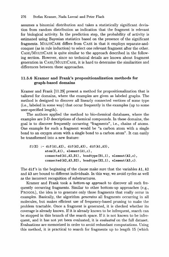
The authors applied the method to bio-chemical databases, where theexamples are 2-D descriptions of chemical compounds. In these domains, thegoal is to discover frequently occurring "fragments", i.e., chains of atoms.One example for such a fragment would be "a carbon atom with a singlebond to an oxygen atom with a single bond to a carbon atom". It can easilybe transformed into a new feature:

f1(X) :- dif(A1,A2), dif(A2,A3), dif(A1,A3),atom(X,A1), element(A1,c),connected(A1,A2,B1), bondtype(B1,1) , element (A2,o),connected(A2,A3,B2), bondtype(B2, 1) , element(A3,c) .

The dif's in the beginning of the clause make sure that the variables Al , A2and A3 are bound to different individuals. In this way, we avoid cycles as weIlas the incorrect recognition of substructures.

Kramer and Frank took a bottom-up approach to discover all such frequently occurring fragments. Similar to other bottom-up approaches (e.g.,PROGOL), the idea is to generate only those fragments that really occur inexamples. BasicaIly, the algorithm generates all fragments occurring in allmolecules, but makes efficient use of frequency-based pruning to make theproblem tractable. Once a fragment is generated, it is checked whether itscoverage is already known. If it is already known to be infrequent, search canbe stopped in this branch of the search space. If it is not known to be infrequent, and it has not yet been evaluated, it is evaluated on the full dataset .Evaluations are memorized in order to avoid redundant computations. Usingthis method, it is practical to search for fragments up to length 15 (which


takes a few hours computation time on a Linux PC with a Pentium II processor).

After propositionalization, an algorithm for support vector machines[11.52, 11.53, 11.4] is applied to the transformed problem. Support vectormachines seem particularly useful in the context of propositionalization, asthey can deal with a large number of moderately significant features.

Preliminary experiments in the domain of carcinogenicity predictionshowed that bottom-up propositionalization is a promising approach to feature construction from relational data: frequent fragments are found in areasonable time and the predictive accuracy obtained using these fragmentsis very good.

11.6 Related transformation approaches

In its broadest sense, the related work involves various different approachesto constructive induction [11.43, 11.54, 11.42, 11.27] and predicate invention(some of which are presented in an overview paper by Stahl [11.50]).

More closely related are transformation approaches, usually restricted tosome particular form of background knowledge, which do not necessarily result in a table where one row corresponds to a single example. Some of theseresult in a table with multiple rows corresponding to a single training example; these representations are known as multiple-instance learning problems[11.15].

11.6.1 Zucker and Ganascia's transformation approach

Zucker and Ganascia [11.56, 11.57] proposed to decompose structured examples into several learning examples, which are descriptions of parts of whatthey call the "natural example". The transformation results in a table withmultiple rows corresponding to a single example. For instance, any combination of two cars of a train would be defined to be an example. Note that aproblem which is reformulated in this way is not equivalent to the originalproblem. Although it is not clear whether this approach could successfullybe applied to, e.g., arbitrary graph structures, their system REMO solves theproblem of learning structurally indeterminate clauses, much in line withthe extended LINUS propositionalization approach presented in Section 11.7.Their definition of structural clauses whose bodies contain exclusively structural literals, and their algorithm for learning structurally indeterminateclauses can be seen as one of the predecessors of the extended LINUS approach. Recent work by Chevaleyre and Zucker [11.6] further elaborates onthe issue of transformed representations for multiple-instance data.


11.6.2 Transformation approach by Fensel et al.

Fensel et al. [11.17] achieve the transformation from the first-order repre sentation to the propositional representation by ground substitutions over agiven, user-defined alphabet which transform clauses to ground clauses. As aconsequence, they introduce a new definition of positive and negative examples: instead of ground facts they regard ground substitutions as examples.For every possible ground substitution (depending on the number of variablesand the alphabet), there is one example in the transformed problem representation. Each background predicate, together with the variable it uses, definesa binary attribute. Like in the previous approach, an example is not describedby a single row in the resulting table, but by several rows.

11.6.3 STILL

STILL [11.46] is an algorithm that performs "stochastic matching" in thetest whether a hypothesis covers an example. It operates in the so-calledDisjunctive Version Space framework, where for each positive example E,one is interested in the space of all hypotheses covering E and excluding allnegative examples Fi •

In order to transfer the idea of disjunctive version spaces to first-orderlogic, STILL reformulates first-order examples in a propositional form. Likein the work by Fensel et al., substitutions are handled as attribute-value examples. In contrast to LINUS and REMO, this reformulation is bottom-uprather than top-down. It is not performed for the complete dataset, but onlyfor one seed example E and for counter-examples Fi . The reformulation isone-to-one (one example, one row) for the seed example, and one-to-many(one example, several rows) for the counter-examples. Since it would be intractable to use all possible substitutions for the counter examples, STILLstochastically samples a subset of these. STILL uses a representation whicheffectively yields black-box classifiers instead of intelligible features .

11.6.4 PROPAL

PROPAL [11.2] is arecent propositionalization approach which does notpropositionalize according to a fixed set of features, but rather extends eachhypothesis (Boolean vector) when it is found to be overly general (covering anegative example). PROPAL works in function-free, non-recursive Horn logic.A seed example is chosen and maximally variabilized, serving as the pattern against which other examples are propositionalized. The pattern consistsboth of non-ground literals and the equality constraints which hold betweenvariables in the seed example. The actual learning algorithm is an AQ-likealgorithm.


11.7 A sample propositionalization method: ExtendingLINUS to handle non-determinate literals

In this section, we show that LINUS can be extended to learning ofnon-determinate clauses, provided that the problem domain is individualcentered. The approach can not be extended to program synthesis or taskswhich do not have a clear notion of an individual. To illustrate this propositionalization approach, we first present a running example that will be usedthroughout the remainder of the section.

11.7.1 The East-West challenge example

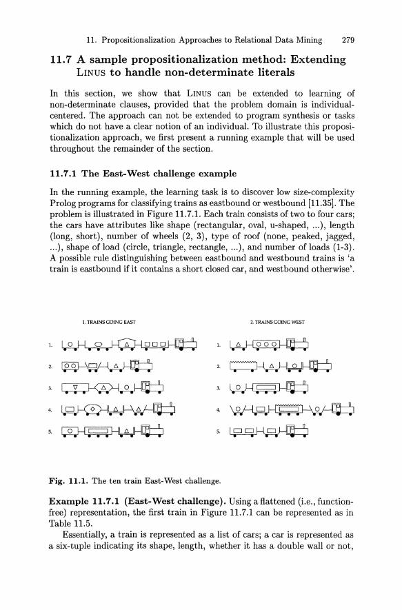
In the running example, the learning task is to discover low size-complexityProlog programs for classifying trains as eastbound or westbound [11.35]. Theproblem is illustrated in Figure 11.7.1. Each train consists oftwo to four cars;the cars have attributes like shape (rectangular, oval, u-shaped, ...), length(long, short), number of wheels (2, 3), type of roof (none, peaked, jagged,...), shape of load (circle, triangle, rectangle, ...), and number of loads (1-3).A possible rule distinguishing between eastbound and westbound trains is 'atrain is eastbound if it contains a short closed car, and westbound otherwise' .

\. TRAINSGOING EAST 2. TRAINSGOING WEST

\. I.~

2.~

3.~

4. 4.

S.~ 5.~

Fig. 11.1. The ten train East-West challenge.

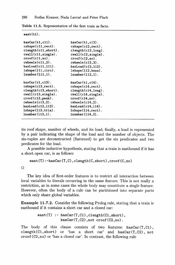
Example 11.7.1 (East-West challenge). Using a flattened (l.e., functionfree) representation, the first train in Figure 11.7.1 can be represented as inTable 11.5.

Essentially, a train is represented as a list of cars; a car is represented asa six-tuple indicating its shape, length, whether it has a double wall or not,

280 Stefan Kr amer , Nada Lavraö and Peter Flach

Table 11.5. Represent ati on of the first t rain as fact s.

east(t!) .

hasCar(t1,e11) .eshape(e11,reet).elength(e11,short).evall(e11,single).eroofCe11,no) .evheels (e11, 2) .hasLoad(e11,111) .lshape(111,eire).Inumber (111,1) .

hasCar (ti,c13) .eshape(e13,reet) .elength(e13,short).evall(e13 ,single) .eroof(c13,peak) .evheels(e13,2).hasLoad(e13,113) .lshape(113,tria).Inumber(113,1).

hasCar(ti,e12).eshape(e12,reet).elength(e12.1ong) .evall(e12,single).eroofCe12 ,no) .evheels(e12.3).hasLoad(e12 .112) .lshape(112,hexa) .InumberC112.!) .

hasCar(t1,e14).eshape(e14 .reet) .elength(e14,long) .evall(e14,single) .eroof(c14,no).evheels(e14,2) .hasLoad(e14,114).lshape(114,reet) .Inumber(114,3) .

its roof shape, number of wheels, and its load ; finally, a load is representedby a pair indicating the shape of the load and the number of objects. Thesix-tuples are deeonst ru eted (ßattened) to get the six predieates and twopredieates for the load.

A possible inductive hypothesis, stating that a t ra in is eastbound if it hasa short open ear, is as follows:

east(T) ;-hasCar(T,C),clength(C,short),croof(C,no)

o

The key idea of first-order features is to restriet all interaction betweenloeal variables to literals oeeurring in the same feature. This is not really arest rict ion, as in some eases the whole bod y may eonstitute a single feature.However , ofte n the body of a rule ean be partitioned into separate partswhich only share global vari ables.

Example 11.7.2. Consider the following P rolog rule, stating that a train iseastbound if it eont ains a short ear and a closed ear:

east(T) ; - hasCar(T ,Cl),clength(Cl,short),hasCar(T ,C2),not croof(C2 ,no) .

The body of this clause eonsists of two featur es: hasCar (T , Cl) ,clength(Cl,short) or 'has a short ear ' and hasCar (T,C2), notcroof(C2 ,no) or 'has a closed ear' . In eontrast , the following rule


east(T):-hasCar(T,C),clength(C,short) ,not croof(C,no)

contains a single feature expressing the property 'has a short closed car '.o

11.7.2 The extended LINUS propositionalization approach:Propositionalization through first-order featureconstruction

In this section, we propose a general-purpose propositionalization method,complete with respect to a given language bias, provided that the problemunder consideration can be represented in an individual-centered representation. We start by providing a declarative bias for first-order feature construction, and continue by giving an experimental evaluation of the proposedapproach.

The declarative feature bias is based on the term-based individualcentered representations introduced by Flach et al. [11.19] and further developed by Flach and Lachiche [11.20]. Such representations collect all information about one individual in a single term, e.g., a list of 6-tuples. Rulesare formed by stating conditions on the whole term, e.g., length (T, 4), orby referring to one or more subterms and stating conditions on those subterms. Predicates which refer to subterms are called structural predicates:they come with the type of the term, e.g., list membership comes with lists,projections (n different ones) come with n-tuples, etc. Notice that projections are determinate, while list membership is not . In fact, the only placewhere non-determinacy can occur in individual-centered representations is instructural predicates.

Individual-centered representations can also occur in flattened form. Inthis case each of the individuals and most of its parts are named by constants,as in Example 11.7.1. It is still helpful to think of the flattened representation to be obtained from the term-based representation. Thus, hasCar corresponds to lisr/set membership and is non-determinate (i.e., one-to-many),while hasLoad corresponds to projection onto the sixth component of a tuple and thus is determinate (Le., one-to-one) . Keeping this correspondencein mind, the following definitions for the non-flattened case can be easilytranslated to the flattened case.

We assurne a given type structure defining the type of the individual. Let T

be a given type signature, defining a single top-level type in terms of subtypes.A structural predicate is a binary predicate associated with a complex typein T representing the mapping between that type and one of its subtypes.A functional structural predicate, or structural function, maps to a uniquesubterm, while a non-determinate structural predicate is non-functional."

5 In other words, the predicate maps to sets of terms, i.e., it does not return aunique value .


In general, we have a structural predicate or function associated with eachnon-atomic subtype in T. In addition, we have utility predicates as in LINUS

[11.32, 11.31] (calIed properties by Flach and Lachiche [11.20]) associatedwith each atomic subtype, and possibly also with non-atomic subtypes andwith the top-level type (e.g., the dass predicate). Utility predicates differfrom structural predicates in that they do not introduce new variables.

Example 11.7.3. For the East-West challenge we use the following type signature. train is declared as the top-level set type representing an individual.The structural predicate hasCar non-deterministically selects a car from atrain. car is defined as a 6-tuple. The first 5 components of each 6-tuple areatomic values, while the last component is a 2-tuple representing the load,selected by the structural function hasLoad. In addition, the type signaturedefines the following utility predicates (properties): east is a property of thetop-level type train, the following utility predicates are used on the subtype car: cshape, clength, cwall, croof and cwheels, whereas lshape andlnumber are properties of the sub-subtype load.o

To summarize, structural predicates refer to parts of individuals (theseare binary predicates representing a link between a complex type and one ofits components; they are used to introduce new local variables into rules),whereas utility predicates present properties of individuals or their parts, represented by variables introduced so far (they do not introduce new variables) .The language bias expressed by mode declarations used in other ILP learnerssuch as PROGOL [11.38] or WARMR [11.12]) partly achieves the same goal byindicating which of the predicate arguments are input (denoting a variable already occurring in the hypothesis currently being constructed) and which areoutput arguments, possibly introducing a new local variable. However, modedeclarations constitute a bias for the body rather than a bias for features.

Declarations of types, structural predicates and utility predicates definethe bias for features . The actual first-order feature construction will be restricted by parameters that define the maximum number of literals constituting a feature , maximal number of variables, and the number of occurrencesof individual predicates.

A first-order feature can now be defined as folIows. A first-order featureof an individual is constructed as a conjunction of structural predicates andutility predi cates which is well-typed according to T. Furthermore:

1. there is exactly one individual variable with type T, which is free (i.e.,not quantified) and will play the role of the global variable in rules;

2. each structural predicate introduces a new existentially quantified localvariable, and uses either the global variable or one of the local variablesintroduced by other structural predicates;

3. utility predicates do not introduce new variables (this typically meansthat one of their arguments is requ ired to be instantiated);


4. all variables are used either by a structural predicate or a utility predicate.

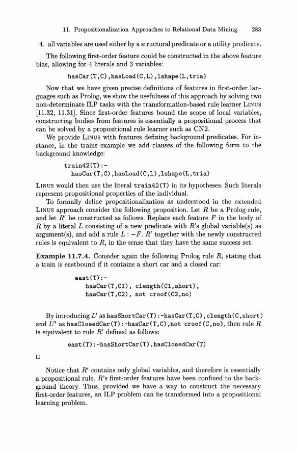
The following first-order feature could be constructed in the above featurebias, allowing for 4 literals and 3 variables:

hasCar(T,C),hasLoad(C,L),lshape(L,tria)

Now that we have given precise definitions of features in first-order languages such as Prolog, we show the usefulness of this approach by solving twonon-determinate ILP tasks with the transformation-based rule learner LINUS[11.32, 11.31). Since first-order features bound the scope of local variables,constructing bodies from features is essentially a propositional proces s thatcan be solved by a propositional rule learner such as CN2.

We provide LINUS with features defining background predicates. For instance, in the trains example we add clauses of the following form to thebackground knowledge:

train42(T):-hasCar(T,C) ,hasLoad(C,L) ,1shape(L,tria)

LINUS would then use the literal train42 (T) in its hypotheses. Such literalsrepresent propositional properties of the individual.

To formally define propositionalization as understood in the extendedLINUS approach consider the following proposition. Let R be a Prolog rule ,and let R' be constructed as folIows. Replace each feature F in the body ofR by a literal L consisting of a new predicate with R's global variable(s) asargument(s) , and add a rule L : -F. R' together with the newly constructedrules is equivalent to R, in the sense that they have the same success set .

Example 11.7.4. Consider again the following Prolog rule R, stating thata train is eastbound if it contains a short car and a closed car:

east(T):-hasCar(T,Cl), clength(Cl,short),hasCar(T,C2), not croof(C2,no)

By introducing L' as hasShortCar(T) : -hasCar(T ,C) ,clength(C, short)and L" as hasClosedCar (T) : -hasCar (T ,C) ,not croof (C, no) , then rule Ris equivalent to rule R' defined as follows:

east(T):-hasShortCar(T) ,hasClosedCar(T)

o

Notice that R' contains only global variables, and therefore is essent iallya propositional rule. R's first-order features have been confined to the background theory. Thus, provided we have a way to construct the necessaryfirst-order features, an ILP problem can be transformed into a propositionallearning problem.


11.7.3 Experimental results

In the two experiments reporte d in thi s section we simply provide LINUS

with all features that can be generated within a given feature bias (reca llthat such a feature bias includes bounds on the number of lit erals and firstorder features).

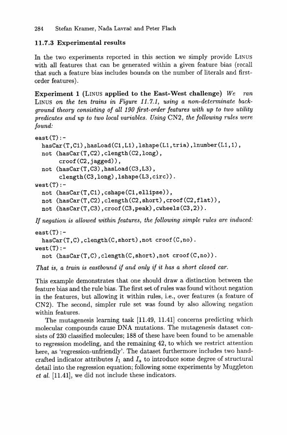
Experiment 1 (LINUS applied to the East-West challenge) We ttui

L INUS on the ten trains in Figure 11.7.1, using a non-determinate background theory consisting of all 190 first-o rder features with up to two utilitypredicates and up to two local variables. Using CN2, the follow ing rules werefound:

east(T) :-hasCar(T,C1),hasLoad(C1,L1),lshape(L1,tria),lnumber(L1,1),not (hasCar(T,C2),clength(C2,long),

croof(C2,jagged»,not (hasCar(T,C3),hasLoad(C3,L3),

clength(C3,long),lshape(L3,circ».west(T):-

not (hasCar(T,C1),cshape(C1,ellipse» ,not (hasCar(T,C2),clength(C2,short),croof(C2,flat»,not (hasCar(T,C3),croof(C3,peak),cwheels(C3 ,2».

I] negation is allowed within features, the following simple rules are in duced:

east(T):-hasCar(T,C),clength(C,short),not croof(C,no) .

west(T): -not (hasCar(T,C) ,clength(C,short),not croof(C,no».

That is, a train is easibound if and only if it has a short closed car.

This example demonstrates that one should draw a dist inction between thefeature bias and the ru le bias. The first set of rules was found without negationin the features, but allowing it within rules, i.e., over features (a feature ofCN2). Th e second, simpler rule set was found by also allowing negationwithin features.

Th e mutagenesis learning task [11.49, 11.41] concerns predictin g whichmolecular compounds cause DNA mutations. The mutagenesis dataset consists of 230 classified molecules; 188 of these have been found to be amenab leto regression modeling, and the remaining 42, to which we rest riet attent ionhere, as 'regression-unfriendly' . The dataset furthermore includes two handcrafted indicator attributes li and l a to introduce some degree of st ructuraldetail into the regression equation; following some experiments by Muggletonet al. [11.41], we did not include these indicators.


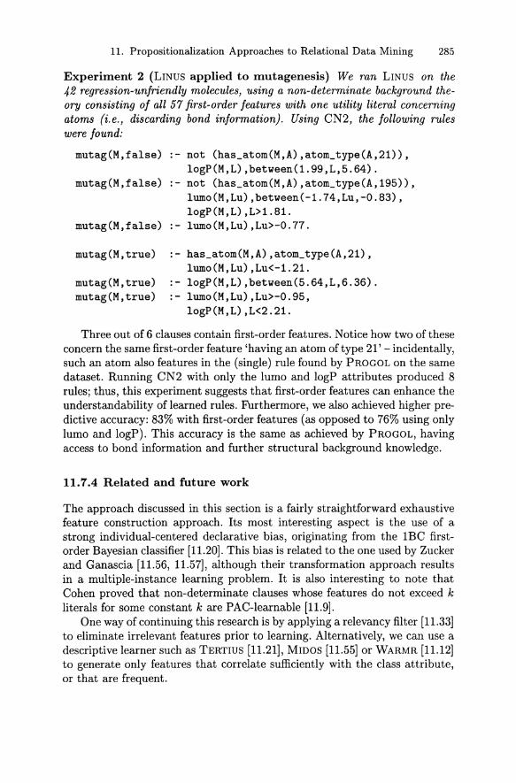
Experiment 2 (LINUS applied to mutagenesis) We ran LINUS on the42 regression-unjriendly molecules, using a non-determinate background theory consisting of all 57 first-order features with one utility literal concerningatoms (i.e., discarding bond information). Using CN2, the following ruleswere found:

mutag(M,false)

mutag(M,false)

mutag(M,false)

mutag(M,true)

mutag(M,true)mutag(M,true)

not (has_atom(M,A),atom_type(A,21)),logP(M,L),between(1.99,L,5.64).

' - not (has_atom(M,A),atom_type(A,195)),lumo(M,Lu),between(-1.74,Lu,-O.83),logP(M,L),L>1.81.lumo(M,Lu),Lu>-O.77.

has_atom(M,A) ,atom_type(A,21),lumo(M,Lu),Lu<-1.21.logP(M,L),between(5.64,L,6 .36).lumo(M,Lu),Lu>-O.95,logP(M,L),L<2.21.

Three out of 6 clauses contain first-order features. Notice how two of theseconcern the same first-order feature 'having an atom of type 21' - incidentally,such an atom also features in the (single) rule found by PROGOL on the samedataset. Running CN2 with only the lumo and logP attributes produced 8rules; thus, this experiment suggests that first-order features can enhance theunderstandability of learned rules. Furthermore, we also achieved higher predictive accuracy: 83% with first-order features (as opposed to 76% using onlylumo and logP) . This accuracy is the same as achieved by PROGOL, havingaccess to bond information and furt her structural background knowledge.

11.7.4 Related and future work

The approach discussed in this section is a fairly straightforward exhaustivefeature construction approach. Its most interesting aspect is the use of astrong individual-centered declarative bias, originating from the IBC firstorder Bayesian classifier [11.20]. This bias is related to the one used by Zuckerand Ganascia [11.56, 11.57], although their transformation approach resultsin a multiple-instance learning problem. It is also interesting to note thatCohen proved that non-determinate clauses whose features do not exceed kliterals for some constant kare PAC-Iearnable [11.9].

One way of continuing this research is by applying a relevancy filter [11.33]to eliminate irrelevant features prior to learning. Alternatively, we can use adescriptive learner such as TERTIUS [11.21], MIDOS [11.55] or WARMR [11.12]to generate only features that correlate sufficiently with the class attribute,or that are frequent.


11.8 Concluding remarks

In this chapter, we gave an overview of work in propositionalization, andpresented one of the methods in detail. To summarize the scope of the chapter:

- We focused on induction in the learning from interpretations framework[11.14] . This means, we restricted ourselves to cases where an "ordinary"relational database is given for learning. Thus, we exclude all settings forlearning in first-order logic that are more complicated (e.g., dealing withstructured terms and recursion).

- De Raedt [11.14] showed that for the above mentioned learning setting,complete propositionalizations are possible, but result in learning problems that are, in size, exponential in a number of parameters of the originallearning problem. This chapter presented work on heuristic, partial propositionalizations, which generate only a subset of the features derivable fromthe relational background knowledge within a given language bias .

- The work presented here focusses on individual-centered representations,i.e., representations that build upon the notion of individuals (here, described in terms of relations). For the given set of individuals, we compute arelatively smaIl, but relevant (sub- )set of structural properties. This type ofrepresentation excludes applications such as program synthesis and learn ing of relations between/among individuals. (Note that this restriction isrelated to the first point in this list) .

- All approaches described in this chapter have in common that they onlyconstruct features described in terms of conjunctions of literals. It wouldbe conceivable to construct disjunctive features as weIl, but obviously thesearch space would be vast .

In this chapter, we have seen general-purpose propositionalization methods as weIl as special-purpose ones. While the first group of methods is readilyavailable and applicable, it cannot exploit characteristics of the applicationdomains to improve efficiency. Clearly, the advantages and disadvantages ofthese two groups of methods are complementary.

The work described in this chapter is also related to applications whereILP is used to handle learning examples that are not handled successfullyby propositional systems. For instance, the original paper on the weIl-knownmutagenicity application [11.49] shows that PROGOL performs weIl on th e setof 42 regression-unfriendly examples, i.e., those examples, that are not weIlhandled by stepwise multiple linear regression. Another work in this directionwas the submission made by Srinivasan et al. to the PTE-2 challenge [11.48],where errors made by C4.5 on the training set were corrected by PROGOL.

The combined model turned out to be optimal under certain misclassification costs and/or class distributions according to ROC curve analysis. Aninteresting direction of further work would be to use fuIl-fiedged relationallearning to correct errors made by a propositionallearner applied to a propositionalization.


It should be stressed that feature construction can play an important rolewith respect to the reusability of constructed features . Individual problemareas have particular characteristics and requirements, and researchers aimat developing specialized learners for such applications. This may involve alsothe development of libraries, background knowledge and previously learnedhypotheses to be stored for further learning in selected problem areas. In thecontext of this chapter, we wish to emphasize that feature construction mayresult in components that are worth to be stored in background knowledgelibraries and reused for similar types of applications. Notice that such librariesare now being established for selected problem areas in molecular biology. Oneshould be aware, however, that an increased volume of background knowledgemay have also undesirable properties: not only that learning will become lessefficient, but with possibly irrelevant information being stored in backgroundknowledge libraries, results of learning will be less accurate. Therefore it iscrucial to employ criteria for evaluating the relevance of constructed featuresbefore they are allowed to become part of a library of background knowledgefor a specific application area. Work in irrelevant feature elimination mayhelp to filter out features irrelevant for the task at hand [11.33].

Propositionalizations have been shown to work successfully in a number ofdomains. However, it has to be emphasized that this is no argument againstILP, because ILP-type techniques are required for propositionalizations asweIl. Work on propositionalization has to be considered as apart of ILP research. (ActuaIly, it was there quite early on [11.32, 11.31].) While learningdirectly in relational representations is still an open research topic (despite recent successes), learning with propositionalizations is a practical option withthe nice property that progress in propositionallearning can immediately beutilized (see, e.g., the recent work by one of the authors applying SupportVector Machines [11.52, 11.53, 11.4] after propositionalization).

Acknowledgments

We are grateful to Marko Grobelnik and Saso Dzeroski for joint work onLINUS, and Nicolas Lachiche for the joint work on individual-centered representation resulting and implementing feature generation within the IBCsystem which we used for the extended LINUS propositionalization method.This work has been supported by the Slovenian Ministry of Science andTechnology, the EU-funded project Data Mining and Decision Support forBusiness Competitiveness: A European Virtual Enterprise (IST-1999-11495),and the British Council (ALlS link 69).

References

11.1 R . Agrawal, H. Mannila, R. Srikant, H. Toivonen, and A.I. Verkamo. Fastdiscovery of association rules. In U. Fayyad, G. Piatetsky-Shapiro, P. Smyth,


and R. Uthurusamy, editors, Advances in Knowledge Discovery and DataMining, pages 307-328. MIT press, Cambridge, MA, 1996.

11.2 E. Alphonse and C. Rouveirol. Lazy propositionalisation for relationallearning. Proceedings of the Fourteenth European Conference on Artificial Intelligence, pages 256-260 . lOS Press, Amsterdam, 2000.

11.3 I. Bratko, I. Mozeti ö, and N. Lavraö. KARDIO: A Study m Deep and Qual itative Knowledge for Expert Systems. MIT Press, Cambridge, MA, 1989.

11.4 C.J.C. Burges. A tutorial on support vector machines for pattern recognition.Data Mining and Knowledge Discovery, 2(2), pages 121-167, 1998.

11.5 B. Cestnik, I. Kononenko, and I. Bratko. ASSISTANT 86: A knowledgeelicitation tool for sophisticated users . In Proceedings of the Second EuropeanWorking Session on Learning, pages 31-44. Sigma Press, Wilmslow, UK,1987.

11.6 Y. Chevaleyre and J-D .Zucker . Noise-tolerant rule induction from multiinstance data. Proceedings of the ICML-2000 workshop on Attribute- Valueand Relational Learning: Crossing the Boundaries, pages 1-11. Stanford University, Stanford, CA, 2000.

11.7 P. Clark and R. Boswell. Rule induction with CN2: Some recent irnprovements. In Proceedings Fifth European Working Session on Learning, pages151-163. Springer, Berlin, 1991.

11.8 P. Clark and T. Niblett . The CN2 induction algorithm. Machine Learning,3(4) :261-283, 1989.

11.9 W .W. Cohen. PAC-learning nondeterminate clauses . In Proceedings of theTwelfth National Conference on Artificial Intelligence, pages 676-681. AAAIPress, Menlo Park, CA, 1994.

11.10 W.W. Cohen. Learning trees and rules with set-valued features . In Proceedings of the Thirteenth National Conference on Artificial Intelligence, pages709-716. AAAI Press, Menlo Park, CA, 1996.

11.11 D.J. Cook and L.B. Holder. Substructure discovery using minimum description length and background knowledge. Journal of Artificial Int elligenceResearch, 1:231-255, 1994.

11.12 L. Dehaspe and H. Toivonen . Discovery of frequent Datalog patterns. DataMining and Knowledge Discovery, 3(1) :7-36, 1999.

11.13 L. De Raedt . Logical settings for concept learning. Artificial Intelligence,95:187-201, 1997.

11.14 L. De Raedt. Attribute-value learning versus inductive logic programming:The missing links (extended abstract). In Proceedings of the Eighth International Conference on Inductive Logic Programming, pages 1-8. Springer,Berlin, 1998.

11.15 T .G. Dietterich, R.H . Lathrop and T. Lozano-Perez, Solving the multipleinstance problem with axis-parallel rectangles. Artificial Intelligence 89(1-2) :31-71 , 1997.

11.16 S. Dzeroski , H. Blockeei, B. Kompare, S. Kramer, B. Pfahringer, and W .Van Laer . Experiments in Predicting Biodegradability. In Proceedings ofthe Ninth International Workshop on Inductive Logic Programming, pages80-91 . Springer, Berlin, 1999.

11.17 D. Fensel, M. Zickwolff, and M. Wiese . Are substitutions the better exampies? Learning complete sets of clauses with Frog. In Proceedings of theFifth International Workshop on Inductive Logic Programming, pages 453474. Department of Computer Science , Katholieke Universiteit Leuven, 1995.

11.18 P. Flach. Knowledge representation for inductive learning. In Proceedingsof the European Conference on Symbolic and Quantitative Approaches toReasoning and Uncertainty, pages 160-167 . Springer, Berlin, 1999.


11.19 P. Flach, C. Giraud-Carrier, and J .W. Lloyd. Strongly typed inductive concept learning. In Proceedings of the Eighth International Conference on Inductive Logic Programming, pages 185-194. Springer, Berlin, 1998.

11.20 P. Flach and N. Lachiche . 1BC: A first-order Bayesian classifier . In Proceedings of the Ninth International Workshop on Inductive Logic Programming,pages 92-103. Springer, Berlin, 1999.

11.21 P. Flach and N. Lachiche . Confirmation-guided discovery of first-order ruleswith Tertius. Machine Learning, 42(1-2) : 61-95, 2001.

11.22 P. Geibel and F. Wysotzki. Relationallearning with decision trees. In Proceedings Twelfth European Conference on Artificial Intelligence, pages 428432. lOS Press, Amsterdam, 1996.

11.23 G. Klopman. Artificial intelligence approach to structure-activity studies:computer automated structure evaluation of biological activity of organicmolecules . Journal of the American Chemical Society, 106:7315-7321 , 1984.

11.24 G. Klopman. MultiCASE: A hierarchical computer automated structureevaluation program. Quantitative Structure Activity Relationships, 11:176184, 1992.

11.25 W . Klösgen . EXPLORA: A multipattern and multistrategy discovery assistant. In U. Fayyad, G. Piatetsky-Shapiro, P. Smyth, and R . Uthurusamy,editors, Advances in Knowledge Discovery and Data Mining, pages 249-271.AAAI Press, Menlo Park, CA, 1996.

11.26 R. Kohavi, D. Sommerfield, and J . Dougherty. Data mining usingMLC++: A machine learning library in C++. In Proceedings of theEighth IEEE International Conference on Tools for Artificial Intelligence,pages 234-245. IEEE Computer Society Press, Los Alamitos, CA, 1996.http://vvv.sgi.com/Technology/mlc.

11.27 D. Koller and M. Sahami. Toward optimal feature selection. In Proceedingsof the Thirteenth International Conference on Machine Learning, pages 284292. Morgan Kaufmann, San Francisco, CA, 1996.

11.28 S. Kramer. Structural regression trees. In Proceedings of the ThirteenthNational Conference on Artificial Intelligence, pages 812-810. AAAI Press,Menlo Park, CA, 1996.

11.29 S. Kramer and E. Frank. Bottom-Up propositionalization. In Proceedingsof the ILP-2000 Work -In-Progress Track, pages 156-162. Imperial College,London, 2000.

11.30 S. Kramer, B. Pfahringer, and C. Helma. Stochastic propositionalization ofnon-determinate background knowledge . In Proceedings of the Eighth International Conference on Inductive Logic Programming, pages 80-94. Springer,Berlin , 1998.

11.31 N. Lavraö and S. Dzeroski . Inductive Logic Programming: Techniquesand Applications. Ellis Horwood, Chichester, 1994. Freely available athttp ://vvv-ai .ijs .si/SasoDzeroski/ILPBook/.

11.32 N. Lavraö, S. Dzeroski, and M. Grobelnik. Learning nonrecursive definitions of relations with LINUS . In Proceedings of the Fifth European WorkingSession on Learning, pages 265-281. Springer-Verlag , Berlin, 1991.

11.33 N. Lavraö , D. Gamberger, P. Turney. A relevancy filter for constructiveinduction. IEEE Intelligent Systems, 13: 50-56, 1998.

11.34 H. Mannila and H. Toivonen. Levelwise search and borders of theories inknowledge discovery. Data Mining and Knowledge Discovery, 1:241-258,1997.

11.35 D. Michie, S. Muggleton, D. Page, and A. Srinivasan. To the int ernationalcomputing community: A new East-West challenge. Technical report , OxfordUniversity Computing laboratory, Oxford, UK, 1994.


11.36 F. Mizoguchi, H. Ohwada, M. Daidoji, and S. Shirato. Learning rules thatclassify ocular fundus images for glaucoma diagnosis . In Proceedings 0/ theSixth International Workshop on Inductive Logic Programming, pages 146162. Springer-Verlag, Berlin , 1996.

11.37 I. Mozetiö. NEWGEM: Program for learning from examples, technical documentation and user's guide . Reports of Intelligent Systems Group UIUCDCSF-85-949 , Department of Computer Science, University of Illinois, UrbanaChampaign, IL, 1985.

11.38 S. Muggleton. Inverse entailment and ProgoI. New Generation Computing,13: 245-286, 1995.

11.39 S. Muggleton and C. Feng. Efficient induction of logic programs. In S. Muggleton, editor, Inductive Logic Programming, pages 281-298 . Academic Press ,London, 1992.

11.40 S. Muggleton, R .D. King, and M.J .E Sternberg. Protein secondary structureprediction using logic. In Proceedings 0/ the Second International Work shopon Inductive Logic Programming, pages 228-259 . TM-1182, ICOT, Tokyo,1992.

11.41 S. Muggleton, A. Srinivasan, R. King, and M. Sternberg. Biochemical knowledge discovery using Inductive Logic Programming. In Proceedings 0/ theFirst Oonference on Discovery Scien ce, pages 326-341. Springer , Berlin ,1998.

11.42 A.L. Oliveira and A. Sangiovanni-Vincentelli. Constructive induction usinga non-greedy strategy for feature selection. In Proceedings 0/ the Ninth International Workshop on Machine Learning, pages 354-360 . Morgan Kaufmann,San Francisco, CA, 1992.

11.43 G. Pagallo and D. Haussier. Boolean feature discovery in empiricallearning.Machine Learning, 5:71-99, 1990.

11.44 J . R. Quinlan. C4.5: Programs [or Machine Learning. Morgan Kaufmann,San Mateo, CA, 1993.

11.45 B.L. Richards and R.J. Mooney. Learning relations by pathfinding. In Proceedings 0/ the Tenth National Conferen ce on Artificial Int elligence, pages50-55 . AAAI Press, Menlo Park, CA, 1992.

11.46 M. Sebag and C. Rouveirol. Tractable induction and classification in firstorder logic via stochastic matching. In Proceedings 0/ the Fijteenth Int ernational Joint Conference on Artificial Intelligence, pages 888-893. MorganKaufmann, San Francisco, CA, 1997.

11.47 A. Srinivasan and R. King. Feature construction with inductive logic programming: a study of quantitative predictions of biological activity aided bystructural attributes. Data Mining and Knowledge Discovery, 3(1) :37-57 ,1999.

11.48 A. Srinivasan, R. King and D.W. Bristol, An assessment of submissionsmade to the Predictive Toxicology Evaluation Challenge Proceedings 0/ theSixteenth International Joint Oonference on Artificial Intelligence, 270-275 .Morgan Kaufmann, San Francisco, CA, 1999.

11.49 A. Srinivasan, S. Muggleton, R.D . King and M. Sternberg. Theories formutagenicity: a study of first-order and feature based induction. ArtificialIntelligence, 85(1-2) :277-299 , 1996.

11.50 I. Stahl. Predicate invention in inductive logic programming. In L. De Raedt ,editor, Advances in Inductive Logic Programming, pages 34-47. lOS Press ,Amsterdam, 1996.

11.51 P. Turney. Low size-complexity inductive logic programming: The EastWest challenge considered as a problem in cost-sensitive classification. In


L. De Raedt , editor, Advances in Inductive Logic Programming, pages 308321. lOS Press, Amsterdam, 1996.

11.52 V. Vapnik. Estimation 0/ Dependencies Based on Emp irical Data. SpringerVerlag , Berlin, 1982.

11.53 V. Vapnik. The Nature 0/ Statistical Learning Theory . Springer Verlag ,Berlin, 1995.

11.54 J . Wnek and R.S . Michalski. Hypothesis-driven constructive induction inAQI7: A method and experiments. In Proceedings 0/ IJCAI-9j Workshopon Evaluating and Changing Representations in Machine Learning, pages13-22 . Sydney, Australia, 1991.

11.55 S. Wrobel. An algorithm for multi-relational discovery of subgroups. InProceedings 0/ the First European Symposium on Principles 0/ Data Miningand Knowledge Discovery, pages 78-87. Springer, Berlin, 1997.

11.56 J-D . Zucker and J-G. Ganascia. Representation changes for efficient learning in structural domains. In Proceedings 0/ the Thsrteentli InternationalConference on Machine Learning, pages 543-551. Morgan Kaufmann, SanFrancisco, CA, 1996.

11.57 J-D. Zucker and J-G. Ganascia. Learning structurally indeterminate clauses.In Proceedings 0/ the Eighth International Conference on Inductive LogicProgramming, pages 235-244. Springer, Berlin, 1998.

Documents

Relational Data Mining || Propositionalization Approaches to Relational Data Mining