Embed Size (px)
Citation preview

RELATING RIPARIAN HABITAT VARIABLES
TO INCIDENCE OF WHIRLING DISEASE
by
Jack McWilliams
B.S., Humboldt State University - Arcata, CA 1981
Presented in partial fulfillment
of the requirements for the degree of
Master of Science
The University of Montana
___________________________Chairman, Board of Examiners
___________________________Dean, Graduate School
___________________________Date

McWilliams, Jack M.S., December, 1999 Forestry
Relating Riparian Habitat Variables To Incidence Of Whirling Disease
Director: Paul L. Hansen
This study attempts to determine which of nine quantified riparian habitat variables are important to incidence of whirling disease. It also attempts to determine whether the total health score (sum of the riparian habitat variables) can be used to predict the presence of whirling disease. Spearman’s rank order correlation coefficient analysis, a non-parametric procedure, was used to establish correlations between the nine riparian habitat variables, total health score and benthic macro invertebrate data indicative of disturbance in streams. Six of the nine riparian habitat variables were found to be significantly tied to disturbance in streams and hence to the incidence of whirling disease. These six variables were ranked with the number of statistically significant correlations to disturbance as the criterium for determining relative importance. A logistic regression model with presence or absence of whirling disease as the binary response, and scores from the six significantly correlated riparian habitat variables as independent variables was modeled. Results of this model were used to devise a form that will enable managers to determine the probability of a stream having, or being capable of supporting, whirling disease. Suggestions for future research are given to increase the predictive power of the logistic model and possibly establish Helicopsyche borealis , a caddis fly, as an indicator species.
ii

TABLE OF CONTENTS
INTRODUCTION...........................................................................................................1Specific Study Goals.................................................................................................3
METHODS AND MATERIALS....................................................................................5Data ..........................................................................................................................5
Collection times...................................................................................................5Site selection.........................................................................................................5Riparian habitat variables..................................................................................7Sampling procedure........................................................................................... 7
Analysis Methods..................................................................................................... 9Method # 1........................................................................................................... 9Method # 2......................................................................................................... 10
RESULTS........................................................................................................................13Analysis Method # 1.............................................................................................. 13Analysis Method # 2.............................................................................................. 17
DISCUSSION.................................................................................................................18Percent of Riparian Zone Covered by Noxious Weeds
(Variable # 3)..................................................................................................... 19Percent of Site Covered by Disturbance-Induced Undesirable Species
(Variable # 4)..................................................................................................... 20Degree of Browse Utilization of Trees And Shrubs
(Variable # 5)..................................................................................................... 21Woody Species Establishment and Regeneration
(Variable # 6)..................................................................................................... 22Percent of Site With Human Caused Bare Ground
(Variable # 7)..................................................................................................... 24Incisement (Vertical Stability of the Channel)
(Variable # 9)..................................................................................................... 24Riparian Habitat Variables and Disturbance......................................................25Logistic Regression.................................................................................................27
SUMMARY....................................................................................................................30Analysis Method # 1.............................................................................................. 30Analysis Method # 2.............................................................................................. 30Additional Conclusions......................................................................................... 30
SUGGESTIONS FOR FUTURE RESEARCH............................................................ 31ACKNOWLEDGEMENTS.......................................................................................... 32LITERATURE CITED...................................................................................................33
iii
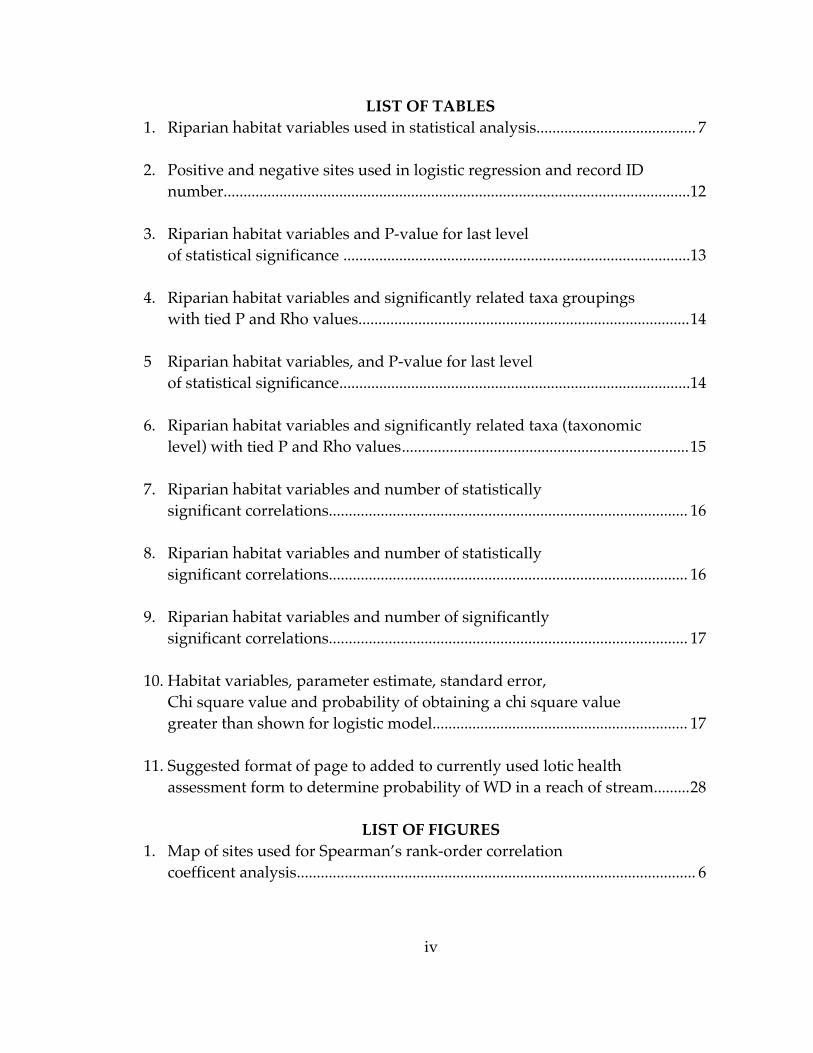
LIST OF TABLES1. Riparian habitat variables used in statistical analysis........................................ 7
2. Positive and negative sites used in logistic regression and record ID number.....................................................................................................................12
3. Riparian habitat variables and P-value for last levelof statistical significance .......................................................................................13
4. Riparian habitat variables and significantly related taxa groupingswith tied P and Rho values...................................................................................14
5 Riparian habitat variables, and P-value for last levelof statistical significance........................................................................................14
6. Riparian habitat variables and significantly related taxa (taxonomiclevel) with tied P and Rho values........................................................................15
7. Riparian habitat variables and number of statisticallysignificant correlations.......................................................................................... 16
8. Riparian habitat variables and number of statisticallysignificant correlations.......................................................................................... 16
9. Riparian habitat variables and number of significantlysignificant correlations.......................................................................................... 17
10. Habitat variables, parameter estimate, standard error,Chi square value and probability of obtaining a chi square valuegreater than shown for logistic model................................................................ 17
11. Suggested format of page to added to currently used lotic healthassessment form to determine probability of WD in a reach of stream.........28
LIST OF FIGURES1. Map of sites used for Spearman’s rank-order correlation
coefficent analysis.................................................................................................... 6
iv

APPENDICESA Sampling sites eliminated from analysis and reason for
elimination....................................................................................................... A1
GLOSSARYGlossary ......................................................................................................................G1
v

INTRODUCTION
Whirling disease (WD) is the common name for a condition in salmonids caused
by infection by the microscopic parasite Myxobolus cerebralis. This parasite has a
complex life cycle involving two hosts and assumes two different forms. The
spore form of the parasite is released when an infected fish dies. Spores are
ingested by worms of the genus Tubifex. After a few months inside the worm, the
parasite changes into a free swimming infective stage called a TAM, and is
released into the water column. It infects a fish host to complete its life cycle
(Rocky Mountain Fly Fishing Center 1996).
Once inside a young fish, M. cerebralis attacks the cartilage. Young fish are most
vulnerable because they possess large amounts of soft cartilage. Adult fish are
less affected because once cartilage has hardened they show few ill effects of
infection. In severe infections, inflammation around the damaged cartilage places
pressure on the nervous system, causing the fish to “whirl” when startled. Spinal
deformities can also result. Seriously infected fish have a reduced ability to feed
or escape from predators (Markiw 1992). Although all species of trout and
salmon are susceptible to WD, rainbow trout populations seem to be the most
devastated.
The impact of WD on trout fisheries, especially in the western United States, has
been devastating. Colorado reports wild rainbow population declines in the
Colorado, Gunnison, Arkansas, Rio Grande, South Platte and Poudre rivers
(Marlowe and Gardner 1995). Rainbow populations in Montana’s Madison River
have decreased from 3,300 per mile to 300 per mile (Marlowe and Gardner 1995).
WD has been confirmed in Montana’s Ruby River, Clark Fork River, Rock Creek
1

and others for a total of 73 rivers, streams and lakes (Montana Fish, Wildlife and
Parks 1999). Rivers in other states have been similarly impacted.
Waddington and Laughland (1996) indicate that in Montana, average angler
expenditure per day is $66. It is estimated that fishermen spend about 2.3 million
angler days per year pursuing trout in Montana (McFarland 1995.) This revenue,
much of it spent in local economies, could be seriously impacted by WD.
The 1996 Whirling Disease Conference in Denver, CO, developed a list of five
ecological factors which appear to influence presence of the disease and potential
for populational impacts. All sites that test positive for WD:
1. Are highly productive, i.e., over 300 pounds/acre (this is standing crop and
Wetzel, 1983, defines this as the weight of organic material that can be sampled
or harvested at any one time from a given area) and commonly have very high
electrical conductivity readings.
2. Have flushing flows less than one out of ten years.
3. Have brown trout present to act as a reservoir for the disease. (The parasite is
from Europe where it co-evolved with brown trout. These trout show little
symptoms of the disease, but function as carriers.)
4. Are relatively low gradient streams.
5. Have human-altered or enriched habitats which amplify the pathogen.
In a keynote address at the 1999 Whirling Disease Symposium held in Missoula,
MT, Allendorf (1999), stated habitat degradation may cause stress on fish. This
stress may make fish more susceptible to the disease by weakening them.
2

Spring creeks, tail water streams and disturbed streams and rivers are considered
to be high risk for WD (Gustafson 1996). Conversely, undisturbed Rocky
Mountain streams and rivers, warm trout waters (above the critical higher
temperature limit for TAMs) and lake outlets (too cold for TAMs) are listed as
low risk areas.
Within these general ecological factors influencing the presence or absence of
WD, there is much to be discovered. This study attempts to identify the specific
ecological factors that support conditions conducive to WD by using benthic
macroinvertebrate data indicative of disturbance in streams. Use of benthic
macroinvertebrates to monitor and assess biological condition in the Pacific
Northwest is an accepted approach (Fore and others 1996.) The goal of such
biological monitoring and assessment often is to measure and evaluate the
consequences of human actions on biological systems (Karr and Chu 1999).
Determining these factors and being able to scale their importance will provide
managers a tool for dealing with WD. Additionally, if criteria for these
ecological factors could be used to predict probability of a stream reach
supporting WD, evaluation procedures could be developed that would enable
managers to evaluate a reach of stream, determine problem areas, and plan
remedial efforts accordingly.
Specific Study Goals
Specific goals of this study are:
1. Construct a list of habitat variables ranked in their importance to presence or
absence of WD in a stream.
2. Relate the score generated by the ranked habitat variables to incidence of WD.
3
Whirling disease is a fact of life in America and is here to stay (Vincent 1999).
While WD can not be eliminated, it may be controlled, especially in the small
feeder streams where salmonids hatch. If control methods can be developed,
fisheries in the western states can be maintained.
Developing effective control methods will involve several steps:
1. Identifying riparian habitat variables that influence presence or absence of
WD.
2. Scaling importance of those variables.
3. Designing an assessment procedure that would enable managers to evaluate
streams within their purview and estimate probability of those streams
supporting WD.
4

METHODS AND MATERIALS
Data
Data for analyses were provided by the Bureau of Land Management (BLM) and
collected by an independent contractor. Data were for 185 sites in the montane
ecoregion of western Montana (Omernik and Gallant 1986). A total of 40 sites
were eliminated from analysis to maintain data consistency (Appendix A).
Figure 1 shows the 145 sites used.
Nilson (1998) describes collection procedures for benthic macroinvertebrates
used in this study. Relevant details follow.
Collection times—Late fall and early spring are the appropriate times to collect
mature Tubifex. Identification of Tubifex worms requires mature specimens. The
worms mature in late fall and in spring are washed away from their habitat
during heavy runoff. Tubifex worms were sampled in the spring and fall of 1997,
and spring of 1998.
Site selection—BLM 1:100,000 surface management maps were used for site
selection. Road access was considered in determining sample sites. The number
of sites sampled on a given stream was determined by how much of the stream
was on BLM land. Majority of sites sampled were on BLM land but a few
additional Forest Service and private sites were sampled. Sites were selected to
provide an overall view of a stream. Riparian areas in degraded condition
received special attention.
5

Figure 1. Map of sites used for analysis
6

Riparian habitat variables—Nine riparian habitat variables were measured and
used in statistical analyses. Table 1 provides a list of these riparian habitat
variables and numbers.
Table 1. Riparian habitat variables and numbers used in statistical analysis______________________________________________________________________________________
Habitat Variable Variable Number______________________________________________________________________________________
Amount of flood plain and stream banks covered by plant 1growthPercent of stream bank bound by a deep root mass 2Percent of riparian zone covered by noxious weeds 3Percent of the site covered by disturbance-induced 4undesirable herbaceous speciesDegree of browse utilization of trees and shrubs 5Woody species establishment and regeneration 6Percent of site with human caused bare ground 7Percent of stream bank structurally altered by humans 8Incisement (vertical stability of the channel) 9
______________________________________________________________________________________
Sampling procedure—Once a site representative of upstream and downstream
reaches was selected, the following data was obtained:
1. A GPS reading, utilizing a Magellan GPS 2000 XL or 3000XL, was taken and
additional readings determined 25 ft upstream and downstream to delineate
upper and lower boundaries of the sample site.
2. Riparian health assessment form was filled out in accordance with Thompson
and others (1998). The following information was added to each assessment
form:
• Rosgen stream type (Rosgen 1996)
• Benthic macroinvertebrate sample number (macro ID number)
• Section, township and range
• Macro stream habitat types (shoreline, undercut banks, sediment, gravel,
cobble, boulder, bedrock, submerged vegetation, woody debris)
• Comments
• Valley type (subjective description by sampler)7

3. At each site an ocular estimation of macro stream habitat types was made.
Each stream habitat type was assigned a percentage of total stream sample area
and sampled in its representative percentage by kick net.
4. Sample material was placed in sifting buckets and non-benthic
macroinvertebrate material removed. Remainder of sample was placed in 500 ml
containers and preserved with ethanol.
5. When large macroinvertebrates stopped movement, 50 ml formalin was added
to each 500 ml container.
6. Each container received a waterproof identification tag with benthic
macroinvertebrate sample number and stream name.
7. Each container was then sealed and labeled again using a strip of freezer
paper.
Scores for riparian habitat variables were calculated using the Riparian and
Wetlands Research Program’s (RWRP) lotic health assessment (stand alone) form
in accordance with Thompson and others (1998). These scores provide a
quantified health assessment for each site. Riparian habitat variables for each site
were scored at the same time and place as benthic macroinvertebrates for each
site were collected.
Benthic macroinvertebrates were identified and placed into taxonomic groupings
by the National Aquatic Monitoring Center at Utah State University, Logan,
Utah. A full description of protocols used to identify and classify benthic
macroinvertebrates used for analysis in this study can be found at their web site:
www.usu.edu/~buglab under aquatic invertebrate sampling protocols, option
two.
8

Analysis Methods
Method # 1—Spearman’s rank-order correlation coefficient analysis, a non-
parametric procedure, was utilized to calculate correlations between scores for
nine individual habitat variables, total riparian rating and taxonomic category.
Statview statistical software (Abacus Concepts 1996) was used to perform this
procedure. This statistical procedure investigates whether there is a monotomic
relationship between two variables (Sheskin 1997) and requires no assumption of
normality or independence of variables.
The correlation coefficient, Rho, provides a measure of strength of the
monotomic relationship between two variables even if that relationship is not
linear (Ott 1993). Perfect positive relationships show a Rho score of positive one
while perfect negative relationships display a Rho score of negative one.
Complete lack of correlation is indicated by zero.
Statistical strength of the Rho statistic is defined by a p-value with scores from
zero to one. Smaller p-values indicate greater statistical significance. Tied Rho
and p-values vs. basic Rho and p-values were utilized to strengthen conclusions
of analyses. Use of basic Rho and p-values can cause inflation of statistical
significance (Sheskin 1997). Tied values in either scores for riparian habitat
variables, overall riparian score or taxonomic data were corrected by assigning to
each tied observation the mean rank of the rank positions for which it is tied
(Daniel 1990).
A total of 650 Spearman’s rank order correlation coefficient analyses were
conducted between nine habitat variables, total riparian rating, and 65 taxa
9

groupings indicative of disturbance in streams. A spreadsheet of results for each
Spearman analysis was constructed. With 650 values and a p-value of 0.05 set as
necessary for significance, as many as 32 spurious correlations could result. To
avoid this, a Bonferroni-Dunn test was performed with a familywise Type I error
rate set at 0.05 (Sheskin 1997). This procedure adjusts p-values to eliminate
spurious correlations as number of correlations increases. As a result of this test,
a p-value of less than or equal to 0.0001 was established as necessary to maintain
a true p-value of 0.05.
Spearman analyses were also performed between habitat variables, total riparian
rating, and individual benthic macroinvertebrate data used to determine
taxonomic groupings. This was done to ensure relationships between individual
taxa and habitat variables were not masked by inclusion of individual taxa in a
taxa grouping. Data for 205 individual taxa were provided and each of these
were run against nine habitat variables and an overall score for a total of 2,050
Spearman rank order correlation analyses.
A Bonnferroni-Dunn test with a familywise Type I error set at 0.05 (Sheskin 1997)
was utilized to determine the p-value necessary to maintain a true p-value of 0.05
for the 2,050 analyses. This procedure established 0.000024 as the correct p-value
to maintain a p-value of 0.05. Statview (Abacus Concepts 1996) sets < 0.0001 as
minimum p-value it will compute. However, 0.00001, lowest increment to five
decimal places is lower than 0.000024. Using < 0.0001, as provided by Statview, is
more rigorous than required.
Method # 2—Because presence or absence of whirling disease is a binary
response to habitat variables determined to be significantly tied to disturbance in
10
streams, a logistic regression model is appropriate (Hosmer and Lemeshow
1989). JMP (SAS Institute 1995), a statistical software package, was used to fit a
logistic regression model that estimates the probability of stream reaches having
or being capable of supporting whirling disease based on habitat variable scores.
Sites used to provide data for logistic regression were selected by matching sites
with benthic macroinvertebrate samples provided by the BLM with sites listed as
tested for whirling disease by Montana Fish, Wildlife & Parks (1999). A total of
35 data points, 15 with WD and 25 without, were used to construct the logistic
model and are included as Table 2.
11

Table 2. Positive and negative sites used in logistic regression and record ID number______________________________________________________________________________________Record ID Number Positive sites Negative sites______________________________________________________________________________________006 X009 X010 X013 X029 X031 X038 X072 X108 X113 X115 X142 X143 X154 X174 X003 X011 X016 X018 X023 X026 X027 X070 X071 X090 X091 X092 X093 X094 X095 X096 X097 X098 X104 X106 X146 X168 X173 X187 X190 X______________________________________________________________________________________
12

RESULTS
Analysis Method # 1
Table 1 provides a list of riparian habitat variables and numbers used in
statistical analyses. With a p-value of less than or equal to 0.0001 required to be
statistically significant for correlation of taxa groupings with habitat variables,
four habitat variables were eliminated (Table 3). None of these variables are
correlated with groupings of benthic macroinvertebrates indicative of
disturbance in streams with a level of significance satisfying the minimum of
less than or equal to 0.0001. Table 3 lists these variables, and p-values for the last
level of significance met by the variable before being eliminated.
Table 3. Riparian habitat variables, numbers, and P-value for last level of statistical significance ______________________________________________________________________________________
Habitat Variable Variable Number P-value______________________________________________________________________________________
Percent of stream bank bound by 2 0.1a deep root massPercent of stream bank structurally 8 0.025altered by humansPercent of riparian zone covered 3 0.005by noxious weedsAmount of flood plain and stream 1 0.001banks covered by plant growth
______________________________________________________________________________________
With a p-value less than or equal to 0.0001, the following five habitat variables
remain:
• Percent of the site covered by disturbance-induced undesirable herbaceous
species (variable # 4)
• Degree of browse utilization of trees and shrubs (variable # 5)
• Woody species establishment and regeneration (variable # 6)
• Percent of site with human caused bare ground (variable # 7)
• Incisement (vertical stability of the channel) (variable # 9)
13

Table 4 displays variable number, taxonomic groupings with statistically
significant correlations, and tied p and Rho values for the correlation.
Table 4. Habitat variable numbers, significantly related taxa groupings with tied p and Rho values______________________________________________________________________________________
Variable Taxa Groupings P-values Rho values______________________________________________________________________________________
4 # intolerant taxa <0.0001 +0.3755 # intolerant taxa <0.0001 +0.4086 Intolerant taxa abundance <0.0001 +0.414
# intolerant taxa <0.0001 +0.382Plecoptera abundance <0.0001 +0.336EPT taxa 0.0001 +0.320Mollusca taxa <0.0001 -0.366CTQ:d <0.0001 -0.387# tolerant taxa <0.0001 -0.422
7 Scraper abundance <0.0001 +0.3899 Scraper abundance <0.0001 +0.370
______________________________________________________________________________________Values at top and bottom of each variable represents strongest positive and negative correlations where applicable.
With a p-value of < 0.0001 established as minimum for significant correlation
between individual benthic macroinvertebrate taxa and habitat variables to be
significant, five habitat variables are eliminated. Table 5 shows these habitat
variables, and P-values for the last level of significance met by the variable before
being eliminated.
Table 5. Riparian habitat variables, and p-value for last level of statistical significance______________________________________________________________________________________
Habitat Variable Variable Number P-value______________________________________________________________________________________
Percent of streambank structurally 8 0.0036 altered by humans
Incisement (vertical stability of the 9 0.0016 channel)
Percent of streambank bound by a 2 0.0010 deep root mass
Amount of the floodplain and stream 1 0.0007 banks covered by plant growth.
Percent of site with human caused 7 0.0002 bare ground
______________________________________________________________________________________
14

With a p-value < 0.0001, four habitat variables remain:
• Percent of the riparian zone covered by noxious weeds (variable # 3)
• Percent of the site covered by disturbance-induced undesirable herbaceous
species (variable # 4)
• Degree of browse utilization of trees and shrubs (variable # 5)
• Woody species establishment and regeneration (variable # 6)
Table 6 displays habitat variable number, taxa with statistically significant
correlations, and tied p and Rho values for the correlation.
Table 6. Habitat variable numbers, significantly related taxa (taxonomic level) with tied p and Rho values______________________________________________________________________________________Habitat Variable Taxa P-values Rho values
Number______________________________________________________________________________________
3 Capniidae <0.0001 +0.356Ephemerella infrequens <0.0001 -0.520
4 Ephemerella infrequens <0.0001 +0.459Nemouridae <0.0001 +0.366Prosimulium <0.0001 +0.361
5 Nemouridae <0.0001 +0.360Ephemerella infrequens <0.0001 +0.347Epeorus <0.0001 +0.325Ephemerella <0.0001 -0.418
6 Epeorus <0.0001 +0.421Rhyacophila <0.0001 +0.419Sweltsa <0.0001 +0.396Helicopsyche <0.0001 -0.329Physella <0.0001 -0.348
______________________________________________________________________________________Values at top and bottom of each variable represent strongest positive and negative correlations where applicable.
Table 7 displays riparian habitat variables, and number of statistically significant
correlations to taxa groupings indicative of disturbance in streams for each
variable.
15

Table 7. Riparian habitat variables their numbers, and number of statistically significant correlations ______________________________________________________________________________________
Habitat Variable Variable Number of statisticallyNumber significant correlations
to taxa groupings indicative of disturbance
______________________________________________________________________________________Percent of the site covered by 4 1
disturbance-induced undesirableherbaceous species
Degree of browse utilization of 5 1 trees and shrubs
Woody species establishment and 6 7 regeneration
Percent of site with human caused 7 1 bare ground
Incisement (vertical stability of the 9 1 channel)
______________________________________________________________________________________
Table 8 shows riparian habitat variables, and number of statistically significant
correlations to individual taxa.
Table 8. Riparian habitat variables their numbers, and number of statistically significant correlations______________________________________________________________________________________
Variable Variable Number of statisticallyNumber significant correlations
to taxa groupings indicative of disturbance
______________________________________________________________________________________Percent of the riparian zone covered 3 2
by noxious weedsPercent of the site covered by 4 3
disturbance-induced undesirable herbaceous species
Degree of browse utilization of 5 4 trees and shrubs
Woody species establishment and 6 5 regeneration
______________________________________________________________________________________
Table 9 combines results shown in Tables 7 and 8. It displays riparian habitat
variables, number of statistically significant correlations to taxa groupings
indicative of disturbance in streams for each variable, number of statistically
16

significant correlations to individual taxa for each variable, and total number of
statistically significant correlations for each variable.
Table 9. Riparian habitat variable numbers and number of statistically significant correlations ______________________________________________________________________________________
Variable Number of statistically Number of statistically Total number of Number significant correlation significant correlations statistically significant
to taxa groupings to individual taxa correlations for eachindicative of variabledisturbance in streams
______________________________________________________________________________________3 0 2 24 1 3 45 1 4 56 7 5 127 1 0 19 1 0 1
______________________________________________________________________________________
Analysis Method # 2
A logistic regression model provided by JMP (SAS 1995) utilizing presence or
absence of whirling disease as the dependent variable and scores for habitat
variables listed in Tables 4 and 6 as independent variables yielded the results
shown in Table 10.
Table 10. Habitat variable numbers, parameter estimate, standard error, Chi squarevalue and probability of obtaining a chi square value greater than shown for logistic model______________________________________________________________________________________
Variable Parameter Standard Chi Prob > ChiNumber Estimate Error Square Square
______________________________________________________________________________________3 + 0.01 0.21 0.00 0.95014 + 0.59 0.85 0.49 0.48625 - 0.32 0.39 0.67 0.41376 + 0.36 0.34 1.10 0.29347 + 0.31 0.24 1.59 0.20799 - 0.68 0.35 3.60 0.0577
______________________________________________________________________________________
17

DISCUSSION
There is an association between incidence of WD and human impacted streams
(Gustafson 1996). One of five ecological factors identified as associated with WD
by the 1996 Whirling Disease Conference is human altered or enriched habitats.
Habitat degradation may stress fish making them more susceptible to disease
and changes in stream habitat may increase abundance of Tubifex tubifex,
alternate host of M. cerebralis. (Allendorf 1999).
Identifying variables in degraded habitats important to incidence of WD gives
managers a tool to help control the disease. Utilizing benthic macroinvertebrate
data, in groupings that reflect riparian health is an effective way to validate those
variables. Both variables and taxonomic data are measures of disturbance in
streams where whirling disease is found. I was able to identify five measurable
habitat variables linked with strong statistical significance to benthic
macroinvertebrate groupings indicating disturbance in streams (Table 3).
Utilizing individual taxa vs. taxonomic groupings in analysis with habitat
variables and overall health scores may yield relationships masked by an
individual taxa’s inclusion in a group. Such relationships can provide another
link between disturbance in a stream and habitat variables, and therefore with
whirling disease. I found four riparian habitat variables with strong correlations
to individual taxa (Table 5).
Thompson and others (1998) provide instructions for measuring the habitat
variables listed in Tables 4 and 6. As riparian health increases, scores for
applicable variables increase. Table 4 provides tied Rho values that are measures
18

of correlation between variables and listed taxa groupings indicative of
disturbance. Thompson and others (1998) provide instructions for measuring the
habitat variables listed in Tables 4 and 6. As riparian health increases, scores for
applicable variables increase. Table 4 provides tied Rho values that are measures
of correlation between variables and listed taxa groupings indicative of
disturbance in streams. Table 6 provides tied Rho values that are measures of
correlation between variables and listed individual taxa. Negative correlation
values are inversely related to increasing health while positive correlations are
directly related to increasing health values.
Table 8 lists each riparian habitat variable that has significant statistical
correlations to either taxa groupings indicative of riparian health or individual
taxa and total number of significant statistical correlations. Each of these riparian
habitat variables and its significant correlations will be discussed in order.
Percent of Riparian Zone Covered by Noxious Weeds (Variable # 3)
This habitat variable has significant statistical links with Capniidae, a family of
Plecoptera (stoneflies), and with Ephemerella infrequens , a species of
Ephemeroptera (mayfly). As the health rating for this particular variable
increases, the percent of noxious weeds decreases. Numbers of Capniidae
increase as health ratings increase. This positive correlation was expected since
Plecoptera are generally associated with cool, clean water (Stewart and Harper
1996) and increasing health scores indicate such conditions.
Congenerics of Ephemerella infrequens include 32 species of insects which feed as
collector-gatherers and scrapers. E. infrequens, ,however, is a shredder (Edmunds
19

and Waltz 1996). Wisseman (1990) states shredders are indicative of a healthy
riparian vegetation community; however numbers of E. infrequens decrease as
riparian health scores for percent of noxious weeds increase. Although we view
noxious weeds as undesirable and assign lower health scores as their presence
increases, E. infrequens uses noxious weeds only as riparian plants. Cummins
and others (1989) state shredders do not feed specifically on litter of a particular
species, but rather on appropriately conditioned litter, regardless of species.
Strong negative correlation with health scores in this instance reflects a strong
positive correlation with the presence of riparian vegetation, and is an indicator
of good health.
Percent of the Site Covered by Disturbance-Induced Undesirable Herbaceous
Species (Variable # 4)
This variable has a positive correlation with number of intolerant taxa. As health
score increases, so do the number of intolerant taxa. This relationship was as
expected.
Habitat variable # 4 is statistically linked to three individual taxa. Strongest of
these statistical links is a positive correlation with E. infrequens. Undesirable
herbaceous species indicate displacement from potential natural community and
are less productive and generally have shallow roots. They poorly perform most
riparian functions (Thompson and others 1998). Positive correlation with health
scores indicates an increase in E. infrequens numbers as health score increases.
Nemouridae, a family of Plecoptera, is positively tied to health scores for variable
# 4. Their numbers should and do increase as health score increases.
20

Riparian health variable # 4 is also positively correlated with Prosimulium, a
genus of Diptera (true flies). Hilsenhoff (1988) rates Simulidae, the family
containing Prosimulium, as moderately intolerant, but the same author (1987)
listed three species of genus Prosimulium as very intolerant and two as
moderately intolerant. A positive correlation with health scores is consistent with
his ratings for intolerance.
Degree of Browse Utilization of Trees and Shrubs (Variable # 5)
Like riparian habitat # 4, this variable also has a strong positive correlation with
number of intolerant taxa. As health score increases, so do number of intolerant
taxa.
This riparian habitat variable also has four significant statistical ties to individual
benthic macroinvertebrate taxa. For this variable, health scores increase as
browse utilization decreases. Three of four taxa linked to this variable have
positive correlations while one is negative.
Of three positively correlated taxa, two, Nemouridae (a family of Plecoptera) and
E. infrequens, have been discussed relative to riparian habitat variable #4. That
discussion applies to degree of browse utilization also. The third, Epeorus, is in
Ephemeroptera in the family Heptageniidae. Winget and Magnum (1979) and
Wisseman (1990) both list Epeorus spp. as intolerant so their numbers would be
expected to increase as health scores increase. The positive correlation found
confirms this.
21

Ephemerella, a genus in the family Ephemerelladae in Ephemeroptera, is
negatively correlated to degree of browse utilization. Edmunds and Waltz (1996)
describe Ephemerella, a genus with 32 species, as mostly collector-gatherers with
some scrapers. Wisseman (1990) states collector-gatherers feed on fine sediment
enriched with particles of organic matter and that when collector-gatherers
increase, it is an indicator of declining water quality. A negative correlation
between Ephemerella and riparian health is expected.
Woody Species Establishment and Regeneration (Variable # 6)
This riparian habitat variable has seven statistically significant correlations with
taxa groupings indicative of disturbance in streams. Four of these correlations
are positive and three negative.
Intolerant taxa abundance number and associated number of intolerant taxa have
a strong positive correlation to health scores. As health score increases, so does
number of intolerant taxa and intolerant taxa abundance. Plecoptera abundance
and Ephemerella Plecoptera Tricoptera (EPT) taxa are also related and also show
a positive correlation. Bode (1988) and Wisseman (1990) state EPT richness is
indicative of disturbance in a stream and is positively tied to health, i.e., EPT taxa
richness increases as health increases. Correlation values in Table 3 reflect that
relationship.
Mollusca taxa, CTQ:d (a community tolerance quotient), and number of tolerant
taxa show negative correlations to riparian health. As health scores increase,
these taxa decrease. Mollusca do well in organically enriched habitats with high
sediment (Harmon 1974) which indicates disturbance. Winget and Mangum
22

(1979) list the entire phylum Mollusca as highly tolerant of disturbance. A
negative correlation as shown in Table 4, therefore, was expected. CTQ:d and
number of tolerant taxa should both decrease as riparian health increases.
Negative correlations indicate they do. Of five significant correlations with
individual benthic macroinvertebrate taxa, three are positive and two negative.
Epeoreus, a genus of mayflies considered to be intolerant (Winget and Mangum
1979; Wisseman 1990) has the strongest positive correlation. This was expected
and is discussed above with respect to habitat variable # 5.
Rhyacophila, in Tricoptera (caddis flies) and in the family Rhyacophilidae, is tied
positively to woody species establishment and regeneration. Hilsenhoff (1988)
assigns the family, Rhyacophilidae, a zero tolerance level and Winget and
Magnum (1979) rate the genus Rhyacophila equal with the family. A strong
positive correlation between Rhyacophila and habitat variable # 6 indicates this
highly intolerant genus increases with increasing health..
A Plecopteran, Sweltsa, also shows a strong positive relationship with woody
species establishment and regeneration. Hilsenhoff (1988) assigns this genus an
intolerant rating and Winget and Magnum (1979) give it a low tolerance rating.
Both these ratings are in keeping with the positive correlation that was found.
Helicopsyche, a second Trichopteran genus and Physella, a gastropoda in the
Phylum Mollusca, both exhibit negative correlations with woody species
establishment and regeneration. Helicopsyche is a member of the family
Heliocopsychidae which Hilsenhoff (1988) lists as relatively intolerant to
23

pollution. However, Helicopsyche is considered an algal grazer (Williams and
others 1983; Wiggins 1996). Vaughn, (pers. com. 1999) suggests that as woody
species grow in riparian zones, they provide shade for streams and shading
eliminates or reduces periphyton on rocks. This is completely consistent with the
negative correlation with woody shrub establishment and regeneration. As
shrubs increase in riparian zones along stream banks, shade increases,
periphyton decreases and numbers of Helicopsyche will decline.
Winget and Mangum (1979) list the entire phylum Mollusca as highly tolerant.
Harmon (1974) describes the family Physidae, which contains Physella , as one of
two most resistant families in the entire Phylum. It is no surprise that their
numbers decline as health scores for woody establishment and regeneration
increase.
Percent of Site With Human Caused Bare Ground (Variable # 7)
This riparian habitat variable has a positive significant correlation to the benthic
macroinvertebrate functional group “scrapers.” Wisseman (1990) discusses the
functional group scrapers and concludes a diverse and numerically well
represented scraper community reflects good habitat/water quality. My analyses
indicate a positive relationship as is shown in Table 4.
Incisement (Vertical Stability of the Channel) (Variable # 9)
This variable has only one statistically significant correlation and this correlation
is a positive one to the functional group “scrapers.” As discussed above with
respect to variable # 7, a numerically well represented scraper community
indicates good habitat/water quality.
24

Riparian Habitat Variables and Disturbance
Riparian habitat variable #6, woody species establishment and regeneration, was
the most important indicator of disturbance in streams. There are 12 significant
ties to disturbance indicative benthic macroinvertebrate data. Degree of browse
utilization of trees and shrubs (riparian habitat variable # 5) has five significant
links with benthic macroinvertebrate data and is second most important. It is
clearly tied to woody species establishment and regeneration.
High browse utilization however accomplished, will prevent woody species
from establishment and regeneration. Woody plant species increase rapidly
when riparian areas are protected from livestock grazing (Schulz and Leninger
1990). Kauffman and others (1983) conclude excess browsing does not allow
woody species to regenerate and Kauffman and Krueger (1984) state excessive
grazing pressures prevent establishment of seedlings. Sixty-eight percent of
statistically significant ties between riparian habitat variables and benthic
macroinvertebrate data indicative of stream health are accounted for by these
two riparian habitat variables (variables # 5 and # 6).
Habitat variable # 4 (percentage of site covered by disturbance-induced
undesirable herbaceous species) accounts for an additional four significant links
between riparian habitat variables and disturbance indicative benthic
macroinvertebrates. Platts (1978) states livestock trample and compact the soil
resulting in loss of high-quality, fibular-rooted plants. These are replaced by
shallow rooted annual species or taprooted forbs and shrubs. These generally
continue to increase with continued grazing because they are unpalatable.
Ohmart (1996) concludes that after a few years of grazing, the herbaceous
25

ground cover mix changes from highly palatable, better soil holding species to
less, or even non-palatable, shallow rooted annuals and perennials. They
contribute to stream degradation because they do not perform well the role of
riparian vegetation (Thompson and others 1998). These four links added to the
12 links associated with habitat variable six and five links with habitat variable
five indicate 84 percent of statistically significant ties between benthic
macroinvertebrate data and disturbance are associated with grazing.
Habitat variable # 3 (percent of riparian zone covered by noxious weeds) has an
additional two links to disturbance indicative benthic macroinvertebrate data.
Young and Evans (1989) have tied deteriorated range conditions due to grazing
to spread of noxious weeds in Nevada. These two links, added to the above, give
92 percent of riparian habitat variables associated with disturbance as also
associated with disturbance caused by grazing.
Percent of human-caused bare ground, habitat variable # 7, is strongly associated
with grazing by Schulz and Leininger (1990.) They state grazed areas in their
study had four times more bare ground than ungrazed areas. Adding this link to
ones discussed above increases percentage of statistically significant links
between benthic macroinvertebrate data and disturbance to 96 percent strongly
linked to grazing.
Livestock are attracted to riparian areas because of lush foliage, shade and water,
especially in hotter arid months (Ohmart 1996; Skovlin 1984). Fleischner (1994)
states livestock grazing is the most widespread land management practice in
western North America and that 70 percent of this area is grazed. He further
states that ecological implications of grazing can be dramatic. Szaro (1989) feels
26

that degradation of many riparian systems and overgrazing by domestic
livestock are integrally related. Armour and others (1994) feel overgrazing by
domestic livestock was one of the principal factors contributing to damage and
loss of riparian and stream ecosystems in the West. Elmore (1992) attributes
degradation and elimination of many riparian systems to improper grazing
practices.
In addition to general riparian degradation caused by livestock grazing, the
specific cause and effect relationship of riparian vegetation removal and
increases in stream temperature is critical. As vegetation is removed and streams
lose shading, stream temperatures increase (Ohmart 1996; Beschta 1991; Brazier
and Brown 1973). WD shows a significant correlation between intensity of
infection and daily mean water temperature (Vincent 1999.)
Habitat variable # 6 (woody species establishment and regeneration) and habitat
variable #5 (degree of browse utilization of trees and shrubs) have a total of 17
significant links with benthic macroinvertebrate data indicative of disturbance.
This represents 68 percent of total significant links and are clearly tied to grazing.
If woody species in these areas were allowed to regenerate, stream temperatures
would be lowered and infection rate for WD lessened.
Logistic Regression
Parameter estimates listed in Table 9, results of logistic regression modeling, are
actually weighting factors for the habitat variables associated with them.
Multiplying scores for each habitat variable listed by its parameter provides a
weighted and signed (positive or negative) score for that variable. Summing
these scores for each site provides the probability that the stream or reach of
stream for which the habitat assessment was done, has or will support WD.
27

Table 11 is a suggested format of a page to be added to the currently used lotic
health assessment form that can be used to determine probability of WD in a
reach of stream:
Table 11 . Suggested format to be added to currently used lotic health assessment form that can be used to determine probability of WD in a reach of stream______________________________________________________________________________________
Score for habitat variable # 3 ______ X 0.01 = ______Score for habitat variable # 4 ______ X 0.59 = ______Score for habitat variable # 6 ______ X 0.36 = ______Score for habitat variable #7 ______ X 0.31 = ______
Subtotal A ______
Score for habitat variable #5 ______ X 0.32 = ______Score for habitat variable #9 ______ X 0.68 = ______
Subtotal B ______
Subtotal A ______
Minus Subtotal B ______
Probability of WD ______
______________________________________________________________________________________
Although the additional page for the lotic health assessment form as illustrated
above provides some predictive power, it is limited for the following reasons:
1. Dates Montana Department of Fish, Wildlife and Parks (MTDFWP)
determined presence or absence of WD do not coincide with the dates benthic
macroinvertebrate samples used in this study were collected. These dates differ
by two years in some cases. For meaningful statistical analysis of the presence or
absence of WD relative to benthic macroinvertebrate samples, sampling and the
determination of WD presence must be accomplished at the same time.
2. Benthic macroinvertebrates were collected on the same streams that MTFWP 28

determined presence or absence of WD. However, the location of sampling sites
for benthic macroinvertebrates and sites used to determine presence of WD were
different. For valid ststistical analysis locations must be the same.
Recommendations to improve predictive power of the logistic regression model
are included under suggestions for future research.
Unhealthy streams support the presence of WD. The type of disturbance caused
by improper grazing appears to be especially critical to the presence or absence
of the disease. Changes in composition of the vegetative community and
presence of a healthy “woody” component of that community can be directly
linked to grazing. Lack of trees and shrubs in a riparian zone also contribute to
temperature regulation of a stream and this is crucial to the TAM phase in the
life cycle of the parasite.
The assessment protocol developed by logistic regression, when refined by
future research, will allow managers to determine if a stream, or reach of stream,
will support WD. Additionally, this procedure will provide managers with a list
of strong and weak points for remedial action
29

SUMMARY
Analysis Method # 1
Of nine habitat variables considered in this study, six have significant statistical
links with disturbance in streams and hence with WD:
• Woody species establishment and regeneration (variable # 6)
• Degree of browse utilization of trees and shrubs (variable # 5)
• Percent of the site covered by disturbance induced undesirable herbaceous
species (variable # 4)
• Percent of the riparian zone covered by noxious weeds (variable # 3)
• Percent of site with human caused bare ground (variable # 7)
• Incisement (vertical stability of the channel) (variable # 9)
Variables are ranked by total number of significant links with benthic
macroinvertebrate data indicative of disturbance.
Analysis Method # 2
Logistical regression enables an assessment procedure to be generated that will
give the probability that a reach of stream has or will support WD. A suggested
format is provided in the discussion section as Figure 2.
Additional Conclusion
There is a strong association between WD and disturbance caused by grazing.
Ninety-six percent of statistical links between riparian habitat variables and
benthic macroinvertebrate data indicative of disturbance can be attributed to
grazing, whether by livestock or wildlife.
30

SUGGESTIONS FOR FUTURE RESEARCH
1. The logistic regression model developed in this study lacks sufficient
predictive power for reasons discussed previously. To overcome this problem, it
is recommended that an additional research project be conducted. This project
should provide for a site to be assessed according to previously developed
methods (Thompson and others 1998.) Benthic macroinvertebrate samples
should be collected at the same time and place as the assessment. Additionally,
presence or absence of WD at that site at that time should be determined through
analysis of gut contents of T. tubifex collected at the site for presence of M.
cerebralis.
2. It was noted during research and analysis of data for this study that the
caddisfly, Helicopsyche borealis, may well possess attributes allowing it to be used
as an indicator species. It is easily recognizable because of its unique snail
shaped shell constructed of sand grains and has transcontinental distribution
(Resh and others 1984).
As noted in the discussion section, this caddisfly is an algal grazer and increases
with increased periphyton. It also has high tolerance for increased thermal
conditions (Vaughn 1984). Further, T. tubifex is difficult to identify while H.
borealis is simple. More importantly, H. borealis should increase as shrubby
riparian vegetation decreases and water temperature and periphyton increases.
The combination of these characteristics make larvae of this benthic
macroinvertebrate a possible candidate as an indicator species.
When benthic macroinvertebrate samples are collected, correlations between H.
borealis, T. tubifex, and presence or absence of WD should be examined.
31

ACKNOWLEDGEMENTS
Funding and data for this project was provided by the Bureau of Land
Management through the efforts of Dan Hinckley, Riparian and Wetland
Coordinator for the BLM Montana State Office.
Dr. Paul Hansen of the Riparian and Wetland Research Program, the University
of Montana, was my major professor throughout this project and offered
invaluable advice, suggestions, and encouragement. He gave an old veteran a
chance and changed my life.
Drs. Colin Henderson and Diana Six were on my graduate committee and
provided more help than I had any right to expect.
My wife and my mother never gave up on me. If you think women are the
weaker sex, you never met them.
32

LITERATURE CITED
Abacus Concepts, Inc. 1996. Statview. Berkeley, CA. 268 p.
Allendorf, Fred. 1999. Genetics, wild trout, and whirling disease: first do no harm. pp.1-3. In : Proceedings. Whirling Disease Symposium:Research and Management Perspectives. Missoula, MT. Whirling Disease Foundation, Bozeman, MT.
Armour, C. L., D. Duff and W. Elmore. 1994. The effects of livestock grazing on western riparian and stream ecosystems. Journal of American Fish Society 19: 9-12.
Beschta, Robert. 1991. Stream habitat management for fish in the northwestern United States: the role of riparian vegetation. American Fisheries Society Symposium 10: 53-58.
Bode, Robert W. 1988. Methods for rapid biological assessment of streams. New York State Department of Environmental Conservation. Albany, NY. 27 p.
Brazier, Jon R. and George W. Brown. 1973. Buffer strips for stream temperature control. Research Paper 15, Oregon State University. Corvallis, Oregon. 9 p.
Cummins, K. W., M. A. Witzbach, D. M. Gates, J. B. Perry and W. B. Taliafero. 1989. Shredders and riparian vegetation. Bioscience 39(1): 24-30.
Daniel, Wayne W. 1990. Applied nonparametric statistics. 2d ed. PWS-KENT Publishing Company, Boston, MA. 635 p.
Edmunds, G. F. and R. D. Waltz. 1996. Ephemeroptera. In: An introduction to the aquatic insects of North America. 3rd ed. R.W. Merritt and K.W. Cummins (eds.) Kendall/Hunt Publishing, Dubuque, IA. pp. 126-163.
Elmore, Wayne. 1992. Riparian responses to grazing practices. pp 442-457 In:Watershed management: balancing sustainability and environmental change. R. J. Naiman, editor. Springer-Verlag, New York, NY.
Fleischner, T. L. 1994. Ecological costs of livestock grazing in western North America. Conservation Biology 8(3):629-644.
Fore, L. S., J. R, Karr and R. W. Wisseman. 1996. Assessing invertebrate responses to human activity: evaluating alternative approaches. Journal of North American Benthological Society 15:212-231.
33

Gustafson, D. L. 1996. Montana whirling disease positive sites. http://rivers.oscs.montana.edu/dlg/aim/annelid/wpositive.
Harmon, Willard N. 1974. Snails (Mollusca: Gastropoda). In: Pollution ecology of freshwater invertebrates. Edited by C. W. Hart and Samuel L. H. Fuller. Academic Press, New York, NY. pp 275-312.
Hilsenhoff, W. L. 1987. An improved biotic index of organic stream pollution. The Great Lakes Entomologist 20 (1):31-39.
Hilsenhoff, W. L. 1988. Rapid field assessment of organic pollution with a family level biotic index. Journal of North American Benthological Society 7(1): 65-68.
Hosmer, David W, and Stanley Lemeshow. 1989. Applied Logistic Regression. John Wiley and sons, New York. NY. 307 p.
Karr, James R. and Ellen W. Chu. 1999. Restoring life in running waters: better biological monitoring. Island Press, Washington, DC. 206 p.
Kauffman, J. Boone., W. C. Krueger, and M. Vavra. 1983. Effects of cattle grazing on riparian plant communities. Journal of Range Management. 36: 685-691.
Kauffman, J. Boone and W. C. Krueger. 1984. Livestock impacts on riparian ecosystems and streamside management implications...a review. Journal of Range Management 37(5):430-438.
Markiw, E. 1992. Salmonid whirling disease. U.S. Fish and Wildlife Service Leaflet 17.
Marlowe, A. and Hugh Gardner. 1995. Whirling disease in the Rockies. Rocky Mountain Streamside, Spring Issue, p. 17. Denver CO.
McFarland, Robert. 1995. Montana statewide angling pressure 1991. Montana Department of Fish, Wildlife and Parks. Helena, MT. 112 p.
Montana Fish, Wildlife and Parks. 1999. Montana waters tested for Myxobolus cerebralis since December 1994. Great Falls, MT. 56 p.
Nilson, Robert. 1998. 1997-1998 Macro Invertebrate (sic) Field Sampling. Unpublished letter to Bureau of Land Management, Montana State Office,Billings, MT, Whirling Disease Project, received 5 June 1998.
34

Ohmart, Robert D. 1996. Historical and present impacts of livestock grazing on fish and wildlife resources in western riparian habitats. In: Rangeland Wildlife, P. R. Krausman, ed. Society for Range Management, Denver, CO. pp.245-279.
Omernik, J. M. and A. L. Gallant. 1986. Ecoregions of the Pacific Northwest. US EPA Publication 600/3-86/033. Corvallis Environmental Research Laboratory. Corvallis, OR. 39p.
Ott, R. Lyman. 1993. An introduction to statistical methods and data analysis, 4th ed. Wadsworth Publishing Company, Belmont, CA. 1,051 p.
Platts, William S. 1978. Livestock grazing and riparian/stream ecosystems- an overview. In: Grazing and riparian/stream ecosystems: Proceedings of the Forum in Denver, Colorado, November 3-4, 1978 by Trout Unlimited, Inc.
Resh, Vincent H., Gary A Lamberti and John R. Wood. 1984. Biology of the caddis fly Helicopsyche borealis (Hagen): a comparison of North American populations. Freshwater Invertebrate Biology 3(4):172-180.
Rocky Mountain Fly Fishing Center, 1996. Whirling Disease facts Page. http://www.xmission.com/gastown/flyfishing/facts.html
Rosgen, Dave. 1996. Applied river morphology. Wildland Hydrology, Pagosa Springs, CO. 333 p.
SAS Institute, Inc. 1995. JMP Statistics and graphics guide, Version 3. Cary, NC. 593p.
Schulz, Terri T. and Wayne C. Leninger. 1990. Differences in riparian vegetation structure between grazed areas and enclosures. Journal of Range Management 43(4):295-299.
Sheskin, D. J. 1997. Handbook of parametric and non parametric statistical procedures. CRC Press, New York, NY. 719 p.
Skovlin, Jon M. 1984. Impacts of grazing on wetlands and riparian habitat: a review of our knowledge. Pages 1001-1103 In: Developing strategies for rangeland management. National Research Council/National Academy of Sciences. Westview Press, Boulder, Colorado.
Stewart, K. W. and P. P. Harper. 1996. Plecoptera. In: An introduction to the aquatic insects of North America. 3d ed. R. W. Merritt and K. W. Cummins (eds.) Kendall/Hunt Publishing, Dubuque, IA. pp. 217-266.
35

Szaro, Robert C. 1989. Riparian forest and shrubland community types of Arizona and New Mexico. Rocky Mountain Forest and Experiment Station. Tempe, AZ. 138 p.
Thompson, W. H., R. C. Ehrhart, P. L. Hansen, T. G. Parker and W. C. Haglan. 1998 Assessing health of a riparian site. In: Rangeland Management and Water Resources, Proceedings, AWRA Specialty Conference. May 27 29, Reno, NV.
Vaughn, Caryn. 1999. Director and Associate Professor, Oklahoma Biological Survey and Department of Zoology, University of Oklahoma. Personal e-mail. 30 Mar 1999.
Vaughn, Caryn. 1984. Ecology of Helicopsyche borealis (Hagen) (Tricoptera: Helicopsychidae): life history and microdistribution. Ph. D. Dissertation, The University of Oklahoma. 93 p.
Vincent, E. Richard. 1999. How the relationship between water temperature and the intensity of Myxobolus cerebralis infections can be used in management solutions. In: Proceedings. Whirling Disease Symposium: Research and Management Perspectives. Missoula, MT. Whirling Disease Foundation, Bozeman, MT. pp. 211-213 .
Waddington, D. and A. Laughland. 1996. Trout fishing in the U.S. Report 91-5. U.S. Fish and Wildlife Service, Washington, D.C. 17 p.
Wetzel, Robert G. 1983. Limnology. Saunders college Publishing, Orlando, FL. 767 p.
Wiggins, G. B. 1996. Larvae of the North American caddis fly genera. 2d ed.Univ. Toronto Press. 401p.
Williams, D. D., A. T. Read, and K. A. Moore. 1983. The biology andzoogeography of Helicopsyche borealis (Tricoptera: Helicopsychidae): a Neararctic representative of a tropical genus. Canadian Journal of Zoology 61:2288-2299.
Wingett, R. N. and F. A. Mangum. 1979. Biotic condition index: integrated biological, physical, and chemical parameters for management. U.S. Forest Service Intermountain Region, U.S. Department of Agriculture, Ogden, UT. 51 p.
Wisseman, R. W. 1990. Montana rapid bioassessment protocols, benthic macro invertebrate studies, 1990, Demonstration Projects. Aquatic Biology Associates, Corvallis, Oregon. Report to Montana Water Quality Bureau. 82 p.
Young, J. A. and R. A. Evans. 1989. Silver State rangelands-historical perspective. Rangelands 11:199-203.
36

Appendix A
Sampling Sites Eliminated From Analysis Listed By Record ID NumberAnd Reason Eliminated
A1

Record ID Number Reason Eliminated000 No health scores, not included in data base015 no health scores028 no elevation029 “047 no lat/long, elev.048 “049 “070 “073 “076 “084 no Hill’s evenness092 no elevation096 no lat/long, elev.105 no elevation106 “107 “108 “109 “111 “112 “113 “114 “115 “116 “117 “118 “154 no lat/long, elev.155 “156 “157 “158 “159 “160 “161 “162 “163 “164 “165 “166 “167 “
A2

Glossary
Collector-gatherers. A functional feeding group of benthic macroinvertebrates that feed on fine sediment that is enriched with particles of organic matter.
CTQ:d. A community tolerance quotient used by the Forest Service.
EPT. Ephemeroptera+Plecoptera+Tricoptera (Mayflies+Stoneflies+Caddisflies) are orders of aquatic insects.
Functional feeding group. A group of insects that feed in the same manner.
Gatherers. A functional feeding group of benthic macroinvertebrates that feed on sediments.
Scrapers. A functional feeding group that acquires its food by grazing periphyton (microfloral growth) off hard surfaces found on the bottom of streams.
Shredders. A functional feeding group of benthic macroinvertebrates that consumes large particles of detritus.
G1


![Restoring Salmonid Aquatic/Riparian Habitat...aquatic/riparian habitat restoration activities. [5] [6] VISION AND OBJECTIVES The overreaching goal of this initiative is to improve](https://img.pdfslide.us/doc/110x75/6104737c127ac45d1972c9a7/restoring-salmonid-aquaticriparian-habitat-aquaticriparian-habitat-restoration.jpg)