Embed Size (px)
Citation preview
RELATING FUTURE COASTAL CONDITIONS TO EXISTING FEMA FLOOD HAZARD MAPS
Technical Methods Manual
Prepared for October 2016 California Department of Water Resources and California Ocean Science Trust
RELATING FUTURE COASTAL CONDITIONS TO EXISTING FEMA FLOOD HAZARD MAPS
Technical Methods Manual
Prepared for October 2016 California Department of Water Resources and California Ocean Science Trust
Prepared by
Robert T. Battalio, PE1, Peter D. Bromirski2, Daniel R. Cayan3, Louis A. White, PE1
Citation Battalio, R. T., P. D. Bromirski, D. R. Cayan, L. A. White (2016). Relating Future Coastal Conditions to Existing FEMA Flood Hazard Maps: Technical Methods Manual, Prepared for California Department of Water Resources and California Ocean Science Trust, Prepared by Environmental Science Associates (ESA), pp. 114. 550 Kearny Street Suite 800 San Francisco, CA 94108 415.896.5900 www.esassoc.com
Los Angeles
Oakland
Orlando
Palm Springs
Petaluma
Portland
Sacramento
San Diego
Santa Cruz
Seattle
Tampa
Woodland Hills
D130028.29 / 208177.03 / 150306.00
1 Environmental Science Associates 2 Climate, Atmospheric Sciences, and Physical Oceanography Division, Scripps Institution of Oceanography, University of California, San Diego, La Jolla, California,
USA. 3 Climate Research Division, Scripps Institution of Oceanography and U.S. Geological Survey, La Jolla, California, USA.
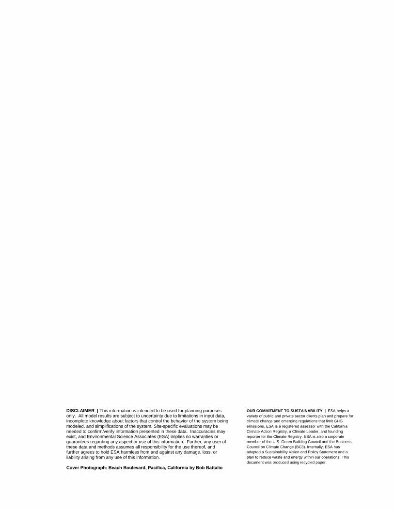
DISCLAIMER | This information is intended to be used for planning purposes only. All model results are subject to uncertainty due to limitations in input data, incomplete knowledge about factors that control the behavior of the system being modeled, and simplifications of the system. Site-specific evaluations may be needed to confirm/verify information presented in these data. Inaccuracies may exist, and Environmental Science Associates (ESA) implies no warranties or guarantees regarding any aspect or use of this information. Further, any user of these data and methods assumes all responsibility for the use thereof, and further agrees to hold ESA harmless from and against any damage, loss, or liability arising from any use of this information. Cover Photograph: Beach Boulevard, Pacifica, California by Bob Battalio
OUR COMMITMENT TO SUSTAINABILITY | ESA helps a
variety of public and private sector clients plan and prepare for
climate change and emerging regulations that limit GHG
emissions. ESA is a registered assessor with the California
Climate Action Registry, a Climate Leader, and founding
reporter for the Climate Registry. ESA is also a corporate
member of the U.S. Green Building Council and the Business
Council on Climate Change (BC3). Internally, ESA has
adopted a Sustainability Vision and Policy Statement and a
plan to reduce waste and energy within our operations. This
document was produced using recycled paper.

Relating Future Coastal Conditions to Existing FEMA Flood Hazard Maps i ESA / 208177.03 / 150306.00
Technical Methods Manual October 2016
TABLE OF CONTENTS
Technical Methods Manual
1. Introduction 1-1 1.1 Background 1-2
2. Coastal Flooding Parameters 2-1 2.1 Terminology 2-1 2.2 Runup Equations 2-3
3. Methods to Adjust FEMA Maps for Sea Level Rise 3-1 3.1 Using FEMA Hazard Maps to Identify Future Flood Hazards Related to Sea Level Rise 3-1 3.2 Level 2 Adjust V-Zones 3-2 3.3 Considering Geomorphic Change 3-14 3.4 Accounting for Coastal Armoring Structures 3-17
4. Examples 4-1 4.1 Example of Level 1 Comparison 4-2 4.2 Example of Level 2a Add Sea Level Rise to Adjust V Zone 4-4 4.3 Example of Level 2b Prorate TWL to Adjust V Zone 4-7
5. Recommendations 5-1
6. References 6-1
7. Acknowledgements 7-1 7.1 Study authors 7-1 7.2 Clients and Co-Study authors 7-1 7.3 Focus Group participants 7-1 7.4 Technical Methods Manual Committee Participants 7-2
Appendices
A. An Overview of FEMA Flood Insurance Studies and Flood Insurance Rate Maps A-1
B. Scripps Institution of Oceanography (SIO) Future Waves and Water Levels B-1
B1. Extreme Value Analysis on Scripps Institute of Oceanography Data B1-1 B2. Extreme Value Analysis on Observed Data B2-1
C. Other Sea Level Rise Hazard Mapping Studies and Sources C-1
D. Additional information available from FEMA to support Method 2b of this TMM D-1
Table of Contents
Relating Future Coastal Conditions to Existing FEMA Flood Hazard Maps ii ESA / 208177.03 / 150306.00
Technical Methods Manual October 2016
List of Tables
2.1 Slope Terminology 2-2 3.1 Morphology Function Summary 3-8 4.1 Comparison of Existing and Future Twls 4-4 4.2 Summary of Wave Existing and Future Extreme Wave Runup Computed
for the Obmp 4-8 5.1 Morphology Function Recommendations 5-2 B.1 Climate Model Simulations Used to Predict Water Levels and Waves B-3 B.2 Climate Scenarios Consistent with Nrc (2012) Sea Level Rise Projections B-4 B.3 Proposed Time Horizons B-4 B.4 Sea Level Rise Scenarios from Nrc (2012) in Cm B-5 B.5 Future Total Water Levels Ocean Beach, San Francisco (Meters, Msl) B-11 B.6 Future Projected and Measured Historical Data Sources Compared B-12 B.7 Extreme Water Levels Computed from Observations and Model Output. B-18 C.1 Coastal Hazard Model Selection Criteria and Comparison Table C-2 List of Figures
2.1 Definitions 2-2 2.2 Slope Schematic 2-3 2.3 Typical cross section for TAW runup equation 2-4 2.4 Plot of the TAW Runup Equations in Non-Dimensional Form 2-5 2.5 Wave Setup Terms, Dynamic and Incident Wave Runup 2-6 2.6 2.6a. Shows How the Components that Influence TWL Change Across the
Surfzone, and 2.6b Shows the Composite Slope Method that is Applicable to Most California Coasts Where Wave Setup from Larger Waves Maximize Total Water Levels 2-7
2.7 Cumulative Distribution of Total Water Level at Ocean Beach, San Francisco 2-9
3.1 Shore Morphology Response to Sea Level Rise and Effect on Total Water Level for Erodible and Erosion Resistant Backshores 3-4
3.2 Plot of Relative Shore Recession for a Shore Face Depth of 40 Feet and a Range of Reduction Factor “a” Values Associated with Backshore Sand Contributions 3-5
3.3 Graph of Non-Dimensional Wave Runup on Steep Slopes 3-6 3.4 TWL Response to SLR on Non-Erodible Backshores with Depth-Limited
Breaking Waves 3-7 3.5 Bore Propagation Driven by Wave Runup above the Shore Elevation 3-9 3.6 Expanded inland extent of wave action due to increased overtopping for a
range of negative freeboard of ΔRfuture/ΔRexisting between 1.1 and 3 and Yexisting between 5 and 100 feet. 3-9
3.7 Landward extent of wave runup for Bay and Open Coast Conditions using the Cox and Machemehl and Composite Slope models 3-10
3.8 Proration Schematic 3-12 3.9 2008 FEMA Map and 2009 Future Conditions Erosion Hazard Map 3-15 3.10 Historical Coastal Erosion Rates Derived from USGS using DSAS 3-16 4.1 FEMA Preliminary FIRM, South Ocean Beach, San Francisco 4-2 4.2 FEMA Preliminary FIRM, South Ocean Beach, San Francisco 4-3 4.3 Level 2a Example, 3’ of SLR 4-5 4.4 Profiles of the Shore and Near-Shore of Ocean Beach in the area at Rivera
Street, Characterized by a Sandy Dune Backshore 4-8
Table of Contents
Relating Future Coastal Conditions to Existing FEMA Flood Hazard Maps iii ESA / 208177.03 / 150306.00
Technical Methods Manual October 2016
4.5 Profiles of the Shore and Near-Shore of Ocean Beach in the Area South of Sloat Boulevard 4-9
A.1 Parameters Used to Determine Flood Hazard Zones on FEMA Maps A-2 A.2 Flood Hazard Zone Calculation Methodology A-3 A.3 Shore Section Schematic Showing Coastal Hazard Zonation A-5 A.4 Example of a Workmap Used to Develop a Flood Hazard Map A-5 A.5 FEMA Flood Maps for Seadrift, Stinson Beach A-6 A.6 Provisional FEMA Flood Map for Seadrift, Stinson Beach, CA A-7 B.1 Location of Offshore Wave and Nearshore Total Water Level Forecast
Locations B-2 B.2 Example of TWL Results without Sea Level Rise B-3 B.3 Sea Level Rise Curves for this Project based on NR B-6 B.4 Future Sea Level Time Series for San Francisco B-7 B.5 Future Projected Wave Height for Ocean Beach B-7 B.6 Wave Runup Time Series for Ocean Beach B-8 B.7 Wave Runup Time Series for Ocean Beach using the Stockdon Equation B-8 B.8 Total Water Level (TWL) Time Series for Ocean Beach, San Francisco B-9 B.9 Wave height time series for Ocean Beach, San Francisco for Different
GCMs B-10 B.10 Total Water Level (TWL) Time Series for Ocean Beach, San Francisco B-10 B.11 Cumulative Distribution of Ocean Reference Water Level for Projected SIO
GCM and Real Data B-13 B.12 Cumulative Distributions of Calculated Runup Heights for SIO GCM and
Observed Data at Harvest Buoy and a Range of Beach Slopes B-14 B.13 Time Series of Total Water Levels for SIO GCM and Observed Data at
Various Foreshore Beach Slopes B-15 B.14 Cumulative Distributions of Total Water Level for SIO GCM and Observed
Data Using Stockdon and TAW Models for Various Foreshore Beach Slopes B-16
B.15 Extreme Value Distributions Fit to Annual Maximum Total Water Level for SIO GCM Projections and Observed Data for Several Foreshore Beach Slopes B-17
B.17 Composite Slope Method Applicable to Most California Coasts Where Wave Setup from Larger Waves Maximize Total Water Levels B-19
B.18 Cumulative Distribution of Total Water Level at Ocean Beach, San Francisco Comparing SIO GCM and Real Data Calculated with Stockdon and a Modified TAW Approach B-21
Table of Contents
Relating Future Coastal Conditions to Existing FEMA Flood Hazard Maps iv ESA / 208177.03 / 150306.00
Technical Methods Manual October 2016
This page intentionally left blank
Relating Future Coastal Conditions to Existing FEMA Flood Hazard Maps 1-1 ESA / 208177.03 / 150306.00
Technical Methods Manual October 2016
CHAPTER 1
Introduction
The purpose of this Technical Methods Manual (TMM or Manual), Relating Future Coastal
Conditions to Existing FEMA Flood Hazard Maps, is to help planners and engineers
approximately adjust FEMA coastal flood maps to account for higher sea levels anticipated to
occur in the future. This project is focused on California where the State has provided guidance
to account for sea level rise in coastal zone planning and permitting, future coastal hazards are
being mapped throughout the State, and municipalities are struggling with application of the
future conditions maps. While focused on California, the “gap” between existing and future
coastal hazard mapping will emerge for other coastal states in the near future. This TMM is
focused on part of this “gap”: Specifically, relating future conditions flood maps to existing
conditions FEMA maps for planning purposes. Scripps Institution of Oceanography (SIO)
provided future wave and water level projections and wave runup calculations to support this
study. These data were compared to historic data to discern the predicted change in coastal flood
levels that result from secular sea level rise as well as meteorological and climatic effects on
short-term ocean water levels and wave conditions. This TMM is organized as follows:
Chapter 2. Coastal Flooding Parameters provides a description of sea levels, wave
runup and total water levels used in coastal flood hazard mapping, along with definitions
and equations.
Chapter 3. Methods to Adjust FEMA Maps for Sea Level Rise describes how flood
hazards shown on FEMA maps can be approximately adjusted for sea level rise.
Chapter 4. Examples provides examples of applications of the methods described in
Chapter 3.
Chapter 5 Recommendations identifies actions to improve reporting of existing and
future coastal hazards to facilitate their combined use in planning.
Appendix A. Federal Emergency Management Agency (FEMA) Flood Insurance
Studies (FISs) and Flood Insurance Rate Maps (FIRMs) provides a summary
description of FEMA coastal flood maps.
Appendix B. Scripps Institution of Oceanography (SIO) Future Waves and Water
Levels summarizes the SIO modeling used in this study. In addition, summaries of future
and historic data are organized for use:
Appendix B1. SIO Future Projections provides selected future coastal flood
levels developed by Scripps Institution of Oceanography (SIO) for this study.
Appendix B2. Historical Data provides computed water levels, wave runup
heights and total water levels using real tide and wave gauge data.
1. Introduction
Relating Future Coastal Conditions to Existing FEMA Flood Hazard Maps 1-2 ESA / 208177.03 / 150306.00
Technical Methods Manual October 2016
Appendix C. Other Sea Level Rise Hazard Mapping Studies and Sources is a summary
of other future coastal hazard mapping sources in California.
1.1 Background
Outreach funded by a National Oceanic and Atmospheric Administration (NOAA) Climate Grant
identified an acute need to understand how to use future conditions coastal hazard maps, and how
to relate these maps to Federal Emergency Management Agency (FEMA) existing conditions
flood maps. 4 This TMM was developed in response to this expressed need. However, there
remains a significant institutional gap which this TMM cannot fill. In particular, it is not possible
to assign any authority or sanction to this TMM other than its contribution to subsequent Federal
and or State guidance. This document will speed the development of such guidance, and does
thereby contribute to more effective planning for sea level rise.
As presently constituted, FEMA does not address climate change impacts in the National Flood
Insurance Program (NFIP), although there is a general provision allowing program applicants to
consider “expected future conditions” in the context of program compliance. Consequently, this
study was designed to provide a background to support local planners in taking sea-level rise and
additional coastal processes such as erosion into account as part of assessing risk of coastal
flooding.
This Manual, Relating Future Coastal Conditions to Existing FEMA Flood Hazard Maps, relates
future coastal conditions from modeling conducted by the Scripps Institution of Oceanography
(SIO) to existing conditions coastal flood maps produced by the FEMA in order to inform
mapping of future coastal hazards needed to conduct local planning. This Manual also provides
methods for relating future coastal conditions projected by other modeling and research efforts to
FEMA Flood Hazard Maps, in addition to the SIO projections. In addition to assisting application
of the SIO projections, the TMM is intended as a resource for users to apply and investigate other
projections of coastal conditions made using alternative approaches or different and newly-
emerging information.
This Manual was developed as part of a multi-agency effort5 funded by the NOAA Coastal and
Ocean Climate Adaptation (COCA) Program, The California Department of Water Resources
(DWR) with coordination support from the California Ocean Science Trust (OST), to develop
guidance products to help local communities adapt and plan for sea level rise. The Manual was
developed by Environmental Science Associates (ESA) and Scripps Institution of Oceanography
(SIO) scientists with input from OST, DWR, and broad participation by professionals active in
coastal engineering, planning and management (see Acknowledgements). A Focus Group,
comprised of 17 agencies across local, State and Federal governments, provided oversight of the
effort, and a Technical Methods Manual Committee (TMMC) provided more detailed review and
input.
4 OST, 2015: Needs Assessment. 5 Piloting Non-Stationary Approaches to Floodplain Management: Supporting Local Communities and Informing
National Policy.
Relating Future Coastal Conditions to Existing FEMA Flood Hazard Maps 2-1 ESA / 208177.03 / 150306.00
Technical Methods Manual October 2016
CHAPTER 2
Coastal Flooding Parameters
2.1 Terminology
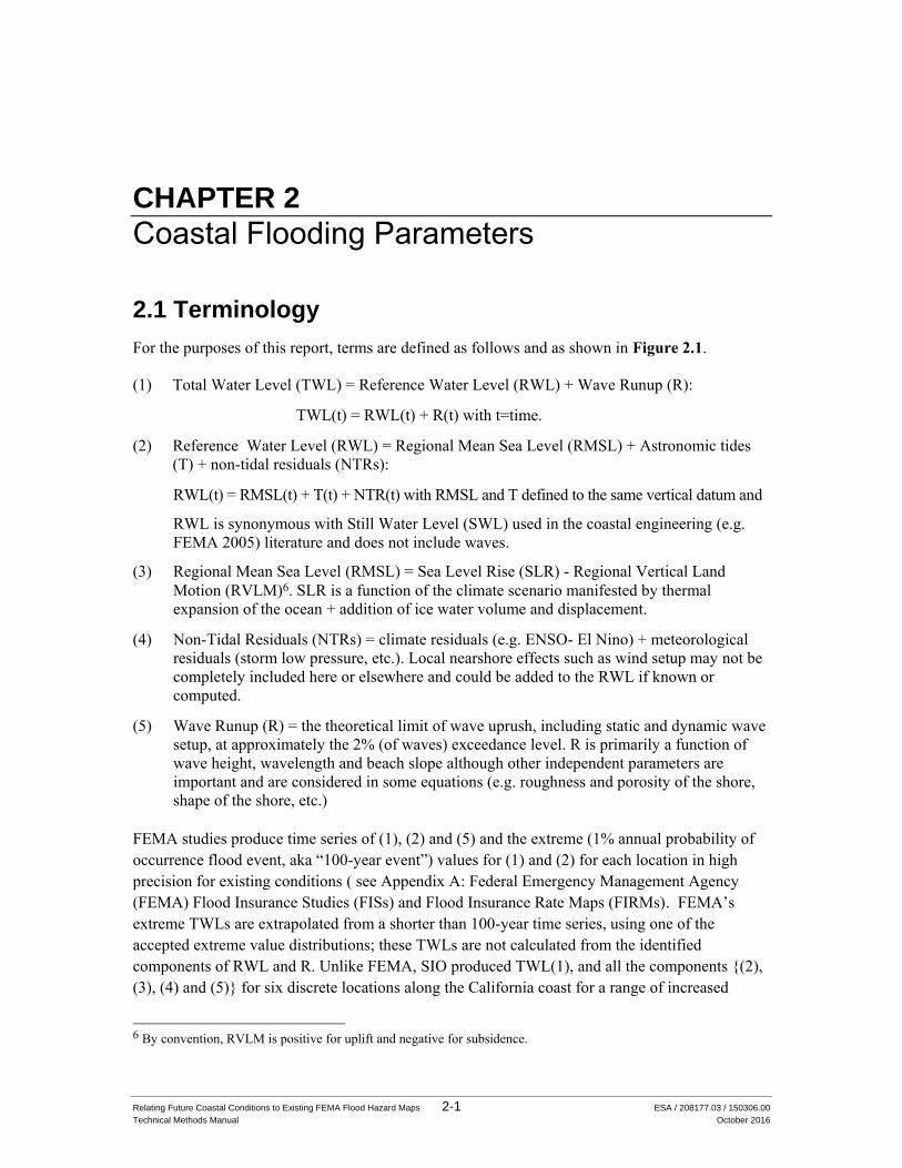
For the purposes of this report, terms are defined as follows and as shown in Figure 2.1.
(1) Total Water Level (TWL) = Reference Water Level (RWL) + Wave Runup (R):
TWL(t) = RWL(t) + R(t) with t=time.
(2) Reference Water Level (RWL) = Regional Mean Sea Level (RMSL) + Astronomic tides
(T) + non-tidal residuals (NTRs):
RWL(t) = RMSL(t) + T(t) + NTR(t) with RMSL and T defined to the same vertical datum and
RWL is synonymous with Still Water Level (SWL) used in the coastal engineering (e.g.
FEMA 2005) literature and does not include waves.
(3) Regional Mean Sea Level (RMSL) = Sea Level Rise (SLR) - Regional Vertical Land
Motion (RVLM)6. SLR is a function of the climate scenario manifested by thermal
expansion of the ocean + addition of ice water volume and displacement.
(4) Non-Tidal Residuals (NTRs) = climate residuals (e.g. ENSO- El Nino) + meteorological
residuals (storm low pressure, etc.). Local nearshore effects such as wind setup may not be
completely included here or elsewhere and could be added to the RWL if known or
computed.
(5) Wave Runup (R) = the theoretical limit of wave uprush, including static and dynamic wave
setup, at approximately the 2% (of waves) exceedance level. R is primarily a function of
wave height, wavelength and beach slope although other independent parameters are
important and are considered in some equations (e.g. roughness and porosity of the shore,
shape of the shore, etc.)
FEMA studies produce time series of (1), (2) and (5) and the extreme (1% annual probability of
occurrence flood event, aka “100-year event”) values for (1) and (2) for each location in high
precision for existing conditions ( see Appendix A: Federal Emergency Management Agency
(FEMA) Flood Insurance Studies (FISs) and Flood Insurance Rate Maps (FIRMs). FEMA’s
extreme TWLs are extrapolated from a shorter than 100-year time series, using one of the
accepted extreme value distributions; these TWLs are not calculated from the identified
components of RWL and R. Unlike FEMA, SIO produced TWL(1), and all the components {(2),
(3), (4) and (5)} for six discrete locations along the California coast for a range of increased
6 By convention, RVLM is positive for uplift and negative for subsidence.
2. Coastal Flooding Parameters
Relating Future Coastal Conditions to Existing FEMA Flood Hazard Maps 2-2 ESA / 208177.03 / 150306.00
Technical Methods Manual October 2016
global energy (emissions) scenarios for a range of future times. SIO used a simplified TWL index
based on a beach runup equation (the Stockdon equation) for a range of beach slopes (see
Appendix B: Scripps Institution of Oceanography (SIO) Future Waves and Water Levels).
Figure 2.1 Definitions
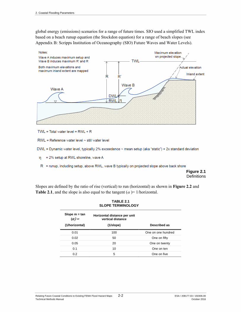
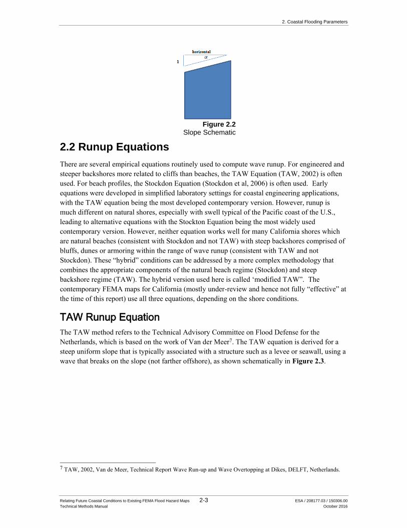
Slopes are defined by the ratio of rise (vertical) to run (horizontal) as shown in Figure 2.2 and
Table 2.1, and the slope is also equal to the tangent ( )= 1/horizontal.
TABLE 2.1 SLOPE TERMINOLOGY
Slope m = tan
(
(1/horizontal)
Horizontal distance per unit vertical distance
(1/slope) Described as
0.01 100 One on one hundred
0.02 50 One on fifty
0.05 20 One on twenty
0.1 10 One on ten
0.2 5 One on five
2. Coastal Flooding Parameters
Relating Future Coastal Conditions to Existing FEMA Flood Hazard Maps 2-3 ESA / 208177.03 / 150306.00
Technical Methods Manual October 2016
Figure 2.2
Slope Schematic
2.2 Runup Equations
There are several empirical equations routinely used to compute wave runup. For engineered and
steeper backshores more related to cliffs than beaches, the TAW Equation (TAW, 2002) is often
used. For beach profiles, the Stockdon Equation (Stockdon et al, 2006) is often used. Early
equations were developed in simplified laboratory settings for coastal engineering applications,
with the TAW equation being the most developed contemporary version. However, runup is
much different on natural shores, especially with swell typical of the Pacific coast of the U.S.,
leading to alternative equations with the Stockton Equation being the most widely used
contemporary version. However, neither equation works well for many California shores which
are natural beaches (consistent with Stockdon and not TAW) with steep backshores comprised of
bluffs, dunes or armoring within the range of wave runup (consistent with TAW and not
Stockdon). These “hybrid” conditions can be addressed by a more complex methodology that
combines the appropriate components of the natural beach regime (Stockdon) and steep
backshore regime (TAW). The hybrid version used here is called ‘modified TAW”. The
contemporary FEMA maps for California (mostly under-review and hence not fully “effective” at
the time of this report) use all three equations, depending on the shore conditions.
TAW Runup Equation
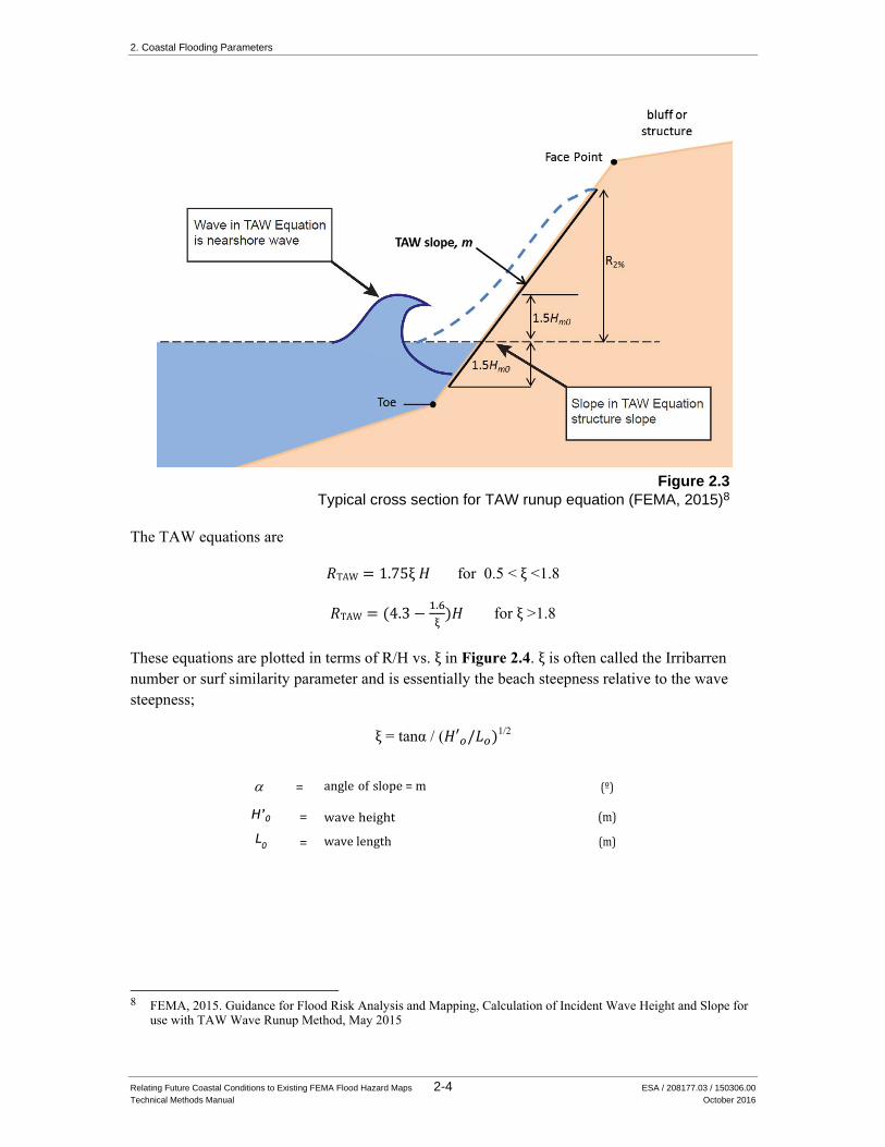
The TAW method refers to the Technical Advisory Committee on Flood Defense for the
Netherlands, which is based on the work of Van der Meer7. The TAW equation is derived for a
steep uniform slope that is typically associated with a structure such as a levee or seawall, using a
wave that breaks on the slope (not farther offshore), as shown schematically in Figure 2.3.
7 TAW, 2002, Van de Meer, Technical Report Wave Run-up and Wave Overtopping at Dikes, DELFT, Netherlands.
2. Coastal Flooding Parameters
Relating Future Coastal Conditions to Existing FEMA Flood Hazard Maps 2-4 ESA / 208177.03 / 150306.00
Technical Methods Manual October 2016
Figure 2.3
Typical cross section for TAW runup equation (FEMA, 2015)8
The TAW equations are
𝑅TAW = 1.75ξ 𝐻 for 0.5 < ξ <1.8
𝑅TAW = (4.3 −1.6
ξ)𝐻 for ξ >1.8
These equations are plotted in terms of R/H vs. ξ in Figure 2.4. ξ is often called the Irribarren
number or surf similarity parameter and is essentially the beach steepness relative to the wave
steepness;
ξ = tanα / (𝐻′𝑜/𝐿𝑜)1/2
= angle of slope = m (º)
H’0 = wave height (m)
L0 = wave length (m)
8 FEMA, 2015. Guidance for Flood Risk Analysis and Mapping, Calculation of Incident Wave Height and Slope for
use with TAW Wave Runup Method, May 2015
2. Coastal Flooding Parameters
Relating Future Coastal Conditions to Existing FEMA Flood Hazard Maps 2-5 ESA / 208177.03 / 150306.00
Technical Methods Manual October 2016
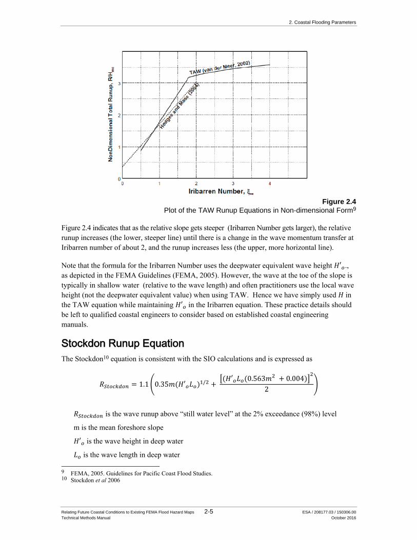
Figure 2.4
Plot of the TAW Runup Equations in Non-dimensional Form9
Figure 2.4 indicates that as the relative slope gets steeper (Iribarren Number gets larger), the relative
runup increases (the lower, steeper line) until there is a change in the wave momentum transfer at
Iribarren number of about 2, and the runup increases less (the upper, more horizontal line).
Note that the formula for the Iribarren Number uses the deepwater equivalent wave height 𝐻′𝑜.,
as depicted in the FEMA Guidelines (FEMA, 2005). However, the wave at the toe of the slope is
typically in shallow water (relative to the wave length) and often practitioners use the local wave
height (not the deepwater equivalent value) when using TAW. Hence we have simply used 𝐻 in
the TAW equation while maintaining 𝐻′𝑜 in the Iribarren equation. These practice details should
be left to qualified coastal engineers to consider based on established coastal engineering
manuals.
Stockdon Runup Equation
The Stockdon10 equation is consistent with the SIO calculations and is expressed as
𝑅𝑆𝑡𝑜𝑐𝑘𝑑𝑜𝑛 = 1.1 (0.35𝑚(𝐻′𝑜𝐿𝑜)1/2 + [(𝐻′𝑜𝐿𝑜(0.563𝑚2 + 0.004)]
2
2)
𝑅𝑆𝑡𝑜𝑐𝑘𝑑𝑜𝑛 is the wave runup above “still water level” at the 2% exceedance (98%) level
m is the mean foreshore slope
𝐻′𝑜 is the wave height in deep water
𝐿𝑜 is the wave length in deep water
9 FEMA, 2005. Guidelines for Pacific Coast Flood Studies. 10 Stockdon et al 2006
2. Coastal Flooding Parameters
Relating Future Coastal Conditions to Existing FEMA Flood Hazard Maps 2-6 ESA / 208177.03 / 150306.00
Technical Methods Manual October 2016
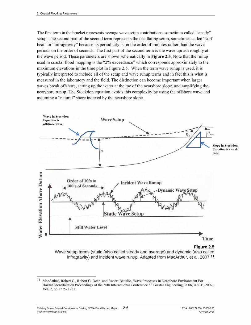
The first term in the bracket represents average wave setup contributions, sometimes called “steady”
setup. The second part of the second term represents the oscillating setup, sometimes called “surf
beat” or “infragravity” because its periodicity is on the order of minutes rather than the wave
periods on the order of seconds. The first part of the second term is the wave uprush roughly at
the wave period. These parameters are shown schematically in Figure 2.5. Note that the runup
used in coastal flood mapping is the “2% exceedance” which corresponds approximately to the
maximum elevations in the time plot in Figure 2.5. When the term wave runup is used, it is
typically interpreted to include all of the setup and wave runup terms and in fact this is what is
measured in the laboratory and the field. The distinction can become important when larger
waves break offshore, setting up the water at the toe of the nearshore slope, and amplifying the
nearshore runup. The Stockdon equation avoids this complexity by using the offshore wave and
assuming a “natural” shore indexed by the nearshore slope.
Figure 2.5
Wave setup terms (static (also called steady and average) and dynamic (also called
infragravity) and incident wave runup. Adapted from MacArthur, et al, 2007.11
11 MacArthur, Robert C., Robert G. Dean and Robert Battalio, Wave Processes In Nearshore Environment For
Hazard Identification Proceedings of the 30th International Conference of Coastal Engineering, 2006, ASCE, 2007, Vol. 2, pp 1775- 1787.
Slope in Stockdon
Equation is swash
zone
Wave in Stockdon
Equation is
offshore wave
2. Coastal Flooding Parameters
Relating Future Coastal Conditions to Existing FEMA Flood Hazard Maps 2-7 ESA / 208177.03 / 150306.00
Technical Methods Manual October 2016
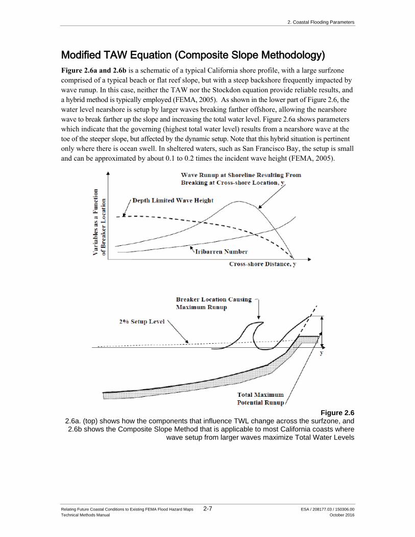
Modified TAW Equation (Composite Slope Methodology)
Figure 2.6a and 2.6b is a schematic of a typical California shore profile, with a large surfzone
comprised of a typical beach or flat reef slope, but with a steep backshore frequently impacted by
wave runup. In this case, neither the TAW nor the Stockdon equation provide reliable results, and
a hybrid method is typically employed (FEMA, 2005). As shown in the lower part of Figure 2.6, the
water level nearshore is setup by larger waves breaking farther offshore, allowing the nearshore
wave to break farther up the slope and increasing the total water level. Figure 2.6a shows parameters
which indicate that the governing (highest total water level) results from a nearshore wave at the
toe of the steeper slope, but affected by the dynamic setup. Note that this hybrid situation is pertinent
only where there is ocean swell. In sheltered waters, such as San Francisco Bay, the setup is small
and can be approximated by about 0.1 to 0.2 times the incident wave height (FEMA, 2005).
Figure 2.6
2.6a. (top) shows how the components that influence TWL change across the surfzone, and 2.6b shows the Composite Slope Method that is applicable to most California coasts where
wave setup from larger waves maximize Total Water Levels
2. Coastal Flooding Parameters
Relating Future Coastal Conditions to Existing FEMA Flood Hazard Maps 2-8 ESA / 208177.03 / 150306.00
Technical Methods Manual October 2016
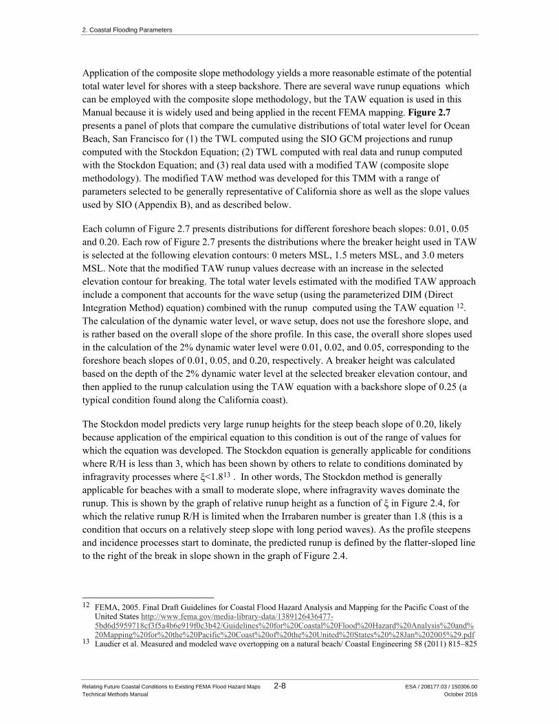
Application of the composite slope methodology yields a more reasonable estimate of the potential
total water level for shores with a steep backshore. There are several wave runup equations which
can be employed with the composite slope methodology, but the TAW equation is used in this
Manual because it is widely used and being applied in the recent FEMA mapping. Figure 2.7
presents a panel of plots that compare the cumulative distributions of total water level for Ocean
Beach, San Francisco for (1) the TWL computed using the SIO GCM projections and runup
computed with the Stockdon Equation; (2) TWL computed with real data and runup computed
with the Stockdon Equation; and (3) real data used with a modified TAW (composite slope
methodology). The modified TAW method was developed for this TMM with a range of
parameters selected to be generally representative of California shore as well as the slope values
used by SIO (Appendix B), and as described below.
Each column of Figure 2.7 presents distributions for different foreshore beach slopes: 0.01, 0.05
and 0.20. Each row of Figure 2.7 presents the distributions where the breaker height used in TAW
is selected at the following elevation contours: 0 meters MSL, 1.5 meters MSL, and 3.0 meters
MSL. Note that the modified TAW runup values decrease with an increase in the selected
elevation contour for breaking. The total water levels estimated with the modified TAW approach
include a component that accounts for the wave setup (using the parameterized DIM (Direct
Integration Method) equation) combined with the runup computed using the TAW equation 12.
The calculation of the dynamic water level, or wave setup, does not use the foreshore slope, and
is rather based on the overall slope of the shore profile. In this case, the overall shore slopes used
in the calculation of the 2% dynamic water level were 0.01, 0.02, and 0.05, corresponding to the
foreshore beach slopes of 0.01, 0.05, and 0.20, respectively. A breaker height was calculated
based on the depth of the 2% dynamic water level at the selected breaker elevation contour, and
then applied to the runup calculation using the TAW equation with a backshore slope of 0.25 (a
typical condition found along the California coast).
The Stockdon model predicts very large runup heights for the steep beach slope of 0.20, likely
because application of the empirical equation to this condition is out of the range of values for
which the equation was developed. The Stockdon equation is generally applicable for conditions
where R/H is less than 3, which has been shown by others to relate to conditions dominated by
infragravity processes where ξ<1.813 . In other words, The Stockdon method is generally
applicable for beaches with a small to moderate slope, where infragravity waves dominate the
runup. This is shown by the graph of relative runup height as a function of ξ in Figure 2.4, for
which the relative runup R/H is limited when the Irrabaren number is greater than 1.8 (this is a
condition that occurs on a relatively steep slope with long period waves). As the profile steepens
and incidence processes start to dominate, the predicted runup is defined by the flatter-sloped line
to the right of the break in slope shown in the graph of Figure 2.4.
12 FEMA, 2005. Final Draft Guidelines for Coastal Flood Hazard Analysis and Mapping for the Pacific Coast of the
United States http://www.fema.gov/media-library-data/1389126436477-5bd6d5959718cf3f5a4b6e919f0c3b42/Guidelines%20for%20Coastal%20Flood%20Hazard%20Analysis%20and%20Mapping%20for%20the%20Pacific%20Coast%20of%20the%20United%20States%20%28Jan%202005%29.pdf
13 Laudier et al. Measured and modeled wave overtopping on a natural beach/ Coastal Engineering 58 (2011) 815–825
2. Coastal Flooding Parameters
Relating Future Coastal Conditions to Existing FEMA Flood Hazard Maps 2-9 ESA / 208177.03 / 150306.00
Technical Methods Manual October 2016
Figure 2.7
Cumulative distribution of total water level at Ocean Beach, San Francisco comparing SIO GCM (green) and real data (red) calculated with the Stockdon equation and a modified TAW approach with real data (blue)
2. Coastal Flooding Parameters
Relating Future Coastal Conditions to Existing FEMA Flood Hazard Maps 2-10 ESA / 208177.03 / 150306.00
Technical Methods Manual October 2016
This page intentionally left blank
Relating Future Coastal Conditions to Existing FEMA Flood Hazard Maps 3-1 ESA / 208177.03 / 150306.00
Technical Methods Manual October 2016
CHAPTER 3
Methods to Adjust FEMA Maps for Sea Level Rise
3.1 Using FEMA Hazard Maps to Identify Future Flood Hazards Related to Sea Level Rise
This manual provides guidance to modify FEMA flood maps for future sea levels. There are
several levels of application that entail a range of effort and information. The lower levels of
application are simpler to apply and the adjustments to the future conditions hazards information
are limited. Higher levels require more effort but more accurately relate future and existing
hazards. Higher levels require more information and capability. The levels are:
1. Comparison between FEMA flood limits and future projections.
2. Adjust FEMA V-Zones to include effects of sea level rise.
3. Address other hazard zones and geomorphic processes.
4. Apply FEMA methods to SIO or other future conditions outputs.
Each of these levels is described in more detail below. Where “SIO” is stated, other sources may
be substituted (See Appendix C for other sources presently available).
Level 1: Comparison: The future conditions coastal flood values (i.e. TWL and RWL) can be
compared to the FEMA maps for a given location where both are available. The SIO values for
TWL have only been computed for six “forecast” locations using the Stockdon equation which is
comparable to FEMA TWLs for beaches. TWL levels can be selected for the range of shore
slopes that best match the conditions along the real shore. The RWLs for southern, central and
northern California (Appendix B1) can be compared to FEMA 100-year SWL elevations. The
SIO values can be selected for a range of climate scenarios (sea level rise curves) and time
horizons. Similarly, other future conditions mapping can be compared to FEMA mapping. This
approach is not recommended because of future conditions mapping by SIO (and others) use
different methods and may be biased high or low. The uncertainty range with this method is
likely to be -100% to +300% of the SIO TWL change and -20% to + 30% of the SIO RWL
change. That is, if the SIO TWL change is +2 feet, the increase to be applied to the FEMA V-
Zone elevation is somewhere in the range of +1’ to +4’ of TWL. Also, if the SIO RWL increase
is 2 feet, the increase to the FEMA A-Zone SWL is +1.6 to +2.6 feet. Other sources will deviate
more or less from the FEMA mapping, depending on the methods used (See Appendix C for
3. Technical Methods to Estimate Future Hazards
Relating Future Coastal Conditions to Existing FEMA Flood Hazard Maps 3-2 ESA / 208177.03 / 150306.00
Technical Methods Manual October 2016
sources). Better comparability will hopefully be realized in the future (see Chapter 5
Recommendations), making Level 1 Comparison more useful.
Level 2: Adjust V-Zones: Adjustment of the V-Zone for future conditions will typically be the
most useful application owing to the high hazards and insurance premiums and restrictive
building requirements associated with this zone. Depending on the data available, there are two
recommended Level 2 methodologies, identified below and described in Section 3.2:
Level 2.a: Add sea level rise: Add sea level rise to TWL and apply geomorphic adjustment and,
Level 2.b: Prorate Components: Prorate existing water level by adding future change and prorate
wave runup by multiplying by ratio of future change, and sum to get future TWL. Apply
geomorphic adjustment14.
Level 3: Address other hazard zones and geomorphic processes: Level 3 builds upon Level 2
by including modifications to A-zones, coastal erosion and coastal armoring. The Coastal A-
Zone, also known as the Limit of Moderate Wave Activity (LiMWA), is not widely used on the
Pacific coast but can be adjusted using Level 2 methods. Adjustment of coastal A-zones defined
by ponding of wave-overtopping is beyond the scope of this Manual. General guidance for
addressing coastal erosion, armoring and beach loss is provided in Section 3.3.
Level 4: Apply FEMA methods using SIO forcing parameters: The SIO outputs of flood
forcing parameters (water level and wave time series) can be substituted for the historical
conditions values used in the FEMA flood study. The flood hazards for future conditions can then
be computed and mapped. Level 3 geomorphic adjustments (e.g. coastal erosion) should also be
applied to accurately estimate future hazards. Level 4 is considered beyond the scope of this
Manual. However, Level 4 analysis has been applied in simplified test cases (BakerAECOM
2016) and in regional mapping using other future conditions projections (ESA, 2015 using GCM
output provided by the USGS CoSMoS modeling), and is being applied for southern California
at the time of this Manual.
3.2 Level 2 Adjust V-Zones
Level 2 consists of alternative methods 2a and 2b, with 2a simpler and 2b potentially more
accurate. These are described in the following two sections.
Level 2.a -Add sea level rise
The SIO future conditions projections indicate that waves and non-tidal residuals are not likely to
increase along the California coast through the rest of the 21st century and in certain areas, wave
heights may decrease slightly. Therefore, secular15 sea level rise is predicted to be the primary
14 “Geomorphic adjustment” is the change in shore geometry resulting from sea level rise, primarily due to waves
breaking on the shore at a higher elevation, and associated erosion and sediment transport. 15 Secular is used to indicate a long-term (multi-decade) trend (increase) in ocean levels, as distinguished from shorter
fluctuations.
3. Technical Methods to Estimate Future Hazards
Relating Future Coastal Conditions to Existing FEMA Flood Hazard Maps 3-3 ESA / 208177.03 / 150306.00
Technical Methods Manual October 2016
climate change driver to increase coastal flood hazards. This suggests that sea level rise could
simply be added to the total water levels (TWLs) defining the V-Zone elevations16. However, a
secular change in sea level will result in a change to the shore due to waves dissipating their
power at a higher elevation. This “morphology” response to sea level can result in a lateral shore
migration several orders of magnitude greater than the sea level rise (see also Figure 3.2).
Therefore, the following general equation is provided:
Eq (1) TWLfuture (time) = TWLexisting + SLR(time) * F(Morphology, time)
With a Morphology Function
F(Morphology, time) = 1 for erodible backshores (can use Stockdon runup equation with landward
migrated shore Figure 3.2)
F(Morphology, time) = 1 to 4, with a default of 2, for static (erosion resistant) backshores (can use
modified TAW methodology with landward overtopping extent Figure 3.4).
This formulation is similar to that developed for the FEMA Pilot Study (BakerAECOM, 2016; Vandever et
al., 2016), which uses the term Amplification Factor instead of Morphology Function.
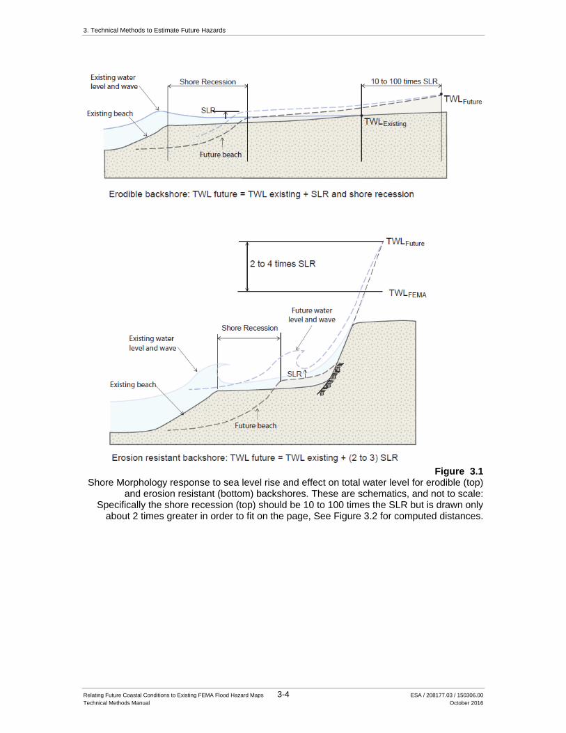
Figure 3.1 shows the effect of the morphology function schematically. The top schematic shows
an erodible shore that migrates landward in response to sea level rise, in which case the function
is 1 and the TWL increases with SLR. The bottom schematic shows an erosion-resistant
backshore, which can consist of a hard cliff or armoring, which forces the wave runup to increase
more than sea level rise by a factor of 2 to 3. Note that the Stockdon runup equation (see Chapter
2) implicitly presumes this erodible case, and therefore the landward migration of the TWL extent
needs to be computed to map the future V-Zone. The lateral component of the morphology
function is described below and graphed in Figure 3.2. The morphology function is further
described by Figure 3.4, Table 4.1 and associated text later in this section of the TMM.
The concept of shore response to sea level rise has been addressed in coastal engineering and
geomorphology practice for decades (e.g. Bruun, 1964; Everts, 1985), but remains an area of
active research and development. The implication to FEMA flood mapping has only recently
been articulated by the FEMA Pilot Study (BakerAECOM, 2016; Vandever et al, 2016) which
has influenced this Manual along with prior sea level rise studies (PWA, 2009; Revell et al, 2011;
SPUR and ESA, 2012). The TMM user should expect that new work will be published that could
augment the application of this manual.
16 This additive process is often called FEMA +1, +2 and +3 where the +1, +2 and +3 add 1, 2, or 3 feet to the existing
Flood Hazard Maps and BFEs.
3. Technical Methods to Estimate Future Hazards
Relating Future Coastal Conditions to Existing FEMA Flood Hazard Maps 3-4 ESA / 208177.03 / 150306.00
Technical Methods Manual October 2016
Figure 3.1
Shore Morphology response to sea level rise and effect on total water level for erodible (top) and erosion resistant (bottom) backshores. These are schematics, and not to scale:
Specifically the shore recession (top) should be 10 to 100 times the SLR but is drawn only about 2 times greater in order to fit on the page, See Figure 3.2 for computed distances.
3. Technical Methods to Estimate Future Hazards
Relating Future Coastal Conditions to Existing FEMA Flood Hazard Maps 3-5 ESA / 208177.03 / 150306.00
Technical Methods Manual October 2016
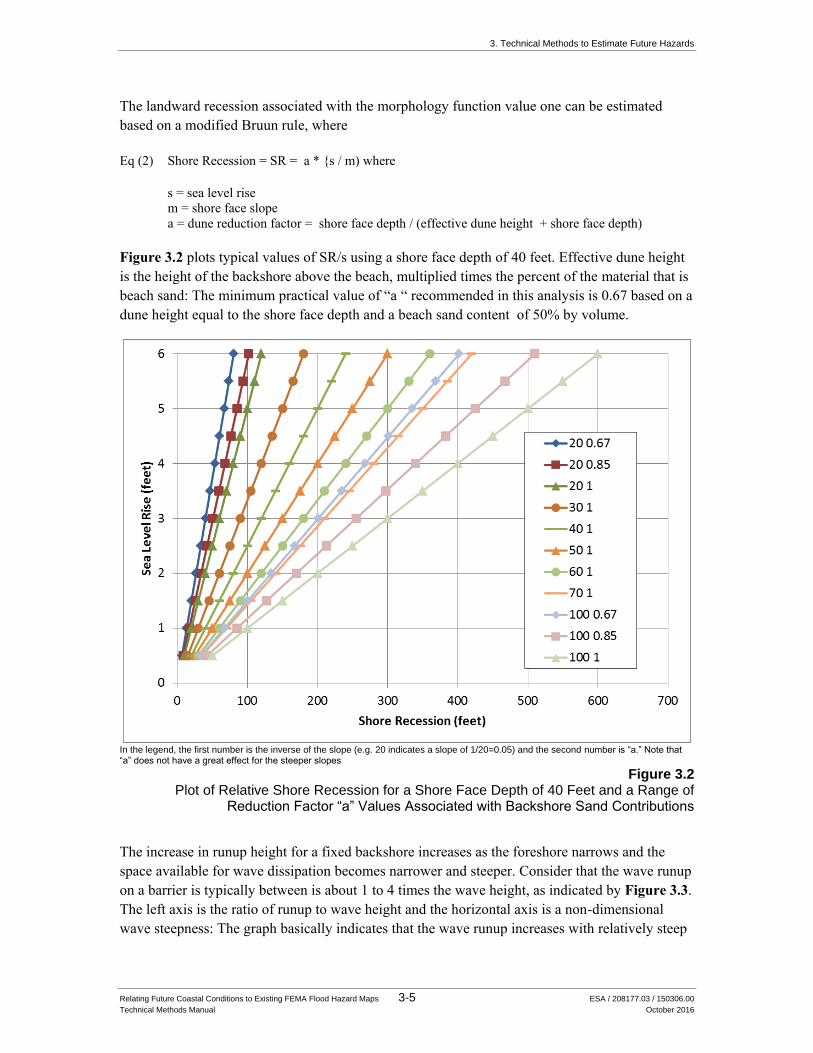
The landward recession associated with the morphology function value one can be estimated
based on a modified Bruun rule, where
Eq (2) Shore Recession = SR = a * {s / m) where
s = sea level rise
m = shore face slope
a = dune reduction factor = shore face depth / (effective dune height + shore face depth)
Figure 3.2 plots typical values of SR/s using a shore face depth of 40 feet. Effective dune height
is the height of the backshore above the beach, multiplied times the percent of the material that is
beach sand: The minimum practical value of “a “ recommended in this analysis is 0.67 based on a
dune height equal to the shore face depth and a beach sand content of 50% by volume.
In the legend, the first number is the inverse of the slope (e.g. 20 indicates a slope of 1/20=0.05) and the second number is “a.” Note that “a” does not have a great effect for the steeper slopes
Figure 3.2 Plot of Relative Shore Recession for a Shore Face Depth of 40 Feet and a Range of
Reduction Factor “a” Values Associated with Backshore Sand Contributions
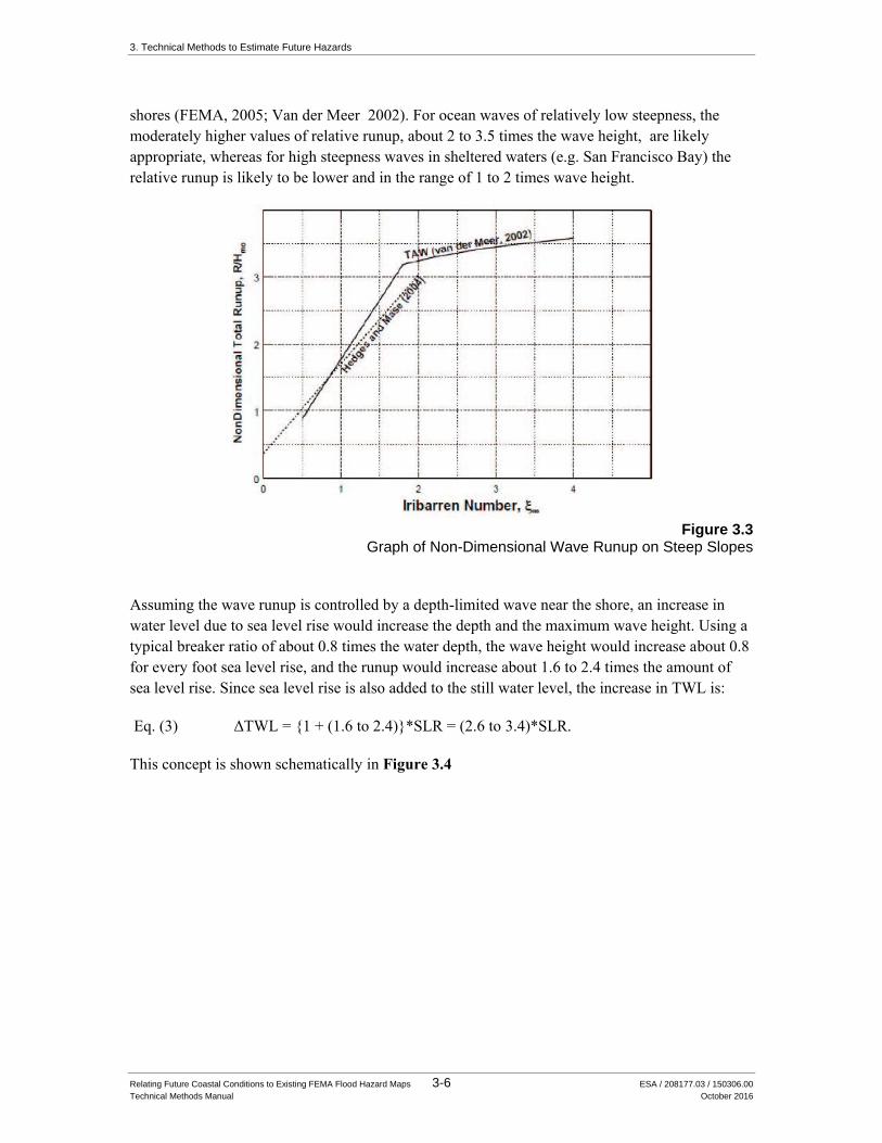
The increase in runup height for a fixed backshore increases as the foreshore narrows and the
space available for wave dissipation becomes narrower and steeper. Consider that the wave runup
on a barrier is typically between is about 1 to 4 times the wave height, as indicated by Figure 3.3.
The left axis is the ratio of runup to wave height and the horizontal axis is a non-dimensional
wave steepness: The graph basically indicates that the wave runup increases with relatively steep
3. Technical Methods to Estimate Future Hazards
Relating Future Coastal Conditions to Existing FEMA Flood Hazard Maps 3-6 ESA / 208177.03 / 150306.00
Technical Methods Manual October 2016
shores (FEMA, 2005; Van der Meer 2002). For ocean waves of relatively low steepness, the
moderately higher values of relative runup, about 2 to 3.5 times the wave height, are likely
appropriate, whereas for high steepness waves in sheltered waters (e.g. San Francisco Bay) the
relative runup is likely to be lower and in the range of 1 to 2 times wave height.
Figure 3.3
Graph of Non-Dimensional Wave Runup on Steep Slopes
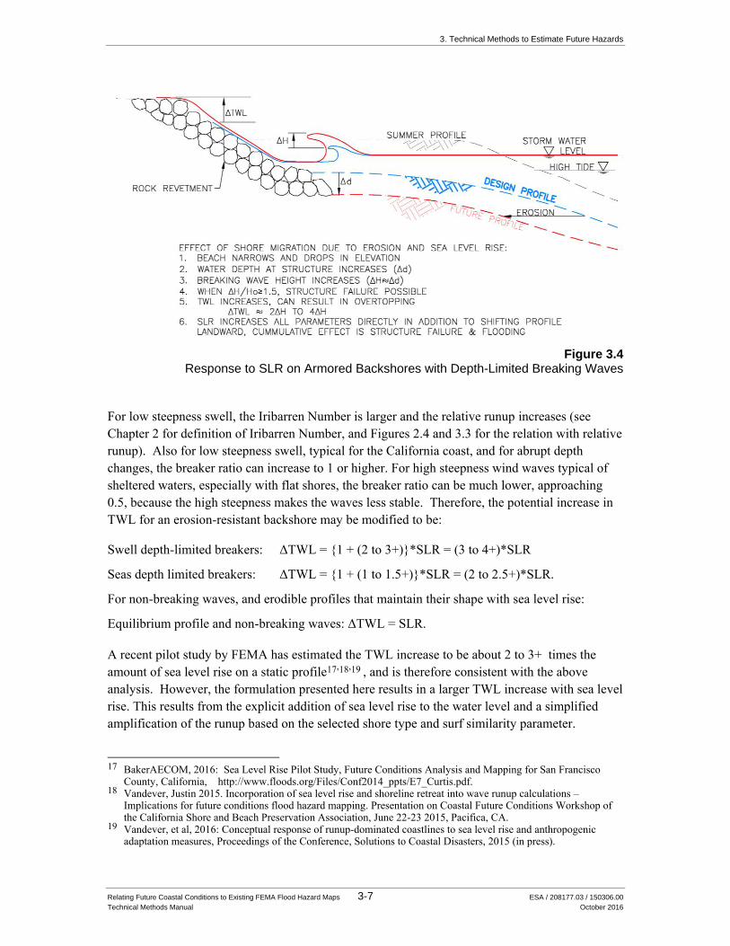
Assuming the wave runup is controlled by a depth-limited wave near the shore, an increase in
water level due to sea level rise would increase the depth and the maximum wave height. Using a
typical breaker ratio of about 0.8 times the water depth, the wave height would increase about 0.8
for every foot sea level rise, and the runup would increase about 1.6 to 2.4 times the amount of
sea level rise. Since sea level rise is also added to the still water level, the increase in TWL is:
Eq. (3) ΔTWL = {1 + (1.6 to 2.4)}*SLR = (2.6 to 3.4)*SLR.
This concept is shown schematically in Figure 3.4
3. Technical Methods to Estimate Future Hazards
Relating Future Coastal Conditions to Existing FEMA Flood Hazard Maps 3-7 ESA / 208177.03 / 150306.00
Technical Methods Manual October 2016
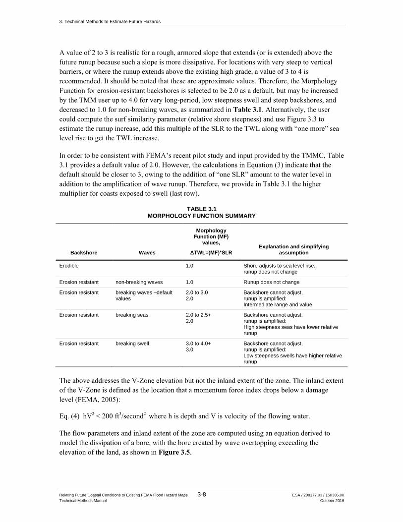
Figure 3.4
Response to SLR on Armored Backshores with Depth-Limited Breaking Waves
For low steepness swell, the Iribarren Number is larger and the relative runup increases (see
Chapter 2 for definition of Iribarren Number, and Figures 2.4 and 3.3 for the relation with relative
runup). Also for low steepness swell, typical for the California coast, and for abrupt depth
changes, the breaker ratio can increase to 1 or higher. For high steepness wind waves typical of
sheltered waters, especially with flat shores, the breaker ratio can be much lower, approaching
0.5, because the high steepness makes the waves less stable. Therefore, the potential increase in
TWL for an erosion-resistant backshore may be modified to be:
Swell depth-limited breakers: ΔTWL = {1 + (2 to 3+)}*SLR = (3 to 4+)*SLR
Seas depth limited breakers: ΔTWL = {1 + (1 to 1.5+)}*SLR = (2 to 2.5+)*SLR.
For non-breaking waves, and erodible profiles that maintain their shape with sea level rise:
Equilibrium profile and non-breaking waves: ΔTWL = SLR.
A recent pilot study by FEMA has estimated the TWL increase to be about 2 to 3+ times the
amount of sea level rise on a static profile17,18,19 , and is therefore consistent with the above
analysis. However, the formulation presented here results in a larger TWL increase with sea level
rise. This results from the explicit addition of sea level rise to the water level and a simplified
amplification of the runup based on the selected shore type and surf similarity parameter.
17 BakerAECOM, 2016: Sea Level Rise Pilot Study, Future Conditions Analysis and Mapping for San Francisco
County, California, http://www.floods.org/Files/Conf2014_ppts/E7_Curtis.pdf. 18 Vandever, Justin 2015. Incorporation of sea level rise and shoreline retreat into wave runup calculations –
Implications for future conditions flood hazard mapping. Presentation on Coastal Future Conditions Workshop of the California Shore and Beach Preservation Association, June 22-23 2015, Pacifica, CA.
19 Vandever, et al, 2016: Conceptual response of runup-dominated coastlines to sea level rise and anthropogenic adaptation measures, Proceedings of the Conference, Solutions to Coastal Disasters, 2015 (in press).
3. Technical Methods to Estimate Future Hazards
Relating Future Coastal Conditions to Existing FEMA Flood Hazard Maps 3-8 ESA / 208177.03 / 150306.00
Technical Methods Manual October 2016
A value of 2 to 3 is realistic for a rough, armored slope that extends (or is extended) above the
future runup because such a slope is more dissipative. For locations with very steep to vertical
barriers, or where the runup extends above the existing high grade, a value of 3 to 4 is
recommended. It should be noted that these are approximate values. Therefore, the Morphology
Function for erosion-resistant backshores is selected to be 2.0 as a default, but may be increased
by the TMM user up to 4.0 for very long-period, low steepness swell and steep backshores, and
decreased to 1.0 for non-breaking waves, as summarized in Table 3.1. Alternatively, the user
could compute the surf similarity parameter (relative shore steepness) and use Figure 3.3 to
estimate the runup increase, add this multiple of the SLR to the TWL along with “one more” sea
level rise to get the TWL increase.
In order to be consistent with FEMA’s recent pilot study and input provided by the TMMC, Table
3.1 provides a default value of 2.0. However, the calculations in Equation (3) indicate that the
default should be closer to 3, owing to the addition of “one SLR” amount to the water level in
addition to the amplification of wave runup. Therefore, we provide in Table 3.1 the higher
multiplier for coasts exposed to swell (last row).
TABLE 3.1 MORPHOLOGY FUNCTION SUMMARY
Backshore Waves
Morphology Function (MF)
values,
ΔTWL=(MF)*SLR Explanation and simplifying
assumption
Erodible 1.0 Shore adjusts to sea level rise, runup does not change
Erosion resistant non-breaking waves 1.0 Runup does not change
Erosion resistant breaking waves –default values
2.0 to 3.0 2.0
Backshore cannot adjust, runup is amplified: Intermediate range and value
Erosion resistant breaking seas 2.0 to 2.5+ 2.0
Backshore cannot adjust, runup is amplified: High steepness seas have lower relative runup
Erosion resistant breaking swell 3.0 to 4.0+ 3.0
Backshore cannot adjust, runup is amplified: Low steepness swells have higher relative runup
The above addresses the V-Zone elevation but not the inland extent of the zone. The inland extent
of the V-Zone is defined as the location that a momentum force index drops below a damage
level (FEMA, 2005):
Eq. (4) hV2 < 200 ft3/second2 where h is depth and V is velocity of the flowing water.
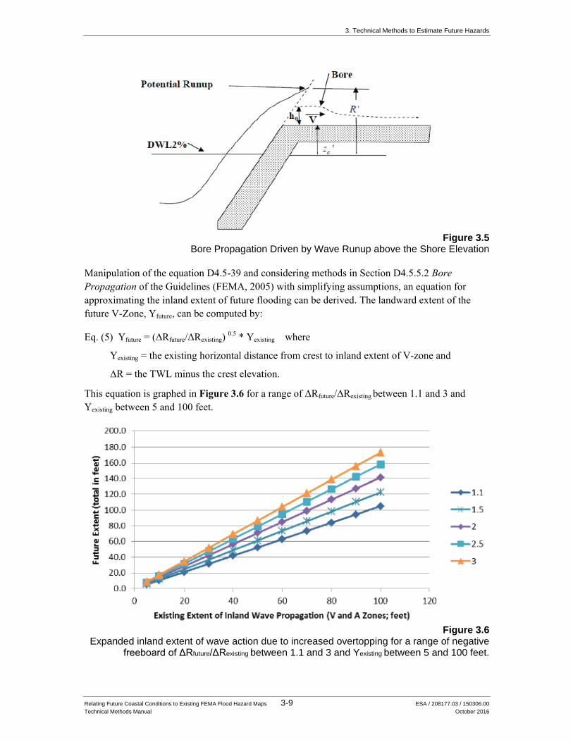
The flow parameters and inland extent of the zone are computed using an equation derived to
model the dissipation of a bore, with the bore created by wave overtopping exceeding the
elevation of the land, as shown in Figure 3.5.
3. Technical Methods to Estimate Future Hazards
Relating Future Coastal Conditions to Existing FEMA Flood Hazard Maps 3-9 ESA / 208177.03 / 150306.00
Technical Methods Manual October 2016
Figure 3.5
Bore Propagation Driven by Wave Runup above the Shore Elevation
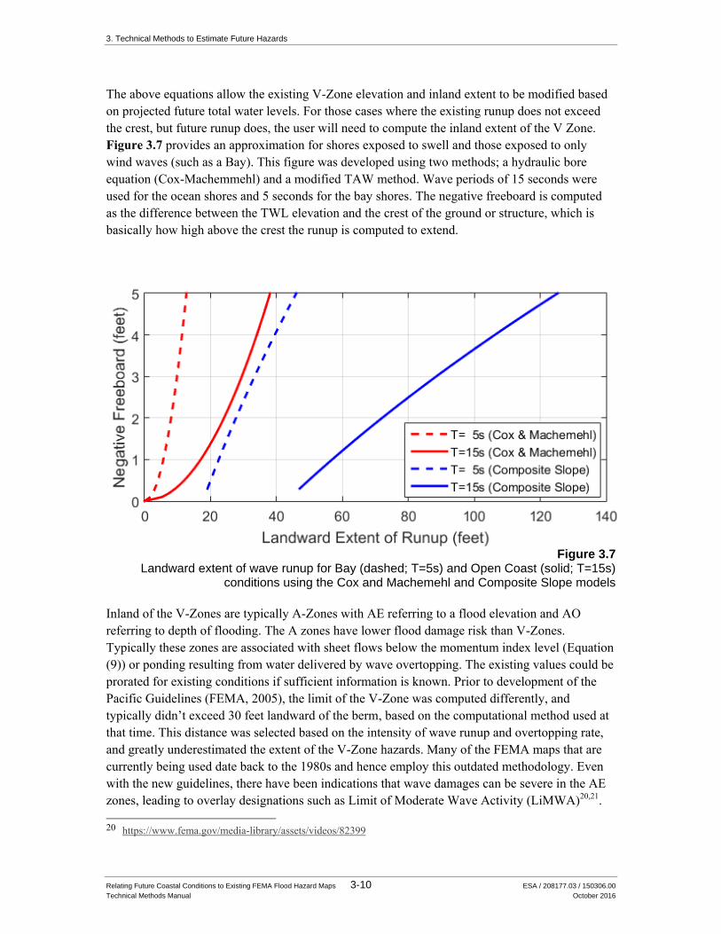
Manipulation of the equation D4.5-39 and considering methods in Section D4.5.5.2 Bore
Propagation of the Guidelines (FEMA, 2005) with simplifying assumptions, an equation for
approximating the inland extent of future flooding can be derived. The landward extent of the
future V-Zone, Yfuture, can be computed by:
Eq. (5) Yfuture = (ΔRfuture/ΔRexisting) 0.5 * Yexisting where
Yexisting = the existing horizontal distance from crest to inland extent of V-zone and
ΔR = the TWL minus the crest elevation.
This equation is graphed in Figure 3.6 for a range of ΔRfuture/ΔRexisting between 1.1 and 3 and
Yexisting between 5 and 100 feet.
Figure 3.6
Expanded inland extent of wave action due to increased overtopping for a range of negative freeboard of ΔRfuture/ΔRexisting between 1.1 and 3 and Yexisting between 5 and 100 feet.
3. Technical Methods to Estimate Future Hazards
Relating Future Coastal Conditions to Existing FEMA Flood Hazard Maps 3-10 ESA / 208177.03 / 150306.00
Technical Methods Manual October 2016
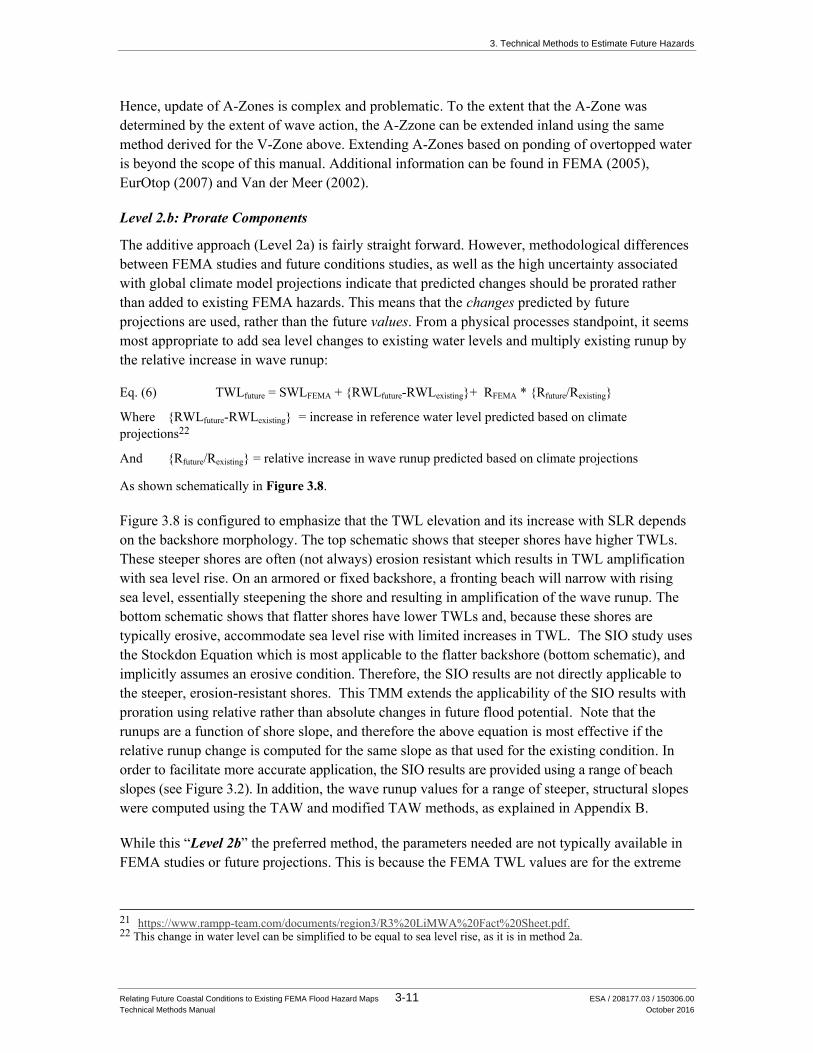
The above equations allow the existing V-Zone elevation and inland extent to be modified based
on projected future total water levels. For those cases where the existing runup does not exceed
the crest, but future runup does, the user will need to compute the inland extent of the V Zone.
Figure 3.7 provides an approximation for shores exposed to swell and those exposed to only
wind waves (such as a Bay). This figure was developed using two methods; a hydraulic bore
equation (Cox-Machemmehl) and a modified TAW method. Wave periods of 15 seconds were
used for the ocean shores and 5 seconds for the bay shores. The negative freeboard is computed
as the difference between the TWL elevation and the crest of the ground or structure, which is
basically how high above the crest the runup is computed to extend.
Figure 3.7
Landward extent of wave runup for Bay (dashed; T=5s) and Open Coast (solid; T=15s) conditions using the Cox and Machemehl and Composite Slope models
Inland of the V-Zones are typically A-Zones with AE referring to a flood elevation and AO
referring to depth of flooding. The A zones have lower flood damage risk than V-Zones.
Typically these zones are associated with sheet flows below the momentum index level (Equation
(9)) or ponding resulting from water delivered by wave overtopping. The existing values could be
prorated for existing conditions if sufficient information is known. Prior to development of the
Pacific Guidelines (FEMA, 2005), the limit of the V-Zone was computed differently, and
typically didn’t exceed 30 feet landward of the berm, based on the computational method used at
that time. This distance was selected based on the intensity of wave runup and overtopping rate,
and greatly underestimated the extent of the V-Zone hazards. Many of the FEMA maps that are
currently being used date back to the 1980s and hence employ this outdated methodology. Even
with the new guidelines, there have been indications that wave damages can be severe in the AE
zones, leading to overlay designations such as Limit of Moderate Wave Activity (LiMWA)20,21.
20 https://www.fema.gov/media-library/assets/videos/82399
3. Technical Methods to Estimate Future Hazards
Relating Future Coastal Conditions to Existing FEMA Flood Hazard Maps 3-11 ESA / 208177.03 / 150306.00
Technical Methods Manual October 2016
Hence, update of A-Zones is complex and problematic. To the extent that the A-Zone was
determined by the extent of wave action, the A-Zzone can be extended inland using the same
method derived for the V-Zone above. Extending A-Zones based on ponding of overtopped water
is beyond the scope of this manual. Additional information can be found in FEMA (2005),
EurOtop (2007) and Van der Meer (2002).
Level 2.b: Prorate Components
The additive approach (Level 2a) is fairly straight forward. However, methodological differences
between FEMA studies and future conditions studies, as well as the high uncertainty associated
with global climate model projections indicate that predicted changes should be prorated rather
than added to existing FEMA hazards. This means that the changes predicted by future
projections are used, rather than the future values. From a physical processes standpoint, it seems
most appropriate to add sea level changes to existing water levels and multiply existing runup by
the relative increase in wave runup:
Eq. (6) TWLfuture = SWLFEMA + {RWLfuture-RWLexisting}+ RFEMA * {Rfuture/Rexisting}
Where {RWLfuture-RWLexisting} = increase in reference water level predicted based on climate
projections22
And {Rfuture/Rexisting} = relative increase in wave runup predicted based on climate projections
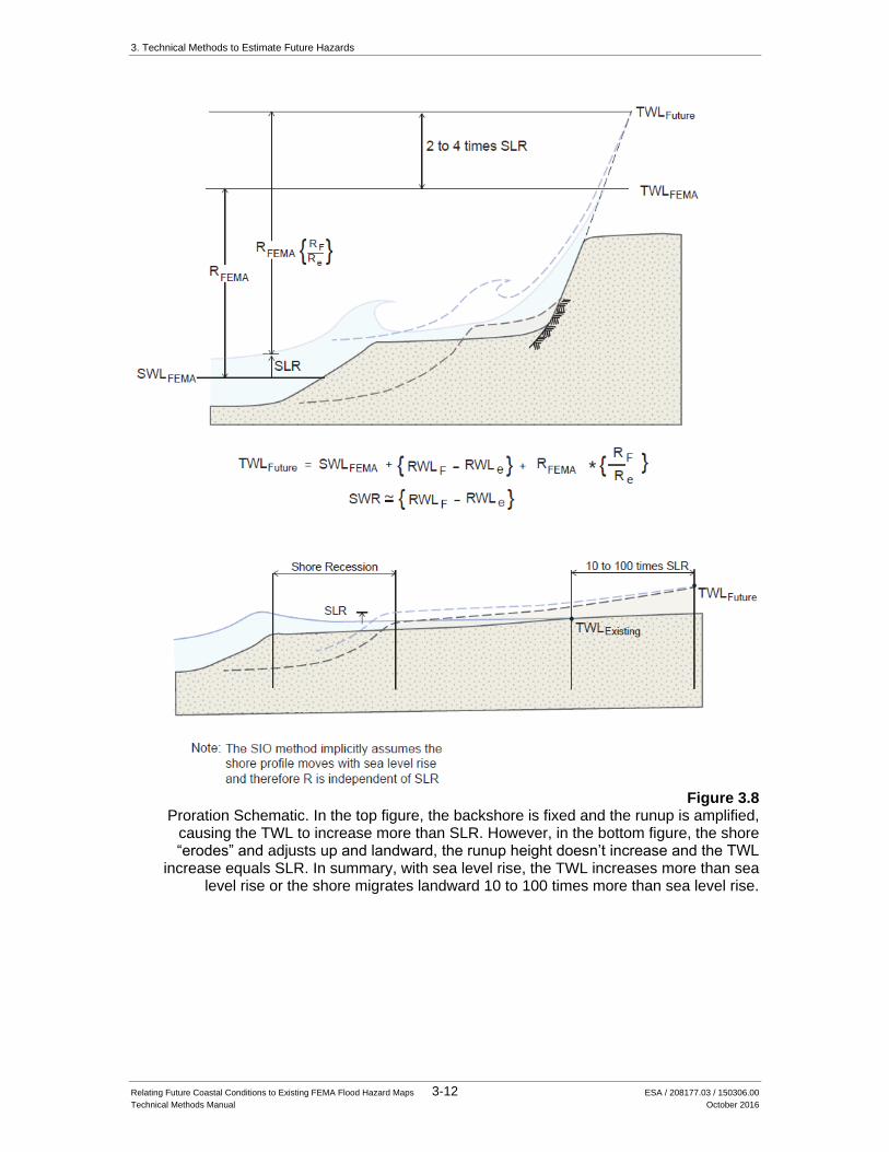
As shown schematically in Figure 3.8.
Figure 3.8 is configured to emphasize that the TWL elevation and its increase with SLR depends
on the backshore morphology. The top schematic shows that steeper shores have higher TWLs.
These steeper shores are often (not always) erosion resistant which results in TWL amplification
with sea level rise. On an armored or fixed backshore, a fronting beach will narrow with rising
sea level, essentially steepening the shore and resulting in amplification of the wave runup. The
bottom schematic shows that flatter shores have lower TWLs and, because these shores are
typically erosive, accommodate sea level rise with limited increases in TWL. The SIO study uses
the Stockdon Equation which is most applicable to the flatter backshore (bottom schematic), and
implicitly assumes an erosive condition. Therefore, the SIO results are not directly applicable to
the steeper, erosion-resistant shores. This TMM extends the applicability of the SIO results with
proration using relative rather than absolute changes in future flood potential. Note that the
runups are a function of shore slope, and therefore the above equation is most effective if the
relative runup change is computed for the same slope as that used for the existing condition. In
order to facilitate more accurate application, the SIO results are provided using a range of beach
slopes (see Figure 3.2). In addition, the wave runup values for a range of steeper, structural slopes
were computed using the TAW and modified TAW methods, as explained in Appendix B.
While this “Level 2b” the preferred method, the parameters needed are not typically available in
FEMA studies or future projections. This is because the FEMA TWL values are for the extreme
21 https://www.rampp-team.com/documents/region3/R3%20LiMWA%20Fact%20Sheet.pdf. 22 This change in water level can be simplified to be equal to sea level rise, as it is in method 2a.
3. Technical Methods to Estimate Future Hazards
Relating Future Coastal Conditions to Existing FEMA Flood Hazard Maps 3-12 ESA / 208177.03 / 150306.00
Technical Methods Manual October 2016
Figure 3.8
Proration Schematic. In the top figure, the backshore is fixed and the runup is amplified, causing the TWL to increase more than SLR. However, in the bottom figure, the shore “erodes” and adjusts up and landward, the runup height doesn’t increase and the TWL
increase equals SLR. In summary, with sea level rise, the TWL increases more than sea level rise or the shore migrates landward 10 to 100 times more than sea level rise.
3. Technical Methods to Estimate Future Hazards
Relating Future Coastal Conditions to Existing FEMA Flood Hazard Maps 3-13 ESA / 208177.03 / 150306.00
Technical Methods Manual October 2016
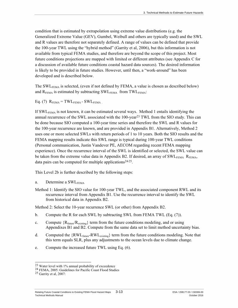
condition that is estimated by extrapolation using extreme value distributions (e.g. the
Generalized Extreme Value (GEV), Gumbel, Weibull and others are typically used) and the SWL
and R values are therefore not separately defined. A range of values can be defined that provide
the 100-year TWL using the “hybrid method” (Garrity et al, 2006), but this information is not
available from typical FEMA studies, and therefore are beyond the scope of this project. Most
future conditions projections are mapped with limited or different attributes (see Appendix C for
a discussion of available future conditions coastal hazard data sources). The desired information
is likely to be provided in future studies. However, until then, a “work-around” has been
developed and is described below.
The SWLFEMA is selected, (even if not defined by FEMA, a value is chosen as described below)
and RFEMA is estimated by subtracting SWLFEMA from TWLFEMA:
Eq. (7) RFEMA = TWLFEMA - SWLFEMA .
If SWLFEMA is not known, it can be estimated several ways. Method 1 entails identifying the
annual recurrence of the SWL associated with the 100-year23 TWL from the SIO study. This can
be done because SIO computed a 100-year time series and therefore the SWL and R values for
the 100-year recurrence are known, and are provided in Appendix B1. Alternatively, Method 2
uses one or more selected SWLs with return periods of 1 to 10 years. Both the SIO results and the
FEMA mapping results indicate this SWL range is typical during 100-year TWL conditions
(Personal communication, Justin Vandever PE, AECOM regarding recent FEMA mapping
experience). Once the recurrence interval of the SWL is identified or selected, the SWL value can
be taken from the extreme value data in Appendix B2. If desired, an array of SWLFEMA RFEMA,
data pairs can be computed for multiple applications24,25.
This Level 2b is further described by the following steps:
a. Determine a SWLFEMA
Method 1: Identify the SIO value for 100-year TWL, and the associated component RWL and its
recurrence interval from Appendix B1. Use the recurrence interval to identify the SWL
from historical data in Appendix B2.
Method 2: Select the 10-year recurrence SWL (or other) from Appendix B2.
b. Compute the R for each SWL by subtracting SWL from FEMA TWL (Eq. (7)).
c. Compute {Rfuture/Rexisting} term from the future conditions modeling, and or using
Appendixes B1 and B2. Compute from the same data set to limit method uncertainty bias.
d. Computed the {RWLfuture-RWLexisting} term from the future conditions modeling. Note that
this term equals SLR, plus any adjustments to the ocean levels due to climate change.
e. Compute the increased future TWL using Eq. (6).
23 Water level with 1% annual probability of exceedence 24 FEMA, 2005: Guidelines for Pacific Coast Flood Studies 25 Garrity et al, 2007:
3. Technical Methods to Estimate Future Hazards
Relating Future Coastal Conditions to Existing FEMA Flood Hazard Maps 3-14 ESA / 208177.03 / 150306.00
Technical Methods Manual October 2016
3.3 Considering Geomorphic Change
Geomorphic changes refer the change in land form caused by flowing water and associated
processes. The primary geomorphic processes pertinent to future conditions coastal hazard
mapping are:
Coastal erosion: long term net movement of shore location in the landward direction;
Accelerated coastal erosion: increased shore movement rate due to accelerated sea level
rise; and,
Storm-induced erosion, also called “Event Based Erosion”.
Long term erosion and accelerated erosion due to sea level rise are not included in FEMA maps.
Storm-induced, event based erosion can be included in FEMA maps based on the presumption
that the 100-year event will cause some erosion that is pertinent to the limit of coastal flood
hazards (FEMA, 2005).
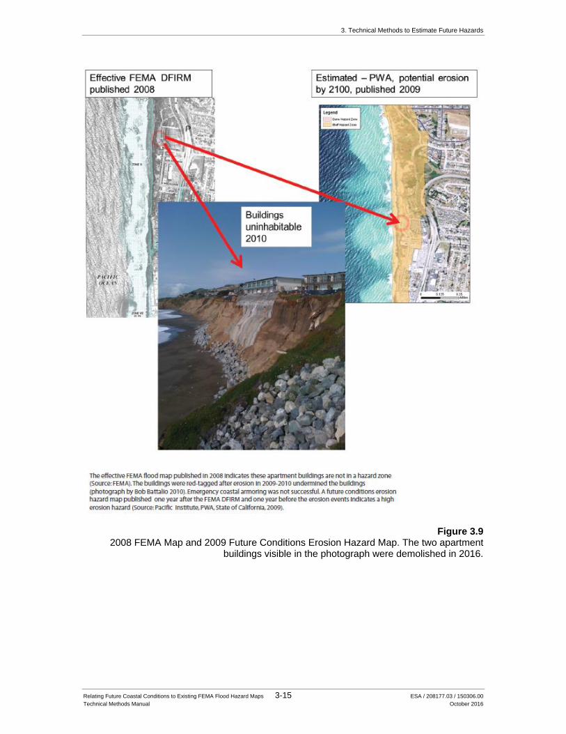
The folly of not including coastal erosion is illustrated in Figure 3.9 where the existing effective
FEMA map indicates no hazards where erosion undermined buildings and future conditions
modeling showed extensive erosion was likely.
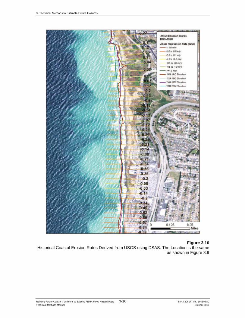
Approximate coastal erosion hazard zones can be mapped simply using available
information26,27. Figure 3.10 shows historical coastal erosion rates for the same area mapped in
Figure 3.9. These rates can be multiplied by time to determine the erosion distance to be mapped.
The use of historical erosion rates to project future shoreline position is an approximate but fairly
common means of estimating future erosion, even though erosion rates are not steady through
time28.
26 Hapke, C. and Reid, D. 2006. The National Assessment of Shoreline Change: A GIS compilation of vector
shorelines and associated shoreline change data for the sandy shorelines of the California Coast. U.S. Geological Survey. USGS Open-File report 2006-1251.
27 Hapke, C., Reid, D., and Borrelli, M. 2007. The National Assessment of Shoreline Change: A GIS compilation of vector cliff edges and associated cliff erosion data for the California Coast. U.S. Geological Survey. USGS Open-File report 2007-1112.
28 Battalio, R. T., “Littoral processes along the Pacific and bay shores of San Francisco, California, USA”, Shore & Beach, Vol. 82, No. 1, Winter 2014, pages 3-21.
3. Technical Methods to Estimate Future Hazards
Relating Future Coastal Conditions to Existing FEMA Flood Hazard Maps 3-15 ESA / 208177.03 / 150306.00
Technical Methods Manual October 2016
Figure 3.9 2008 FEMA Map and 2009 Future Conditions Erosion Hazard Map. The two apartment
buildings visible in the photograph were demolished in 2016.
3. Technical Methods to Estimate Future Hazards
Relating Future Coastal Conditions to Existing FEMA Flood Hazard Maps 3-16 ESA / 208177.03 / 150306.00
Technical Methods Manual October 2016
Figure 3.10 Historical Coastal Erosion Rates Derived from USGS using DSAS. The Location is the same
as shown in Figure 3.9
3. Technical Methods to Estimate Future Hazards
Relating Future Coastal Conditions to Existing FEMA Flood Hazard Maps 3-17 ESA / 208177.03 / 150306.00
Technical Methods Manual October 2016
Coastal erosion is projected to generally accelerate with accelerating sea level rise29. The increase
in future retreat with sea level rise can be estimated using geometric methods such as the “Bruun
rule” and more involved methods based on increased wave action reaching the back shore. A
modified Bruun rule is described by Figure 3.2 for the purposes of extending the future V-Zone
for sandy shores. This method is simplified to consider only the effect of future sea level rise and
assumes historical erosion is additive without subtracting erosion due to the historic sea level rise.
An experienced user of this manual may wish to compute erosion more accurately. The effects of
sea level rise on erosion-resistant cliffs and armored backed shores are more complex and beyond
the scope of this Manual. However, future projections are available for many areas and will likely
be available for most of the California coast within the next ten years (see Appendix C Other Sea
Level Rise Hazard Mapping Studies and Sources).
For the purposes of this Manual, future erosion can be obtained from some sources as explained
in Appendix C of this report. The uncertainty in future erosion can be depicted by mapping a
range of erosion distances computed by projection of historical erosion as well as accelerated
erosion resulting from sea level rise.
Storm “event based” erosion may be included in FEMA maps. If so, the flood zones have already
been adjusted to account for this erosion. If storm erosion is missing, storm erosion can be
calculated using methods described in the FEMA Guidelines (2005), and the V and VE zones can
be translated landward a distance equal to the computed erosion distance. Storm erosion distances
can also be derived from observations of prior erosion, if available. Finally, some of the future
conditions hazards mapping sources include storm erosion distances based on hydrodynamic or
geometric models (Appendix C).
Additional guidance and information can be found in the FEMA Pilot Study (BakerAECOM, 2016)
3.4 Accounting for Coastal Armoring Structures
Many shores have structural armoring intended to protect the back shore. These structures,
typically rock revetments (boulder slopes) and seawalls, complicate future conditions modeling
and mapping. Typically, it is assumed that a well-designed and maintained coastal armoring
structure will prevent coastal erosion from extending inland. However, coastal structures do not
prevent erosion of the seaward land (typically beaches), nor prevent wave runup and overtopping.
When considering a coastal structure, the following step-wise evaluation is recommended:
1. Is the structure certified by a professional engineer to withstand the 100-year coastal event?
2. If the structure is not certified, does it appear to have the capacity to withstand the 100-year
event now and with future higher sea levels?
3. Will wave runup exceed the structure crest now and with future higher sea levels?
29 Revell, D.L., Battalio, B., Spear, B., Ruggiero, P, and Vandever, J. A Methodology for Predicting Future Coastal
Hazards due to Sea level Rise on the California Coast. Journal of Climatic Change Climatic Change (2011) B.V. 2011 109 (Suppl 1):S251–S276, DOI 10.1007/s10584-011-0315-2, 10 December 2011 # Springer Science+Business Media
3. Technical Methods to Estimate Future Hazards
Relating Future Coastal Conditions to Existing FEMA Flood Hazard Maps 3-18 ESA / 208177.03 / 150306.00
Technical Methods Manual October 2016
4. Is the shore eroding and how much will this increase wave runup and overtopping, and
increase structural loadings into the future?
If a structure is presumed to prevent erosion, the fronting beach is still likely to erode. This will
increase the extent of wave runup and overtopping, as indicated in Figure 3.4. The effect can be
approximately accounted for by increasing the elevation of runup by 1.5 to 3 times sea level rise,
and total water level 2 to 4 times sea level rise, as described previously. The lateral extent can be
extended by shifting the flood hazard zones landward in proportion to the landward migration of
the shore fronting the coastal armor. The landward shift can be computed as the projection of
historical erosion plus the effect of sea level rise on sandy shores (explained previously). If the
beach width approaches zero, the landward extent of the future V-Zone may need to extend
inland based on the increase in negative freeboard, described previously.
Relating Future Coastal Conditions to Existing FEMA Flood Hazard Maps 4-1 ESA / 208177.03 / 150306.00
Technical Methods Manual October 2016
CHAPTER 4
Examples
Examples of TMM application are provided for Levels 1, 2a and 2b in this Chapter, using the
methods described in Chapter 3 and the data provided in Appendix B. The examples are applied
using provisional FEMA maps for Ocean Beach, San Francisco. This location was selected
because it is one of the SIO forecast locations, and it is also the site of FEMA Sea Level Rise
Pilot Study (BakerAECOM, 2015) and other future conditions studies including the Ocean Beach
Master Plan accomplished by ESA (2012). Two locations were selected for the analysis, as shown
in Figures 4.1 and 4.2. These locations were selected to represent an erodible backshore (Profile
1) and an erosion-resistant backshore (Profile 2).
Section 4.1 addresses the Level 1 “Comparison” using future values projected by SIO using GCM
output, as well as projections based on historic data, using both Stockdon and modified TAW
equations. These values were taken from Appendix B1 and B2 of this TMM. The results are
summarized in Table 4.1, along with the TWL elevations computed using Level 2a.
Section 4.2 addresses the Level 2a “Adjust V Zone, Add SLR”, including application of the
Morphology Function. This example includes shore recession (Chapter 3, Figure 3.2), increased
landward extent of overtopping (Chapter 3, Figure 3.3), and extent of future overtopping where
existing overtopping is not predicted (Chapter 3, Figure 3.6).
Section 4.3 addresses the Level 2b “Adjust V Zone, Prorate Components”, and selects the RWL
using both Method 1 based on SIO projections (Appendix B) and Method 2 selecting a different
value based on historic data (Appendix B2). This example also uses a different future conditions
study (ESA, 2012) in order to test the utility of the TMM beyond the use of SIO projections, as
well as testing the simplified morphology adjustment factors associated with Level 2a. This
section includes a brief summary of the results of the Level 2a and implications.
The Level 1 and Level 2a examples use a sea-level rise amount of 3 feet, which is approximately
the mid-range “projection” for the year 2100 developed for the Pacific Coast (NRC, 2012) and
adopted by the State of California (OPC, 2013) for vulnerability and adaptation planning. These
documents recommend considering a range of values and include a high projection of about 5.3
feet by the year 2100. Also, it is possible that higher and more rapid projections may be
recommended in the future, and the use of 3 feet is not intended to imply a recommendation.
Level 2b analysis uses a sea level rise of 4.6 feet, which is consistent with the high projection for
2100 identified by the California interim guidance (OPC, 2010) at the time the example study
was conducted.
4. Examples
Relating Future Coastal Conditions to Existing FEMA Flood Hazard Maps 4-2 ESA / 208177.03 / 150306.00
Technical Methods Manual October 2016
4.1 Example of Level 1 Comparison
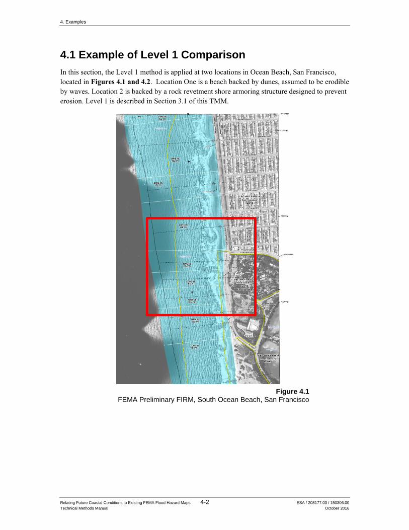
In this section, the Level 1 method is applied at two locations in Ocean Beach, San Francisco,
located in Figures 4.1 and 4.2. Location One is a beach backed by dunes, assumed to be erodible
by waves. Location 2 is backed by a rock revetment shore armoring structure designed to prevent
erosion. Level 1 is described in Section 3.1 of this TMM.
Figure 4.1 FEMA Preliminary FIRM, South Ocean Beach, San Francisco
4. Examples
Relating Future Coastal Conditions to Existing FEMA Flood Hazard Maps 4-3 ESA / 208177.03 / 150306.00
Technical Methods Manual October 2016
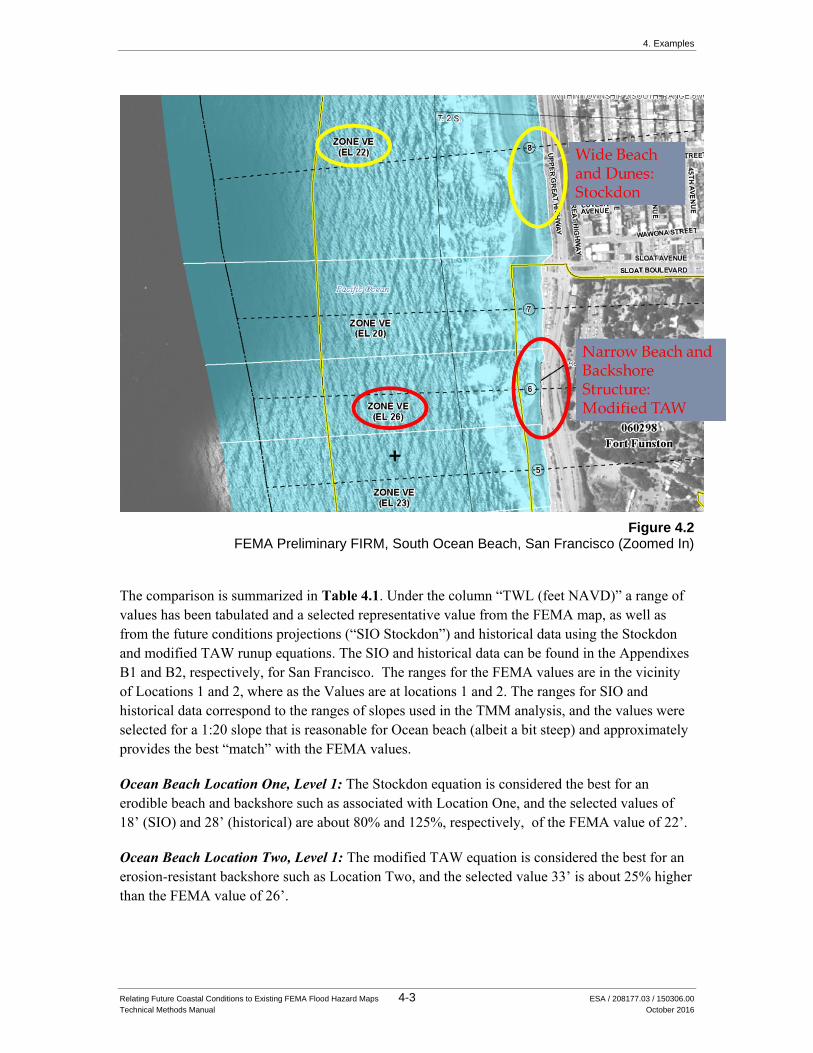
Figure 4.2 FEMA Preliminary FIRM, South Ocean Beach, San Francisco (Zoomed In)
The comparison is summarized in Table 4.1. Under the column “TWL (feet NAVD)” a range of
values has been tabulated and a selected representative value from the FEMA map, as well as
from the future conditions projections (“SIO Stockdon”) and historical data using the Stockdon
and modified TAW runup equations. The SIO and historical data can be found in the Appendixes
B1 and B2, respectively, for San Francisco. The ranges for the FEMA values are in the vicinity
of Locations 1 and 2, where as the Values are at locations 1 and 2. The ranges for SIO and
historical data correspond to the ranges of slopes used in the TMM analysis, and the values were
selected for a 1:20 slope that is reasonable for Ocean beach (albeit a bit steep) and approximately
provides the best “match” with the FEMA values.
Ocean Beach Location One, Level 1: The Stockdon equation is considered the best for an
erodible beach and backshore such as associated with Location One, and the selected values of
18’ (SIO) and 28’ (historical) are about 80% and 125%, respectively, of the FEMA value of 22’.
Ocean Beach Location Two, Level 1: The modified TAW equation is considered the best for an
erosion-resistant backshore such as Location Two, and the selected value 33’ is about 25% higher
than the FEMA value of 26’.
4. Examples
Relating Future Coastal Conditions to Existing FEMA Flood Hazard Maps 4-4 ESA / 208177.03 / 150306.00
Technical Methods Manual October 2016
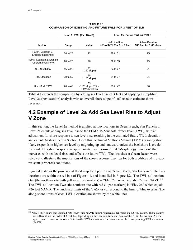
TABLE 4.1 COMPARISON OF EXISTING AND FUTURE TWLS FOR 3 FEET OF SLR
Method
Level 1: TWL (feet NAVD) Level 2a: Future TWL w/ 3' SLR
Range Value Hold the line
+(2 to 3)*SLR = 6 to 9 feet Allow Erosion
180 feet for 1:60 slope
FEMA: Location 1, Erodible backshore
16 to 23 22 28 to 31 25
FEMA: Location 2, Erosion resistant backshore
20 to 26 26 32 to 35 29
SIO Stockdon 15 to 26 18
(1:20 slope) 24 to 27 21
Hist. Stockdon 20 to 69 28
(1:20 slope) 34 to 37 31
Hist. Mod. TAW 26 to 43 33
(1:20 slope; 2.5m NAVD breaker)
39 to 42 36
Table 4.1 extends the comparison by adding sea level rise of 3 feet and applying a simplified
Level 2a (next section) analysis with an overall shore slope of 1:60 used to estimate shore
recession.
4.2 Example of Level 2a Add Sea Level Rise to Adjust V Zone
In this section, the Level 2a method is applied at two locations in Ocean Beach, San Francisco.
Level 2a entails adding sea level rise to the FEMA V-Zone total water level (TWL), with an
adjustment for shore response to sea level rise, resulting in the estimated future TWL elevation
and extent. As described in Section 3.2 of this Technical Methods Manual (TMM), a sandy shore
likely responds to higher sea level by migrating up and landward unless the backshore is erosion-
resistant. This shore response is approximated with a simplified “Morphology Function” that
increases with sea level rise, and affects the future TWL. The two sites at Ocean Beach were
selected to illustrate the implications of the shore response function for both erodible and erosion-
resistant (armored) conditions.
Figure 4.1 shows the provisional flood map for a portion of Ocean Beach, San Francisco. The two
locations are within the red box of Figure 4.1, and identified in Figure 4.2. The TWL at Location
One (the northern site with yellow ellipse markers) is “Elev 22” which equals +22 feet NAVD.30
The TWL at Location Two (the southern site with red ellipse markers) is “Elev 26” which equals
+26 feet NAVD. The landward limits of the V-Zones correspond to the limit of blue overlay. The
along-shore limits of each TWL elevation are shown by the white lines.
30 New FEMA maps and updated “DFIRMS” use NAVD datum, whereas older maps use NGVD datum. These datums
are different, on the order of 3 feet +/-, depending on the location, time and basis of the NGVD elevation. A very approximate correction is to add 3 feet to the TWL elevation NGVD to estimate the corresponding TWL elevation NAVD.
4. Examples
Relating Future Coastal Conditions to Existing FEMA Flood Hazard Maps 4-5 ESA / 208177.03 / 150306.00
Technical Methods Manual October 2016
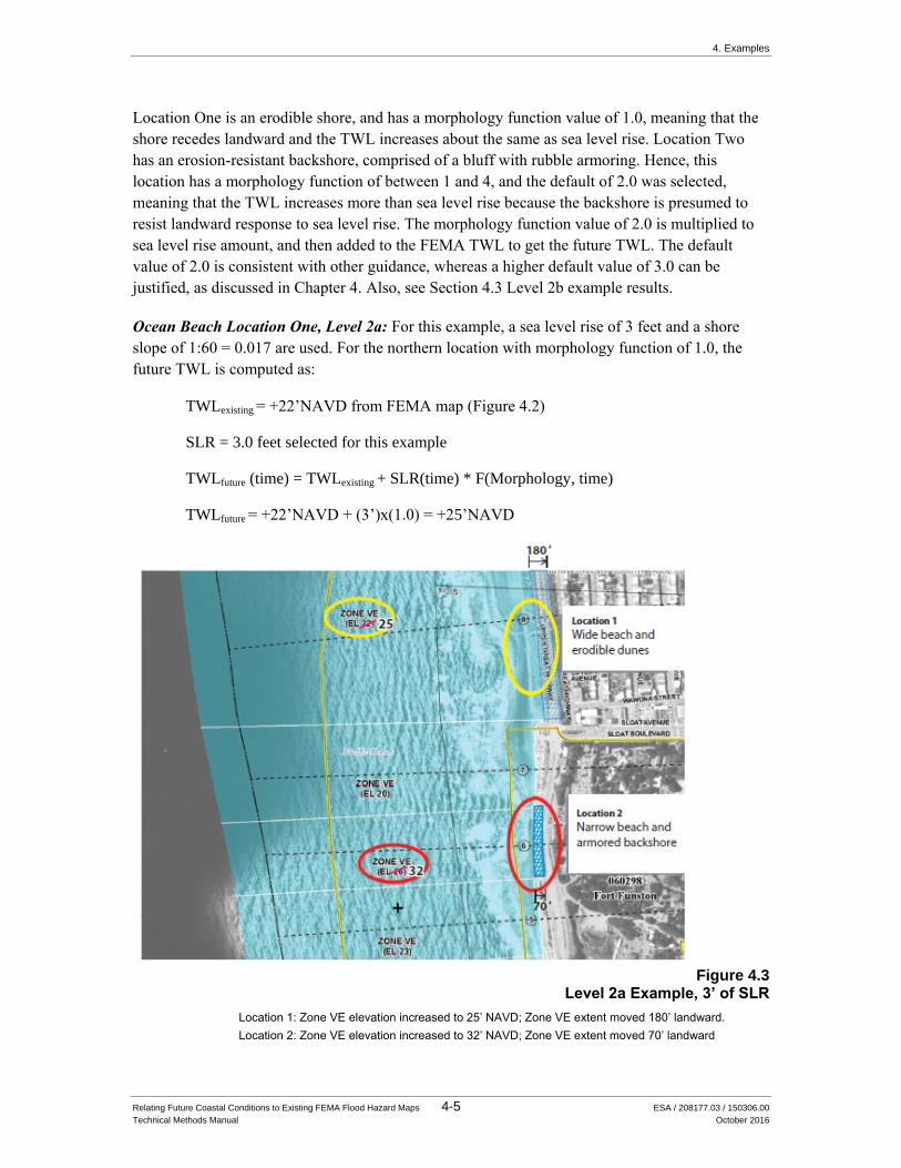
Location One is an erodible shore, and has a morphology function value of 1.0, meaning that the
shore recedes landward and the TWL increases about the same as sea level rise. Location Two
has an erosion-resistant backshore, comprised of a bluff with rubble armoring. Hence, this
location has a morphology function of between 1 and 4, and the default of 2.0 was selected,
meaning that the TWL increases more than sea level rise because the backshore is presumed to
resist landward response to sea level rise. The morphology function value of 2.0 is multiplied to
sea level rise amount, and then added to the FEMA TWL to get the future TWL. The default
value of 2.0 is consistent with other guidance, whereas a higher default value of 3.0 can be
justified, as discussed in Chapter 4. Also, see Section 4.3 Level 2b example results.
Ocean Beach Location One, Level 2a: For this example, a sea level rise of 3 feet and a shore
slope of 1:60 = 0.017 are used. For the northern location with morphology function of 1.0, the
future TWL is computed as:
TWLexisting = +22’NAVD from FEMA map (Figure 4.2)
SLR = 3.0 feet selected for this example
TWLfuture (time) = TWLexisting + SLR(time) * F(Morphology, time)
TWLfuture = +22’NAVD + (3’)x(1.0) = +25’NAVD
Figure 4.3
Level 2a Example, 3’ of SLR
Location 1: Zone VE elevation increased to 25’ NAVD; Zone VE extent moved 180’ landward.
Location 2: Zone VE elevation increased to 32’ NAVD; Zone VE extent moved 70’ landward
4. Examples
Relating Future Coastal Conditions to Existing FEMA Flood Hazard Maps 4-6 ESA / 208177.03 / 150306.00
Technical Methods Manual October 2016
Lateral backshore recession based on Figure 3.2 with a slope of 1:60 is 180 feet.. The future V-
Zone is mapped with an elevation of +25’ NAVD and extended landward 180 feet, as shown in
Figure 4.3.
Ocean Beach Location Two, Level 2a: For this example, a sea level rise of 3 feet and a shore
slope of 1:60 = 0.017 are used. For the northern location with morphology function of 2.0, the
future TWL is computed as:
TWLexisting = +26’NAVD from FEMA map (Figure 4.2)
SLR = 3.0 feet selected for this example
TWLfuture (time) = TWLexisting + SLR(time) * F(Morphology, time)
TWLfuture = +26’NAVD + (3’)x(2.0) = +32’NAVD
Backshore recession is presumed stopped by the shore armor. However, the future TWL exceeds
the top of the armored bluff by approximately 2 feet (the existing bluff top elevation is +30’
NAVD and the computed TWL is +32’ NAVD). Based on Figure 3.6 using a negative freeboard
of 2 feet, the inland extent of the TWL is computed as 22’ (Cox-Machemehl) to 70’ (composite
slope), using the 15-second ocean wave period. This example indicates the range of values (20’ to
70’) that can be generated using the information in this manual is large and indicates some of the
uncertainty inherent in future projections.
The future V-Zone is mapped with an elevation of +32’ NAVD and extended landward 70 feet, as
shown in Figure 4.3.
Note that the FEMA map does not show overtopping of the bluff top by wave runup. However,
for the purposes of illustration of the use of the TMM, let’s pretend that the FEMA map indicates
that the TWL exceeds the bluff top by one foot vertically and the V Zone limits extend 20 feet
inland of the bluff crest. With 3 feet of sea level rise, the future TWL is 6 feet higher, indicating
that the negative freeboard (TWL above crest elevation) grows from 1’ to 7’. To calculate the
future landward limit of the V Zone, Figure 3.5 could be used except the lines show only ratios up
to 3, or the equation:
Yfuture = (ΔRfuture/ΔRexisting) 0.5 * Yexisting = (7’/1’) 0.5* 20’ = 52.9’ =~50’.
The net change is calculated as:
ΔY = Yfuture - Yexisting = 50’-20’ = 30’.
This theoretical example would result in the V Zone being extended 30 feet landward. Note that
the theoretical landward extent of 20 feet for 1 foot of overtopping was selected to correspond
approximately to the Cox-Machemehl, 15 second line in Figure 3.6. However, if the Composite
Slope, 15 second line was used the landward extent would be closer to 60 feet for existing
conditions, indicating that the FEMA methodology may under-predict the landward limit of wave
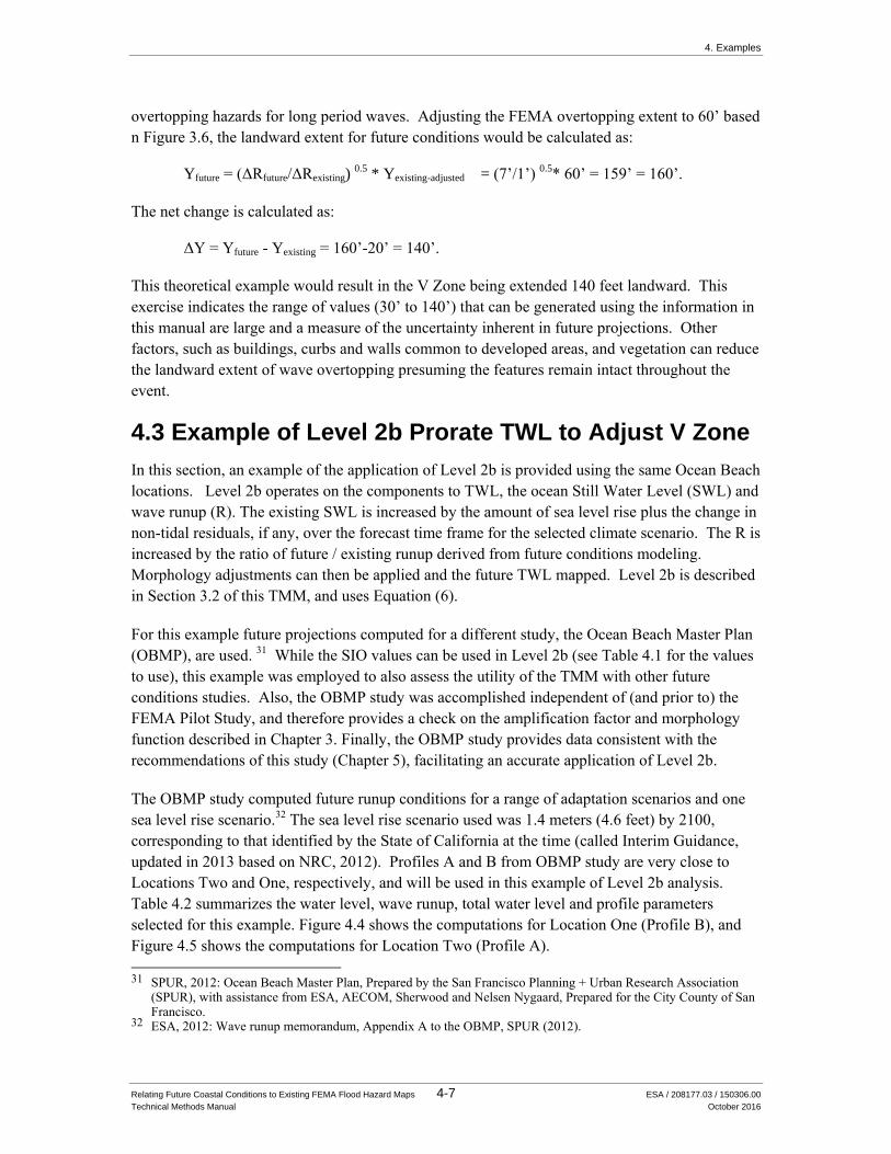
4. Examples
Relating Future Coastal Conditions to Existing FEMA Flood Hazard Maps 4-7 ESA / 208177.03 / 150306.00
Technical Methods Manual October 2016
overtopping hazards for long period waves. Adjusting the FEMA overtopping extent to 60’ based
n Figure 3.6, the landward extent for future conditions would be calculated as:
Yfuture = (ΔRfuture/ΔRexisting) 0.5 * Yexisting-adjusted = (7’/1’) 0.5* 60’ = 159’ = 160’.
The net change is calculated as:
ΔY = Yfuture - Yexisting = 160’-20’ = 140’.
This theoretical example would result in the V Zone being extended 140 feet landward. This
exercise indicates the range of values (30’ to 140’) that can be generated using the information in
this manual are large and a measure of the uncertainty inherent in future projections. Other
factors, such as buildings, curbs and walls common to developed areas, and vegetation can reduce
the landward extent of wave overtopping presuming the features remain intact throughout the
event.
4.3 Example of Level 2b Prorate TWL to Adjust V Zone
In this section, an example of the application of Level 2b is provided using the same Ocean Beach
locations. Level 2b operates on the components to TWL, the ocean Still Water Level (SWL) and
wave runup (R). The existing SWL is increased by the amount of sea level rise plus the change in
non-tidal residuals, if any, over the forecast time frame for the selected climate scenario. The R is
increased by the ratio of future / existing runup derived from future conditions modeling.
Morphology adjustments can then be applied and the future TWL mapped. Level 2b is described
in Section 3.2 of this TMM, and uses Equation (6).
For this example future projections computed for a different study, the Ocean Beach Master Plan
(OBMP), are used. 31 While the SIO values can be used in Level 2b (see Table 4.1 for the values
to use), this example was employed to also assess the utility of the TMM with other future
conditions studies. Also, the OBMP study was accomplished independent of (and prior to) the
FEMA Pilot Study, and therefore provides a check on the amplification factor and morphology
function described in Chapter 3. Finally, the OBMP study provides data consistent with the
recommendations of this study (Chapter 5), facilitating an accurate application of Level 2b.
The OBMP study computed future runup conditions for a range of adaptation scenarios and one
sea level rise scenario.32 The sea level rise scenario used was 1.4 meters (4.6 feet) by 2100,
corresponding to that identified by the State of California at the time (called Interim Guidance,
updated in 2013 based on NRC, 2012). Profiles A and B from OBMP study are very close to
Locations Two and One, respectively, and will be used in this example of Level 2b analysis.
Table 4.2 summarizes the water level, wave runup, total water level and profile parameters
selected for this example. Figure 4.4 shows the computations for Location One (Profile B), and
Figure 4.5 shows the computations for Location Two (Profile A).
31 SPUR, 2012: Ocean Beach Master Plan, Prepared by the San Francisco Planning + Urban Research Association
(SPUR), with assistance from ESA, AECOM, Sherwood and Nelsen Nygaard, Prepared for the City County of San Francisco.
32 ESA, 2012: Wave runup memorandum, Appendix A to the OBMP, SPUR (2012).
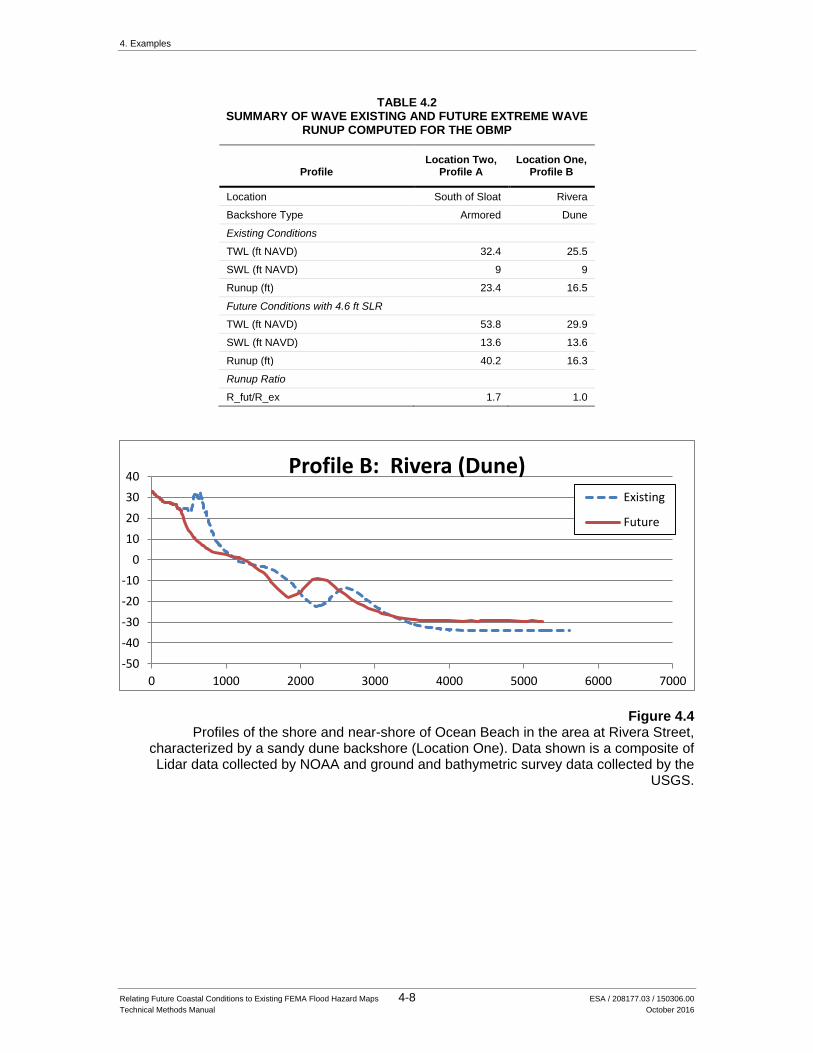
4. Examples
Relating Future Coastal Conditions to Existing FEMA Flood Hazard Maps 4-8 ESA / 208177.03 / 150306.00
Technical Methods Manual October 2016
TABLE 4.2 SUMMARY OF WAVE EXISTING AND FUTURE EXTREME WAVE
RUNUP COMPUTED FOR THE OBMP
Profile Location Two,
Profile A Location One,
Profile B
Location South of Sloat Rivera
Backshore Type Armored Dune
Existing Conditions
TWL (ft NAVD) 32.4 25.5
SWL (ft NAVD) 9 9
Runup (ft) 23.4 16.5
Future Conditions with 4.6 ft SLR
TWL (ft NAVD) 53.8 29.9
SWL (ft NAVD) 13.6 13.6
Runup (ft) 40.2 16.3
Runup Ratio
R_fut/R_ex 1.7 1.0
Figure 4.4 Profiles of the shore and near-shore of Ocean Beach in the area at Rivera Street,
characterized by a sandy dune backshore (Location One). Data shown is a composite of Lidar data collected by NOAA and ground and bathymetric survey data collected by the
USGS.
-50
-40
-30
-20
-10
0
10
20
30
40
0 1000 2000 3000 4000 5000 6000 7000
Profile B: Rivera (Dune) Existing
Future
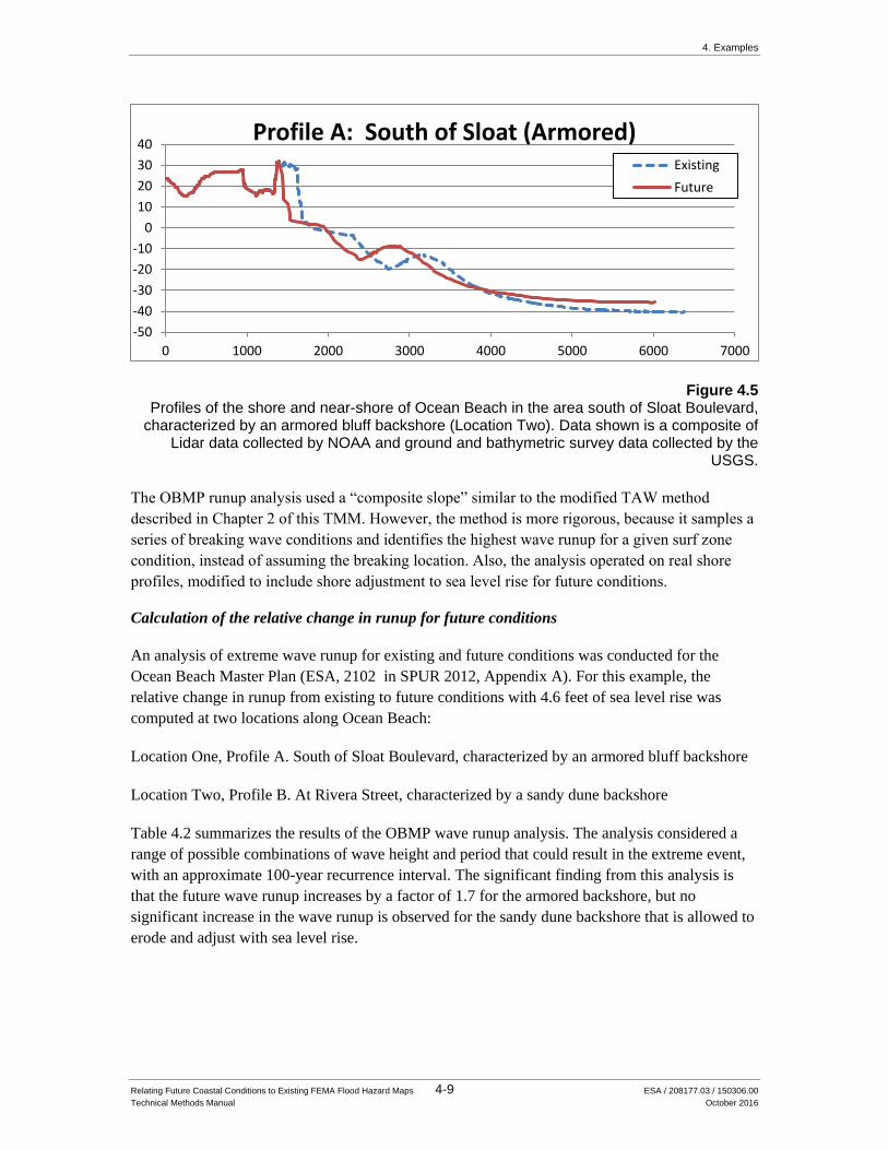
4. Examples
Relating Future Coastal Conditions to Existing FEMA Flood Hazard Maps 4-9 ESA / 208177.03 / 150306.00
Technical Methods Manual October 2016
Figure 4.5 Profiles of the shore and near-shore of Ocean Beach in the area south of Sloat Boulevard,
characterized by an armored bluff backshore (Location Two). Data shown is a composite of Lidar data collected by NOAA and ground and bathymetric survey data collected by the
USGS.
The OBMP runup analysis used a “composite slope” similar to the modified TAW method
described in Chapter 2 of this TMM. However, the method is more rigorous, because it samples a
series of breaking wave conditions and identifies the highest wave runup for a given surf zone
condition, instead of assuming the breaking location. Also, the analysis operated on real shore
profiles, modified to include shore adjustment to sea level rise for future conditions.
Calculation of the relative change in runup for future conditions
An analysis of extreme wave runup for existing and future conditions was conducted for the
Ocean Beach Master Plan (ESA, 2102 in SPUR 2012, Appendix A). For this example, the
relative change in runup from existing to future conditions with 4.6 feet of sea level rise was
computed at two locations along Ocean Beach:
Location One, Profile A. South of Sloat Boulevard, characterized by an armored bluff backshore
Location Two, Profile B. At Rivera Street, characterized by a sandy dune backshore
Table 4.2 summarizes the results of the OBMP wave runup analysis. The analysis considered a
range of possible combinations of wave height and period that could result in the extreme event,
with an approximate 100-year recurrence interval. The significant finding from this analysis is
that the future wave runup increases by a factor of 1.7 for the armored backshore, but no
significant increase in the wave runup is observed for the sandy dune backshore that is allowed to
erode and adjust with sea level rise.
-50
-40
-30
-20
-10
0
10
20
30
40
0 1000 2000 3000 4000 5000 6000 7000
Profile A: South of Sloat (Armored) Existing
Future
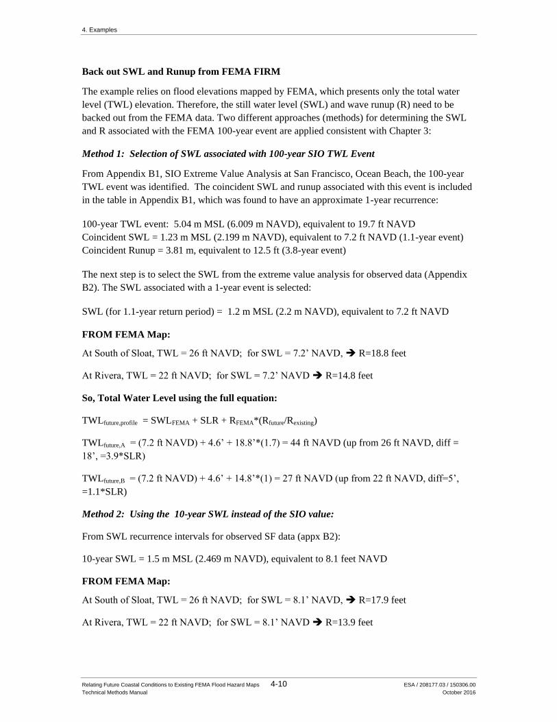
4. Examples
Relating Future Coastal Conditions to Existing FEMA Flood Hazard Maps 4-10 ESA / 208177.03 / 150306.00
Technical Methods Manual October 2016
Back out SWL and Runup from FEMA FIRM
The example relies on flood elevations mapped by FEMA, which presents only the total water
level (TWL) elevation. Therefore, the still water level (SWL) and wave runup (R) need to be
backed out from the FEMA data. Two different approaches (methods) for determining the SWL
and R associated with the FEMA 100-year event are applied consistent with Chapter 3:
Method 1: Selection of SWL associated with 100-year SIO TWL Event
From Appendix B1, SIO Extreme Value Analysis at San Francisco, Ocean Beach, the 100-year
TWL event was identified. The coincident SWL and runup associated with this event is included
in the table in Appendix B1, which was found to have an approximate 1-year recurrence:
100-year TWL event: 5.04 m MSL (6.009 m NAVD), equivalent to 19.7 ft NAVD
Coincident SWL = 1.23 m MSL (2.199 m NAVD), equivalent to 7.2 ft NAVD (1.1-year event)
Coincident Runup = 3.81 m, equivalent to 12.5 ft (3.8-year event)
The next step is to select the SWL from the extreme value analysis for observed data (Appendix
B2). The SWL associated with a 1-year event is selected:
SWL (for 1.1-year return period) = 1.2 m MSL (2.2 m NAVD), equivalent to 7.2 ft NAVD
FROM FEMA Map:
At South of Sloat, TWL = 26 ft NAVD; for SWL = 7.2’ NAVD, R=18.8 feet
At Rivera, TWL = 22 ft NAVD; for SWL = 7.2’ NAVD R=14.8 feet
So, Total Water Level using the full equation:
TWLfuture,profile = SWLFEMA + SLR + RFEMA*(Rfuture/Rexisting)
TWLfuture,A = (7.2 ft NAVD) + 4.6’ + 18.8’*(1.7) = 44 ft NAVD (up from 26 ft NAVD, diff =
18’, =3.9*SLR)
TWLfuture,B = (7.2 ft NAVD) + 4.6’ + 14.8’*(1) = 27 ft NAVD (up from 22 ft NAVD, diff=5’,
=1.1*SLR)
Method 2: Using the 10-year SWL instead of the SIO value:
From SWL recurrence intervals for observed SF data (appx B2):
10-year SWL = 1.5 m MSL (2.469 m NAVD), equivalent to 8.1 feet NAVD
FROM FEMA Map:
At South of Sloat, TWL = 26 ft NAVD; for SWL = 8.1’ NAVD, R=17.9 feet
At Rivera, TWL = 22 ft NAVD; for SWL = 8.1’ NAVD R=13.9 feet
4. Examples
Relating Future Coastal Conditions to Existing FEMA Flood Hazard Maps 4-11 ESA / 208177.03 / 150306.00
Technical Methods Manual October 2016
TWLfuture,A = (8.1 ft NAVD) + 4.6’ + 17.9’*(1.7) = 43 ft NAVD (up from 26 ft NAVD, diff =
17’, =3.7*SLR)
TWLfuture,B = (8.1 ft NAVD) + 4.6’ + 13.9’*(1) = 26.6 ft NAVD (up from 22 ft NAVD, diff=4.6’,
=1*SLR)
Results of Level 2b Example:Two methods were used: Method 1 used the SIO values to identify
the SWL recurrence probability which had about a 1-year return period, while Method 2 used a
10-year return period SWL which is reportedly more consistent with findings during the FEMA
pilot study, as described in Chapter 3 of this TMM. The differences in SWL and resulting TWL
were about one foot. Method 2 is preferred because it de-emphasizes method uncertainty
associated with the proration of runup and can be employed independently of the SIO study.
For Location One (Profile B), which is an erodible shore, the results indicated that the TWL
increased by the amount of SLR, which was 4.6 feet. For Location Two (Profile A), which has an
erosion-resistant backshore, the results indicated that TWL increased about 3.7 (Method 2 using
10-year SWL) to 3.9 (Method 1 using 1-year SWL). These results are consistent with the
morphology response function described in Chapter 3 of this TMM. Note that the wave
conditions used were for swell, consistent with higher amplification of TWL due to SLR for
erosion –resistant backshores.
The results indicate that the wave runup amplification factor may be higher than the 2-3 identified
by the FEMA pilot study. This may be due to the direct addition of slr as well as runup
amplification associated with Level 2b, which essentially increases the amplification factor by
1.0.
4. Examples
Relating Future Coastal Conditions to Existing FEMA Flood Hazard Maps 4-12 ESA / 208177.03 / 150306.00
Technical Methods Manual October 2016
This page intentionally left blank
Relating Future Coastal Conditions to Existing FEMA Flood Hazard Maps 5-1 ESA / 208177.03 / 150306.00
Technical Methods Manual October 2016
CHAPTER 5
Recommendations
1. FEMA existing conditions studies should include the still water levels (SWL) and wave
runup values (R) for each total water level (TWL) used to define high velocity zones (V
Zones). This may require additional work, to calculate and select the SWL and R values
most appropriate for the 100-year TWL. Other information, such as the shore profile
geometry, equations used, and profile parameters such as slopes should also be provided.33
2. Future conditions flood studies should provide the TWL, SWL and R values for mapped or
otherwise designated location. Other information, such as the shore profile geometry,
equations used, and profile parameters such as slopes should also be provided.
3. Both FEMA existing conditions studies and future conditions studies by FEMA or others
should provide guidance on how the study results can be related to future conditions, and
existing FEMA maps, respectively.
4. Studies should characterize the existing backshore conditions in terms of the morphology
function defined in this Technical Methods Manual. The required information consists of
whether the shore is erodible or not, and the type of wave condition driving the hazard
(breaking or not, long period swell or short period seas). Table 3.1 (repeated below as
Table 5.1) provides an overview of the Morphology Function concept and suggested
values. Note that in most cases, the total water level (TWL) increases (ΔTWL) more than
the amount of sea level rise (SLR), unless the shore adjusts landward, with the exception
being for non-breaking waves. Adaptation measures are not included in this analysis.
5. Coastal erosion should be considered in addition to flooding, along with estimates of the
increase in erosion rates with sea level rise.
6. Additional attention needs to be applied to develop specific guidance for quantifying future
coastal hazards, building upon the substantial progress made to date by California, NOAA
and others. The “gap” to be filled or bridged is between the substantial progress made by
science informing policy and educating the public, and the needs at the planning and
engineering applications level. While requiring a multi-discipline effort, greater
participation by engineers is required to develop practical solutions needed to facilitate
informed planning and resilient design.
33 During review, we were informed comparable data will be made available (personal communication, Justin
Vandever, AECOM). The report required to access this information is referred to as Intermediate Data Submittal #3 – Nearshore Hydraulics, and is produced for each County. See Appendix D for more information.
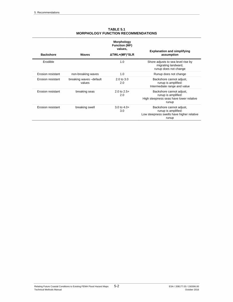
5. Recommendations
Relating Future Coastal Conditions to Existing FEMA Flood Hazard Maps 5-2 ESA / 208177.03 / 150306.00
Technical Methods Manual October 2016
TABLE 5.1 MORPHOLOGY FUNCTION RECOMMENDATIONS
Backshore Waves
Morphology Function (MF)
values,
ΔTWL=(MF)*SLR Explanation and simplifying
assumption
Erodible 1.0 Shore adjusts to sea level rise by migrating landward,
runup does not change
Erosion resistant non-breaking waves 1.0 Runup does not change
Erosion resistant breaking waves –default values
2.0 to 3.0 2.0
Backshore cannot adjust, runup is amplified:
Intermediate range and value
Erosion resistant breaking seas 2.0 to 2.5+ 2.0
Backshore cannot adjust, runup is amplified:
High steepness seas have lower relative runup
Erosion resistant breaking swell 3.0 to 4.0+ 3.0
Backshore cannot adjust, runup is amplified:
Low steepness swells have higher relative runup
Relating Future Coastal Conditions to Existing FEMA Flood Hazard Maps 6-1 ESA / 208177.03 / 150306.00
Technical Methods Manual October 2016
CHAPTER 6
References
BakerAECOM, 2016: Sea Level Rise Pilot Study, Future Conditions Analysis and Mapping for
San Francisco County, California,
http://www.floods.org/Files/Conf2014_ppts/E7_Curtis.pdf.
Battalio, R. T., “Littoral processes along the Pacific and bay shores of San Francisco, California,
USA”, Shore & Beach, Vol. 82, No. 1, Winter 2014, pages 3-21.
Barnard, P.L., van Ormondt, M., Erikson, L.H., Eshleman, J., Hapke, C., Ruggiero, P., Adams,
P.N. and Foxgrover, A.C., 2014 (accepted). Development of the Coastal Storm Modeling
System (CoSMoS) for predicting the impact of storms on high-energy, active-margin
coasts. Natural Hazards. http://dx.doi.org/10.1007/s11069-014-1236-y
Bromirski, P. D., D. R. Cayan, N. Graham, R. E. Flick, and M. Tyree (Scripps Institution of
Oceanography). 2012. Coastal Flooding Potential Projections: 2000–2100. California
Energy Commission. CEC‐500‐2012‐011.
BRUUN, P., 1962, Sea level rise as a cause of shore erosion: Am. Soc. Civil Engineers Proc., Jour. Waterways and Harbors Div., v. 88, p. 117-130.
California Coastal Commission (2015). Sea Level Rise Policy Guidance: Interpretive Guidelines
for Addressing Sea Level Rise in Local Coastal Programs and Coastal Development
Permits. Adopted, August 12, 2015.
CEC, 2009; THE IMPACTS OF SEA-LEVEL RISE ON THE CALIFORNIA COAST A Paper
From: California Climate Change Center. Prepared By: Matthew Heberger, Heather
Cooley, Pablo Herrera, Peter H. Gleick, and Eli Moore of the Pacific Institute
http://www.energy.ca.gov/publications/displayOneReport.php?pubNum=CEC-500-2009-
024-F
CEC, 2009; CLIMATE CHANGE-RELATED IMPACTS IN THE SAN DIEGO REGION BY
2050, Prepared by University of California, San Diego, and Science Applications
International Corporation (SAIC), Published by California Energy Commission (CEC)
California Climate Change Center, CEC-500-2009-027-F, August 2009.
ESA, 2012: Wave Runup Memorandum, Ocean Beach, San Francisco, Appendix A to the OBMP,
SPUR (2012).
ESA PWA (2013), COASTAL RESILIENCE VENTURA, Technical Report for Coastal Hazards
Mapping, Prepared for The Nature Conservancy, July 31, 2013, ESA PWA project number
D211452.00.
ESA PWA (2014), MONTEREY BAY SEA LEVEL RISE VULNERABILITY ASSESSMENT,
Technical Methods Report, Prepared for The Monterey Bay Sanctuary Foundation, June
16, 2014. ESA PWA project number D211906.00, June 16, 2014.
6. References
Relating Future Coastal Conditions to Existing FEMA Flood Hazard Maps 6-2 ESA / 208177.03 / 150306.00
Technical Methods Manual October 2016
ESA (2015), SANTA BARBARA COUNTY COASTAL HAZARD MODELING AND
VULNERABILITY ASSESSMENT, Technical Report for Coastal Hazards Mapping,
Prepared for the County of Santa Barbara, August 3, 2015, ESA project number D130526.
http://maps.coastalresilience.org/california/# - select location and then select viewer,
download data or technical report.
ESA (2015), Shore Modeling Methodology, Monterey Coastal Adaptation Physical and
Economics Modeling, SCC Climate Ready Grant, ESA project 130604.00, Draft -
December, 2015.
ESA (2015), SAN FRANCISCO LITTORAL CELL, Coastal Regional Sediment Management
Plan Draft, Prepared for U.S. Army Corp of Engineers and the Coastal Sediment
Management Workgroup, ESA Project 211658, August 2015
Everts, C. (1985). "Sea Level Rise Effects on Shoreline Position." J. Waterway, Port, Coastal,
Ocean Eng., 10.1061/(ASCE)0733-950X(1985)111:6(985), 985-999.
FEMA, 2005. Final Draft Guidelines for Coastal Flood Hazard Analysis and Mapping for the
Pacific Coast of the United States http://www.fema.gov/media-library-
data/1389126436477-
5bd6d5959718cf3f5a4b6e919f0c3b42/Guidelines%20for%20Coastal%20Flood%20Hazard
%20Analysis%20and%20Mapping%20for%20the%20Pacific%20Coast%20of%20the%20
United%20States%20%28Jan%202005%29.pdf
FEMA, 2015. Guidance for Flood Risk Analysis and Mapping, Calculation of Incident Wave
Height and Slope for use with TAW Wave Runup Method, May 2015
Garrity et al, 2007: Garrity, Nicholas J., Robert Battalio PE, Peter J. Hawkes PhD, Dan Roupe,
Evaluation Of Event And Response Approaches To Estimate The 100-Year Coastal Flood
For Pacific Coast Sheltered Waters, Proceedings of the 30th International Conference of
Coastal Engineering, 2006, ASCE, 2007, Vol. 2, pp 1651-1663.
Hapke, C. and Reid, D. 2006. The National Assessment of Shoreline Change: A GIS compilation
of vector shorelines and associated shoreline change data for the sandy shorelines of the
California Coast. U.S. Geological Survey. USGS Open-File report 2006-1251.
Hapke, C., Reid, D., and Borrelli, M. 2007. The National Assessment of Shoreline Change: A
GIS compilation of vector cliff edges and associated cliff erosion data for the California
Coast. U.S. Geological Survey. USGS Open-File report 2007-1112.
Heberger et al, 2011; J Climatic Change, V 109, N 1, R 10.1007/s10584-011-0308-1, The
Potential impacts of increased coastal flooding in California due to sea-level rise , Springer
Netherlands, 2011-12-01, Heberger, Matthew; Cooley, Heather; Herrera, Pablo; Gleick,
Peter H.; Moore, Eli; 229-249, http://dx.doi.org/10.1007/s10584-011-0308-1
,http://link.springer.com/article/10.1007/s10584-011-0308-1
Knowles, N. 2008. Potential Inundation due to Rising Sea Levels in the San Francisco Bay;
http://escholarship.org/uc/item/8ck5h3qn Region. A report from the California Climate
Change Center, sponsored by the California Energy Commission and the California
Environmental Protection Agency, Sacramento, CA. CEC-500-2009-023-F.
Laudier et al. Measured and modeled wave overtopping on a natural beach/ Coastal Engineering
58 (2011) 815–825
4. Examples
Relating Future Coastal Conditions to Existing FEMA Flood Hazard Maps 6-3 ESA / 208177.03 / 150306.00
Technical Methods Manual October 2016
MacArthur, Robert C., Robert G. Dean and Robert Battalio, Wave Processes In Nearshore
Environment For Hazard Identification Proceedings of the 30th International Conference of
Coastal Engineering, 2006, ASCE, 2007, Vol. 2, pp 1775- 1787.
Northern Hydrology & Engineering (2014). Preliminary data release for the Humboldt Bay sea
level rise vulnerability assessment: Humboldt Bay sea level rise inundation mapping.
Prepared for the California State Coastal Conservancy and the Coastal Ecosystems Institute
of Northern California. Prepared by Northern Hydrology & Engineering, McKinleyville,
CA, dated 10 April 2014
NRC (2012). “Sea-Level Rise for the Coasts of California, Oregon, and Washington: Past,
Present, and Future.” Prepublication. National Academy Press: Washington, D. C.
OPC (2013). State Of California Sea-Level Rise Guidance Document, Developed by the Coastal
and Ocean Working Group of the California Climate Action Team (CO-CAT), with science
support provided by the Ocean Protection Council’s Science Advisory Team and the
California Ocean Science Trust, March 2013 update:
http://www.opc.ca.gov/webmaster/ftp/pdf/docs/2013_SLR_Guidance_Update_FINAL1.pdf
OST, 2015: Needs Assessment.; Piloting Non-Stationary Approaches to Floodplain
Management: Supporting Local Communities and Informing National Policy.
O’Reily and Guza A comparison of two spectral wave models in the Southern California Coastal
Engineering, 19 (1993) 263-282 263 Elsevier Science Publishers B.V.,
AmsterdamBighthttp://falk.ucsd.edu/modeling/orielly93.pdf
Pacific Institute (2009). “The Impacts of Sea-Level Rise on the California Coast.” A paper from
the California Climate Change Center, May 2009.
PWA, 2009; California Coastal Erosion Response to Sea Level Rise and Mapping, Prepared for
the Pacific Institute, Prepared by Philip Williams & Associates, Ltd., March 11,2009, PWA
Project 1939. http://www.esassoc.com/sites/default/files/PWA_OPC_Methods_final.pdf.
Revell et al, 2011.: Revell, D.L., Battalio, B., Spear, B., Ruggiero, P, and Vandever, J. A
Methodology for Predicting Future Coastal Hazards due to Sea level Rise on the California
Coast. Journal of Climatic Change Climatic Change (2011) B.V. 2011 109 (Suppl 1):S251–
S276, DOI 10.1007/s10584-011-0315-2, 10 December 2011 # Springer Science+Business
Media
The San Diego Foundation, 2008, SAN DIEGO'S CHANGING CLIMATE: A REGIONAL
WAKE-UP CALL,
http://www.issuelab.org/resource/san_diego_foundation_regional_focus_2050_study_clima
te_change_related_impacts_in_the_san_diego_region_by_2050
SPAWAR, 2014. A Methodology for Assessing the Impact of Sea Level Rise on Representative
Military Installations in the Southwestern United States (RC-1703), Submitted to the
Strategic Environmental Research Program by Dr. Cart Chadwick in collaboration with
TerraCosta Consultating Group and others, March, 2014. https://www.serdp-
estcp.org/content/download/23835/240627/file/RC-1703-FR.pd
SPUR, 2012: Ocean Beach Master Plan, Prepared by the San Francisco Planning + Urban
Research Association (SPUR), with assistance from ESA, AECOM, Sherwood and Nelsen
Nygaard, Prepared for the City County of San Francisco.
6. References
Relating Future Coastal Conditions to Existing FEMA Flood Hazard Maps 6-4 ESA / 208177.03 / 150306.00
Technical Methods Manual October 2016
Stockdon, H. F., R. A. Holman, P. A. Howd, and A. H. Sallenger. 2006. “Empirical
parameterization of setup, swash, and runup.” Coastal Eng., 53, 573–588.
TAW, 2002, Van der Meer, Technical Report Wave Run-up and Wave Overtopping at Dikes,
DELFT, Netherlands.
Trinity Associates (2015). HUMBOLDT BAY Sea Level Rise Adaptation Planning Project:
Phase II Report Prepared By Aldaron Laird Trinity Associates February 2015
Vandever, et al, 2016: Conceptual response of runup-dominated coastlines to sea level rise and
anthropogenic adaptation measures, Proceedings of the Conference, Solutions to Coastal
Disasters, 2015 (in press).
Yates, M. L., R. T. Guza, and W. C. O'Reilly (2009), Equilibrium shoreline response:
Observations and modeling, J. Geophys. Res., 114, C09014, doi:10.1029/2009JC005359.
Yates, ML, Guza, RT, O'Reilly, WC, Hansen, J & Barnard, PL 2011, 'Equilibrium shoreline
response of a high wave energy beach' Journal of Geophysical Research C: Oceans, vol
116, no. C04014, pp. 1-13., 10.1029/2010JC006681
Young, Flick, O’Reilly, Chadwick, Guza, Crampton, Helly, 2014. Estimating cliff retreat in
southern California considering sea level rise using a sand balance approach.
Relating Future Coastal Conditions to Existing FEMA Flood Hazard Maps 7-1 ESA / 208177.03 / 150306.00
Technical Methods Manual October 2016
CHAPTER 7
Acknowledgements
7.1 Study authors
Louis White, PE Coastal Engineer, ESA
To van Dang, Ph.D. Coastal Scientist, ESA
Bob Battalio, PE Senior Engineer, ESA: Engineer-in-Charge C41765
Peter Bromirski, PhD, Climate Scientist, SIO
Dan Cayan, PhD, Climate Scientist, SIO
7.2 Clients and Co-Study authors
Lauma Willis (Jurkevics), CA Department of Water Resources
Jim Eto, PE, CFM, CA Department of Water Resources
Maria Lorenzo-Lee, PE, CFM, CA Department of Water Resources
Ricardo Pineda, PE, CFM, CA Department of Water Resources
Adolfo Luna, EIT, CA Department of Water Resources
Aaron McGregor, (formerly with CA Ocean Science Trust, now with AECOM)
Marisa Villarreal, CA Ocean Science Trust
Ryan Meyer, CA Ocean Science Trust
Peter Bromirski, PhD, Scripps Institution of Oceanography
Dan Cayan, PhD, Scripps Institution of Oceanography
Steve Cowdin, CFM, David Ford Consulting Engineers
Rhonda Robins, JD, CFM, David Ford Consulting Engineers
7.3 Focus Group participants
Gregor Blackburn (FEMA Region IX)
Edward Curtis (FEMA Region IX)
Vince Geronimo (Floodplain Management Association)
Justin Vandever (AECOM)
David Behar (SF PUC)
Lee Alexanderson (Los Angeles County)
Kent Edler (County of Santa Cruz)
David Carlson (County of Santa Cruz)
Beth Chopp (City of Chula Vista)
Paul Fleming (City of Seattle)
James Rufo Hill (City of Seattle)
7. Acknowledgements
Relating Future Coastal Conditions to Existing FEMA Flood Hazard Maps 7-2 ESA / 208177.03 / 150306.00
Technical Methods Manual October 2016
Jack Liebster (Marin County)
Michael Anderson (DWR)
Jason Sidley (DWR)
Lesley Ewing (Coastal Commission)
Lauren Garske (Coastal Commission)
Craig Conner (USACE)
Mary Small (Coastal Conservancy)
Sahar Shirazi (OPR)
Wendy Goodfriend (BCDC)
Abe Doherty (OPC)
Jami Childress - Byers (CalOES)
John Rozum (NOAA)
Rebecca Smyth (NOAA)
Rob Cifelli (NOAA)
Patrick Barnard (USGS)
7.4 Technical Methods Manual Committee Participants
Name Organization
Dan Cayan Scripps
Peter Bromirski Scripps
Ed Curtis FEMA
Patrick Barnard USGS
Lauren Garske CCC
Vince Geronimo FMA
Tom Molls David Ford Consulting Engineers
Mike Anderson DWR
Ricardo Pineda DWR
Aaron McGregor OST
Troy Nicolini NOAA
Lesley Ewing CCC
Justin Vandever AECOM, FEMA Contractor
Rafael Montes BCDC
Steve Cowdin David Ford Consulting Engineers
Adolfo Luna DWR
Relating Future Coastal Conditions to Existing FEMA Flood Hazard Maps A-1 ESA / 208177.03 / 150306.00
Technical Methods Manual October 2016
APPENDIX A
An Overview of FEMA Flood Insurance Studies and Flood Insurance Rate Maps
The purpose of this Appendix is to provide a summary description of FEMA flood maps, thereby
providing a basic understanding necessary to use this Manual. Please note that official
information can be obtained from FEMA directly, and by reviewing California’s NFIP Quick
Guide Coastal Appendix recently developed by DWR. Most communities have or are otherwise
aware of FEMA flood maps. The FEMA maps, also known as Flood Insurance Rate Maps
(FIRMs), and associated Flood Insurance Studies (FISs) are part of the National Flood Insurance
Program promulgated by the Federal Code34. Recent legislation is intended to modify hazard
characterization but the implications to FEMA maps are not yet clear35. Technical procedures for
mapping are standardized by the Pacific Coast Guidelines36.
FEMA maps display hazard zones associated with the 100-year flood event based on existing
conditions at the time the study was completed. These maps are used to establish building
requirements that limit flood damages, and also relate to the magnitude of flood insurance
premiums. Importantly, in their present form, the FEMA flood maps do not include estimated
effects of long-term erosion and sea level rise.
Coastal flood hazards are mapped in zones based on the severity and type of hazard. Figure A.1
is a schematic of flood hazard parameters, including wave runup and total water levels that are
the focus of this study. These parameters are the reference water level, total water level, and
flooding due to overtopping and direct inundation37.
Flood hazards are calculated by FEMA following a methodology depicted in the following flow
charts31 (Figure A.2). The flow charts outline the sequence of calculations used to develop coastal
flood maps. The left flow chart provides an overview of how calculations progress from
deepwater, offshore conditions to shore. The right flow chart indicates how the computations
start with time series of ocean water levels and waves, and are focused to a single condition used
to map flood hazard.
34 44 CFR Chapter I - FEDERAL EMERGENCY MANAGEMENT AGENCY, DEPARTMENT OF HOMELAND
SECURITY, SUBCHAPTER B — INSURANCE AND HAZARD MITIGATION (Parts 50 to 81) 35 Biggert-Waters Flood Insurance Reform Act of 2012 36 FEMA, 2005. Final Draft Guidelines for Coastal Flood Hazard Analysis and Mapping for the Pacific Coast of the
United States http://www.fema.gov/media-library-data/1389126436477-5bd6d5959718cf3f5a4b6e919f0c3b42/Guidelines%20for%20Coastal%20Flood%20Hazard%20Analysis%20and%20Mapping%20for%20the%20Pacific%20Coast%20of%20the%20United%20States%20%28Jan%202005%29.pdf
37 MacArthur, Robert C., Robert G. Dean and Robert Battalio, Wave Processes In Nearshore Environment For Hazard Identification Proceedings of the 30th International Conference of Coastal Engineering, 2006, ASCE, 2007, Vol. 2, pp 1775- 1787.
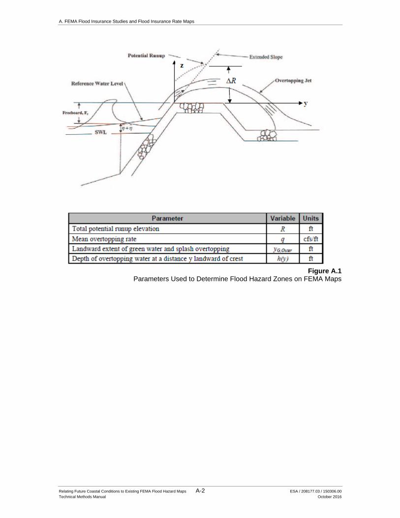
A. FEMA Flood Insurance Studies and Flood Insurance Rate Maps
Relating Future Coastal Conditions to Existing FEMA Flood Hazard Maps A-2 ESA / 208177.03 / 150306.00
Technical Methods Manual October 2016
Figure A.1
Parameters Used to Determine Flood Hazard Zones on FEMA Maps
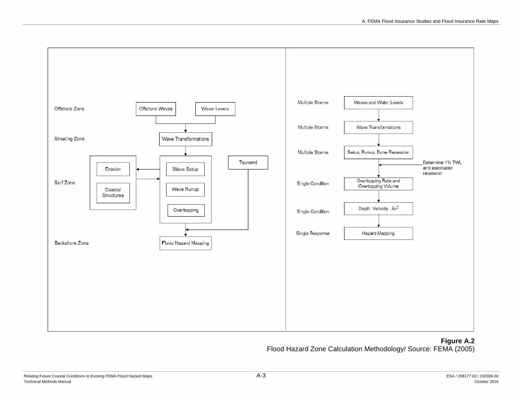
A. FEMA Flood Insurance Studies and Flood Insurance Rate Maps
Relating Future Coastal Conditions to Existing FEMA Flood Hazard Maps A-3 ESA / 208177.03 / 150306.00
Technical Methods Manual October 2016
Figure A.2 Flood Hazard Zone Calculation Methodology/ Source: FEMA (2005)
A. FEMA Flood Insurance Studies and Flood Insurance Rate Maps
Relating Future Coastal Conditions to Existing FEMA Flood Hazard Maps A-4 ESA / 208177.03 / 150306.00
Technical Methods Manual October 2016
The SIO projections (Appendix B) generally fit into this methodology up to and within the step
labeled “Wave Runup”. In particular, the SIO computations conform to the “response based
analysis” identified by the Guidelines (FEMA, 2005) for accurately computing the recurrence of
Pacific coast flood events38. The SIO methodology obviously differs from the present FEMA
approach by addressing future conditions. The SIO methodology uses one equation for flood
hazard, based on runup on a natural beach, where as FEMA requires application of a range of
methods depending on the shore geometry and dominate hazard (e.g. overtopping).
Figure A.3 is a schematic that shows how flood hazard zones are arranged, with the most
hazardous zone, called the V-Zone, being the most seaward where the waves first run up on the
shore. Typically the hazards decrease with distance landward, following the general route of
wave propagation and calculation sequence. Figure A.4 shows an example of the flood zones in
plan (map) view, and how the hazards computed for shore segments are merged to make a FIRM.
The SIO study “stops short” of providing the detailed consideration of local topography that
results in precise spatial resolution of flood hazards in FEMA maps. Other hazard projections,
such as future conditions of sea-level rise (Appendix C), provide useful information that also
diverge from FEMA mapping in terms of methodology, methods and resolution.
FEMA is evaluating methods to incorporate future sea levels in flood hazard mapping and has
recently completed a pilot study39. One of the sites considered in this pilot study, San Francisco,
is also an SIO output site as well as a site where other sea level rise hazard studies have produced
output.
Coastal hazards can become worse over time, newer maps are likely to be more representative of
existing conditions, and newer maps are often more precise. Older maps may not be useful in
establishing future conditions. Therefore, the user should start with the most up-to-date map,
consider when the map was made, and assess whether the map adequately represents existing
conditions. Figure A.5 shows older flood maps for California, circa 1982 and 1986. The 1982
map provides only approximate locations but based on the scale it is estimated that the V Zone
boundary varies by location and is about 200 to 400 feet seaward of Seadrift Road. No flood
elevations are given. The 1986 map indicates the V Zone is 100 to 200 feet from Seadrift Road
and the elevation is 19 to 20 feet (NAVD). Figure A.6 is the newest map and is provisional (not
yet effective, subject to revision). This new map indicates that the V Zone is at or very close to
Seadrift Road with an elevation of 19 to 22 feet (NAVD). These maps indicate that coastal
hazards can become worse over time, and that the newer maps are more precise. FEMA expects
to have new maps for the entire California coast within the next few years, and these maps are
expected to have resolutions adequate to apply the methods described in this manual, similar to
Figure A.6.
38 Garrity, Nicholas J., Robert Battalio PE, Peter J. Hawkes PhD, Dan Roupe, Evaluation Of Event And Response
Approaches To Estimate The 100-Year Coastal Flood For Pacific Coast Sheltered Waters, Proceedings of the 30th International Conference of Coastal Engineering, 2006, ASCE, 2007, Vol. 2, pp 1651-1663.
39 FEMA, 2105 in press, Sea Level Rise Pilot Study, Future Conditions Analysis and Mapping for San Francisco County, California, http://www.floods.org/Files/Conf2014_ppts/E7_Curtis.pdf.
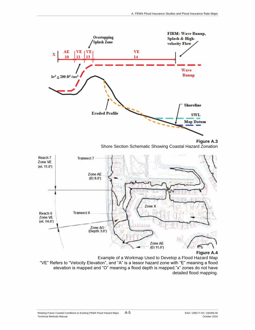
A. FEMA Flood Insurance Studies and Flood Insurance Rate Maps
Relating Future Coastal Conditions to Existing FEMA Flood Hazard Maps A-5 ESA / 208177.03 / 150306.00
Technical Methods Manual October 2016
Figure A.3
Shore Section Schematic Showing Coastal Hazard Zonation
Figure A.4
Example of a Workmap Used to Develop a Flood Hazard Map “VE” Refers to “Velocity Elevation”, and “A” is a lessor hazard zone with “E” meaning a flood
elevation is mapped and “O” meaning a flood depth is mapped.”x” zones do not have detailed flood mapping.
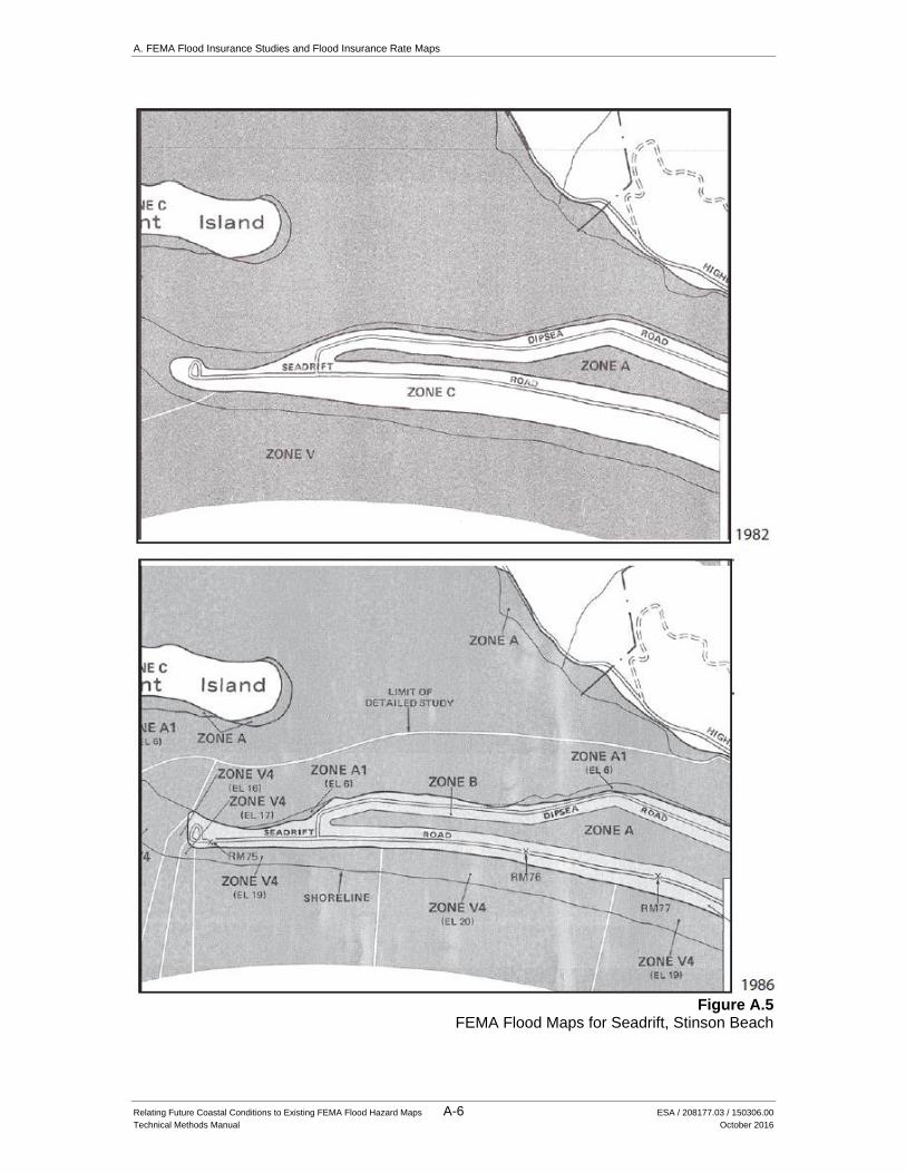
A. FEMA Flood Insurance Studies and Flood Insurance Rate Maps
Relating Future Coastal Conditions to Existing FEMA Flood Hazard Maps A-6 ESA / 208177.03 / 150306.00
Technical Methods Manual October 2016
Figure A.5
FEMA Flood Maps for Seadrift, Stinson Beach
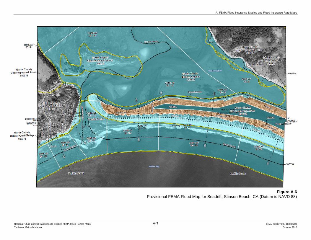
A. FEMA Flood Insurance Studies and Flood Insurance Rate Maps
Relating Future Coastal Conditions to Existing FEMA Flood Hazard Maps A-7 ESA / 208177.03 / 150306.00
Technical Methods Manual October 2016
Figure A.6
Provisional FEMA Flood Map for Seadrift, Stinson Beach, CA (Datum is NAVD 88)
A. FEMA Flood Insurance Studies and Flood Insurance Rate Maps
Relating Future Coastal Conditions to Existing FEMA Flood Hazard Maps A-8 ESA / 208177.03 / 150306.00
Technical Methods Manual October 2016
This page intentionally left blank
Relating Future Coastal Conditions to Existing FEMA Flood Hazard Maps B-1 ESA / 208177.03 / 150306.00
Technical Methods Manual October 2016
APPENDIX B
Scripps Institution of Oceanography (SIO) Future Waves and Water Levels
The purpose of Appendix B is to describe the future conditions modeling sufficiently for use in
estimating the increase in coastal flood hazards expected to result from climate change. This
Appendix also provides a comparison of SIO projections with historical conditions in order to
assess the extent to which components change in response to climate change, to quantify
differences that may affect comparisons to flood levels computed by FEMA, and to provide
sufficient detail to empower informed use consistent with professional practice.
Scientists from the Scripps Institution of Oceanography (SIO) provided future conditions based
on outputs from selected global circulation models (GCMs). These outputs consisted of future
waves and water levels for three offshore locations and associated wave runup and total water
levels for six nearshore locations along the California coast40. Secular sea level rise scenarios
were added based on recent guidance41.
1.0 SIO GCM-Based Future Waves and Water Levels
The SIO future conditions “outputs” consist of future ocean water levels (including non-tidal
constituents that affect flood levels) and wave-induced runup, and the summation of water level
and runup called Total Water Level (TWL). Methods are discussed in a prior report with the
following salient summary42:
“flooding is caused by short‐term processes superimposed on RSL (relative sea level
rise) and results from storm waves impacting the coast during the co‐occurrence of high
tides and storm surges, with El Niño–related interannual sea level increases augmenting
RSL. “
As discussed in Section 2 of this report, the SIO methodology is consistent with FEMA’s
methods for existing flood hazard mapping. SIO methods basically use forecasted data rather than
historical data to compute wave runup. Also, SIO methods have been applied for only a few
locations and have not been used to create hazard maps. The SIO projections are therefore, not
40 Bromirski, P. D., D. R. Cayan, N. Graham, R. E. Flick, and M. Tyree (Scripps Institution of Oceanography). 2012.
Coastal Flooding Potential Projections: 2000–2100. California Energy Commission. CEC‐ 500‐ 2012‐ 011. 41 NRC, 2012. 42 Bromirski, P. D., D. R. Cayan, N. Graham, R. E. Flick, and M. Tyree (Scripps Institution of Oceanography). 2012.
Coastal Flooding Potential Projections: 2000–2100. California Energy Commission. CEC‐ 500‐ 2012‐ 011.
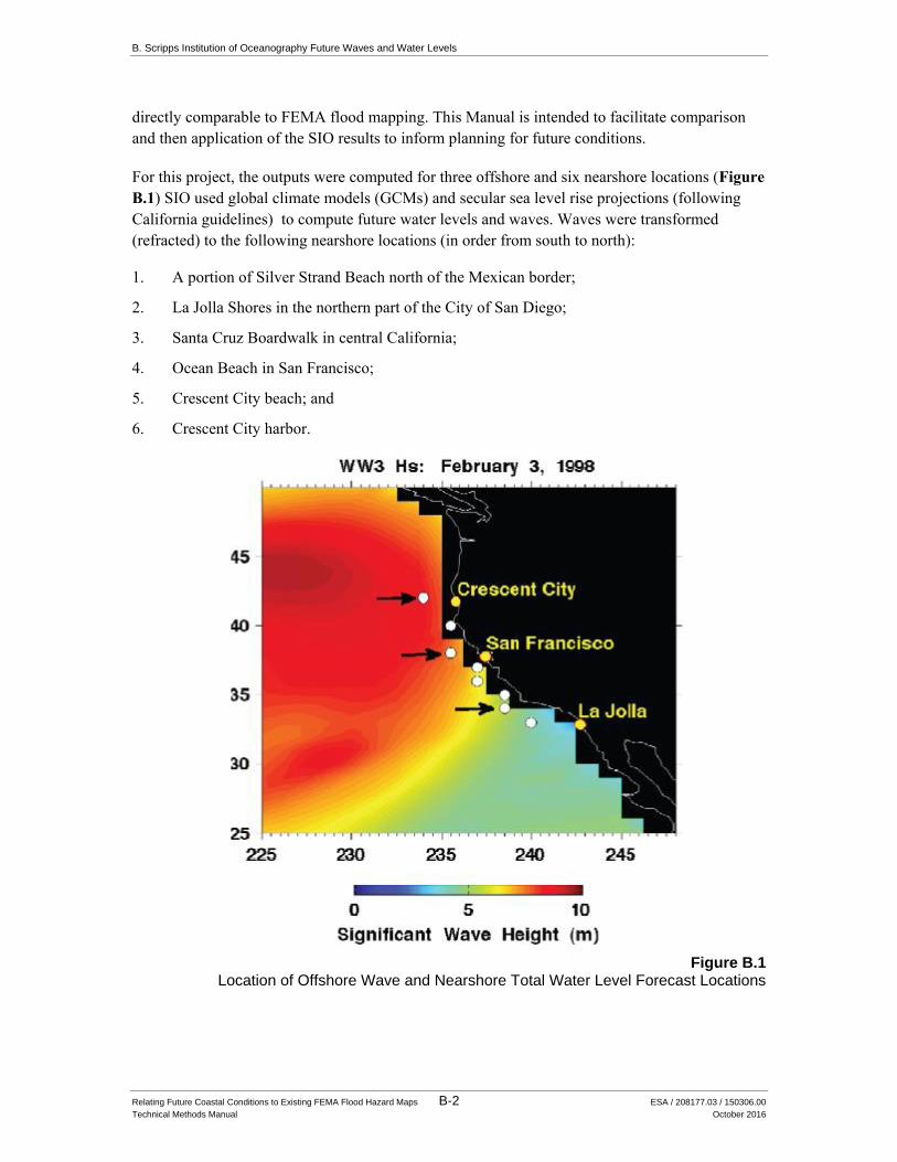
B. Scripps Institution of Oceanography Future Waves and Water Levels
Relating Future Coastal Conditions to Existing FEMA Flood Hazard Maps B-2 ESA / 208177.03 / 150306.00
Technical Methods Manual October 2016
directly comparable to FEMA flood mapping. This Manual is intended to facilitate comparison
and then application of the SIO results to inform planning for future conditions.
For this project, the outputs were computed for three offshore and six nearshore locations (Figure
B.1) SIO used global climate models (GCMs) and secular sea level rise projections (following
California guidelines) to compute future water levels and waves. Waves were transformed
(refracted) to the following nearshore locations (in order from south to north):
1. A portion of Silver Strand Beach north of the Mexican border;
2. La Jolla Shores in the northern part of the City of San Diego;
3. Santa Cruz Boardwalk in central California;
4. Ocean Beach in San Francisco;
5. Crescent City beach; and
6. Crescent City harbor.
Figure B.1
Location of Offshore Wave and Nearshore Total Water Level Forecast Locations
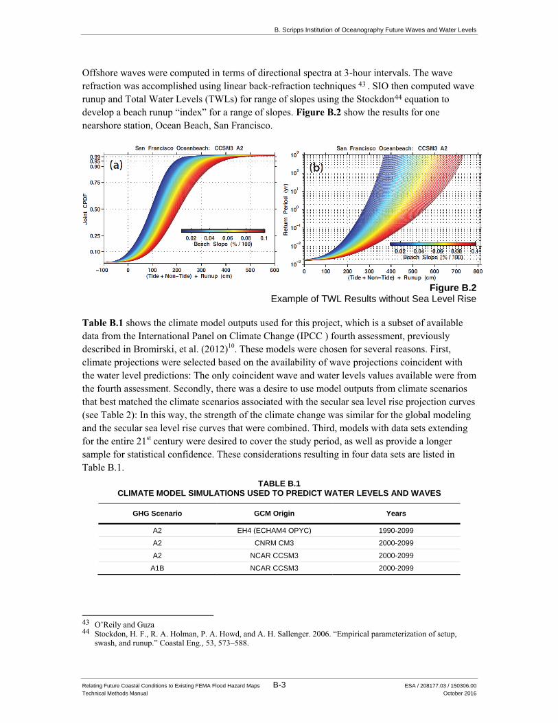
B. Scripps Institution of Oceanography Future Waves and Water Levels
Relating Future Coastal Conditions to Existing FEMA Flood Hazard Maps B-3 ESA / 208177.03 / 150306.00
Technical Methods Manual October 2016
Offshore waves were computed in terms of directional spectra at 3-hour intervals. The wave
refraction was accomplished using linear back-refraction techniques 43 . SIO then computed wave
runup and Total Water Levels (TWLs) for range of slopes using the Stockdon44 equation to
develop a beach runup “index” for a range of slopes. Figure B.2 show the results for one
nearshore station, Ocean Beach, San Francisco.
Figure B.2
Example of TWL Results without Sea Level Rise
Table B.1 shows the climate model outputs used for this project, which is a subset of available
data from the International Panel on Climate Change (IPCC ) fourth assessment, previously
described in Bromirski, et al. (2012)10. These models were chosen for several reasons. First,
climate projections were selected based on the availability of wave projections coincident with
the water level predictions: The only coincident wave and water levels values available were from
the fourth assessment. Secondly, there was a desire to use model outputs from climate scenarios
that best matched the climate scenarios associated with the secular sea level rise projection curves
(see Table 2): In this way, the strength of the climate change was similar for the global modeling
and the secular sea level rise curves that were combined. Third, models with data sets extending
for the entire 21st century were desired to cover the study period, as well as provide a longer
sample for statistical confidence. These considerations resulting in four data sets are listed in
Table B.1.
TABLE B.1 CLIMATE MODEL SIMULATIONS USED TO PREDICT WATER LEVELS AND WAVES
GHG Scenario GCM Origin Years
A2 EH4 (ECHAM4 OPYC) 1990-2099
A2 CNRM CM3 2000-2099
A2 NCAR CCSM3 2000-2099
A1B NCAR CCSM3 2000-2099
43 O’Reily and Guza 44 Stockdon, H. F., R. A. Holman, P. A. Howd, and A. H. Sallenger. 2006. “Empirical parameterization of setup,
swash, and runup.” Coastal Eng., 53, 573–588.
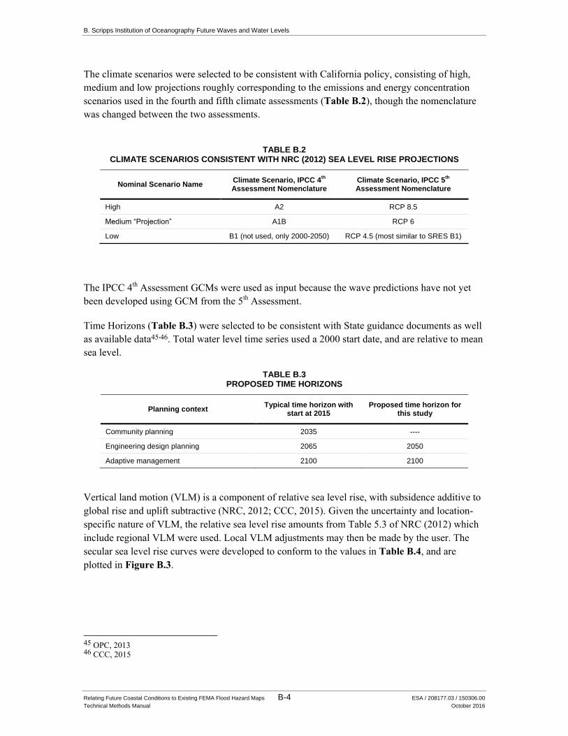
B. Scripps Institution of Oceanography Future Waves and Water Levels
Relating Future Coastal Conditions to Existing FEMA Flood Hazard Maps B-4 ESA / 208177.03 / 150306.00
Technical Methods Manual October 2016
The climate scenarios were selected to be consistent with California policy, consisting of high,
medium and low projections roughly corresponding to the emissions and energy concentration
scenarios used in the fourth and fifth climate assessments (Table B.2), though the nomenclature
was changed between the two assessments.
TABLE B.2 CLIMATE SCENARIOS CONSISTENT WITH NRC (2012) SEA LEVEL RISE PROJECTIONS
Nominal Scenario Name Climate Scenario, IPCC 4
th
Assessment Nomenclature Climate Scenario, IPCC 5
th
Assessment Nomenclature
High A2 RCP 8.5
Medium “Projection” A1B RCP 6
Low B1 (not used, only 2000-2050) RCP 4.5 (most similar to SRES B1)
The IPCC 4th Assessment GCMs were used as input because the wave predictions have not yet
been developed using GCM from the 5th Assessment.
Time Horizons (Table B.3) were selected to be consistent with State guidance documents as well
as available data45,46. Total water level time series used a 2000 start date, and are relative to mean
sea level.
TABLE B.3 PROPOSED TIME HORIZONS
Planning context Typical time horizon with
start at 2015 Proposed time horizon for
this study
Community planning 2035 ----
Engineering design planning 2065 2050
Adaptive management 2100 2100
Vertical land motion (VLM) is a component of relative sea level rise, with subsidence additive to
global rise and uplift subtractive (NRC, 2012; CCC, 2015). Given the uncertainty and location-
specific nature of VLM, the relative sea level rise amounts from Table 5.3 of NRC (2012) which
include regional VLM were used. Local VLM adjustments may then be made by the user. The
secular sea level rise curves were developed to conform to the values in Table B.4, and are
plotted in Figure B.3.
45 OPC, 2013 46 CCC, 2015
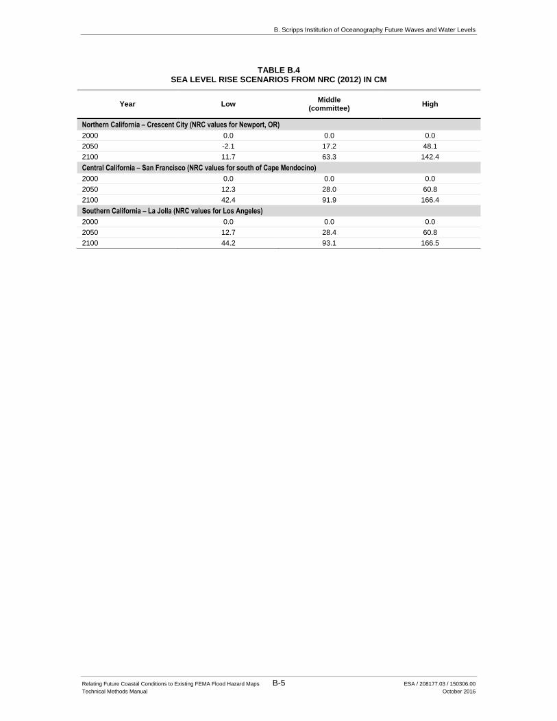
B. Scripps Institution of Oceanography Future Waves and Water Levels
Relating Future Coastal Conditions to Existing FEMA Flood Hazard Maps B-5 ESA / 208177.03 / 150306.00
Technical Methods Manual October 2016
TABLE B.4 SEA LEVEL RISE SCENARIOS FROM NRC (2012) IN CM
Year Low Middle
(committee) High
Northern California – Crescent City (NRC values for Newport, OR)
2000 0.0 0.0 0.0
2050 -2.1 17.2 48.1
2100 11.7 63.3 142.4
Central California – San Francisco (NRC values for south of Cape Mendocino)
2000 0.0 0.0 0.0
2050 12.3 28.0 60.8
2100 42.4 91.9 166.4
Southern California – La Jolla (NRC values for Los Angeles)
2000 0.0 0.0 0.0
2050 12.7 28.4 60.8
2100 44.2 93.1 166.5
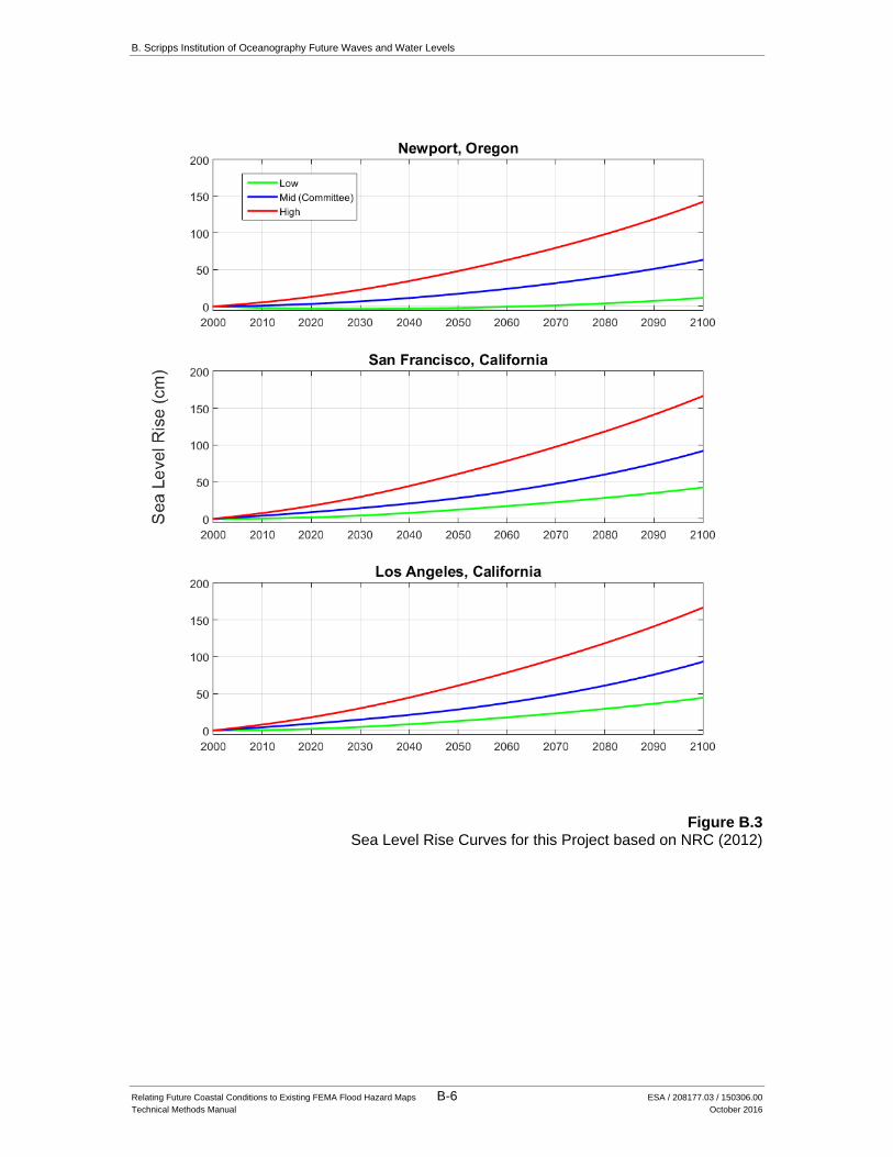
B. Scripps Institution of Oceanography Future Waves and Water Levels
Relating Future Coastal Conditions to Existing FEMA Flood Hazard Maps B-6 ESA / 208177.03 / 150306.00
Technical Methods Manual October 2016
Figure B.3
Sea Level Rise Curves for this Project based on NRC (2012)
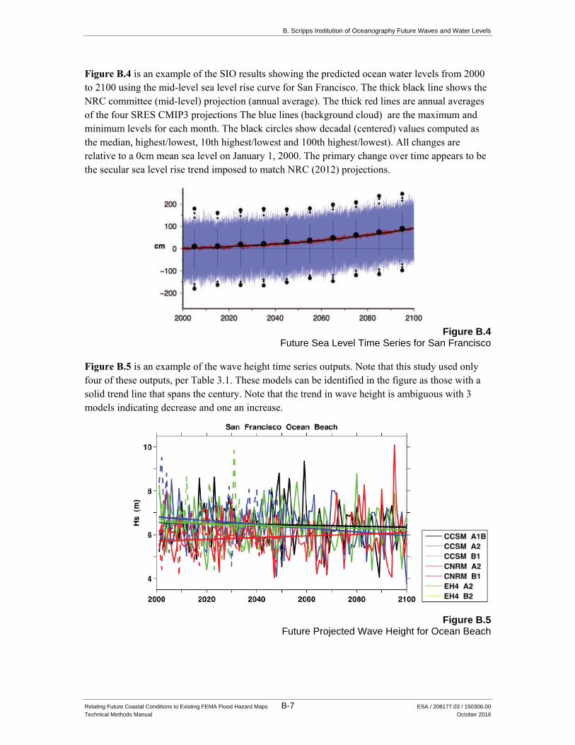
B. Scripps Institution of Oceanography Future Waves and Water Levels
Relating Future Coastal Conditions to Existing FEMA Flood Hazard Maps B-7 ESA / 208177.03 / 150306.00
Technical Methods Manual October 2016
Figure B.4 is an example of the SIO results showing the predicted ocean water levels from 2000
to 2100 using the mid-level sea level rise curve for San Francisco. The thick black line shows the
NRC committee (mid-level) projection (annual average). The thick red lines are annual averages
of the four SRES CMIP3 projections The blue lines (background cloud) are the maximum and
minimum levels for each month. The black circles show decadal (centered) values computed as
the median, highest/lowest, 10th highest/lowest and 100th highest/lowest). All changes are
relative to a 0cm mean sea level on January 1, 2000. The primary change over time appears to be
the secular sea level rise trend imposed to match NRC (2012) projections.
Figure B.4
Future Sea Level Time Series for San Francisco
Figure B.5 is an example of the wave height time series outputs. Note that this study used only
four of these outputs, per Table 3.1. These models can be identified in the figure as those with a
solid trend line that spans the century. Note that the trend in wave height is ambiguous with 3
models indicating decrease and one an increase.
Figure B.5 Future Projected Wave Height for Ocean Beach
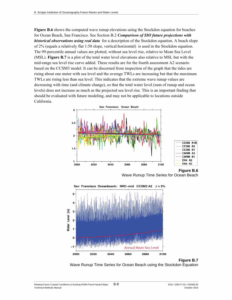
B. Scripps Institution of Oceanography Future Waves and Water Levels
Relating Future Coastal Conditions to Existing FEMA Flood Hazard Maps B-8 ESA / 208177.03 / 150306.00
Technical Methods Manual October 2016
Figure B.6 shows the computed wave runup elevations using the Stockdon equation for beaches
for Ocean Beach, San Francisco. See Section B.2 Comparison of SIO future projections with
historical observations using real data for a description of the Stockdon equation. A beach slope
of 2% (equals a relatively flat 1:50 slope, vertical:horizontal) is used in the Stockdon equation.
The 99-percentile annual values are plotted, without sea level rise, relative to Mean Sea Level
(MSL). Figure B.7 is a plot of the total water level elevations also relative to MSL but with the
mid-range sea level rise curve added. These results are for the fourth assessment A2 scenario
based on the CCSM3 model. It can be discerned from inspection of the graph that the tides are
rising about one meter with sea level and the average TWLs are increasing but that the maximum
TWLs are rising less than sea level. This indicates that the extreme wave runup values are
decreasing with time (and climate change), so that the total water level (sum of runup and ocean
levels) does not increase as much as the projected sea level rise. This is an important finding that
should be evaluated with future modeling, and may not be applicable to locations outside
California.
Figure B.6 Wave Runup Time Series for Ocean Beach
Figure B.7 Wave Runup Time Series for Ocean Beach using the Stockdon Equation
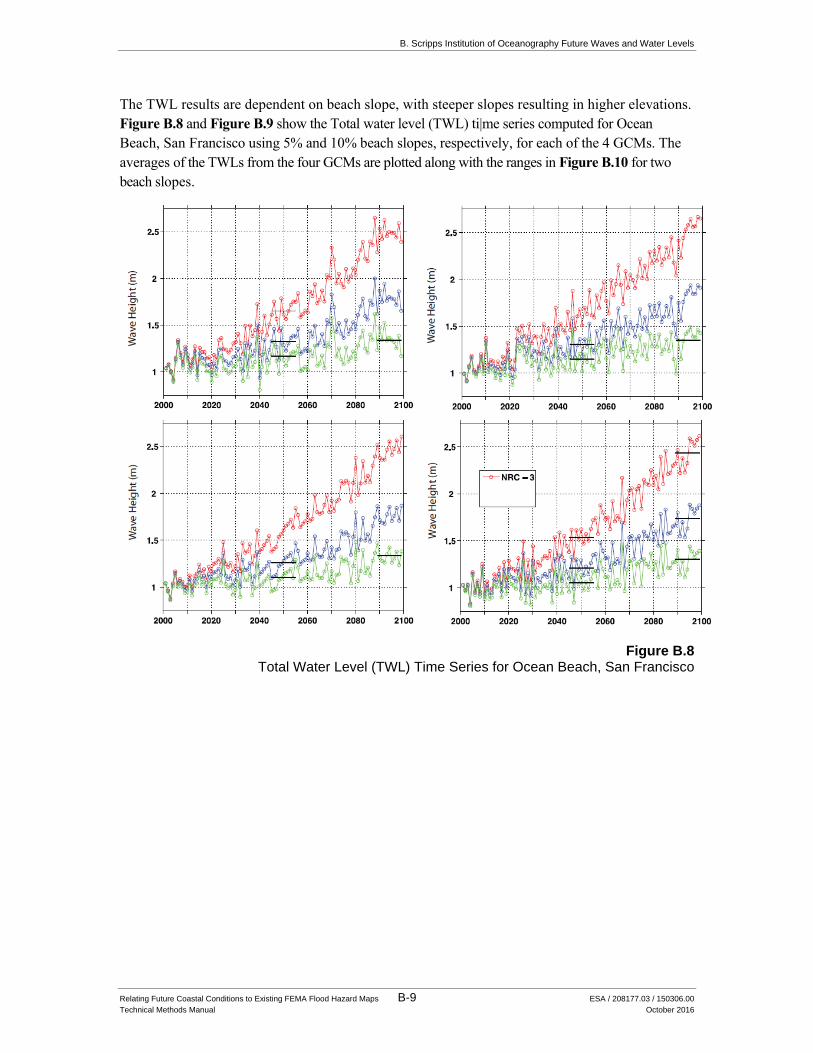
B. Scripps Institution of Oceanography Future Waves and Water Levels
Relating Future Coastal Conditions to Existing FEMA Flood Hazard Maps B-9 ESA / 208177.03 / 150306.00
Technical Methods Manual October 2016
The TWL results are dependent on beach slope, with steeper slopes resulting in higher elevations.
Figure B.8 and Figure B.9 show the Total water level (TWL) ti|me series computed for Ocean
Beach, San Francisco using 5% and 10% beach slopes, respectively, for each of the 4 GCMs. The
averages of the TWLs from the four GCMs are plotted along with the ranges in Figure B.10 for two
beach slopes.
Figure B.8 Total Water Level (TWL) Time Series for Ocean Beach, San Francisco

B. Scripps Institution of Oceanography Future Waves and Water Levels
Relating Future Coastal Conditions to Existing FEMA Flood Hazard Maps B-10 ESA / 208177.03 / 150306.00
Technical Methods Manual October 2016
Figure B.9 Wave height time series for Ocean Beach, San Francisco for different GCMs
Figure B.10
Total Water Level (TWL) Time Series for Ocean Beach, San Francisco Computed with Beach Slopes of 2% (Left) and 5% (Right)
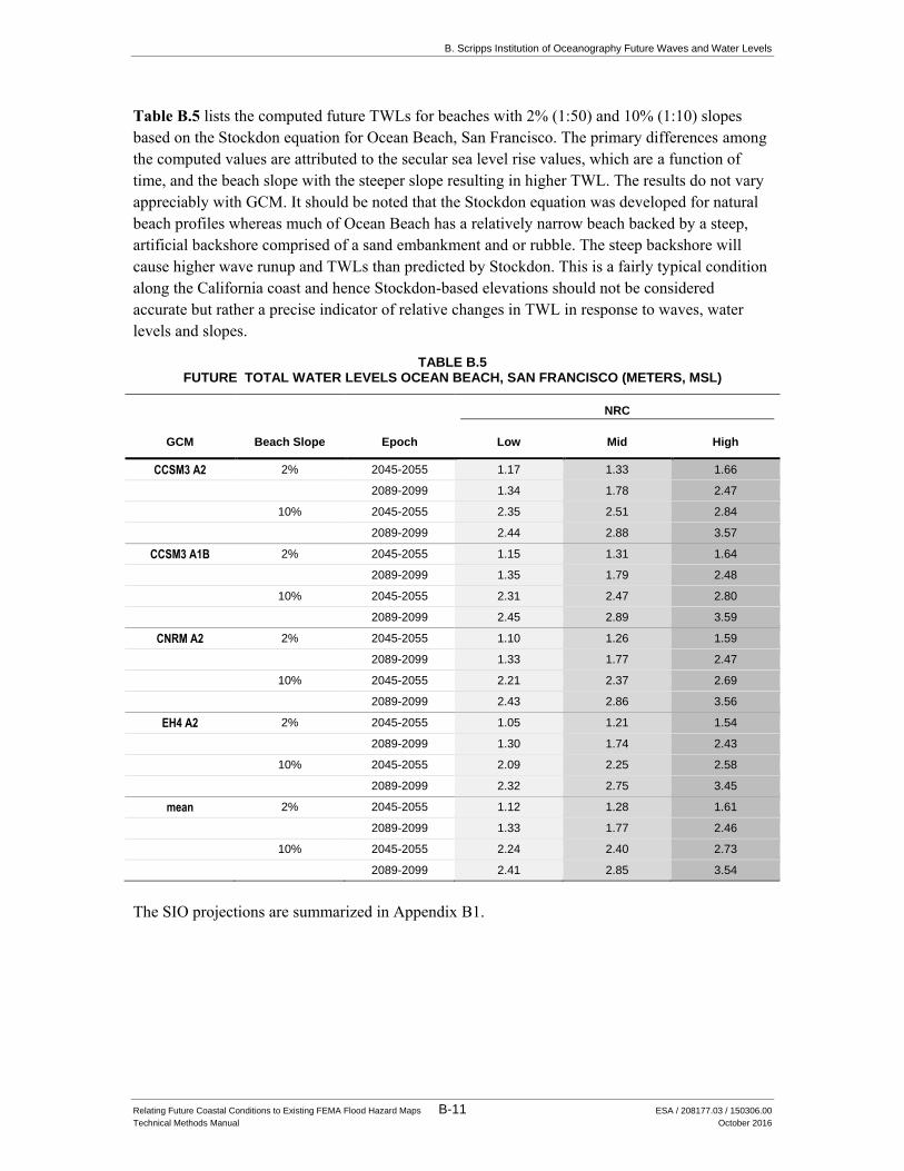
B. Scripps Institution of Oceanography Future Waves and Water Levels
Relating Future Coastal Conditions to Existing FEMA Flood Hazard Maps B-11 ESA / 208177.03 / 150306.00
Technical Methods Manual October 2016
Table B.5 lists the computed future TWLs for beaches with 2% (1:50) and 10% (1:10) slopes
based on the Stockdon equation for Ocean Beach, San Francisco. The primary differences among
the computed values are attributed to the secular sea level rise values, which are a function of
time, and the beach slope with the steeper slope resulting in higher TWL. The results do not vary
appreciably with GCM. It should be noted that the Stockdon equation was developed for natural
beach profiles whereas much of Ocean Beach has a relatively narrow beach backed by a steep,
artificial backshore comprised of a sand embankment and or rubble. The steep backshore will
cause higher wave runup and TWLs than predicted by Stockdon. This is a fairly typical condition
along the California coast and hence Stockdon-based elevations should not be considered
accurate but rather a precise indicator of relative changes in TWL in response to waves, water
levels and slopes.
TABLE B.5 FUTURE TOTAL WATER LEVELS OCEAN BEACH, SAN FRANCISCO (METERS, MSL)
NRC
GCM Beach Slope Epoch Low Mid High
CCSM3 A2 2% 2045-2055 1.17 1.33 1.66
2089-2099 1.34 1.78 2.47
10% 2045-2055 2.35 2.51 2.84
2089-2099 2.44 2.88 3.57
CCSM3 A1B 2% 2045-2055 1.15 1.31 1.64
2089-2099 1.35 1.79 2.48
10% 2045-2055 2.31 2.47 2.80
2089-2099 2.45 2.89 3.59
CNRM A2 2% 2045-2055 1.10 1.26 1.59
2089-2099 1.33 1.77 2.47
10% 2045-2055 2.21 2.37 2.69
2089-2099 2.43 2.86 3.56
EH4 A2 2% 2045-2055 1.05 1.21 1.54
2089-2099 1.30 1.74 2.43
10% 2045-2055 2.09 2.25 2.58
2089-2099 2.32 2.75 3.45
mean 2% 2045-2055 1.12 1.28 1.61
2089-2099 1.33 1.77 2.46
10% 2045-2055 2.24 2.40 2.73
2089-2099 2.41 2.85 3.54
The SIO projections are summarized in Appendix B1.
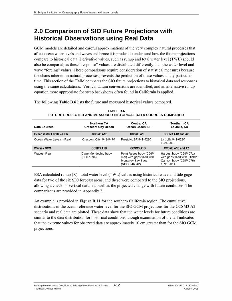
B. Scripps Institution of Oceanography Future Waves and Water Levels
Relating Future Coastal Conditions to Existing FEMA Flood Hazard Maps B-12 ESA / 208177.03 / 150306.00
Technical Methods Manual October 2016
2.0 Comparison of SIO Future Projections with Historical Observations using Real Data
GCM models are detailed and careful approximations of the very complex natural processes that
affect ocean water levels and waves and hence it is prudent to understand how the future projections
compare to historical data. Derivative values, such as runup and total water level (TWL) should
also be compared, as these “response” values are distributed differently than the water level and
wave “forcing” values. These comparisons require consideration of statistical measures because
the chaos inherent in natural processes prevents the prediction of these values at any particular
time. This section of the TMM compares the SIO future projections to historical data and responses
using the same calculations. Vertical datum conversions are identified, and an alternative runup
equation more appropriate for steep backshores often found in California is applied.
The following Table B.6 lists the future and measured historical values compared.
TABLE B.6 FUTURE PROJECTED AND MEASURED HISTORICAL DATA SOURCES COMPARED
Data Sources Northern CA
Crescent City Beach Central CA
Ocean Beach, SF Southern CA La Jolla, SD
Ocean Water Levels – GCM CCSM3 A1B CCSM3 A1B CCSM3 A1B and A2
Ocean Water Levels - Real Crescent City, 941-9470 Presidio, SF 941-4290 La Jolla 941-0230 1924-2015
Waves - GCM CCSM3 A1B CCSM3 A1B CCSM3 A1B and A2
Waves- Real Cape Mendocino buoy (CDIP 094)
Point Reyes buoy (CDIP 029) with gaps filled with Monterey Bay Buoy (NDBC 46042)
Harvest buoy (CDIP 071) with gaps filled with Diablo Canyon buoy (CDIP 076) 1991-2014
ESA calculated runup (R) total water level (TWL) values using historical wave and tide gage
data for two of the six SIO forecast areas, and these were compared to the SIO projections,
allowing a check on vertical datum as well as the projected change with future conditions. The
comparisons are provided in Appendix 2.
An example is provided in Figure B.11 for the southern California region. The cumulative
distributions of the ocean reference water level for the SIO GCM projections for the CCSM3 A2
scenario and real data are plotted. These data show that the water levels for future conditions are
similar to the data distribution for historical conditions, though examination of the tail indicates
that the extreme values for observed data are approximately 10 cm greater than for the SIO GCM
projections.
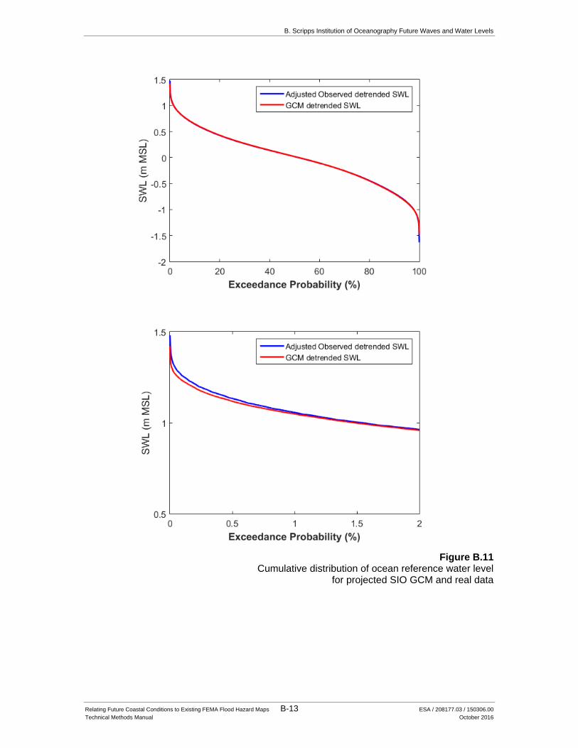
B. Scripps Institution of Oceanography Future Waves and Water Levels
Relating Future Coastal Conditions to Existing FEMA Flood Hazard Maps B-13 ESA / 208177.03 / 150306.00
Technical Methods Manual October 2016
Figure B.11
Cumulative distribution of ocean reference water level for projected SIO GCM and real data
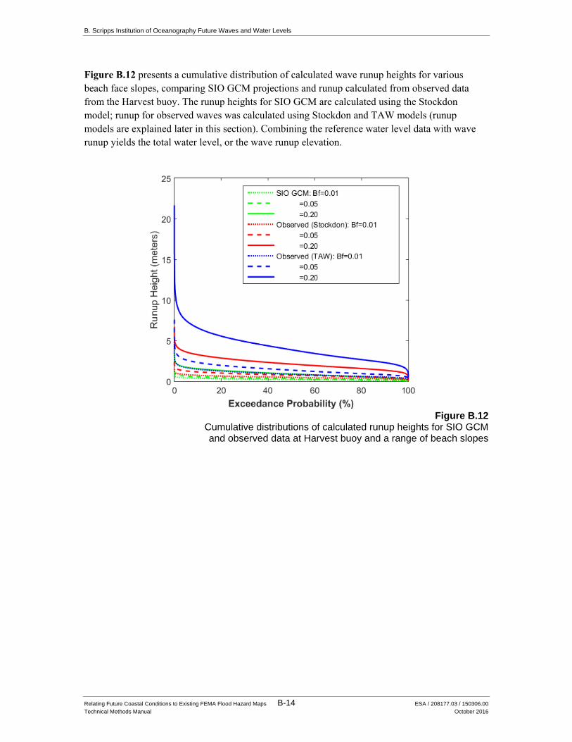
B. Scripps Institution of Oceanography Future Waves and Water Levels
Relating Future Coastal Conditions to Existing FEMA Flood Hazard Maps B-14 ESA / 208177.03 / 150306.00
Technical Methods Manual October 2016
Figure B.12 presents a cumulative distribution of calculated wave runup heights for various
beach face slopes, comparing SIO GCM projections and runup calculated from observed data
from the Harvest buoy. The runup heights for SIO GCM are calculated using the Stockdon
model; runup for observed waves was calculated using Stockdon and TAW models (runup
models are explained later in this section). Combining the reference water level data with wave
runup yields the total water level, or the wave runup elevation.
Figure B.12
Cumulative distributions of calculated runup heights for SIO GCM and observed data at Harvest buoy and a range of beach slopes
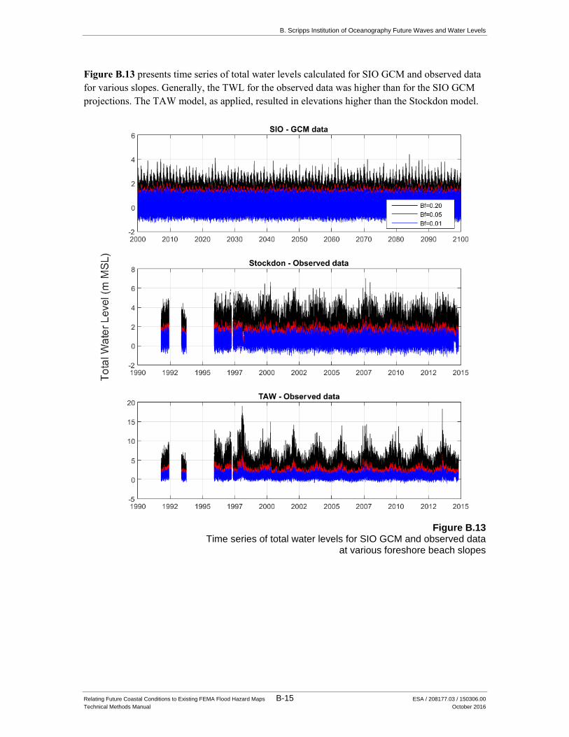
B. Scripps Institution of Oceanography Future Waves and Water Levels
Relating Future Coastal Conditions to Existing FEMA Flood Hazard Maps B-15 ESA / 208177.03 / 150306.00
Technical Methods Manual October 2016
Figure B.13 presents time series of total water levels calculated for SIO GCM and observed data
for various slopes. Generally, the TWL for the observed data was higher than for the SIO GCM
projections. The TAW model, as applied, resulted in elevations higher than the Stockdon model.
Figure B.13
Time series of total water levels for SIO GCM and observed data at various foreshore beach slopes
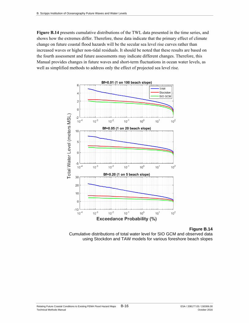
B. Scripps Institution of Oceanography Future Waves and Water Levels
Relating Future Coastal Conditions to Existing FEMA Flood Hazard Maps B-16 ESA / 208177.03 / 150306.00
Technical Methods Manual October 2016
Figure B.14 presents cumulative distributions of the TWL data presented in the time series, and
shows how the extremes differ. Therefore, these data indicate that the primary effect of climate
change on future coastal flood hazards will be the secular sea level rise curves rather than
increased waves or higher non-tidal residuals. It should be noted that these results are based on
the fourth assessment and future assessments may indicate different changes. Therefore, this
Manual provides changes in future waves and short-term fluctuations in ocean water levels, as
well as simplified methods to address only the effect of projected sea level rise.
Figure B.14
Cumulative distributions of total water level for SIO GCM and observed data using Stockdon and TAW models for various foreshore beach slopes
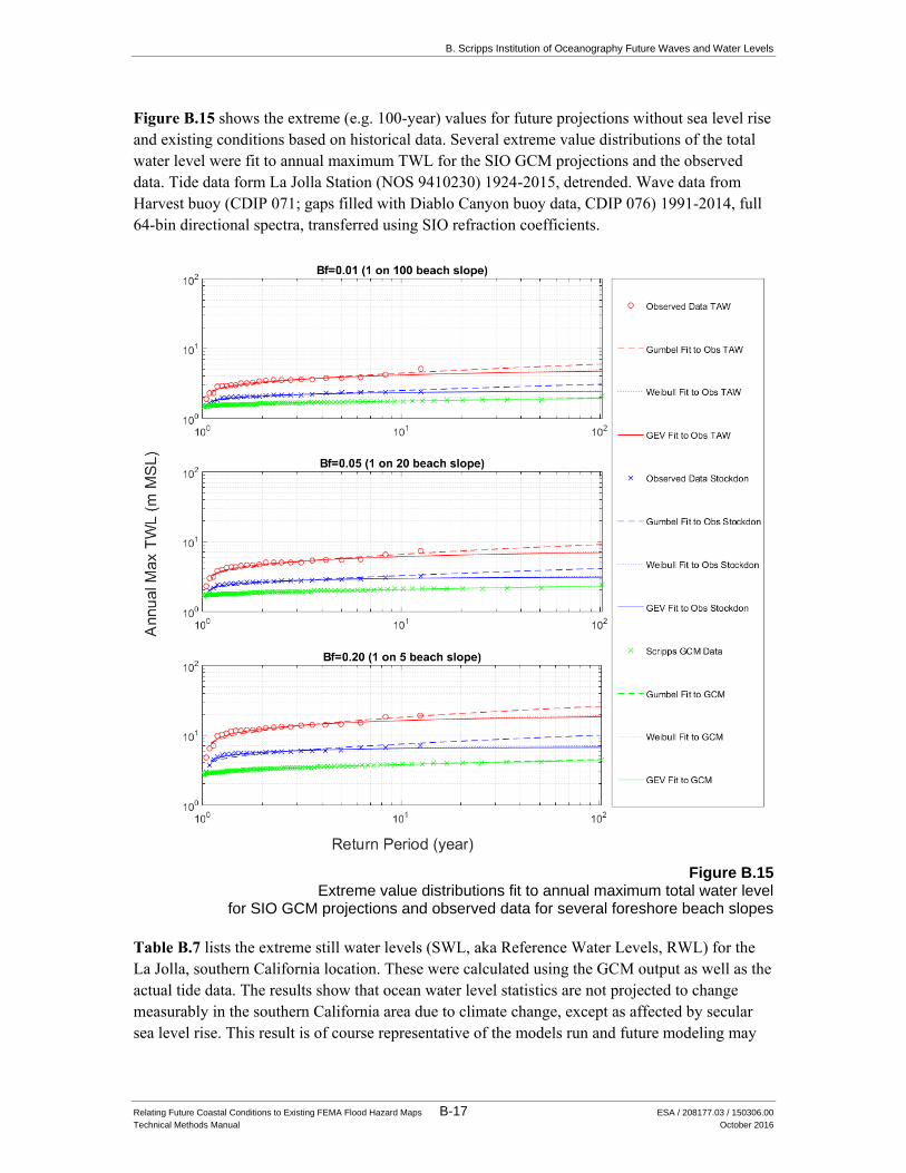
B. Scripps Institution of Oceanography Future Waves and Water Levels
Relating Future Coastal Conditions to Existing FEMA Flood Hazard Maps B-17 ESA / 208177.03 / 150306.00
Technical Methods Manual October 2016
Figure B.15 shows the extreme (e.g. 100-year) values for future projections without sea level rise
and existing conditions based on historical data. Several extreme value distributions of the total
water level were fit to annual maximum TWL for the SIO GCM projections and the observed
data. Tide data form La Jolla Station (NOS 9410230) 1924-2015, detrended. Wave data from
Harvest buoy (CDIP 071; gaps filled with Diablo Canyon buoy data, CDIP 076) 1991-2014, full
64-bin directional spectra, transferred using SIO refraction coefficients.
Figure B.15
Extreme value distributions fit to annual maximum total water level for SIO GCM projections and observed data for several foreshore beach slopes
Table B.7 lists the extreme still water levels (SWL, aka Reference Water Levels, RWL) for the
La Jolla, southern California location. These were calculated using the GCM output as well as the
actual tide data. The results show that ocean water level statistics are not projected to change
measurably in the southern California area due to climate change, except as affected by secular
sea level rise. This result is of course representative of the models run and future modeling may
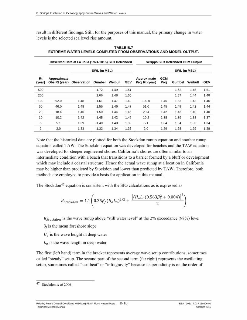
B. Scripps Institution of Oceanography Future Waves and Water Levels
Relating Future Coastal Conditions to Existing FEMA Flood Hazard Maps B-18 ESA / 208177.03 / 150306.00
Technical Methods Manual October 2016
result in different findings. Still, for the purposes of this manual, the primary change in water
levels is the selected sea level rise amount.
TABLE B.7 EXTREME WATER LEVELS COMPUTED FROM OBSERVATIONS AND MODEL OUTPUT.
Observed Data at La Jolla (1924-2015) SLR Detrended Scripps SLR Detrended GCM Output
Rt (year)
Approximate Obs Rt (year)
SWL (m MSL)
Approximate Proj Rt (year)
SWL (m MSL)
Observation Gumbel Weibull GEV GCM Proj Gumbel Weibull GEV
500 1.72 1.49 1.51 1.62 1.45 1.51
200 1.66 1.48 1.50 1.57 1.44 1.48
100 92.0 1.48 1.61 1.47 1.49 102.0 1.46 1.53 1.43 1.46
50 46.0 1.48 1.56 1.46 1.47 51.0 1.45 1.49 1.42 1.44
20 18.4 1.46 1.50 1.44 1.45 20.4 1.42 1.43 1.40 1.40
10 10.2 1.42 1.45 1.42 1.42 10.2 1.38 1.39 1.38 1.37
5 5.1 1.39 1.40 1.40 1.39 5.1 1.34 1.34 1.35 1.34
2 2.0 1.33 1.32 1.34 1.33 2.0 1.29 1.28 1.29 1.28
Note that the historical data are plotted for both the Stockdon runup equation and another runup
equation called TAW. The Stockdon equation was developed for beaches and the TAW equation
was developed for steeper engineered shores. California’s shores are often similar to an
intermediate condition with a beach that transitions to a barrier formed by a bluff or development
which may include a coastal structure. Hence the actual wave runup at a location in California
may be higher than predicted by Stockdon and lower than predicted by TAW. Therefore, both
methods are employed to provide a basis for application in this manual.
The Stockdon47 equation is consistent with the SIO calculations as is expressed as
𝑅𝑆𝑡𝑜𝑐𝑘𝑑𝑜𝑛 = 1.1 (0.35𝛽𝑓(𝐻𝑜𝐿𝑜)1/2 + [(𝐻𝑜𝐿𝑜(0.563𝛽𝑓
2 + 0.004)]2
2)
𝑅𝑆𝑡𝑜𝑐𝑘𝑑𝑜𝑛 is the wave runup above “still water level” at the 2% exceedance (98%) level
βf is the mean foreshore slope
𝐻𝑜 is the wave height in deep water
𝐿𝑜 is the wave length in deep water
The first (left hand) term in the bracket represents average wave setup contributions, sometimes
called “steady” setup. The second part of the second term (far right) represents the oscillating
setup, sometimes called “surf beat” or “infragravity” because its periodicity is on the order of
47 Stockdon et al 2006
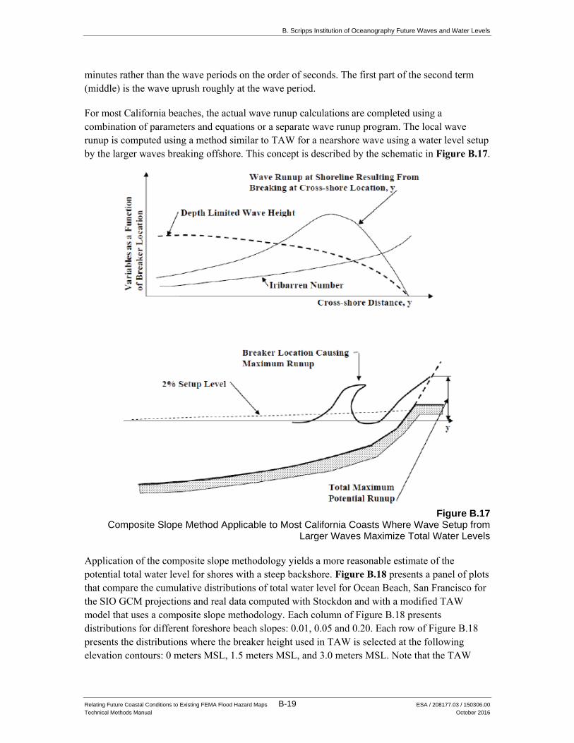
B. Scripps Institution of Oceanography Future Waves and Water Levels
Relating Future Coastal Conditions to Existing FEMA Flood Hazard Maps B-19 ESA / 208177.03 / 150306.00
Technical Methods Manual October 2016
minutes rather than the wave periods on the order of seconds. The first part of the second term
(middle) is the wave uprush roughly at the wave period.
For most California beaches, the actual wave runup calculations are completed using a
combination of parameters and equations or a separate wave runup program. The local wave
runup is computed using a method similar to TAW for a nearshore wave using a water level setup
by the larger waves breaking offshore. This concept is described by the schematic in Figure B.17.
Figure B.17
Composite Slope Method Applicable to Most California Coasts Where Wave Setup from Larger Waves Maximize Total Water Levels
Application of the composite slope methodology yields a more reasonable estimate of the
potential total water level for shores with a steep backshore. Figure B.18 presents a panel of plots
that compare the cumulative distributions of total water level for Ocean Beach, San Francisco for
the SIO GCM projections and real data computed with Stockdon and with a modified TAW
model that uses a composite slope methodology. Each column of Figure B.18 presents
distributions for different foreshore beach slopes: 0.01, 0.05 and 0.20. Each row of Figure B.18
presents the distributions where the breaker height used in TAW is selected at the following
elevation contours: 0 meters MSL, 1.5 meters MSL, and 3.0 meters MSL. Note that the TAW
B. Scripps Institution of Oceanography Future Waves and Water Levels
Relating Future Coastal Conditions to Existing FEMA Flood Hazard Maps B-20 ESA / 208177.03 / 150306.00
Technical Methods Manual October 2016
runup values decrease with an increase in the selected elevation contour for breaking. The total
water levels estimated with the modified TAW approach include a component that accounts for
the wave setup (using the parameterized DIM equation) and a swash component estimated using
the TAW equation48. The calculation of the dynamic water level, or wave setup, does not use the
foreshore slope, and is rather based on the overall slope of the shore profile. In this case, the
overall shore slopes used in the calculation of the 2% dynamic water level were 0.01, 0.02, and
0.05, corresponding to the foreshore beach slopes of 0.01, 0.05, and 0.20, respectively. A breaker
height was calculated based on the depth of the 2% dynamic water level at the selected breaker
elevation contour, and then applied to the runup calculation using the TAW method with a
backshore slope of 0.25 (a typical condition found along the California coast). Note also that the
Stockdon model predicts very large runup heights for the steep beach slope of 0.20, likely
because application of the empirical equation to this condition is out of the range of values for
which the equation was developed. The Stockdon equation is generally applicable for conditions
where R/H is less than 3, which has been shown by others to relate to conditions dominated by
infragravity processes where ξ<1.849 . This is shown by the graph of relative runup height as a
function of ξ in Figure B.16, for which the relative runup R/H is limited when the Iribarren
number is greater than 1.8 (this is a condition that occurs on a relatively steep slope with long
period waves): As the profile steepens and incidence processes start to dominate, the predicted
runup is defined by the flatter-sloped line to the right of the break in slope shown in the graph of
Figure B.16.
48 FEMA, 2005. Final Draft Guidelines for Coastal Flood Hazard Analysis and Mapping for the Pacific Coast of the
United States http://www.fema.gov/media-library-data/1389126436477-5bd6d5959718cf3f5a4b6e919f0c3b42/Guidelines%20for%20Coastal%20Flood%20Hazard%20Analysis%20and%20Mapping%20for%20the%20Pacific%20Coast%20of%20the%20United%20States%20%28Jan%202005%29.pdf
49 Laudier et al. Measured and modeled wave overtopping on a natural beach/ Coastal Engineering 58 (2011) 815–825
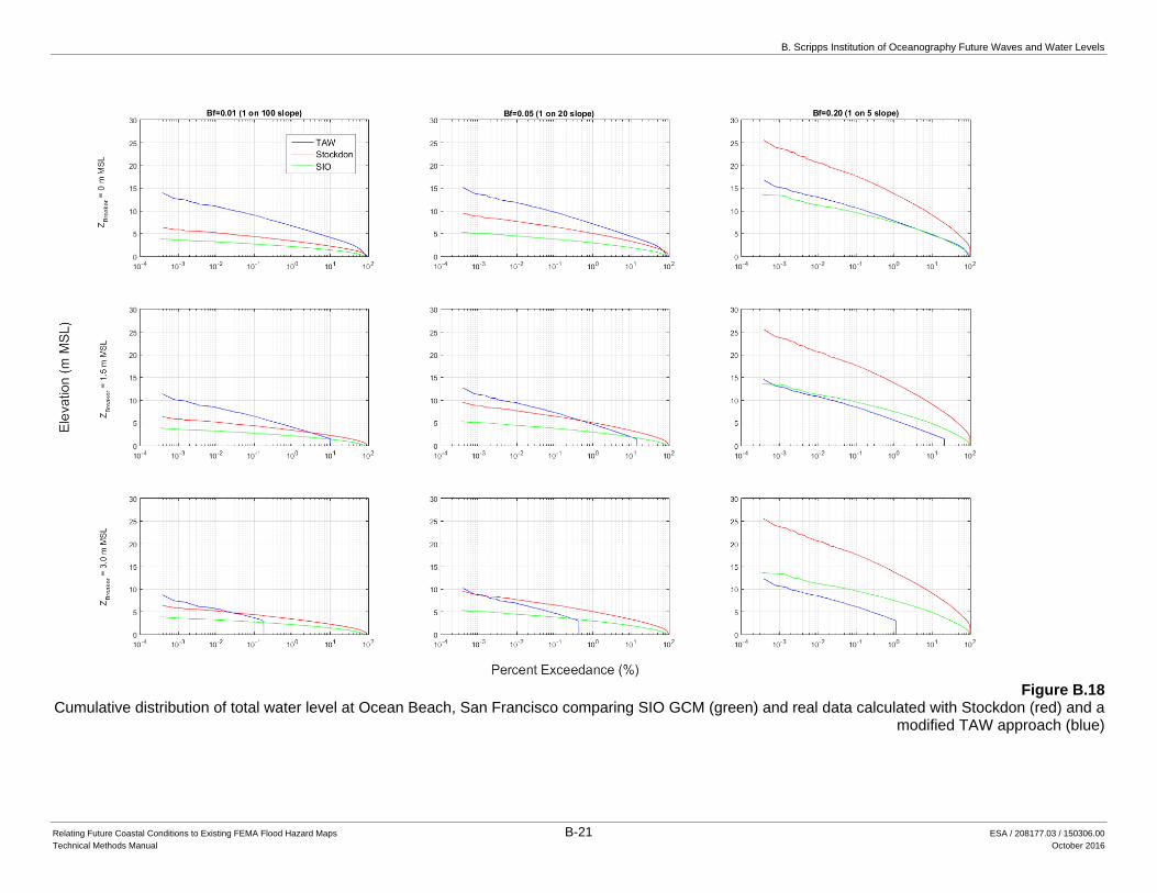
B. Scripps Institution of Oceanography Future Waves and Water Levels
Relating Future Coastal Conditions to Existing FEMA Flood Hazard Maps B-21 ESA / 208177.03 / 150306.00
Technical Methods Manual October 2016
Figure B.18
Cumulative distribution of total water level at Ocean Beach, San Francisco comparing SIO GCM (green) and real data calculated with Stockdon (red) and a modified TAW approach (blue)
B. Scripps Institution of Oceanography Future Waves and Water Levels
Relating Future Coastal Conditions to Existing FEMA Flood Hazard Maps B-22 ESA / 208177.03 / 150306.00
Technical Methods Manual October 2016
This page intentionally left blank
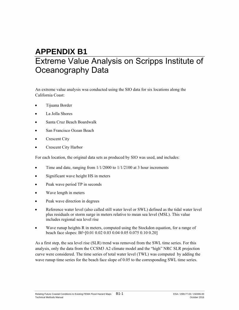
Relating Future Coastal Conditions to Existing FEMA Flood Hazard Maps B1-1 ESA / 208177.03 / 150306.00
Technical Methods Manual October 2016
APPENDIX B1
Extreme Value Analysis on Scripps Institute of Oceanography Data
An extreme value analysis wsa conducted using the SIO data for six locations along the
California Coast:
Tijuana Border
La Jolla Shores
Santa Cruz Beach Boardwalk
San Francisco Ocean Beach
Crescent City
Crescent City Harbor
For each location, the original data sets as produced by SIO was used, and includes:
Time and date, ranging from 1/1/2000 to 1/1/2100 at 3 hour increments
Significant wave height HS in meters
Peak wave period TP in seconds
Wave length in meters
Peak wave direction in degrees
Reference water level (also called still water level or SWL) defined as the tidal water level
plus residuals or storm surge in meters relative to mean sea level (MSL). This value
includes regional sea level rise
Wave runup heights R in meters, computed using the Stockdon equation, for a range of
beach face slopes: Bf=[0.01 0.02 0.03 0.04 0.05 0.075 0.10 0.20]
As a first step, the sea level rise (SLR) trend was removed from the SWL time series. For this
analysis, only the data from the CCSM3 A2 climate model and the “high” NRC SLR projection
curve were considered. The time series of total water level (TWL) was computed by adding the
wave runup time series for the beach face slope of 0.05 to the corresponding SWL time series.
B1. Extreme Value Analysis on SIO Oceanography Data
Relating Future Coastal Conditions to Existing FEMA Flood Hazard Maps B1-2 ESA / 208177.03 / 150306.00
Technical Methods Manual October 2016
The extreme value analysis considered annual maximum events based on a water year, a period
from October 1 through September 30. Plots of the extreme values for the SWL were developed
for wave runup height R (for Bf=0.05) and TWL. These plots are presented below for all six
locations.
Results of the extreme values are tabulated for each of the six locations. The information in the
tables includes:
Return period of the TWL events
TWL value associated with Return period
Coincident SWL value from the particular TWL event
Return period of the SWL value
Coincident R value from the particular TWL event
Return period of the R value
Coincident runup heights for all beach face slopes
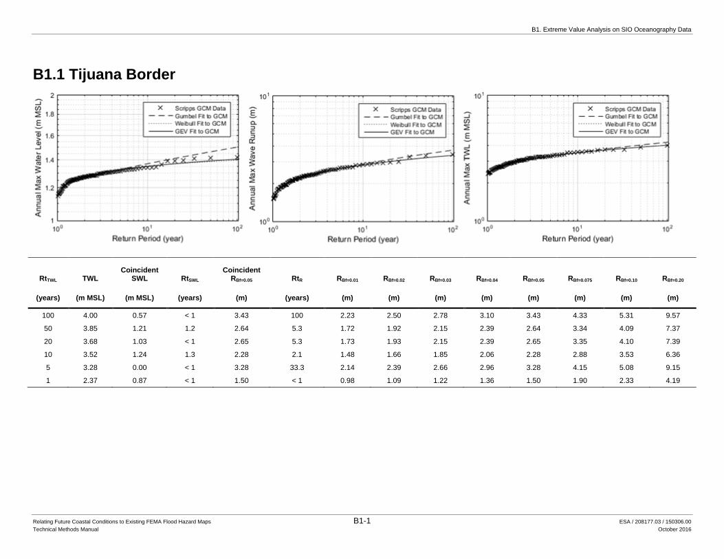
B1. Extreme Value Analysis on SIO Oceanography Data
Relating Future Coastal Conditions to Existing FEMA Flood Hazard Maps B1-1 ESA / 208177.03 / 150306.00
Technical Methods Manual October 2016
B1.1 Tijuana Border
RtTWL TWL Coincident
SWL RtSWL Coincident
RBf=0.05 RtR RBf=0.01 RBf=0.02 RBf=0.03 RBf=0.04 RBf=0.05 RBf=0.075 RBf=0.10 RBf=0.20
(years) (m MSL) (m MSL) (years) (m) (years) (m) (m) (m) (m) (m) (m) (m) (m)
100 4.00 0.57 < 1 3.43 100 2.23 2.50 2.78 3.10 3.43 4.33 5.31 9.57
50 3.85 1.21 1.2 2.64 5.3 1.72 1.92 2.15 2.39 2.64 3.34 4.09 7.37
20 3.68 1.03 < 1 2.65 5.3 1.73 1.93 2.15 2.39 2.65 3.35 4.10 7.39
10 3.52 1.24 1.3 2.28 2.1 1.48 1.66 1.85 2.06 2.28 2.88 3.53 6.36
5 3.28 0.00 < 1 3.28 33.3 2.14 2.39 2.66 2.96 3.28 4.15 5.08 9.15
1 2.37 0.87 < 1 1.50 < 1 0.98 1.09 1.22 1.36 1.50 1.90 2.33 4.19
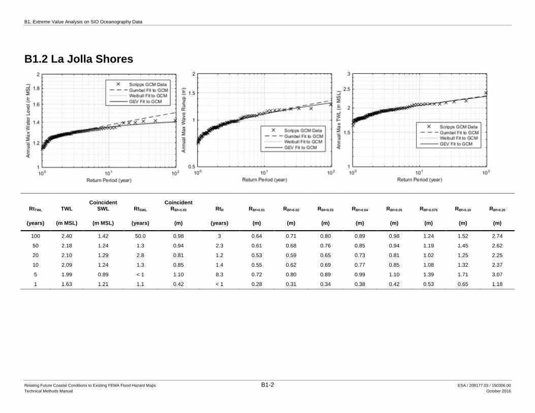
B1. Extreme Value Analysis on SIO Oceanography Data
Relating Future Coastal Conditions to Existing FEMA Flood Hazard Maps B1-2 ESA / 208177.03 / 150306.00
Technical Methods Manual October 2016
B1.2 La Jolla Shores
RtTWL TWL Coincident
SWL RtSWL Coincident
RBf=0.05 RtR RBf=0.01 RBf=0.02 RBf=0.03 RBf=0.04 RBf=0.05 RBf=0.075 RBf=0.10 RBf=0.20
(years) (m MSL) (m MSL) (years) (m) (years) (m) (m) (m) (m) (m) (m) (m) (m)
100 2.40 1.42 50.0 0.98 3 0.64 0.71 0.80 0.89 0.98 1.24 1.52 2.74
50 2.18 1.24 1.3 0.94 2.3 0.61 0.68 0.76 0.85 0.94 1.19 1.45 2.62
20 2.10 1.29 2.8 0.81 1.2 0.53 0.59 0.65 0.73 0.81 1.02 1.25 2.25
10 2.09 1.24 1.3 0.85 1.4 0.55 0.62 0.69 0.77 0.85 1.08 1.32 2.37
5 1.99 0.89 < 1 1.10 8.3 0.72 0.80 0.89 0.99 1.10 1.39 1.71 3.07
1 1.63 1.21 1.1 0.42 < 1 0.28 0.31 0.34 0.38 0.42 0.53 0.65 1.18
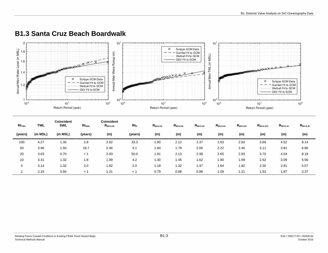
B1. Extreme Value Analysis on SIO Oceanography Data
Relating Future Coastal Conditions to Existing FEMA Flood Hazard Maps B1-3 ESA / 208177.03 / 150306.00
Technical Methods Manual October 2016
B1.3 Santa Cruz Beach Boardwalk
RtTWL TWL Coincident
SWL RtSWL Coincident
RBf=0.05 RtR RBf=0.01 RBf=0.02 RBf=0.03 RBf=0.04 RBf=0.05 RBf=0.075 RBf=0.10 RBf=0.20
(years) (m MSL) (m MSL) (years) (m) (years) (m) (m) (m) (m) (m) (m) (m) (m)
100 4.27 1.35 2.8 2.92 33.3 1.90 2.12 2.37 2.63 2.92 3.69 4.52 8.14
50 3.96 1.50 16.7 2.46 9.1 1.60 1.79 2.00 2.22 2.46 3.11 3.81 6.86
20 3.63 0.70 < 1 2.93 50.0 1.91 2.13 2.38 2.65 2.93 3.70 4.54 8.18
10 3.31 1.32 1.8 1.99 4.2 1.30 1.45 1.62 1.80 1.99 2.52 3.09 5.56
5 3.14 1.32 2.0 1.82 2.0 1.18 1.32 1.47 1.64 1.82 2.30 2.81 5.07
1 2.15 0.94 < 1 1.21 < 1 0.79 0.88 0.98 1.09 1.21 1.53 1.87 3.37
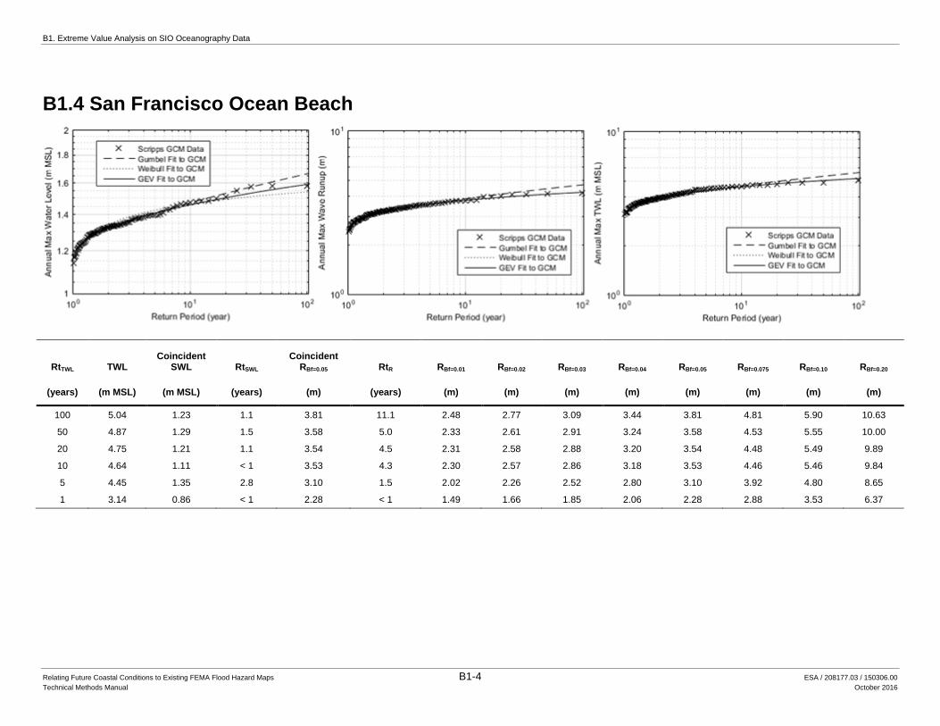
B1. Extreme Value Analysis on SIO Oceanography Data
Relating Future Coastal Conditions to Existing FEMA Flood Hazard Maps B1-4 ESA / 208177.03 / 150306.00
Technical Methods Manual October 2016
B1.4 San Francisco Ocean Beach
RtTWL TWL Coincident
SWL RtSWL Coincident
RBf=0.05 RtR RBf=0.01 RBf=0.02 RBf=0.03 RBf=0.04 RBf=0.05 RBf=0.075 RBf=0.10 RBf=0.20
(years) (m MSL) (m MSL) (years) (m) (years) (m) (m) (m) (m) (m) (m) (m) (m)
100 5.04 1.23 1.1 3.81 11.1 2.48 2.77 3.09 3.44 3.81 4.81 5.90 10.63
50 4.87 1.29 1.5 3.58 5.0 2.33 2.61 2.91 3.24 3.58 4.53 5.55 10.00
20 4.75 1.21 1.1 3.54 4.5 2.31 2.58 2.88 3.20 3.54 4.48 5.49 9.89
10 4.64 1.11 < 1 3.53 4.3 2.30 2.57 2.86 3.18 3.53 4.46 5.46 9.84
5 4.45 1.35 2.8 3.10 1.5 2.02 2.26 2.52 2.80 3.10 3.92 4.80 8.65
1 3.14 0.86 < 1 2.28 < 1 1.49 1.66 1.85 2.06 2.28 2.88 3.53 6.37
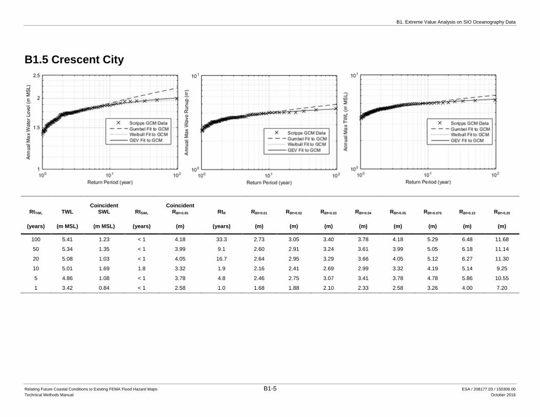
B1. Extreme Value Analysis on SIO Oceanography Data
Relating Future Coastal Conditions to Existing FEMA Flood Hazard Maps B1-5 ESA / 208177.03 / 150306.00
Technical Methods Manual October 2016
B1.5 Crescent City
RtTWL TWL Coincident
SWL RtSWL Coincident
RBf=0.05 RtR RBf=0.01 RBf=0.02 RBf=0.03 RBf=0.04 RBf=0.05 RBf=0.075 RBf=0.10 RBf=0.20
(years) (m MSL) (m MSL) (years) (m) (years) (m) (m) (m) (m) (m) (m) (m) (m)
100 5.41 1.23 < 1 4.18 33.3 2.73 3.05 3.40 3.78 4.18 5.29 6.48 11.68
50 5.34 1.35 < 1 3.99 9.1 2.60 2.91 3.24 3.61 3.99 5.05 6.18 11.14
20 5.08 1.03 < 1 4.05 16.7 2.64 2.95 3.29 3.66 4.05 5.12 6.27 11.30
10 5.01 1.69 1.8 3.32 1.9 2.16 2.41 2.69 2.99 3.32 4.19 5.14 9.25
5 4.86 1.08 < 1 3.78 4.8 2.46 2.75 3.07 3.41 3.78 4.78 5.86 10.55
1 3.42 0.84 < 1 2.58 1.0 1.68 1.88 2.10 2.33 2.58 3.26 4.00 7.20
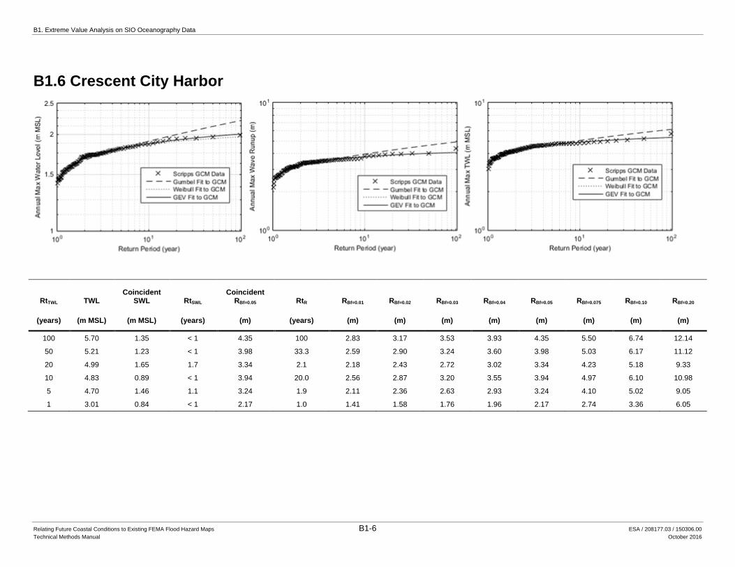
B1. Extreme Value Analysis on SIO Oceanography Data
Relating Future Coastal Conditions to Existing FEMA Flood Hazard Maps B1-6 ESA / 208177.03 / 150306.00
Technical Methods Manual October 2016
B1.6 Crescent City Harbor
RtTWL TWL Coincident
SWL RtSWL Coincident
RBf=0.05 RtR RBf=0.01 RBf=0.02 RBf=0.03 RBf=0.04 RBf=0.05 RBf=0.075 RBf=0.10 RBf=0.20
(years) (m MSL) (m MSL) (years) (m) (years) (m) (m) (m) (m) (m) (m) (m) (m)
100 5.70 1.35 < 1 4.35 100 2.83 3.17 3.53 3.93 4.35 5.50 6.74 12.14
50 5.21 1.23 < 1 3.98 33.3 2.59 2.90 3.24 3.60 3.98 5.03 6.17 11.12
20 4.99 1.65 1.7 3.34 2.1 2.18 2.43 2.72 3.02 3.34 4.23 5.18 9.33
10 4.83 0.89 < 1 3.94 20.0 2.56 2.87 3.20 3.55 3.94 4.97 6.10 10.98
5 4.70 1.46 1.1 3.24 1.9 2.11 2.36 2.63 2.93 3.24 4.10 5.02 9.05
1 3.01 0.84 < 1 2.17 1.0 1.41 1.58 1.76 1.96 2.17 2.74 3.36 6.05
Relating Future Coastal Conditions to Existing FEMA Flood Hazard Maps B2-1 ESA / 208177.03 / 150306.00
Technical Methods Manual October 2016
APPENDIX B2
Extreme Value Analysis on Observed Data
An extreme value analysis was conducted using observed data for three locations along the
California Coast:
Tijuana Border (with La Jolla tides)
San Francisco Ocean Beach
Crescent City
Runup:
Stockdon = Bf=0.05
Modified TAW Bf=0.05; backshore slope m=0.25
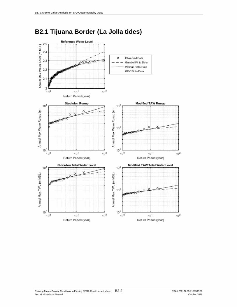
B1. Extreme Value Analysis on SIO Oceanography Data
Relating Future Coastal Conditions to Existing FEMA Flood Hazard Maps B2-2 ESA / 208177.03 / 150306.00
Technical Methods Manual October 2016
B2.1 Tijuana Border (La Jolla tides)
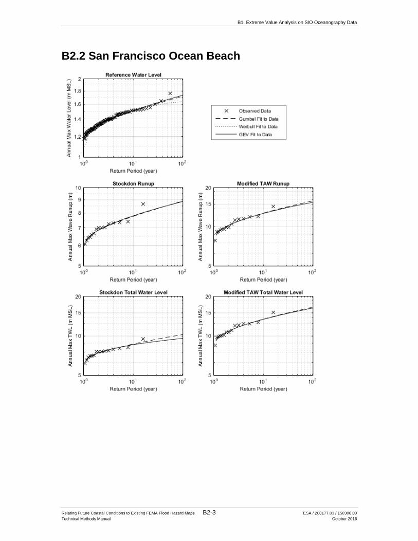
B1. Extreme Value Analysis on SIO Oceanography Data
Relating Future Coastal Conditions to Existing FEMA Flood Hazard Maps B2-3 ESA / 208177.03 / 150306.00
Technical Methods Manual October 2016
B2.2 San Francisco Ocean Beach
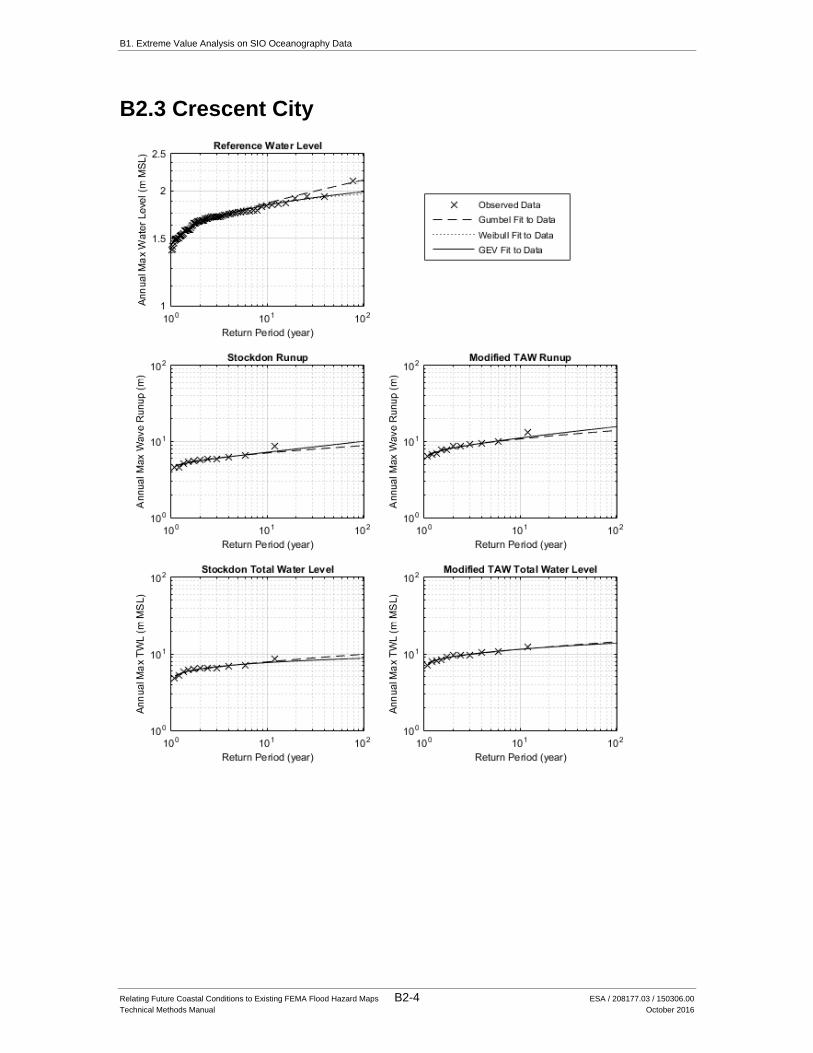
B1. Extreme Value Analysis on SIO Oceanography Data
Relating Future Coastal Conditions to Existing FEMA Flood Hazard Maps B2-4 ESA / 208177.03 / 150306.00
Technical Methods Manual October 2016
B2.3 Crescent City
B1. Extreme Value Analysis on SIO Oceanography Data
Relating Future Coastal Conditions to Existing FEMA Flood Hazard Maps B2-5 ESA / 208177.03 / 150306.00
Technical Methods Manual October 2016
This page intentionally left blank

Relating Future Coastal Conditions to Existing FEMA Flood Hazard Maps C-1 ESA / 208177.03 / 150306.00
Technical Methods Manual October 2016
APPENDIX C
Other Sea Level Rise Hazard Mapping Studies and Sources
The purpose of this Appendix is to identify and describe available projections of future coastal
hazards that might be used for local planning, and to clarify the differences sufficiently to support
a selection by a potential user of this Manual. There are multiple sea level rise hazard studies and
map viewers for the California Coast. California has also produced policy guidance including
selection of sea level rise projections and methods / guidelines. Less information is presently
available for other states. The US Army Corps of Engineers has also developed guidance for projects
which they participate in. Local guidance has been developed to varying levels of completion
with guidance by the City and County of San Francisco being one of the more advanced.
The State of California has also developed Tsunami Maps, which show the potential extents of an
extreme tsunami of undefined recurrence interval. These maps show inundation on a fixed
geometry and do not consider erosion or scour specifically. Tsunami mapping is not addressed in
this Technical Manual.
Future coastal hazards are being addressed via multiple endeavors at all levels of government and
including non-government organizations such as The Nature Conservancy. There is a general
recognition of the need to relate future conditions hazards to existing FEMA maps. This need is
particularly acute at the local level.
There are three leading coastal hazard mapping methodologies being applied in California: the
CoSMoS methodology developed by the United States Geologic Survey (USGS), the ESA PWA
methodology developed for the State of California, and the SPAWAR and TerraCosta
methodology developed for the US Navy. These three are briefly described in Sections C.1
through C.3, respectively. It should be noted that these methodologies are not independent
because each has some level of collaboration with the others. For example, Scripps Institution of
Oceanography (SIO) has provided future water levels and wave conditions, and the Coastal Data
Information Program (CDIP) has provided wave transformation results. The USGS has provided
historical shore positions, erosion rates and seafloor mapping. Much of the work relies on
mapping funded by the State of California.
Section C.4 identifies a few other resources that are often cited but are relatively limited in their
technical basis or geographical extent. There have been several reviews of future coastal
modeling methodologies with a focus of determining differences and appropriate uses. An
example comparison is shown in Table C.1.
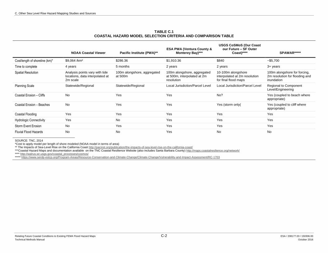
C. Other Sea Level Rise Hazard Mapping Studies and Sources
Relating Future Coastal Conditions to Existing FEMA Flood Hazard Maps C-2 ESA / 208177.03 / 150306.00
Technical Methods Manual October 2016
TABLE C.1 COASTAL HAZARD MODEL SELECTION CRITERIA AND COMPARISON TABLE
NOAA Coastal Viewer Pacific Institute (PWA)** ESA PWA (Ventura County &
Monterey Bay)***
USGS CoSMoS (Our Coast our Future – SF Outer
Coast)**** SPAWAR*****
Cost/length of shoreline (km)* $9,064 /km² $286.36 $1,910.36 $840 ~$5,700
Time to complete 4 years 5 months 2 years 2 years 3+ years
Spatial Resolution Analysis points vary with tide locations, data interpolated at 2m scale
100m alongshore, aggregated at 500m
100m alongshore, aggregated at 500m, interpolated at 2m resolution
10-100m alongshore interpolated at 2m resolution for final flood maps
100m alongshore for forcing, 2m resolution for flooding and inundation
Planning Scale Statewide/Regional Statewide/Regional Local Jurisdiction/Parcel Level Local Jurisdiction/Parcel Level Regional to Component Level/Engineering
Coastal Erosion – Cliffs No Yes Yes No? Yes (coupled to beach where appropriate)
Coastal Erosion – Beaches No Yes Yes Yes (storm only( Yes (coupled to cliff where appropriate)
Coastal Flooding Yes Yes Yes Yes Yes
Hydrologic Connectivity Yes No Yes Yes Yes
Storm Event Erosion No Yes Yes Yes Yes
Fluvial Flood Hazards No No Yes No No
SOURCE: TNC, 2014 *Cost to apply model per length of shore modeled (NOAA model in terms of area) ** The Impacts of Sea-Level Rise on the California Coast http://pacinst.org/publication/the-impacts-of-sea-level-rise-on-the-california-coast/ ***Coastal Hazard Maps and documentation available on the TNC Coastal Resilience Website (also includes Santa Barbara County) http://maps.coastalresilience.org/network/ **** http://walrus.wr.usgs.gov/coastal_processes/cosmos/ ***** https://www.serdp-estcp.org/Program-Areas/Resource-Conservation-and-Climate-Change/Climate-Change/Vulnerability-and-Impact-Assessment/RC-1703
C. Other Sea Level Rise Hazard Mapping Studies and Sources
Relating Future Coastal Conditions to Existing FEMA Flood Hazard Maps C-3 ESA / 208177.03 / 150306.00
Technical Methods Manual October 2016
The State of California has funded a study of coastal hazards in Los Angeles County as a
collaboration between the three primary methodologies, while communities are proceeding with
local coastal planning using available information (See Section C.2.a Los Angeles County).
C.1 CoSMoS – United States Geologic Survey
The Coastal Storm Modeling System (CoSMoS) has been developed to project future coastal
hazards associated with climate change, and has been applied in central and southern California
by the United States Geological Survey (USGS)50. CoSMoS has undergone several refinements,
called 1.0 (southern California circa 201051), 2.0 (central California circa 2012 within a program
called Our Coast Our Future (OCOF)52), 2.1 (San Francisco Bay circa 2014 within a program
called Our Coast Our Future (OCOF)53) and 3.0 (southern California update, initial results
available circa 2015)54,55.
CoSMoS is a methodology comprised of a series of models driven by future predictions derived
from downscaled Global Climate Models (GCMs). The downscaled GCM data are used to
develop water level and wave time series that are used to develop nearshore wave conditions and
flooding projections. These results are combined with existing and historical shore and erosion
data to drive models of shore response and projected future erosion hazards. Earlier versions (e.g.
1.0 and 2.0) focused on coastal flooding and storm erosion but did not include climate-driven,
long-term erosion.
CoSMoS 1.0 – Southern California
The first application was to the southern California bight from Point Conception to the Mexican
border. The study was a collaboration with Deltares, a Dutch quasigovernment organization, and
several other US organizations. This application focused on storm conditions with a range of
higher sea levels. Additional information is available at public websites and in peer-reviewed
publications56 57.
CoSMoS 2.0 – North-central California, Our Coast Our Future
Coastal Storm Modeling System (CoSMoS) was upgraded to the second version as part of an
application for the north-central California coast from Bodega Bay (Sonoma County) to Half
Moon Bay (San Mateo County58 59). This application was a collaboration with the National
50 Barnard, P.L., van Ormondt, M., Erikson, L.H., Eshleman, J., Hapke, C., Ruggiero, P., Adams, P.N. and Foxgrover,
A.C., 2014 (accepted). Development of the Coastal Storm Modeling System (CoSMoS) for predicting the impact of storms on high-energy, active-margin coasts. Natural Hazards. http://dx.doi.org/10.1007/s11069-014-1236-y
51 http://cosmos.deltares.nl/SoCalCoastalHazards/index.html 52 http://data.prbo.org/apps/ocof/ 53 http://data.prbo.org/apps/ocof/ 54 https://walrus.wr.usgs.gov/coastal_processes/cosmos/ 55 https://www.sciencebase.gov/catalog/item/5633fea2e4b048076347f1cf 56 http://cosmos.deltares.nl/SoCalCoastalHazards/index.html 57 Barnard, P.L., van Ormondt, M., Erikson, L.H., Eshleman, J., Hapke, C., Ruggiero, P., Adams, P. N., and
Foxgrover, A. 2014. Coastal Storm Modeling System: CoSMoS. Southern California 1.0, projected flooding hazards, http://walrus.wr.usgs.gov/coastal_processes/cosmos/socal1.0/ , doi:10.5066/F74B2ZB4
58 http://data.prbo.org/apps/ocof/ 59 http://data.prbo.org/apps/ocof/index.php?page=flood-map
C. Other Sea Level Rise Hazard Mapping Studies and Sources
Relating Future Coastal Conditions to Existing FEMA Flood Hazard Maps C-4 ESA / 208177.03 / 150306.00
Technical Methods Manual October 2016
Oceanographic and Atmospheric Administration (NOAA), including the NOAA marine
sanctuaries in the study area, as well as the non-government organization Point Blue
Conservation Science (formerly Point Reyes Bird Observatory) and others. A web-based
interactive viewer allows visualization of projected extents of flood and erosion hazards for a
range of sea level rises and storm recurrence intervals. The hazards mapped are future limits of
inundation by high ocean water levels and wave runup , and shore changes due to storm erosion
and the projection of historical shore erosion rates into the future. Future erosion due to sea level
rise is not included, and long term erosion is not considered in coastal flood projections. Some
coastal structures are modeled as “non-erodible” and therefore implicitly presumed to withstand
all existing and future conditions.
CoSMoS 2.1 – San Francisco Bay, Our Coast Our Future
CoSMoS 2.0 was modified to version 2.1 for application to San Francisco Bay with an emphasis
of tidal hydrodynamics and wind fields for the estuary60. This project was an extension of the Our
Coast Our Future (OCOF) collaboration. Results are combined and accesses via the OCOF
website61 .
CoSMoS 2.2 – South-northern California, Our Coast Our Future
As part of OCOF, CoSMoS is extended north of Bodega Bay to Point Arena. Upgrades to the 2.0
version entail consideration of major river estuaries such as the Russian River mouth.
CoSMoS 3.0– Southern California
The prior southern California mapping (CoSMoS 1.0) is being updated with partial, preliminary
results made available in 201562 63. This version is the first to include new methods for
computing climate-driven (sea level rise) erosion for beaches and cliffs.
C.2 State of California - ESA-PWA
First Generation – State Wide - Pacific Institute
The Pacific Institute maps were produced with funding from the State of California to inform a
state-side assessment of vulnerability to climate change64,65. These maps show future coastal
flood and erosion hazards with sea level rise for several time periods and the Interim Guidance
60 http://data.prbo.org/apps/ocof/ 61 http://data.prbo.org/apps/ocof/index.php?page=flood-map 62 Barnard, P.L., van Ormondt, M., Erikson, L.H., Eshleman, J., Hapke, C., Ruggiero, P., Adams, P.N. and Foxgrover,
A.C., 2014 (accepted). Development of the Coastal Storm Modeling System (CoSMoS) for predicting the impact of storms on high-energy, active-margin coasts. Natural Hazards. http://dx.doi.org/10.1007/s11069-014-1236-y
63 https://www.sciencebase.gov/catalog/item/5633fea2e4b048076347f1cf 64 CEC, 2009; THE IMPACTS OF SEA-LEVEL RISE ON THE CALIFORNIA COAST A Paper From: California
Climate Change Center. Prepared By: Matthew Heberger, Heather Cooley, Pablo Herrera, Peter H. Gleick, and Eli Moore of the Pacific Institute http://www.energy.ca.gov/publications/displayOneReport.php?pubNum=CEC-500-2009-024-F
65 PWA, 2009; California Coastal Erosion Response to Sea Level Rise and Mapping, Prepared for the Pacific Institute, Prepared by Philip Williams & Associates, Ltd., March 11,2009, PWA Project 1939. http://www.esassoc.com/sites/default/files/PWA_OPC_Methods_final.pdf
C. Other Sea Level Rise Hazard Mapping Studies and Sources
Relating Future Coastal Conditions to Existing FEMA Flood Hazard Maps C-5 ESA / 208177.03 / 150306.00
Technical Methods Manual October 2016
for sea level rise (i.e. 1.4 meters by 2100)66. The maps are available from the Pacific Institute67 .
The work was peer-reviewed by the Ocean Science Trust (OST, affiliated with the California
Ocean Protection Council), and there are several peer-reviewed publications68, 69,70. These were
the first maps to project future coastal erosion due to accelerated sea level rise. The
hydrodynamic and geomorphic work was accomplished by PWA (now ESA) for the Pacific
Coast and the USGS model results were used for the SF Bay71. There were several other key
study partners including Scripps (future water level and wave time series for 100 years) and the
Coastal Data Information Program (CDIP; provided regional wave transformations). The hazard
analysis was conducted to inform California’s assessment of vulnerability to climate change and
the adaptation strategy, and greatly expanded the perception of coastal hazards associated with
sea level rise to locations above and landward of future sea levels. Subsequent work has
reinforced that accelerated erosion due to accelerated sea level rise is both important for planning
but inherently uncertain given available methods and data. One aspect of the study that has been
largely overlooked is that it developed estimates of the 100-year wave runup elevation for the
entire California coast, most of which was not mapped by FEMA at the time. The coastal flood
maps are known to overstate the potential for wave-induced flooding in back barrier areas due to
the projection of wave runup elevations that were computed for the coastal barriers (ie. dunes).
This study is a “first generation” study (circa 2008) with updated methods and results for several
regions (i.e. Ventura County, Monterey Bay – Santa Cruz County, and Santa Barbara County) as
described in the “Second Generation” mapping.
Second Generation, Selected Counties – ESA
The State of California and The Nature Conservancy (TNC) funded refined mapping for coastal
zone planning purposes. This mapping is a refined version of the Pacific Institute mapping, and is
called “second generation” in this report. Refinements included revised bluff erosion and flooding
methods, stepwise projection of flooding on eroded shore projections, and were applied for
multiple sea level rise scenarios (typically three; High, Medium and Low) and multiple time-
horizons (typically existing, 2030, 2060 and 2100). These studies developed for planning at
66 http://www.slc.ca.gov/Sea_Level_Rise/SLR_Guidance_Document_SAT_Responses.pdf 67 http://www2.pacinst.org/reports/sea_level_rise/hazmaps.html 68 Heberger et al, 2011; J Climatic Change, V 109, N 1, R 10.1007/s10584-011-0308-1, The Potential impacts of
increased coastal flooding in California due to sea-level rise , Springer Netherlands, 2011-12-01, Heberger, Matthew; Cooley, Heather; Herrera, Pablo; Gleick, Peter H.; Moore, Eli; 229-249, http://dx.doi.org/10.1007/s10584-011-0308-1 ,http://link.springer.com/article/10.1007/s10584-011-0308-1
69 Revell et al, 2011. Revell, D.L., Battalio, B., Spear, B., Ruggiero, P, and Vandever, J. A Methodology for Predicting Future Coastal Hazards due to Sea level Rise on the California Coast. Journal of Climatic Change (2011) B.V. 2011 109 (Suppl 1):S251–S276, DOI 10.1007/s10584-011-0315-2, 10 December 2011 # Springer Science+Business Media http://dx.doi.org/10.1007/s10584-011-0315-2 http://link.springer.com/article/10.1007%2Fs10584-011-0315-2
70 Bromirski, P. D., D. R. Cayan, N. Graham, R. E. Flick, and M. Tyree (Scripps Institution of Oceanography). 2012. Coastal Flooding Potential Projections: 2000–2100. California Energy Commission. CEC‐ 500‐ 2012‐ 011.
71 Knowles, N. 2008. Potential Inundation due to Rising Sea Levels in the San Francisco Bay; http://escholarship.org/uc/item/8ck5h3qn Region. A report from the California Climate Change Center, sponsored by the California Energy Commission and the California Environmental Protection Agency, Sacramento, CA. CEC-500-2009-023-F.
C. Other Sea Level Rise Hazard Mapping Studies and Sources
Relating Future Coastal Conditions to Existing FEMA Flood Hazard Maps C-6 ESA / 208177.03 / 150306.00
Technical Methods Manual October 2016
higher resolution using updated methods are available for Ventura County72, Monterey Bay73
and Santa Barbara County74. These reports and map files are available for download on the
Coastal Resilience website of The Nature Conservancy (TNC), which also includes an interactive
viewer75 . Coastal flooding and erosion are mapped for a range of future sea level rise amounts
through the year 2100, including erosion of sandy and rocky shores with accelerated sea level
rise, and back-barrier flooding. Riverine flooding is also included major streams, using future
precipitation changes from downscaled climate model output. A similar application for Los
Angeles County is underway.
Third Generation
The State of California has funded additional hazard mapping to inform coastal planning, and this
work is ongoing at the time of this report.
(a) Two Line Shore Response Model - ESA
Using State of California “Climate Ready” grant funds, ESA has developed a refined shore
response model that can accommodate a range of adaptation strategies along with the
coastal flood and erosion hazards for the range of sea level rise scenarios. Adaptation
scenarios that can be modeled include coastal armoring and beach nourishment, and predict
resulting beach location and width. This “Third Generation” hazard mapping accounts for
both the shore line and backshore line, and is hence called a “two-line model” of shore
evolution. The application was for southern Monterey Bay for sandy shores in support of a
study called Economic Impacts of Climate Adaptation Strategies in Southern Monterey Bay
led by The Nature Conservancy and involving a team of scientists and ESA76. This two-
line erosion model was also applied on behalf of the US Army Corps of Engineers for the
San Francisco-Daly City-Pacifica, California shore, which includes bluff-backed shores
with narrow beaches77.
(b) CoSMoS 3.0 USGS
The USGS is applying the newest version of their modeling system called CoSMoS 3.0 for
southern California, as described in Section C.1. CoSMoS 3.0.
(c) Los Angeles County – AdaptLA
72 ESA PWA (2013), COASTAL RESILIENCE VENTURA, Technical Report for Coastal Hazards Mapping,
Prepared for The Nature Conservancy, July 31, 2013, ESA PWA project number D211452.00. 73 ESA PWA (2014), MONTEREY BAY SEA LEVEL RISE VULNERABILITY ASSESSMENT, Technical
Methods Report, Prepared for The Monterey Bay Sanctuary Foundation, June 16, 2014. ESA PWA project number D211906.00.
74 ESA (2015), SANTA BARBARA COUNTY COASTAL HAZARD MODELING AND VULNERABILITY ASSESSMENT, Technical Report for Coastal Hazards Mapping, Prepared for the County of Santa Barbara, August 3, 2015, ESA project number D130526.
75 http://maps.coastalresilience.org/california/# - select location and then select viewer, download data or technical report.
76 ESA (2015), Shore Modeling Methodology, Monterey Coastal Adaptation Physical and Economics Modeling, SCC Climate Ready Grant, ESA project 130604.00, Draft - December, 2015.
77 ESA (2015), SAN FRANCISCO LITTORAL CELL, Coastal Regional Sediment Management Plan Draft, Prepared for U.S. Army Corp of Engineers and the Coastal Sediment Management Workgroup, ESA Project 211658, August 2015
C. Other Sea Level Rise Hazard Mapping Studies and Sources
Relating Future Coastal Conditions to Existing FEMA Flood Hazard Maps C-7 ESA / 208177.03 / 150306.00
Technical Methods Manual October 2016
Coastal hazards are being mapped in Los Angeles County under the coastal zone planning
program called AdaptLA78 which is a consortium of Los Angeles County, Cities in the
county, and non-government organizations. This mapping entails a coordinated effort with
modeling by several consultants (ESA and TerraCosta) and the USGS. The hazard mapping
will be derived using the results from several methodologies and will also provide an
opportunity to assess the method differences and range of results as a measure of
uncertainty. ESA’s approach will be an extension of prior modeling described in this
section. TerraCosta’s approach is an extension of work accomplished by Scripps Institution
of Oceanography team for the Department of Defense (see Section C.3 SPAWAR Hazard
Mapping – San Diego Naval Facilities - TerraCosta).
C.3 SPAWAR Hazard Mapping – San Diego Naval Facilities - TerraCosta
The United States Navy, Department of Defense, Space and Naval Warfare Systems Command
(SPAWAR) investigated methodologies for assessing vulnerability of naval facilities to sea level
rise. A recent study developed and applied hazard modeling for the Naval Base Coronado (NBC)
and Marine Corps Base Camp Pendleton (MCBCP) Navy/Scripps model as applied to Naval Base
Coronado in San Diego County, CA 79 . The detailed study used research and development by
staff at the Scripps Institution of Oceanography to assess future hazards80 81 82. The methods
consider beach profile response to ocean conditions and also project bluff erosion into the future.
This comprehensive study results in a methodology that can be applied in other California
locations to provide actionable forecasts of future coastal conditions given climate change
scenarios.
C.4 Other
Three are several other resources that project coastal hazards with future conditions. These other
resources are not emphasized in this Manual because they do not include wave action or coastal
changes (erosion), they are focused on a limited area, or more contemporary resources are
available.
NOAA Coastal Viewer and Climate Central’s Surging Seas
The National Oceanographic and Atmospheric Administration (NOAA) developed a internet-based
tool to allow estimates of future inundation with sea level rise, called the “Coastal Viewer” 83 .
78 http://www.adapt.la/ 79 SPAWAR, 2014. A Methodology for Assessing the Impact of Sea Level Rise on Representative Military
Installations in the Southwestern United States (RC-1703), Submitted to the Strategic Environmental Research Program by Dr. Cart Chadwick incollaboration with TerraCosta Consultating Group and others, March, 2014. https://www.serdp-estcp.org/content/download/23835/240627/file/RC-1703-FR.pd
80 Young, Flick, O’Reilly, Chadwick, Guza, Crampton, Helly, 2014. Estimating cliff retreat in southern California considering sea level rise using a sand balance approach.
81 Yates, M. L., R. T. Guza, and W. C. O'Reilly (2009), Equilibrium shoreline response: Observations and modeling, J. Geophys. Res., 114, C09014, doi:10.1029/2009JC005359.
82 Yates, ML, Guza, RT, O'Reilly, WC, Hansen, J & Barnard, PL 2011, 'Equilibrium shoreline response of a high wave energy beach' Journal of Geophysical Research C: Oceans, vol 116, no. C04014, pp. 1-13., 10.1029/2010JC006681
83 http://csc.noaa.gov/digitalcoast/tools/slrviewer
C. Other Sea Level Rise Hazard Mapping Studies and Sources
Relating Future Coastal Conditions to Existing FEMA Flood Hazard Maps C-8 ESA / 208177.03 / 150306.00
Technical Methods Manual October 2016
The tool provides inundation for different sea levels using existing elevations . Distinguishes
between hydraulically connected areas and low-lying areas which may flood but do not have
clear surface water connections in the maps used. A sophisticated web-based geospatial interface
facilitates use, with a range of information useful for coastal planning.
A similar tool is available from Climate Central called Surging Seas84.
Humboldt Bay Inundation Maps
Humboldt Bay inundation with future sea level rise was modeled and mapped by Northern
Hydrology and Engineering with funding from the State of California85 86 . The mapping is based
on a hydrodynamic model with a range of sea level rise values added to a range of ocean water
levels (e.g. Mean Higher High Water, the 100-year water level).
San Francisco Bay Sea Level Rise Maps - BCDC and USGS
Inundation maps for San Francisco Bay based on sea level rise for selected dates and water levels
using fixed geography . The flood limits are based on an increase in sea level of 0.5, 1.0 and 1.5
meters of sea level rise by 2100 . The sea level rise values were added to the existing extreme
high water levels and mapped to all areas below those elevations without regard to hydrologic
connection or other future conditions. The elevations and mapping are derived from USGS Sea
Level Rise Maps for San Francisco Bay87 – Knowles: Water levels projected through 2100 with
1.4 meters of sea level rise for San Francisco Bay . A hydrodynamic model was used to simulate
existing and future Bay water levels based on an ocean boundary condition calibrated with
existing conditions and modified to consider sea level rise for future conditions. Extreme high
water levels (e.g. 100-year) were calculated based on existing statistics and merged with the
existing and future water level modeling to develop extreme high water level maps. Waves,
geomorphic responses (e.g. erosion) and potential changes to tidal dynamics were not modeled.
This study informed the BCDC maps (item 6) and Pacific Institute maps of San Francisco Bay
(Item 3).the USGS modeling described in item 7, below .
San Diego Region – California Energy Commission (CEC) and The San Diego Foundation
A focus study on the San Diego Region was conducted by a team lead by the University of
California, San Diego 88with the support of The San Diego Foundation in order to inform the
84 http://sealevel.climatecentral.org/maps 85 Trinity Associates (2015). HUMBOLDT BAY Sea Level Rise Adaptation Planning Project: Phase II Report
Prepared By Aldaron Laird Trinity Associates February 2015 86 Northern Hydrology & Engineering (2014). Preliminary data release for the Humboldt Bay sea level rise
vulnerability assessment: Humboldt Bay sea level rise inundation mapping. Prepared for the California State Coastal Conservancy and the Coastal Ecosystems Institute of Northern California. Prepared by Northern Hydrology & Engineering, McKinleyville, CA, dated 10 April 2014.
87 Knowles, N. 2008. Potential Inundation due to Rising Sea Levels in the San Francisco Bay; Region. http://escholarship.org/uc/item/8ck5h3qn
88 CEC, 2009; CLIMATE CHANGE-RELATED IMPACTS IN THE SAN DIEGO REGION BY 2050, Prepared by University of California, San Diego, and Science Applications International Corporation (SAIC), Published by California Energy Commission (CEC) California Climate Change Center, CEC-500-2009-027-F, August 2009.
C. Other Sea Level Rise Hazard Mapping Studies and Sources
Relating Future Coastal Conditions to Existing FEMA Flood Hazard Maps C-9 ESA / 208177.03 / 150306.00
Technical Methods Manual October 2016
regional plan through the year 2050, called the Regional Focus 2050 Study 89. The study
produced inundation maps for 2050 based on the IPCC 2008 estimates with 5-, 10-, 25-, and 50-
year wave runup events added to the sea levels.
89 The San Diego Foundation, 2008, SAN DIEGO'S CHANGING CLIMATE: A REGIONAL WAKE-UP CALL,
http://www.issuelab.org/resource/san_diego_foundation_regional_focus_2050_study_climate_change_related_impacts_in_the_san_diego_region_by_2050

C. Other Sea Level Rise Hazard Mapping Studies and Sources
Relating Future Coastal Conditions to Existing FEMA Flood Hazard Maps C-10 ESA / 208177.03 / 150306.00
Technical Methods Manual October 2016
This page intentionally left blank
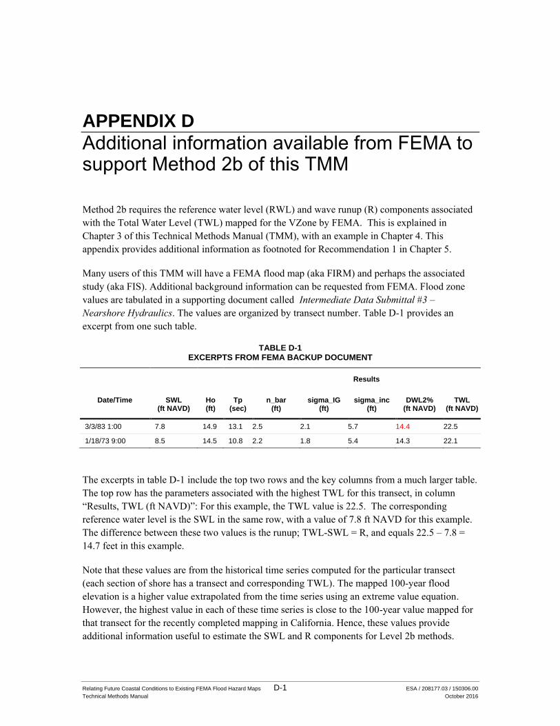
Relating Future Coastal Conditions to Existing FEMA Flood Hazard Maps D-1 ESA / 208177.03 / 150306.00
Technical Methods Manual October 2016
APPENDIX D
Additional information available from FEMA to support Method 2b of this TMM
Method 2b requires the reference water level (RWL) and wave runup (R) components associated
with the Total Water Level (TWL) mapped for the VZone by FEMA. This is explained in
Chapter 3 of this Technical Methods Manual (TMM), with an example in Chapter 4. This
appendix provides additional information as footnoted for Recommendation 1 in Chapter 5.
Many users of this TMM will have a FEMA flood map (aka FIRM) and perhaps the associated
study (aka FIS). Additional background information can be requested from FEMA. Flood zone
values are tabulated in a supporting document called Intermediate Data Submittal #3 –
Nearshore Hydraulics. The values are organized by transect number. Table D-1 provides an
excerpt from one such table.
TABLE D-1 EXCERPTS FROM FEMA BACKUP DOCUMENT
Results
Date/Time SWL (ft NAVD)
Ho (ft)
Tp (sec)
n_bar (ft)
sigma_IG (ft)
sigma_inc (ft)
DWL2% (ft NAVD)
TWL (ft NAVD)
3/3/83 1:00 7.8 14.9 13.1 2.5 2.1 5.7 14.4 22.5
1/18/73 9:00 8.5 14.5 10.8 2.2 1.8 5.4 14.3 22.1
The excerpts in table D-1 include the top two rows and the key columns from a much larger table.
The top row has the parameters associated with the highest TWL for this transect, in column
“Results, TWL (ft NAVD)”: For this example, the TWL value is 22.5. The corresponding
reference water level is the SWL in the same row, with a value of 7.8 ft NAVD for this example.
The difference between these two values is the runup; TWL-SWL = R, and equals 22.5 – 7.8 =
14.7 feet in this example.
Note that these values are from the historical time series computed for the particular transect
(each section of shore has a transect and corresponding TWL). The mapped 100-year flood
elevation is a higher value extrapolated from the time series using an extreme value equation.
However, the highest value in each of these time series is close to the 100-year value mapped for
that transect for the recently completed mapping in California. Hence, these values provide
additional information useful to estimate the SWL and R components for Level 2b methods.
D. Additional Information available from FEMA to support Method 2b of this TMM
Relating Future Coastal Conditions to Existing FEMA Flood Hazard Maps D-2 ESA / 208177.03 / 150306.00
Technical Methods Manual October 2016
This page intentionally left blank


![IOC-SOPAC Regional Workshop on Coastal Global Ocean ... · 3.3 COASTAL GLOBAL OCEAN OBSERVING SYSTEM [Coastal GOOS] The recently completedStrategic Design Plan for the Coastal Component](https://img.pdfslide.us/doc/110x75/5f3f00a1d7baf434065b667f/ioc-sopac-regional-workshop-on-coastal-global-ocean-33-coastal-global-ocean.jpg)