Rejoinder

www.elsevier.com/locate/econbase

Journal of Econometrics 125 (2005) 365–375

Rejoinder

Jeffrey Smitha,*, Petra Toddb

a Department of Economics, University of Maryland, 3105 Tydings Hall, College Park, MD,

20742-7211, USAb Department of Economics, University of Pennsylvania, USA

Available online 17 July 2004

1. Introduction

In this rejoinder, we address the points made in the response by Prof. Dehejia. Ashis response argues that propensity score matching provides a robust solution to theevaluation problem only for the sample employed in the Dehejia and Wahba (hereafter DW) (1999, 2002) papers, we focus our attention on that sample in therejoinder. We argue that, in fact, the evidence from the DW sample clearly showsthat propensity score matching does not solve the evaluation problem in this context.

In Section 2, we clarify the purpose of some of the remarks in the introduction andconclusion of our original paper. In Section 3, we show the sensitivity of biasestimates from single nearest neighbor matching to changes in the experimentalsample (treatment or control) used to estimate the bias, the experimental sample(treatment, control, or both) used to estimate the propensity score, and the choice ofseed for the random number generator used to break ties in the matching. We alsoshow the sensitivity of estimates from kernel matching to the first two factors. InSection 4 we apply three alternative balancing tests to the data, and show that we canreject the balancing condition for the scores employed in the response using thesealternative tests. Section 5 concludes.

2. Dehejia and Wahba (1999, 2002) in the literature

Before turning to the substantive issues raised by the response, a few remarksabout the statements in the introduction and conclusion to our paper regarding the

ARTICLE IN PRESS

*Corresponding author. Tel.: +1-301-405-3532; fax: +1-301-405-3542.

E-mail addresses: [email protected] (J. Smith), [email protected] (P. Todd).

0304-4076/$ - see front matter r 2004 Elsevier B.V. All rights reserved.

doi:10.1016/j.jeconom.2004.04.013

perception in the literature of matching methods in general, and of the DW (1999,2002) papers in particular, are in order. These statements are questioned in Section 2of the response.

These remarks are aimed at the general readership of our paper, and notspecifically at Prof. Dehejia, who makes it clear in his response that he is aware of thelimitations of propensity score matching. Moreover, Prof. Dehejia is correct thatneither of the DW (1999, 2002) papers claim that matching is a magic bullet or that italways solves the evaluation problem. What they do claim is that simple cross-sectional matching methods solve the evaluation problem when applied to the NSWdata, even though the data are weak along several dimensions identified in the earlierliterature (and discussed at length in our paper). Judging by the numerous citationsto the DW (1999, 2002) papers (and their working paper predecessors) in both thepublished and unpublished literature, their findings have contributed strongly to therecent popularity of matching approaches even in weak data contexts, where webelieve such methods are ineffective. Our analysis focused on the DW (1999, 2002)papers, rather than on other papers, precisely because they have been particularlyinfluential in the literature.

3. Does matching solve the selection problem in the NSW data?

Dehejia asserts in his response that matching produces ‘‘reliable and robust’’estimates in the subsample of the Supported Work data utilized in the DW (1999,2002) papers. The evidence reported in this section disputes this claim.

Before presenting the evidence, however, we note that his response still providesno justification for the data subsample used in these two papers. Why wereindividuals with zero earnings in months 13–24 before random assignment who wererandomly assigned after April 1976 included, while individuals with non-zeroearnings in months 13–24 before random assignment who were randomly assignedafter April 1976 were excluded? The response does not address this importantquestion, which we raise in our paper. It seems to us that a researcher starting afreshwith the NSW data would likely choose to use either the whole of LaLonde’s sample,or what we term the early random assignment sample, but would be unlikely to setupon DW’s sample.

We also remark that while we in general agree that different applications willrequire different propensity score specifications, it seems to us worrisome that smallchanges, such as restricting the dates of random assignment in the treated sample orincluding and excluding some observations with zero earnings, should require majorchanges in the propensity score. After all, the same general problem is being solvedfor all three NSW samples—namely, the problem of selection into NSW from eitherthe CPS population or the PSID population.

To examine the sensitivity of propensity score matching applied to the DWsample, we next present 36 alternative estimates of the bias constructed using singlenearest neighbor matching with replacement. Half of the estimates use the CPScomparison group and half of the estimates use the PSID comparison group. For

ARTICLE IN PRESSJ. Smith, P. Todd / Journal of Econometrics 125 (2005) 365–375366

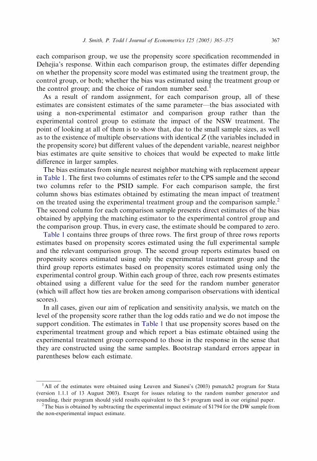
each comparison group, we use the propensity score specification recommended inDehejia’s response. Within each comparison group, the estimates differ dependingon whether the propensity score model was estimated using the treatment group, thecontrol group, or both; whether the bias was estimated using the treatment group orthe control group; and the choice of random number seed.1

As a result of random assignment, for each comparison group, all of theseestimates are consistent estimates of the same parameter—the bias associated withusing a non-experimental estimator and comparison group rather than theexperimental control group to estimate the impact of the NSW treatment. Thepoint of looking at all of them is to show that, due to the small sample sizes, as wellas to the existence of multiple observations with identical Z (the variables included inthe propensity score) but different values of the dependent variable, nearest neighborbias estimates are quite sensitive to choices that would be expected to make littledifference in larger samples.

The bias estimates from single nearest neighbor matching with replacement appearin Table 1. The first two columns of estimates refer to the CPS sample and the secondtwo columns refer to the PSID sample. For each comparison sample, the firstcolumn shows bias estimates obtained by estimating the mean impact of treatmenton the treated using the experimental treatment group and the comparison sample.2

The second column for each comparison sample presents direct estimates of the biasobtained by applying the matching estimator to the experimental control group andthe comparison group. Thus, in every case, the estimate should be compared to zero.

Table 1 contains three groups of three rows. The first group of three rows reportsestimates based on propensity scores estimated using the full experimental sampleand the relevant comparison group. The second group reports estimates based onpropensity scores estimated using only the experimental treatment group and thethird group reports estimates based on propensity scores estimated using only theexperimental control group. Within each group of three, each row presents estimatesobtained using a different value for the seed for the random number generator(which will affect how ties are broken among comparison observations with identicalscores).

In all cases, given our aim of replication and sensitivity analysis, we match on thelevel of the propensity score rather than the log odds ratio and we do not impose thesupport condition. The estimates in Table 1 that use propensity scores based on theexperimental treatment group and which report a bias estimate obtained using theexperimental treatment group correspond to those in the response in the sense thatthey are constructed using the same samples. Bootstrap standard errors appear inparentheses below each estimate.

ARTICLE IN PRESS

1 All of the estimates were obtained using Leuven and Sianesi’s (2003) psmatch2 program for Stata

(version 1.1.1 of 13 August 2003). Except for issues relating to the random number generator and

rounding, their program should yield results equivalent to the S+program used in our original paper.2 The bias is obtained by subtracting the experimental impact estimate of $1794 for the DW sample from

the non-experimental impact estimate.

J. Smith, P. Todd / Journal of Econometrics 125 (2005) 365–375 367

Four major findings emerge from Table 1. First, the numbers in the table bouncearound a lot. The bias estimates for the CPS comparison group vary from $38.67 to$1078.74 in absolute value and those for the PSID comparison group vary from$53.37 to $834.62 in absolute value. This variation likely results from small samplesizes. The DW subset of LaLonde’s sample includes only 185 treatment observationsand 260 control observations. Both the CPS and the PSID comparison groups,despite their large nominal sample sizes, contain only small numbers of observationsfor which the propensity scores are comparable to NSW participants. Furthermore,the dependent variable—earnings in 1978—has a high variance in this population.

The second finding is that using the treatment group to estimate the propensityscores and to estimate the bias, which corresponds to the procedure used to generatethe estimates in Table 2 of the response, yields relatively low bias estimates. For theCPS comparison group, these estimates comprise three of the four smallest (inabsolute value) out of 18. For the PSID comparison group, they are the secondsmallest (in absolute value) out of six.

The third finding is that the bias estimates based on the largest sample sizes—thosethat rely on propensity scores estimated using the full experimental sample andbiases estimated using the experimental control group—are substantial for both

ARTICLE IN PRESS

Table 1

Bias estimates from single nearest neighbor matching with replacment

CPS PSID

Treatment Control Treatment Control

group bias group bias group bias group bias

All experimental observations used for scores

Seed 1 �338.61 (780.88) �665.39 (647.16) 258.51 (1017.54) 708.63 (761.98)

Seed 2 �141.61 (842.02) �679.93 (636.26) 258.51 (894.95) 708.63 (750.19)

Seed 3 �264.16 (814.27) �453.92 (619.02) 258.51 (1007.31) 708.63 (821.09)

Experimental treatment group observations used for scores

Seed 1 �251.84 (734.49) �663.23 (599.36) 74.73 (1053.91) 834.62 (785.86)

Seed 2 38.67 (810.51) �663.15 (633.24) 74.73 (953.48) 834.62 (732.32)

Seed 3 �159.52 (780.72) �586.25 (660.96) 74.73 (1032.67) 834.62 (883.65)

Experimental control group observations used for scores

Seed 1 �1078.74 (810.26) �956.02 (618.53) �53.37 (1139.99) 712.56 (743.24)

Seed 2 �840.99 (810.94) �964.58 (670.01) �53.37 (1054.68) 712.56 (763.20)

Seed 3 �1042.21 (870.13) �777.96 (619.07) �53.57 (1011.56) 712.56 (829.62)

Source: Authors’ calculations using NSW data.

Notes: Seed 1=123456789, Seed 2=987654321 and Seed 3=456789123. All of the estimates are based on

single nearest neighbor matching with replacement using the DW experimental sample. We sort the

observations by their identification number from the LaLonde dataset. No common support condition is

imposed. The experimental impact estimate is $1794. Bootstrap standard errors based on 250 replications

appear in parentheses; these standard errors do not account for the variance component due to estimation

of the scores and, for the treatment group bias estimates, treat the experimental impact as a constant.

J. Smith, P. Todd / Journal of Econometrics 125 (2005) 365–375368

comparison groups. They range between –679.93 and –453.92 for the CPScomparison group and equal 708.63 for the PSID comparison group. In addition,the biases estimated using the experimental control group have smaller estimatedstandard errors due to its larger sample size. These estimates suggest that the verylow bias estimates implicit in Table 2 of the response result from sampling variationin a small sample.

The fourth finding is that the CPS estimates, but not the PSID estimates, are alsosensitive to the particular value selected for the random number seed. The reason forthis is that there exist sets of observations in the combined CPS and experimentalsamples that have exactly the same values of the variables use to calculate thepropensity score (and thus identical estimated propensity scores). For example, inthe pooled treatment group and CPS comparison group sample, there are ten distinctgroups that contain at least one treatment group member and two comparison groupmembers—three of size three, three of size four, three of size six and one of size 10.

To see the trouble this can cause, consider one of the groups with six members.Three of the six are treatment group observations and three are CPS observations.

ARTICLE IN PRESS

Table 2

Bias estimates from kernel matching

Bandwidth CPS PSID




0.09 �1814.69 (588.13) �1506.26 (428.22) �645.31 (866.86) 49.10 (709.60)

0.06 �1813.82 (580.33) �1329.70 (429.25) �568.79 (918.43) 183.99 (721.02)

0.03 �1724.49 (578.66) �1083.50 (415.72) �485.02 (1029.74) 260.38 (814.67)

0.01 �1158.32 (615.84) �680.95 (437.99) �982.91 (1055.17) 296.98 (770.12)

0.005 �898.97 (594.46) �597.62 (476.34) �1345.87 (1013.79) �54.23 (850.13)


0.09 �2134.54 (619.99) �2195.39 (460.86) �424.13 (923.26) 229.11 (727.65)

0.06 �1853.07 (595.63) �1719.77 (428.52) �395.35 (894.16) 428.81 (755.84)

0.03 �1747.12 (596.44) �1410.06 (438.40) �99.47 (929.98) 620.72 (756.41)

0.01 �1354.92 (575.63) �775.73 (423.22) �205.51 (1034.45) 924.28 (864.07)

0.005 �837.55 (573.83) �456.63 (420.71) �636.86 (1171.63) 608.80 (895.62)


0.09 �2018.00 (584.44) �1664.82 (433.38) �1080.86 (1069.11) �234.00 (751.56)

0.06 �1855.71 (593.04) �1540.26 (423.36) �1026.96 (1070.98) �167.37 (781.50)

0.03 �1824.72 (587.81) �1290.92 (422.10) �764.99 (1106.57) 87.66 (775.14)

0.01 �1830.18 (586.22) �886.22 (424.18) �909.08 (1133.66) �172.10 (854.94)

0.005 �1353.11 (619.62) �732.31 (458.59) �1147.93 (1308.36) �838.91 (1007.38)


Notes: All of the estimates are based on kernel matching using the Epanechnikov kernel and the DW

experimental sample. The experimental impact estimate is $1794. Bootstrap standard errors based on 100

replications appear in parentheses; these standard errors do not account for the variance component due

to estimation of the scores and, for the treatment group bias estimates, treat the experimental impact

estimate as a constant.


Although all have the same values for the variables included in the scores—inparticular, they all have zero earnings in ‘‘1974’’ and 1975—the comparisongroup observations have very different earnings in 1978. One earns $12,760, oneearns $4520 and one earns $1956. With single nearest neighbor matching withreplacement, the combined estimated counterfactual earnings for the three treatedobservations in the group can thus range from $38,280 (if all three treatmentgroup members get matched to the comparison observation earning $12,760)down to $5868 (if all three get matched to the comparison observation earning$1956). In a treatment group with only 185 observations, moving from one extremeto the other will change the estimated bias by over $500. Obviously, the presence ofgroups with tied propensity score values introduces a lot of variation into theestimates, and suggests the value of looking at bias estimates based on severaldifferent random sorts of the data, rather than just one, as in the response. Theseproblems also arise when the CPS comparison group is combined with theexperimental control group.

Similar problems with ties in the propensity score values do not arise for the PSIDcomparison group, presumably due to its smaller sample size. As a result, we matchalmost exactly the bias estimate implicit in Table 2 of Dehejia’s response when weuse only the experimental treatment group to estimate the propensity scores and thebias.

To show that the instability of the estimates evident in Table 1 does not resultsolely from the use of single nearest neighbor matching with replacement, we presentestimates based on kernel matching in Table 2. Switching from single nearestneighbor matching to kernel matching trades bias for efficiency, because kernelmatching uses information from less similar observations—those other than thenearest neighbor—but at the same time uses more observations overall inconstructing the estimated counterfactual mean. The efficiency gain can be seen inthe lower estimated standard errors in Table 2 relative to Table 1. The kernelmatching estimates have the virtue that they do not depend on the random numberseed for any of the samples, but the vice that they depend on the choice ofbandwidth. We present estimates obtained using the Epanechnikov kernel and fivewidely spaced bandwidths; we find that, while the estimates have some sensitivity tothe choice of bandwidth, the broader patterns do not.

Two key findings emerge. First, the kernel matching estimates exhibit similar,though not quite as dramatic, sensitivity to whether the treatment group or thecontrol group produces the bias estimate, and to which subset of the experimentalsample is used to estimate the propensity scores. Although the kernel matchingestimates make use of more information from the comparison group sample, they donot change the overall fact that the DW subsample of the NSW data does notcontain very many observations. Second, the kernel matching estimates revealsubstantially larger biases, in general, than the single nearest neighbor matching withreplacement estimates. This finding, which is more negative than the results obtainedusing local linear matching in our paper, provides further evidence in support of ourconclusion that matching does not solve the evaluation problem in the NSW data,even for the DW sample.

ARTICLE IN PRESSJ. Smith, P. Todd / Journal of Econometrics 125 (2005) 365–375370

4. Balancing tests

4.1. The balancing tests we use

As we make clear in our paper, we agree with the remarks in the responseregarding the utility of balancing tests in choosing the specification of the propensityscore model when a parametric model such as a logit or a probit is used to estimatethe scores. At the same time, these tests have a number of limitations. The mostobvious limitation at present is that multiple versions of the balancing test exist inthe literature, with little known about the statistical properties of each one or of howthey compare to one another given particular types of data. DW use a test based onbalancing covariates within intervals but provide no objective way to choose theintervals, which is critical because the power of the test is low for narrow intervals.We consider three different balancing tests in this rejoinder, in part to make the pointthat different tests sometimes yield different answers (particularly in small samples).

The first test we consider comes from Rosenbaum and Rubin (1985) and relies onthe examination of standardized differences. Using the notation in our paper, the

ARTICLE IN PRESS

Table 3

Balancing tests from single nearest neighbor matching with replacement

CPS PSID




Standardized differences 2.12/20.29 1.43/28.40 �1.69/13.12 3.49/16.74

Hotelling test 0.0000 0.0000 0.0014 0.0000

Regression test 3/6/6 4/4/5 6/8/8 9/10/10


Standardized differences �2.08/20.77 �1.26/26.62 �4.29/11.74 �4.62/10.75

Hotelling test 0.0000 0.0000 0.0035 0.0000

Regression test 5/5/6 6/8/9 5/7/9 8/8/9


Standardized differences 1.48/19.80 �1.28/21.30 3.34/15.14 �0.90/10.39

Hotelling test 0.0000 0.0000 0.0012 0.0000

Regression test 3/4/5 4/7/8 7/8/8 9/9/10


Notes: For the standardized differences, the first number is the 5th highest of the 10 standardized

differences corresponding to the 10 variables age, education, no high school degree, black, Hispanic,

married, earnings in ‘‘1974’’, earnings in 1975, no earnings in ‘‘1974’’ and no earnings in 1975. The second

number is the maximum standardized difference. For the regression test, the first number is the number of

p-values below 0.01 for the ten variables, the second the number of p-values below 0.05 and the third the

number of p-values below 0.10. The estimates correspond to Seed 1 in Table 1, values for the other seeds

are qualitatively similar.


standardized difference is defined as

SDIFF ðZkÞ ¼ 100

1

n1

PiAI1

Zki �P

jAI0wði; jÞZkj

h iffiffiffiffiffiffiffiffiffiffiffiffiffiffiffiffiffiffiffiffiffiffiffiffiffiffiffiffiffiffiffiffiffiffiffiffiffiffiffiffiffiffiffiffiffiffiffiffiffiffiffiffivariAI1

ðZkiÞ þ varjAI0ðZkjÞ

2

r :

In words, the standardized difference for a variable Zk is the difference in meansbetween the treated sample and the matched (or, more generally, reweighted)comparison group sample, divided by the square root of the average of the variancesof Zk in the unweighted treatment and comparison groups. Intuitively, thestandardized difference considers the size of the difference in means of aconditioning variable between the treated and matched comparison groups, scaledby the square root of the average of the variances in the original (unweighted)samples. This balancing test has been employed in recent work in economics by,among others, Lechner (1999, 2000) and Sianesi (2002).

A common practice in the literature is to compute the standardized difference forall of the variables included in the matching. Additional power can be obtained byconsidering other moments of these variables and interactions between them,although this is rarely done. We have not been able to find any formal criteria in theliterature for when a standardized bias is too big, though Rosenbaum and Rubin(1985) suggest that a value of 20 is ‘‘large’’. In addition to the lack of formal criteriafor evaluating the size of the standardized bias statistic, the standardized bias test hasthe disadvantage that the researcher can reduce the standardized bias by addingadditional observations to the comparison group, so long as these additionalobservations increase the second variance term in the denominator.

The second balancing test we examine is a Hotelling T2 test of the joint null ofequal means of all of the variables included in the matching between the treatmentgroup and the matched or reweighted comparison group.3 As implemented here,using the command available in Stata, this test is not quite correct because it treatsthe matching weights as fixed rather than random. Whether the test is tooconservative or the reverse depends on the (unknown) covariance between thecomponent of the variance associated with the matching weights and the samplingvariation conditional on the weights.

The third balancing test we employ tests the balancing condition in a regressionframework. In particular, for each variable included in the propensity score, weestimate the following regression:

Zk ¼ b0 þ b1#PðZÞ þ b2

#PðZÞ2

þ b3#PðZÞ3 þ b4

#PðZÞ4 þ b5D þ b6D #PðZÞ

þ b7D #PðZÞ2 þ b8D #PðZÞ3 þ b9D #PðZÞ4 þ Z:

We then test the joint null that the coefficients on all of the terms involving thetreatment dummy equal zero. Essentially, we test whether D provides any

ARTICLE IN PRESS

3 This test was also used in Black and Smith (2004).


information about Zk conditional on a quartic in the estimated propensity score. Ifthe propensity score satisfies the balancing condition, it should not. The downside tothis test is that it requires selection of the order of the polynomial, which may haveimplications for results of the test.

4.2. Evidence on balancing

The results obtained from the three balancing tests described in Section 4.1 appearin Table 3. The test results correspond to the estimates in Table 1 for the first randomnumber seed. The balancing test results for the other two random number seeds withsingle nearest neighbor matching with replacement, and for the kernel matching, arequalitatively similar.

For each combination of comparison group, experimental sample used to estimatethe bias, and experimental sample used to estimate the propensity score, the first rowreports the 5th largest standardized bias out of the 10 variables used in the scores—age, education, no high school degree, black, Hispanic, married, earnings in ‘‘1974’’,zero earnings in ‘‘1974’’, earnings in 1975 and zero earnings in 1975. We also reportthe largest standardized bias among the 10 variables. The second row reports the p-value from the Hotelling T2 test. The third row reports the number of p-values fromthe regression test applied to the 10 variables that were less than 0.01, less than 0.05and less than 0.10.

We highlight three patterns in the test results in Table 3. First, the balancing testsdo fairly poorly, even in the case where both the propensity scores and the bias areestimated using the experimental treatment group, as in the response. In both cases,the Hotelling test rejects balance at the 0.005 level. In both cases, the p-value fromthe regression test is below 0.001 for at least five of the ten variables. In the CPScomparison group, although the 5th largest bias is relatively small, the higheststandardized bias lies above 20, the level characterized as large in Rosenbaum andRubin (1985).

Second, the Hotelling and regression tests suggest imbalance in every casein the table. The maximum standardized biases also suggest concern in most cases,though the 5th largest of the 10 standardized biases often turns out fairly modest.These strong patterns suggest rejecting the propensity score specification that yieldsthe very low biases in Table 2 of Dehejia and Wahba. From this, we conclude notthat balancing tests are useless, but rather that, taking the results here incombination with those in Tables 1 and 2, the samples are small and the estimateshighly variable, so that even poor scores will sometimes yield low biases andapparent balance.

Finally, we note that in several cases the standardized bias test and the othertests suggest different conclusions about balance. This indicates the valueof looking at multiple balancing tests. It also indicates the value of additionalresearch comparing the power of the different tests for particular data generatingprocesses.

ARTICLE IN PRESSJ. Smith, P. Todd / Journal of Econometrics 125 (2005) 365–375 373

5. Conclusions

We believe that the conclusions in our paper continue to hold in light of theevidence presented in the response and in this rejoinder. We add one refinement andone new conclusion.

First, we concluded in our paper that propensity score matching does not solve theselection problem in the NSW data. We believe that the evidence in both theresponse and our rejoinder serves only to strengthen that conclusion. The low biasestimates presented in DW (1999, 2002) and in the response are quite sensitive, notonly in regard to the sample and the propensity score specification as shown in ouroriginal paper, but also to whether the treatment group or the control group (orboth) is used to estimate the propensity score, to whether the bias is estimated usingthe experimental treatment group or the experimental control group and, in the caseof the CPS comparison group, to how ties are broken in single nearest neighbormatching. Moreover, we show in Section 4 that application of standard balancingtests from the literature does not eliminate this sensitivity.4

Second, we add a caution that should be obvious to anyone who looked closely atthe estimated standard errors in either the original DW (1999, 2002) papers or ourpaper, but which we previously emphasized too little. The NSW experimental sampleemployed in LaLonde (1986) is very small, and gets even smaller when subsets suchas the DW sample or the early random assignment sample are considered. Thenumber of useful comparison group observations is also fairly small; the supportanalyses in both DW (1999, 2002) and our paper make this quite clear. The vastmajority of the observations in the CPS comparison sample look nothing likeparticipants in Supported Work. There are more comparable observations in thePSID comparison sample in a relative sense, but that is because it includes a minorityover-sample that is not well documented and for which no weights are available.Small sample sizes mean sensitive results, which is exactly what we document in ourpaper and this response. This does not mean that nothing can be learned from theSupported Work data, only that the results found here should be discountedappropriately and supplemented with findings from larger samples.

Acknowledgements

We thank Dan Black, Michael Lechner, Miana Plesca and Barbara Sianesi forhelpful discussions, Barbara Sianesi and Edwin Leuven for quick responses toquestions about the psmatch2 program and Prof. Dehejia for information about theempirical analyses in his response. We thank the editors of the special issue, JohnHam and Robert LaLonde, for the opportunity to provide this rejoinder and fortheir comments on an earlier version.

ARTICLE IN PRESS

4 Zhong (2003) finds similar sensitivity in his work using the NSW data.


References

Black, D., Smith, J., 2004. How robust is the evidence on the effects of college quality? evidence from

matching. Journal of Econometrics 121, 99–124.

Sianesi, B., 2002. An Evaluation of the Swedish System of Active Labour Market Programmes in the

1990s. Institute for Fiscal Studies Working Paper W02/01.

Zhong, Z., 2003. Data Issues of Using Matching to Estimate Treatment Effects: An Illustration with NSW

Data Set. Unpublished manuscript, Peking University.

ARTICLE IN PRESSJ. Smith, P. Todd / Journal of Econometrics 125 (2005) 365–375 375

Documents

Rejoinder