Rejecting Small Gambles Under Expected Utility∗

Ignacio Palacios-Huerta†

Roberto Serrano‡

Oscar Volij§

First version: April 2001 — This version: April 2004

Abstract

This paper contributes to a recent debate around expected utility and risk aver-sion. Based on introspective rejections of small gambles, expected utility has beendeemed incapable of explaining plausible behavior toward risk. We use empiricalevidence to show that people often accept small gambles. In addition, we show thatrejecting a gamble over a given range of wealth levels imposes a lower bound onrisk aversion. Using this lower bound and empirical evidence on the range of therisk aversion coefficient, we study the relationship between risk attitudes over small-stakes and large-stakes gambles. We find that rejecting small gambles is consistentwith expected utility. Paradoxical behavior is only obtained when the assumptionof rejecting small gambles is made in a region of the parameter space that is notempirically relevant.

JEL Classification: D00, D80, D81.Key Words: Risk Aversion, Expected Utility.

∗We gratefully acknowledge Salomon research awards from Brown University. Serrano also acknowl-edges support from NSF grant SES-0133113, the Alfred P. Sloan Foundation and Deutsche Bank. We areespecially indebted to R. J. Aumann for his invaluable input to the paper. We also thank two anony-mous referees, K. J. Arrow, J. Dubra, J. Green, F. Gul, M. Machina, C. Mulligan, A. Salsbury, L. Stole,R. Vohra, P. Wakker, and participants in the Luncheon Seminar of the School of Social Science at IASin Princeton, the “Rationality on Fridays” Workshop in Jerusalem, and the 2001 CEPR Conference onPsychology and Economics in Brussels for helpful comments. We also acknowledge conversations withM. Rabin and R. Thaler.

†Brown University, ipalacios@brown.edu, http://www.econ.brown.edu/˜iph‡Brown University, roberto serrano@brown.edu, http://www.econ.brown.edu/faculty/serrano§Iowa State University and Ben-Gurion University of the Negev, oscar@volij.co.il, http://www.volij.co.il

“The report of my death was an exaggeration.”

Mark Twain (May 1897)

1 Introduction

The expected utility framework has been severely criticized in a recent literature that

concludes that diminishing marginal utility is an utterly implausible explanation for risk

aversion.1 The basis of the criticism can be best illustrated in Rabin (2000), who studies

the relationship between risk attitudes over small and large stakes gambles under expected

utility. Using his results, it is possible to present striking statements of the following kind:

if a decision maker is a risk-averse expected utility maximizer and if he rejects gambles

involving small stakes over a large range of wealth levels, then he will also reject gambles

involving large stakes, sometimes with infinite positive returns. For instance, “suppose

that, from any initial wealth level, a person turns down gambles where she loses $100 or

gains $110, each with 50% probability. Then she will turn down 50-50 bets of losing $1,000

or gaining any sum of money,” or “suppose we knew a risk averse person turns down 50-50

lose $100 or gain $105 bets for any lifetime wealth level less than $350,000 . . . Then we

know that from an initial wealth level of $340,000 the person will turn down a 50-50 bet

of losing $4,000 and gaining $635,670.” (Rabin, 2000, p. 1282).

From this paradoxical, even absurd, behavior towards large-stakes gambles, Rabin

(2000) and other authors conclude that expected utility is fundamentally unfit to ex-

plain decisions under uncertainty. This paper challenges this conclusion. We show that

the paradoxes identified in this literature have little empirical support.2 In particular, we

show that it is the assumption of rejecting small gambles over a large range of wealth levels,

and not expected utility, that does not typically match real-world behavior. In articulating

our response, it is more useful not to argue whether expected utility is literally true (we

know that it is not, since many violations of its underpinning axioms have been exhibited).

1See, for example, Hansson (1988), Kandel and Stambaugh (1991), Rabin (2001), Rabin and Thaler(2001) and other references therein. Samuelson (1963), Machina (1982), Segal and Spivak (1990) andEpstein (1992) also study various issues that are related to this literature.

2See Watt (2002), who has independently obtained results related to ours.

1

Rather, one should insist on the identification of a useful range of empirical applications

where expected utility is a useful model to approximate, explain, and predict behavior.

To be more specific on Rabin’s criticism, let p be the proposition “agent a is a risk

averse expected utility maximizer,” let q be “agent a turns down the modest-stakes gamble

X for a given range of wealth levels,” and let r stand for “agent a turns down the large-

stakes gamble Y.” Then, Rabin’s statements can be expressed as: if p and q hold, so does

r. He then convincingly argues that most individuals do not turn down Y. This amounts

to saying that r does not hold. From here, Rabin (2000) jumps to the conclusion that p

does not hold. But this conclusion is not warranted unless q is either tautological or at

least empirically compelling.

It is surprising that the plausibility of q as an assumption is argued in the literature

purely by appealing to the reader’s introspection. Introspection, however, may sometimes

be misleading: what people think they would do in a thought experiment may turn out

to be quite different from what they actually do when confronted with a similar real-life

situation. Indeed, we shall see that q is far from being empirically evident.

Our methodology is the following. Rather than relying on introspection, we undertake

two empirical quests:

(a) First, using empirical evidence from familiar small gambles that individuals fre-

quently face, we show how in practice people often accept risks of the kind that Rabin

(2000) says they reject. That is, assumption q can be directly challenged on empirical

grounds. On the other hand, some people reject the same small gambles. In these circum-

stances, the standard practice in Economics is to estimate the model of preferences that

best fits the observed data. This links to our next argument.

(b) Second, we ask whether the joint hypothesis “p and q” has ever been supported

empirically in natural or experimental settings. Relying on econometric evidence from a

very large number of empirical studies of actual behavior of individuals under the expected

utility assumption, we find a remarkable pattern. These studies consistently indicate that

the coefficient of relative risk aversion that best fits the observed behavior of individuals

runs in the single-digit range. In contrast with these estimates, we find that rejecting

Rabin’s small bets over his assumed range of wealth levels implies double-digit and triple-

2

digit values of the same coefficient. This explains why Rabin (2000) finds that his “p and q”

joint assumption yields paradoxical implications for human behavior. Lastly, we replicate

Rabin’s exercise by assuming, under expected utility, the rejection of small gambles when

it implies single-digit values of the coefficient of relative risk aversion, i.e., over a suitably

smaller interval of wealth levels. Interestingly, we find that Expected Utility implies then

no paradoxical rejections of large-stakes gambles. We conclude that paradoxical behavior

is only obtained when the assumption of rejecting small gambles is made in a region of the

parameter space that is not empirically relevant.

2 Accepting Small Gambles

The literature has already noted that individuals often accept, rather than reject, small

gambles. For instance, “people not only engage in fair games of chance, they engage

freely and often eagerly in such unfair games as lotteries ... The empirical evidence for

the willingness of individuals to purchase lottery tickets, or engage in similar forms of

gambling, is extensive” (Friedman and Savage, 1948, pp. 280, 286).

Consider binary gambles, in which the probability of gain g > 0 is denoted π and the

probability of loss l > 0 is (1 − π). Denote such a gamble by the tuple [π; (g, l)]. In this

section we will show that in real life people often accept small gambles that are as risky

as (indeed, often far riskier than) those that they perhaps say they may reject in Rabin’s

thought experiments. Clearly, in real life we will not often find exactly gambles such as

[0.5; (105, 100)] that Rabin (2000) assumes individuals reject. We will find other small

gambles. Therefore, we need to introduce a notion of “riskiness” of a gamble to be able to

speak of “similar” gambles in this sense.

2.1 The Riskiness of a Gamble

The most uncontroversial notion of riskiness is given by the concept of second-order sto-

chastic dominance (SOSD); see, e.g., Mas-Colell et al. (1995, Chapter 6). Using SOSD,

one could then say that two gambles are “similar” if they are not ranked according to this

incomplete ordering, while one is more risky than the other if the latter SOS dominates the

3

former. It follows from one of the well-known characterizations of SOSD (Rothschild and

Stiglitz (1970)) that in the case of two gambles ordered by SOSD, all risk averse expected

utility maximizers would choose unanimously one lottery over the other.

In the examples we will offer below, one could use the SOSD notion and even a weaker

version of this concept (one in which the requirement of equal means is not imposed)

to make our point. This incomplete ordering would render most of the gambles we will

consider non-comparable and, therefore, one could term them “similar.” It turns out,

though, that in these examples one can make the same point using several more crude and

intuitive measures of riskiness that will allow to order more gambles. We propose them at

present, concentrating for simplicity on one of them.

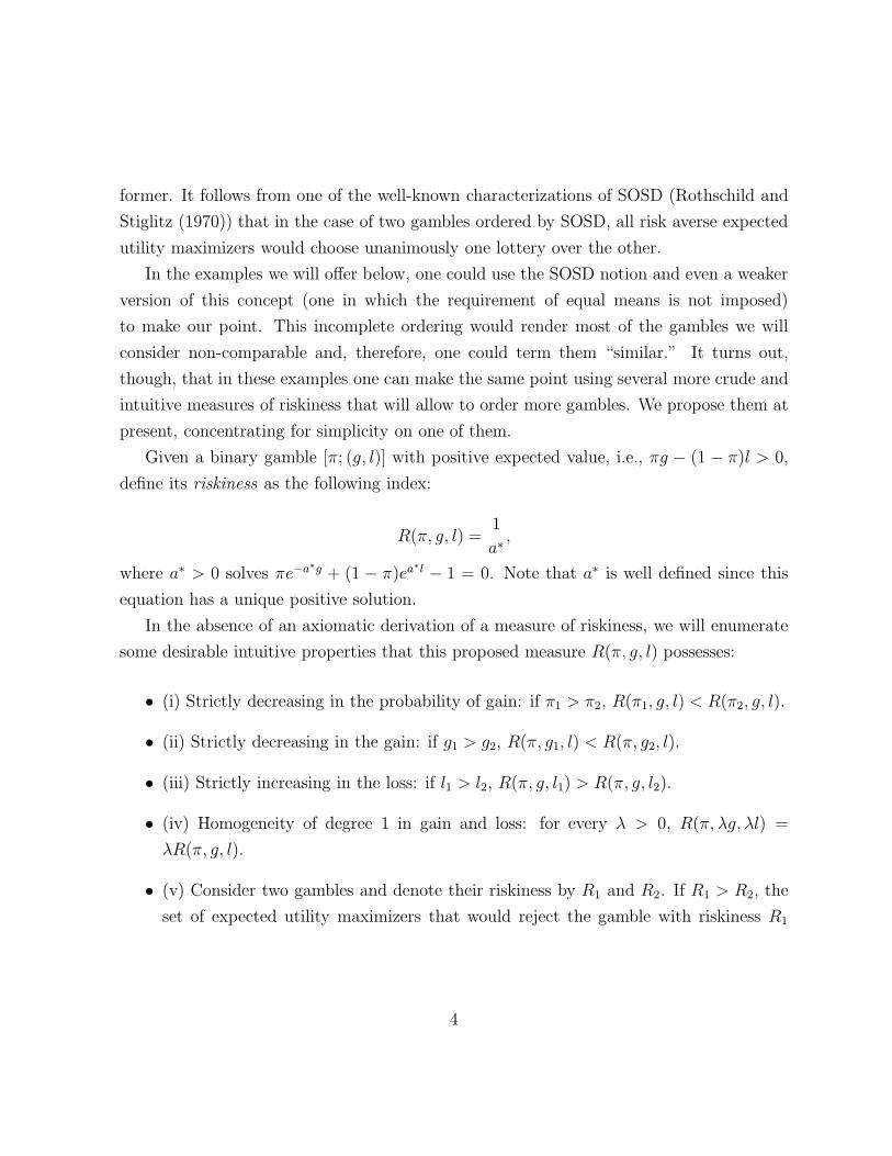
Given a binary gamble [π; (g, l)] with positive expected value, i.e., πg − (1 − π)l > 0,

define its riskiness as the following index:

R(π, g, l) =1

a∗ ,

where a∗ > 0 solves πe−a∗g + (1 − π)ea∗l − 1 = 0. Note that a∗ is well defined since this

equation has a unique positive solution.

In the absence of an axiomatic derivation of a measure of riskiness, we will enumerate

some desirable intuitive properties that this proposed measure R(π, g, l) possesses:

• (i) Strictly decreasing in the probability of gain: if π1 > π2, R(π1, g, l) < R(π2, g, l).

• (ii) Strictly decreasing in the gain: if g1 > g2, R(π, g1, l) < R(π, g2, l).

• (iii) Strictly increasing in the loss: if l1 > l2, R(π, g, l1) > R(π, g, l2).

• (iv) Homogeneity of degree 1 in gain and loss: for every λ > 0, R(π, λg, λl) =

λR(π, g, l).

• (v) Consider two gambles and denote their riskiness by R1 and R2. If R1 > R2, the

set of expected utility maximizers that would reject the gamble with riskiness R1

4

strictly contains the set of expected utility maximizers that would reject the gamble

with riskiness R2.3

Therefore, we shall say that a gamble with positive expected value is more risky than

another if it has a higher value of the index R. For our purposes, this is a simple statistic

that can be computed on all the gambles we will study. Its dimension is the one of the

random variable, telling us for example that Rabin’s [0.5; (105, 100)] gamble is 10 times

more risky than the [0.5; (10.50, 10)] gamble, a property that seems intuitive for the current

discussion. In addition, this index gives us a clean measure of riskiness that abstracts from

wealth considerations.

The R index just defined is by no means the only measure of riskiness we could use in

the examples of the next subsection which will show that many people accept gambles that

are riskier than Rabin’s. For example, one could also define riskiness on the basis of other

one-parameter families of preferences, or appeal to related notions found in the literature,

as follows:

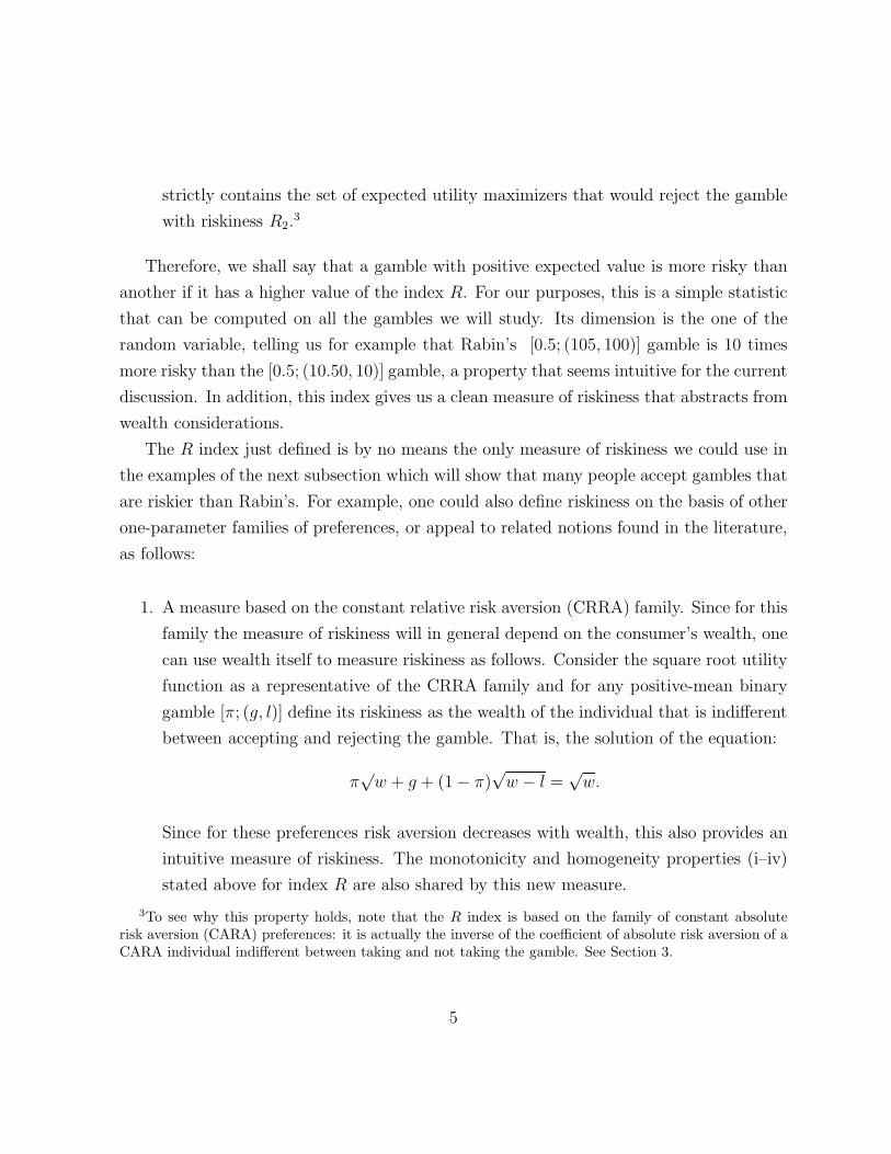
1. A measure based on the constant relative risk aversion (CRRA) family. Since for this

family the measure of riskiness will in general depend on the consumer’s wealth, one

can use wealth itself to measure riskiness as follows. Consider the square root utility

function as a representative of the CRRA family and for any positive-mean binary

gamble [π; (g, l)] define its riskiness as the wealth of the individual that is indifferent

between accepting and rejecting the gamble. That is, the solution of the equation:

π√

w + g + (1 − π)√

w − l =√

w.

Since for these preferences risk aversion decreases with wealth, this also provides an

intuitive measure of riskiness. The monotonicity and homogeneity properties (i–iv)

stated above for index R are also shared by this new measure.

3To see why this property holds, note that the R index is based on the family of constant absoluterisk aversion (CARA) preferences: it is actually the inverse of the coefficient of absolute risk aversion of aCARA individual indifferent between taking and not taking the gamble. See Section 3.

5

2. A measure based on a family of preferences that satisfy the axioms of Yaari’s (1987)

dual theory of choice under risk. Consider the family of preferences over lotteries

[π, (g, l)] that can be represented by the function −l + πα(g + l) for α > 0. It can be

shown that the bigger the α the larger the level of risk-aversion exhibited by these

preferences. For any lottery [π, (g, l)] we can find the α∗ of the individual that is

indifferent between accepting and rejecting the lottery, and define the riskiness of

the lottery as lα∗ . It can be checked that this measure also satisfies properties i–iv

mentioned above.

This family is of special interest because it is based on non-expected utility prefer-

ences.

3. The variance/mean ratio. This measure is pervasive in much of the finance literature,

especially in models of portfolio decisions.

In order to measure the riskiness of a gamble, one could choose any of these indices, the

R index or the SOSD concept. In the examples we will discuss next, similar statements

can be made using any of them.

2.2 Empirical Evidence

Out of the different ways outlined to measure riskiness of a gamble, we shall concentrate

on one of them, the R index. We proceed to calculate the values of R for different small

gambles. For us, as for Rabin (2000) and the related literature, “small gambles” simply

means that the stakes are a small fraction of consumers’ wealth.

First, we report the values of R for different Rabin gambles. Consider the gamble

[0.5; (10.50, 10)]. It has a value of R of 210. The gamble [0.5; (105, 100)] has a value of R

of 2,100.

Next we report the values of R for gambles taken from daily life experiences. They

show that individuals may well accept gambles whose riskiness, as measured by the R

index, is greater than 2,100.

1. Cicchetti and Dubin (1994) investigate the decision of whether to purchase insurance

against the risk of telephone line trouble in the home for approximately 10,000 residential

6

customers. The average price of this insurance was about g = $0.45 a month (in some

areas the price was above and in others below this amount), while the average cost of

repair in case of trouble was about $55 leading to a loss l = 55 − 0.45. Note that we

identify the gamble with not taking the insurance: hence, g represents the savings of not

paying for the insurance, and l is the net loss in the event of line trouble. The probability

of line trouble was about (1 − π) = 0.005, ranging from 0.00318 to 0.00742. A 42.9% of

users in the sample chose not to buy insurance, so these users were taking a small gamble.

The R index associated with the average consumer facing the gamble [0.995, (0.45, 54.55)]

is 59.64. However, it is not difficult to see that many households were actually taking a

gamble whose R index was far greater than 2,100. For instance, if the cost of repair is just

a few dollars above the average (in fact, if we consider the cost associated with not having

phone service for one or two days until the line is repaired, this may well be the case for

most people in the sample), say that it is $63.45, then, if (1 − π) = 0.007, the R index

of [0.993; (0.45, 63)] is 2,239. In the areas where the cost of insurance is a bit below 0.45

dollars, say 0.39 dollars and the repair cost is 55.39, the R index of [0.993; (0.39, 55)] is

2,590. These examples show that it is not difficult to find values around the average values

of π, g and l that would indicate that many individuals were taking a gamble riskier than

Rabin’s [0.5; (105, 100)].4

An observation regarding the “average gamble” is in order. Consumers were actually

facing a more risky gamble than the average one. The reason is that the typical consumer

was facing a distribution of repair costs. By replacing this distribution with its average,

one is underestimating the riskiness of the true gamble.

2. Evans and Viscusi (1991) use marketing survey data to study the implicit risk-dollar

tradeoffs that consumers make when buying certain products. They consider products

that may cause some minor health hazard such as insecticides and toilet bowl cleaners.

The cheaper insecticides and toilet bowl cleaners are associated with a risk of injury, and

the authors find that consumers identify the minor health hazard with a loss in income.

(a) In the case of insecticides, let g be the savings per bottle of a cheaper insecticide

4It can also be shown that some individuals in the sample were even taking gambles with negativeexpected value.

7

and l the monetary loss associated with the risks of injury (skin poisoning, inhalation and

child poisoning). Probabilities are π = 0.9985 and (1 − π) = 0.0015 for no-injury and

injury per bottle, respectively. Take the gamble [0.9985; (7.84, 4589)] at the average of the

data. This gamble has an R index of about 18,000. We thus conclude that the average

person in the sample accepts a gamble that is riskier than Rabin’s [0.5; (105, 100)].

It is not difficult to consider values around the average values of g, l and the probability

π using the standard deviations reported in their article so that we would cover virtually

all the individuals in the sample. We would then find even greater differences in riskiness

with respect to Rabin’s gambles.

(b) In the case of toilet bowl cleaners, let g denote savings per bottle of a cheaper

toilet bowl cleaner and l the monetary loss associated with the risks of injury (eye burns,

gassings and child poisoning). Probabilities are π = 0.9985 for no-injury and (1 − π) =

0.0015 for injury, per bottle. Take the gamble at the average of the data for g and l:

[0.9985; (2.23, 2000)]. This gamble for the “average consumer” has a negative expected

value. This consumer would be taking an unfair gamble. One can easily generate other

gambles with negative mean if one plays around with different values of π, g and l that fit

well within the sample. It is also easy to find gambles with positive mean that are riskier

than Rabin’s. For instance, the gamble [0.999; (2.23, 2000)] has an R index of about 9,200.

The next example shows that in an experimental situation using real money, subjects

may often accept riskier gambles than the type Rabin (2000) assumes they reject.

3. Henrich and McElreath (2002) report experiments with real money with university

undergraduates at UCLA choosing between $15 for sure and a 50-50 gamble of win $30 or

$0. More than 80 percent of students chose the risky option, which is effectively to take

the gamble [0.5; (15, 15)]. When asked to choose between $15 for sure and a 20-80 gamble

of win $75 or $0, i.e., the gamble [0.2; (60, 15)], over 52 percent of the students chose the

risky gamble. Thus, at least 80 and 52 percent of the students, respectively, were accepting

small gambles of zero expected value.5

5The authors are interested in studying the extent to which small-scale rural farmers in differentethnographic contexts are risk averse or risk lovers. In addition to the UCLA undergraduates, theystudy the behavior of Mapuche, Huinca, and Sangu peasants in an experimental setting using real money,broadly equivalent to one-third of a day’s wage. Most of these peasants, especially the Mapuche, were

8

We close this section by noting the only empirical evidence that Rabin and Thaler

(2001) cite in their favor. They refer to Fehr and Gotte (2002) who report that about

50% of a sample of bicycle messengers in Zurich rejected the gamble [0.5; (8, 5)]. The R

index for this gamble is 13.57. Clearly, all our previous examples exhibit much higher

values of the R index. But if the threshold is to show that individuals may accept real

gambles with values of the R index greater than just 13.57, then it is easy to find further

evidence. For instance, in Holt and Laury (2002) individuals have to choose between two

risky options involving different probabilities and stakes. In one of their many treatments

individuals were asked to choose between gain 100 with probability 0.7 and gain 80 with

probability 0.3 (option A), and gain 192.5 with probability 0.7 and gain 5 with probability

0.3 (option B). Over 40% of individuals chose option B over option A, that is effectively

take the gamble [0.7; (92.5, 75)], whose R index is 77.77.

In Table I we report the values of the different indices of riskiness discussed in the

previous subsection for the several gambles considered here. It is apparent that one reaches

similar conclusions using any of these measures.

[Table I about here]

The examples in this section critically question the empirical validity of Rabin’s as-

sumption of rejecting small gambles (assumption q) without specifying the decision maker’s

preferences. We next argue that, while q can be challenged by studying how individuals

behave and say they would behave when facing small gambles, it is unclear where one

should draw the line to be satisfied with evidence supporting or invalidating Rabin’s as-

sumption q. The reason is that in the typical sample there may be both acceptors and

rejectors of the same small gamble under consideration. We thus propose to bring to bear

empirical evidence obtained under the expected utility assumption. Much of the empirical

literature attempts to find a model of preferences, along with other constructs of the mod-

els, that be a “good fit” for all the observed behavior. As explained for example in Segal

and Spivak (1990), any expected utility agent with a differentiable utility function must

accept infinitesimal gambles of positive expected value, because locally these preferences

more risk-prone than the UCLA undergraduates.

9

amount to risk neutrality. However, as soon as the gambles are of any non-infinitesimal

size, expected utility is compatible with both accepting and rejecting small gambles. It is

then necessary to perform careful econometric analyses to find the best possible fit for the

observed behavior.

3 Risk Attitudes under Expected Utility

This section shows that Rabin’s assumption q (rejecting small gambles) under p (expected

utility) implies a specific positive lower bound on the coefficient of absolute risk aversion. It

then shows that in the case of Rabin’s gambles, this lower bound turns out to imply that the

assumed values of the relative risk aversion coefficient are much higher than the estimates

ever obtained in the empirical literature. Thus, the evidence demonstrates that the joint

hypothesis “p and q” is empirically invalid. As such, it is not at all surprising that Rabin

finds highly paradoxical rejections of large-stakes gambles, that is that “p and q” implies

unrealistic behavior. However, our reason to translate Rabin’s (2000) joint assumption into

the language of risk aversion coefficients is to apply it to his very same exercises. Indeed,

the main point of this section is to replicate them, but using in them a joint assumption “p

and q” that implies empirically plausible levels of relative risk aversion. In sharp contrast

with his result, our finding is that Expected Utility implies then no paradoxical behavior.

3.1 Rejecting Small Gambles: Testable Implication on Risk Aver-sion Coefficients

For a decision maker with wealth level w and twice continuously differentiable Bernoulli

utility function u, denote the Arrow-Pratt coefficient of absolute risk aversion by ρA(w, u) =

−u′′(w)u′(w)

, with the coefficient of relative risk aversion being defined as ρR(w, u) = w·ρA(w, u).

Note that ρA(w, u) = ρR(w, u) = 0 for a risk neutral individual, while they are positive for

a strictly concave u.

Rabin (2000) shows that if an individual is a risk averse expected utility maximizer

[assumption p] and rejects a given gamble of equally likely gain g and loss l, g > l, over

a given range of wealth levels [assumption q], then he will reject correspondingly larger

10

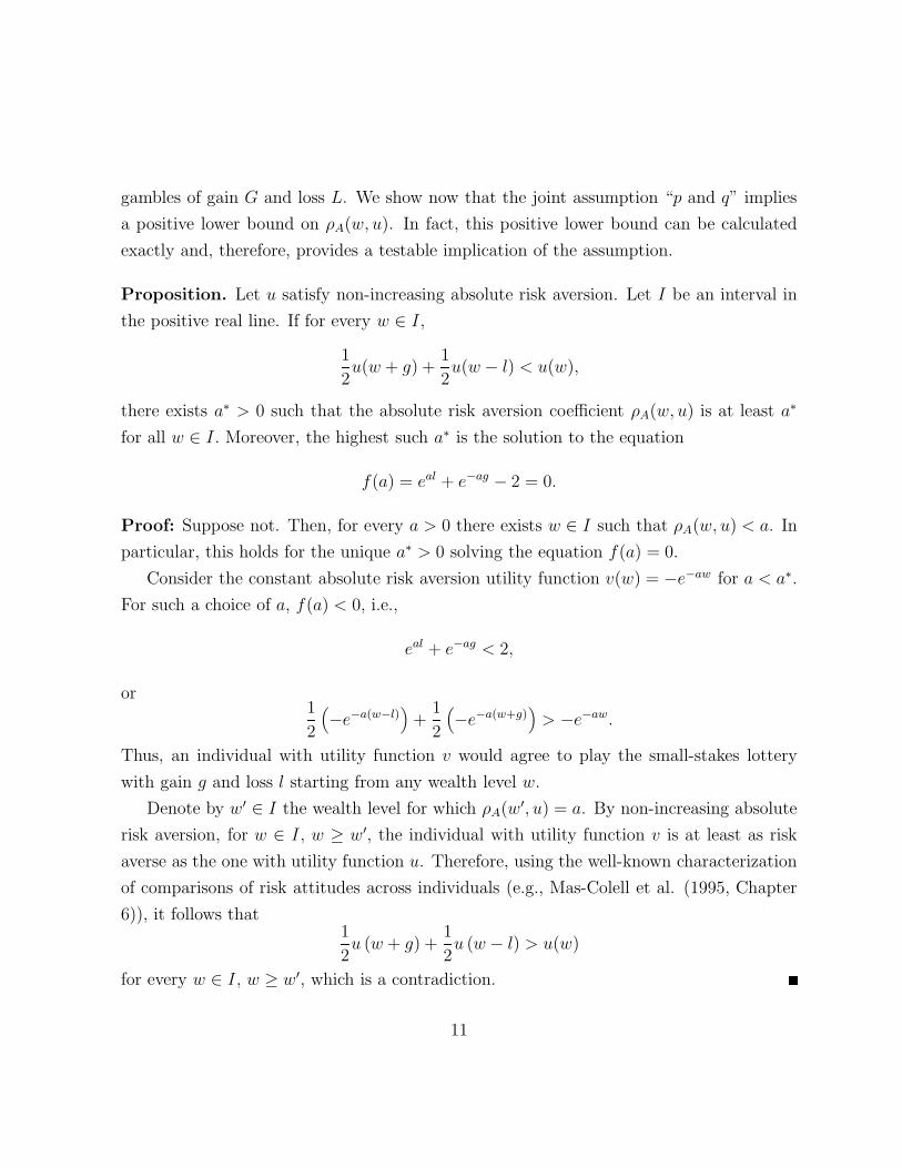
gambles of gain G and loss L. We show now that the joint assumption “p and q” implies

a positive lower bound on ρA(w, u). In fact, this positive lower bound can be calculated

exactly and, therefore, provides a testable implication of the assumption.

Proposition. Let u satisfy non-increasing absolute risk aversion. Let I be an interval in

the positive real line. If for every w ∈ I,

1

2u(w + g) +

1

2u(w − l) < u(w),

there exists a∗ > 0 such that the absolute risk aversion coefficient ρA(w, u) is at least a∗

for all w ∈ I. Moreover, the highest such a∗ is the solution to the equation

f(a) = eal + e−ag − 2 = 0.

Proof: Suppose not. Then, for every a > 0 there exists w ∈ I such that ρA(w, u) < a. In

particular, this holds for the unique a∗ > 0 solving the equation f(a) = 0.

Consider the constant absolute risk aversion utility function v(w) = −e−aw for a < a∗.

For such a choice of a, f(a) < 0, i.e.,

eal + e−ag < 2,

or1

2

(−e−a(w−l)

)+

1

2

(−e−a(w+g)

)> −e−aw.

Thus, an individual with utility function v would agree to play the small-stakes lottery

with gain g and loss l starting from any wealth level w.

Denote by w′ ∈ I the wealth level for which ρA(w′, u) = a. By non-increasing absolute

risk aversion, for w ∈ I, w ≥ w′, the individual with utility function v is at least as risk

averse as the one with utility function u. Therefore, using the well-known characterization

of comparisons of risk attitudes across individuals (e.g., Mas-Colell et al. (1995, Chapter

6)), it follows that1

2u (w + g) +

1

2u (w − l) > u(w)

for every w ∈ I, w ≥ w′, which is a contradiction.

11

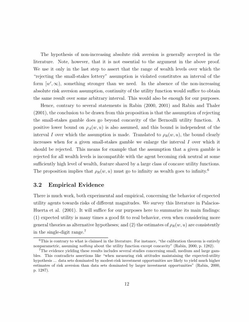
The hypothesis of non-increasing absolute risk aversion is generally accepted in the

literature. Note, however, that it is not essential to the argument in the above proof.

We use it only in the last step to assert that the range of wealth levels over which the

“rejecting the small-stakes lottery” assumption is violated constitutes an interval of the

form [w′,∞), something stronger than we need. In the absence of the non-increasing

absolute risk aversion assumption, continuity of the utility function would suffice to obtain

the same result over some arbitrary interval. This would also be enough for our purposes.

Hence, contrary to several statements in Rabin (2000, 2001) and Rabin and Thaler

(2001), the conclusion to be drawn from this proposition is that the assumption of rejecting

the small-stakes gamble does go beyond concavity of the Bernoulli utility function. A

positive lower bound on ρA(w, u) is also assumed, and this bound is independent of the

interval I over which the assumption is made. Translated to ρR(w, u), the bound clearly

increases when for a given small-stakes gamble we enlarge the interval I over which it

should be rejected. This means for example that the assumption that a given gamble is

rejected for all wealth levels is incompatible with the agent becoming risk neutral at some

sufficiently high level of wealth, feature shared by a large class of concave utility functions.

The proposition implies that ρR(w, u) must go to infinity as wealth goes to infinity.6

3.2 Empirical Evidence

There is much work, both experimental and empirical, concerning the behavior of expected

utility agents towards risks of different magnitudes. We survey this literature in Palacios-

Huerta et al. (2001). It will suffice for our purposes here to summarize its main findings:

(1) expected utility is many times a good fit to real behavior, even when considering more

general theories as alternative hypotheses; and (2) the estimates of ρR(w, u) are consistently

in the single-digit range.7

6This is contrary to what is claimed in the literature. For instance, “the calibration theorem is entirelynonparametric, assuming nothing about the utility function except concavity” (Rabin, 2000, p. 1282).

7The evidence yielding these results includes several studies concerning small, medium and large gam-bles. This contradicts assertions like “when measuring risk attitudes maintaining the expected-utilityhypothesis ... data sets dominated by modest-risk investment opportunities are likely to yield much higherestimates of risk aversion than data sets dominated by larger investment opportunities” (Rabin, 2000,p. 1287).

12

The pattern on the single-digit estimates of ρR(w, u) is remarkable. It has been obtained

in many different settings, under very different circumstances and for very different sizes of

risk. In sharp contrast with this, Rabin’s assumption that an expected utility person turns

down gambles where she loses $100 or gains $105 for any initial wealth level implies that

ρR(w, u) must go to infinity when wealth goes to infinity, while the assumption that a 50-50

lose $100 or gain $105 bets is turned down for any lifetime wealth level less than $350,000

implies a value of the same coefficient no less than 166.6 at $350,000. The strikingly large

discrepancy between the size of these coefficients and the ones observed empirically may

explain the paradoxes in Rabin (2000).8

We shall now tackle the key issue of this section: we pose the question of whether or not

rejecting Rabin’s gambles over smaller wealth intervals, those corresponding to single-digit

values of ρR(w, u), induces paradoxical behavior. We study it in the next subsection, and

remark that the answer is a priori far from obvious.

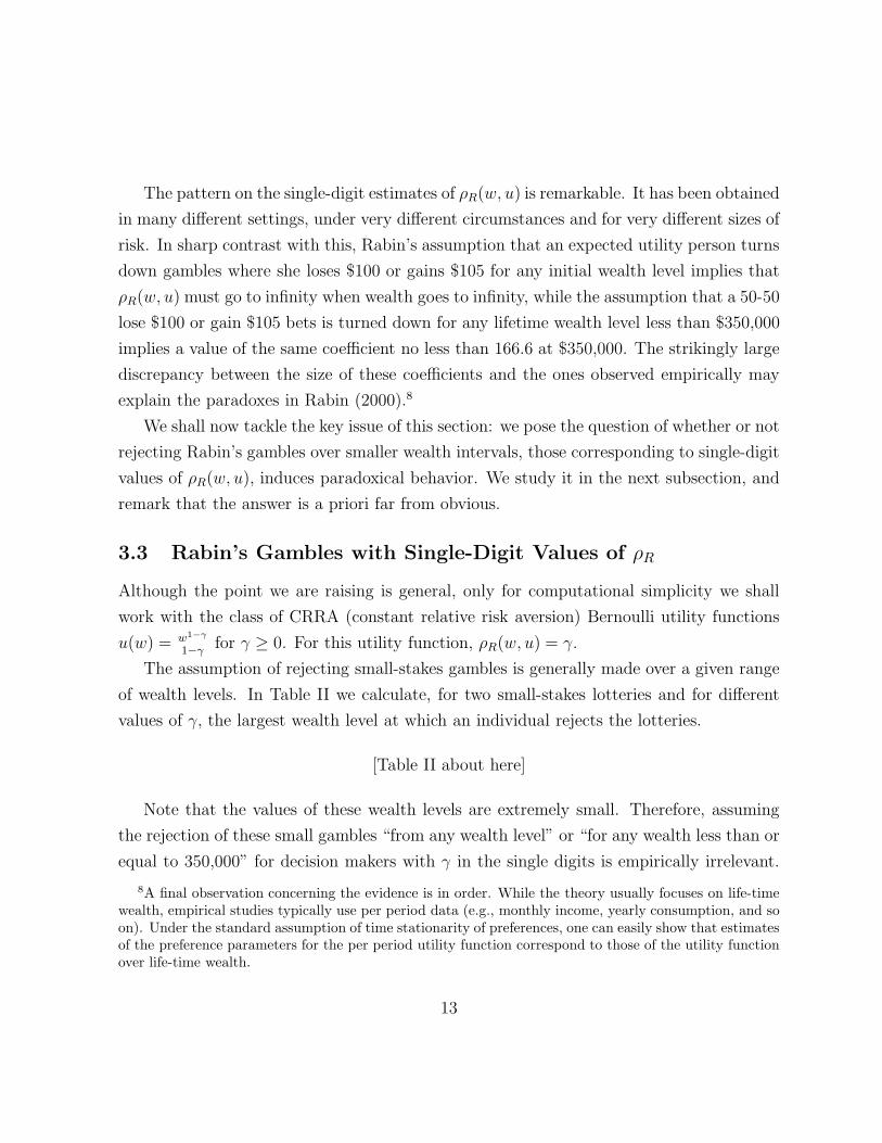
3.3 Rabin’s Gambles with Single-Digit Values of ρR

Although the point we are raising is general, only for computational simplicity we shall

work with the class of CRRA (constant relative risk aversion) Bernoulli utility functions

u(w) = w1−γ

1−γfor γ ≥ 0. For this utility function, ρR(w, u) = γ.

The assumption of rejecting small-stakes gambles is generally made over a given range

of wealth levels. In Table II we calculate, for two small-stakes lotteries and for different

values of γ, the largest wealth level at which an individual rejects the lotteries.

[Table II about here]

Note that the values of these wealth levels are extremely small. Therefore, assuming

the rejection of these small gambles “from any wealth level” or “for any wealth less than or

equal to 350,000” for decision makers with γ in the single digits is empirically irrelevant.

8A final observation concerning the evidence is in order. While the theory usually focuses on life-timewealth, empirical studies typically use per period data (e.g., monthly income, yearly consumption, and soon). Under the standard assumption of time stationarity of preferences, one can easily show that estimatesof the preference parameters for the per period utility function correspond to those of the utility functionover life-time wealth.

13

Put it differently, individuals’ behavior is not consistent with the idea that they are viewing

these choice situations in terms of life-time wealth levels.9

Continuing with the specification of CRRA utility, the next question we examine is

how high is the bound a∗ associated with the given small-stakes lottery of gain g and loss

l. On the basis of the same lotteries used in Rabin’s (2000) Tables II and III, we calculate

in Table III their corresponding values of a∗, as defined in the proposition above. The

table also shows, for wealth levels of $300,000 and $30,000, the induced values of γ.

[Table III about here]

It is first worth noting that for the wealth level of $300,000 very few values of γ are in

the single-digit range, or even in the teens. No single-digit value arises when the gamble

involves losing $100 or $1,000. Only when the rejected gamble involves losing l = $10, 000,

which would not appear to be a small-stakes gamble, such low values start to arise consis-

tently. In an attempt to generate more γ coefficients in the single-digit range, we examine

the same lotteries for a wealth level as low as $30,000. In this case, single-digit coefficients

arise for some gambles where l = $1, 000, and for all gambles where l = $10, 000, which are

hardly small-stake gambles for an individual with that wealth level. For the lowest stakes

gambles involving l = $100 a single-digit γ is only found when g = 101. We conclude

from Table III that empirically plausible, single-digit, values of γ are compatible with the

assumption only when the loss l in the gamble is a significant proportion of the individ-

ual’s wealth. In other words, the empirically plausible version of assumption q imposes

the rejection of the small gambles over a much smaller interval of wealth levels than those

used in Rabin (2000).

Next we try to replicate Rabin’s results, but imposing that γ be in the single-digit

range, which would correspond to imposing assumption q over a suitably smaller interval

of wealth levels. We wish to find out whether this still induces paradoxical behavior.

9As a referee noted, subjects may view lab choice situations and “short-term” problems in isolation,rather than in conjunction with other sources of income. Moreover, as Rubinstein (2001) notes, “nothingin the von Neumann-Morgenstern (vNM) axioms dictates use of final wealth levels ... vNM are silentabout the definition of prizes ... The definition of prizes as final wealth levels is no less crucial to Rabin’sargument than the expected utility assumption.”

14

For various lotteries in Table III that yield values of γ in the single-digit range, Table

IV replicates the exercise in Rabin (2000) and displays the best large-stakes lottery with

gain G and loss L that the decision maker would reject.

[Table IV about here]

It is apparent that these rejections are no longer paradoxical. For instance, for a

wealth of $300,000 the agent turns down gambles involving losses L ranging from 5 to

15 percent of his wealth and gains G that appear reasonable. The same can be said for

a wealth of $30,000. In this case, note that relative to wealth these values of L are ten

times greater than those in Rabin (2000). Thus, not even for these much larger gambles

paradoxical behavior is obtained. Finally, it is worth stressing that gambles with G = ∞are turned down only when potential losses L represent a significantly great proportion of

the individual’s wealth.

The reasonable behavior described in these large-stakes gambles contrasts with the

paradoxes in Rabin (2000) and in other authors in the literature, and may be viewed as a

further confirmation of the empirical soundness of single-digit values for ρR(w, u).

These results refute assertions such as “paradoxical implications are not restricted to

particular contexts or particular utility functions,” or “within the expected-utility frame-

work, for any concave utility function, even very little risk aversion over modest stakes

implies an absurd degree of risk aversion over large stakes” (Rabin (2001, p. 203)). That

is, much more than “very little risk aversion over modest stakes” is needed to generate

paradoxical behavior. Indeed, as we have shown, this is only obtained when the assump-

tion q is made over too large an interval of wealth levels, which corresponds to a region of

the parameter space that is not empirically relevant.

4 Concluding Remarks

Using a problem posed to one of his colleagues as a starting point, Samuelson (1963)

argues that, under expected utility, the rejection of a given single gamble for all wealth

levels implies the rejection of the compound lottery consisting of the single gamble being

15

repeated an arbitrary number of times. Samuelson’s exercise sheds light on the fact that

some decision makers may be misapplying the law of large numbers when accepting a

compound lottery (the colleague’s response was that he would reject the single lottery,

but accept its compound version). However, Samuelson was clearly aware of the crucial

importance of the assumption of rejecting the single lottery for all wealth levels or a large

range thereof: “I should warn against undue extrapolation of my theorem. It does not say

that one must always refuse a sequence if one refuses a single venture: if, at higher income

levels the single tosses become acceptable, and at lower levels the penalty of losses does not

become infinite, there might well be a long sequence that it is optimal” (p. 112). Indeed, it

may very well be the case that Samuelson’s colleague was not fooled by any fallacy of large

numbers. He simply violated the assumption of rejecting the given small-stakes lottery for

all wealth levels or large range thereof.

The main advantage of expected utility is its simplicity and its usefulness in the analysis

of economic problems involving uncertainty. As often argued in the literature, its predic-

tions sometimes conflict with people’s behavior. This has led economists to develop various

non-expected utility models which can often accommodate actual behavior better. The

non-expected utility research agenda is an important one, and there is no question that

we should continue to pursue it. However, expected utility should not be accused when it

is not at fault. The analysis in this paper shows how certain paradoxical examples in the

literature are many times counterfactuals.

In a more recent paper, Rabin and Thaler (2001) continue to drive home the theme

of the demise of expected utility and compare expected utility to a dead parrot from a

Monty Python show. To the extent that all their arguments are based on introspection

and on the calibrations in Rabin (2000), not on empirical evidence, the expected utility

parrot may well be saying that “the report of my death was an exaggeration.”

16

REFERENCES

Arrow, K. J. Essays in the Theory of Risk Bearing. Chicago, IL: Markham PublishingCompany, 1971.

Cicchetti, C. J. and J. A. Dubin. “A Microeconometric Analysis of Risk Aversion andthe Decision to Self-Insure.” Journal of Political Economy 102 (1994): 169-186.

Epstein, L. G. “Behavior under Risk: Recent Developments in Theory and Applications.”In J. J. Laffont (ed.) Advances in Economic Theory. VI World Congress of the EconometricSociety (vol. II), Cambridge University Press, 1992.

Evans, W. N. and W. K. Viscusi. “Estimation of State-Dependent Utility FunctionsUsing Survey Data.” Review of Economics and Statistics 73 (1991): 94-104.

Fehr, E. and L. Gotte. “Do Workers Work More if Wages Are High? Evidence froma Randomized Field Experiment,” Working Paper No. 125, Institute for Empirical EconomicResearch, University of Zurich, 2002.

Friedman, M. and L. J. Savage. “The Utility Analysis of Choices Involving Risk.” Journalof Political Economy 56 (1948): 270-304.

Hansson, B. “Risk Aversion as a Problem of Cojoint Measurement.” In Decision, Probabil-ity, and Utility, ed. by P. Gardenfors and N.-E. Sahlin. Cambridge: Cambridge University Press,1988.

Henrich, J. and R. McElreath. “Are Peasants Risk-Averse Decision Makers?” CurrentAnthropology 43 (2002): 172-181.

Holt, C. A. and S. K. Laury. “Risk Aversion and Incentive Effects.” American EconomicReview 92 (2002): 1644-1655.

Kandel, S., and R. F. Stambaugh. “Asset Returns, Investment Horizon, and Intertem-poral Preferences.” Journal of Monetary Economics 27 (1991): 39-71.

Machina, M. “Expected Utility Analysis without the Independence Axiom.” Econometrica50 (1982): 277-323.

Mas-Colell, A., M. D. Whinston and J. R. Green. Microeconomic Theory, OxfordUniversity Press, 1995.

Palacios-Huerta, I., R. Serrano and O. Volij, “Rejecting Small Gambles under Ex-pected Utility,” Working Paper 2001-05, Department of Economics, Brown University and Eco-nomics Working Paper 32, Institute for Advanced Study, http://www.sss.ias.edu/papers/econpaper32.pdf,2001.

Pratt, J. “Risk Aversion in the Small and in the Large.” Econometrica 32 (1964): 122-136.Rabin, M. “Risk Aversion and Expected-Utility: A Calibration Theorem.” Econometrica

68 (2000): 1281-1292.Rabin, M. “Diminishing Marginal Utility of Wealth Cannot Explain Risk Aversion.” In

Choices, Values, and Frames. D. Kahneman and A. Tversky, eds. Cambridge University Press,2001.

17

Rabin, M. and R. H. Thaler. “Anomalies. Risk Aversion.” Journal of Economic Per-spectives 15 (2001): 219-232.

Rothschild, M. and J. E. Stiglitz. “Increasing Risk: I. A Definition.” Journal ofEconomic Theory 2 (1970): 225-243.

Rubinstein, A. “Comments on the Risk and Time Preferences in Economics.” Mimeo(2001), Tel Aviv and Princeton University.

Samuelson, P. A. “Risk and Uncertainty: A Fallacy of Large Numbers.” Scientia 98 (1963):108-113.

Segal, U. and A. Spivak. “First Order versus Second Order Risk Aversion.” Journal ofEconomic Theory 51 (1990): 111-125.

Watt, R. “Defending Expected Utility Theory.” Journal of Economic Perspectives 16(2002): 227-229.

Yaari, M. E. “The Dual Theory of Choice under Risk.” Econometrica 55 (1987): 95-115.

18

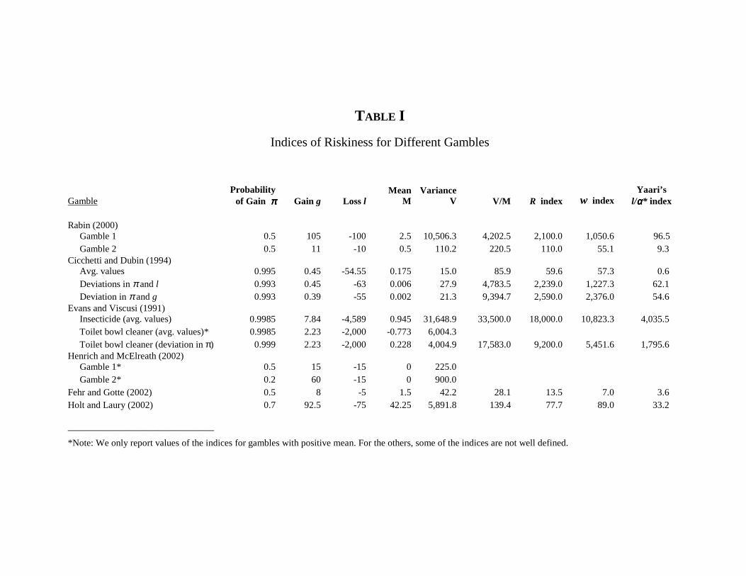
TABLE I

Indices of Riskiness for Different Gambles

Gamble Probability

of Gain ππππ Gain g Loss l Mean

M Variance

V V/M R index

w index Yaari’s

l/αααα* index Rabin (2000) Gamble 1 0.5 105 -100 2.5 10,506.3 4,202.5 2,100.0 1,050.6 96.5 Gamble 2 0.5 11 -10 0.5 110.2 220.5 110.0 55.1 9.3 Cicchetti and Dubin (1994) Avg. values 0.995 0.45 -54.55 0.175 15.0 85.9 59.6 57.3 0.6 Deviations in π and l 0.993 0.45 -63 0.006 27.9 4,783.5 2,239.0 1,227.3 62.1 Deviation in π and g 0.993 0.39 -55 0.002 21.3 9,394.7 2,590.0 2,376.0 54.6 Evans and Viscusi (1991) Insecticide (avg. values) 0.9985 7.84 -4,589 0.945 31,648.9 33,500.0 18,000.0 10,823.3 4,035.5 Toilet bowl cleaner (avg. values)* 0.9985 2.23 -2,000 -0.773 6,004.3 Toilet bowl cleaner (deviation in π) 0.999 2.23 -2,000 0.228 4,004.9 17,583.0 9,200.0 5,451.6 1,795.6 Henrich and McElreath (2002) Gamble 1* 0.5 15 -15 0 225.0 Gamble 2* 0.2 60 -15 0 900.0 Fehr and Gotte (2002) 0.5 8 -5 1.5 42.2 28.1 13.5 7.0 3.6 Holt and Laury (2002) 0.7 92.5 -75 42.25 5,891.8 139.4 77.7 89.0 33.2 _______________________________

*Note: We only report values of the indices for gambles with positive mean. For the others, some of the indices are not well defined.

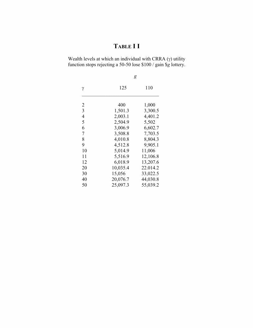
TABLE I I

Wealth levels at which an individual with CRRA (γ) utility function stops rejecting a 50-50 lose $100 / gain $g lottery.

g

γ 125 110 _______________________________ 2 400 1,000 3 1,501.3 3,300.5 4 2,003.1 4,401.2 5 2,504.9 5,502 6 3,006.9 6,602.7 7 3,508.8 7,703.5 8 4,010.8 8,804.3 9 4,512.8 9,905.1 10 5,014.9 11,006 11 5,516.9 12,106.8 12 6,018.9 13,207.6 20 10,035.4 22.014.2 30 15,056 33,022.5 40 20,076.7 44,030.8 50 25,097.3 55,039.2

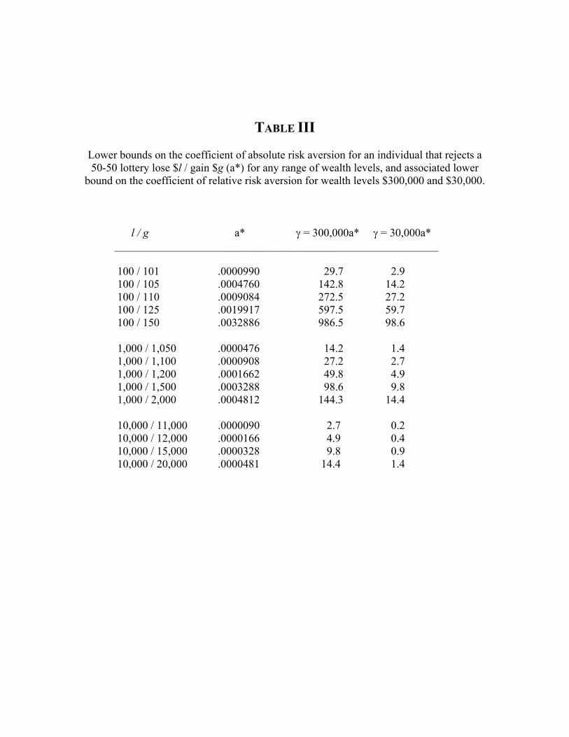
TABLE III

Lower bounds on the coefficient of absolute risk aversion for an individual that rejects a 50-50 lottery lose $l / gain $g (a*) for any range of wealth levels, and associated lower

bound on the coefficient of relative risk aversion for wealth levels $300,000 and $30,000.

l / g a* γ = 300,000a* γ = 30,000a* __________________________________________________________

100 / 101 .0000990 29.7 2.9 100 / 105 .0004760 142.8 14.2 100 / 110 .0009084 272.5 27.2 100 / 125 .0019917 597.5 59.7 100 / 150 .0032886 986.5 98.6

1,000 / 1,050 .0000476 14.2 1.4 1,000 / 1,100 .0000908 27.2 2.7 1,000 / 1,200 .0001662 49.8 4.9 1,000 / 1,500 .0003288 98.6 9.8 1,000 / 2,000 .0004812 144.3 14.4

10,000 / 11,000 .0000090 2.7 0.2 10,000 / 12,000 .0000166 4.9 0.4 10,000 / 15,000 .0000328 9.8 0.9 10,000 / 20,000 .0000481 14.4 1.4

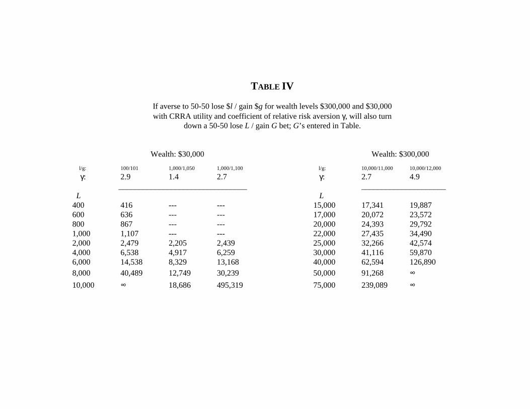
TABLE IV

If averse to 50-50 lose $l / gain $g for wealth levels $300,000 and $30,000 with CRRA utility and coefficient of relative risk aversion γ, will also turn

down a 50-50 lose L / gain G bet; G’s entered in Table.

Wealth: $30,000 Wealth: $300,000

l/g: 100/101 1,000/1,050 1,000/1,100 l/g: 10,000/11,000 10,000/12,000 γ: 2.9 1.4 2.7 γ: 2.7 4.9

________________________________ _____________________ L L

400 416 --- --- 15,000 17,341 19,887 600 636 --- --- 17,000 20,072 23,572 800 867 --- --- 20,000 24,393 29,792 1,000 1,107 --- --- 22,000 27,435 34,490 2,000 2,479 2,205 2,439 25,000 32,266 42,574 4,000 6,538 4,917 6,259 30,000 41,116 59,870 6,000 14,538 8,329 13,168 40,000 62,594 126,890 8,000 40,489 12,749 30,239 50,000 91,268 ∞ 10,000 ∞ 18,686 495,319 75,000 239,089 ∞