Reintegrating ex-rebels into civilian life:Evidence from a quasi-experiment in Burundi!

Michael Gilligan1, Eric Mvukiyehe2, and Cyrus Samii†21Department of Politics, New York University

2Department of Political Science, Columbia University

May 5, 2010

Abstract

Abstract will go here...

1 Introduction

Disarmament, demobilization and reintegration (DDR) programs are central to international inter-

ventions to assist countries coming out of civil war. These programs, often provided for in peace

agreements1, are typically carried out alongside economic reconstruction, infrastructure rehabil-

itation, institutional reform, refugee repatriation and democratization. All of these interventions

aim to address the root causes of conflict and reduce the likelihood of another war (Boutros-Ghali!This research is part of the Wartime and Post-conflict Experiences in Burundi survey, sponsored by the Folke

Bernadotte Academy, Sweden, and United States Institute of Peace. We thank Iteka - Ligue Burundaise des Droitsde l’Homme for being our partners. We are grateful to Dingamadji Solness and Marcelo Fabre from the WorldBank/Multi-Country Demobilization and Reintegration Program and members of the executive secretariat of Burundi’sCommission Nationale de Demobilisation, Reintegration et Reinsertion. We thank participants at the February 2009conference on Evolution de la pauvrete et du bien-etre au Burundi in Bujumbura and especially Phillip Verwimp fororganizing it. This research comes under IRB-approved protocols at Columbia University (no. AAAB8249) and NewYork University (no. HS-5279). This work is solely the authors’ responsibility, and in no way represents the positionof the above-named organizations.

†The authors are listed by alphabetical order. Correspondence may be sent to Cyrus Samii via email atcds81@columbia.edu.

1Not all DDR take place in the framework of peace agreements. In several cases, like Rwanda and Ethiopia, DDRwas undertaken after the military defeat of one side. In Colombia, DDR was launched while the civil war was ongoing.Some DDR programs take place as part of army reform processes, such as those that followed World War II and theCold War (Kingma and Pauwels 2000). This paper focuses on internationally-sponsored DDR in post-conflict settings.

1

1992; Cousens et al 2001; Paris 2004; Doyle and Sambanis 2006). DDR programs are usually im-

plemented under the direction of international actors, especially the United Nations (UN) and the

World Bank. DDR programs encompass a set of activities designed to lay the foundation of stable

and self-sustaining peace. These activities entail the discharge of a large number of combatants

who must be disarmed and reintegrated into civilian life (Walter 2001; Fortna 2008).

The disarmament and demobilization of former combatants—the first two components of DDR—

take place before the reintegration phase in order to create security conditions and trust necessary

for implementing peace agreements (Spear 2002). The security resulting from effective disar-

mament and demobilization is also a prerequisite for the roll-out of recovery and development

activities (Kumar 1997; Rubin et al. 2003; Feil 2004). A goal following disarmament and demo-

bilization is for demobilized combatants to find a livelihood and submit to laws and norms that

govern civilian society. Based on a presumption that the former combatants cannot or will not

achieve this automatically, reintegration programs supplement disarmament and demobilization

processes. Reintegration programs typically encompass a wide range of activities that include (i)

short-term measures such as the provision of cash assistance or in-kind material benefits to address

the immediate needs of former combatants and their dependents upon leaving armed groups; and

(ii) longer-term measures such as vocational training, skill development and counseling, which aim

to reintegrate former combatants into the social and economic structures of society (Colletta et al.

1996; Bryden et al.2005; Muggah 2009). The literature that informs the design of current rein-

tegration programs tends to presume that ex-rebels form a class that, on average, exhibits serious

human and social capital deficiencies. If these deficiencies are not attended to, the presumption

is that they would significantly limit ex-combatants’ ability to establish themselves economically,

making them susceptible to recruitment into armed groups or criminality. Sometimes program de-

signers may appreciate that ex-combatants are no more vulnerable than their civilian counterparts,

but that they need extra incentives to be steered from the temptations of banditry and extortion—

activities that their combatant experience has trained them to do. Finally, in some contexts (e.g.

those in which where rebels have won control of the government), reintegration assistance is jus-

tified as necessary for honoring the sacrifices of combatants who were not integrated into a new

2

armed forces.

Reintegration is a critical component of DDR both because it links “the more immediate re-

quirements of disarmament and demobilization to the long-term imperatives of social and eco-

nomic welfare” (Bryden et al.2005) and because it is the set of activities that facilitate effective

conversion from combatant to civilian life.2 Effective conversion to civilian life is achieved not

only when former combatants are able to establish peaceful and sustainable livelihoods (“economic

reintegration”), but also when they longer see force and violence as a legitimate means to pur-

sue their objectives (“political reintegration”; World Bank, 2002; United Nations, 2000; Pouligny

2004).3 The ability to establish good working relations with one’s community or family (“so-

cial reintegration”) is often taken to be an important moderator of an ex-combatant’s economic and

political reintegration prospects. The typical causal model is social reintegration " economic rein-

tegration " political reintegration. Reintegration programs typically emphasize economic reinte-

gration. They also include reconciliation interventions that attempt to facilitate social reintegration,

but these are usually secondary. Political reintegration is not usually directly targeted, but political

reintegration is presumed to follow from the boost that a program provides to social and economic

reintegration. Spear (2006) argues that among post-conflict interventions, reintegration is the most

directly “linked to establishing a lasting peace” (emphasis in the original)—a conclusion echoed

by Cavallo’s (2008) argument that effective reintegration of former combatants is a “sine qua non”

for the consolidation of peace.

Despite the importance of reintegration programs, there have been few attempts to evaluate

their effectiveness (Humphreys and Weinstein 2007; Muggah 2009). Some macro-level studies

exist, particularly studies evaluating the reintegration programming of major international insti-2In practice reintegration has been the most neglected component of DDR—at least in terms of funding. Some an-

alysts argue that the fact that reintegration is not strictly a military activity can explain this relative neglect. As Specker(2008) notes “The limited time horizon and the preponderance of security concerns of the international community,however, frequently resulted in resources being used primarily for the DD-phases, leaving inadequate funding for theR-phase.”

3Rackley (2007) argues that donors have the mistaken idea that “as soon as you get guns out of their hands, theyare suddenly innocuous human beings again, but that is not the case at all” (cited in Hanson 2007). Indeed, whiledisarmament and demobilization processes are key mechanisms to “it reduce the capacity of the former combatantsto renew armed conflict” (Russett and O’Neil 2001), they are by themselves not sufficient to transform old soldiersinto civilians. To complete the conversion process, as Rackley discusses, former combatants must be provided with aneconomic alternative to living by the gun.

3

tutions like United Nations agencies and the World Bank, and they typically focus on program

performance and outputs.4 There are also several descriptive studies that focus on the practical

challenges that fraught the implementation of reintegration programs,5 and a growing critical liter-

ature that questions the assumptions that underpin these programs.6 However, focusing as they do

on macro factors like reintegration program design and conflict settlement terms, these studies tell

us very little about the effectiveness of reintegration programs in helping individual ex-combatants

reintegrate into civilian life.

A handful of recent studies has relied on ex-post surveys and other micro-level data to try to

identify effects of reintegration programs. Humphreys and Weinstein (2007) investigate the effects

of a UN-sponsored DDR program in Sierra Leone. They found reintegration programming to have

no measurable effect on improving reintegration prospects, while contextual factors such as wealth

and education (ironically) as well as wartime traumas seemed to hinder economic reintegration.

Pugel (2006) and Muggah and Bennett (2009) conducted a similar studies in Liberia and Ethiopia,

respectively. They both find some evidence (albeit differentiated) of program impacts [SUCH

AS???? TO BE INSERTED...].

These quantitative studies have had only a modest effect on thinking about reintegration due

mostly to the weak possibilities that they offer for identifying causal effects. The weakness is by

no fault of the authors, but rather from the nature of the programs. The material benefits offered

by such programs makes the incentive to participate very strong, meaning that those who do not

participate are likely to differ in important ways from those who do. In Sierra Leone, for example,

rates of participation in the UN-sponsored reintegration program were around 90 percent, in which

case the non-participants used to construct the pseudo “control group” (as in Humphreys and We-

instein, 2007) are likely to be a highly self-selected group, even after controlling for observable

confounders. Using “completion of the program” only adds additional layers of endogeneity. In the

absence of some random shock to program access, identifying impacts of reintegration programs

is a task that requires more assumptions than most people would be comfortable to make.4See, for example, Colletta et al (1996) and the studies contributed to the Government of Sweden’s Stockholm

Initiative on Disarmament, Demobilization, and Reintegration (2006).5See, for example, Kingma (1997); UNDP, 2000; Alden (2002); Paes (2005); Baare (2006) and Specker (2008).6See, for example, Pouligny (2004); Muggah (2005) and Jennings (2008).

4

In this paper we exploit such a shock, which occurred during the reintegration program in

Burundi and thus allows us to measure reintegration program effects with minimal taint from

selection bias. A peace process in 2003-4 ended a decade of civil war in Burundi. Under the

terms of the agreement, a National Commission for Disarmament, Demobilization and Reintegra-

tion program—CNDDR by its French acronym—was established to run a reintegration program

with the support of the United Nations Operation in Burundi (UNOB) and the World Bank’s Multi-

country Disarmament and Reintegration Programs (MDRP). A small number of non-governmental

organizations (NGOs) were contracted to deliver reintegration training and business start-up pack-

ages. An idiosyncratic bureaucratic failure caused reintegration programming to be unexpectedly

withheld for a large segment of would-be beneficiaries who were on line to receive a training and

economic reintegration package in 2006-2007. The failure was due to planning errors and com-

plications in the personal relationship between CNDRR officials and one of the newly contracted

NGOs, Africare. For the segment of beneficiaries registered in the region covered by Africare, the

reintegration package was withheld for about a year, although it was available to peers who were

assigned to the other agencies. During this time, would-be beneficiaries in the Africare region

were forced to live their lives without a reintegration package. In the middle of this period, we

fielded a large-scale a survey in Burundi. By making well-structured comparisons between those

whose could not receive program benefits with those who could, we have a quasi-experiment on

the effects of reintegration programming. Specifically, we can study whether the program had the

desired impact on economic reintegration, and whether such impacts themselves have translated

into political reintegration.

The paper begins by discussing the outcomes of interest and hypotheses pertaining to reinte-

gration programming. We then discuss the more specific context of rebel reintegration in Burundi

in the aftermath of the civil war from 1993-2004 and the nature of the reintegration assistance

that the program provided. We then describe the methods that we use to identify effects of the

program—or more correctly, effects of the non-availability of the program—and then present our

estimates of effects on economic and political reintegration.

5

2 Defining reintegration outcomes

This paper investigates the effectiveness of reintegration programming in Burundi. The United Na-

tions defines reintegration as “the process which allows ex-combatants and their families to adapt,

economically and socially, to productive civilian life” (United Nations, 2000). Reintegration has

social, economic and political dimensions. Social reintegration refers to an ex-combatant’s re-

lations with family and members of his or her community. Economic reintegration refers to an

ex-combatant’s ability to find a productive and sustained livelihood in the post-war context. Politi-

cal reintegration refers to an ex-combatant’s commitment to the laws and norms of civilian society,

and especially, commitment to peaceful and democratic political expression (IDDRS 2.10). In this

paper, we study economic and political reintegration. Economic reintegration is the direct target

of most reintegration assistance (Spear 2006), including in Burundi. Because economic reintegra-

tion is presumed to facilitate political reintegration, we also measure effects on the latter, and we

attempt to tease out whether economic effects may have contributed to political reintegration.

The primary objective of economic reintegration programs is to help ex-combatants gain sus-

tained livelihoods and enhance the economic welfare (World Bank, 2002; 2004). This objective is

based on the premise that a propensity to participate in violence is largely determined by the non-

violent livelihood options available to an individual. This objective also draws from the research

program on the political economy of conflict, which emphasizes the role of economic opportuni-

ties in reducing the risk of conflict (Collier and Hoffler 2004). In its 2003 report entitled Breaking

the Conflict Trap, the largest sponsor of reintegration programs, the World Bank, claimed that “a

structured DDR process, which demobilizes combatants in stages and emphasizes their ability to

reintegrate into society, may reduce the risk of ex-combatants turning to violent crime or joining

rebel groups in order to survive” (emphasis added). There are some reasons to believe that ex-

combatants may face fewer economic opportunities and therefore be prone to engage in violence.

First, ex-combatants may lack human and social capital endowments necessary to establish them-

selves economically.7 These deficiencies may emanate from characteristics that set apart those7For broad-brush reviews on possible sources of vulnerability among ex-combatants, see Annan and Patel (2009)

and Tajima (2009).

6

who decided to participate in fighting , or they may be consequences of soldiering itself. Thus,

ex-combatants may also face acute shortages of material capital. Time spent away soldiering may

have caused an ex-combatant to have had his or her land taken over by someone else; or, for those

with no land endowments to start with, time spent soldiering may have made it difficult for the

person to acquire land. These deficiencies may put ex-combatants at an economic advantage and

make them more likely to engage in banditry to support themselves. This suggestion is consistent

with findings from Collier’s (1994) research on demobilization and reintegration of former sol-

diers in Uganda. He finds that lack access to land significantly increased the likelihood of these

former soldiers to commit crime, at least in the short-term. From this perspective, economic rein-

tegration programs can reduce the risk of ex-combatants’ involvement in criminality by addressing

their human and social deficiencies and helping them become more competitive for employment

opportunities.8

Economic reintegration may also affect opportunity costs associated with ongoing violent con-

flict. According to this logic, ex-combatants are rational actors who weigh costs and benefits of

war and peace economies and may not return to civilian life unless the latter provide them with

greater economic incentives. There are two sides to this argument. The first is that some combat-

ants may have joined armed groups for economic reasons and thus economic reintegration can be

seen as addressing these motivations. As Spear (2006) notes “an emphasis on [economic reinte-

gration] recognizes that some of the motives for fighting were economic and that if the economic

dimensions of the problem are not addressed, any settlement of the conflict may be short-lived.”

Second, the absence of law and order in conflict situations may provide combatants with oppor-

tunities to enrich themselves through illicit means, including robbery, racketeering and smuggling

(Reno 1997). Ending the war is tantamount to giving up these economic opportunities—a prospect

that may not be very appealing to many of them unless reintegration packages are attractive. There8Some analysts suggest that the problem of postwar reintegration is not so much that ex-combatants have human

and social capital deficiencies, but rather that the local economies they reintegrate into have very few economic oppor-tunities available for them. For instance, speaking of the economic reintegration challenges faced by ex-combatants inMozambique, McMullin (2004) notes “post-conflict states with impoverished economies offer little to reintegrate into.Mozambique, where only a tenth of the population had formal employment, was not exception, giving rise to quip:‘the government told us “now you are all equally poor. You have been reintegrated back into basic poverty” (emphasisin original).

7

is anecdotal evidence suggesting that at least some combatants make these sorts of calculations.

During the DDR process in Liberia, a member of one of the Liberian United for Reconciliation

and Democracy (LURD)—the main rebel group during the second civil war—was reported to say

that “I still have my 81-mm mortar, but I just come to see whether the UN was giving fighters who

disarm something good, If they don’t give good money, I will not give the rocket” (Agence France

Press, 8 December 2003; cited in Spear 2006). This is an example of spoiler behavior that Stedman

(1997) argued can derail the peace process if not dealt with appropriately. More worrisome, how-

ever, is that ex-combatants like the one described above can become vulnerable to manipulation

by elites who may want to start another war (Russett and O’Neal 2001). From this viewpoint, by

providing a range of economic benefits and incentives, reintegration programs make civilian life

more attractive and this can reduce the risk of conflict.

These logics constitute channels through which reintegration failure might destabilize the deli-

cate peace in the aftermaths of civil war. As Alden (2002) remarks, “the spectre of former military

personnel in criminal networks in the Balkans and Russia, the outbreak of violence inspired by

real and self-proclaimed war veterans in Zimbabwe, and the participation of former security force

members from Eastern Europe and South Africa in mercenaries in war-torn Angola and the Congo

serve to underscore the destabilizing role played by former combatants who remain outside of the

economy and society as a whole.” Given that reintegration programs are seen as a key mechanism

to prevent renewed armed conflict and their centrality in international peacebuilding interventions,

there is an urgent need to ascertain their effectiveness.

There are two interrelated hypotheses associated with interventions that intend to boost eco-

nomic reintegration. The first hypothesis is that reintegration programs can substantially improve

the economic welfare of ex-combatants. The second is that improved economic welfare can sub-

stantially increase an ex-combatants’ respect for the peace agreement and the rule of law. This

paper investigates these hypotheses with quasi-experimental evidence in Burundi. We look at

whether reintegration programming affected monetary income, occupational choice, and subjec-

tive assessments of economic-well-being. We then look at whether reintegration programs have an

effect of increasing ex-combatants’ satisfaction with the peace agreement and commitment to the

8

rule of law.

3 The Burundi context

We focus on the reintegration of adult (18+) male former rebel combatants in Burundi. Members

of the national army were also demobilized and offered reintegration assistance, but we do not

study them. The reintegration experience of former army members is likely to be quite different

than for former rebels. Being an army soldier is a legal, well defined career. Demobilization and

reintegration support is well institutionalized: certain members of the national army had access to

a system of pension-type benefits that were separate to those put in place by the internationally

assisted reintegration program. The legality and institutionalized nature of an army career implies

that there are fewer questions about demobilized army soldiers’ “place in society.” For these rea-

sons, we do not think it is warranted to lump the two subgroups together. We choose to focus on

reintegration of former rebels, which we believe to be of utmost interest to reintegration program

designers. We focus on men only because we think women’s experiences are likely to be distinct,

but our sample of women is too small to study them adequately. Finally, we focus on former rebels

who were aged 18 years or older as of fieldwork in 2007. Some of them were recruited before

adulthood,9 but they were all adults at the time of their demobilization, which could have been

up to 3 years prior to fieldwork. Ex-combatants under 18 were treated by a different (UNICEF-

managed) reintegration program than adults, in which case outcomes associated with them would

not necessarily be comparable to those above the age cut-off.10

The DDR program in Burundi was initiated following a 2003-4 ceasefire that drew into the

peace process the largest rebel group in the country, the National Council for the Defense of

Democracy-Forces for the Defense of Democracy, or CNDD-FDD by its French acronym. At

the time of our fieldwork in 2007, one rather small rebel faction—the Agathon Rwasa faction of9The youngest ex-rebel in our sample is 19, and the years of recruitment for our respondents was between 1993

and 2003.10Such a strict age cut-off creates an opportunity for a possibly well-identified examination of the benefits of pro-

gramming for those just under 18 relative to those just over 18. This is something that could be pursued in furtherwork. Those under 18 received considerably more support relative to their counterparts over 18 in mending relationswith family and community members. Thus, there is a ripe opportunity for studying the impacts on social reintegrationand the downstream benefits of social reintegration on economic and political reintegration.

9

the National Forces for Liberation, or FNL by their French acronym—remained outside the peace

process. The war had begun in 1993 in aftermath of a tumultuous attempt at democratization.

Elections in 1993 had resulted in the triumph of a party that represented the aspirations of a long-

oppressed Hutu majority. Under still-mysterious circumstances, members of the southern- and

Tutsi-dominated army led a failed coup attempt in October 1993; the coup attempt nonetheless

involved the assassination of the recently-elected president. The event triggered massive violence

throughout the country. The ensuing ferment gave way to outright civil war. The war had a dev-

astating impact on the tiny, landlocked central-African country. Fighting touched most of the

country. It resulted in deaths estimated at approximately 300,000 out of a total population of 6-8

million. Burundi’s pre-war socio-economic development levels were already among the world’s

lowest, although for its income level, the country did have relatively well-developed infrastructure

and institutions. The war severely stalled development for over a decade, resulting for example in

an estimated 20% decline in real GDP over 1993-2002 (World Bank 2004, p. 6).

The outcome of the war and ensuing political developments are important features of the en-

vironment into which ex-rebels were reintegrating. The war resulted in a peace accord between

the government and the CNDD-FDD that called for elections. Significantly, the 2005 elections

resulted in the CNDD-FDD winning an outright majority of national assembly seats (59% of 118

seats) and communal councilor posts (55% of 3,225 posts). This gave the party the strength nec-

essary to elect its political head, Pierre Nkurunziza, to be president. As such, the outcome of the

war brought about a near revolution in the institutionalized political context relative to before the

war. As of 2005, the former rebels were elected to lead. Contrast this to outcomes in the other

countries where reintegration has been studied: in Sierra Leone, the party of former rebels, the

Revolutionary United Front Party, managed barely 2% of votes, failing to win a single seat in the

2002 elections that punctuated the end of the war. In Uganda, the Lord’s Resistance Army is still an

illegal organization, never having had its popular legitimacy tested. Though the number of cases is

too small to test the claim rigorously, there is good reason to believe that conditions causing rebel

parties to fair well electorally are associated with reintegration prospects of demobilized rebels.

These considerations should be taken into account when trying to generalize the findings from this

10

paper.

The 2000 Arusha Accords called for DDR, and these Accords set the parameters of the 2003

Pretoria agreement, which brought the CNDD-FDD into the peace process and set the stage for the

2005 elections. A February 2004 World Bank report set specific DDR targets; a November 2004

Joint Operations Plan (JOP), which was approved by a committee that included all key national

and international agencies, made these targets official (World Bank 2004; Republic of Burundi

2004; Boshoff and Vrey 2006, p. 15). The MDRP and national implementing agencies designed

a program that was intended to demobilize and reintegrate enough combatants to achieve a new

army (Forces de Defense Nationale) of 25,000 and police force of 20,000.11 The World Bank’s

estimates for the sizes of the various forces is shown in Table 1. Both members of the national

army and the rebel groups would be demobilized. DDR would occur in two phases, with the first

phase (2004-5) involving 9,000 former rebels and 5,000 former army. Those not demobilized in

the first phase would then join an interim integrated national army and police. Over the ensuing

years, some 41,000 additional combatants from the newly integrated security forces were to be

demobilized as part of a broader army and police reform program.

The DDR program in Burundi was part of the broader Multi-Country Demobilization and

Reintegration Program (MDRP)12, which was intended to embody a comprehensive strategy to

“enhance prospects for stabilization and recovery in the region.” The program documentation for

the MDRP’s programs reflected a strong presumption that demobilized combatants would likely

suffer human and social capital deficits that would have to be remedied, otherwise “disaffected

ex-combatants can pose a threat to stability.” The MDRP characterized economic reintegration

as the establishment of “sustainable livelihoods.” Assistance was to do no more than would be

“necessary to help them attain the general standard of living of the communities into which they11The original project proposal set a demobilization target of 55,000 combatants. However, this target appears to

have been an error: the size of the various forces prior to demobilization was estimated to be about 80,000. The targetarmy plus police force size was 45,000. If no new recruitment was to take place, somewhere around 35,000 would needto be demobilized. Recruitment into the new armed forces was to take place, but no where near the 20,000 that wouldmake the 55,000 number realistic. The actual number demobilized as of June 2007 (the time of fieldwork) was about23,000; to date, the total is about 28,000, about half the 55,000 target proposed in 2004 This error is acknowledged inWorld Bank (2009).

12Participating countries included Angola, Burundi, Central African Republic, Democratic Republic of Congo,Rwanda, Republic of Congo, and Uganda.

11

reintegrate” (19). Social reintegration, in the form “reconciliation” between ex-combatants and

civilians in their communities, was taken to be an important pre-condition for achieving a sus-

tainable livelihood. The program took an “individual-oriented” approach—one that emphasized

providing means to individual ex-combatants, as opposed to trying to do much at the level of

communities; this orientation was apparently due to an implicit agreement that would have other

agencies—namely UNDP—taking responsibility for community reconstruction.

The reintegration program included a few components. The CNDRR directly administered a

reinsertion subsistence allowance of XXX Burundian Francs (FBu, with 500 FBu equivalent to 1

2007 dollar in PPP terms) provided in X tranches over XX months. Documentation from the pro-

gram shows that at the time of our fieldwork in 2007, receipt of these tranches was nearly universal

among ex-combatants (XX%).13 Also, through offices set up in nearly all provinces and through

“focal points” appointed in nearly all communes, ex-combatants had access to various forms of

counseling, including psychological counseling. These too were universally available. Thus, rein-

sertion allowances and counseling are not sources of variation in our study. The major benefit

offered by the program was the so-called “socio-economic reintegration package.” The package

provided a menu of opportunities from which ex-combatants could choose. They could choose to

be admitted into secondary school or university, to take up a one-year or shorter vocational-training

program, or to take up a package to help begin “income-generating activities.” The latter would

involve working with one of the reintegration program’s implementing partners to devise a busi-

ness plan, receiving basic training on running a business, and being provided with in-kind start-up

materials (money was not given). Program documentation shows that the “income-generating ac-

tivities” option was by far the most popular, with XX% taking up this option, in comparison to X%

taking up vocational training and X% pursuing their education [I NEED TO GET THE SPECIFICS

FROM THE MDRP QUARTERLY REPORTS.]

The CNDRR and MDRP delegated the delivery of the socio-economic reintegration package

benefits to NGO partners. Early in the program, when the number of beneficiaries processed13Interestingly, the allowance was administered through transfers to special bank accounts for ex-combatants, giving

many ex-combatants their first exposure to bureaucracy and the formal banking sector. Interviews in the field revealedthat some ex-combatants applied what they learned through this by offering for-profit services to help other peopledeal with banks and government offices.

12

and ready to receive benefits was rather small, a large and rather disorganized collection of local

NGOs was contracted on an ad hoc basis to deliver benefits. In 2006, anticipating a surge in the

number of ex-combatants who would be coming online to receive benefits, the MDRP decided

to tighten up the system and contracted three large NGOs to deal with the coming wave of ex-

combatants. These included PADCO and Twitezimbere, two Burundian NGOs, and Africare, an

international NGO. The work was divided evenly among the three NGOs. PADCO was assigned

to cover ex-combatants registered as residents in the south-west provinces, Twitezimbere was to

cover ex-combatants registered as residents in the northern provinces, and Africare was to cover

ex-combatants registered as residents in the center provinces. The assignments to the three NGOs

were made by the end of the summer in 2006, and programming was to begin as soon as possible.

The selection of Africare as one of the three partners was due to pressure by MDRP donors to

have at least one of the implementing partners be an international NGO; the pressure was due to

certain budget limitations, it seems. This was the case despite the program administrators’ and

the CNDRR’s concerns about the readiness of Africare to implement the program.14 Indeed, it

came to be a major problem: while PADCO and Twitezimbere were able to begin quite quickly,

Africare’s presence on the ground was barely established by late 2006.15 This was followed by a

contracting dispute between CNDRR and Africare that caused further delays. As a result, desig-

nated beneficiaries in the Africare area were denied access to the reintegration package until late

2007. This disruption in program access corresponded to the timing of our fieldwork: PADCO

and Twitezimbere had begun reintegration programming by late 2006, whereas the problems with

Africare’s commencement of delivery would not be resolved until August 2007. Our fieldwork was

conducted in June/July 2007. Thus, the respondents in our sample from the PADCO/Twitezimbere

areas had access to reintegration programming, but those from the Africare areas did not, or at

best, were only just beginning to have access. So long as any other differences between sample

respondents from “center” areas and other areas can be controlled for, this bureaucratic breakdown

provides us with a source of near-exogenous variation in program access. Such is the cornerstone14Interview with Marcelo Fabre, MDRP, February 2009.15Geenen (2007) notes that Africare had no presence on the ground in the area of her fieldwork, Ruyigi, in

November-December 2006, and that they expressed concerns themselves about whether they could implement theprogram.

13

of our strategy for identifying the effects of the reintegration program.

4 Identification

Two majors concern in the study of assistance programs such that is one are self-selection by

beneficiaries into the program and targeted selection of beneficiaries by the program managers.

Such selection is typically based on would-be beneficiaries’ and program managers’ predictions

about how much beneficiaries will gain by participating. Much of the information that forms such

judgments is unobservable by the analyst. In the Burundi reintegration program, the disruption in

program access was due neither to self-selection among would-be beneficiaries nor targeting by

program managers. The arbitrariness of the disruption considerably reduces the scope for con-

founding due to unobserved factors.

However, this shock to program access is imperfect as a source of quasi-random assignment at

the individual level for two reasons. First, there may have been incidental imbalances in the at-

tributes of ex-combatants in the Africare versus non-Africare regions prior to the disruption to ac-

cess. Second, the disruption in program access occurred after some ex-combatants in the Africare

region had already received their reintegration package. Unfortunately, our data do not allow us

to identify these individuals, although information from the program itself provides the true rate at

which this occurred. Third, region-level differences could confound our estimate of the disruption

effect. The rest of the section explains our strategy for identifying causal effects in the face of these

possible sources of bias.

4.1 Incidental imbalance

Because the shock to program access occurred at the region level (rather than the individual level),

incidental imbalances in the attributes of ex-combatants in the Africare and non-Africare regions

threaten the validity of causal inferences drawn from comparing the two groups. In the analy-

sis below, we study such possibilities by conducting balance checks on a rather large set of pre-

disruption covariates. We find that balance is actually quite good over this large set of covariates,

lending more credibility to the idea that the disruption in program access has the character of an

14

experiment. If such balance can be found on such a large set of observable covariates, we have

more reason to believe the unobserved factors are also in balance.

As a further step, we used a genetic matching algorithm (Sekhon, n.d.) to match Africare and

non-Africare ex-combatants on this set of covariates. Given the rather modest sample size (less

then 400 ex-rebel observations), matching achieves remarkably good balance on this large set of

covariates. Of course, we cannot control for region-wide differences that distinguish the Africare

region from the non-Africare region, as they would coincide perfectly with our shock to program

access. An identifying assumption that we make is that once the incidental individual-level differ-

ences have been accounted for in our sample, there are no remaining region-wide differences. We

examine this assumption below.

In our empirical analysis, we present (1) simple unadjusted differences between Africare and

non-Africare regions, (2) differences adjusted via regression on our covariate list, (3) unadjusted

matched differences, and (4) regression adjusted matched differences. We take (4) to be the least

biased estimate, and thus designate that as the primary estimate of the causal effect. If estimates

(1)-(3) tend to be close to (4), then we may infer that the covariate conditioning contributes little to

bias reduction, although it may make our estimates considerably less precise. In those cases, esti-

mates (1)-(3) allow us to assess the amount of precision that we are sacrificing, perhaps needlessly.

4.2 Exposure heterogeneity

The disruption in program access in the Africare region occurred after some reintegration program-

ming had already begun. Table 3 provides the relevant figures, obtained from the reintegration

program itself. We see that as of the time of our fieldwork in July 2007, the program disruption

affected 53% of designated ex-combatant beneficiaries in the Africare region. If we were to simply

measure differences between Africare and non-Africare ex-combatants, we would obtain an esti-

mate of the disruption effect that is biased toward zero. Such bias is attributable to the exposure

heterogeneity among Africare-region ex-combatants. To correct for this source of bias, we use a

strategy that weights our effect estimate by the inverse of the difference in disruption rates across

15

the Africare and non-Africare regions. To see how this works, consider the following model,

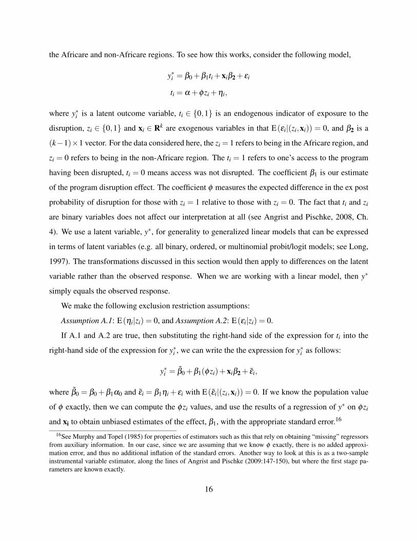
y!i = !0 +!1ti +xi!2 + "i

ti = # +$zi +%i,

where y!i is a latent outcome variable, ti # {0,1} is an endogenous indicator of exposure to the

disruption, zi # {0,1} and xi # Rk are exogenous variables in that E("i|(zi,xi)) = 0, and !2 is a

(k$1)%1 vector. For the data considered here, the zi = 1 refers to being in the Africare region, and

zi = 0 refers to being in the non-Africare region. The ti = 1 refers to one’s access to the program

having been disrupted, ti = 0 means access was not disrupted. The coefficient !1 is our estimate

of the program disruption effect. The coefficient $ measures the expected difference in the ex post

probability of disruption for those with zi = 1 relative to those with zi = 0. The fact that ti and zi

are binary variables does not affect our interpretation at all (see Angrist and Pischke, 2008, Ch.

4). We use a latent variable, y!, for generality to generalized linear models that can be expressed

in terms of latent variables (e.g. all binary, ordered, or multinomial probit/logit models; see Long,

1997). The transformations discussed in this section would then apply to differences on the latent

variable rather than the observed response. When we are working with a linear model, then y!

simply equals the observed response.

We make the following exclusion restriction assumptions:

Assumption A.1: E(%i|zi) = 0, and Assumption A.2: E("i|zi) = 0.

If A.1 and A.2 are true, then substituting the right-hand side of the expression for ti into the

right-hand side of the expression for y!i , we can write the the expression for y!i as follows:

y!i = !0 +!1($zi)+xi!2 + "i,

where !0 = !0 +!1#0 and "i = !1%i + "i with E("i|(zi,xi)) = 0. If we know the population value

of $ exactly, then we can compute the $zi values, and use the results of a regression of y! on $zi

and xi to obtain unbiased estimates of the effect, !1, with the appropriate standard error.16

16See Murphy and Topel (1985) for properties of estimators such as this that rely on obtaining “missing” regressorsfrom auxiliary information. In our case, since we are assuming that we know $ exactly, there is no added approxi-mation error, and thus no additional inflation of the standard errors. Another way to look at this is as a two-sampleinstrumental variable estimator, along the lines of Angrist and Pischke (2009:147-150), but where the first stage pa-rameters are known exactly.

16

Documentation from the program (MDRP) itself allow us to obtain a value for the true rates

of disruption in the Africare and non-Africare regions. We assume that these rates are equivalent

to the ex post expected probability of disruption conditional on whether one was located in the

Africare region or not. Our discussion with a key program official suggests that this is a reasonable

interpretation, as pre-disruption access seemed to be quite random.17 If one is wary about this, one

may take a conservative position, and assume any estimates based on this interpretation form an

upper bound; a lower bound is available by not correcting for $ at all, so informative bounds can

be constructed.

Table 3 shows the rates of disruption for the population of demobilized combatants registered

to receive benefits in the Africare and non-Africare regions. Based on this information, we take

.53$ 0 = .53 as the value of $ . The MDRP documentation also provides information on the rate

at which beneficiaries who were due to received benefits after the NGO transition actually took up

the program by the time of fieldwork in July 2007. These rates reflect the disruption in the Africare

region: at the time of fieldwork, about 66% of these post-transition beneficiaries in non-Africare

regions had already begun their engagement with the program, while only 16% had begun to do

so in the Africare region. We stress that we do not want to incorporate this information into the

construction of $ . The rate of program take-up in the non-Africare region reflects, to a large extent,

self-selection; those who had not taken up the program by then should nonetheless be considered

as having had uninterrupted access. Individuals in the non-Africare region should have factored

the availability of the reintegration program into their decision-making, and so the effect of access

to the program should be evident even among those who have chosen not to take it up. The very

small number of beneficiaries having begun engagement with the program in Africare regions after

the disruption had only recently done so at the time of fieldwork. Considering them to have been

subject to the disruption has, at worst, an effect of biasing our effect estimate toward zero. Thus, to

be clear, we are measuring the effects of disrupted access to a functioning reintegration program.

By disregarding these rates of program take-up, we actually take a more conservative approach, in

that we do not attempt to make the program look more effective by netting out any dilution due to

non-engagement by certain beneficiaries despite their having had access.17Interview with Marcelo Fabre, MDRP executive offices, February 23, 2009.

17

The above results are based on a homogenous effects model. If we loosen that assumption

to allow for variable coefficients, then we could interpret our estimate of !1 as the effect of the

program only on those whose access to the program would depend on zi (see Angrist and Pischke,

2009, Theorem 4.4.1). It seems to us that the estimate under the homogenous effects assumption is

probably higher than the true average effect of the program. This is because people who obtained

access to the program in the Africare region are likely to have been more organized generally about

their personal affairs; therefore, we suspect for them, the program’s benefits would be less. For

these reasons, we believe that the scaled estimates are likely to be an upper bound on the true

average effect. Reduced form estimates—that, is estimates from regressions using the unadjusted

zi rather than $zi—are a lower bound. We report both below.

4.3 Region level differences

To be inserted: a section that compares contextual variables in the Africare versus the non-Africare

region (excluding Buja) to assess any threats to validity that may come from differences in the

economic context. We cannot control for these factors because they will be perfectly correlated

with our indicator of program disruption. However, we can use this assessment to determine

whether any differences will likely tilt the analysis toward or away from the null.

5 Data

The ex-combatant data are drawn from the multi-purpose Wartime and Post-Conflict Experiences in

Burundi survey.18 The survey includes data from interviews with civilians, as well as ex-rebels and

ex-army, both demobilized and those integrated into the new security forces. This paper works with

only the demobilized ex-rebel data. The data were obtained through a multistage random sample

from lists of demobilized ex-rebels registered to receive reintegration benefits through Burundi’s

national DDR program (the CNDRR). The first stage involved randomly selecting half of Burundi’s

129 communes—Burundi’s second-tier administrative unit. We then set a target number of ex-

combatant interviews to complete in each commune, with targets proportional to the number of18Details on the survey are available at www.columbia.edu/&cds81/burundisurvey/

18

ex-combatants registered with the DDR program in the commune. Targets ranged from 2 to 33.

Then, we obtained from the national DDR office the complete lists of ex-combatants registered as

residents of each of the selected communes. We then drew a simple random sample (with a random

number generator in Stata) of the desired number of interviews from each of these commune lists;

we also created a randomly selected reserve list to draw from in the case of non-response. Selected

participants were contacted and brought to the respective Provincial Bureau by DDR program staff

for interview on a scheduled date by our enumeration team. The rate at which our first choice was

interviewed was very high—XX% (CHECK)—and so we assume no need for further adjustment

to account for non-response.19 This was likely due to a few factors: (1) respondents probably

took the interview to be a requirement of the DDR program given that they were contacted by the

DDR program staff themselves; (2) we accommodated respondents’ schedules by setting dates for

interviews well in advance; (3) the fieldwork was conducted during the idle interim period between

planting and harvesting seasons, and so there was little risk of non-response due to people having to

attend to agricultural demands; and (4) while participation was voluntary, a “transport allowance”

of about 2 US dollars was provided to each respondent after they completed the interview, thus

making it worthwhile for respondents to sit through the entire interview. With the observations

limited to former rebel males registered to receive reintegration assistance outside Bujumbura, the

dataset includes 110 ex-rebels registered in the Africare region and 261 outside the Africare region.

As is common in large scale surveys such as this, the data exhibit occasional missingness

on items. Such missingness is due to “don’t know” responses, enumerator error, or data-entry

error. In the subset of data that we used, only once did the item missingness rate reach 10%

for any given variable—such was the case for the measure of the death rate in an ex-combatant’s

fighting unit; otherwise the rates of item missingness were usually 0, but occasionally around 1-2%.

Listwise deletion would nonetheless have implied discarding 23% of excombatant observations. To

avoid the inefficiencies and biases associated with listwise deletion, we used multiple imputation

to fill missing values.20 Multiple imputation was conducted using the “mice” package for the19Keep in mind that the covariate adjustment that we perform below will reduce any biases associated with those

factors. With such a low non-response rate, it is reasonable to believe that any residual bias is negligible.20In additional to the loss in statistical power, listwise deletion can bias results by either discarding cases based on

the value of the dependent variable or distorting the relationship between the sample and population in ways that bias

19

R statistical computing environment (van Buuren and Groothuis-Oudshoorn, 2010). “Predictive

mean matching” imputation was used for all numeric, binary, and ordered categorical variables;

multinomial logit regression imputation was used for non-ordered categorical variables. Predictive

mean matching (also known as “nearest neighbor hot deck”) is attractive because, when the item-

level data exhibit only low levels of missingness, it is robust to a wide range of misspecifications

of the imputation model (Little and Rubin, 2002:69). Uncertainty in predictive mean matching

arises in the fit of the predictive mean model. With the multinomial logit, uncertainty arises from

the fit of the model and the fundamental uncertainty inherent in the outcome being modeled as

a random draw from a multinomial distribution. To account for these imputation uncertainties,

multiple imputed datasets should be generated (hence “multiple” imputation). The analysis should

then be run on each of the datasets, and averaged using the appropriate averaging forumlas. This

was the approach that we took, working with five imputed datasets.21

6 Inference

For primary estimation on each of the imputation-completed datasets, we use sandwich estimates

of coefficient variances that account for clustering at the commune-level. For the quantile regres-

sion estimates, we use standard errors from inverted rank-test confidence intervals asymptotically

robust to non-iid sampling (Koenker and Hallock, 2000).22 To combine the estimates from each

of the imputation-completed datasets, we used standard formulas based on the properties of mixed

normal distributions (known as “Rubin’s rules,” Rubin, 1987). If a coefficient estimate from dataset

j is called Q j, then the point estimate is simply, Q = 1m !m

j=1 Q j, the average over the m imputation-

approximations (e.g. linear or quadratic) of unknown functional forms. This is explained in Samii (2010). If multipleimputation is done in a reasonable manner, it will be considerably less biased and will generate appropriate uncertaintyestimates. See King et al (2001) for some general discussion of multiple imputation methods, and Rubin (1987) andLittle and Rubin (2002) for deeper treatments. Approximation bias is best understood through the lens of non-randomsampling. See, e.g., Korn and Graubard (1999:159-185).

21As Rubin (1987:114) explains, rather few imputations are typically needed to achieve reliable estimates.22Bootstrapped confidence intervals are inappropriate on the matched sample (Abadie and Imbens, 2008), and to

ensure comparability of results across the estimates from matched and unmatched data, we used only analyticallyderived standard errors and asymptotic confidence intervals.

20

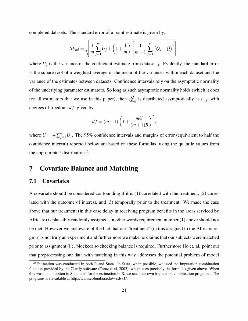
completed datasets. The standard error of a point estimate is given by,

SEmi =

!""# 1m

m

!j=1

Uj +

$1+

1m

%&1

m$1

m

!j=1

'Q j $ Q

(2),

where Uj is the variance of the coefficient estimate from dataset j. Evidently, the standard error

is the square root of a weighted average of the mean of the variances within each dataset and the

variance of the estimates between datasets. Confidence intervals rely on the asymptotic normality

of the underlying parameter estimators. So long as such asymptotic normality holds (which it does

for all estimators that we use in this paper), then QSEmi

is distributed asymptotically as t[d f ] with

degrees of freedom, d f , given by,

d f = (m$1)$

1+mU

(m+1)B

%2,

where U = 1m !m

j=1Uj. The 95% confidence intervals and margins of error (equivalent to half the

confidence interval) reported below are based on these formulas, using the quantile values from

the appropriate t distribution.23

7 Covariate Balance and Matching

7.1 Covariates

A covariate should be considered confounding if it is (1) correlated with the treatment, (2) corre-

lated with the outcome of interest, and (3) temporally prior to the treatment. We made the case

above that our treatment (in this case delay in receiving program benefits in the areas serviced by

Africare) is plausibly randomly assigned. In other words requirement number (1) above should not

be met. However we are aware of the fact that our “treatment” (in this assigned to the Africare re-

gion) is not truly an experiment and furthermore we make no claims that our subjects were matched

prior to assignment (i.e. blocked) so checking balance is required. Furthermore Ho et. al. point out

that preprocessing our data with matching in this way addresses the potential problem of model23Estimation was conducted in both R and Stata. In Stata, when possible, we used the imputation combination

function provided by the Clarify software (Tomz et al, 2003), which uses precisely the formulas given above. Whenthis was not an option in Stata, and for the estimation in R, we used our own imputation combination programs. Theprograms are available at http://www.columbia.edu/&cds81/.

21

dependence. Our concern was that those ex-combatants in the Africare areas might be substantially

different according to important covariates than their fellows in the other areas of the country that

received the treatment earlier. Therefore we have to be concerned about making inferences from

extreme counterfactuals (King and Zeng). Since we do not know the true functional form of the

relationship between our covariates and our outcome of interest (post-war economic well being

we cannot assume that we know the relationship between a given independent variable over the

whole range of a given the independent variable. By fitting a particular function (say linear) for to

the relationship between independent and dependent variables we are implicitly assuming that the

relationship between a given independent variable was the same for very hi levels of that variable

and very low levels of that variable. Pre-processing the data with matching overcome this problem

by making comparisons between treated and control cases that are very close to each other in terms

of the values of their covariates. This substantially reduces the implications of our functional form

assumptions because the difference in predicted values from various functional forms will be quite

similar where covariates are quite similar (Ho et. al, 2007, King and Zeng)

In what follows we list the variables on which we matched and our reasons for including them

in our list of covariates. In all cases the data used for the matching were taken from the Burundi

Peacebuilding Survey, implemented by the authors.

Age We hypothesize that younger ex-combatants will be less well endowed with pre-existing

skills and social networks that are necessary for successful economic reintegration. Previous

studies (?) have shown that child soldiers in particular are deprived of the crucial period of

their lives when important human and social capital skills are developed. Thus or expectation

is that younger ex-combatants may experience less economic reintegration than older ex-

combatants.

Hutu Since the war had a strong Hutu versus Tutsi ethnic component and since the predominantly

Hutu CNDD won the war we would expect Hutu ex-combatants to fare better after the war

ceteris paribus than Tutsis

Father’s education We use an indicator variable for whether the respondent’s father completed

22

primary school. We take this to be an indicator of the respondent’s family’s socio-economic

status, which is likely to correlate strongly with the respondent’s economic prospects.

Father in Agriculture Prewar An ex-combatant with a father in agriculture before the war was

probably relatively poor compared to those ex-combatants whose parents had more lucra-

tive jobs in an urban area. Thus we include this covariate as another control for the ex-

combatants’ pre-war socioeconomic status.

Prewar Education Ex-combatants with more education should, we expect, have an easier time

reintegrating into the economy after the war. For this variable we converted number of years

in education into a dichotomous variable equal to one if the ex-combatant

Prewar Wealth Because ex-combatants with greater wealth before the war should, we presume,

have higher incomes after the war we include a scale that captures the ex-combatant’s stock

of assets before the war. We created the scale based on survey respondents’ responses to

three questions: did their beds have sheets, did they own a radio, and did they own any cat-

tle. The bed-sheets and radio measures were devised after focus groups, in which these assets

were deemed markers of a household having moved beyond basic subsistence in their con-

sumption. Ownership of cows a distinctive indicator of wealth. We fit a two-parameter logis-

tic graded response model on these responses, using the “ltm” package in R (Rizopoulous,

2006). We then generated the factor scores from this model using the imputation method

described in Rizopoulos and Moustaki (2008).24 We fit the model on a pooled dataset that

included the ex-rebels as well as civilian survey respondents hailing from the same regions

as the ex-rebels. We assume that the factor loadings are common across the two groups;

including the civilians greatly improves the precision of the fit.

Prewar Relative Economic Deprivation This variable is the respondent’s own assessment of whether24We also asked respondents about whether they owned land but did not include it in the scale because there was

too little variation in the variable (about 95% of respondents indicated that they possessed land prior to the war). Ourchoice of these three indicators was based on the results of a Mokken analysis of all the indicators. That analysisshowed that these indicators loaded monotonically and contributed a moderately strong, single dimension signal (allH scores were at or above about .4; see van der Ark, 2007). We used ANOVA tests to determine whether a one, two,or even higher order logistic model fit the data best, and found that the two parameter model was optimal.

23

or not he was poorer than his neighbors. It helps to capture features of pre-war economic

status that we may not be picking up in our objective measures.

Father Alive and Socializes Most with Family, Prewar Families are the primary support net-

works for most Burundians and male adults are primary providers within these support net-

works. If an individual’s father was no longer living, then we presume that the individual’s

family support network was less robust. Individuals who tended to spend time away from

their families may not have strong ties to a support network on which they can rely after

returning from the war. Both of these factors would put the individual at a disadvantage

economically.

Prewar Urban Resident Urban residents are generally wealthier than people who live in the

countryside in Burundi. Furthermore more economic opportunities and social networks and

sources of human capital exist in urban environments than in the countryside. Therefore we

control for prewar urban residence to proxy for these characteristics of urban life.

Postwar Urban Resident Similar to argument made above urban residents have more economic

opportunities than those in the countryside so we must control for this factor which is pos-

sibly confounding to the ex-combatants economic well being. There is no concern with

post-treatment bias by including this covariate because ex-combatnts chose their locale of

residence before they entered the reintegration program.

Unit Death Rate We are concerned that ex-combatants who experienced the most mortal combat

would be more psychologically traumatized and therefore might find it more difficult to

return to normal economic activity.

Year in Faction We hypothesize that ex-combatants who were in combat longer would find it

more difficult to reintegrate into society.

Community Violence Like Unit Death Rate our concern with level of community violence is that

ex-combatants who were exposed to more violent trauma, in this case because their com-

munity was heavily affected by violence, may have a harder time reintegrating and finding

24

gainful employment.

Family Death Rate Our concern was, again, that more exposure to violence would make eco-

nomic reintegration more difficult. With this covariate we capture exposure to violence in

terms of the percentage of family members who were killed in the war. Furthermore postwar

economic opportunities are often supplied by social networks like the family. Ex-combatants

with a large percentage of family members killed would, we speculate, have fewer contacts

with which to pursue employment.

Unit had Written Rules We hypothesize that ex-combatants who were subject to more discipline

during the war should find it easier to reintegrate into civilian life. We measure the degree of

discipline of the ex-combatants life during the war with a dichotomous variable equal to one

if the ex-combatant’s unit had formal written rules of conduct and zero otherwise.

Non-CNDD Faction Member While several rebellious factions fought in the war the CNDD

came out the clear winner of the conflict. As such CNDD members had more economic

opportunities after the war than did members of other factions like the FNL. As such we

expect CNDD members to have a more successful economic reintegration experience than

non-CNDD members.

Demobilization Date Ex-combatants who demobilized earlier had a longer period to reintegrate

than did those who demobilized later so we expect ex-combatants who demobilized later to

have less success in economic reintegration.

Propensity Score In order to insure overall balance of our covariates we also matched on the

propensity score developed from all of the above mentioned variables.

7.2 Balance

Balance statistics are presented in Tables 4 through 6. Not surprisingly, given the argument we

made above about the quasi-experimental nature of the Africare treatment, many of the covari-

ates are well balanced even without matching. This was the case for age, Hutu, father’s education,

25

prewar education, prewar relative dependence, Father Alive, unit had written rules and demobiliza-

tion date. This raises the question of whether these variables are truly confounding. Despite that

concern we matched on them to insure that they remained in balance even after matching on the

covariates that were not naturally in balance. The fact that so many covariates were in balance even

without matching is evidence for our argument about the quasi-experimental nature of the Africare

treatment, which in turn should give us confidence that if there are unobserved differences between

the Africare and non-Africare regions we have some hope of achieving balance on them.

The fact that several variables were balanced before matching also has implication for how we

interpret the balance statistics later. Ho and King recommend looking at improvement in balance

rather than the standard p-scores on t- and KS tests. Their rationale is that many observations are

dropped as a result of matching procedures and so p-scores can improve simply by virtue of the

standard errors increasing as the sample size gets smaller. Imai et. al (2008) recommend, wisely

we think, that the researcher must also make sure that balance is actually improving–means are

getting closer together and observation are getting closer to the 45 degree line in the QQ plots.

We agree with their argument but hasten to point out that it is not cause for concern that some

covariates’ balance actually worsens as we attempt to achieve balance on other (previously unbal-

anced) covariates. These covariates were in balance before matching and continue to meet standard

criteria for balance after matching.

In contrast to the covariates described above there were several variables that were not bal-

anced between the Africare and non-Africare areas. These included our scale of prewar socioeco-

nomic status, pre- and post-war urban residence, unit death rates, the ex-combatant’s number of

years in his faction, level of community violence, non-CNDD faction member and the propensity

score. Ex-combatants in the Africare areas scored significantly higher on our prewar socioeco-

nomic scale than did ex-combatants in the other areas suggesting that they had significantly higher

levels of wealth ex ante than did other ex-combatants in the DDR program. Ex-combatants ser-

viced by Africare were significantly less likely to be urban residents both prior to the war and

after. Africare-serviced ex-combatants were exposed to significantly less violence than were ex-

combatants serviced by the other NGOs. Unit death rates and especially level of community vio-

26

lence were considerably lower for the former set of ex-combatants than the latter. 25

As we mentioned above, because of these substantial differences if we simply compared the

economic performance of Africare ex-combatants to ex-combatants serviced by other NGOs we

would be open to the charge of making inference from extreme counterfactuals. Since we do not

know the functional form of the relationship between these variables and economic reintegration

we may be guilty of attributing any differences between the treated and control groups to the treat-

ment when in fact it is due to one or more of the covariates behaving differently than our assumed

functional relationship. For example suppose we assume that the relationship between exposure to

violence is linear and that after controlling for the assumed linear relationship between exposure

to violence and economic reintegration we find that Africare areas enjoyed significantly less eco-

nomic reintegration than non-Africare regions. One explanation of the findings is that the delay

in receiving programming in the Africare regions caused ex-combatants to reintegrate less fully

than did those ex-combatants in other areas–strong evidence for efficacy of the DDR program.

Another explanation however is that the relationship between exposure to violence and the success

of economic reintegration is not linear but in fact exposure to violence had a marginally decreasing

affect. In that case we would be attributing the better performance on the non-Africare areas to the

fact that the program started earlier when in fact it was simply that the higher levels of exposure

to violence in the non-Africare areas did not have as deleterious effect on reintegration prospects

as our linear assumption predicted. We can avoid this problem by comparing ex-combatants in

the Africare areas that have similar levels of exposure to violence (and urban residence and so on)

to the ex-combatants in the non-Africare areas. When we do that our functional form assump-

tions have much less of an impact on our inferences because we are comparing cases in the same

“neighborhood” of the data.

The statistics in Table 4 through 6 show that we achieved excellent balance. The t-tests on

difference of means indicate that the distribution of our treated and control cases have statistically

indistinguishable means. This is true for all variables in all five samples. Indeed the lowest p-

value in the tables is 0.307. The Kolmogorov-Smirnov (KS) tests also show that we have achieved25In contrast family death rates were not all that different between the Africare-serviced ex-combatants and the rest

of the ex-combatants.

27

excellent balance for six of the nine variables where that test was appropriate. For these six vari-

ables over the five samples the lowest p-score is 0.166 and most were considerable higher. The

cases where balance was not so good even after matching include number of years in the faction,

community violence and the propensity score. As mentioned above even in these cases we have

excellent balance as measured by the t-test on the difference of means tests. Furthermore in most

cases there is convergence in the variances of the treated and control groups, so we have good

balance at least on the first two moments of the treated and control distributions. Furthermore the

percentage improvement in the QQ plots, which is presented in the last column of Table 4 through

6 shows that in most case the balance on these three variables improved considerably as a result of

our matching.

8 Effects on economic reintegration

We now present results on the effects of the program disruption on three measures of economic

reintegration: (1) income and, as a consequence of income, poverty incidence; (2) livelihood,

specifically whether the respondent obtained any livelihood, an agricultural livelihood, a livelihood

in the non-agricultural, non-skilled sector, or a livelihood in the non-agricultural skilled sector; and

(3) the respondent’s own assessment of his economic well-being. All estimates are displayed in

tables and figures that are placed in the appendix. A reference guide for the various estimates is

given in Table 7. As indicated above, our primary estimates are labeled “iv.a” (lower bound, with

respect to the exposure heterogeneity adjustment) and “iv.b” (upper bound).

8.1 Income and poverty incidence

We use a linear regression to examine effects on mean “log-monthly income + 1”; that is, the

natural logarithm of monthly personal income (in Burundian Francs, or FBu) reported by the re-

sponded, with 1 added. These results are presented in Table 8. We used the natural logarithm as a

variance stabilizing transformation and to reduce sensitivity to outliers; we added 1 to handle the

few cases of zero reported income. To check for sensitivity associated with adding 1, we also fit a

Tobit regression on log of income with zero-income observations treated as censored; the results

28

were identical. Inspection of the distribution of log monthly income variable over the covariates

showed that the transformation was effective in removing heteroskedasticity, although the overall

variance of the logged variable was still quite high. This is evident in the results. While our pri-

mary estimate of the difference in means (coefficients b.iva and b.ivb) is very large, the difference

has a p-value (two-sided) of .16.

Given the noisiness of the outcome variable, even after the log transformation, we also fit a

quantile regression to study effects at difference income deciles. The quantile regression allows us

to study whether the program caused non-constant shifts in the income distribution, perhaps reduc-

ing the incidence of very low or very high income, even if the mean was not significantly affected.

Our estimates are shown in Table 9. We see very large and statistically significant differences for

lower deciles, and smaller (although still statistically significant) differences at upper deciles. The

estimates at the end points are very noisy because of sparse data below and above the 10th and

90th percentiles, respectively. The estimates show that the effect of the program was concentrated

among those who would otherwise fare very badly. to put it another way, the program introduced

a floor on one’s potential income, with these floor effects less strongly felt for those who would

otherwise earn a lot.

Figure 1 illustrates these results more clearly. In the left panel, we display income distributions

(FBu/month, on the log scale) from the five imputed datasets for the Africare respondents and for

their matched controls. We see that the Africare distribution is substantially heavier at no income

(labeled as “(None)”) and at lower income values (e.g., below 10,000 FBu/month), although the

Africare respondents also include a handful of high earners. The right panel displays the quantile

regression estimates in substantive terms. A model-adjusted fit of the actual cumulative income

distribution for Africare-region respondents is plotted with the black line and black dots. Then,

the figure plots the lower bound (white dots) and upper bound (gray dots) estimates of what the

Africare respondents’ cumulative income distribution would have been had there been no program

disruption. The horizontal bars at each dot show the 95% confidence interval for these counter-

factual predictions (refer to the table caption for more details). The figure demonstrates clearly

just how large are the differences at the lower end of the income distribution. The gray area of the

29

plot shows the region of the income distribution that is below the $1.25/day (at purchasing power

parity) poverty line. Poverty incidence among the Africare respondents is shown to be about 60%

(the point where the black line crosses from the gray into the white region). The counterfactual

distributions show that this would be an estiamted 20 percentage points (lower bound estimate) to

40 percentage points lower were there no disruption. We see that this difference is not sensitive to

the precise location of the poverty line, as we estimate large and statistically significant differences

in the income distributions for a wide range of income values between the 20th and 80 percentiles.

A logistic regression of poverty incidence (not shown) estimates precisely the same effect with a

p-value (two-sided) of .02.

8.2 Livelihood

We used a multinomial regression to study effects on livelihood, with the outcome categories

being (1) no occupation, (2) agricultural occupation, (3) non-agricultural, skilled sector occupation

(including returning to school, professional position, or skilled labor, such as automotive repair,

electrical technician, etc.) and (4) non-agricultural, unskilled sector occupation (including security

guard, manual labor, etc.). Agricultural occupation was set as the baseline category because it is,

in many ways, the default occupation. The results are displayed in 10. Unlike other estimates,

these effect estimates jump around a bit over the adjustment methods, due most likely to the rarity

of values other than “agriculture” for the outcome variable. If we focus on our primary effect

estimates (iva and ivb), we find a large effect on the likelihood of being in the skilled sector versus

agriculture, with a p-value (two-sided) of .06. The magnitude of the point estimate is very large,

but rather imprecise. While the sign of the effect is the same across the models, the magnitude

varies substantially, suggesting that the identification may be rather fragile. This is to-be-expected

with the multinomial logit regression, given that it is attempting to estimate dozens of parameters

on only a moderately sized dataset.

Figure 2 displays the implied effects. The right panel shows the actual distribution of Africare

respondents, as well as the model-predicted in-sample distribution (black dots). Then, lower bound

(white dots) and upper bound (gray dots) counterfactual distribution are overlaid. We something

on the order of a 10 to 20 percentage point increase in the incidence of realizing an occupation in

30

the skilled sector. To unpack what was going on, we examined the source data, which included

more details on respondents’ occupations. We found that the effect comes almost entirely from

differences in proportions of ex-combatants in skilled labor occupations rather than differences in

proportions of ex-combatants resuming their education or achieving professional positions. In fact,

across the imputed unmatched and matched samples, there are no ex-combatants from the Africare

region engaged in skilled labor, whereas in the non-Africare region, the estimated rate is from 5%

to 11%.

As a robustness check, we used rare events logit (King and Zeng, 2001) to re-estimate the

coefficient on the Africare indicator on skilled sector occupation versus farming.26 The validity of

this robustness check requires that the IIA property (Train, 1993:18-24) holds and that the model

properly specifies the structural relationships. IIA tests did not point conclusively in one way or

the other, and the latter assumption is untestable.27 We also encountered a complete separation

problem when trying to estimate the covariate adjusted rare events logit on the matched sample,

and so we had to augment the each of the matched datasets with four generated observations that

fill in empty cells in the cross-classification table.28 Our primary estimates (b.iva and b.ivb from

Table 7) from the rare events logit were coefficient (standard error) values of -.90 (.79) and -1.69

(1.49), corresponding to a p-value (two-sided) of .26 for each. Thus, the point estimates are in the

same direction, but about half the magnitude of the estimates from the multinomial logit regression,

and the p-values are quite large. This contributes to our sense that while the direction of the effect

from the parameter-heavy multinomial logit is probably correct, the point estimate is rather fragile.

Substantially more data would be required for a more robust estimate of the livelihood effects.26Detailed results from these tests are available from the authors.27IIA violations are not a concern for the multinomial logit models estimated above, because the estimation routine

computes separate intercepts for each choice, and these can account for many forms of IIA violation (Train, 1993:18-24). We do need IIA for the separate logistic regressions to be a valid way to check robustness, however.

28Regularized regression would be most preferable in this situation (Zorn, 2005; Gelman et al, 2008), but no methodis currently programmed to combine these features with the rare events logit. Thus, we used data augmentation, whichis known to introduce some bias (Heinze and Schemper, 2002), but the bias should be small in this case, and the methodis more appealing than the alternatives of excluding these variables from the specification or analyzing subgroups.

31

8.3 Subjective assessment of economic well-being

The survey asked respondents whether they thought their current economic situation was “danger-

ously bad”, “bad”, “good”, or “very good.” Because of the sparseness of responses in either of the

extreme categories, we used these responses to create an indicator variable taking the value 0 for

“dangerously bad” or “bad”, and 1 for “good” or “very good.” We fit a linear probability model

to these responses, and found no substantial effect of the program. The coefficient estimates are

close to 0 and the p-values (two-sided) are .53 for our primary effect estimates.

9 Effects on political reintegration

9.1 Satisfaction with the peace accords

9.2 Respect for rule of law

10 Discussion

We will discuss the results here.

11 Conclusion

We will put a conclusion here.

32

ReferencesAbadie A, Imbens GW. 2008. “On the Failure of the Bootstrap for Matching Estimators.” Econo-

metrica. 76(6):1537-1557.

Alden C. 2002. “Making old soldiers fade away: Lessons from the reintegration of demobilizedsoldiers in Mozambique.” Security Dialogue. 33(3):341-356.

Angrist JD, Pischke JS. 2008. Mostly Harmless Econometrics. Princeton: Princeton UniversityPress.

Annan J, Patel AC. 2009. !Critical Issues and Lessons in Social Reintegration: Balancing Justice,Psychological Well Being, and Community Reconciliation [Background Paper]. Preparedfor the First International Congress on Disarmament, Demobilization, and Reintegration,Cartagena.

Baare A. 2006. An Analysis of Transitional Economic Reintegration. Swedish Initiative for Disar-mament, Demobilisation and Reintegration (SIDDR). Ministry of Foreign Affairs, Sweden.

Blattman C, Annan J. 2009. “The consequences of child soldiering.” Review of Economics andStatistics. Forthcoming.

Boshoff H, Vrey W. 2006. Disarmament, Demobilisation and Reintegration During the Transi-tion in Burundi: A Technical Analysis. Pretoria: Institute for Security Studies, MonographNumber 125.

Boutros-Ghali B. 1995. An Agenda for Peace. New York, NY: United Nations

Bryden A, Hanggi H, eds. 2005. Security Governance in Post-Conflict Peacebuilding. NewBrunswick, NY: Transaction Publishers.

Castillo G. 2008. Rebuilding War-Torn States: The Challenges of Post-Conflict Reconstruction.New York, NY. Oxford University Press.

Colletta N, Kostner M, Weidehofer I. 1996. The Transition from War to Peace in Sub-SaharaAfrica. Washington, DC: World Bank.

Collier P, Hoeffler A. 2004. “Greed and grievance in civil war.” Oxford Economic Papers.56(4):563-595.

Collier P. 1994. “Demobilization and insecurity: A study in the economics of the transition fromwar to peace.” Journal of International Development. 6(3):343-351.

33

Cousens E, Kumar C, Wermester K. 2001. Peacebuilding as Politics: Cultivating Peace in FragileSocieties. Boulder, CO: Lynne Rienner.

Douma P, Gasana JM, Specker L. 2008. Reintegration in Burundi: Between Happy Cows andLost Investments. Typescript, Conflict Resolution Unit of the Netherlands Institute of Inter-national Relations, “Clingendael.”

Doyle M, Sambanis N. 2006. Making War and Building Peace: United Nations Peace Operations.Princeton, NJ: Princeton University Press

Feil S. 2004. “Laying the foundations: Enhancing security capabilities.” In Orr RC, ed. Winningthe Peace: An American Strategy for Post-Conflict Reconstruction. Washington, DC: TheCenter for Strategic and International Studies.

Fortna P. 2008. Does Peacekeeping Work? Shaping Belligerents’ Choices after Civil War. Prince-ton, NJ: Princeton University Press

Geenen S. 2007. “Former combatants at the crossing: How to assess the reintegratoin of for-mer combatants in the security and development nexus? Case study: Ruyigi (Burundi) andKinshasa (DRC).” Typescript, University of Antwerp.

Gelman A, et al. 2008. “A weakly informative default prior distribution for logistic and otherregression models.” The Annals of Applied Statistics. 2(4):1360-1383.

Hanson S. 2007. Disarmament, Demobilization, and Reintegration (DDR) in Africa. Back-grounder. http://www.cfr.org/publication/12650/

Heinze G, Schemper M. 2002. “A solution to the problem of separation in logistic regression.”Statistics in Medicine. 21:2409-2419.

Ho D, et al. 2007. “Matching as nonparametric preprocessing for reducing model dependence inparametric causal inference.” Political Analysis. 15:199-236.

Humphreys M, Weinstein J. 2007. “Demobilization and reintegration.” Journal of Conflict Reso-lution. 51(4):531-567.

Jennings K. 2008. “Unclear ends, unclear means: Reintegration in postwar societies—the case ofLiberia.” Global Governance. 14:327-345.

King G, Zeng L. 2001. “Logistic regression in rare events data.” Political Analysis. 9(2):137-163.

King G, Zeng L. 2006. “The dangers of extreme counterfactuals.” Political Analysis. 14(2):131-159.

34

King G, et al. 2001. “Analyzing incomplete political science data: An alternative algorithm formultiple imputation.” American Political Science Review. 95(1):49-69.

Kingma K, Pauwels N. 2000. “Demobilization and reintegration in the ‘downsizing decade.”’In Pauwels N, ed. War Force to Work Force: Global Perspectives on Demobilization andReintegration. Baden-Baden: Nomos.

Kingma K. 1997. “Demobilization of combatants after civil wars in Africa and their reintegrationinto civilian life.” Policy Sciences 30(3):151-166.

Koenker R, Hallock KF. 2000. “Quantile regression: an introduction. [Long version.]” Type-script, University of Illinois at Urbana-Champaign.

Korn EL, Graubard BI. 1999. Analysis of Health Surveys. New York: Wiley.

Kumar K, ed. 1997. Rebuilding Societies After Civil War: Critical Roles for International Assis-tance. Boulder, CO: Lynne Rienner.

Little RA, Rubin DB. 2002. Statistical Analysis with Missing Data, 2nd Edition. New York:Wiley.

Long JS. 1997. Regression Models for Categorical and Limited Dependent Variables. ThousandOaks: Sage.

McMullin J. 2004. “Reintegration of combatants: were the right lessons learned in Mozam-bique?” International Peacekeeping. 11(4): 625-643.

Muggah R. 2005. “No magic bullet: A critical perspective on disarmament, demobilization andreintegration (DDR) and weapons reduction in post-conflict contexts.” The Round Table.379:239-252.

Muggah R. 2009. Security and Post-Conflict Reconstruction: Dealing with Fighters in the After-manth of War. New York, NY: Routledge.

Multi-country Demobilization and Reintegration Program [MDRP]. 2007. MDRP QuarterlyProgress Report, April-June 2007. Washington, DC: MDRP Secretariat.

Murphy KM, Topel RH. 1985. “Estimation and inference in two-step econometric models.” Jour-nal of Business and Economic Statistics. 3:370-379.

Nindorera W. 2007. “Security sector reform in Burundi: Issues and challenges for improvingcivilian protection.” Centre dAlerte et de Prevention des Conflits and North-South InstituteWorking Paper. Bujumbura: CENAP. Available at www.nsi-ins.ca

35

Paes WC. 2005. “The Challenges of disarmament, demobilization and reintegration in Liberia.”International Peacekeeping. 12(2): 253-61.

Paris R. 2004. At War’s End: Building Peace After Civil Conflict. New York, NY: CambridgeUniversity Press.

Pouligny B. 2004. The Politics and Anti-Politics of Contemporary Disarmament, Demobilizationand Reintegration Programs. Paris: CERI/SGDN.

Pugel J. 2009. “Measuring reintegration in Liberia: assessing the gap between outputs and out-comes.” In Muggah R (2009).

Reno W. 1999. Warlord Politics and African States. Boulder, CO: Lynne Rienner.

Republic of Burundi. 2004. Joint Operations Plan for Pre-Disarmament, Disarmament, Combat-ant Verification, and Demobilization. [Official document, Bujumbura, November 9, 2004.]

Rizopoulos D, Moustaki I. 2008. “Generalized latent variable models with non-linear effects.”British Journal of Mathematical and Statistical Psychology. 61(2):415-438.

Rizopoulos D. 2006. “ltm: An R package for latent variable modeling and item response theoryanalyses.” Journal of Statistical Software. 17(5).

Rubin DB. 1987. Multiple Imputation for Nonresponse in Surveys. New York: Wiley.

Rubin B. 2003. Identifying Options and Entry Points for Disarmament, Demobilization, andReintegration in Afghanistan. New York: Center on International Cooperation.

Russett B, Oneal J. 2001. Triangulating Peace: Democracy, Interdependence, and InternationalOrganizations. New York, NY: W.W. Norton

Samii C. 2010. “Missing data.” To appear in Badie B, et al. International Encyclopedia ofPolitical Science. New York: Sage.

Sekhon J. n.d. “Multivariate and propensity score matching software with automated balanceoptimization: The Matching package for R.” Journal of Statistical Software. (Forthcoming.)

Spear J. 2002. “Disarmament and demobilization.” In Stedman et al, 2005.

Spear J. 2006. “From political economies of war to political economies of peace: The contributionof DDR after wars of predation.” Contemporary Security Policy. 27(1):168-189.

Specker L. 2008. The R-Phase of DDR processes. Netherlands Institute of International Relations’Clingendael’ Conflict Research Unit.

36

Stedman SJ. 1997. “Spoiler problems in peace processes.” International Security. 22(2):5-53.

Stedman SJ, Rothchild D, Cousens EM, eds. 2002. Ending Civil Wars: The Implementation ofPeace Agreements. Boulder, CO: Lynne Rienner.

Tajima Y. 2009. Background Paper on Economic Reintegration. Prepared for the First Interna-tional Congress on Disarmament, Demobilization, and Reintegration, Cartagena.

Tomz M, et al. 2003. “Clarify: Software for interpreting and presenting statistical results.”Journal of Statistical Software. 8(1).

Train K. 1993. Qualitative Choice Analysis. Cambridge: MIT Press.

United Nations Development Program (UNDP). 2000. Sharing Ground in Post-Conflict Situa-tions: The Role of UNDP in Support of Reintegration Programmes. New York:UNDP.

United Nations. 2000. The Role of United Nations Peacekeeping in Disarmament, Demobiliza-tion and Reintegration. Report of the Secretary-General to the Security Council, S/2000/101.New York: United Nations.

United Nations. 2006. Integrated Disarmament Demobilization and Reintegration Strategies(IDDRS) 2.10: The UN Approach to DDR. New York: United Nations.

van Buuren S, Groothuis-Oudshoorn K. 2010. “MICE: Multivariate imputation by chained equa-tions in R.” Journal of Statistical Software. Forthcoming.

van der Ark LA. 2007. “Mokken scale analysis in R.” Journal of Statistical Software. 20(11).

Walter B. 2001. Committing to Peace: The Successful Settlement of Civil Wars. Princeton, NJ:Princeton University Press

World Bank. 2002. Greater Great Lakes Regional Strategy for Demobilization and Reintegration.Report No. 238669-AFR. Washington, DC: World Bank and MDRP Secretariat.

World Bank. 2003. Breaking the Conflict Trap. Washington, DC: World Bank.

World Bank. 2004. Position Paper: Targeting MDRP Assistance: Ex-Combatants and OtherWar-Affected Populations. Washington, DC: World Bank.

World Bank. 2004. Technical Annex for a Proposed Grant of SDR 22.2 Million to the Repub-lic of Burundi for an Emergency Demobilization, Reinsertion and Reintegration Program.Washington, DC: World Bank.

37

World Bank. 2009. Emergency Project Paper on a Proposed Emergency Recovery Grant in theAmount of SDR 10,1 Million to the Republic of Burundi for an Emergency Demobilizationand Transitional Reintegration Project. Washington, DC: World Bank.

Zorn C. 2005. “A solution to separation in binary response models.” Political Analysis. 13:1-14.

38

Table 1: Estimated Sizes of Armed Forces as of January 2004

Name of Force Estimated SizeForces Armees Burundaises (national army) 45,000CNDD-FDD I (Nkurunziza faction) 25,000CNDD-FDD II (Ndayikengurukiye faction) 3,000FNL-PALIPEHUTU I (Rwasa faction)! 3,000CNDD (Nyangoma faction) 1,000FNL-PALIPEHUTU II (Mugabarabona faction) 1,000FROLINA (Kalumba faction) 1,000PALIPEHUTU (Karatasi faction) 1,000Total 80,000

Source: World Bank (2004), p. 17.!Not a party to the peace process until September 2008.

Table 2: Military Status of Surviving Civil War Combatants as of June 2007

Status Number Of which from rebel forcesIn Forces de Defense Nationale (new national army) 28,390 approx. 9,000In Police Nationale approx. 20,000 approx. 8,000Demobilized 23,185 approx. 14,000!

In FNL-PALIPEHUTU (active factions) approx. 6,500!! approx. 6,500!!

Totals approx. 78,075 approx. 37,500

Sources: MDRP (2007), Nindorera (2007), World Bank (2009).! Approximately 9,000 out of an initial 14,000 demobilized in a first phase (prior to 2004) were from therebel groups. Of the remaining approximately 9,000 that were demobilized (to generate the 23,185 total),personal communications from program staff suggest that about 5,000 of them were from the rebel groups,although this has not been documented to our knowledge.!!This figure is based on the demobilization targets in World Bank (2009), which were estimated some timeafter June 2007. There has been some controversy as to whether this overstated the number of “true” FNL-PALIPEHUTU fighters that remained into 2008-9 by a few thousand. Without any other evidence, this is ourbest estimate, but it may be biased slightly upward.

39

Table 3: Program Access in Africare and Non-Africare Regions, Before and After NGO tran-sition in Fall 2006 and as of the Time of Fieldwork in July 2007

Pre-transition cases Remaining ...% subject to OverallRegion completed by 12/06 caseload... disruption disruption rate

Africare provinces 1,982 2,257 100% .53Non-Africare provinces 3,213 5,925 0% 0

Sources: World Bank and Multi-country Demobilization and Reintegration Program (MDRP), Quarterly Re-ports, October-December 2006 and April-June 2007, and Africare Annual Report, 2008. Africare provincesinclude Cankuzo, Gitega, Karuzi, Muramvya, Mwaro, and Ruyigi. The table refers only to ex-combatantswho are (1) male, constituting 97.5% of ex-combatants in the reintegration program, and (2) registered toreceive program benefits outside Bujumbura.

40

Table 4: Balance Statistics, Sets 1 and 2Variable Mean Mean t-test K-S test Var. ratio Percent Balance Improvement.

treated control p-value p-value (Tr/Co) Mean Diff. eQQ MeanSet 1

Age Before Matching 34.373 33.310 0.338 0.198 1.196 -34.346 -34.982After Matching 34.372 32.945 0.307 0.66 1.416

Hutu Before Matching 0.955 0.958 0.888 — 1.081 100.00 NAAfter Matching 0.955 0.955 1.0 — 0.994

Father’s Education Before Matching 0.282 0.322 0.442 — 0.932 54.569 100.00After Matching 0.282 0.264 0.792 — 1.037

Father in Agriculture, Prewar Before Matching 0.809 0.678 0.006 — 0.711 93.057 78.431After Matching 0.809 0.818 0.880 — 1.032

Prewar Education Before Matching 4.746 5.096 0.237 0.414 0.846 71.456 -5.335After Matching 4.746 4.646 0.778 0.166 1.398

Prewar Wealth Before Matching -0.059 0.093 0.026 0.004 1.180 78.265 12.754After Matching -0.058 -0.092 0.725 0.226 1.019

Prewar Relative deprivation Before Matching 0.364 414 0.365 – 0.959 45.625 -94.118After Matching 0.364 0.391 0.718 – 0.966

Father Alive Before Matching 0.727 0.747 0.694 – 1.055 8.421 100.00After Matching 0.727 0.745 0.790 – 1.039

Socializes most with Family Before Matching 0.355 0.280 0.164 – 1.142 87.855 59.559After Matching 0.355 0.364 0.903 – 0.983

Prewar Urban Resident Before Matching 0.064 0.176 0.001 – 0.413 100.00 73.039After Matching 0.064 0.064 1.0 – 0.994

Postwar Urban Resident Before Matching 0.073 0.195 0.001 – 0.431 92.589 87.557After Matching 0.073 0.064 0.815 – 1.125

Unit Death Rate Before Matching 0.086 0.124 0.005 0.086 0.558 84.857 63.827After Matching 0.086 0.080 0.692 0.772 1.570

Years in Faction Before Matching 9.6 10.697 0.003 0.002 0.621 82.602 19.118After Matching 9.6 9.791 0.621 0.120 1.754

Community Violence Before Matching 5.499 10.306 0.000 0.000 0.443 95.717 69.892After Matching 5.499 5.705 0.881 0.05 1.082

Family Death Rate Before Matching 0.145 0.175 0.125 0.136 1.055 88.576 42.273After Matching 0.145 0.142 0.891 0.718 1.232

Unit had Written Rules Before Matching 0.745 0.801 0.256 – 1.196 83.564 46.078After Matching 0.745 0.755 0.892 – 1.019

Non-CNDD Faction Member Before Matching 0.091 0.222 0.001 – 0.481 100.00 100.00After Matching 0.091 0.091 1.00 – 0.994 0.001

Demobilization Date Before Matching 200494 200499 0.346 0.694 0.701 56.899 37.059After Matching 200494 200496 0.738 0.882 1.182

propensity score Before Matching 0.399 0.253 0.000 0.000 1.206 95.049 70.041After Matching 0.399 0.392 0.766 0.03 1.191

Set 2Age Before Matching 34.373 33.310 0.338 0.186 1.196 33.255 -38.03

After Matching 34.373 33.664 0.596 0.374 1.492Hutu Before Matching 0.955 0.958 0.888 — 1.081 100.00 NA

After Matching 0.955 0.955 1.0 — 0.996Father’s Education Before Matching 0.309 0.318 0.866 — 0.990 -1.953 100.00

After Matching 0.309 0.300 0.895 — 1.013Father in Agriculture, Prewar Before Matching 0.818 0.686 0.005 0.694 — 86.263 80.70

After Matching 0.818 0.836 0.748 — 1.083Prewar Education Before Matching 4.746 5.096 0.237 0.424 0.845 40.316 -24.54

After Matching 4.746 4.955 0.521 0.336 1.781Prewar Wealth Before Matching -0.051 0.096 0.031 0.004 1.182 80.286 69.46

After Matching -0.051 -0.022 0.751 0.902 0.982Prewar Relative deprivation Before Matching 0.364 0.414 0.365 — 0.959 63.750 -102.63

After Matching 0.364 0.382 0.976 – 0.802Father Alive Before Matching 0.727 0.747 0.694 — 1.055 100.00 27.63

After Matching 0.727 0.727 1.0 – 0.996Socializes most with Family Before Matching 0.355 0.276 0.143 — 1.152 76.892 51.75

After Matching 0.355 0.336 0.799 – 1.021Prewar Urban Resident Before Matching 0.064 0.176 0.001 — 0.413 100.00 87.94

After Matching 0.064 0.064 1.0 – 0.996Postwar Urban Resident Before Matching 0.073 0.195 0.001 — 0.431 92.589 88.87

After Matching 0.073 0.064 0.809 – 1.127Unit Death Rate Before Matching 0.093 0.117 0.086 — 0.648 97.823 38.56

After Matching 0.093 0.093 0.973 0.588 1.401Years in Faction Before Matching 9.6 10.709 0.002 0.002 0.619 87.702 17.13

After Matching 9.600 9.736 0.720 0.038 1.652Community Violence Before Matching 5.499 10.203 0.000 0.000 0.444 99.663 75.62

After Matching 5.499 5.515 0.990 0.138 1.123Family Death Rate Before Matching 0.145 0.175 0.125 0.158 1.055 95.601 22.58

After Matching 0.145 0.146 0.956 0.446 1.287Unit had Written Rules Before Matching 0.736 0.805 0.164 — 1.241 46.708 17.29

After Matching 0.736 0.773 0.572 – 1.101Non-CNDD Faction Member Before Matching 0.091 0.222 0.001 — 0.481 93.077 68.98

After Matching 0.091 0.1 0.838 – 0.915Demobilization Date Before Matching 200494 200499 0.384 0.736 0.713 88.606 38.17

After Matching 200494 200494 0.930 0.708 1.376propensity score Before Matching 0.394 0.255 0.000 0.000 1.175 94.355 70.96

After Matching 0.394 0.386 0.736 0.088 1.135

41

Table 5: Balance Statistics, Sets 3 and 4Variable Mean Mean t-test K-S test Var. ratio Percent Balance Improvement

treated control p-value p-value (Tr/Co) Mean Diff. eQQ MeanSet 3

Age Before Matching 34.373 33.310 0.338 0.162 1.196 28.120 22.02After Matching 34.373 33.609 0.583 0.532 1.365

Hutu Before Matching 0.955 0.958 0.888 — 1.081 100.00 NAAfter Matching 0.955 0.955 1.0 — 0.995

Father’s Education Before Matching 0.291 0.326 0.507 — 0.944 47.695 22.54After Matching 0.291 0.273 0.792 — 1.035

Father in Agriculture Prewar Before Matching 0.818 0.686 0.005 — 0.694 93.132 89.67After Matching 0.818 0.827 0.876 — 1.036

Prewar Education Before Matching 4.746 5.096 0.237 0.386 0.846 97.405 20.73After Matching 4.746 4.736 0.980 0.428 1.289

Prewar Wealth Before Matching -0.051 0.094 0.034 0.016 1.180 94.212 19.56After Matching -0.051 -0.059 0.927 0.420 1.047

Prewar Relative deprivation Before Matching 0.363 0.414 0.365 — 0.959 100.00 69.01After Matching 0.363 0.363 1.0 – 0.995

Father Alive Before Matching 0.727 0.747 0.694 — 1.055 0.08.421 22.54After Matching 0.727 0.745 0.787 – 1.040

Socializes most with Family Before Matching 0.355 0.280 0.164 — 1.142 87.855 100.00After Matching 0.355 0.345 0.901 – 1.007

Prewar Urban Resident Before Matching 0.064 0.176 0.001 — 0.413 91.927 61.27After Matching 0.064 0.073 0.815 – 0.879

Postwar Urban Resident Before Matching 0.073 0.195 0.001 — 0.431 92.589 88.08After Matching 0.073 0.064 0.813 – 1.126

Unit Death Rate Before Matching 0.089 0.122 0.013 0.156 0.598 87.921 60.33After Matching 0.089 0.085 0.782 0.588 1.525

Years in Faction Before Matching 9.6 10.724 0.002 0.002 0.615 97.722 47.94After Matching 9.6 9.682 0.833 0.240 1.631

Community Violence Before Matching 5.499 10.192 0.000 0.000 0.444 99.398 73.18After Matching 5.499 5.470 0.983 0.012 1.113

Family Death Rate Before Matching 0.145 0.175 0.125 0.140 1.055 74.674 35.60After Matching 0.145 0.138 0.750 0.702 1.414

Unit had Written Rules Before Matching 0.736 0.782 0.361 — 1.143 100.00 100.00After Matching 0.736 0.736 1.0. – 0.995

Non-CNDD Faction Member Before Matching 0.091 0.222 0.001 — 0.481 100.00 88.93After Matching 0.091 0.091 1.00 – 0.995

Demobilization Date Before Matching 200494 200499 0.307 0.692 0.710 42.207 54.01After Matching 200494 200497 0.619 0.756 1.251

propensity score Before Matching 0.395 0.255 0.000 0.000 1.243 98.488 75.11After Matching 0.395 0.393 0.927 0.270 1.1333

Set 4Age Before Matching 34.373 33.310 0.338 0.164 1.196 50.37 -11.24

After Matching 34.373 33.845 0.705 0.566 1.300Hutu Before Matching 0.955 0.958 0.888 — 1.081 100.00 NA

After Matching 0.955 0.955 1.0 — 0.996Father’s Education Before Matching 0.309 0.318 0.866 — 0.990 100.00 100.00

After Matching 0.309 0.309 1.0 — .995Father is in Agriculture Prewar Before Matching 0.800 0.689 0.018 — 0.747 84.08 65.70

After Matching 0.800 0.818 0.759 — 1.071Prewar Education Before Matching 4.746 5.096 0.237 0.392 0.846 45.51 -20.99

After Matching 4.746 4.936 0.586 0.410 1.357Prewar Wealth Before Matching -0.051 0.092 0.037 0.010 1.183 75.78 63.48

After Matching -0.051 -0.017 0.701 0.974 1.083Prewar Relative deprivation Before Matching 0.345 0.414 0.214 — 0.937 86.70 15.06

After Matching 0.345 0.355 0.900 – 0.984Father Alive Before Matching 0.727 0.751 0.639 — 1.066 61.62 25.68

After Matching 0.727 0.736 0.892 – 1.017Socializes most with Family Before Matching 0.355 0.276 0.143 — 1.152 100.00 17.42

After Matching 0.355 0.355 1.0 – 0.996Prewar Urban Resident Before Matching 0.064 0.176 0.001 — 0.413 100.00 87.61

After Matching 0.064 0.064 1.0 – 0.996Postwar Urban Resident Before Matching 0.073 0.195 0.001 — 0.431 92.59 88.56

After Matching 0.073 0.064 0.811 – 1.127Unit Death Rate Before Matching 0.090 0.123 0.019 0.112 0.665 94.83 49.01

After Matching 0.090 0.088 0.911 0.576 1.564Years in Faction Before Matching 9.6 10.751 0.001 0.000 0.620 87.36 17.67

After Matching 9.6 9.746 0.695 0.018 1.898Community Violence Before Matching 5.499 10.185 0.000 0.000 0.444 98.64 70.87

After Matching 5.499 5.435 0.962 0.088 1.125Family Death Rate Before Matching 0.145 0.175 0.125 0.158 1.055 93.77 10.89

After Matching 0.145 0.143 0.939 0.326 1.293Unit had Written Rules Before Matching 0.745 0.793 0.329 — 1.163 42.76 10.81

After Matching 0.745 0.773 0.672 – 1.076Non-CNDD Faction Member Before Matching 0.091 0.222 0.001 — 0.481 86.15 100.00

After Matching 0.091 0.073 0.658 – 1.220 0.002Demobilization Date Before Matching 200494 200499 0.349 0.848 0.681 22.05 -38.05

After Matching 200494 200498 0.489 0.552 1.862propensity score Before Matching 0.396 0.255 0.000 0.000 1.211 95.17 64.96

After Matching 0.396 0.389 0.763 0.030 1.376

42

Table 6: Balance Statistics, Set 5Variable Mean Mean t-test K-S test Var. ratio Percent Balance Improvement

treated control p-value p-value (Tr/Co) Mean Diff. eQQ MeanAge Before Matching 34.373 33.310 0.338 0.194 1.196 -20.66 -2.649

After Matching 34.373 33.091 0.363 0.654 1.405Hutu Before Matching 0.955 0.958 0.888 — 1.081 -174.74 NA

After Matching 0.955 0.964 0.767 — 1.231Father’s Education Before Matching 0.309 0.322 0.810 — 0.984 28.69 -233.333

After Matching 0.309 0.300 0.900 — 1.011Father in Agriculture Prewar Before Matching 0.809 0.682 0.008 — 0.716 92.85 76.190

After Matching 0.809 0.818 0.882 — 1.032Prewar Education Before Matching 4.746 5.096 0.237 0.382 0.846 94.81 -4.651

After Matching 4.746 4.764 0.959 0.596 1.442Prewar Wealth Before Matching -0.051 0.096 0.031 0.004 1.182 51.05 29.996

After Matching -0.051 -0.123 0.450 0.424 0.994Prewar Relative deprivation Before Matching 0.354 0.418 0.254 — 0.946 42.35 4.762

After Matching 0.354 0.391 0.633 – 0.955Father Alive Before Matching 0.727 0.751 0.639 — 1.066 61.62 -66.667

After Matching 0.727 0.736 0.896 – 1.016Socializes most with Family Before Matching 0.355 0.276 0.143 — 1.512 88.45 62.963

After Matching 0.355 0.345 0.903 – 1.006Prewar Urban Resident Before Matching 0.064 0.176 0.001 — 0.413 100.00 58.333

After Matching 0.064 0.064 1.0 – 0.994Postwar Urban Resident Before Matching 0.073 0.195 0.001 — 0.431 92.59 74.359

After Matching 0.073 0.064 0.817 – 1.125Unit Death Rate Before Matching 0.084 0.123 0.004 0.034 0.606 94.68 60.365

After Matching 0.084 0.082 0.888 0.606 1.724Years in Faction Before Matching 9.6 10.697 0.002 0.002 0.614 99.17 47.154

After Matching 9.6 9.609 0.982 0.336 1.652Community Violence Before Matching 5.499 10.180 0.000 0.000 0.0444 97.74 70.338

After Matching 5.499 5.605 0.939 0.028 1.108Family Death Rate Before Matching 0.145 0.175 0.125 0.132 1.055 71.99 31.729

After Matching 0.145 0.137 0.740 0.684 1.228Unit had Written Rules Before Matching 0.745 0.801 0.256 — 1.196 50.69 16.667

After Matching 0.745 0.773 0.683 – 1.074Non-CNDD Faction Member Before Matching 0.091 0.222 0.001 — 0.481 93.08 88.095

After Matching 0.091 0.082 0.836 – 1.093Demobilization Date Before Matching 200494 200499 0.344 0.756 0.723 58.90 -34.519

After Matching 200494 200496 0.744 0.630 1.337propensity score Before Matching 0.400 0.253 0.000 0.000 1.222 98.14 70.716

After Matching 0.400 0.397 0.912 0.162 1.195

Table 7: Reference Table for Effect Estimates

Label Covariate Exposure heterogeneity Imputation-CompletedLabel adjustment* adjustment Dataset Sample Sizes

b.ia None None 371, 371, 371, 371, 371b.ib None Adjust with $ = .53 371, 371, 371, 371, 371b.iia Regression adjustment* None 371, 371, 371, 371, 371b.iib Regression adjustment* Adjust with $ = .53 371, 371, 371, 371, 371b.iiia Matching None 178,186,181,184,176b.iiib Matching Adjust with $ = .53 178,186,181,184,176b.iva Matching + weighted regression adjustment* None 178,186,181,184,176b.ivb Matching + weighted regression adjustment* Adjust with $ = .53 178,186,181,184,176

*When regression adjustment was applied, the specification of the regressions was always, yi = g(!0 +!1$Africare indicatori +!2x2 + ...+!xK), where g() is the relevant link function, $ = 1 for estimates withno exposure heterogeneity adjustment and $ = .53 for estimates with such adjustment, and x1, ...,xK are thecovariates described in the section on covariates and matching. K = 18 for the unmatched data and K = 19for the matched data (the extra covariate is the estimated propensity score). When no regression adjustmentwas applied, the effect estimates were from regressions of the outcome variable on $Africare indicatori.

43

Table 8: Estimates from OLS Regressions on Log(Income + 1)

b.ia se.ia p-val b.iiia se.iiia p-valafricare -0.68 0.32 0.03 -0.66 0.43 0.13

constant 9.35 0.20 0.00 9.32 0.35 0.00b.ib se.ib p-val b.iiib se.iiib p-val

.53!africare -1.28 0.60 0.03 -1.24 0.82 0.13constant 9.35 0.20 0.00 9.32 0.35 0.00

b.iia se.iia p-val b.iva se.iva p-valafricare -0.54 0.37 0.14 -0.62 0.45 0.16

age -0.01 0.02 0.70 -0.03 0.04 0.40hutu 0.48 1.14 0.67 2.94 2.05 0.15

father’s ed. -0.36 0.31 0.25 -0.35 0.62 0.57father agr. -0.33 0.32 0.30 -0.99 1.05 0.35

prewar SES 0.04 0.25 0.86 0.58 0.72 0.42pre-war ed. 0.14 0.06 0.02 0.20 0.12 0.11

pre-war rel. dep. -0.06 0.24 0.81 0.63 1.03 0.54father alive -0.11 0.35 0.76 0.29 0.66 0.66

pre-war family -0.45 0.36 0.22 -0.35 0.51 0.49pre-war urb. 0.49 0.55 0.37 0.79 1.85 0.67

post-war urb. -0.66 0.55 0.24 0.01 1.54 0.99unit dth rate -0.53 1.77 0.76 4.93 3.64 0.18

faction yrs 0.04 0.04 0.39 0.07 0.16 0.69commune violence 0.00 0.02 0.91 -0.02 0.07 0.74

family dth rate 0.42 0.88 0.63 1.10 2.16 0.62unit rules -0.06 0.35 0.88 0.03 0.58 0.96non-cndd 0.26 0.40 0.52 0.42 1.46 0.78

demob. date -0.23 0.18 0.20 -0.30 0.22 0.17pscore 5.49 7.06 0.44

constant 8.65 1.32 0.00 3.90 5.85 0.51b.iib se.iib p-val b.ivb se.ivb p-val

.53!africare -1.01 0.69 0.14 -1.18 0.84 0.16

Standard errors account for clustering at the commune level. Refer to Table 7 for explanations of thedifferent estimates and sample sizes. Coefficients on covariates for b.iib and b.ivb are not reported, as byconstruction, they are exactly the same as for b.iia and b.iva, respectively. The estimates account for multipleimputation.

44

Table 9: Africare and $Africare Coefficient Estimates from Quantile Regressions onLog(Income+1)

b.ia se.ia p-val b.iiia se.iiia p-valDecile 1 -1.61 2.87 0.58 -1.24 3.62 0.73Decile 2 -0.69 0.24 0.00 -0.55 0.61 0.37Decile 3 -0.69 0.17 0.00 -0.76 0.32 0.02Decile 4 -0.41 0.18 0.02 -0.41 0.22 0.07Decile 5 -0.67 0.15 0.00 -0.62 0.31 0.05Decile 6 -0.69 0.15 0.00 -0.55 0.24 0.02Decile 7 -0.41 0.16 0.01 -0.41 0.22 0.06Decile 8 -0.51 0.19 0.01 -0.16 0.36 0.66Decile 9 -0.27 0.19 0.16 -0.19 0.20 0.36

b.ib se.ib p-val b.iiib se.iiib p-valDecile 1 -3.04 5.42 0.58 -2.34 6.83 0.73Decile 2 -1.31 0.46 0.00 -1.05 1.16 0.37Decile 3 -1.31 0.32 0.00 -1.43 0.60 0.02Decile 4 -0.76 0.34 0.02 -0.76 0.42 0.07Decile 5 -1.27 0.29 0.00 -1.16 0.58 0.05Decile 6 -1.31 0.28 0.00 -1.03 0.45 0.02Decile 7 -0.76 0.30 0.01 -0.76 0.41 0.06Decile 8 -0.96 0.35 0.01 -0.30 0.68 0.66Decile 9 -0.51 0.36 0.16 -0.35 0.38 0.36

b.iia se.iia p-val b.iva se.iva p-valDecile 1 -1.37 1.78 0.44 -0.52 2.01 0.80Decile 2 -0.53 0.24 0.03 -0.96 0.51 0.06Decile 3 -0.37 0.17 0.03 -0.79 0.27 0.00Decile 4 -0.48 0.17 0.01 -0.59 0.24 0.02Decile 5 -0.47 0.15 0.00 -0.36 0.22 0.10Decile 6 -0.41 0.14 0.00 -0.42 0.24 0.09Decile 7 -0.47 0.13 0.00 -0.51 0.18 0.01Decile 8 -0.38 0.15 0.01 -0.43 0.16 0.01Decile 9 -0.36 0.13 0.00 -0.21 0.18 0.24

b.iib se.iib p-val b.ivb se.ivb p-valDecile 1 -2.58 3.35 0.44 -0.98 3.79 0.80Decile 2 -1.00 0.46 0.03 -1.82 0.97 0.06Decile 3 -0.70 0.31 0.03 -1.48 0.52 0.00Decile 4 -0.91 0.31 0.01 -1.12 0.46 0.02Decile 5 -0.88 0.28 0.00 -0.68 0.41 0.10Decile 6 -0.77 0.27 0.00 -0.79 0.45 0.09Decile 7 -0.88 0.24 0.00 -0.96 0.34 0.01Decile 8 -0.72 0.29 0.01 -0.80 0.29 0.01Decile 9 -0.68 0.24 0.00 -0.40 0.33 0.24

The table shows coefficient estimates for the Africare indicator from quantile regressions on deciles 1through 9 of the log-income distribution. Refer to Table 7 for an explanation of the different estimatesand sample sizes. Standard errors were computed from inverted rank-test confidence intervals robust tonon-iid errors (Koenker, DATE). Coefficient estimates on the covariates in specifications iia,iib,iva, and ivbare not displayed for reasons of space. The estimates account for multiple imputation.

45

Table 10: Africare and $Africare Coefficient Estimates from Multinomial Logistic Regres-sions on Livelihood (viz., No Occupation, Agriculture, Skilled Sector, or Unskilled Sector)

Comparison b.ia se.ia p-val b.iiia se.iiia p-valNo occ./Agr. -0.53 0.43 0.22 0.91 1.10 0.42Skilled/Agr. -1.02 0.47 0.03 -0.78 0.65 0.23

Non-skilled/Agr. -0.34 0.47 0.47 0.32 0.72 0.66b.ib se.ib p-val b.iiib se.iiib p-val

No occ./Agr. -1.00 0.82 0.22 1.72 2.08 0.42Skilled/Agr. -1.92 0.90 0.03 -1.46 1.22 0.23

Non-skilled/Agr. -0.64 0.89 0.47 0.60 1.35 0.66b.iia se.iia p-val b.iva se.iva p-val

No occ./Agr. 0.02 0.46 0.96 1.26 2.07 0.55Skilled/Agr. -0.54 0.52 0.30 -2.01 1.04 0.06

Non-skilled/Agr. 0.01 0.37 0.98 0.20 0.81 0.81b.iib se.iib p-val b.ivb se.ivb p-val

No occ./Agr. 0.05 0.86 0.96 2.37 3.91 0.55Skilled/Agr. -1.01 0.97 0.30 -3.79 1.96 0.06

Non-skilled/Agr. 0.01 0.70 0.98 0.38 1.53 0.81

Standard errors for estimates ia, ib, iiia, and iiib account for clustering at the commune level. For iia, iib,iva, and ivb, the multiple imputation estimation routine was not able to incorporate the cluster adjustment,and so the uncorrected standard errors are displayed. To check to see if there were problems with this,we estimated the cluster-corrected models separately. The cluster-adjusted standard errors on the Africarecoefficients matched the uncorrected standard errors at the first significant digit in nearly all cases, and theclustered standard errors were often a bit smaller than the uncorrected ones (indicative of some form ofnegative residual correlation). No inferences would change as a result of the differences. Refer to Table 7for explanations of the different estimates and sample sizes. Coefficient estimates for covariates in estimatesiia, iib, iva, and ivb are not displayed for reasons of space. The estimates account for multiple imputation.

46

Table 11: Estimates from Linear Probability Model (OLS) Regressions on Subjective Eco-nomic Well-being=“Good” or “Very Good”

b.ia se.ia p-val b.iiia se.iiia p-valafricare 0.02 0.05 0.68 -0.05 0.09 0.64

constant 0.31 0.03 0.00 0.37 0.09 0.00b.ib se.ib p-val b.iiib se.iiib p-val

.53!africare 0.04 0.10 0.68 -0.09 0.18 0.64constant 0.31 0.03 0.00 0.37 0.09 0.00

b.iia se.iia p-val b.iva se.iva p-valafricare 0.00 0.05 0.95 -0.05 0.08 0.53

age 0.00 0.00 0.27 -0.01 0.01 0.42hutu -0.12 0.12 0.33 0.36 0.26 0.17

father’s ed. 0.05 0.06 0.45 -0.17 0.11 0.12father agr. -0.02 0.06 0.72 -0.34 0.21 0.11

prewar SES 0.11 0.04 0.01 0.43 0.14 0.00pre-war ed. 0.00 0.01 0.85 0.00 0.02 0.94

pre-war rel. dep. 0.01 0.06 0.86 0.30 0.17 0.08father alive -0.01 0.05 0.92 0.02 0.13 0.86

pre-war family 0.02 0.05 0.62 -0.02 0.09 0.81pre-war urb. 0.07 0.06 0.27 -0.02 0.18 0.92

post-war urb. -0.19 0.07 0.00 0.09 0.30 0.77unit dth rate 0.16 0.22 0.46 1.28 0.84 0.16

faction yrs -0.01 0.01 0.35 0.01 0.02 0.75commune violence 0.00 0.00 0.78 0.01 0.01 0.18

family dth rate -0.11 0.16 0.48 0.07 0.35 0.85unit rules -0.06 0.06 0.30 0.04 0.13 0.74non-cndd -0.06 0.05 0.25 0.33 0.27 0.22

demob. date -0.04 0.02 0.01 -0.02 0.04 0.70pscore 1.81 1.34 0.18

constant 0.44 0.19 0.02 -0.57 0.91 0.53b.iib se.iib p-val b.ivab se.ivb p-val

.53!africare -0.01 0.10 0.95 -0.10 0.16 0.53

Standard errors account for clustering at the commune level. Refer to Table 7 for explanations of thedifferent estimates and sample sizes. Coefficients on covariates for b.iib and b.ivb are not reported, as byconstruction, they are exactly the same as for b.iia and b.iva, respectively. The estimates account for multipleimputation.

47

Figure 1: Differences in log-income distributions and estimated effects on the cumulative log-income distribution

Income (FBu/mo)

Afric

are

Mat

ched

con

trols

(None) 1000 10000 100000

Imp. 1

Imp. 2

Imp. 3

Imp. 4

Imp. 5

Imp. 1

Imp. 2

Imp. 3

Imp. 4

Imp. 5

Income (FBu/mo)

Perc

entile

(None) 1000 10000 100000

0th

10th

20th

30th

40th

50th

60th

70th

80th

90th

100th

Actual AfricareModel−estimated AfricareCounterfactual lower boundCounterfactual upper bound

The figure on the left shows the distribution of income (on the natural log scale) for Africare and matchedcontrol (non-Africare) observations in the matched dataset. Each point is a single observation, and thesize of the points for the matched controls is proportional to the weight assigned to that observation aftermatching. Distributions are shown for each of the 5 imputation-complete datasets. The figure on the rightshows the cumulative log-income distribution for Africare respondents, and then predicted counter-factualdistributions. The lower and upper bound shown correspond to estimates b.iva and b.ivb from Table 9. Thethick and thin horizontal gray bars show the 95% confidence intervals for the lower bound and upper boundcounter-factual distributions, respectively. In both figures, the gray zone corresponds to points below the15000FBu/month ($1/day at PPP) poverty line.

48

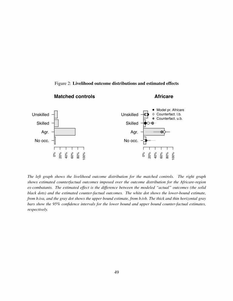
Figure 2: Livelihood outcome distributions and estimated effects

Matched controls

No occ.

Agr.

Skilled

Unskilled

0% 20%

40%

60%

80%

100%

Africare

No occ.

Agr.

Skilled

Unskilled

0% 20%

40%

60%

80%

100%

Model pr. AfricareCounterfact. l.b.Counterfact. u.b.

The left graph shows the livelihood outcome distribution for the matched controls. The right graphshows estimated counterfactual outcomes imposed over the outcome distribution for the Africare-regionex-combatants. The estimated effect is the difference between the modeled “actual” outcomes (the solidblack dots) and the estimated counter-factual outcomes. The white dot shows the lower-bound estimate,from b.iva, and the gray dot shows the upper bound estimate, from b.ivb. The thick and thin horizontal graybars show the 95% confidence intervals for the lower bound and upper bound counter-factual estimates,respectively.

49