1

Reinforcing Power Grid Transmissionwith FACTS Devices

Vladimir Frolov(1,4), Scott Backhaus (2,4) and Misha Chertkov (3,4,1)

(1) Skolkovo Institute of Science and Technology, 100 Novaya Str, Skolkovo 143025, Russia(2) Material Physics and Applications Division, LANL, Los Alamos, NM 87545, USA

(3) Center for Nonlinear Studies and Theoretical Division, LANL, Los Alamos, NM 87545, USA(4) New Mexico Consortium, Los Alamos, NM 87544, USA

Abstract—We explore optimization methods for planning theplacement, sizing and operations of Flexible Alternating CurrentTransmission System (FACTS) devices installed into the gridto relieve congestion created by load growth or fluctuationsof intermittent renewable generation. We limit our selection ofFACTS devices to those that can be represented by modification ofthe inductance of the transmission lines. Our master optimizationproblem minimizes the l1 norm of the FACTS-associated induc-tance correction subject to constraints enforcing that no line ofthe system exceeds its thermal limit. We develop off-line heuristicsthat reduce this non-convex optimization to a succession ofLinear Programs (LP) where at each step the constraints arelinearized analytically around the current operating point. Thealgorithm is accelerated further with a version of the cuttingplane method greatly reducing the number of active constraintsduring the optimization, while checking feasibility of the non-active constraints post-factum. This hybrid algorithm solves atypical single-contingency problem over the MathPower PolishGrid model (3299 lines and 2746 nodes) in 40 seconds periteration on a standard laptop—a speed up that allows the sizingand placement of a family of FACTS devices to correct a large setof anticipated contingencies. From testing of multiple examples,we observe that our algorithm finds feasible solutions that arealways sparse, i.e., FACTS devices are placed on only a few lines.The optimal FACTS are not always placed on the originallycongested lines, however typically the correction(s) is made atline(s) positioned in a relative proximity of the overload line(s).

Index Terms—Power Flows, FACTS devices, Non-convex Op-timization

I. INTRODUCTION

Power grids are undergoing significant evolution, e.g. ex-periencing disturbances caused by fluctuating renewable gen-eration, aging infrastructure with high costs for replacementsor upgrades, and the continual growth and evolution of elec-trical loads. However, the basic operational functions of thegrid remains the same, e.g., to balance the generation andload in interconnected transmission grids while respecting thetransmission line constraints (among several other constraintsand stability limits). These issues contribute to the growinginterest [1], [2], [3], [4], [5], [6], [7], [8], [9], [10], [11], [12],[13], [14], [15] in utilizing a new class of smart transmission-grid devices known commonly as Flexible Alternating CurrentTransmission System (FACTS) devices [16], [17], [18], [19].Although FACTS devices can provide fundamentally newdegrees of flexibility to transmission grids, they are also

expensive (especially fast solid-state devices) and must bedeployed in ways that maximizes benefit to the overall system.

Congestion relief is one attractive application of FACTSdevices that can provide significant system benefit for limitedcapital investment. However, the non-local nature of powerflows over transmission networks makes it difficult to de-termine where and how large a FACTS device(s) to install.To fully extract the benefit of FACTS devices, one oughtto build in the control of FACTS devices into algorithmsfor optimal placement and sizing, i.e., formulate and solvea comprehensive FACTS planning and control problem thatconsiders the transmission system as a whole. This type of in-tegration is not entirely new, see e.g. [2], [3], [7], but a system-level approach to the problem is deemed difficult. Indeed, thesystem-wide optimization suffers, in general, from the “curseof dimensionality”—the effort to exactly compute resultsscales exponentially with the system size and the numberpossible FACTS locations. It is impractical to implement suchdirect approaches for large transmission systems consisting ofthousands of components. However, some new approaches,brought into the power systems from statistical physics [20],[21], [22] and optimization [23], [24], [25], [26], suggestedthat even seemingly difficult optimization problems can bemodified into formulations which are provably polynomial (oreven linear). Such modifications are not achievable in all cases,and one often must search for computationally efficient yetempirically accurate heuristics. We take the latter path in thismanuscript.

Planning/sizing and operation/control problems are nor-mally considered separately. Planning problems seek to placeFACTS devices and determine the required operational ranges.The planning problem is a strategic decision, which takes intoaccount multiple operational conditions extending over years.On the contrary the control problem seeks the best response tocurrent conditions or those expected within a relatively shortperiod of time. However different the two type of problemsmay seem, they may be approached in a unified principledmanner similar to an approached developed in in [27] forplacement of storage. In [27], storage devices where placedall nodes in the network, but with appropriate penalties orcosts on utilizing the storage. By simulating operations overan many different situations, the statistics of storage utilizationwere used to eliminate lightly used nodes in favor of the more

arX

iv:1

307.

1940

v1 [

mat

h.O

C]

8 J

ul 2

013

2

frequently utilized nodes. Repeating this process several times“manually” created sparse storage solutions with this externalprocedure. Forcing sparsity internal to the process turns theoptimization problem into a far more difficult mixed formula-tion with both discrete and continuous variables entering theformulation. However, recent results in compressed sensing[28] 1 suggest that adjustment of the optimization cost functionmay allow sparsity to be enforced implicitly while keeping theoptimization variables in the preferred continuous domain.

We seek to adapt some of the techniques discussed above tothe problem of placing, sizing, and operating FACTS devicesto relieve transmission congestion. Here, we consider twoways of imposing congestion. The first is uniform load growthby application of the same scale factor to all loads in thetransmission grid model. A simple measure of grid robustnessis the amount of load scaling that can be accommodated beforea transmission constraint is violated. Alternatively, the amountload scaling achievable can be used a method to distinguishbetween different potential upgrades to improvement gridperformance, i.e. the upgrade that enables a larger scaling isranked higher. There are many ways to improve the systemto accommodate load growth, however traditional solutionssuch as building new transmission lines or generators closeto load are becoming increasingly difficult—an environmentthat begins to favor FACTS devices with their the smallerfootprint and lack of emissions. In particular, FACTS thatare able to control power flows or modify the inductance ofthe transmission lines are particularly attractive because a fewwell-placed FACTS devices can be intelligently controlled toredistribute power flows and relieve congestion on many powerlines, potentially including lines remote the the FACTS devicesthemselves.

Throughout this manuscript, we consider uniform scalingas the measures of stress and system performance. Othermethods of imposing transmission-grid stress are fluctuationsof intermittent renewable generation and N−1 contingencies.Fluctuations of intermittent generation will elicit a responsefrom the controllable generators (via primary frequency con-trol and subsequently via secondary control/AGC). For largefluctuations or those with particulary unfortunate spatial con-figurations, the power flows driven by the response of thecontrollable generators may cause overloading of transmissionlines. A method for finding the set of the most probable fluctu-ations that cause failure have been described [20], [21], [30].Then, instead of uniform load growth, the set of instantonsmay be used to apply stress to the transmission grid. N − 1contingencies also apply stress to the system, and congestionin potential N − 1 networks is a typical factor leading toreduced capability of the actual system.

We model the FACTS device[17] as a continuous modifica-tion of the inductance of a transmission line. Such a model isdirectly applicable to thyristor-controlled series compensation(TCSC) devices that use a continuously controllable reactorin parallel with a bank of switchable capacitors[7]. Phase-shifting transformers with appropriate local controls may also

1See also [29] for some related discussion in the power system context.

be considered within this model. We seek to resolve thefollowing questions:

• Can a particular infeasible configuration(s) of genera-tion and load, i.e. a configuration that violates one ormore transmission network constraints, be corrected withFACTS devices?

• When such a correction is possible, what is the optimal(least “expensive”) set of FACTS devices that achievesthis goal?

These two questions are formulated as one non-convex opti-mization problem with the l1 norm of the inductance deviationvector as an objective and the thermal limits for all the trans-mission lines as constraints. We construct efficient heuristicalgorithms that resolve these questions in a computationally-efficient manner, and moreover, we empirically observe thatthe optimal solutions are always sparse, i.e. only few FACTSdevices are actually needed.

Layout of material in the rest of the paper is as follows.We pose the problem of optimal placement of the inductancecorrecting FACTS devices in Section II; describe solutionalgorithm in Section III; and discuss results of our experimentsin Section IV. Section V is reserved for summary of the results,conclusions and discussing the path forward.

II. OPTIMIZATION MODEL

Before considering the optimal placement and sizing ofFACTS devices, we first discuss a few preliminaries.

A. General Setting: Power Flow (PF) and Optimum PowerFlow (OPF)

The transmission grid is represented as a graph G = (V, E)consisting of a set of vertices V and a set of undirected edgesE . The graph is assumed fixed. The vector of transmission linesusceptances is β .

= (βab|{a, b} ∈ E), and it is this β that weassume is modified by FACTS devices and is the subject ofoptimization. The transmission lines have power flow limitsrepresented by the vector f .

= (fab = fba > 0|{a, b} ∈ E).The generators have over and under generation limits g .

=(ga|a ∈ V), g .

= (ga|a ∈ V). We split the set of nodesV = Vc ∪ Vu into controllable nodes (traditional generatorsparticipating in control or perhaps modern controllable loads)and uncontrollable nodes (traditional loads and renewablegenerators). In our notation, the number of vertexes and edgesis N = |V| and M = |E|, respectively.

The transmission grid power flows are computed usingthe DC approximation, i.e., (a) the resistance of transmissionlines can be ignored in comparison with the line inductance,(b) the normalized voltage magnitude is unity at all nodes,and (c) phase difference between neighboring nodes is small,although we will use an iterative approximation to relaxthis approximation. The relationship between phases θa and

3

powers pa consumed/injected at any node a becomes linear:

∀a ∈ V : pa =∑b∼a

βab(θa − θb) = (Lθ)a, (1)

Lab.=

∑c∼a βac, a = b;−βab, a 6= b, {a, b} ∈ E ;0, otherwise.

(2)

where, L .= (Lab = Lba|a, b ∈ E) is the N × N weighted

graph-Laplacian matrix. The total balance of the real power is∑a∈V pa = 0, and the phase vector θ = (θa|a ∈ V) is defined

up to a global shift.

In the rest of this manuscript, we find it convenientto express L as L(β) = ∇+ ∗ β ∗ ∇. Here, ∇ is the(2M) ∗ N rectangular matrix which generates a 2M vectorof phase differences across the undirected edges (a, b), i.e.,∑Nc=1∇(a,b);cθc = θa−θb. Also, β is a (2M)×(2M) diagonal

matrix with elements βab for both directed edges (a, b) and(b, a). Finally, ∇+ is the N × (2M) transpose of ∇.

The phase vector is then expressed as θ = L−1p whereL−1 is the pseudo-inverse of L. The pseudo-inverse is well-defined because, by construction, N − 1 eigenvalues of L arepositive with the final zero eigenvalue corresponding a uniformshift of θ. This ambiguity in the phase vector θ is customarilyresolved by fixing the phase at the slack node (often the largestgenerator in the system).

Our objective in this manuscript is to optimally use FACTSdevices to relieve transmission congestion caused by additionalstress applied to a base grid configuration either via loadgrowth or fluctuating generation or load. To ensure that our re-sults are not biased by a poor choice of the base configuration,we select this configuration by performing an optimal powerflow (OPF) calculation. Starting from a known or forecastedset of uncontrolled power injections pu = (pa|a ∈ Vu), wesolve the following DC-OPF problem:

minpc

∑a∈Vc

ca(pa); (3)

s.t. ∀{a, b} ∈ E :∣∣((β ∗ ∇) ∗ L−1 ∗ p)(a,b)∣∣ ≤ fab,

∀a ∈ Vc : ga ≤ pa ≤ ga,

where the cost of generation ca(pa) is a non-decreasingfunction of pa. In the expression inside the absolute value onthe left and side of the first set of constraints, p is understoodto be the N × 1 column vector of the pa, and this expressionreduces to βab(θa − θb), i.e. the DC approximation of thepower flow on transmission line (a, b). The slightly morecomplicated form in Eq. 3 will prove useful in the discussionof optimization over the FACTS devices. When consideringstress applied by uniform load growth, a DC-OPF could berun to re-optimize the controllable generation at each levelof load growth. Instead, we uniformly grow all generation bythe same scale factor that we use to grow loads. This waywe overload some lines and then we try to find the solution(fix the lines) by searching for optimal susceptances with ouralgorithm.

B. Stressing of the Optimal Solution

Assuming a feasible solution p∗ to the DC-OPF exists, oneway to measure the robustness of the solution/grid is to scaleall of the generation and loads by a constant factor α > 1 andtest to see if the solution still respects the constraints in Eq. 3,i.e., if

∀{a, b} ∈ E : α∣∣((β ∗ ∇) ∗ L−1 ∗ p∗){a,b}∣∣ ≤ fab. (4)

The critical α, i.e αc, is the smallest value of α where atleast one of the transmission line constraints in Eqs. (4) isviolated. A super-critical, infeasible grid configuration is thengiven by p(in) = αp∗ with α > αc. Note that we assume thesystem is only constrained by transmission congestion and thatgeneration constraints do not play a significant role.

A second way to stress the solution p∗ to achieve aninfeasible p(in) is to choose certain configurations [20], [21]of the uncontrolled fluctuating generation and loads pu that,when combined with the response of the controlled generatorspc participating in secondary frequency control, results inviolations of transmission line constraints. Much like theuniform scaling discussed above, a one-dimensional family ofp(in) can be generated by scaling the original pu fluctuation.

C. Problem Formulation

We seek to improve the grid robustness to stress (e.g.,increasing the value of αc) by optimally placing FACTSdevices. Stress can be applied to the base grid configurationp∗ in many ways to create an infeasible p(in), including thetwo discussed above. However, the problem formulation thatfollows is independent how the stress applied.

In this initial work, we only consider FACTS devices whoseeffect can be approximated as modifying the susceptance(inductance) of a transmission line. Such FACTS devicesare expensive, and we incorporate this via the cost functionH(β;β(in)), where β(in) and β are the vectors of susceptancefor the infeasible solution and for the solution after FACTSmodifications. We model H(β;β(in)) as the l1-norm of theFACTS-induced change in β and pose the following optimiza-tion problem:

minβ

∑{a,b}∈E

|βab − β(0)ab | (5)

s.t. ∀{a, b} ∈ E :∣∣∣((β ∗ ∇) ∗ (L(β))−1 ∗ p(in))ab∣∣∣ ≤ fab.

In spite of some useful features of the dependence of thegraph-Laplacian on β, see e.g. [31], the nonlinear conditionsin Eq. (5) are generally non-convex in β. (See Appendix V-Awhere the non-convexity is illustrated on a three node exam-ple.) We resolve this complication in Section III by designinga greedy but efficient heuristic algorithm that enables solutionof (5) over large practical instances.

Eq. (5) is not guaranteed to have a feasible solution, i.e.FACTS corrections of line inductance may not be sufficient tocorrect all constraint violations when the system is severelystresses. It is interesting to discover the amount of stress toreach this second critical boundary. For case of uniform scaling

4

in Section II-B, we seek to find the α′c > αc such that p(in) =α′cp∗ results in infeasibility of Eq 5. This analysis will be

discussed on examples in Section IV.Finally, we note that is does not make sense to apply (5)

to radial distribution grids because, when G is a tree, fixing pleads to an unambiguous, β-independent set of power flows.However, even in the simplest case of a single loop theoptimization problem (5) becomes interesting and nontrivial(see discussion of Appendix V-A).

D. Critical Discussion

Before discussing implementation details in Section III), wefirst comment on the assumptions and limitations, but alsoadvantages, natural generalizations and uses of the FACTSplacement problem stated in Eq. (5). The following basicassumptions/caveats were used in the formulation of Eq. (5)

(1) The power flow equations are linearized, i.e. we use theDC approximation.

(2) The `1−norm cost function in Eq. (5) is over-simplifiedas it does not include fixed costs of installing FACTS thatdo not scale with β − β(in).

(3) Sparsity of FACTS placement is a desirable property ofany solution of Eq. (5), but sparsity is not explicitlyencouraged by the formulation.

(4) Generation constraints ga

and ga are ignored.(5) Only a single configuration p(in) is considered as a

guidance for FACTS installation.(6) The FACTS-corrected network is not guaranteed to be

N −1 reliable (or reliable with respect to a more generallist of contingencies).

We comment of these items in order.(1) Linearizing the power flow equations is advantageous as

it allows us to express the transmission-line thermal constraintswith an analytic formula in terms of β. Generalization to theexact nonlinear power flows is straightforward, however in thiscase getting an explicit formula for the line flows in terms ofβ may be a challenge. The lack of an explicit formula compli-cates the efficient computation of the β-derivative and iterativelinearization over β used to derive an efficient algorithm inSection III. A viable alternative for the exact nonlinear powerflow equations is iterative linearization over both susceptanceand phase angles around a base-solution.

(2) The choice of the l1 norm is illustrative. Many othercost functions may be incorporated without creating significantcomplications, including those with graph-inhomogeneity thatencourage building new FACTS at specific locations.

(3) Although we not to explicitly encourage sparsity, ourexperiments with large networks (see Section IV) naturallyresult in sparse solutions. We conjecture that the l1 norm maypromote sparsity in ways similar those in compressive sensing[28].

(4) Generalization of Eq. (5) accounting for generationlimits is straightforward.

(5) We have developed efficient algorithms for solvingEq. 5 so that we may simultaneously consider many different

stressed configurations by simply replicating Eq. 5. Specifi-cally, we create n replicas of the constraints in Eq. (5) forn different stressed configurations, p(1), · · · p(n), replacing Mconstraints in Eq. (5) by n∗M conditions and minimizing thecost function in Eq. (5) over the extended set of constraints.

(6) N − 1 reliability can be incorporated using methodssimilar to (5) above. Specifically, for a “virtual grid” witha one line disconnected (but the other M − 1 lines stillfunctioning), we derive the set of M − 1 constraints thatare explicitly dependent on all but one component of β. Wecombine all the constraints into a set of (M−1)∗M constraintswhich, additional to M base constraints, must be satisfied bya solution of Eq. (5).

The optimization problem (5), and its generalizations brieflydiscussed above, can be used both for planning of newFACTS installations into existing grid and for controllingexisting FACTS devices. In the case of planning, the list ofcontingencies p(1), · · · p(n) could include a number of differentconfigurations of a future stressed grid (including N − 1contingencies) for both the system peak and minimum. Thesolution of (5), if it exists, would then provide the lowest costplacement and sizing of FACTS that would resolve all of thenetwork constraint violations for the stressed configurationsconsidered. In the case of operations and control, contingen-cies may be considered one by one, e.g. a single N − 1contingency or one of the worst-case instantons discussed in[20], [21]. Equation (5) then enables a reactive control thatquickly computes the FACTS set points to maintain a feasiblesolution.

III. OPTIMIZATION ALGORITHM

Eq. (5) presents two challenges: the inequality constraintsare nonlinear and (b) there are too many constraints – thou-sands for a large transmission grid like that discussed inSection IV. In Sections III-A and III-B, we will describe waysovercome these challenges independently, and in Section III-Cpresent a synthesis strategy combines the two approaches intoone iterative procedure.

A. Linearization of Constraints

We take advantage of the explicit expression of the condi-tions in Eq. (5) and linearize these around the current valueof β∗,

∀{a, b} ∈ E : ((β ∗ ∇) ∗ (L(β))−1 ∗ p(1))ab≈ Aab(β∗) +

∑{c,d}∈E

(βcd − β∗cd)Bab;cd(β∗). (6)

The M-dimensional vector A and (M ×M) matrix B can bepre-computed explicitly (or tabulated in more general case)for a range of values of β∗. The resulting Sequential LinearProgramming (SLP) [32] approximate iterative algorithm thenbecomes

Direct Algorithm

• Start: k = 0. Initiate with β(0) = β(in).

5

• Step 1: Linearize conditions in Eq. (5) about β(k) ac-cording to Eq. (6) and solve the following LP, β(k+1) =

argminβ∑{a,b}∈E

|βab − β(0)ab | (7)

s.t. ∀{a, b} ∈ E :∣∣∣∣∣Aab(β(k))+∑{c,d}∈E

(βcd−β(k)cd )Bab;cd(β

(k))

∣∣∣∣∣ ≤ fab,• Step 2: If |β(k+1) − β(k)| is larger than a convergence

tolerance, then set k = k + 1 and go to Step 1.• End: Output β(k+1) as the solution.

Note that in actual experiments discussed in Section IV, thealgorithm converges after a small number of iterations withβ(k+1) exactly equal to β(k).

B. Cutting Plane

One problem with the optimization in (5) and the LPreformulation in Eq. (7) is the complexity due to the largenumber of constraints. However, in practical cases, very fewof these constraints are actually violated, suggesting thatthe complexity of the brute force implementation can bedrastically reduced with standard cutting-plane algorithms, seee.g. [33], [34]. A modification of Eq. (7) consists of cuttingthe constraints in two groups, “included” and “excluded”,and updating the two groups till convergence is reached.Initially, the included group consists of the constraints whichare violated for β = β(k), while all other constraints are placedin the excluded group. At every step of the inner iteration (withrespect to the algorithm explained in Section III-A), we solveEq. (7) using only the included constraints, and then check ifany of the excluded constraints are violated in the resultingsolution. If no excluded constraints are newly violated, weconclude that an optimal solution of the full problem is found.Otherwise, we pick the most violated constraint and move itfrom the excluded group to the included group and repeat. Thissimple and straightforward procedure works very effectivelyin all the practical cases we tested, normally stopping in lessthan a handful of steps.

C. Synthesis

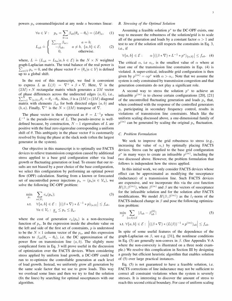
Our numerical experiments suggest that the algorithms per-formance can be boosted significantly by alternating the outer-loop LP solution with the inner-loop cutting plane, instead ofwaiting for convergence of the inner-loop cutting plane step:Improved Algorithm

• Start: k = 0. Initiate with β(0) = β(in). Split the listof 2M inequality constraints in Eq. (5)in to the included(E(in)) and excluded (E(out) = E \ E(in)) groups.

• Step 1a: Linearize the E(in) Eq. (5) about β(k) and solvethe following LP, β(k+1) =

argminβ∑{a,b}∈E

|βab − β(0)ab | (8)

s.t. ∀(a, b) ∈ E(in) : fab ≥

σab

(Aab(β

(k))+∑{c,d}∈E

(βcd−β(k)cd )Bab;cd(β

(k))

),

where σab is +1 or −1 depending on the signature of therespective directed (one-sided) inequality.

• Step 1b: Update E(in) moving all the currently violatedconstraints that are in E(out) for β(k) to E(in).

• Step 2: If |β(k) − β(k)| is larger than tolerance or if theupdate set on the previous step was not empty, then setk = k + 1 and go to Step 1a.

• End: Output β(k+1) as the solution.

Fig. 1. Flowchart of the improved algorithm. Multicore procedures aremarked. The most time consuming procedure is ”Solve LP”.

It is straightforward to verify that the fixed point of thisimproved algorithm procedure will also be a fixed point ofthe direct algorithm procedure (wait till convergence of theinner loop before making the next outer loop step). Giventhe global non-convexity of Eq. (5) potential landscape, oneobviously cannot guarantee that the fixed point of the improvedprocedure will always coincide with a fixed point of the directprocedure. However, the improved procedure is as good as thedirect one for finding a local minimum — which is exactlythe problem we are aiming to solve.

6

IV. EXPERIMENTS

Next, we illustrate the algorithms of Section III on twotransmission grids. The first is a 30-bus model from thesoftware Matpower [35] 2 (see Fig. 3), a small enough gridthat we can develop some intuition about how the FACTS arebeing utilized. The second is the Polish grid where we considertwo versions – a 2737-bus summer grid and a 2746-bus wintermodel (also available in Matpower, see Fig. 5). Tests of theimproved algorithm of Section III-C revealed that the numberof iterations required for convergence is unexpectedly small– less than a dozen for all the cases we experimented with(analysis of convergence is shown in the Fig.2). In the caseof the Polish grid, each iteration of our algorithm took 30seconds on a standard quad-core processor.

Fig. 2. Convergence of the cost with iteration step for 30-bus model (bluegraph) and for the Polish model (red graph).

The FACTS placements selected by the solutions of thenumerical experiments also revealed a number of interestingfeatures of the solutions that we discuss below.

A. Non-locality

The nonlocal behavior is illustrated on two examples of the30-node model with α/αc = 1.4 (40% overload) in Fig. 3 andα/αc = 1.9 (90% of overload) in Fig. 4. Initially overloadedlines are marked in red and modified lines are marked ingreen. The numbers near the modified lines are percentageof the susceptance change. Very often, although not always,our algorithm chose NOT to decrease the susceptance of theoverloaded lines to restrict the power flow on them, but insteadit modifies the susceptance of nearby lines to reroute powerflows around the congested transmission lines. This ratherfrequent nonlocal behavior of the optimal solutions suggeststhat the optimal placement of FACTS devices is nontrivialproblem and calls for a computationally efficient approach,

2To convert MatPower cases into the standard format (matrix L and vectorp), transformers and phase shifters are turned off, double lines are combinedto form one line with value of throughput and inductance calculated from twolines. Double generators also were combined to form one generator.

such as the one we consider here, so that the method can beapplied to much larger grids as well.

Arrowheads on the lines in Fig. 4 indicate the directionthe original α/αc = 1.9 power flows and the smaller arrows(green/down or red/up) indicate whether the original powerflows decreased or increased after the FACTS were placed.The original power flows out of generator G1 overloaded lineL1. Our algorithm drives β → 0 on line L4 and increasesβ on line L2 effectively rerouting the power from G1 to thelower right of the network. The increase in power flow on L2also relieves the overload on L3 demonstrating the inherentlynon-local effects of FACTS. This redistribution of power flowshas even longer range effects. The major reduction of flow online L4 has two other beneficial impacts. First, it draws morepower from G2 (in spite of the decrease in β on L5) relievingthe overload on L6. In addition, it forces a reversal of thepower flow on line L7 relieving the overload on L8.

The small test grid in Fig. 4 enables us to build up someintuition about the non-local effects that affect the optimalplacement and sizing of FACTS. We next consider the sameuniform load scaling for the much larger Polish grid. Fig-ure 5 highlights the small region of the Polish grid whereall of the overloads and susceptance modifications occur forα/αc = 1.38. The results are presented in the tabular form fordifferent values of α/αc in Fig. 6 and demonstrate behaviorsimilar to the much smaller 30-bus network. For small α/αcup to at least 1.04, the optimal solution is local, i.e. ouralgorithm selects to simply reduce the susceptance of line375, which reduces the flow on this overloaded line. As α/αcgrows, non-local behavior becomes apparent. For α/αc ≥ 1.1,additional lines become overloaded, however, none of theselines are selected for susceptance modification. Interestingly,line 375, which was the initial overloaded line, is selected forsusceptance modification in all of the solutions.

The details of the highlighted region of Fig. 5 are shown inFig. 7 for α/αc = 1.38. The structure of the solution is similarto the 30-bus configuration one. The overloads are resolvedby changing the susceptances of the near lines to reorganizepower flows structure in the system. It can be seen that thecorrections are not always non-local. Here the 375th line wasoverloaded initially and also corrected in the solution.

We note that in some of the cases, our algorithm selectedsusceptance corrections that set a line’s total susceptanceto zero, i.e. corresponding to the removal of the line fromthe network. This curious fact was also verified directly bymanually removing the line in question and rerunning ouralgorithm. The resulting solution was indeed a valid solution(i.e. no lines overloaded). The structure of such solution isthe same. If we do not consider line 33 which was removed(shown in the Fig.4), the same lines were changed and thecorrections are approximately the same.

B. Sparsity

A second interesting observation concerns sparsity of theoptimal solution. Instead of requiring small modifications ofmany lines throughout the network, our algorithm makes

7

Fig. 3. Visualization of the 30-node model illustrating the non-locality ofthe optimal solution with α/αc = 1.40 yellow buses - loads, blue buses -generators. Lines marked in red were overloaded in the base case (two lines),while those marked in green where selected by our algorithm for susceptancemodification by FACTS devices (two lines). The percentage of the correctionto the susceptance is shown next to the corrected lines. The difference in powerflows through the lines after the corrections are shown with short green arrows(decrease of the flow) and short red arrows (increase of the flow). If there isno arrow then power flow is the same.

Fig. 4. Visualization of the 30-node model illustrating the non-locality ofthe optimal solution with α/αc = 1.90 yellow buses - loads, blue buses -generators. Lines marked in red were overloaded in the base case (four lines),while those marked in green where selected by our algorithm for susceptancemodification by FACTS devices (three lines). Directions of the in-line arrowsindicate directions of the flow prior to the FACTS corrections. The percentageof the correction to the susceptance is shown next to the corrected lines(susceptance of the 33th line is going to 0). The difference in power flowsthrough the lines after the corrections are shown with green short arrows(decrease of the absolute value of the flow) and red short arrows (increase ofthe absolute value of the flow). If there is no arrow then power flow is thesame. If power flow through the line changes the direction after installationof FACTS (corrections made) it is illustrated by dotted line (two lines).

significant susceptance modifications to a only few lines withthe number of modified lines typically the same or slightlysmaller than the number of overloads in the base case. This

Fig. 5. Non-geographical visualization of the entire Polish grid. Thehighlighted region contains all of the overloaded and FACTS-modified linesfor the cases shown in the table of Fig. 6. Part of the highlighted region isshown in more detail in Fig. 7 for α/αc = 1.38 with the red nodes herecorresponding to the big nodes of Fig. 7.

Fig. 6. Table showing which lines are overloaded in the base solution of thePolish grid in Fig. 5 for selected values of α/αc and lines selected by ouralgorithm for susceptance modification by FACTS. For α/αc ≤ 1.04, theoverload is relieved by simply lowering the susceptance on the overloadedline to limit the flow on that line. For larger α/αc, the solution becomenonlocal with the additional susceptance modifications placed on lines thatare not overloaded in the base solution.

behavior is qualitatively similar in examples of the 30-nodenetwork and of the Polish networks and can be seen inFigs. 3, 4, and 7. We note that our `1−norm cost functiondoes not explicitly promote sparsity, i.e. for a given budgetof susceptance modification, it does not cost more to spreadit out over the entire network rather than concentrate it on

8

Fig. 7. Detail of the highlighted region of the Polish grid from Fig. 5showing the lines overloaded in the base case (α =1.38) in red and thoseselected by our algorithm for susceptance modification in green. Generatorsare marked as blue and loads are as yellow nodes. The one line shown inblue was both overloaded and modified. The numbers labelling these linescorrespond to the line numbers in the table of Fig. 6. Although the Polishgrid is much larger, the behavior is very similar to that of the 30-node grid inFigs. 3 and 4, i.e. susceptances are primarily modified on lines that are nearto the originally overload lines to encourage the power flow to be reroutedaround the overloads to relieve congestion.

a few lines. However, the sparsity of the solution emergesnaturally. We conjecture that this sparsity is a natural propertyof the “N-1 redundancy” engineered into electrical networks,i.e. N-1 redundancy generally requires that there be at least twopaths to deliver power to loads, and if one of paths becomesoverloaded, an increase in susceptance of an alternate path willdeliver more power thus relieving the congestion on the firstpath 3. These observations suggest an additional cutting plane-like heuristic that could speed up our algorithm even further:instead of optimizing over the susceptances of all of the lines,one could restrict our attention to the set of lines that are nearto the overloaded lines.

C. Uniform Load Scaling and Emergence of Local Optima

By efficiently solving the optimization problem in Eq. 5, ouralgorithm allows a more thorough exploration of the solutionspace. In particular, we investigate the emergence of multipleminima of the cost function in Eq. 5 as we uniformly re-scalethe loads by α in both the 30-node and Polish networks.

For the 30-node network, Fig. 8 clearly shows a jump inthe cost at α = 1.51 signaling emergence of multiple (atleast two, but possibly more) local minima. Investigation ofthe details of the solutions above and below the jump showsthat the corrections to susceptances of lines #33 and #40 aresignificantly different. Above the jump, the net susceptance ofline #33 becomes approximately zero indicating that this linehas effectively been removed from the network. The results

3Even thought the sparsity was not enforced directly, the use of the l1 normin the cost function of Eq. (5) was most probably helping implicitly, similarlyto how the sparsity arises in compressed sensing, see e.g. [].

Fig. 8. Dependence of the optimal cost on the scaling factor, α, shown forthe working case of the 30 node model. Lines which were corrected and theirfinal susceptances are illustrated for lines #33, 36, 32 and 40.

Fig. 9. Dependence of the optimal cost on the scaling factor, α, shown forone of the summer cases of the Polish model. Lines which were corrected andtheir final susceptances are illustrated. Bends of the cost graph correspond tothe corrections of additional lines.

in Fig. 8 leads us to suspect that, by always initiating withthe base solution, our algorithm has become trapped in alocal minima for α < 1.51. To verify this suspicion, weinitiated the algorithm with a configuration equivalent to thebare configuration for all lines but with line #33 removed.Dependence of optimal cost of α for this case is illustratedin the Fig.10 with final susceptances of the lines shown.Assuming that turning the line off costs zero we significantlydecreased the cost of corrections. But the jump of the cost stillexists which means that we still have another minima of thecost function.

To prove the fact that there are more than one minima (morethan one final solutions for one initial configuration of thesusceptances) let us compare the initial solution (Fig.8) and thesolution with line #33 turned off (now we will calculate the

9

cost of such operation in terms of the cost function defined).Costs of two different solutions for the same initial grid (30-bus grid) are illustrated in the Fig.11.

Three regions can be seen in the graph. In the 3rd region,the solutions are the same. In the 1st region, there is extracost associated with the forced reduction of the susceptanceof line #33. This effective removal of line #33 does not resultin lower cost. But in the 2nd region it can be seen that thisremoval does decrease the final cost compared to a solutionwhere line #33 was not removed. There are two differentsolutions with different costs implying that at leats two minimaof cost function exist.

Fig. 10. Dependence of the optimal cost on the scaling factor, α, shown forthe working case of the 30 node model. Lines which were corrected and theirfinal susceptances are illustrated for lines #33, 36, 32 and 40. Line #33 wasturned off with zero cost.

Fig. 11. Comparison of the solutions given in the Fig. 8 and Fig. 10. Solutionsare evaluated in terms of the cost function defined above. Turning line #33off is not free now.

The same analysis (but no jumps in this case) for Polish caseis shown in the Fig.9. Different bends of the cost vs scalingfactor dependence seen in Fig. 9 also indicates competition

between different optimal structures. The structures are differ-ent in the number of overloaded lines, the number FACTS-corrected lines (Fig.6), and the magnitudes of the corrections.Indeed, at small α the optimal configuration contains oneoverloaded and one corrected line. At α ≈ 1.06, anotherline becomes overloaded, however the configuration is stillcorrectable with a single FACTS device positioned at the sameline as before. At α ≈ 1.26, another line becomes overheated,but it does not require an additional FACTS device untilα ≈ 1.29, etc.

D. Robust Optimal Placement: Correcting Multiple Configu-rations

Up to this point, we have only considered using FACTSto modify line susceptances to correct a single configurationthat causes network overloads. However, as discussed inSection II-D, we can easily robustly optimize the placementand sizing of FACTS to correct n configurations that leadto overloads. We modify the LP portion of the improvedalgorithm of Section III-C by extending the list of constraints.For each of the n network configurations, p(1), · · · p(n), onevery iteration step (Fig.1) we create a list of 2m(1), · · · 2m(n)

inequalities for the m(i) transmission lines from “included”and combine all these inequalities in one extended list. Wethen replace the list of the directed edge labels E in Eq. 5 withthe new composite list and iterate the improved algorithm asdescribed in Section III.

To demonstrate the effectiveness of this method, we con-sider a simple situation where we simultaneously optimizeFACTS placement and sizing over two supercritical cases. Thefirst case describes uniformly scaled Polish grid’s winter off-peak configuration from MatPower. The second case is gen-erated from the preceding configuration by adding a fractionX to the previous loads where X is distributed uniformlyfrom −0.7 to 0.7. Following the load changes, the secondconfiguration includes a generation adjustment via an optimalpower flow, and then the loads were uniformly scaled.

Fig. 12 shows the resulting cost of the robust optimization(green curve) compared to the optimal FACTS placement andsizing that only considers one or the other scenario (red andblue curves). Since the robust optimization is correcting bothoverloads at the same time, the total cost is higher than eitherthe red or blue curves. However, it is lower than the yellowcurve which is the sum of the maximum cost per line overthe two scenarios, i.e. the cost one would naively compute byoptimizing FACTS placement and sizing for the two scenariosindependently.

The advantage of the robust optimization is not observed inall cases. For example, if in the two scenarios the overloadedlines were spatially well separated, the lack of interaction be-tween the FACTS devices and transmission line constraints atthese locations would effectively split the robust optimizationback into two separate, uncoupled optimizations. A secondcase where the robust optimization does not improve theresults is when the scenarios have exactly the same set ofline overloads. However, if the lines that are overloaded in the

10

Fig. 12. Optimal cost vs scaling parameter shown for FACTS placementsover three different settings of Polish grid are marked in red, blue and greencolors. The result of optimization over a base, off-peak winter configurationis shown in red. The blue curve shows the optimization result for anotherconfiguration with the same line topology as in the base case, however withrandomly generated corrections to loads and respective OPF adjustment of thegeneration. The green curve shows robust-optimal FACTS placement whichoptimal of all placements which remain feasible for both, base and corrected,configurations. This green curve should be compared with naive combinationof the two single-configuration optimization shown in yellow.

different scenarios are in reasonable proximity, the FACTSdevices that correct one scenario may be leveraged to correctanother scenario at lower total cost. For the results displayedin Fig. 12, we have purposely picked a randomly-generatedsecond scenario that displays some overlap with the original,uniformly-scaled (α = 1.08) Polish winter base case.

V. CONCLUSIONS AND FUTURE WORKS

In this manuscript we studied how adjusting power lineinductances with FACTS devices can help to reduce congestionin the power systems. Our main finding is the suggestion ofefficient heuristics which can be used for both operational(short term) and planning (long term) purposes. The heuristicsare used in an algorithm that minimizes the deployment ofFACTS using an l1-norm as a measure FACTS cost. The min-imization is done under the condition that thermal overloadsare relieved for a specially selected bad configuration(s) ofload and generation. The algorithm performance is illustratedon moderate and large scale models. We find that the resultingoptimal FACTS deployments are sparse, i.e. necessary at onlya handful of lines. However, the lines to be corrected are notnecessarily lines with the most sever overload (without thecorrection applied).

There are number of directions for future work in this areaincluding:

• Incorporating in the operational scheme multiple danger-ous configurations and possibly including an outer stepto search for these configurations.

• Considering FACTS control in combination with otherdevices and controls, e.g. energy storage and generationre-dispatch.

• Extension of the planning paradigm to stochastic settingthat takes into account the statistics of multiple stressedconfigurations and considers the investment problem ofplacing and sizing FACTS devices to minimize risks.

• Generalize the model presented here to account for moregeneral (and accurate) AC modeling of power flows, thusmodeling risks of loss of synchrony and voltage collapse(in addition to the risk of the thermal overload discussedin this manuscript).

APPENDIX

A. Motivating Three Node Example

Fig. 13. The simple graph of the three node example.

Here we illustrate non-convexity of our general formulation(5) on the simple three node example of Fig. 13, wherea = 1, · · · , 3. Power flows are solved explicitly and then thedomain limited by six conditions in Eq. (5) is shown, as thefunction of three susceptances, β12, β13, β23, in Fig. 14, wherewe see clearly nonlinearity and non-convexity of the domain inβ. Fig. 15 illustrates our linearized algorithm (no need to addcutting plane trick here). Here, the exact optimization domain(equivalent to the one shown in Fig. 14 but rotated for betterview) is shown in red, and domain linearized around the basicβ0 case is shown in blue. Two red points mark initial state(outside of the domains) and final optimal state (inside of thedomains) found in one iteration.

B. Sensitivity of Line Flow to Local Change of Susceptance

It is instructive to analyze sensitivities of the line flows tochanges of the line suspectances on this simple three nodeexample. Power flow over a line of the triangle, say line (1, 2),is

p12 =β12(p1β23 − p2β13)

β12β13 + β12β23 + β13β23, (9)

where pi is the production/consumption at the node i (whichis positive/negative). Then the sensitivity of the flow to the

11

Fig. 14. Visualization of the three dimensional β space for the three nodeexample of Fig. 13. Non-convexity of the domain is clearly seen.

Fig. 15. The three dimensional β space as in Fig. 14 but rotated. Red areamarks feasible domain of the original nonlinear conditions in (5) for the threenode example, and blue area corresponds to its linearized version as in Eq. (7).Red dots stand for the initial, β0, configuration (seen outside of the domains),and the final solution (inside of the domains) achieved in one iteration of thedirect algorithm of Section III-A.

change of susceptance at the same or neighboring lines (underfixed nodal productions/consumptions) becomes

∂p12∂β12

=β13β23p12

β12 (β12β13 + β12β23 + β13β23)(10)

∂p12∂β23

=β12β13p23

β23 (β12β13 + β12β23 + β13β23). (11)

From these formulas (and also taking into account that all thesuscpetances are positive) one concludes that in order to reducethe value of the flow over a line, in the case when correction

of only a single line susceptance is allowed, one either (a)decreases susceptance of the same line which is overloaded,or (b) increases/decreases susceptance of the neighboring linedepending on if the directions of the original and neighboringline flows towards their common point are the same/different.(The “same” and “different” are interpreted as → · ← and→ · →, respectively.)

ACKNOWLEDGMENT

The work at LANL was carried out under the auspicesof the National Nuclear Security Administration of the U.S.Department of Energy at Los Alamos National Laboratoryunder Contract No. DE-AC52-06NA25396. This material isbased upon work partially supported by the National ScienceFoundation award # 1128501, EECS Collaborative Research“Power Grid Spectroscopy” under NMC.

REFERENCES

[1] M. Noroozian, L. Angquist, M. Ghandhari, and G. Andersson, “Use ofupfc for optimal power flow control,” Power Delivery, IEEE Transac-tions on, vol. 12, no. 4, pp. 1629 –1634, oct 1997.

[2] D. Gotham and G. Heydt, “Power flow control and power flow studiesfor systems with facts devices,” Power Systems, IEEE Transactions on,vol. 13, no. 1, pp. 60 –65, feb 1998.

[3] S. Gerbex, R. Cherkaoui, and A. Germond, “Optimal location of multi-type facts devices in a power system by means of genetic algorithms,”Power Systems, IEEE Transactions on, vol. 16, no. 3, pp. 537 –544, aug2001.

[4] A. Oudalov, R. Cherkaoui, and A. Germond, “Application of fuzzylogic techniques for the coordinated power flow control by multipleseries facts devices,” in Power Industry Computer Applications, 2001.PICA 2001. Innovative Computing for Power - Electric Energy Meets theMarket. 22nd IEEE Power Engineering Society International Conferenceon, 2001, pp. 74 –80.

[5] T. Orfanogianni and R. Bacher, “Steady-state optimization in powersystems with series facts devices,” Power Systems, IEEE Transactionson, vol. 18, no. 1, pp. 19 – 26, feb 2003.

[6] W. Wu and C. Wong, “Facts applications in preventing loop flows ininterconnected systems,” in Power Engineering Society General Meeting,2003, IEEE, vol. 1, july 2003, p. 4 vol. 2666.

[7] G. Glanzmann and G. Andersson, “Using facts devices toresolve congestions in transmission grids,” in CIGRE/IEEEPES, 2005. International Symposium, oct. 2005, pp. 347 –354. [Online]. Available: \url{http://www.eeh.ee.ethz.ch/uploads/txethpublications/Glanzmann CIGRE 05.pdf}

[8] W. Shao and V. Vittal, “Lp-based opf for corrective facts controlto relieve overloads and voltage violations,” Power Systems, IEEETransactions on, vol. 21, no. 4, pp. 1832 –1839, nov. 2006.

[9] M. Santiago-Luna and J. Cedeno-Maldonado, “Optimal placement offacts controllers in power systems via evolution strategies,” in Trans-mission Distribution Conference and Exposition: Latin America, 2006.TDC ’06. IEEE/PES, aug. 2006, pp. 1 –6.

[10] K. Lee, M. Farsangi, and H. Nezamabadi-pour, “Hybrid of analyticaland heuristic techniques for facts devices in transmission systems,” inPower Engineering Society General Meeting, 2007. IEEE, june 2007,pp. 1 –8.

[11] C. Rehtanz and U. Hager, “Coordinated wide area control of facts forcongestion management,” in Electric Utility Deregulation and Restruc-turing and Power Technologies, 2008. DRPT 2008. Third InternationalConference on, april 2008, pp. 130 –135.

[12] H. Sauvain, M. Lalou, Z. Styczynski, and P. Komarnicki, “Optimal andsecure transmission of stochastic load controlled by wacs #x2014; swisscase,” in Power and Energy Society General Meeting - Conversion andDelivery of Electrical Energy in the 21st Century, 2008 IEEE, july 2008,pp. 1 –5.

[13] Q. Wu, Z. Lu, M. Li, and T. Ji, “Optimal placement of facts devices by agroup search optimizer with multiple producer,” in Evolutionary Com-putation, 2008. CEC 2008. (IEEE World Congress on ComputationalIntelligence). IEEE Congress on, june 2008, pp. 1033 –1039.

12

[14] J. Filho, N. Martins, and D. Falcao, “Identifying power flow controlinfeasibilities in large-scale power system models,” Power Systems, IEEETransactions on, vol. 24, no. 1, pp. 86 –95, feb. 2009.

[15] M. Sahraei-Ardakani and S. Blumsack, “Market equilibrium for dis-patchable transmission using fact devices,” in Power and Energy SocietyGeneral Meeting, 2012 IEEE, 2012, pp. 1–6.

[16] F. ac transmission systems (FACTS), “http://en.wikipedia.org/wiki/Flexible AC transmission system.”

[17] “Proposed terms and definitions for flexible ac transmission system(facts),” Power Delivery, IEEE Transactions on, vol. 12, no. 4, pp. 1848–1853, oct 1997.

[18] N. Hingorani and L. Gyugyi, Understanding FACTS concepts andtechnology of flexible AC transmission systems. IEEE Press, New York,2000.

[19] R. Mathur and R. Varma, Thyristor-based FACTS controllers for elec-trical transmission systems. IEEE Press, Piscataway, 2002.

[20] M. Chertkov, F. Pan, and M. Stepanov, “Predicting failures in powergrids: The case of static overloads,” IEEE Transactions on Smart Grids,vol. 2, p. 150, 2010.

[21] M. Chertkov, M. Stepanov, F. Pan, and R. Baldick, “Exact and efficientalgorithm to discover extreme stochastic events in wind generation overtransmission power grids,” CDC-ECC, pp. 2174 –2180, dec. 2011.

[22] F. Dorfler, M. Chertkov, and F. Bullo, “Synchronization in ComplexOscillator Networks and Smart Grids,” Proceedings of NationalAcademy of Sciences, vol. 10.1073/pnas.1212134110, 2013. [Online].Available: \url{http://arxiv.org/abs/1208.0045}

[23] J. Lavaei and S. Low, “Zero duality gap in optimal power flow problem,”IEEE Transactions on Power Systems, 2012.

[24] D. Bienstock, M. Chertkov, and S. Harnett, “Chance Constrained

Optimal Power Flow: Risk-Aware Network Control under Uncertainty,”http://arxiv.org/abs/1209.5779, 2012. [Online]. Available: \url{http://arxiv.org/abs/1209.5779}

[25] S. Bose, D. Gayme, K. M. Chandy, and S. Low, “Quadratically con-strained quadratic programs on acyclic graphs with application to powerflow,” in arXiv:1203.5599, 2012.

[26] C. Coffrin, P. van Hentenryck, and R. Bent, “Approximating linelosses and apparent power in ac power flow linearizations,” in PowerEngineering Society General Meeting 2012, 2012, pp. 1–8.

[27] K. Dvijotham, S. Backhaus, and M. Chertkov, “Operations-Based Plan-ning for Placement and Sizing of Energy Storage in a Grid With a HighPenetration of Renewables,” ArXiv e-prints, Jul. 2011.

[28] E. J. Candes, M. B. Wakin, and S. Boyd, “Enhancing sparsity byreweighted l1 minimization,” Journal of Fourier Analysis and Appli-cations, vol. 14, no. 5, pp. 877–905, 2008.

[29] J. Johnson and M. Chertkov, “A majorization-minimization approachto design of power transmission networks,” in Decision and Control(CDC), 2010 49th IEEE Conference on, dec. 2010, pp. 3996 –4003.

[30] S. Baghsorkhi and I. Hiskens, “Analysis tools for assessing the impactof wind power on weak grids,” SysCon, pp. 1 –8, march 2012.

[31] A. Ghosh, S. Boyd, and A. Saberi, “Minimizing effective resistance ofa graph,” SIAM Review, vol. 50, no. 1, pp. 37–66, 2008.

[32] S. L. Programming, “http://en.wikipedia.org/wiki/Successive linearprogramming.”

[33] D. P. Bertsekas, Nonlinear Programming. Athena Scientific, 1999.[34] M. Avriel, Nonlinear Programming: Analysis and Methods. Dover

Publications, 2003.[35] [Online]. Available: http://www.pserc.cornell.edu/matpower/