Reineke’s Stand Density Index: Where Are We and Where Do We Go From Here?

John D. Shaw USDA Forest Service, Rocky Mountain Research Station

507 25th Street, Ogden, UT 84401 jdshaw@fs.fed.us

Citation: Shaw, J.D. 2006. Reineke’s Stand Density Index: Where are we and where do we go from here? Proceedings: Society of American Foresters 2005 National Convention. October 19-23, 2005, Ft. Worth, TX. [published on CD-ROM]: Society of American Foresters, Bethesda, MD.

REINEKE’S STAND DENSITY INDEX: WHERE ARE WE AND

WHERE DO WE GO FROM HERE?

John D. Shaw USDA Forest Service

Rocky Mountain Research Station Forest Inventory and Analysis

507 25th Street Ogden, UT 84401

Email: jdshaw@fs.fed.us

Abstract: In recent years there has been renewed interest in Reineke’s Stand Density Index (SDI). Although originally described as a measurement of relative density in single-species, even-aged stands, it has since been generalized for use in uneven-aged stands and its use in multi-species stands is an active area of investigation. Some investigators use a strict definition of SDI and consider indicies developed for mixed and irregularly structured stands to be distinct from Reineke’s. In addition, there is ongoing debate over the use of standard or variable exponents to describe the self-thinning relationship that is integral to SDI. This paper describes the history and characteristics of SDI, its use in silvicultural applications, and extensions to the concept. Keywords: Stand Density Index, self-thinning, density management diagrams, silviculture, stand dynamics

2

INTRODUCTION Silviculturists have long sought, and continue to seek, simple and effective indicies of competition in forest stands. Reineke’s Stand Density Index (SDI) (Reineke 1933) is one such index that is commonly used in North America and is being adopted elsewhere (e.g., Vacchiano et al. 2005). Reineke (1933) examined size-density data for 14 forest types – pure and mixed composition, natural stands and plantations – and concluded that when the log of quadratic mean diameter was plotted against the log of stem density (trees per acre), the maximum values formed a slope that was consistent among species (equation 1). Although the slope appeared to be constant, the intercept varied among species. When the intercept is located such that all size-density points fall below the curve, the curve represents the maximum size-density relationship for the species or forest type. [1] kDN +−= log605.1log where N = number of trees per acre, D = diameter at breast height k = constant varying with species For any stand, relative density could be described in two ways. In the first, the maximum size-density curve represents 100% density and other size-density combinations are expressed as a percentage of the maximum. Because the maximum varied by species, Reineke suggested an alternative in which all size-density combinations were referenced in terms of equivalence to the number of 10-inch stems per acre. In practice, both methods are useful – in the former case, the density of a stand can be assessed in terms of the maximum possible for its type, and in the latter, the density of stands of differing composition may be compared to a common reference. Reineke’s SDI is the latter case, which is calculated directly using equation [2].

[2] 605.1

10⎟⎠⎞

⎜⎝⎛=

DqTPASDI

where TPA is the number of trees per acre, Dq is quadratic mean diameter in inches. It should be noted that in metric units, 25cm is conventionally used in the denominator rather than a strict conversion of inches to centimeters (i.e., 25.4cm). As such, English and metric SDI values are not directly convertible (Daniel et al. 1979). Reineke found conformity in the slopes of 12 of the 14 forest types he examined. He described slash pine as a “possible” non-conformer and shortleaf pine as a “definite” non-conformer, but speculated that site factors, rather than an inherent difference in species characteristics, might be responsible for the observed patterns. In the case of shortleaf pine, Reineke speculated that frequent fire could be a reason for a different slope. For a given forest type Reineke found “no appreciable correlation” between SDI and age or site quality. In other words, a species’ slope and intercept, and therefore, maximum SDI, was expected to be invariant across its range. For these reasons, as well as some advantages to using SDI over basal area as a competition index (Zeide 2005), SDI has become the preferred stocking index for many practitioners.

3

SDI in APPLICATION The extent to which Reineke’s SDI was used in the 30 to 40 years following publication is not well known. Reineke’s work was mentioned briefly in contemporary silviclture and mensuration texts (Baker 1934; Bruce and Schumacher 1942). Meyer (1953) states that although Reineke’s stand density index is “relatively new”, it “is used in most American yield tables of recent date”. Such being the case, SDI may have been used implicitly by many practitioners in the form of yield tables, and not explicitly using the graphical tool presented by Reineke (1933). In the 1950s and early 1960s, Japanese scientists explored the size-density relationship experimentally (Kira et al. 1953; Shinozaki and Kira 1956; Yoda et al. 1963), establishing the so-called -3/2 self-thinning rule. The size-density relationship was incorporated into density management diagrams (DMDs) (Ando 1962, 1968), which graphically depict relative density and stand dynamics. Density management diagrams were introduced to the English literature by Drew and Flewelling (1977, 1979). In their diagram, Drew and Flewelling (1979) correlated percentages of stand density with benchmarks of stand development. Density management diagrams have taken various forms and provide silviculturists with a convenient tool for assessing stand density and planning interventions (for more on DMDs, see Jack and Long 1996, Newton 1997). At the same time that density management diagrams were enjoying increased use and acceptance, some questioned the validity of the self-thinning rule as an ecological “law” (e.g., Weller 1987; Osawa and Sugita 1989; Weller 1990; Sackville Hamilton et al. 1995), and doubt was raised over the constancy of the self-thinning slope among species. Various approaches to evaluation of the slope have been used, but all appear to have limitations or allow for some degree of subjectivity. Reineke (1933) used a subjective approach, drawing a line tangent to size-density data from a large number of stands. The approach taken by Japanese scientists (e.g. Kira et al. 1953; Shinozaki and Kira 1956; Yoda et al. 1963) – remeasurements of self-thinning populations – provided relatively convincing support for the establishment of the self-thinning rule but, in general, their methods were difficult to apply to forest trees. However, forest remeasurement data have been used, including some very long records (Pretzsch and Biber 2005). Accurate determination of the self-thinning trajectory for any population remains a difficult task, whatever the data source. Some of the problems are inherent in the data, especially those obtained using temporary plots. First, in a given sample only a fraction of stands are actually in a true self-thinning mode. The rest are less than optimally stocked for a number of reasons. For example, it is uncommon to find stands regenerated at sufficient density such that they are at maximum relative density at young ages. In older stands, insects, disease, and other disturbances may reduce stocking more rapidly than the residual stand is able to re-occupy growing space. In both cases it is necessary to censor the data or apply methods that are insensitive to observations in understocked conditions. Although some work has been done to address these problems (e.g., Leduc 1987, Bi and Turvey 1997, Bi et al. 2000), limitations persist. Given the difficulty of determining the “true” self-thinning trajectory, one might ask whether it is productive to continue debate over the universality of the self-thinning slope among species. One answer might be that the phenomenon is real, but simply not observable because of the

4

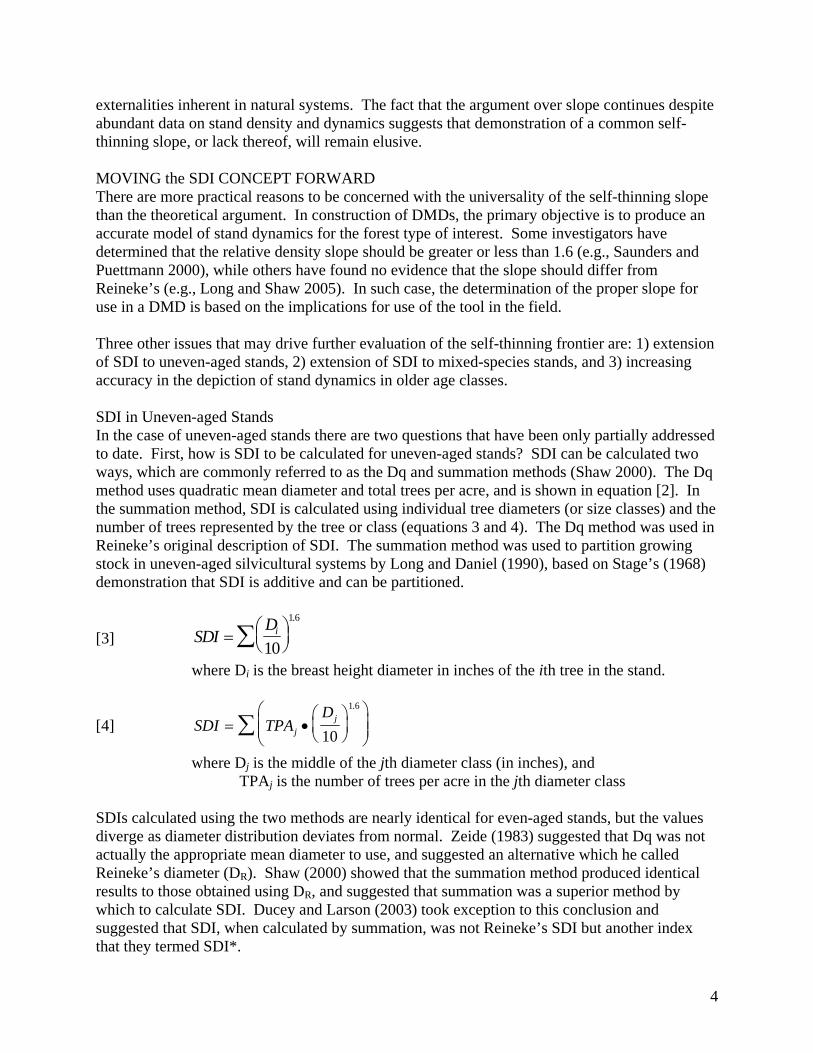
externalities inherent in natural systems. The fact that the argument over slope continues despite abundant data on stand density and dynamics suggests that demonstration of a common self-thinning slope, or lack thereof, will remain elusive. MOVING the SDI CONCEPT FORWARD There are more practical reasons to be concerned with the universality of the self-thinning slope than the theoretical argument. In construction of DMDs, the primary objective is to produce an accurate model of stand dynamics for the forest type of interest. Some investigators have determined that the relative density slope should be greater or less than 1.6 (e.g., Saunders and Puettmann 2000), while others have found no evidence that the slope should differ from Reineke’s (e.g., Long and Shaw 2005). In such case, the determination of the proper slope for use in a DMD is based on the implications for use of the tool in the field. Three other issues that may drive further evaluation of the self-thinning frontier are: 1) extension of SDI to uneven-aged stands, 2) extension of SDI to mixed-species stands, and 3) increasing accuracy in the depiction of stand dynamics in older age classes. SDI in Uneven-aged Stands In the case of uneven-aged stands there are two questions that have been only partially addressed to date. First, how is SDI to be calculated for uneven-aged stands? SDI can be calculated two ways, which are commonly referred to as the Dq and summation methods (Shaw 2000). The Dq method uses quadratic mean diameter and total trees per acre, and is shown in equation [2]. In the summation method, SDI is calculated using individual tree diameters (or size classes) and the number of trees represented by the tree or class (equations 3 and 4). The Dq method was used in Reineke’s original description of SDI. The summation method was used to partition growing stock in uneven-aged silvicultural systems by Long and Daniel (1990), based on Stage’s (1968) demonstration that SDI is additive and can be partitioned.

[3] SDIDi=

⎛⎝⎜

⎞⎠⎟∑ 10

1 6.

where Di is the breast height diameter in inches of the ith tree in the stand.

[4] SDI TPAD

jj= •

⎛⎝⎜

⎞⎠⎟

⎛

⎝⎜⎜

⎞

⎠⎟⎟∑ 10

1 6.

where Dj is the middle of the jth diameter class (in inches), and TPAj is the number of trees per acre in the jth diameter class SDIs calculated using the two methods are nearly identical for even-aged stands, but the values diverge as diameter distribution deviates from normal. Zeide (1983) suggested that Dq was not actually the appropriate mean diameter to use, and suggested an alternative which he called Reineke’s diameter (DR). Shaw (2000) showed that the summation method produced identical results to those obtained using DR, and suggested that summation was a superior method by which to calculate SDI. Ducey and Larson (2003) took exception to this conclusion and suggested that SDI, when calculated by summation, was not Reineke’s SDI but another index that they termed SDI*.

5

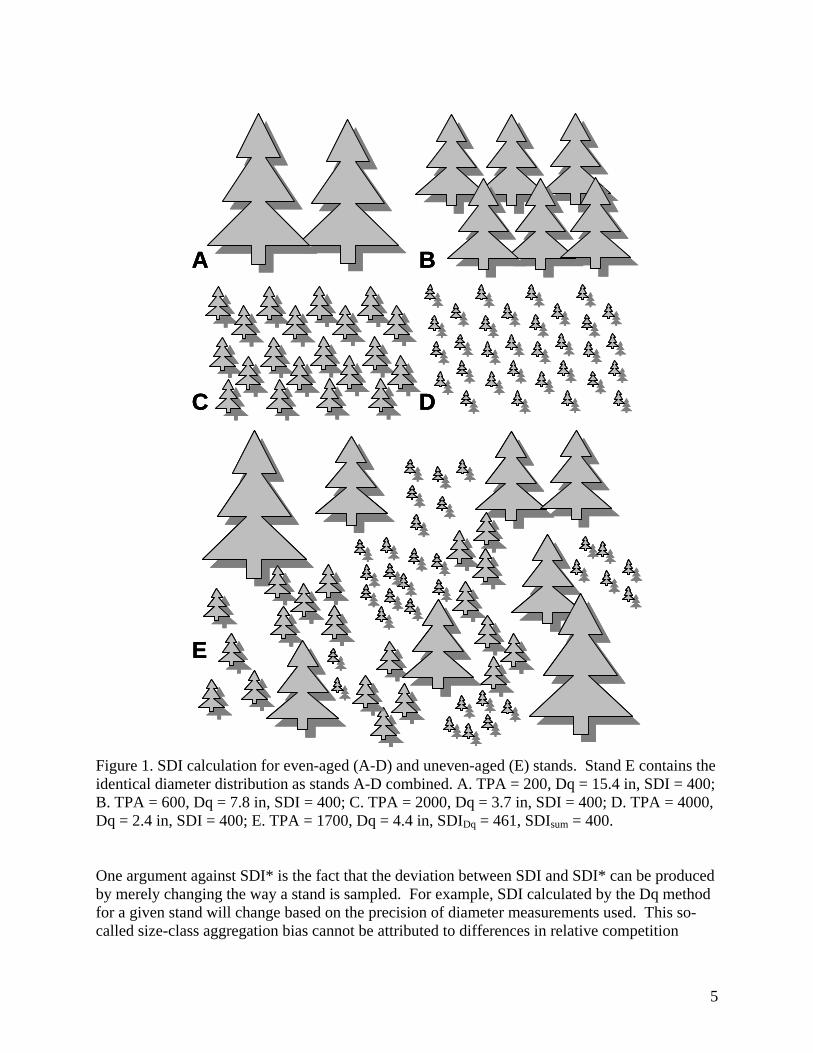
Figure 1. SDI calculation for even-aged (A-D) and uneven-aged (E) stands. Stand E contains the identical diameter distribution as stands A-D combined. A. TPA = 200, Dq = 15.4 in, SDI = 400; B. TPA = 600, Dq = 7.8 in, SDI = 400; C. TPA = 2000, Dq = 3.7 in, SDI = 400; D. TPA = 4000, Dq = 2.4 in, SDI = 400; E. TPA = 1700, Dq = 4.4 in, SDIDq = 461, SDIsum = 400. One argument against SDI* is the fact that the deviation between SDI and SDI* can be produced by merely changing the way a stand is sampled. For example, SDI calculated by the Dq method for a given stand will change based on the precision of diameter measurements used. This so-called size-class aggregation bias cannot be attributed to differences in relative competition

A

C D

B

E

A

C D

BA

C D

B

E

6

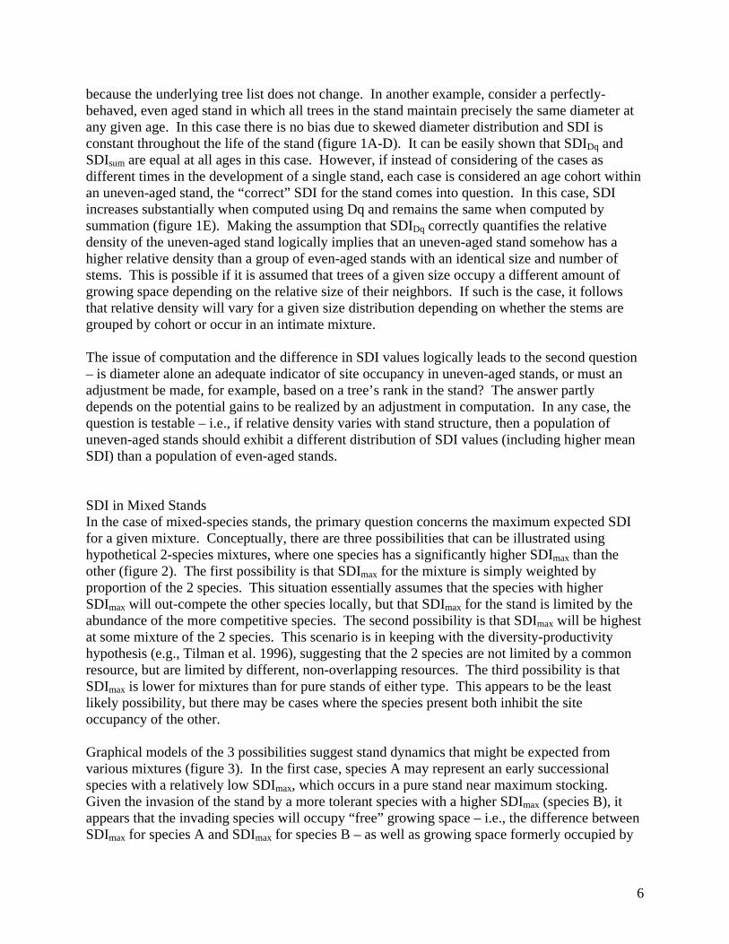
because the underlying tree list does not change. In another example, consider a perfectly-behaved, even aged stand in which all trees in the stand maintain precisely the same diameter at any given age. In this case there is no bias due to skewed diameter distribution and SDI is constant throughout the life of the stand (figure 1A-D). It can be easily shown that SDIDq and SDIsum are equal at all ages in this case. However, if instead of considering of the cases as different times in the development of a single stand, each case is considered an age cohort within an uneven-aged stand, the “correct” SDI for the stand comes into question. In this case, SDI increases substantially when computed using Dq and remains the same when computed by summation (figure 1E). Making the assumption that SDIDq correctly quantifies the relative density of the uneven-aged stand logically implies that an uneven-aged stand somehow has a higher relative density than a group of even-aged stands with an identical size and number of stems. This is possible if it is assumed that trees of a given size occupy a different amount of growing space depending on the relative size of their neighbors. If such is the case, it follows that relative density will vary for a given size distribution depending on whether the stems are grouped by cohort or occur in an intimate mixture. The issue of computation and the difference in SDI values logically leads to the second question – is diameter alone an adequate indicator of site occupancy in uneven-aged stands, or must an adjustment be made, for example, based on a tree’s rank in the stand? The answer partly depends on the potential gains to be realized by an adjustment in computation. In any case, the question is testable – i.e., if relative density varies with stand structure, then a population of uneven-aged stands should exhibit a different distribution of SDI values (including higher mean SDI) than a population of even-aged stands. SDI in Mixed Stands In the case of mixed-species stands, the primary question concerns the maximum expected SDI for a given mixture. Conceptually, there are three possibilities that can be illustrated using hypothetical 2-species mixtures, where one species has a significantly higher SDImax than the other (figure 2). The first possibility is that SDImax for the mixture is simply weighted by proportion of the 2 species. This situation essentially assumes that the species with higher SDImax will out-compete the other species locally, but that SDImax for the stand is limited by the abundance of the more competitive species. The second possibility is that SDImax will be highest at some mixture of the 2 species. This scenario is in keeping with the diversity-productivity hypothesis (e.g., Tilman et al. 1996), suggesting that the 2 species are not limited by a common resource, but are limited by different, non-overlapping resources. The third possibility is that SDImax is lower for mixtures than for pure stands of either type. This appears to be the least likely possibility, but there may be cases where the species present both inhibit the site occupancy of the other. Graphical models of the 3 possibilities suggest stand dynamics that might be expected from various mixtures (figure 3). In the first case, species A may represent an early successional species with a relatively low SDImax, which occurs in a pure stand near maximum stocking. Given the invasion of the stand by a more tolerant species with a higher SDImax (species B), it appears that the invading species will occupy “free” growing space – i.e., the difference between SDImax for species A and SDImax for species B – as well as growing space formerly occupied by

7

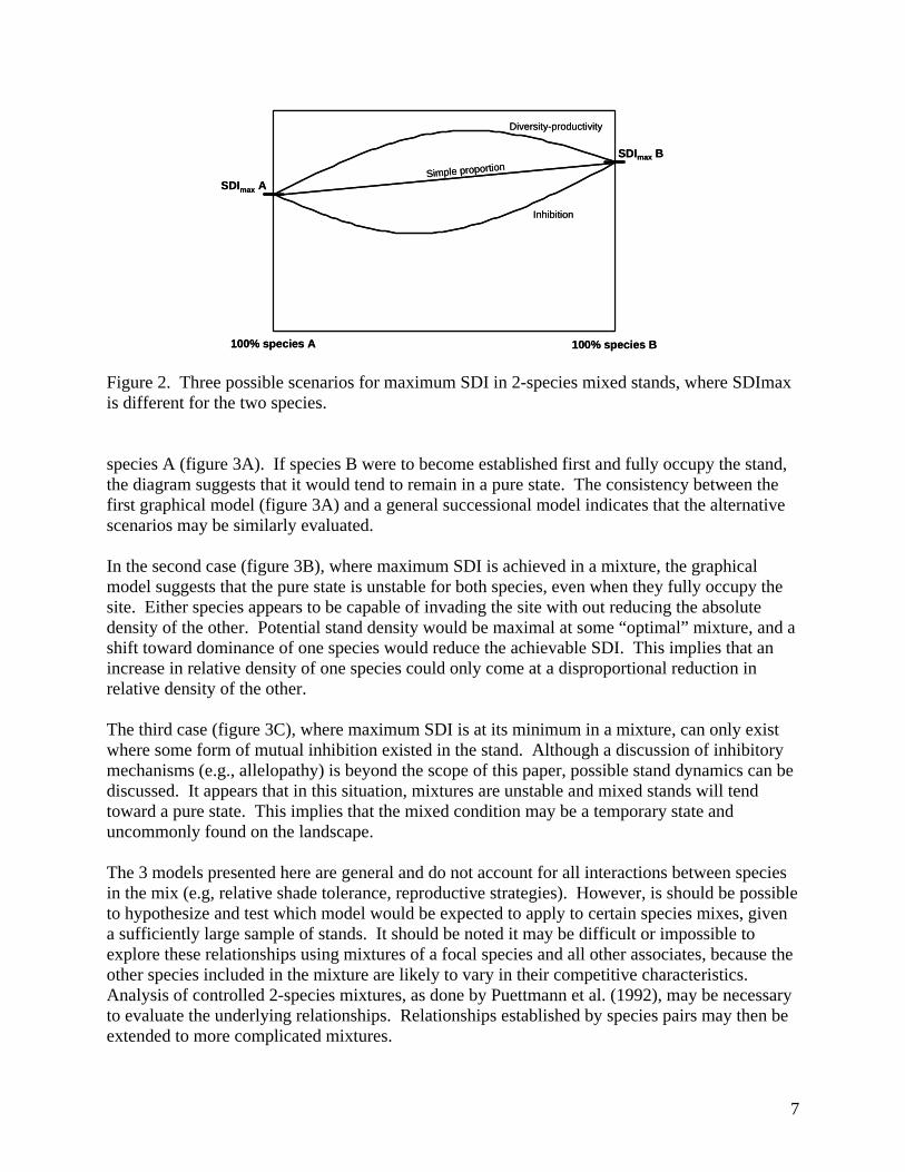
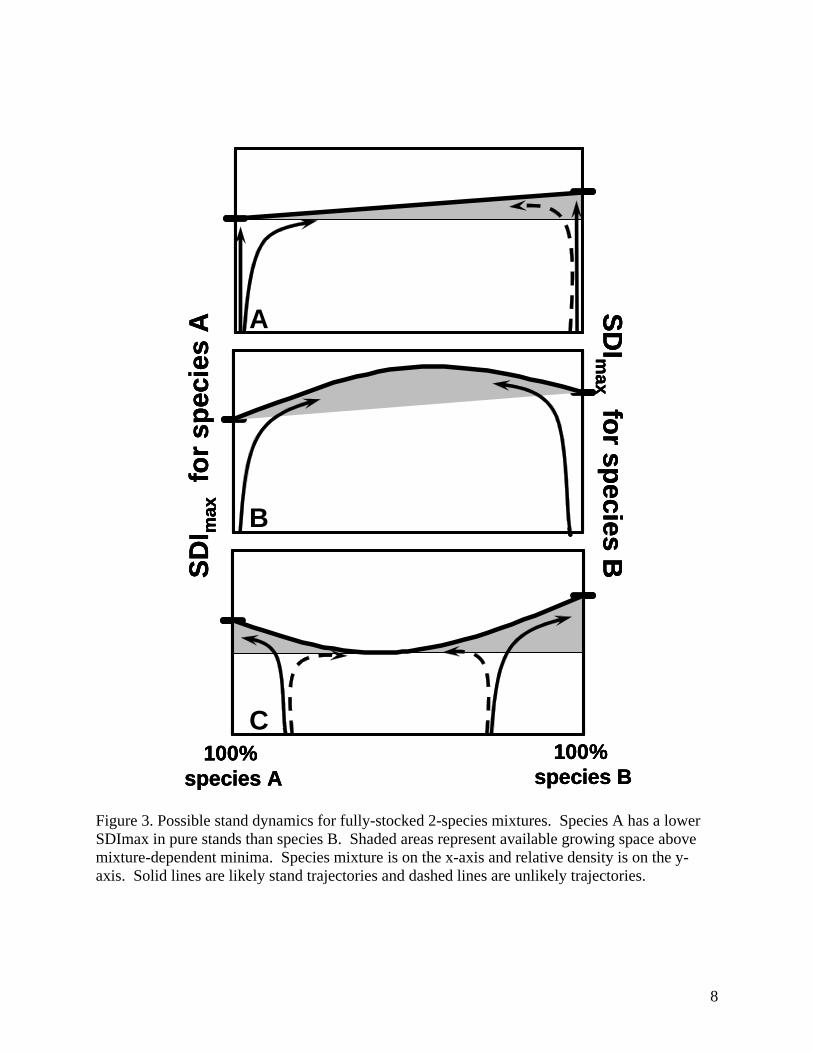
Figure 2. Three possible scenarios for maximum SDI in 2-species mixed stands, where SDImax is different for the two species. species A (figure 3A). If species B were to become established first and fully occupy the stand, the diagram suggests that it would tend to remain in a pure state. The consistency between the first graphical model (figure 3A) and a general successional model indicates that the alternative scenarios may be similarly evaluated. In the second case (figure 3B), where maximum SDI is achieved in a mixture, the graphical model suggests that the pure state is unstable for both species, even when they fully occupy the site. Either species appears to be capable of invading the site with out reducing the absolute density of the other. Potential stand density would be maximal at some “optimal” mixture, and a shift toward dominance of one species would reduce the achievable SDI. This implies that an increase in relative density of one species could only come at a disproportional reduction in relative density of the other. The third case (figure 3C), where maximum SDI is at its minimum in a mixture, can only exist where some form of mutual inhibition existed in the stand. Although a discussion of inhibitory mechanisms (e.g., allelopathy) is beyond the scope of this paper, possible stand dynamics can be discussed. It appears that in this situation, mixtures are unstable and mixed stands will tend toward a pure state. This implies that the mixed condition may be a temporary state and uncommonly found on the landscape. The 3 models presented here are general and do not account for all interactions between species in the mix (e.g, relative shade tolerance, reproductive strategies). However, is should be possible to hypothesize and test which model would be expected to apply to certain species mixes, given a sufficiently large sample of stands. It should be noted it may be difficult or impossible to explore these relationships using mixtures of a focal species and all other associates, because the other species included in the mixture are likely to vary in their competitive characteristics. Analysis of controlled 2-species mixtures, as done by Puettmann et al. (1992), may be necessary to evaluate the underlying relationships. Relationships established by species pairs may then be extended to more complicated mixtures.

100% species A 100% species B

SDImax B

SDImax A

Diversity-productivity

Simple proportion

Inhibition

100% species A 100% species B

SDImax B

SDImax A

Diversity-productivityDiversity-productivity

Simple proportionSimple proportion

InhibitionInhibition

8

Figure 3. Possible stand dynamics for fully-stocked 2-species mixtures. Species A has a lower SDImax in pure stands than species B. Shaded areas represent available growing space above mixture-dependent minima. Species mixture is on the x-axis and relative density is on the y-axis. Solid lines are likely stand trajectories and dashed lines are unlikely trajectories.

100% species A

100% species B

SDI m

axfo

r spe

cies

ASD

Imax

for species B

A

C

B

100% species A

100% species B

SDI m

axfo

r spe

cies

ASD

Imax

for species B

100% species A

100% species B

SDI m

axfo

r spe

cies

ASD

Imax

for species B

A

C

B

9

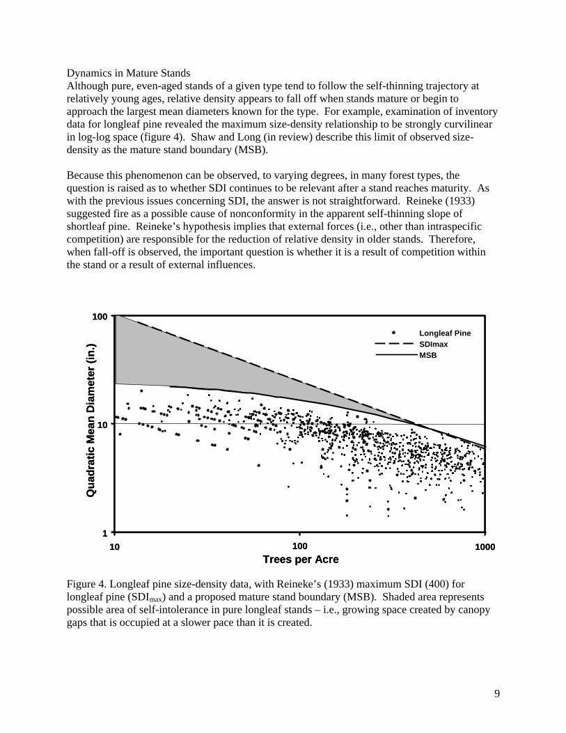
Dynamics in Mature Stands Although pure, even-aged stands of a given type tend to follow the self-thinning trajectory at relatively young ages, relative density appears to fall off when stands mature or begin to approach the largest mean diameters known for the type. For example, examination of inventory data for longleaf pine revealed the maximum size-density relationship to be strongly curvilinear in log-log space (figure 4). Shaw and Long (in review) describe this limit of observed size-density as the mature stand boundary (MSB). Because this phenomenon can be observed, to varying degrees, in many forest types, the question is raised as to whether SDI continues to be relevant after a stand reaches maturity. As with the previous issues concerning SDI, the answer is not straightforward. Reineke (1933) suggested fire as a possible cause of nonconformity in the apparent self-thinning slope of shortleaf pine. Reineke’s hypothesis implies that external forces (i.e., other than intraspecific competition) are responsible for the reduction of relative density in older stands. Therefore, when fall-off is observed, the important question is whether it is a result of competition within the stand or a result of external influences. Figure 4. Longleaf pine size-density data, with Reineke’s (1933) maximum SDI (400) for longleaf pine (SDImax) and a proposed mature stand boundary (MSB). Shaded area represents possible area of self-intolerance in pure longleaf stands – i.e., growing space created by canopy gaps that is occupied at a slower pace than it is created.

Trees per Acre

Qua

drat

ic M

ean

Dia

met

er (i

n.)

1

10

100

10 100 1000

Longleaf PineSDImaxMSB

Trees per Acre

Qua

drat

ic M

ean

Dia

met

er (i

n.)

1

10

100

10 100 1000

Longleaf PineSDImaxMSB

10

Zeide (2005) suggested that there are 2 causes of self-thinning: one caused by increase of stem diameter and the other caused by a decrease in self-tolerance. The former cause is the well-known mechanism of crowding, whereas the latter occurs when canopy gaps cannot be filled as fast as they are created. It is easy to visualize how fire, as well as insects, diseases, and other biotic and abiotic disturbances can lead to this situation. Zeide (2005) suggested that canopy gaps could be accounted for by extending the equation for SDI: [5] where e is the base of the natural logarithm, and b and c are parameters to be estimated. Although Zeide found that equation [5] explained variation in SDI only marginally over equation [2], the rate of re-occupancy of growing space created by canopy gaps is worth examining. In figure 4, there is an increasing gap between the mature stand boundary and SDImax with increasing Dq. The question is whether or not the zone of relative density represented by the gap is free growing space. As alternative to Zeide’s (2005) model, it is possible that the stand is still fully occupied at lower SDI values (i.e., self-thinning is the only mechanism in operation), but that SDI, which is based on stem diameter, does not adequately represent other factors that may be limiting in a mature stand (e.g., root competition). If this is the case, it follows that SDI, as a percentage of SDImax, is no longer representative of competition in the stand. Does this diminish the value of SDI an index? That question can only be answered by determining the nature of the gap in figure 4. If Zeide’s (2005) self-tolerance mechanism is in play, then it is expected that stand re-initiation would occur when relative density was sufficiently low as to allow regeneration of the dominant species. Establishment of more tolerant species may occur at higher relative densities, as discussed earlier. If the gap is not free growing space, but a reduction in SDI in an actively competing stand, then re-examination of SDI as a competition index is warranted. CONCLUSION It is apparent that the three issues that extend the concept of SDI are not completely independent. Stand dynamics and, consequently, site occupancy, are affected by structure and composition. The introduction of new species through succession and modification of composition by disturbances affects the potential maximum SDI. Also, differing analysis methods and data censorship approaches inevitably lead to differing results. Researchers must consider the relative effects of data characteristics and analysis methods on their results. Finally, it is worth noting that there is still interest in refining and extending Reineke’s SDI 72 years after it was introduced, and the level of interest may be at its highest ever. One explanation for the level of interest is that SDI is an application-oriented measure, and practitioners are constantly in search of the “better mousetrap.” Therefore work continues on extensions to the concept, as well as analysis of SDI for lesser-studied species and forest types.

( )10

10−⎟

⎠⎞

⎜⎝⎛= Dqc

b

eDqTPASDI

11

LITERATURE CITED ANDO, T., 1962. Growth analysis on the natural stands of Japanese red pine (Pinus densiflora Sieb. et Zucc.). II. Analysis of stand density and growth. Bulletin of the Government Forest Experiment Station 147: 71–77. ANDO, T. 1968. Ecological studies on the stand density control in even-aged pure stand. Tokyo Government Forest Experiment Station Bulletin 210:1-153. BAKER, F.S. 1934. Theory and practice of silviculture. New York: McGraw-Hill, 502 p. BI, H. 2001. The self-thinning surface. Forest Science 47:361-370. BI, H., and N.D. TURVEY. 1997. A method of selecting data points for fitting the maximum density-biomass line for stands undergoing self-thinning. Australian Journal of Ecology 22:356-359. BI, H., G. WAN, and N.D. TURVEY. 2000. Estimating the self-thinning boundary line as a density-dependent stochastic biomass frontier. Ecology 81:1477-1483. BRUCE, D., and F.X. SCHUMACHER. 1942. Forest mensuration. New York: McGraw-Hill, 425 p. DANIEL, T.W., R.L. MEYN, and R.R. MOORE. 1979. Reineke’s stand density index in tabular form in English and metric units with its applications. Utah Agricultural Experiment Station, Research Report 37. Logan, Utah. DREW, T.J., and J.W. FLEWELLING. 1977. Some recent Japanese theories of yield-density relationships and their application to Monterey pine plantations. Forest Science 23:517-534. DREW, T.J., and J.W. FLEWELLING. 1979. Stand density management: an alternative approach and its application to Douglas-fir plantations. Forest Science 25:518-532. DUCEY M.J., and B.C. LARSON. 2003. Is there a correct stand density index? an alternate interpretation. Western Journal of Applied Forestry 18:179-184. JACK, S.B., and J.N. LONG. 1996. Linkages between silviculture and ecology: an analysis of density management diagrams. Forest Ecology and Management 86:205-220. KIRA, T., H. OGAWA, and N. SAKAZAKI. 1953. Intraspecific competition among higher plants, I. Competition-yield-density interrelationship in regularly dispersed populations. Journal of the Institute of Polytechnics, Osaka City University, Series D:1–16. MEYER, H.A. 1953. Forest mensuration. State College, PA: Penns Valley Publishers, 357 p.

12

LEDUC, D.J. 1987. A comparative analysis of the reduced major axis technique of fitting lines to bivariate data. Canadian Journal of Forest Research 17:654-659. LONG, J.N., and T.W. DANIEL. 1990. Assessment of growing stock in uneven-aged stands. Western Journal of Applied Forestry 5:93-96. LONG, J.N., and J.D. SHAW. 2005. A density management diagram for even-aged ponderosa pine stands. Western Journal of Applied Forestry 20:205-215. NEWTON, P.F. 1997. Stand density management diagrams: Review of their development and utility in stand-level management planning. Forest Ecology and Management 98:251–265. OSAWA, A., and S. SUGITA. 1989. The self-thinning rule: another interpretation of Weller’s results. Ecology 70:279-283. PUETTMANN, K.J., D.E. HIBBS, and D.W. HANN. 1992. The dynamics of mixed stands of Alnus rubra and Pseudotsuga menziesii: extension of size-density analysis to species mixture. Journal of Ecology 80:449-458. PRETZSCH, H., and P. BIBER. 2005. A re-evaluation of Reineke’s rule and stand density index. Forest Science 51:304-320. REINEKE, L.H. 1933. Perfecting a stand-density index for even-aged forests. Journal of Agricultural Research 46:627-638. SACKVILLE HAMILTON, N.R., C. MATTHEW, and G. LEMAIRE. 1995. In defence of the -3/2 boundary rule: a re-evaluation of self-thinning concepts and status. Annals of Botany 76:569-577. SAUNDERS, M.R., and K.J. PUETTMANN. 2000. A preliminary white spruce density management diagram for the Lake States. University of Minnesota, Department of Forest Resources Staff Paper Series No. 145 SHAW, J.D. 2000. Application of stand density index to irregularly structured stands. Western Journal of Applied Forestry 15:40-42. SHAW, J.D., and J.N. LONG. In review. A density management diagram for longleaf pine stands. Southern Journal of Applied Forestry. SHINOZAKI, K., and T. KIRA. 1956. Intraspecific competition among higher plants. VII. Logistic theory of the C-D effect. Journal of the Institute of Polytechnics, Osaka City University, Series D 7:35-72. STAGE, A.R. 1968. A tree-by-tree measure of site utilization for grand fir related to stand density index. USDA Forest Service Research Note INT-77. Intermountain Forest and Range Experiment Station, Ogden, UT.

13

TILMAN, D., D. WEDIN, and J. KNOPS. 1996. Productivity and sustainability influenced by biodiversity in grassland ecosystems. Nature 379:718-720. VACCHIANO, G., E. LINGUA, and R. MOTTA. 2005. Valutazione dello Stand Density Index in popolamenti di abete rosso (Abies alba Mill.) nel Piemonte meridionale [Evaluation of Stand Density Index in southern Piedmont silver fir (Abies alba Mill.) stands]. L’Italia Forestale e Montana 3:269-286. WELLER, D.E. 1987. A reevaluation of the -3/2 power rule of plant self-thinning. Ecological Monographs 57:23-43. WELLER, D.E. 1990. Will the real self-thinning rule please stand up? – a reply to Osawa and Sugita. Ecology 71:1204-1207. YODA, K., T. KIRA, H. OGAWA, and K. HOZUMI. 1963. Intraspecific competition among higher plants. XI. Self-thinning in overcrowded pure stands under cultivated and natural conditions. Journal of the Institute of Polytechnics, Osaka City University, Series D. 14:107-129. ZEIDE, B. 1983. The mean diameter for stand density index. Canadian Journal of Forest Research 13:1023-1024. ZEIDE, B. 2005. How to measure stand density. Trees 19:1-14.