This paper presents preliminary findings and is being distributed to economists

and other interested readers solely to stimulate discussion and elicit comments.

The views expressed in this paper are those of the authors and do not necessarily

reflect the position of the Federal Reserve Bank of New York or the Federal

Reserve System. Any errors or omissions are the responsibility of the authors.

Federal Reserve Bank of New York

Staff Reports

Regulatory Changes and

the Cost of Capital for Banks

Anna Kovner

Peter Van Tassel

Staff Report No. 854

June 2018

Revised October 2018

Regulatory Changes and the Cost of Capital for Banks

Anna Kovner and Peter Van Tassel

Federal Reserve Bank of New York Staff Reports, no. 854

June 2018; revised October 2018

JEL classification: G12, G21, G28

Abstract

We estimate the cost of capital for the banking industry and find that, while the cost of capital

soared for banks during the financial crisis, after the passage of the Dodd–Frank Act, the value-

weighted cost of capital fell differentially more for banks than for nonbanks. The very largest

banks drive the decline in expected returns, with some evidence indicating that stress testing has

lowered the cost of capital for the very largest stress-tested banks. Changes to banks’ cost of

capital have real economic consequences—we find that increases in banks’ cost of capital are

associated with tightening in credit supply.

Key words: cost of capital, beta, bank regulation, Dodd-Frank Act, banks

_________________

Kovner, Van Tassel: Federal Reserve Bank of New York (emails: anna.kovner@ny.frb.org, peter.vantassel@ny.frb.org). The authors are grateful to Charles Calomiris, Mark Carey, Douglas Diamond, Fernando Duarte, George Pennacchi, René Stulz, Jeffrey Wurgler and seminar participants at Chicago Booth, the NBER Risks of Financial Institutions conference, and the Federal Reserve Bank of New York’s Effects of Post-Crisis Banking Reforms conference for comments. They also thank Davy Perlman, Anna Sanfilippo, and Brandon Zborowski for outstanding research assistance. Any errors or omissions are the responsibility of the authors. The views expressed in this paper are those of the authors and do not necessarily reflect the position of the Federal Reserve Bank of New York or the Federal Reserve System.

To view the authors’ disclosure statements, visit https://www.newyorkfed.org/research/staff_reports/sr854.html.

1 Introduction

The cost of capital reflects the perceived risk of a company’s equity to investors. Managersseek to earn or outperform their cost of capital. For banks, the cost of capital drives lendingamounts, borrowing rates, and thus real economic activity.1 But what is the cost of capitalfor banks and how has it changed with regulation? In this paper we calculate the cost ofcapital for banks over the last twenty years and link this cost to survey measures of banklending supply.

We find that, in net, regulations following the financial crisis have significantly lowered thecost of capital for banks relative to the all-time highs experienced during the crisis. Lookingover a longer horizon and accounting for changes in the risk-free rate, banks’ cost of capitalappears to have reverted to levels higher than those experienced before the deregulation ofthe 2000s. However, our estimates of the difference between the post-Dodd-Frank period andthe pre-Gramm-Leach-Bliley period depends on the cost of capital measure and specification.By some measures, the cost of capital is lower today or the difference cannot be statisticallydistinguished from zero. Changes to the cost of capital matter – we find that changes to ourcost of capital estimates are associated with changes in bank credit supply and loan spreads.

One contribution of this paper is to understand the effects of regulation on banks throughthe lens of stock prices. We do this by comparing changes in the cost of capital for banksand non-banks, separating the last twenty years by key dates in bank regulation includingthe: Gramm-Leach-Bliley Act (November 1999), Financial Crisis (January 2007), Supervi-sory Capital Assessment Program (May 2009), and Dodd-Frank Act (July 2010). Since thepassage of the Dodd-Frank Act (DFA), the value-weighted cost of capital has averaged 11%for banks and 8% for non-banks.2 For all firms, including banks, average levels of expectedreturns on equity and weighted average costs of capital are much lower than the levels fromthe late 1990s, primarily reflecting the 4.5% decline in the risk-free rate.

In order to separate the effects of regulation from market wide changes in expectedreturns, we compare the change in the cost of capital for banks to the change in that of non-banks over time. This difference-in-differences approach allows us to distinguish betweendifferences in expected returns for investors that affect all companies, such as changes to therisk-free rate and to risk premia, and differences in regulation that affect only banks. Forbanks, cost of capital estimates spiked in the period following the financial crisis, averaging

1Cummins et al. (1994), Philippon (2009), Gilchrist et al. (2013), and Brunnermeier and Sannikov (2014).2Throughout the paper we refer to expected equity returns as the cost of capital, although we we also

explore other cost of capital metrics such as the weighted average cost of capital (WACC). Mechanically, thevalue-weighted sum of bank and non-bank stock returns is the aggregate stock market return whose cost ofcapital is equal to the risk-free rate plus the equity risk premium.

1

more than 15% on a value-weighted basis. The cost of capital did not increase by nearlyas much for non-banks. Comparing the period following the passage of the DFA to theimmediate prior time period, the cost of capital fell by approximately 4.5% more for banksrelative to non-banks, a difference that is economically and statistically significant and robustto different approaches for estimating the cost of capital. When comparing the post Dodd-Frank period to the period before the passage of the Gramm-Leach-Bliley Act (GLB) in 1999,which repealed provisions from the Glass-Steagall Act of 1933 that separated investmentbanking and commercial banking activities, the cost of capital for non-banks has fallen by1% to 2%. However, this result is not robust across specifications or cost of capital measures,with some of our cost of capital measures reaching the opposite conclusion. Taken together,these results suggest that post-crisis bank regulation reduced expected returns from post-crisis highs, but that the cost of capital for banks may be higher than it was twenty yearsago.

To confirm that we are capturing regulation, we do several additional analyses. In par-ticular, the cost of capital for banks may change relative to non-banks for reasons other thanregulation. For example, if investors revalue the riskiness of bank assets at the same timethat regulations are changing, we may spuriously attribute the changes in asset betas toregulation. We account for this observation by taking three approaches. First, we comparebanks to only non-bank financial intermediaries, a control group of firms that has assetsand business models that are more closely related to that of banks but that is not directlyaffected by changes to bank regulation. We find similar results from this comparison – thecost of capital falls by more for banks than for non-bank financials after DFA, and remainshigher than that of non-bank financials when comparing the current time period to the late1990s. Second, since banks may respond differently to changes in interest rates, we confirmthat our results are robust to controlling for the level of interest rates and the term spreadwhen modeling stock returns.

Third, since many recent financial regulatory reforms apply only to the largest banks,we ask if changes in the cost of capital for the very largest banks relative to smaller banksare different from changes in the cost of capital for the very largest non-banks relative tosmaller firms in the same industries. This analysis is particularly relevant when estimatingchanges around the passage of the DFA, as several DFA provisions specifically target thelargest banks. We find that large banks are different from small banks on average, with acost of capital that is 3% higher from 1996 to 2017. Large banks also drive the differentialchanges in the cost of capital relative to non-banks, with the very largest banks exhibitingboth the largest increase in their cost of capital after the financial crisis as well as the largestdecrease after DFA. Over a longer horizon that compares the current period to the pre-GLB

2

period, the cost of capital for the largest non-banks relative to smaller non-banks has fallenby around 2%. The difference for the largest banks relative to smaller banks has changedby even more, exhibiting an additional decline of 1% to 2% that is is significant in severalspecifications.

In the last two decades, the cost of capital fell the most for banks and non-bank financialintermediaries relative to other firms after the passage of the Gramm-Leach-Bliley Act.This result highlights the importance of the comparison period and the comparison set ofcompanies when measuring changes in the cost of capital. For example, Sarin and Summers(2016) compare a pre-crisis period from 2002-2007 to a post-crisis period from 2010-2015and find that the cost of capital has increased for banks. Their conclusions are driven, inpart, by the fact that the comparison period from 2002-2007 is a time that coincides withunusually low expected returns for banks. However, this also points to some limitations ofinterpreting the aggregate cost of capital for banks as a measure of systemic risk that wouldbe important to policy makers – the exact years in which cost of capital estimates for bankswere unusually low were exactly the years in which ex-post realizations suggest that tail riskwas growing in the banking industry. At the same time, cross-sectional differences in bankbetas may still reflect differences in systematic risk across banks. In the opposite directionto understanding changes over time, pooling all time periods can also affect conclusions.Minton et al. (2017) pool data over a long horizon and find that differences between thecost of capital for large and small banks are fully captured by the Fama and French (1993)three-factor model. In contrast, we see differential changes in expected returns for the twentylargest banks when we split the time periods up by significant dates in bank regulation. Tothe extent that the value of government guarantees are falling during this time period, assuggested by Atkeson et al. (2018), the decrease in systemic risk stemming from the DFAmay be even more dramatic than decline implied by the cost of capital analysis, as declininggovernment guarantees would tend to push the cost of capital for the largest banks higher.

What drives these changes in the cost of capital for banks? From an asset pricing per-spective, the cost of capital is determined by a firm’s exposures, or betas, to systematic risk,as well as the price of systematic risk as perceived by investors. Narrowing our analysis tothe set of bank holding companies and banks for which we have regulatory data, we explorehow much of the change in the cost of capital is associated with changes in banks’ assetmix, leverage, and liquidity. In value-weighted regressions, we find that unconditional con-trols have little impact on the results, indicating that changing bank characteristics do notexplain changes in the cost of capital within banks over time. However, when we allow fortime-varying relationships between bank characteristics and the cost of capital, consistentwith the spirit of Calomiris and Nissim (2014) and Minton et al. (2017), we do find that some

3

characteristics are valued differently over time. The association between risk weighted assets(RWA) and expected returns peaks in the aftermath of the financial crisis. A one standarddeviation increase in RWA results in a 1% change in the cost of capital in the period followingthe financial crisis, but this association falls again after the Dodd-Frank Act. This appearsto be driven by changes in expected returns for loans and loan commitments, particularlyreal estate loans. It is this change in the market price of the systematic risk of RWA thatexplains most of the post financial crisis fall in expected returns for banks.

A key contribution of our paper is to link these changes in the cost of capital to measuresof the quantity and pricing of loan supply. We establish this link by making use of confidentialmicro survey response data from the Senior Loan Officer Opinion Survey (SLOOS), a surveycommonly used to measure banks’ willingness to lend. We find that changes in the cost ofcapital are associated with changes in both the supply and the pricing of credit. This resultholds both in aggregate for the panel of surveyed banks as well as in the cross section aftercontrolling for business cycle variation - when banks’ cost of capital increases, banks tightenloan standards and increase loan spreads. Through this channel, changes in regulation thatimpact banks’ cost of capital are passed through to the real economy.

We estimate our baseline cost of capital measures using the CAPM because it is a bench-mark single-factor equilibrium model that is easy to interpret. The CAPM cost of capitalis also an important metric because confidential supervisory work, survey evidence (Gra-ham and Harvey 2001), and the revealed preferences of investors (Berk and van Binsbergen2016) indicate that it is favored by practitioners, and therefore impacts corporate and invest-ment decision making. However, we also provide a range of robustness checks and analysisfor additional cost of capital measures including three-factor estimates (Fama and French1993), five-factor estimates that incorporate additional interest rate and term spread factors,weighted average cost of capital estimates, one-factor estimates with a time-varying equityrisk premium, log CAPM betas, and asset betas estimated from the Merton (1974) model.We highlight in the text when these measures coincide and differ from our baseline CAPMcost of capital estimates. Across the various estimates of expected equity returns, we consis-tently find a significant decrease in the cost of capital for the largest banks since the passageof the DFA.

The paper proceeds as follows. Section 2 presents a review of the literature on the costof capital and the use of market measures to estimate the effects of changes to regulation.Sections 3 and 4describe our approach to calculating the cost of capital and our difference-in-difference empirical approach to understand the changes in the time series of the costof capital for banks. Section 5 discusses the results for the baseline CAPM cost of capitalestimates. Section 6 presents evidence that the cost of capital matters, by demonstrating

4

the association between the cost of capital and banks’ supply of loans. Section 7 providesrobustness checks using alternative cost of capital measures. The paper concludes with asummary of our findings as well as a discussion of the limitations of the approach.

2 Literature review

There is a long literature devoted to estimating the cost of capital for firms. Empiricalstudies often exclude the banking industry due to differences in accounting ratios such asleverage between banks and non-financial firms. One of the first papers to look at financialfirms was Barber and Lyon (1997) who sought a sample not used in the original identifi-cation of the three-factor Fama and French (1993) model. Barber and Lyon (1997) findsimilar relationships between size, book-to-market and stock returns for financial firms andnon-financial firms. Schuermann and Stiroh (2006) look at a sample of bank stock returnsfrom 1997 to 2005, adding bank specific factors such as such as interest rate and credit vari-ables. Their conclusions for banks are twofold – first, the market factor (RMRF) dominates,followed closely by the size (SMB) and value (HML) factors from Fama and French (1993).They do not find significant explanatory power from rate and credit factors. Second, theyfind evidence of correlated residuals, suggesting the possible presence of additional factorsthat price bank equity returns. Adrian et al. (2016) identify two additional factors thataccount for much of these correlated residuals – financial sector return on equity (FROE)and the spread between financials and the market (SPREAD). Gandhi and Lustig (2015)study differences in returns of large and small banks, identifying a size-dependent factorthat they hypothesize captures tail risk. They study the reaction of this factor to regulatorychanges, such as the Gramm-Leach-Bliley roll-back of the Glass-Steagall Act, and find thatthe implied subsidy to banks increases when regulations are relaxed. Related to this finding,King (2009) documents a fall in the CAPM cost of capital for 89 global banks in the early2000s. Baker and Wurgler (2015) demonstrate that the low risk anomaly holds within thecross-section of bank stocks, centering their analysis on CAPM. Banks with low (high) betasearn higher (lower) returns than predicted by the CAPM. As a result, their study highlightsthe weak relationship between cost of capital estimates from the CAPM and the realizedreturns of bank stocks.

This literature motivates our estimation of the Fama and French (1993) three-factor (FF3)model as a robustness check for the CAPM analysis. While there are alternative multi-factormodels that provide superior in-sample fit relative to the CAPM and FF3 models, we arereluctant to use these larger models for our baseline analysis, although we do report results fora five-factor model that combines the FF3 factors with interest rate and term spread factors

5

as a robustness check due to the importance of interest rates for banks. The more the factorsdiverge from a micro-founded asset pricing model, the harder they may be to interpret fromthe perspective of a manager looking to estimate a discount rate for the systemic risk of thecash flows for a marginal project. In addition, other studies such as Linnainmaa and Roberts(2016) criticize multi-factor models for poor out-of-sample performance and data snooping.

Another strand of the literature relates changes in regulation to market measures. Thesepapers often focus on Tobin’s q, but sometimes include measures of the cost of equity as well.Minton et al. (2017) find that Tobin’s q is lower for large banks than for small banks anddecreases with asset size when a bank exceeds the Dodd-Frank threshold. They estimate thecost of capital for banks from 1987 to 2006 using both three and five-factor models and arguethat after including the size factor, the price of risk for the largest banks (greater than $50billion) is similar to that of smaller banks. Similarly, Calomiris and Nissim (2014) explorethe relationship between market-to-book and bank characteristics after the crisis. Theyattribute changes in valuations after the crisis to a decline in the value of intangibles ratherthan changing regulations, including changes in intangible loan and deposit relationships,market valuation of non-interest income and steepness of the yield curve. Huizinga andLaeven (2012) examine how Tobin’s q relates to the composition of assets of large banks,finding that lower levels of market-to-book after the financial crisis reflect asset re-valuations,particularly for real estate loans at larger banks. While many papers focus on a singlemeasure, including our analysis of the cost of capital, Sarin and Summers (2016) comparevarious market-based measures of risk before and after the crisis (2002-2007 vs. 2010-2015)for the largest domestic and international banks. Comparing those time periods, they findflat or higher levels of volatility, beta, and risk for the largest banks in the post-crisis period.Sarin and Summers (2016) also document lower market-to-book ratios for banks in the post-crisis period, which they attribute to lower bank profitability or franchise value. Atkesonet al. (2018) investigate this result and suggest a method for decomposing market-to-bookratios into franchise value and government guarantee components, finding that both franchisevalues and, even more so, government guarantees have declined in the post-crisis period.

We add to this literature a comprehensive empirical study comparing the prevailingmethods of calculating the cost of capital and identifying ways in which these measuresoffer similar or different implications for changes in the cost of capital for banks since 1996.Rather than proposing a new method or additional factor, we think about the implicationsfor bank managers of the different measures and how measure choice might have differentimplications. This analysis also contributes to the literature that relates the cost of capital toinvestment. For non-financials, Philippon (2009) and Gilchrist and Zakrajšek (2012) studythe relationship between the cost of debt and firm level investment. Frank and Shen (2016)

6

extend this work to include weighted average cost of capital and cost of equity measures.These papers find that the cost of debt and the weighted average cost of capital matterfor investment, but that the weighted average cost of capital results are sensitive to theestimation approach for computing the cost of equity. In comparison to these results fornon-financial firms and investment, we believe our study is the first to directly relate thecost of capital for banks to bank lending supply, identified at the bank level rather than inaggregate or in portfolios.

3 Estimating the cost of capital

The cost of capital depends on the expected return of equity investors as well as the timevalue of money as captured by the risk-free rate. Empirically, expected stock returns are notobservable. Instead, we must rely on economic or statistical models to estimate expectedreturns. As a result, any test regarding the cost of capital is a joint test of the null hypothesisand the model that is used to estimate expected returns (Fama 1970, 1991). Most of ouranalysis focuses on the cost of equity, which is often emphasized in the banking industry.However, in Section 7.3, we also analyze the weighted average cost of capital, which incor-porates measures of the cost of debt and deposits that comprise the vast majority of bankfunding.

A key challenge when measuring the cost of capital is stock market volatility. Excessvolatility creates a large noise to signal ratio that makes estimating expected returns difficult.To see this, note that even with a constant risk premium and log-normal returns, it wouldstill take over 40 years to estimate the risk premium, or expected return, with a standarderror of 3% when annualized volatility is 20% (Merton 1980). Empirically, this example turnsout to be quite accurate. From 1978 to 2017, the average market risk premium has been8% with a standard error of 2.5%.3 The resulting confidence interval from subtracting andadding 1.96 standard errors ranges from 3.1% to 12.9%, almost 10% wide. In multi-factorsettings such as the ICAPM of Merton (1973) or the APT of Ross (1976), the correspondinguncertainty in factor risk premiums, or factor expected returns, dominates the imprecisionin estimating expected stock returns. As Fama and French (1997) put it, “our message isthat uncertainty of this magnitude about risk premiums, coupled with the uncertainty aboutrisk loadings, implies woefully imprecise estimates of the cost of equity.”

In contrast to expected returns, time-varying volatilities and covariances can be estimated

3The market risk premium is estimated by regressing CRSP value-weighted returns in excess of the one-month Treasury bill rate onto a constant. Monthly returns are multiplied by 12 to compute an annualizedestimate. The Newey-West standard error is 2.49% using 5 lags and the White standard error is 2.41%.

7

with precision using high frequency data (Merton 1980). As a result, the contribution of theuncertainty in betas, or factor risk loadings, to cost of capital estimates is relatively smallcompared to the uncertainty in expected returns, or factor risk premiums. An implicationof this result is that changes in betas can plausibly identify changes in the cost of capital.In particular, if the CAPM of Sharpe (1964) and Lintner (1965) holds and the market riskpremium is roughly constant over the period of interest, we can use time variation in preciselyestimated betas to document how the cost of capital is changing for banks relative to otherfirms, even if there is large uncertainty surrounding the level of the cost of capital itself.However, if the true model is a multi-factor model or the market risk premium is time-varying, analysis based on the CAPM assuming a constant risk premium may be biased.

With these limitations in mind, we estimate our baseline cost of capital measures usingthe CAPM assuming a constant market risk premium. We define our baseline cost of capitalestimates for the CAPM as,

Et[Ri,t+1] = Rf,t + βi,t · µ. (1)

The first term is the risk-free rate Rf,t. The second term is a time-varying CAPM beta βi,t.The last term is the equity risk premium µ, which we assume is constant. We set the risk-freerate to the three-month Treasury bill rate and the equity risk premium to 8%, the averageCRSP value-weighted excess return from 1926 to 2017. The betas are estimated from one-year rolling regressions of firm level daily excess returns onto market excess returns. Themarket return is the CRSP value-weighted return obtained from Ken French’s website. Theestimates are ex-ante betas in the sense that each month the beta is computed using laggeddaily data over the previous 252 trading days.

As the discussion makes clear, a number of alternative choices can be made when esti-mating the cost of capital. We have focused on factor models that rely on three components:the risk-free rate, the factor loadings, and the factor risk premiums. There are multipleways to estimate each of these components. For example, one could estimate the risk-freerate with the one-month Treasury bill or overnight index swaps instead of the three-monthTreasury bill. This choice has a minor impact on the level of the cost of capital that af-fects all firms equally. In most of the specifications, we will subtract the risk-free rate fromthe cost of capital estimates to make the differences-in-differences even easier to interpret.4

Other choices such as the method for estimating the factor loadings and risk premiums havea larger impact. For example, to name a few methods from a large literature, betas can beestimated from five year rolling regressions with monthly data, one year rolling regressions

4Since we have an unbalanced panel, changes in the number of firms over time will allow the level of therisk-free rate to potentially impact the estimated difference-in-difference coefficients in the panel regressionswhen the dependent variable is the expected return rather than the excess expected return.

8

with daily data, and directly from estimates of firm level volatility and firm level correlationwith the market.5 Betas may also use lagged, centered, or forward data depending on theapplication. Given our interest in how the cost of capital has varied over time, we preferusing daily data (252 observations per year) to deliver more precise and less biased estimatesin comparison to slow moving estimates from monthly data (60 observations per five years).

Finally, one must decide how to estimate the factor risk premiums. We do this by usingthe simple time-series average of tradeable factor excess returns. An alternative approach isto allow for time-varying factor risk premiums from return predictability regressions, equilib-rium models, or dividend discount models (Duarte and Rosa 2015). While there is ample em-pirical evidence that risk premia do vary over time (Cochrane 2011), estimating time-varyingrisk premia is challenging due to the aforementioned difficulties in estimating expected stockreturns. Welch and Goyal (2007) find that many estimates of the equity risk premium areunstable out of sample, underperforming the historical mean model that we use in this paper.An implication of our approach is that we rely on time-series and cross-sectional differencesin betas to identify changes in the cost of capital over time. As a robustness check, we alsopresent results from a one-factor model with a time-varying equity risk premium.

4 Changes over time in the cost of capital

Changes in expected returns for the banking industry over time are shown in Figure 1,which shows the monthly value-weighted average cost of capital for banks, with horizontallines at the means of the different regulatory time periods. By calculating these averages ina time series panel regression format instead of looking at simple averages, we can control fordifferences in the composition of the panel and for firm characteristics while adjusting thestandard errors to account for the fact that the observations are not independent (neitherover time nor within firm). This allows us to construct confidence intervals around our timeperiod measures while also investigating differences-in-differences specifications that comparechanges in estimated expected returns for all the non-bank firms in the CRSP database tochanges in expected returns of banks.

4.1 Regulatory time periods

We compare changes in the cost of capital across time periods in which bank regulationschanged from 1996 to 2017. The periods are:

5For example, see Scholes and Williams (1977), Fama and French (1997), Lewellen and Nagel (2006),Ang and Kristensen (2012), Frazzini and Pedersen (2014), Baker and Wurgler (2015), and Adrian et al.(2016).

9

1. Basel I: Pre-period (March 1996 to October 1999)

2. GLB: The Gramm-Leach-Bliley Act (November 1999 to December 2006)

3. Crisis: The Financial Crisis (January 2007 to April 2009)

4. SCAP: The Supervisory Capital Assessment Program (May 2009 to June 2010)

5. Dodd-Frank: The Dodd-Frank Act (July 2010 to December 2017)

We define break points as the month of the passage of the relevant banking law. Resultsare similar if we vary the time periods within a few months to capture anticipation of thepassage of the law. To see how the cost of capital has changed over time, we begin ouranalysis by estimating the following specification:

Et[Ri,t+1] = α+ β1GLBt + β2Crisist + β3SCAPt + β4Dodd-Frankt + ei,t (2)

where GLBt, Crisist, SCAPt, and Dodd-Frankt are binary variables equal to one duringthe periods defined above. The omitted pre-period begins twenty years ago in 1996 and thusis characterized by the Basel I regulatory regime.

The estimated coefficient for each time period is the difference between the average costof capital in that time period relative to the pre-period, whose value is captured by theconstant term. The null hypothesis is that all β are equal to 0 – meaning that there have notbeen any changes to expected returns over time and that as a result, regulatory changes havenot changed the cost of capital. We estimate the specifications both on a value-weightedbasis, which gives us an understanding of changes for the industry in aggregate, as well as onan equal-weighted basis, which places equal value on each company in the panel. Standarderrors are clustered by firm and by month. Results are similar if the analysis incorporatesearlier data (back through 1986), however, we focus on the more recent time period to haveconsistency in the regulatory data, which becomes available for all fields used in the analysisin 1996:Q1.

4.2 Sample selection and definition of banks

We use CRSP, Compustat, and regulatory data from call reports and Y-9C filings fromMarch 1996 to December 2017 for our baseline analysis. We estimate the cost of capital forall CRSP firms with share codes 10 or 11 that are traded on the NYSE, NASDAQ, or AMEX.Later in the paper we also estimate the weighted average cost of capital (WACC) by mergingquarterly Compustat data onto monthly CRSP data using the most recent observation that

10

was announced prior to the start of the month (based on RDQ date). We filter observationsfrom this dataset with missing cost of capital estimates or missing Compustat asset data aswell as observations with share prices that are less than one dollar. The resulting sampleincludes a panel of 1,110,968 firm-month observations.6

Defining banks within this sample is not straightforward. Limiting banks to depositoryinstitutions in SIC code 60 would exclude firms that became bank holding companies afterthe financial crisis in 2009 that are subject to financial regulation that is a key object ofinterest in this analysis. We therefore expand our definition to include both firms that aredepository institutions (SIC code 6020-6036) as well as firms that have an RSSDID (theunique identifier assigned to financial institutions by the Federal Reserve) between the firstand the last dates when regulatory assets from Y-9C filings are within 10% of total assetsfrom Compustat. Firms that fulfill either of these criteria in month-t are identified as banksby the binary variable Banki,t. We identify RSSDIDs using the FRBNY RSSDID-Permcocrosswalk, which matches banks between Compustat and regulatory reports using name,city and state, and financial variables.7 Of the 11,959 firms in the sample, 1,414 firms areidentified as banks throughout the sample while 33 firms are identified as banks for onlypart of the sample, including Metlife, Goldman Sachs, and Morgan Stanley. Because weinclude savings and loans in our definition as banks, and these firms only file call reportsafter 2012:Q1, there are fewer banks with regulatory data than there are total banks. Theresult is a sample containing 98,578 bank-month observations for banks with regulatory datawhen all regulatory variables are available as compared to 142,100 bank-month observationsfor the cost of capital.

6In the event that firms issue multiple securities, we obtain unique firm-month observations by retainingthe PERMCO-date pairs for the security (PERMNO) that has the largest market capitalization each month.Our use of the most recent quarterly accounting data from Compustat is similar to Hou et al. (2014) andAdrian et al. (2016) who form portfolios based on recent quarterly earnings data. This differs from Famaand French (1993) who form portfolios annually.

7Banks are defined using SIC codes and the FRBNY crosswalk as of 2016q4. SIC codes are obtainedwith descending priority from Compustat historical, Compustat header, CRSP historical, or CRSP headerdata depending on availability following the procedure outlined in Adrian et al. (2016). This definition ofbanks differs from an entirely SIC code / NAICS driven approach. For example, 24 companies with SICcode 6099 (functions related to depository banking) are not coded as banks at some point in our sample.This subset includes some of the credit card companies that do not have an RSSDID or regulatory assetsthat match Compustat data (i.e. Mastercard, Visa). At the same time, 13 companies with an SIC codebeginning with 62 are coded as banks in our analysis (i.e. Goldman Sachs, Morgan Stanley). We excludeAIG and CIT from the sample.

11

4.3 Difference-in-differences across industries

We estimate our first difference-in-differences regressions by adding a bank indicator variablethat is interacted with each of the time period dummies,

Et[Ri,t+1] = α+ β1GLBt + β2Crisist + β3SCAPt + β4Dodd-Frankt+ρBanki,t + δ1GLBt ·Banki,t + δ2Crisist ·Banki,t

+δ3SCAPt ·Banki,t + δ4Dodd-Frankt ·Banki,t + ei,t

(3)

This specification allows the cost of capital to change differently for banks and non-banksaround the time periods when bank regulation changed. When we estimate δ that are greaterthan 0, it means that the change to the cost of capital for banks relative to the pre-period isgreater than the change for non-banks. The panel of banks changes over time in ways thatmay change our estimates of the cost of capital. For example, when a number of very largebroker dealers and credit card firms become bank holding companies in 2009, to the extentthat these firms have different costs of capital relative to their new industries, the time perioddummies and interaction terms will pick up these changes. There are also changes in thesample of banks and non-bank firms for reasons other than changing industry definitions. Forexample, private firms may enter the sample by going public and public firms may exit thesample as a result of mergers and acquisitions. We mitigate these issues by estimating thesame regression absorbing firm fixed effects αi that replace the constant α. This allows us tocontrol for changes in the composition of the sample over time and to narrow our focus onlyto the effects of regulatory changes within firms. In some specifications, we include controlsfor Leveragei,t, which is defined as total debt divided by the market value of assets (totaldebt plus the market value of equity). We add total deposits to the Compustat measure oftotal debt to calculate leverage for banks, because the Compustat definition of total debtdoes not include deposits. In unreported regressions, we include 3-digit SIC code fixed effectsas controls and expand the the definition of banks to include all firms that have RSSDIDs,and results are similar.

4.4 Top Firms

While the difference-in-differences regressions highlight the change in the cost of capital forbanks relative to other firms, they potentially conflate the impact of changing regulation withother sources of time variation in the cost of capital. In order to understand the impact ofpost financial crisis regulation, we look more closely at the subset of banks most affected bypost financial crisis regulatory changes, banks with more than $50 billion in assets. The costof capital for the very largest firms in any industry may be different from that of smaller

12

firms, due to differences in business mix, diversification, and risk. In fact, size explainsresiduals in a single factor model, and is a priced risk factor in the Fama French three factormodel. Further, the relationship between size and expected returns can change over time.To correctly determine the impact of regulation, we then need to ensure that when we lookat changes to the cost of capital for the very largest banks, that we difference out changesin the cost of capital for the very largest non-bank firms.

Banks with more than $50 billion in assets are approximately the twenty largest banks inthe US, so we create a dummy variable for each industry capturing the largest twenty firmsin that industry (“Top”) as measured by total assets. This gives us a measure that we canuse over a longer time series and across industries. We repeat the analysis from equation3 adding interactions between our coefficients of interest and the Topi,t dummy variable.A significant interaction between Top, time period, and bank indicates that the differencebetween Top banks and smaller banks is different than the difference between Top non-banksand non-Top firms in the current period relative to the pre-period.

4.5 The Role of Bank Characteristics

In addition to the analysis comparing banks and Top banks to other industries, we also zoomin on a panel of regulated banks for which we have detailed income statement and balancesheet data from regulatory filings (call reports and Y-9C). This allows us to study how thecost of capital has changed over time while controlling for observable characteristics thatare targeted by regulation such as bank capital and liquidity, as well as for changes in assetand liability mix. To study how bank characteristics are related to the cost of capital, weestimate the following regression:

Et[Rei,t+1] = α+ β1GLBt + β2Crisist + β3SCAPt + β4Dodd-Frankt + φXi,t + ei,t (4)

where bank characteristics X include variables that proxy for banks’ asset composition,funding, and risk. We include the proportion of total liabilities funded with core deposits, theTier 1 capital ratio, and a proxy for the liquidity coverage ratio (weighted assets divided byweighted liabilities including off balance sheet commitments x 100)8 to control for funding.For asset composition and risk we include the proportion of noninterest income to totalincome and the ratio of risk-weighted assets to total assets to proxy for asset composition

8LCR proxy uses regulatory data to approximate the LCR ratio as follows: Assets are weighted andinclude: Cash, FF Repo, US treasury, Agency Securities, Municipal securities, MBS, Other securities, Loans.Liabilities include respective weights times the following: FF Repo, Trading Liabilities, Commercial Paper,OBM, Subdebt, Deposits. Off balance sheet securities include respective weights times the following: Unusedcommitments, Financial Standby Letters, Securities underwritten, Securities lent.

13

and risk. We also include specifications that include the components of risk-weighted assetsincluding the proportion of cash-equivalent assets, loans, trading assets, commitments, andderivatives to total assets. All balance sheet items are measured as of the most recentquarter. Table 1 presents summary statistics for these variables in Panel A over the fullsample period. Panel B tabulates the value-weighted averages for each regulatory regime,illustrating how the asset composition, funding mix and asset risk of the banking industryhave changed over time.

Like the cost of capital itself, the expected return that investors demand for differentbank characteristics may also vary over time. To explore this possibility we interact thebank characteristics with the time period dummy variables. This allows us to understandwhether changes to expected returns arise from changes to the market price of risk fordifferent characteristics both within and across firms. The regression specification for thisanalysis is:

Et[Rei,t+1] = α+ β1GLBt + β2Crisist + β3SCAPt + β4Dodd-Frankt + φ ·Xi,t+

δ1 ·Xi,tGLBt + δ2 ·Xi,tCrisist + δ3 ·Xi,tSCAPt + δ4 ·Xi,tDodd-Frankt + ei,t(5)

Adding the interaction terms δ allows the coefficients on bank characteristics X to changeacross time periods. For example, if liquidity has a large and significant coefficient only inthe SCAP time period, this will be reflected in the δ3 coefficient, absorbing variation thatwould have been reflected in the SCAP time period dummy in regression specification 4.

4.6 Effect of Stress Testing

We also look in detail at the effect of stress testing on the cost of capital by adopting theapproach of Flannery et al. (2017) to estimate:

Et[Rei,t+1] = α+ β1GLBt + β2Crisist + β3SCAPt + β4Pre-CCARt+

β5Post-CCARt + β6SCAP Firmi + β7CCAR Firmi+

β8SCAP Firmi · SCAPt + β9SCAP Firmi · Pre-CCARt+

β10SCAP Firmi · Post-CCARt + β11CCAR Firmi · Post-CCARt+

φ ·Xi,t + ei,t

(6)

In contrast to Flannery et al. (2017) who analyze the abnormal stock market returns offirms subjected to US stress testing, we study how stress tests impact the cost of capital.Each specification includes a set of non-overlapping time fixed effects and controls for bankcharacteristics X. We split the banks into two groups based on the timing of their exposure

14

to Federal Reserve stress testing. The first 18 banks exposed to stress testing are capturedby the binary variable SCAP Firmi which is equal to 1 for the largest BHCs that wereinitially included in stress tests beginning with SCAP in 2009. The next 6 banks exposedto stress testing are captured by the binary variable CCAR Firmi which is equal to 1 forthe banks subjected to Comprehensive Capital Analysis and Review (CCAR) stress testsstarting in 2014 (“CCAR 2014 Addition”). The regulatory time periods are also changed toaccommodate the phased implementation of stress testing by splitting the Dodd-Frank Actperiod into two sub-periods before and after the expansion of firms subject to stress testing:

1. Pre-CCARt: Passage of the Dodd-Frank Act when the 18 firms (SCAP Firmi) aresubject to stress testing and associated disclosure (July 2010 to August 2013)

2. Post-CCARt: Addition of 6 firms (CCAR Firmi) to stress testing and associateddisclosure (September 2013 to December 2017)

As in Flannery et al. (2017), we limit the panel to the top 90 banks by assets each monthto ensure that our comparison group of non-stress tested banks is closer to the group ofstress-tested banks.

4.7 Effects on Credit Supply

We are interested in understanding if changes in the cost of capital for banks have effectson the real economy through the provision and pricing of credit. For this, we make use ofthe Senior Loan Officer Opinion Survey (SLOOS), which provides qualitative and limitedquantitative information on the standards and terms of bank lending as well as the stateof business and household demand for loans as measured by the survey responses of seniorloan officers. The Federal Reserve conducts the SLOOS at a quarterly frequency coveringquestions about changes in the supply and demand for loans over the previous three months aswell as special topics on evolving developments and lending practices in U.S. loan markets. Asof 2017, the panel of reporting banks in the SLOOS included up to eighty large domesticallychartered commercial banks that span all Federal Reserve Districts and up to 24 large U.S.branches and agencies of foreign banks that are primarily located in the New York District.

Our analysis focuses on questions that cover changes in lending standards and loan termsrelative to the previous quarter. Using survey responses instead of measuring balance sheetloan growth or changes in interest income allows us to focus on the supply effect at theindividual bank level (Lown and Morgan 2006). We make use of survey questions on creditstandards such as this example from the July 2018 SLOOS:

15

Over the past three months, how have your bank’s credit standards for approving appli-cations for C&I loans or credit lines—other than those to be used to finance mergersand acquisitions—to large and middle-market firms and to small firms changed?

Possible survey responses included: eased considerably, eased somewhat, remained basicallyunchanged, tightened somewhat, and tightened considerably. The questions are collected forloan standards to both large and middle-market firms (annual sales of $50 million or more) aswell as small firms. We code these categorical responses as variables equal to -2, -1, 0, 1, and2 in our regression analysis, with higher numbers indicating a tightening of credit standardsor a tightening of the terms for loans that banks are willing to approve including the costof credit lines, the spread of loan rates over bank’s cost of funds, the premium charged onriskier loans, loan covenants, collateralization requirements, and the maximum size of creditlines.

The regression specification for this analysis is:

SLOOSi,t = α+ η ·∆(CAPM −Rf)i,t + ei,t. (7)

We regress SLOOS survey responses onto one-year changes in bank-level cost of capitalestimates net of the risk-free rate. Similar results hold using six-month and two-year changesin the cost of capital risk premium rather than one-year changes. In addition, we also reportspecifications that control for one-year changes in the risk-free rate and for time fixed effectsto absorb business cycle variation in the survey responses. A positive coefficient on η inthese regressions indicates that bank managers are tightening credit standards or loan termswhen their cost of capital risk premium is increasing.

5 The impact of regulation on the cost of capital

Over the last twenty years, value-weighted expected returns for banks averaged 11.5% basedon an unbalanced panel of 1,447 banks that had realized returns of 8.8%. This compares toexpected returns for non-banks of 10.0% that had realized returns of 10.1% (value weighted,based on an unbalanced panel of 10,545 non-banks). The risk-free rate averaged 2.2% overour sample period, and as mentioned in Section 3, we set the level of the equity risk premiumto 8% for our baseline cost of capital estimates. In contrast, Table 2 presents the results fromestimating equation 2 on different panels of firms for different measures of the cost of capital.Firms are subset into panels of banks and non-banks. Dependent variables include theCAPM, CAPM - Rf, FF3 - Rf, WACC-Rf as well as Realized-Rf, the monthly realized equityexcess return multiplied by twelve. Regressions are estimated on an equal-weighted (EW)

16

basis as well as a value-weighted (VW) basis. The value weights are proportional to laggedmarket capitalization and are normalized each month by the total market capitalization ofall firms in the panel. Each column is the estimated coefficient on the time series dummyfor the different regulatory regimes, while the estimated coefficient on the constant termrepresents the average (in the EW regressions) or weighted average (in the VW regressions)for the pre-GLB time period. The average level of the estimated cost of capital in any timeperiod can be calculated by summing the coefficient for the time period with the constant.Standard errors are clustered by month and by firm, and thus when the coefficients on theregulatory time series dummies are statistically significant, it means that the average in thattime period is statistically significantly different from the pre-GLB time period.

5.1 Difference-in-differences across industries

In order to see if there are different changes in the cost of capital for banks and non-banksover time, we combine all firms into a single panel to estimate the specification outlinedin equation 3. We begin with expected returns as estimated by the CAPM, which is thedependent variable in the first six specifications of Table 3 estimated on the value-weightedCRSP-Compustat universe. The cost of capital varies significantly over time, and everycoefficient in the first column is negative, meaning that the cost of capital is lower than itwas in the late 1990s. The dramatic 4 percentage point fall in the cost of capital after thefinancial crisis mostly reflects changes in the risk-free rate.

The second column of Table 3 presents the main difference-in-difference analysis. Whenthe interaction of bank and time period indicator variables are significantly different from 0,the interaction coefficient indicates that the average cost of capital for banks has changeddifferently from that of non-banks relative to the pre-period. The difference between theBank x Dodd-Frank and Bank x SCAP coefficients is the difference-in-differences betweenthe cost of capital for banks versus non-banks comparing the current period after the DFAwas passed to the SCAP period after the financial crisis. Over the last two decades, thebank dummy variable indicates that the value-weighted cost of capital for banks was about70 basis points higher than that of other firms on average, consistent with banks’ relativelyhigher systematic risk and value-weighted beta of 1.17. But this premium has changed overtime – in the GLB period, the cost of capital for banks was unusually low. In the Dodd-Frank period, the cost of capital for banks is 3% lower than in the pre-period (Dodd-Frankcoefficient of -4.91 + Bank x Dodd-Frank coefficient of 1.90). The difference-in-difference forthe current period between banks and non-banks is 190 basis points, which is economicallyand statistically significant. Changes in banks’ cost of capital diverged the most from non-

17

banks in the period immediately following the financial crisis and prior to the passage of theDodd-Frank Act – comparing the current period to the post financial crisis period, banks’cost of capital fell by approximately 4.5% (Bank x SCAP coefficient of 6.55 minus Bank xDodd-Frank coefficient of 1.90), while the change in the cost of capital in those time periodsfor non-banks was roughly zero (SCAP coefficient of -5.02 minus Dodd-Frank coefficientof -4.91). This is consistent with post-financial crisis regulation enacted in 2010 reducingrisk differentially for banks, and returning the expected capital for banks back towards thepre-deregulation period (pre-GLB).

The next column of Table 3 explores the robustness of this finding. In the third column,we control for differences in the composition of the panel by looking at changes in theestimated cost of capital only within firms. This controls for the fact that the panel of firmsis unbalanced over time. The results indicate that the change in the cost of capital for banksis not driven by the addition of non-depository institutions such as investment banks andcredit card banks to our definition of banks in 2009 . Similar to the cross-sectional analysis incolumn 2, the within firm cost of capital for banks differentially increased after the financialcrisis and has fallen around 4.5% since then as shown in column 3. The magnitude of thisdecline is significant and much larger than that of non-banks. At the same time, the cost ofcapital for banks has returned to a level around 2.5% higher than the cost of capital duringthe pre-GLB period. This could be consistent with an increase in the perceived riskiness ofthe industry due to reduced probability of government assistance, a re-evaluation of the risksof the banking industry in general, or with an increase in the systematic risk of the bankingindustry.

In column 4, we limit the sample to banks and non-bank financial intermediaries. Theestimated coefficient on Bank x SCAP falls by almost half in this specification, suggestingthat some of the increase in banks’ cost of capital reflects market wide changes to the costof capital for all financial intermediaries. That said, the cost of capital for banks still fell bymore than the cost of capital for non-bank financial intermediaries after the passage of theDFA. The difference between the Bank x SCAP coefficient of 3.69 and the Bank x Dodd-Frank coefficient is economically and statistically significant, indicating that banks’ cost ofcapital declined by about 2.25% relative to non-bank financials.

To the extent that different banks serve different borrowers, it is important to understandthese changes not just on an industry level, but also on an equal-weighted basis. Specifica-tions 5 and 6 are thus equal weighted to inform us about the change in the cost of capitalfor the average bank, adding more weight to smaller firms than the value-weighted specifi-cations. In contrast to the value-weighted results, the change in banks’ cost of capital afterthe financial crisis is much smaller when the results are equal-weighted. In fact, in the cross

18

section, the cost of capital is lower in the Dodd-Frank period relative to the pre-period forthe average bank (specification 5).However, looking within firms , the sign flips and we seethat the cost of capital has differentially increased by around 1.75% for the average bankrelative to the pre-GLB period after including firm fixed effects (specification 6). Overallthese results are consistent with the decline in banks’ cost of capital post-crisis arising fromchanges to the cost of capital for the largest banks. We explore this question in more detailin the next section.

The last two columns of Table 3 repeat the analysis with a dependent variable equalto the expected return minus the risk-free rate (CAPM - Rf).. If the panel were balancedand if the time period dummies were replaced with time fixed effects, the bank interactioncoefficients in columns 7 and 8 would be identical to those in columns 3 and 6. However,since there are not the same number of firms in each time period and because the timeperiod dummies are more coarse than monthly time fixed effects, the coefficients are slightlydifferent, with the time period dummies only picking up some of the change in the risk-freerate. In order to ensure that our subsequent analysis is not capturing changes in the risk-freerate, the remainder of the paper studies estimates of the cost of capital less the risk-free rateas the dependent variable.

5.2 Top Firms

Over the last twenty years, the cost of capital for the largest firms in an industry hasaveraged over 1 percentage point lower than the cost of capital for smaller firms. Thismay reflect differences in systematic risk, market beliefs about implicit government support,or an association between firm size and market power.9 In the bond market, Hale andSantos (2014), for example, find that all large firms pay lower rates for bonds, and the verylargest banks pay differentially lower rates than non-banks. This is a particularly importantconcern for this study, because some of the regulatory changes that we are interested in areparticularly relevant to the largest banks. In particular, the Dodd-Frank Act has severalprovisions which are applicable only to the largest banks.

We explore differences in expected returns by size in Table 4. In the first specification,we document the general patterns in expected returns – while Top non-banks have lowerexpected returns than non-Top companies, Top banks have about 3.5% higher expectedreturns than non-Top banks. The remaining specifications include interactions between oursize indicator and the time periods to understand how these differences play out as regulations

9While large companies may be better diversified and thus have lower idiosyncratic risk, they may bemore exposed to the economy in general and have higher systematic risk, which is the only risk priced inCAPM.

19

change. Consistent with our initial concerns about measurement, we estimate the differencebetween the largest firms and other firms in column 2 and find that this difference haschanged over time for non-banks as well. Since the GLB period, the extent to which thelargest firms have a lower cost of capital than do smaller firms has increased for all companiesby around 2% as indicated by the negative and statistically significant coefficients on theTop x time period interaction terms. The very largest banks have shared in the overalldecline in the cost of capital for the very largest firms with the notable exception of thepost-crisis SCAP period. During the SCAP period,the wedge in the cost of capital betweenTop banks and non-Top banks differentially increased to almost 4%, a significant differencethat reverted in the post-DFA period.

Controlling for time-invariant differences across firms, the Bank x Top x Dodd-Frankcoefficient indicates that the cost of capital has fallen for the Top banks relative to non-Topbanks when comparing the Dodd-Frank period to the pre-period across specifications withfixed effects, some of which feature a statistically significant decline by as much as 1% to2%. While these within-firm specifications have the advantage of controlling for the panelcomposition, they have important limitations as well. For example, the coefficients for theBank, Top, and Bank x Top indicators are estimated off the firms that switch between beingbanks and Top firms. The cross-sectional regressions without fixed effects capture manymore firms when estimating these coefficients, while the latter approach is more cleanlyidentified. Relative to pre-period, the fall in the cost of capital for the very largest banksis even larger if we compare changes to only non-bank financials, although looking at thechange between SCAP and Current, the drop in cost of capital for the very largest banks isno longer statistically significant. In specification 5, we add leverage as a control and findbroadly similar results. We explore the impact of leverage and other bank characteristicsfurther in Section 5.3. The final two columns repeat the analysis on an equal-weighted basis.

In summary, looking across the various specifications in Table 4, we find a negativerelationship or no statistically significant difference for the Top banks in the Dodd-Frankperiod as measured by the Bank x Top x Dodd-Frank coefficient.Further, the differencebetween the Bank x Top x Dodd-Frank and Bank x Top x SCAP coefficients is consistentlynegative and statistically significant in most specifications, meaning that the current cost ofcapital for the very largest banks has fallen since DFA. Perhaps the best identified test of theeffect of changes in regulation since DFA comes in specification 4 in which we limit the panelto only banks and non-bank financials, and estimate within firm effects. In this specification,we estimate that the cost of capital for the very largest banks relative to all non-banks isdifferentially lower by 245 basis points since pre-GLB. The difference has fallen by 118 basispoints since the financial crisis, although this difference is not statistically significant.

20

5.3 How Bank Characteristics Affect the Cost of Capital

How and why did the cost of capital change for banks? While any consideration of thechanges to the cost of capital for banks must take into account changes in the cost of capitalfor other firms, we can learn more about the impact of regulation by looking within theuniverse of regulated banks for which we have detailed data from regulatory data such ascall reports and Y-9C filings. Changes in regulation can impact banks’ cost of capital bychanging bank risk, capital, liquidity and business models. At the same time, bank managersmay change their firm’s characteristics in response to time-varying investment opportunitiesor in response to changes in the market’s evaluation of bank risks, thereby impacting theircost of capital.

In order to better understand the importance of these effects on the cost of capital, weadd bank characteristics and bank characteristics interacted with the regulatory time periodsto value-weighted regressions with firm fixed effects as in equations (4) and (5). The sampleincludes 1,023 publicly traded banks with regulatory data. As before, we continue to employthe difference-in-differences strategy by including the full panel of companies and addingdummy variables if companies are missing regulatory data. The results are reported in Table5. For brevity we omit the time period dummy variables and bank indicator coefficients inthe reported results, although these variables are included in all specifications.

To begin, the first column (1) in Table 5 replicates the seventh column (7) in Table 3 toprovide a reference point. We then add controls for the share of revenue that is noninterestincome, the ratio of liabilities that are core deposits, a measure of liquidity coverage, theTier 1 capital ratio, and the ratio of risk-weighted assets to total assets. Summary statisticsfor these bank characteristics are presented in Panel A of Table 1. The extent to which thebank industry has changed over time is shown in Panel B of Table 1, where each columntabulates the value-weighted average within a time period. For example, core deposits area smaller share of total liabilities, capital ratios are higher, and risk weighted assets are asmaller ratio of total assets in the post Dodd Frank era. Liquid assets are a higher share ofassets while loans comprise a smaller share. Other ratios peaked in the crisis and pre-DFAtime periods such as derivatives and noninterest income share. Some of these changes inthe summary statistics are impacted by the changes in the panel composition, such as theaddition of investment banks to the panel in 2009. The regressions, however, control forthe changing panel by including bank fixed effects. In particular, the second column (2) ofTable 5 adds all of these bank characteristics to our value-weighted specification with bankfixed effects, allowing us to control for changes over time in these observable measures withinbanks.

21

On average, bank characteristics do little to explain the way in which banks’ cost ofcapital has changed with the passage of the Dodd-Frank Act. When we add controls forobservable characteristics, the estimated coefficients on the bank x time interaction termsbarely change comparing column (2) to column (1). For example, the decline in the costof capital between the SCAP and Dodd-Frank periods continues to be around 4.5% and ishighly statistically significant. This suggests that the changes in the cost of capital that weobserve are not correlated with within-firm changes in observable characteristics.

But what if the importance of bank characteristics is varying over time? We explorethis possibility in columns (3) to (7), allowing the relationship with the cost of capital tovary in the different regulatory time periods for non-interest income, core deposits, liquiditycoverage, and capital (as measured by the Tier 1 capital ratio). Each column examines onecharacteristic in isolation by adding interaction terms with the regulatory time periods so thecoefficients can vary over time. The final specification (8) includes all of the characteristicsand their time period interactions together to highlight how the estimated coefficients on thebank x time interactions change in comparison to column (1), although we do not show thecharacteristic x time interactions from the reported results as in column (2) for readability.

The results indicate that there has been some variation in the association between banks’cost of capital and bank characteristics across the regulatory time periods. This is consistentwith Calomiris and Nissim (2014) who find changes in the valuation of bank business modelsover time. For example, in the pre-GLB period, banks with more non-interest income havehigher expected returns (positive coefficient on characteristic in column (3) of Table 5), whilethe magnitude of this positive association has fallen in each of the periods since GLB. Incontrast, column (4) shows that the association between core deposits and expected returnsis the opposite - the negative relationship in the pre-GLB time period has become morepositive over time and is close to zero in the Dodd-Frank period. In columns (5) and (6)there is further evidence that the coefficients on liquidity coverage and equity are changingover time, although the significance of these changes is somewhat lower.

While columns (3) to (6) indicate that the significance of the different bank characteris-tics are changing over time, accounting for this time variation does not reverse the generalpatterns in banks’ cost of capital after the financial crisis, such as the decline after DFA.The results do change, however, after including risk-weighted assets (RWA) in column (7).While there is no statistically significant relationship between RWA and expected returns formost of the regulatory time periods, RWA emerges as a key driver of banks’ cost of capitalduring the post-crisis SCAP period with a coefficient that is positive and highly significant.Moreover, when this interaction is included, the difference between the coefficients on theBank x SCAP and Bank x Dodd-Frank indicators falls to almost nothing and is no longer

22

significant. This result suggests that after the financial crisis, market expected returns forbanks with higher RWA increased dramatically, and then fell again after the passage of theDodd-Frank Act.

The final specification (8) includes the interaction terms for all of the bank characteristicstogether. The coefficients are generally similar to columns (3) to (7), and thus for easeof presentation we only report the coefficients on the bank x time interaction terms overtime. Comparing these coefficients to the other specifications, we find a similar pattern tospecification (7) in which there is a statistically significant increase in banks’ cost of capitalfrom the GLB to the Crisis period, but not significant decline between the SCAP and Dodd-Frank periods. As before, RWA appears to be the key variable driving the change in theresults.

The result for RWA appears to be driven by changes in the association between thecost of capital and loans. We run similar regressions using key components of RWA suchas liquid assets (cash, fed funds, and securities), loans, trading assets, commitments, andderivatives (results are in Appendix Table A.4). While none of the RWA components by itselfreverses the general patterns in banks’ cost of capital over time, the biggest changes in thecharacteristic coefficients during the SCAP period occur for loans and loan commitments,which both become significant and positive. Within loans, the coefficients on real estate loansincrease the most in SCAP period (not shown). This is consistent with a market increase inexpected returns for banks with more real estate loans and loan commitments in the SCAPperiod that was subsequently reversed.

In the Appendix, we also explore the implications of time-varying bank characteristics onspecifications which compare the very largest banks to smaller banks. In particular, TableA.5 repeats the analysis of Table 4 including time-varying controls for bank characteristics.We find that changes in the association between expected returns and RWA does not explainthe decline in the largest banks’ cost of capital. Across specifications that include controls fortime-varying bank characteristics, the cost of capital for the largest banks continues to declineby 3% to 4%. Since the largest banks are differentially subject to increased regulation, theseresults are consistent with an increase in regulation leading to lower risk and lower expectedreturns in the DFA period. To lend further weight to this interpretation, we extend theanalysis by looking specifically at a single regulatory change in the next section.

5.4 Stress Tests

In this section we focus on a particular regulatory change, stress testing. While it is hard toattribute changes in the cost of capital to particular regulations because so many regulations

23

were changed at the same time for the same set of firms, we attempt to take advantage of thestaggered implementation of stress testing on banks with more than $50 billion in assets tounderstand how stress testing may have affected the cost of capital for stress tested banks.

Table 6 presents the results of this analysis. Rather than using an indicator for banks,the panel includes only the 90 largest banks by assets each month that have regulatory dataand then use separate indicators for the sets of banks that became subject to stress testingat different times. Even though we limit the panel to the largest banks, stress tested firmsare different from a cost of capital perspective relative to other large banks. Over the wholetime period, the 17 firms subject to the initial stress testing in the SCAP with public marketdata have a 1% higher cost of capital (SCAP firm indicator). In contrast, the six firms addedlater with assets ranging from $50 to $250 billion do not have a higher cost of capital relativeto the other 90 largest banks (CCAR firm indicator). Note that not all firms that are stresstested are publicly traded – we exclude from the analysis the banks with foreign parents,and Ally and Citizens join the panel only after IPO.10

On average, the cost of capital increases for the large banks in this panel relative to thepre-period. The coefficients on the time periods are all positive and statistically significantlydifferent from zero. Relative to the pre-period, the cost of capital is 7% higher after SCAP,4% higher after the Dodd-Frank act is passed and prior to the initial disclosure of stresstesting results in 2012, and 3.5% higher in the post stress testing CCAR period.

For the very largest banks that were initially subject to the SCAP, their cost of capitalfirst increased, and then fell after the commencement of Dodd-Frank Act mandated stresstesting. This is apparent in the first three rows of Table 6 where we allow the estimatedcoefficients on different time periods after 2009 to be different for the SCAP firms relative toother large banks and CCAR firms. After SCAP in 2009, the SCAP firms had 2 percentagepoints higher cost of capital. After the passage of the DFA, the cost of capital began to falldifferentially, and since CCAR in 2012, the cost of capital for the very largest stress-testedbanks falls by 150 basis points relative to other large banks, a result that is statisticallysignificant at the 1% level (Table 6, specification 3). Controlling for the bank characteristicsas in Table 5 and reporting the coefficient on Tier 1 Capital in specification 4, the magnitudeincreases marginally to 155 basis points which continues to represent a differential decline ofmore than 3% since the SCAP period.

The results indicate that the largest reduction in the cost of capital occurs for the verylargest stress tested banks. This means that stress testing has differentially reduced risk

10Because of its bankruptcy and subsequent reorganization, we exclude CIT from this panel entirely. Ifincluded, it would be the only bank in its category, since it was added to stress testing in 2016, and it wouldbe in the comparison, non-stress tested group before that time. Similarly, we exclude Metlife from the panelentirely due to its subsequent debanking.

24

captured in expected returns for the very largest firms. While we think that the staggeredintroduction of firms to stress testing contributes identifying power, we cannot distinguishthis hypothesis from the alternative explanation that other regulations to which only thesevery largest firms are subject have also been implemented with timing similar to that ofCCAR, have lowered the cost of capital. Generally, since the cost of capital estimates in ourapproach require time to estimate betas, we think it is difficult to identify changes in timewindows shorter than those captured in this analysis.

6 The impact of the cost of capital on lending supply and

pricing

In this section we test whether there are real effects of the changes in the cost of capital. Thisanalysis provides further motivation for our empirical approach as it relates the supply andpricing of credit to the CAPM cost of capital estimates. We make use of the SLOOS databecause it offers a way in which to separate changes to lending standards from changes indemand. This approach is superior to a simple estimation of the relationship between loanbalances and interest margins using bank holding company data, because those measuresconflate the supply of bank lending with demand.11

Since we are not interested in documenting the co-movement of the cost of capital withbank lending supply driven by the business cycle, we focus on a cost of capital measurethat nets out the risk free rate. Lending standards and the cost of capital appear to movetogether – Figure 3 plots the the average change in credit standards for large and middle-market firms against the average one-year change in the CAPM risk premium less the risk-freerate for the banks in the SLOOS survey. These variables are positively correlated and theaverage response to the business cycle is procyclical, with banks tightening standards duringrecessions and easing standards during expansions. We make use of the confidential bank-level data to examine this result in the cross-section while controlling for changes over timethrough quarterly time fixed effects. This approach increases power, controls for the businesscycle, and identifies a relationship between bank-level credit standards and changes in thecost of capital net of the risk-free rate.

11We do not estimate statistically significant relationship between changes in loan balances or interestmargins and banks’ cost of capital.

25

6.1 Changes in Lending Standards and the Cost of Capital

We begin by looking at the most general survey question on terms of lending, changes to“lending standards.” Table 7 reports the results of this analysis in Panel A which presentsa set of regressions of quarterly changes in credit standards (Std) as measured by surveyresponses in the SLOOS onto one-year changes in the cost of capital net of the risk-freerate, similar to the approach described in equation 7. The first three columns examine therelationship for the largest borrowers, while the second three columns look at responses toquestions about smaller borrowers. We estimate a positive and significant coefficient on thechange in the cost of capital indicating that bank managers are tightening credit standardswhen their cost of capital net of the risk-free rate is increasing. To interpret the magnitudeof the point estimate, an increase in a bank’s CAPM beta from 1 to 2 would increase thecost of capital risk premium by 8% which translates into a 8 x .024 = 0.19 higher surveyresponse, about one-fifth the magnitude of an increase from one category of the responseto another or about one-half the standard deviation of the dependent variable which equals.47. If we also control for the changes to the risk-free rate to capture changing businesscycle conditions (specification 2) or control for quarterly fixed effects (specification 3), thecoefficient falls by half but remains statistically significant. Bank managers appear to tightencredit standards when the cost of capital risk premium (CAPM - Rf) is increasing and whenthe risk-free rate is decreasing. The time fixed effects increase the explanatory power from14% to 26%, indicating the importance of robust controls for changes in the business cyclevariation including the aggregate tightening of spreads during the financial crisis. The resultsare largely similar and of similar magnitudes for smaller borrowers.

6.2 Changes in Lending Terms and the Cost of Capital

How are lending standards loosened when the cost of capital falls? The spread of loan ratesover a bank’s cost of funds is perhaps the survey response that most directly relates tohow we think that changes in expected equity returns should affect loan pricing. Indeed,for every decrease in a bank’s CAPM beta from 2 to 1, bank senior loan officers reporta .14 lower survey response on average, about one-fifth of the standard deviation of thesurvey response. This positive relationship between the cost of capital and loan terms isestimated for a number of different terms in addition to spreads included in the SLOOS:the cost of credit lines, premiums charged on riskier loans, loan covenants, collateralizationrequirements, and the maximum size of credit lines. Each of these terms is a dependentvariable in Panel B (larger borrowers) and C (small borrowers). Since we found that quarterlyfixed effects contribute substantial explanatory power, we include quarter fixed effects in all

26

the specifications, similar to specification (3) from Panel A. We find statistical and economicsignificance is greatest for larger borrowers. The estimated relationship is generally positivebut not significant for smaller borrowers.

7 Alternative cost of capital estimates

We have focused the discussion until now around the CAPM, the simplest one factor model tocalculate expected returns. To understand the robustness of these results, we repeat the keyspecifications from Tables 3 and 4 for different cost of capital measures including three-factorestimates (Fama and French 1993), five-factor estimates that incorporate additional interestrate and term spread factors, weighted average cost of capital estimates, one-factor estimateswith a time-varying equity risk premium, log CAPM betas, and asset betas from the Merton(1974) model in Tables 8 and 9 below. Across the various estimates and specifications, weconsistently find a significant decrease in the cost of capital for the largest banks since thepassage of the DFA.

7.1 Three-factor cost of capital estimates

The Fama and French (1993) three-factor model (FF3) includes a market factor (RMRF ),a size factor (SMB), and a value factor (HML), each of which is persistently positivelyassociated with stock price returns. This model is interesting to consider in our contextbecause it delivers cost of capital estimates that incorporate the variation in expected returnsfor small versus big firms and for value versus growth firms. In general, misspecification ofexpected returns is a concern. If associated with the regulatory time periods that we measure,misspecification could bias our results. The advantage of the FF3 model or other multifactormodels is to potentially better measure expected returns. The disadvantage of these largermodels is that they may be used left often by managers and investors in practice. Further,they may be more difficult to interpret, as multiple betas will be contributing to the timevariation in expected returns.

As before, we define the FF3 cost of capital estimate as the sum of time-varying betasmultiplied by constant factor risk premiums. We set the factor risk premiums equal to theaverage excess returns for the tradeable factors from 1926 to 2017 which are equal to 8%,4.6%, and 2.5% in annualized units for the market, size, and value factors respectively. Theaverage beta or loading on these factors for banks over the last twenty years has been 1.17(0.54), 0.85 (0.43), -0.11 (0.41) respectively versus 1.17 (0.55) for the CAPM on a value-weighted (equal-weighted) basis.

27

Figure 4 illustrates these results graphically. The top plot decomposes the value-weightedFF3 cost of capital for banks into contributions from the market, value, and size factors.As the plot indicates, value-weighted bank betas on the HML factor significantly increasedduring and after the financial crisis, a trend that has only slowly reversed over time. Theincreased value factor betas during the Crisis and SCAP periods increased banks’ cost ofcapital in the FF3 model, consistent with banks having higher book-to-market ratios duringthese periods. At the same time, the magnitude of the loading on SMB for value-weightedbanks increased during the SCAP period to become more negative. This lowered banks’cost of capital from the perspective of the FF3 model as the size factor has a positive riskpremium (small firms have historically outperformed big firms). The net result for the FF3model can be seen in the bottom plot of Figure 4 which reports the differential FF3 costof capital for banks and top banks value-weighted over the different time periods, much ofwhich is being driven by the time variation in banks’ value factor betas.

Table 8 builds on the figure by replicating the key value-weighted specifications fromTables 3 and 4 for the FF3 cost of capital estimates. The first and second columns presentthe main difference-in-difference analysis outlined in equation 3 with and without firm fixedeffects. Compared to the previous results, the FF3 analysis indicates that the average costof capital for banks is around 9% higher than that of other firms. This is much largerthan the level difference between banks and non-banks when the CAPM is used to estimateexpected returns. Another difference in the FF3 model is that changes in banks’ cost ofcapital diverged the most from non-banks in the period immediately preceding the financialcrisis when value factor betas were declining rather than the period immediately followingthe crisis. Overall, however, the results are consistent with the CAPM results in that bothmodels imply that the cost of capital for banks was differentially lower when comparing thethe Dodd-Frank period to the SCAP period.

One point of difference is the coefficient on the DFA period, which estimates the differencerelative to the pre-GLB periods. While this coefficient was generally positive in the CAPMmodel, the FF3 results indicate that the value-weighted cost of capital for banks has exhibiteda statistically significant decline of about 1.7% relative to other industries (column 1). TheBank x Dodd-Frank coefficient is also negative in the value-weighted regressions with firmfixed effects but the significance declines (column 2). To explore these results for the largestbanks, Table 8 reports the Top regression in column (3) for the FF3 model in a value-weighted regression with firm fixed effects. The results indicate that the cost of capital forthe largest banks has differentially fallen since the passage of the Dodd-Frank Act by about3% , similar to the CAPM regressions. Moreover, the Bank x Top x Dodd-Frank coefficient islarge in economic magnitude and highly significant, indicating that the cost of capital for the

28

largest banks has differentially fallen relative to the pre-GLB period as well. These resultsare stronger than the Top regressions for the CAPM which also feature negative coefficientson Bank x Top x Current but with magnitudes that are smaller and less significant. Bycapturing the changing loadings on the value and size factors during the financial crisis, theFF3 analysis indicates that the cost of capital for the largest banks has differentially fallen byas much as 3% relative to both the pre-GLB period and since the passage of the Dodd-FrankAct.

7.2 Five-factor cost of capital estimates

An advantage of the difference-in-differences approach is that it controls for any businesscycle variation that impacts publicly traded companies in the same way, therefore alleviatingthe concern that our regulatory time periods coincide with business cycles. However, if thereare factors that affect bank expected returns differently from other companies and that arecorrelated with business cycles, these factors may bias our coefficients. One such factor maybe changes in interest rates, as maturity transformation and interest rate risk managementare key aspects of bank business models, but may be less important for non-bank firms.To that end, we expand the three-factor model from the previous section by estimating afive-factor model that adds a short-term interest rate factor and a yield curve slope factorto the Fama and French (1993) factors.

Columns (4) through (6) of Table 8 report the results. Including interest rate factors whenmodeling expected stock returns for banks has been explored previously in the literature bySchuermann and Stiroh (2006). To maintain consistency with our prior results, we usetradeable interest rate factors that are constructed from zero-coupon bond prices using theyield curve from Gurkaynak et al. (2006).12 Having controlled for interest rates in thismanner, we find that banks exhibit a large and significant decrease in their cost of capitalafter the passage of the Dodd-Frank Act relative to both the SCAP and pre-GLB periodsin the value-weighted regressions (specifications 4 and 5). The decrease of approximately4.5% relative to the pre-GLB period is large relative to both the CAPM and FF3 models,with banks exhibiting a cost of capital that is about 9% higher than non-banks on averageas in the FF3 analysis. The Top regression (specification 6) confirms that the largest banks

12The interest rate factors are Rshort,t = R2y,t − Rf,t and Rslope,t = 15 (R10y,t − Rf,t) − (R2y,t − Rf,t)

where R2y,t and R10y,t are the daily return for two-year and ten-year zero coupon bonds and Rf,t is the dailyrisk-free rate. The slope factor has zero duration by construction and is -99% (-74%) correlated with thechange in the 10y-2y zero-coupon (constant maturity) slope at a daily frequency. The short term factor is-99% (-94%) correlated with the change in the 2y zero-coupon (constant maturity) yield at a daily frequency.The average factor risk premiums from 1975 to 2017 are µshort = 1.14% and µslope = −.41% (the averageannualized excess return for the 10-year zero coupon bond is 3.67%).

29

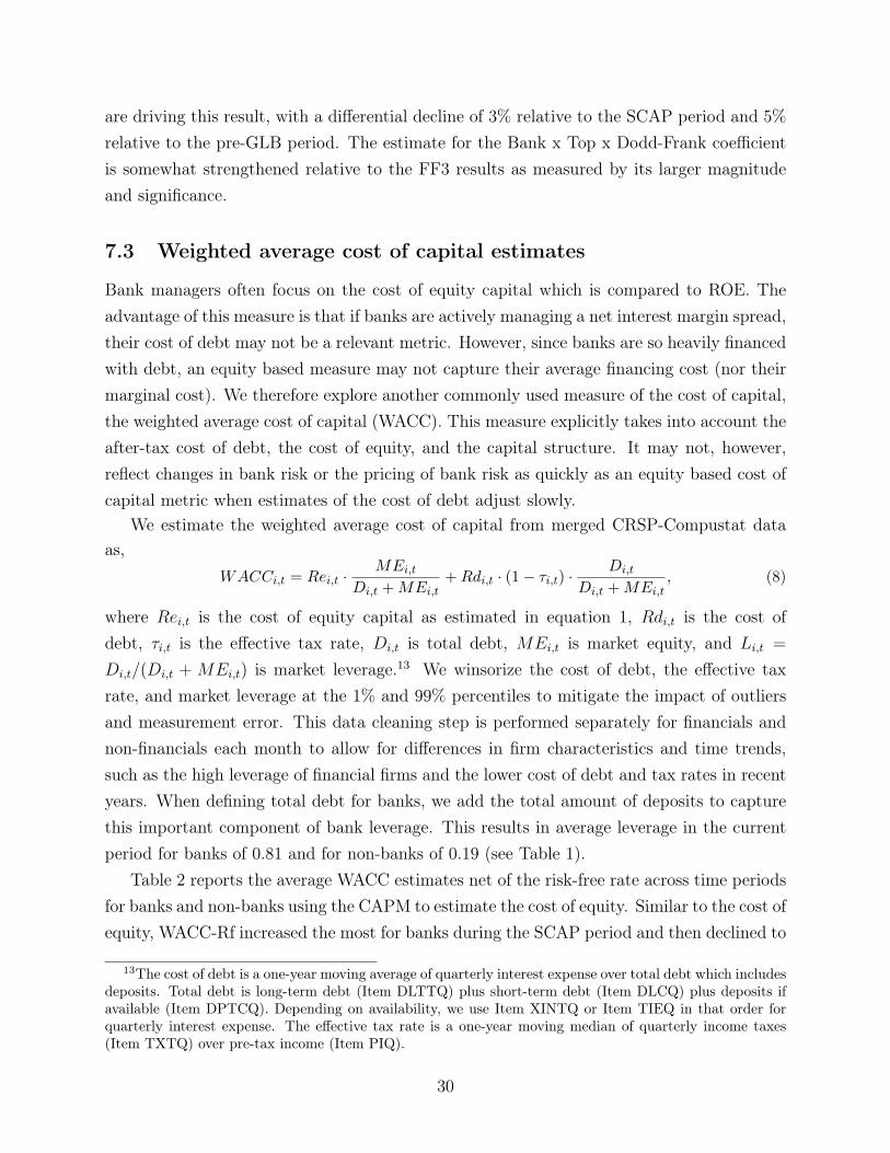
are driving this result, with a differential decline of 3% relative to the SCAP period and 5%relative to the pre-GLB period. The estimate for the Bank x Top x Dodd-Frank coefficientis somewhat strengthened relative to the FF3 results as measured by its larger magnitudeand significance.

7.3 Weighted average cost of capital estimates

Bank managers often focus on the cost of equity capital which is compared to ROE. Theadvantage of this measure is that if banks are actively managing a net interest margin spread,their cost of debt may not be a relevant metric. However, since banks are so heavily financedwith debt, an equity based measure may not capture their average financing cost (nor theirmarginal cost). We therefore explore another commonly used measure of the cost of capital,the weighted average cost of capital (WACC). This measure explicitly takes into account theafter-tax cost of debt, the cost of equity, and the capital structure. It may not, however,reflect changes in bank risk or the pricing of bank risk as quickly as an equity based cost ofcapital metric when estimates of the cost of debt adjust slowly.

We estimate the weighted average cost of capital from merged CRSP-Compustat dataas,

WACCi,t = Rei,t ·MEi,t

Di,t +MEi,t+Rdi,t · (1− τi,t) ·

Di,t

Di,t +MEi,t, (8)

where Rei,t is the cost of equity capital as estimated in equation 1, Rdi,t is the cost ofdebt, τi,t is the effective tax rate, Di,t is total debt, MEi,t is market equity, and Li,t =

Di,t/(Di,t + MEi,t) is market leverage.13 We winsorize the cost of debt, the effective taxrate, and market leverage at the 1% and 99% percentiles to mitigate the impact of outliersand measurement error. This data cleaning step is performed separately for financials andnon-financials each month to allow for differences in firm characteristics and time trends,such as the high leverage of financial firms and the lower cost of debt and tax rates in recentyears. When defining total debt for banks, we add the total amount of deposits to capturethis important component of bank leverage. This results in average leverage in the currentperiod for banks of 0.81 and for non-banks of 0.19 (see Table 1).

Table 2 reports the average WACC estimates net of the risk-free rate across time periodsfor banks and non-banks using the CAPM to estimate the cost of equity. Similar to the cost ofequity, WACC-Rf increased the most for banks during the SCAP period and then declined to

13The cost of debt is a one-year moving average of quarterly interest expense over total debt which includesdeposits. Total debt is long-term debt (Item DLTTQ) plus short-term debt (Item DLCQ) plus deposits ifavailable (Item DPTCQ). Depending on availability, we use Item XINTQ or Item TIEQ in that order forquarterly interest expense. The effective tax rate is a one-year moving median of quarterly income taxes(Item TXTQ) over pre-tax income (Item PIQ).

30

a level above its pre-GLB average. Value-weighted WACC-Rf increased by approximately 2%for banks and 0.7% for non-banks relative to the pre-GLB period. Comparing the SCAP andDodd-Frank periods, value-weighted WACC-Rf decreased by approximately .8% for banksversus an increase of 0.1% for non-banks. Figure 5 illustrates the value-weighted WACCestimate for banks over time using both the CAPM and FF3 models to compute the cost ofequity. While WACC-Rf has increased relative to the pre-GLB period, the overall level ofWACC has been near historical lows during the Dodd-Frank period as a result of the lowrisk-free rate, similar to the cost of equity capital.

The final three columns of Table 8 repeat the difference-in-differences analysis usingWACC-Rf as the dependent variable. One immediate change is that banks’ weighted averagecost of capital is significantly lower than non-banks on average. Bank WACC is almost 6%lower than non-bank WACC as measured by the Bank dummy variable in the value-weightedregression specification 7. This result reflects banks’ use of leverage and the lower cost ofdebt relative to equity financing. It contrasts with the previous finding that banks have ahigher equity cost of capital than non-banks on average. In similarity to the previous results,we do see a decrease in WACC-Rf for banks when comparing the SCAP and Dodd-Frankperiods in specifications 7 and 8. The results comparing the pre-GLB and Dodd-Frankperiods are similar to the CAPM results, featuring a statistically significant increase in thecurrent period by around 1.5%. Finally, we do not find a significant decline in WACC forthe top banks between the SCAP and Dodd-Frank periods in specification 9. This contraststhe estimates of the cost of equity capital for the top banks which have featured a large andsignificant decline across specifications in recent years.

7.4 CAPM with a time-varying equity risk premium

What if the equity risk premium varies over time? Our analysis of the CAPM has assumed aconstant equity risk premium so that time variation in beta captures the change in the costof capital for banks relative to other firms (equation 1). A time varying equity risk premiumthat is correlated with bank betas may bias our results. For example, if bank betas and theequity risk premium are lower in the Dodd-Frank period relative to the SCAP period, thedecline in the cost of capital for banks will be underestimated, all else equal.

To address this concern we consider two approaches. First, we use a model to estimatethe equity risk premium and then repeat our analysis for the CAPM with this time-varyingrisk premium. To do this, we estimate the equity risk premium by projecting one-year aheadreturns for the market onto a one-factor partial least squares estimate that combines 14models of the equity risk premium from Duarte and Rosa (2015) with available data from

31

1965 to 2016.14 This approach has the advantage that it directly addresses the concern thatthe equity risk premium is time varying but the disadvantage that the results are model andsample dependent.

For an alternative perspective, we take advantage of the fact that the equity risk premiumdrops out of a difference-in-differences analysis after taking the logarithm since the CAPMis a one factor model.15 We thus estimate our difference-in-differences regressions using thelogarithm of the CAPM betas as the dependent variable. We implement this idea empiricallyby winsorizing the estimated betas at .05 to remove negative values from the sample.

Table 9 reports the baseline regressions for the CAPM using the partial least squaresestimate of the equity risk premium (denoted PLS-Rf) and for the logarithm of the CAPMbetas.16 For the PLS-Rf regressions almost all of the time period coefficients are largerthan those in the specifications with a constant risk premium. This reflects the fact thatour estimate of the time-varying equity risk premium has increased over the sample period,consistent with the findings in Duarte and Rosa (2015). For banks, the results are generallyconsistent with those from other CAPM specifications, in that the estimated cost of capitalis higher in the Dodd-Frank period relative to the pre-GLB period but significantly lowerthan the SCAP period. Specifications 1 and 2 indicate that the cost of capital for bankshas declined by around 9% from the SCAP period to the Dodd-Frank period both in thecross section and within firm. Specification 3 shows that these results are again driven bythe very largest banks. In comparison to the previous results, the larger magnitudes suggestthat the assumption of a constant equity risk premium may be biasing our results down.Equivalently, the results suggest that bank betas are positively correlated with the equityrisk premium.

Similar results also hold when taking the logarithm of the CAPM betas as the dependentvariable in specifications 4 to 6. For example, specifications 4 and 5 indicate that bankCAPM betas have declined by about 35% from SCAP to Dodd-Frank with much of thedecline being driven by the largest banks. That said, one difference is the negative andsignificant coefficient on Bank x Top x Current in specification 6. This contrasts with thePLS-Rf results in specification 3 but is consistent with the CAPM, three-factor, and five-factor cost of capital estimates using constant factor risk premiums which all indicate thatthe cost of capital for the largest banks has declined relative to both the pre-GLB and SCAP

14Similar results hold by projecting one-year ahead returns onto the estimate of the equity risk premiumfrom a dividend discount model, which is one of the 14 models included in the partial least squares estimate.

15To see this, note that log(βi,tµt) − log(βi,t−1µt−1) − (log(βj,tµt)− log(βj,t−1µt−1)) = log(βi,t) −log(βi,t−1)− (log(βj,t)− log(βj,t−1)) . This argument does not apply to multifactor models.

16The PLS-Rf results are from March 1996 to 2016 when the equity risk premium estimates are availablefrom Duarte and Rosa (2015). This results in a slightly smaller sample and contrasts the other regressionswhich end in 2017.

32

periods on a within firm, value-weighted basis.

7.5 Asset Betas

The key component driving changes in our cost of capital estimates is the estimate of equitybeta. However, we may also be interested in looking directly at asset betas. To do this,we compute asset betas in the Merton (1974) model using equity market capitalization andequity volatility for each firm-month observation in the sample following the approach inBharath and Shumway (2008).17 The advantage of this analysis is that it directly incor-porates leverage into the estimated beta rather than including leverage as a linear controlvariable in reduced form regressions as in Table 4 (specification 5) or in Table 5 (specification6) (where leverage is included as a time-varying characteristic as measured by the Tier 1capital ratio). The disadvantage of this approach is that the computation of asset betas ismodel specific and requires a number of assumptions regarding how to compute the maturityand face value of debt. These assumptions may be particularly important for banks.

7.5.1 Levels of Asset Betas

The final three columns of Table 9 report the results with asset beta as the dependent variablein specifications 7 to 9. The most striking difference from the specifications using the costof capital is the large and negative coefficient on the Bank dummy variable in specification7. Similar to the WACC estimates, banks’ use of leverage significantly lowers asset betasrelative to non-banks which have similar equity betas but much less leverage.18 Looking atthe bank interaction coefficients on the regulatory time periods, we still estimate a significantdecrease in banks’ asset betas between the SCAP and Dodd-Frank periods that is primarilydriven by the very largest banks. This result is noteworthy as the significant decline persistsdespite the decrease in bank leverage in recent years, which would imply increased assetbetas of banks if equity betas were unchanged. From a longer historical perspective, bankasset betas have increased relative to the pre-GLB period by around .10% as measured by the

17We compute asset betas by solving for firm value and volatility from two nonlinear equations for thevalue of equity and equity volatility, similar to how the default probability πsimul

Merton is computed in Bharathand Shumway (2008). To do this we assume that debt matures in one year and define the face value ofdebt as short-term debt plus one-half long-term debt plus deposits if available. In a previous draft we foundsimilar results by assuming that debt was riskless as in Baker and Wurgler (2015) in which case asset betasare equal to βasset

i,t = βi,t(1− Li,t) where Li,t = Di,t/(Di,t +MEi,t).18The average value-weighted bank beta of 1.17 and leverage of .79 corresponds to an asset beta of 1.17

x (1-.79) = .25 for banks using the riskless debt assumption versus an average value-weighted beta of .99for non-banks and leverage of .20 that corresponds to an asset beta of .99 x (1-.20) = .79. This back-of-the-envelope approximation resulting in a difference of -.55 is similar in magnitude to the coefficient of -.60 onthe Bank dummy in specification (7).

33

significant and positive Bank x Top x Dodd-Frank coefficient in specification 9. This resultis similar to the WACC estimates and contrasts the results for the cost of equity capitalestimates, which generally feature a negative difference for the largest banks.

7.5.2 Distribution of Asset Betas

The analysis until now has focused on the mean of banks’ cost of capital, which is drivenby the changes to equity betas, the risk-free rate, the equity risk premium, and leverage.Building on these results, it is also interesting to understand how the distribution of thecost of capital is changing over time. Greenwood et al. (2017) hypothesize that if banks aresubject to multiple capital constraints that the industry will be pushed towards increasinglysimilar business models, particularly for the largest banks. We can test this hypothesis byusing our asset beta estimates as a simple metric to capture the similarity of bank businessmodels. Figure 6 plots the evolution of the distribution of asset betas for the 90 largestbanks. The interquartile range for bank asset betas has averaged approximately 0.08 overthe last 20 years compared to a mean asset beta of 0.20 and a standard deviation of 0.04.While the distribution expanded during the Crisis and SCAP periods, it declined after thepassage of the Dodd-Frank Act to be closer to 0.05. This initial decrease in the distributionof asset betas after the financial crisis is consistent with the hypothesis in Greenwood et al.(2017). However, the trend has reversed in the last years in the sample when the distributionwidened again for the largest 90 banks as reflected in Figure 6.

To compare this result to other industries, Table 10 repeats the difference-in-differencesanalysis from equation 3 at the industry level using the asset beta interquartile range asthe dependent variable in the first four columns and the difference between the 95th and5th percentiles in the last 4 columns. These regressions feature thirteen observations permonth, one for each of the twelve Fama-French industries with financials split into banksand non-bank financials. The first two specifications compute the interquartile range fromthe 90 largest firms by assets for each industry while the second two specifications include allfirms when computing the interquartile range. The Bank indicator coefficient shows that theasset beta distribution of banks is significantly less disperse than that of other industries onaverage. This difference reflects the elevated leverage of banks relative to non-financial firms,resulting in both a lower level of assets betas as discussed previously and a more compresseddistribution as reflected in these results. After accounting for this difference, most of the timeperiod dummies and interaction terms for banks are insignificant. The primary exception isduring the GLB period. If anything, the results suggest that the deregulation of the 2000swas associated with a compression of asset beta distribution for banks relative to non-banks.

34

Over more recent periods, the interquartile range for bank asset betas is not statisticallydistinguishable from the pre-GLB period.

The last four columns report results for the tails of the distribution. If anything, theseregressions suggest a widening of the distribution in recent years. However, given that onlya few firms inform the q95 - q05 quantiles for the 90 largest banks, it is not surprising tosee that most of the coefficients are insignificant, reflecting the significant amount of noisein estimating the tails of the distribution. For the larger sample that includes all banks inspecification 8, the results indicate that the asset beta distribution may have widened outafter the passage of the Dodd-Frank Act, but the magnitude of the change is not as largeas in specification 6. Since the composition of our universe of banks has changed so muchwith the addition of firms such as broker dealers and credit card lenders, we also repeat theanalysis limiting our sample of banks only to those firms that are depository institutions andhave an SIC code beginning with 60. Results are similar (not shown).

8 Conclusion

The cost of capital is important for managers because it represents the rate of return thatmust be earned on investor capital. As a result, banks’ cost of capital is an input intodecisions about lending quantities and pricing as well as decisions regarding asset allocationto different business lines. This paper rigorously estimates the cost of capital for the bankingindustry and explores how it has changed over time. After spiking in the financial crisis,the cost of capital for the banking industry has fallen dramatically since the passage of theDodd-Frank Act. Expected returns for the very largest banks most affected by regulationhave fallen differentially by 1% to 3% relative to post-financial crisis highs depending on themetric. To the extent that the cost of capital is a proxy for equity risk, this means that therisk of these firms has fallen since the passage of the Dodd-Frank Act. For the largest banksin particular, there has been a differential decline in the cost of capital relative to boththe financial crisis and relative to the late 1990s across different measures and regressionspecifications. This is striking in the face of research such as Atkeson et al. (2018) thatsuggests that the value of government guarantees are falling at this time.

While these results suggest that the systematic risk of banks has declined in the postDodd-Frank era, it is worth noting the limitations of any analysis that seeks to understand thecost of capital. The true cost of capital measure relevant to bank managers is the unobservedexpected returns of bank investors. Ultimately, bank managers and econometricians do nothave a time series of expected returns, only the models by which we estimate expectedreturns. Any test is thus a joint test of changes to expected returns and of the model

35

for estimating expected returns. Some issues are alleviated by the differences-in-differencesapproach. For example, the risk-free rate is added to the expected returns and thus dropsout when differencing. Changes in banks’ cost of capital can be compared to other industriesusing different models, even if it is difficult to precisely estimate the level of banks’ cost ofcapital itself.

These questions are not just academic. Our estimates of the cost of capital are capturingchanges in market prices that matter to bank managers. These changes in the cost of capitalare associated with changes in bank lending supply – both in terms of overall conditions,pricing, and quantity.

36

ReferencesAdrian, T., E. Friedman, and T. Muir (2016). The cost of capital of the financial sector. SSRN .

Ang, A. and D. Kristensen (2012). Testing conditional factor models. Journal of FinancialEconomics 106 (1), 132–156.

Atkeson, A. G., A. d’Avernas, A. L. Eisfeldt, and P.-O. Weill (2018). Government guarantees and thevaluation of american banks. NBER Macroeconomics Annual (forthcoming).

Baker, M. and J. Wurgler (2015). Do strict capital requirements raise the cost of capital? bank regulation,capital structure, and the low-risk anomaly. American Economic Review: Papers & Proceedings 105 (5),315–320.

Barber, B. M. and J. D. Lyon (1997). Firm size, book-to-market ratio, and security returns: A holdoutsample of financial firms. The Journal of Finance 52 (2), 875–883.

Berk, J. B. and J. H. van Binsbergen (2016). Assessing asset pricing models using revealed preference.Journal of Financial Economics 119 (1), 1–23.

Bharath, S. T. and T. Shumway (2008). Forecasting default with the merton distance to default model.The Review of Financial Studies 21 (3), 1339–1369.

Brunnermeier, M. K. and Y. Sannikov (2014). A macroeconomic model with a financial sector. AmericanEconomic Review 104 (2), 379–421.

Calomiris, C. W. and D. Nissim (2014). Crisis-related shifts in the market valuation of banking activities.Journal of Financial Intermediation 23, 400–435.

Cochrane, J. H. (2011). Presidential address: Discount rates. The Journal of Finance 66 (4), 1047–1108.

Cummins, J. G., K. A. Hassett, R. G. Hubbard, R. E. Hall, and R. J. Caballero (1994). A reconsiderationof investment behavior using tax reforms as natural experiments. Brookings Papers on EconomicActivity 1994 (2), 1–74.

Duarte, F. and C. Rosa (2015). The equity risk premium: A review of models. Federal Reserve Bank ofNew York Economic Policy Review 21 (2), 39–57.

Fama, E. F. (1970). Efficient capital markets: A review of theory and empirical work. The Journal ofFinance 25 (2), 383–417.

Fama, E. F. (1991). Efficient markets: Ii. The Journal of Finance 46 (5), 1575–1617.

Fama, E. F. and K. R. French (1993). Common risk factors in the returns on stocks and bonds. Journal ofFinancial Economics 33 (1), 3–56.

Fama, E. F. and K. R. French (1997). Industry costs of equity. Journal of Financial Economics 43 (2),153–193.

Flannery, M., B. Hirtle, and A. Kovner (2017). Evaluating the information in the federal reserve stresstests. Journal of Financial Intermediation 29, 1–18.

Frank, M. Z. and T. Shen (2016). Investment and the weighted average cost of capital. Journal ofFinancial Economics 119 (2), 300–315.

Frazzini, A. and L. H. Pedersen (2014). Betting against beta. Journal of Financial Economics 111 (1),1–25.

Gandhi, P. and H. Lustig (2015). Size anomalies in u.s. bank stock returns. The Journal of Finance 70 (2),

37

733–768.

Gilchrist, S., J. W. Sim, and E. Zakrajšek (2013). Misallocation and financial market frictions: Some directevidence from the dispersion in borrowing costs. Review of Economic Dynamics 16 (1), 159–176.

Gilchrist, S. and E. Zakrajšek (2012). Credit spreads and business cycle fluctuations. American EconomicReview 102 (4), 1692–1720.

Graham, J. R. and C. R. Harvey (2001). The theory and practice of corporate finance: evidence from thefield. Journal of Financial Economics 60 (2-3), 187–243.

Greenwood, R., J. C. Stein, S. G. Hanson, and A. Sunderam (2017). Strengthening and streamlining bankcapital regulation. Brookings Papers on Economic Activity 2017 (2), 479–565.

Gurkaynak, R., B. Sack, and J. Wright (2006). The us treasury curve: 1961 to present. Journal ofMonetary Economics 54 (8), 2291–2304.

Hale, G. and J. Santos (2014). Do banks propagate shocks to the debt market? Journal of FinancialEconomic Policy 6 (3), 270–310.

Hou, K., C. Xue, and L. Zhang (2014). Digesting anomalies: An investment approach. Review of FinancialStudies 28 (3), 650–704.

Huizinga, H. and L. Laeven (2012). Bank valuation and accounting discretion during a financial crisis.Journal of Financial Economics 106 (3), 614–634.

King, M. R. (2009). The cost of equity for global banks: a capm perspective from 1990 to 2009. BISQuarterly Review , 59–73.

Lewellen, J. and S. Nagel (2006). The conditional capm does not explain asset-pricing anomalies. Journalof Financial Economics 82 (2), 289–314.

Linnainmaa, J. T. and M. R. Roberts (2016). The history of the cross section of stock returns. SSRN .

Lintner, J. (1965). The valuation of risk assets and the selection of risky investments in stock portfoliosand capital budgets. The Review of Economics and Statistics 47 (1), 13–37.

Lown, C. and D. P. Morgan (2006). The credit cycle and the business cycle: New findings using the loanofficer opinion survey. Journal of Money, Credit and Banking 38 (6), 1575–1597.

Merton, R. C. (1973). An intertemporal capital asset pricing model. Econometrica 41 (5), 867–887.

Merton, R. C. (1974). On the pricing of corporate debt: The risk structure of interest rates. The Journalof Finance 29 (2), 449–470.

Merton, R. C. (1980). On estimating the expected return on the market: An exploratory investigation.Journal of Financial Economics 8 (4), 323–361.

Minton, B. A., R. M. Stulz, and A. G. Taboada (2017). Are larger banks valued more highly? SSRN .

Philippon, T. (2009). The bond market’s q. The Quarterly Journal of Economics 124 (3), 1011–1056.

Ross, S. A. (1976). The arbitrage theory of capital asset pricing. Journal of Economic Theory 13 (3),341–360.

Sarin, N. and L. H. Summers (2016). Understanding bank risk through market measures. Brookings Paperson Economic Activity , 57–127.

Scholes, M. and J. Williams (1977). Estimating betas from nonsynchronous data. Journal of FinancialEconomics 5 (3), 309–327.

38

Schuermann, T. and K. J. Stiroh (2006). Visible and hidden risk factors for banks. Federal Reserve Bank ofNew York Staff Report .

Sharpe, W. F. (1964). Capital asset prices: A theory of market equilibrium under conditions of risk. TheJournal of Finance 19 (3), 425–442.

Welch, I. and A. Goyal (2007). A comprehensive look at the empirical performance of equity premiumprediction. The Review of Financial Studies 21 (4), 1455–1508.

39

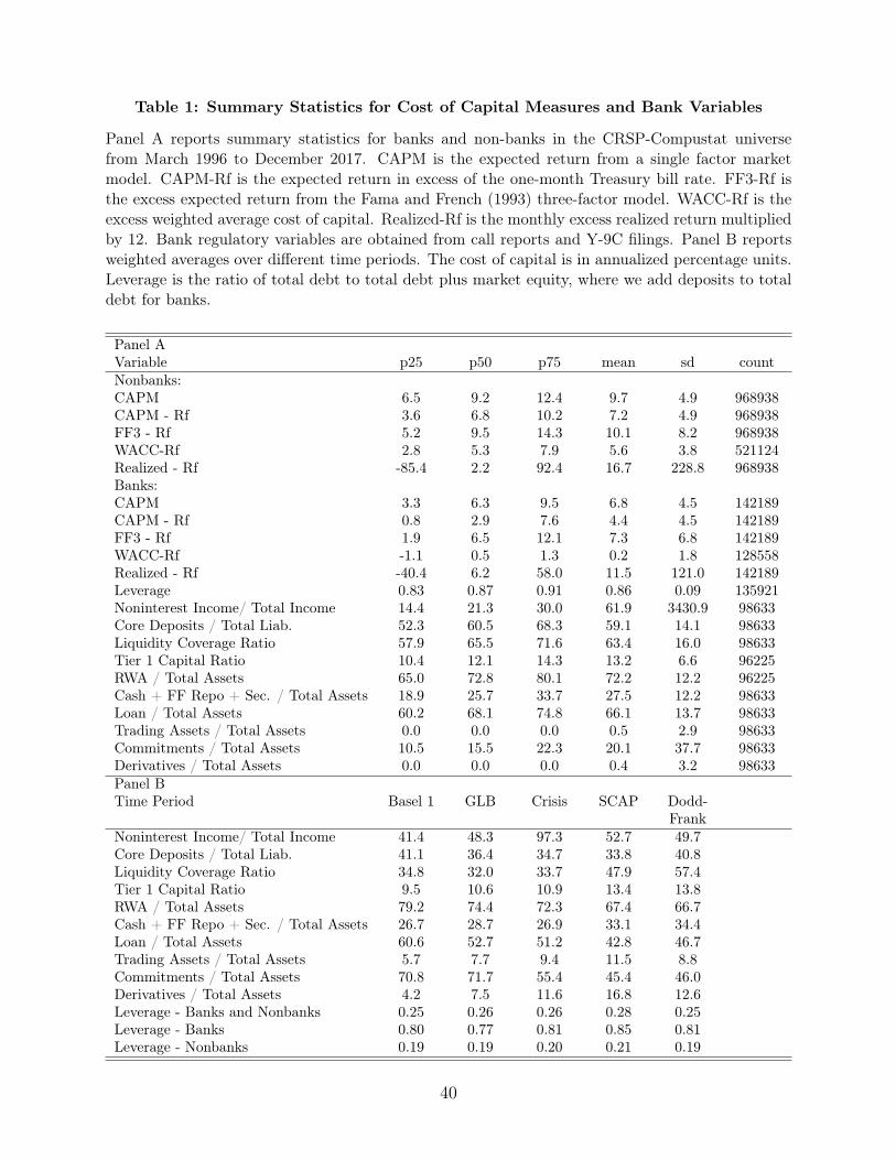
Table 1: Summary Statistics for Cost of Capital Measures and Bank Variables

Panel A reports summary statistics for banks and non-banks in the CRSP-Compustat universefrom March 1996 to December 2017. CAPM is the expected return from a single factor marketmodel. CAPM-Rf is the expected return in excess of the one-month Treasury bill rate. FF3-Rf isthe excess expected return from the Fama and French (1993) three-factor model. WACC-Rf is theexcess weighted average cost of capital. Realized-Rf is the monthly excess realized return multipliedby 12. Bank regulatory variables are obtained from call reports and Y-9C filings. Panel B reportsweighted averages over different time periods. The cost of capital is in annualized percentage units.Leverage is the ratio of total debt to total debt plus market equity, where we add deposits to totaldebt for banks.

Panel AVariable p25 p50 p75 mean sd countNonbanks:CAPM 6.5 9.2 12.4 9.7 4.9 968938CAPM - Rf 3.6 6.8 10.2 7.2 4.9 968938FF3 - Rf 5.2 9.5 14.3 10.1 8.2 968938WACC-Rf 2.8 5.3 7.9 5.6 3.8 521124Realized - Rf -85.4 2.2 92.4 16.7 228.8 968938Banks:CAPM 3.3 6.3 9.5 6.8 4.5 142189CAPM - Rf 0.8 2.9 7.6 4.4 4.5 142189FF3 - Rf 1.9 6.5 12.1 7.3 6.8 142189WACC-Rf -1.1 0.5 1.3 0.2 1.8 128558Realized - Rf -40.4 6.2 58.0 11.5 121.0 142189Leverage 0.83 0.87 0.91 0.86 0.09 135921Noninterest Income/ Total Income 14.4 21.3 30.0 61.9 3430.9 98633Core Deposits / Total Liab. 52.3 60.5 68.3 59.1 14.1 98633Liquidity Coverage Ratio 57.9 65.5 71.6 63.4 16.0 98633Tier 1 Capital Ratio 10.4 12.1 14.3 13.2 6.6 96225RWA / Total Assets 65.0 72.8 80.1 72.2 12.2 96225Cash + FF Repo + Sec. / Total Assets 18.9 25.7 33.7 27.5 12.2 98633Loan / Total Assets 60.2 68.1 74.8 66.1 13.7 98633Trading Assets / Total Assets 0.0 0.0 0.0 0.5 2.9 98633Commitments / Total Assets 10.5 15.5 22.3 20.1 37.7 98633Derivatives / Total Assets 0.0 0.0 0.0 0.4 3.2 98633Panel BTime Period Basel 1 GLB Crisis SCAP Dodd-

FrankNoninterest Income/ Total Income 41.4 48.3 97.3 52.7 49.7Core Deposits / Total Liab. 41.1 36.4 34.7 33.8 40.8Liquidity Coverage Ratio 34.8 32.0 33.7 47.9 57.4Tier 1 Capital Ratio 9.5 10.6 10.9 13.4 13.8RWA / Total Assets 79.2 74.4 72.3 67.4 66.7Cash + FF Repo + Sec. / Total Assets 26.7 28.7 26.9 33.1 34.4Loan / Total Assets 60.6 52.7 51.2 42.8 46.7Trading Assets / Total Assets 5.7 7.7 9.4 11.5 8.8Commitments / Total Assets 70.8 71.7 55.4 45.4 46.0Derivatives / Total Assets 4.2 7.5 11.6 16.8 12.6Leverage - Banks and Nonbanks 0.25 0.26 0.26 0.28 0.25Leverage - Banks 0.80 0.77 0.81 0.85 0.81Leverage - Nonbanks 0.19 0.19 0.20 0.21 0.19

40

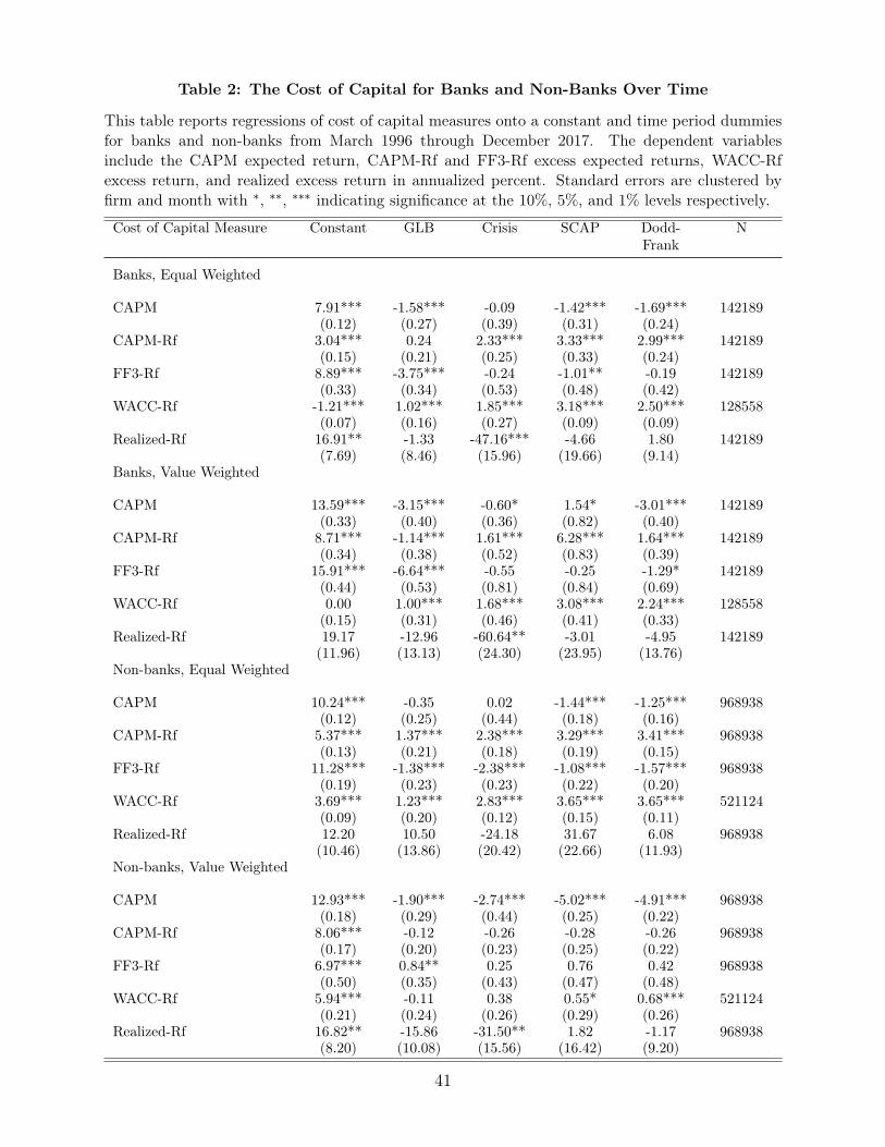
Table 2: The Cost of Capital for Banks and Non-Banks Over Time

This table reports regressions of cost of capital measures onto a constant and time period dummiesfor banks and non-banks from March 1996 through December 2017. The dependent variablesinclude the CAPM expected return, CAPM-Rf and FF3-Rf excess expected returns, WACC-Rfexcess return, and realized excess return in annualized percent. Standard errors are clustered byfirm and month with ∗, ∗∗, ∗∗∗ indicating significance at the 10%, 5%, and 1% levels respectively.

Cost of Capital Measure Constant GLB Crisis SCAP Dodd-Frank

N

Banks, Equal Weighted

CAPM 7.91*** -1.58*** -0.09 -1.42*** -1.69*** 142189(0.12) (0.27) (0.39) (0.31) (0.24)

CAPM-Rf 3.04*** 0.24 2.33*** 3.33*** 2.99*** 142189(0.15) (0.21) (0.25) (0.33) (0.24)

FF3-Rf 8.89*** -3.75*** -0.24 -1.01** -0.19 142189(0.33) (0.34) (0.53) (0.48) (0.42)

WACC-Rf -1.21*** 1.02*** 1.85*** 3.18*** 2.50*** 128558(0.07) (0.16) (0.27) (0.09) (0.09)

Realized-Rf 16.91** -1.33 -47.16*** -4.66 1.80 142189(7.69) (8.46) (15.96) (19.66) (9.14)

Banks, Value Weighted

CAPM 13.59*** -3.15*** -0.60* 1.54* -3.01*** 142189(0.33) (0.40) (0.36) (0.82) (0.40)

CAPM-Rf 8.71*** -1.14*** 1.61*** 6.28*** 1.64*** 142189(0.34) (0.38) (0.52) (0.83) (0.39)

FF3-Rf 15.91*** -6.64*** -0.55 -0.25 -1.29* 142189(0.44) (0.53) (0.81) (0.84) (0.69)

WACC-Rf 0.00 1.00*** 1.68*** 3.08*** 2.24*** 128558(0.15) (0.31) (0.46) (0.41) (0.33)

Realized-Rf 19.17 -12.96 -60.64** -3.01 -4.95 142189(11.96) (13.13) (24.30) (23.95) (13.76)

Non-banks, Equal Weighted

CAPM 10.24*** -0.35 0.02 -1.44*** -1.25*** 968938(0.12) (0.25) (0.44) (0.18) (0.16)

CAPM-Rf 5.37*** 1.37*** 2.38*** 3.29*** 3.41*** 968938(0.13) (0.21) (0.18) (0.19) (0.15)

FF3-Rf 11.28*** -1.38*** -2.38*** -1.08*** -1.57*** 968938(0.19) (0.23) (0.23) (0.22) (0.20)

WACC-Rf 3.69*** 1.23*** 2.83*** 3.65*** 3.65*** 521124(0.09) (0.20) (0.12) (0.15) (0.11)

Realized-Rf 12.20 10.50 -24.18 31.67 6.08 968938(10.46) (13.86) (20.42) (22.66) (11.93)

Non-banks, Value Weighted

CAPM 12.93*** -1.90*** -2.74*** -5.02*** -4.91*** 968938(0.18) (0.29) (0.44) (0.25) (0.22)

CAPM-Rf 8.06*** -0.12 -0.26 -0.28 -0.26 968938(0.17) (0.20) (0.23) (0.25) (0.22)

FF3-Rf 6.97*** 0.84** 0.25 0.76 0.42 968938(0.50) (0.35) (0.43) (0.47) (0.48)

WACC-Rf 5.94*** -0.11 0.38 0.55* 0.68*** 521124(0.21) (0.24) (0.26) (0.29) (0.26)

Realized-Rf 16.82** -15.86 -31.50** 1.82 -1.17 968938(8.20) (10.08) (15.56) (16.42) (9.20)

41

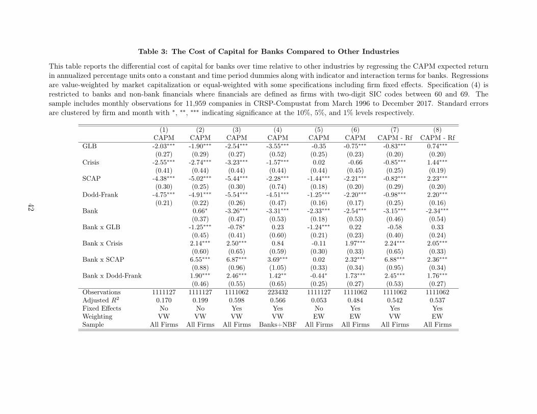
Table 3: The Cost of Capital for Banks Compared to Other Industries

This table reports the differential cost of capital for banks over time relative to other industries by regressing the CAPM expected returnin annualized percentage units onto a constant and time period dummies along with indicator and interaction terms for banks. Regressionsare value-weighted by market capitalization or equal-weighted with some specifications including firm fixed effects. Specification (4) isrestricted to banks and non-bank financials where financials are defined as firms with two-digit SIC codes between 60 and 69. Thesample includes monthly observations for 11,959 companies in CRSP-Compustat from March 1996 to December 2017. Standard errorsare clustered by firm and month with ∗, ∗∗, ∗∗∗ indicating significance at the 10%, 5%, and 1% levels respectively.

(1) (2) (3) (4) (5) (6) (7) (8)CAPM CAPM CAPM CAPM CAPM CAPM CAPM - Rf CAPM - Rf

GLB -2.03∗∗∗ -1.90∗∗∗ -2.54∗∗∗ -3.55∗∗∗ -0.35 -0.75∗∗∗ -0.83∗∗∗ 0.74∗∗∗(0.27) (0.29) (0.27) (0.52) (0.25) (0.23) (0.20) (0.20)

Crisis -2.55∗∗∗ -2.74∗∗∗ -3.23∗∗∗ -1.57∗∗∗ 0.02 -0.66 -0.85∗∗∗ 1.44∗∗∗(0.41) (0.44) (0.44) (0.44) (0.44) (0.45) (0.25) (0.19)

SCAP -4.38∗∗∗ -5.02∗∗∗ -5.44∗∗∗ -2.28∗∗∗ -1.44∗∗∗ -2.21∗∗∗ -0.82∗∗∗ 2.23∗∗∗(0.30) (0.25) (0.30) (0.74) (0.18) (0.20) (0.29) (0.20)

Dodd-Frank -4.75∗∗∗ -4.91∗∗∗ -5.54∗∗∗ -4.51∗∗∗ -1.25∗∗∗ -2.20∗∗∗ -0.98∗∗∗ 2.20∗∗∗(0.21) (0.22) (0.26) (0.47) (0.16) (0.17) (0.25) (0.16)

Bank 0.66∗ -3.26∗∗∗ -3.31∗∗∗ -2.33∗∗∗ -2.54∗∗∗ -3.15∗∗∗ -2.34∗∗∗(0.37) (0.47) (0.53) (0.18) (0.53) (0.46) (0.54)

Bank x GLB -1.25∗∗∗ -0.78∗ 0.23 -1.24∗∗∗ 0.22 -0.58 0.33(0.45) (0.41) (0.60) (0.21) (0.23) (0.40) (0.24)

Bank x Crisis 2.14∗∗∗ 2.50∗∗∗ 0.84 -0.11 1.97∗∗∗ 2.24∗∗∗ 2.05∗∗∗(0.60) (0.65) (0.59) (0.30) (0.33) (0.65) (0.33)

Bank x SCAP 6.55∗∗∗ 6.87∗∗∗ 3.69∗∗∗ 0.02 2.32∗∗∗ 6.88∗∗∗ 2.36∗∗∗(0.88) (0.96) (1.05) (0.33) (0.34) (0.95) (0.34)

Bank x Dodd-Frank 1.90∗∗∗ 2.46∗∗∗ 1.42∗∗ -0.44∗ 1.73∗∗∗ 2.45∗∗∗ 1.76∗∗∗(0.46) (0.55) (0.65) (0.25) (0.27) (0.53) (0.27)

Observations 1111127 1111127 1111062 223432 1111127 1111062 1111062 1111062Adjusted R2 0.170 0.199 0.598 0.566 0.053 0.484 0.542 0.537Fixed Effects No No Yes Yes No Yes Yes YesWeighting VW VW VW VW EW EW VW EWSample All Firms All Firms All Firms Banks+NBF All Firms All Firms All Firms All Firms

42

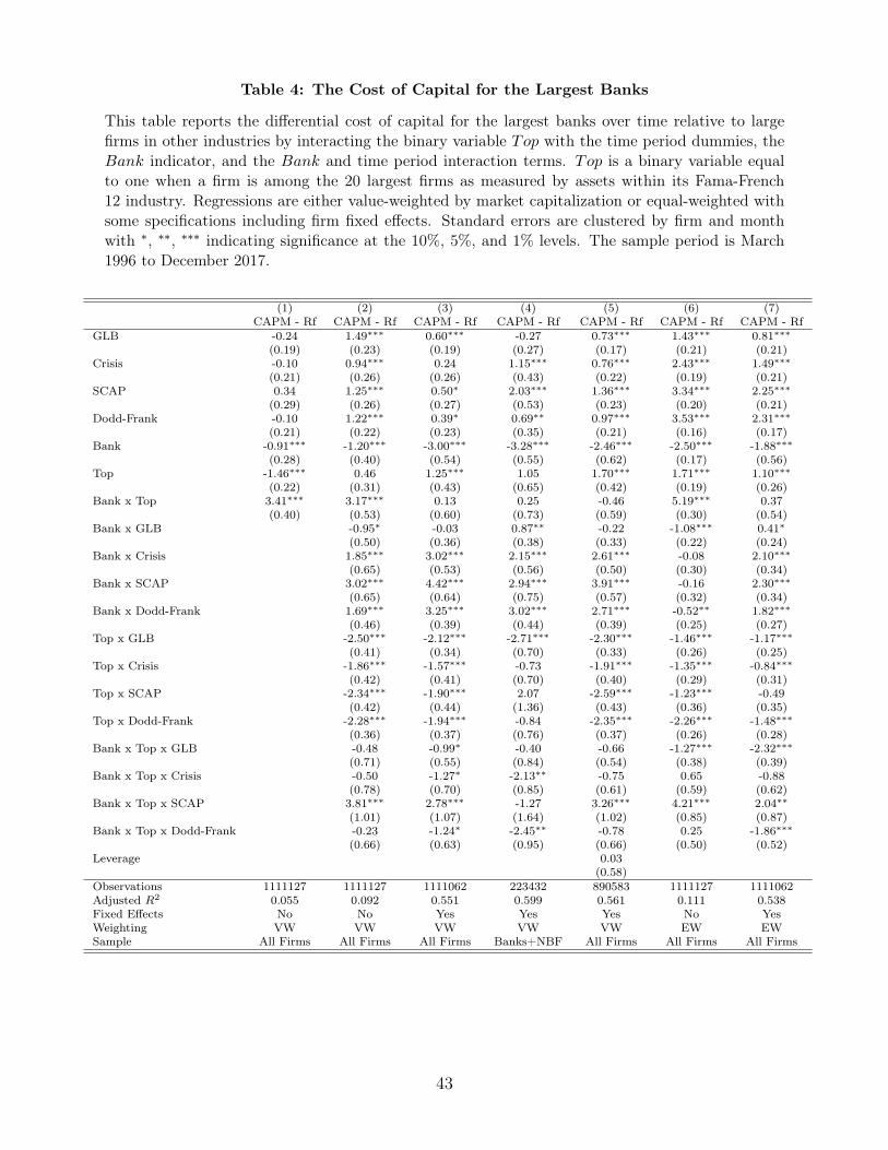
Table 4: The Cost of Capital for the Largest Banks

This table reports the differential cost of capital for the largest banks over time relative to largefirms in other industries by interacting the binary variable Top with the time period dummies, theBank indicator, and the Bank and time period interaction terms. Top is a binary variable equalto one when a firm is among the 20 largest firms as measured by assets within its Fama-French12 industry. Regressions are either value-weighted by market capitalization or equal-weighted withsome specifications including firm fixed effects. Standard errors are clustered by firm and monthwith ∗, ∗∗, ∗∗∗ indicating significance at the 10%, 5%, and 1% levels. The sample period is March1996 to December 2017.

(1) (2) (3) (4) (5) (6) (7)CAPM - Rf CAPM - Rf CAPM - Rf CAPM - Rf CAPM - Rf CAPM - Rf CAPM - Rf

GLB -0.24 1.49∗∗∗ 0.60∗∗∗ -0.27 0.73∗∗∗ 1.43∗∗∗ 0.81∗∗∗(0.19) (0.23) (0.19) (0.27) (0.17) (0.21) (0.21)

Crisis -0.10 0.94∗∗∗ 0.24 1.15∗∗∗ 0.76∗∗∗ 2.43∗∗∗ 1.49∗∗∗(0.21) (0.26) (0.26) (0.43) (0.22) (0.19) (0.21)

SCAP 0.34 1.25∗∗∗ 0.50∗ 2.03∗∗∗ 1.36∗∗∗ 3.34∗∗∗ 2.25∗∗∗(0.29) (0.26) (0.27) (0.53) (0.23) (0.20) (0.21)

Dodd-Frank -0.10 1.22∗∗∗ 0.39∗ 0.69∗∗ 0.97∗∗∗ 3.53∗∗∗ 2.31∗∗∗(0.21) (0.22) (0.23) (0.35) (0.21) (0.16) (0.17)

Bank -0.91∗∗∗ -1.20∗∗∗ -3.00∗∗∗ -3.28∗∗∗ -2.46∗∗∗ -2.50∗∗∗ -1.88∗∗∗(0.28) (0.40) (0.54) (0.55) (0.62) (0.17) (0.56)

Top -1.46∗∗∗ 0.46 1.25∗∗∗ 1.05 1.70∗∗∗ 1.71∗∗∗ 1.10∗∗∗(0.22) (0.31) (0.43) (0.65) (0.42) (0.19) (0.26)

Bank x Top 3.41∗∗∗ 3.17∗∗∗ 0.13 0.25 -0.46 5.19∗∗∗ 0.37(0.40) (0.53) (0.60) (0.73) (0.59) (0.30) (0.54)

Bank x GLB -0.95∗ -0.03 0.87∗∗ -0.22 -1.08∗∗∗ 0.41∗(0.50) (0.36) (0.38) (0.33) (0.22) (0.24)

Bank x Crisis 1.85∗∗∗ 3.02∗∗∗ 2.15∗∗∗ 2.61∗∗∗ -0.08 2.10∗∗∗(0.65) (0.53) (0.56) (0.50) (0.30) (0.34)

Bank x SCAP 3.02∗∗∗ 4.42∗∗∗ 2.94∗∗∗ 3.91∗∗∗ -0.16 2.30∗∗∗(0.65) (0.64) (0.75) (0.57) (0.32) (0.34)

Bank x Dodd-Frank 1.69∗∗∗ 3.25∗∗∗ 3.02∗∗∗ 2.71∗∗∗ -0.52∗∗ 1.82∗∗∗(0.46) (0.39) (0.44) (0.39) (0.25) (0.27)

Top x GLB -2.50∗∗∗ -2.12∗∗∗ -2.71∗∗∗ -2.30∗∗∗ -1.46∗∗∗ -1.17∗∗∗(0.41) (0.34) (0.70) (0.33) (0.26) (0.25)

Top x Crisis -1.86∗∗∗ -1.57∗∗∗ -0.73 -1.91∗∗∗ -1.35∗∗∗ -0.84∗∗∗(0.42) (0.41) (0.70) (0.40) (0.29) (0.31)

Top x SCAP -2.34∗∗∗ -1.90∗∗∗ 2.07 -2.59∗∗∗ -1.23∗∗∗ -0.49(0.42) (0.44) (1.36) (0.43) (0.36) (0.35)

Top x Dodd-Frank -2.28∗∗∗ -1.94∗∗∗ -0.84 -2.35∗∗∗ -2.26∗∗∗ -1.48∗∗∗(0.36) (0.37) (0.76) (0.37) (0.26) (0.28)

Bank x Top x GLB -0.48 -0.99∗ -0.40 -0.66 -1.27∗∗∗ -2.32∗∗∗(0.71) (0.55) (0.84) (0.54) (0.38) (0.39)

Bank x Top x Crisis -0.50 -1.27∗ -2.13∗∗ -0.75 0.65 -0.88(0.78) (0.70) (0.85) (0.61) (0.59) (0.62)

Bank x Top x SCAP 3.81∗∗∗ 2.78∗∗∗ -1.27 3.26∗∗∗ 4.21∗∗∗ 2.04∗∗(1.01) (1.07) (1.64) (1.02) (0.85) (0.87)

Bank x Top x Dodd-Frank -0.23 -1.24∗ -2.45∗∗ -0.78 0.25 -1.86∗∗∗(0.66) (0.63) (0.95) (0.66) (0.50) (0.52)

Leverage 0.03(0.58)

Observations 1111127 1111127 1111062 223432 890583 1111127 1111062Adjusted R2 0.055 0.092 0.551 0.599 0.561 0.111 0.538Fixed Effects No No Yes Yes Yes No YesWeighting VW VW VW VW VW EW EWSample All Firms All Firms All Firms Banks+NBF All Firms All Firms All Firms

43

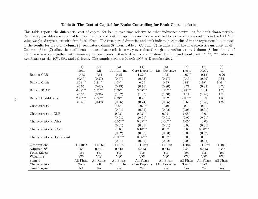
Table 5: The Cost of Capital for Banks Controlling for Bank Characteristics

This table reports the differential cost of capital for banks over time relative to other industries controlling for bank characteristics.Regulatory variables are obtained from call reports and Y-9C filings. The results are reported for expected excess returns in the CAPM invalue-weighted regressions with firm fixed effects. The time period dummies and bank indicator are included in the regressions but omittedin the results for brevity. Column (1) replicates column (8) from Table 3. Column (2) includes all of the characteristics unconditionally.Columns (3) to (7) allow the coefficients on each characteristic to vary over time through interaction terms. Column (8) includes all ofthe characteristics together with time-varying coefficients. Standard errors are clustered by firm and month with ∗, ∗∗, ∗∗∗ indicatingsignificance at the 10%, 5%, and 1% levels. The sample period is March 1996 to December 2017.

(1) (2) (3) (4) (5) (6) (7) (8)None All Non Int. Inc. Core Deposits Liq. Coverage Tier 1 RWA All

Bank x GLB -0.58 -0.61 0.45 -1.82∗∗∗ -1.05∗∗ -1.07∗∗ 0.12 -0.20(0.40) (0.37) (0.57) (0.53) (0.47) (0.46) (0.59) (0.51)

Bank x Crisis 2.24∗∗∗ 2.24∗∗∗ 4.03∗∗∗ 0.35 0.95 1.74∗∗ 2.28∗∗∗ 2.32∗∗∗(0.65) (0.62) (0.79) (0.76) (0.80) (0.71) (0.83) (0.78)

Bank x SCAP 6.88∗∗∗ 6.76∗∗∗ 7.79∗∗∗ 3.48∗∗∗ 4.91∗∗∗ 6.87∗∗∗ 1.64 1.73(0.95) (0.95) (1.22) (1.07) (1.50) (1.11) (1.48) (1.26)

Bank x Dodd-Frank 2.45∗∗∗ 2.32∗∗∗ 4.38∗∗∗ 0.26 0.82 2.03∗∗∗ 1.89 1.36(0.53) (0.49) (0.66) (0.74) (0.95) (0.65) (1.28) (1.22)

Characteristic 0.05∗∗∗ -0.07∗∗∗ -0.01 -0.01 0.01(0.01) (0.02) (0.02) (0.03) (0.01)

Characteristic x GLB -0.03∗∗ 0.03∗∗∗ 0.02∗ 0.05∗ -0.01(0.01) (0.01) (0.01) (0.03) (0.01)

Characteristic x Crisis -0.05∗∗∗ 0.05∗∗∗ 0.04∗∗∗ 0.05∗ -0.00(0.01) (0.01) (0.01) (0.03) (0.01)

Characteristic x SCAP -0.03 0.10∗∗∗ 0.05∗ 0.00 0.08∗∗∗(0.02) (0.02) (0.03) (0.03) (0.02)

Characteristic x Dodd-Frank -0.05∗∗∗ 0.06∗∗∗ 0.03∗ 0.03 0.01(0.01) (0.01) (0.02) (0.03) (0.02)

Observations 1111062 1111062 1111062 1111062 1111062 1111062 1111062 1111062Adjusted R2 0.542 0.543 0.542 0.543 0.543 0.542 0.543 0.546Fixed Effects Yes Yes Yes Yes Yes Yes Yes YesWeighting VW VW VW VW VW VW VW VWSample All Firms All Firms All Firms All Firms All Firms All Firms All Firms All FirmsCharacteristic None All Non Int. Inc. Core Deposits Liq. Coverage Tier 1 RWA AllTime Varying NA No Yes Yes Yes Yes Yes Yes

44

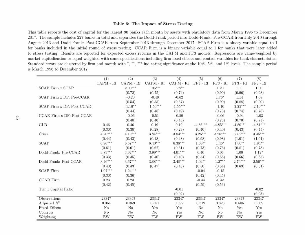
Table 6: The Impact of Stress Testing

This table reports the cost of capital for the largest 90 banks each month by assets with regulatory data from March 1996 to December2017. The sample includes 227 banks in total and separates the Dodd-Frank period into Dodd-Frank: Pre-CCAR from July 2010 throughAugust 2013 and Dodd-Frank: Post-CCAR from September 2013 through December 2017. SCAP Firm is a binary variable equal to 1for banks included in the initial round of stress testing. CCAR Firm is a binary variable equal to 1 for banks that were later addedto stress testing. Results are reported for expected excess returns in the CAPM and FF3 models. Regressions are value-weighted bymarket capitalization or equal-weighted with some specifications including firm fixed effects and control variables for bank characteristics.Standard errors are clustered by firm and month with ∗, ∗∗, ∗∗∗ indicating significance at the 10%, 5%, and 1% levels. The sample periodis March 1996 to December 2017.

(1) (2) (3) (4) (5) (6) (7) (8)CAPM - Rf CAPM - Rf CAPM - Rf CAPM - Rf FF3 - Rf FF3 - Rf FF3 - Rf FF3 - Rf

SCAP Firm x SCAP 2.00∗∗∗ 1.95∗∗∗ 1.78∗∗ 1.20 1.11 1.00(0.72) (0.75) (0.74) (0.90) (0.96) (0.98)

SCAP Firm x DF: Pre-CCAR -0.20 -0.49 -0.62 1.76∗ 1.14 1.08(0.54) (0.55) (0.57) (0.90) (0.88) (0.90)

SCAP Firm x DF: Post-CCAR -1.10∗∗ -1.50∗∗∗ -1.55∗∗∗ -1.10 -2.25∗∗∗ -2.19∗∗∗(0.44) (0.48) (0.49) (0.73) (0.74) (0.78)

CCAR Firm x DF: Post-CCAR -0.06 -0.51 -0.59 -0.06 -0.94 -1.03(0.40) (0.40) (0.43) (0.75) (0.70) (0.73)

GLB 0.46 0.46 0.19 0.19 -4.86∗∗∗ -4.85∗∗∗ -4.80∗∗∗ -4.81∗∗∗(0.30) (0.30) (0.28) (0.29) (0.40) (0.40) (0.43) (0.45)

Crisis 4.20∗∗∗ 4.19∗∗∗ 3.84∗∗∗ 3.84∗∗∗ 3.26∗∗∗ 3.26∗∗∗ 3.45∗∗∗ 3.46∗∗∗(0.44) (0.43) (0.48) (0.48) (0.98) (0.98) (1.01) (1.01)

SCAP 6.96∗∗∗ 6.57∗∗∗ 6.40∗∗∗ 6.38∗∗∗ 1.68∗∗ 1.46∗ 1.86∗∗ 1.94∗∗(0.61) (0.61) (0.62) (0.61) (0.73) (0.76) (0.81) (0.78)

Dodd-Frank: Pre-CCAR 3.89∗∗∗ 3.92∗∗∗ 3.99∗∗∗ 4.01∗∗∗ 0.40 0.06 1.00 1.12∗(0.33) (0.35) (0.40) (0.40) (0.54) (0.56) (0.66) (0.65)

Dodd-Frank: Post-CCAR 3.46∗∗∗ 3.67∗∗∗ 3.88∗∗∗ 3.48∗∗∗ 1.04∗∗ 1.27∗∗ 2.76∗∗∗ 2.56∗∗∗(0.40) (0.43) (0.47) (0.43) (0.50) (0.54) (0.63) (0.61)

SCAP Firm 1.07∗∗∗ 1.24∗∗∗ -0.04 -0.15(0.30) (0.36) (0.42) (0.45)

CCAR Firm 0.23 0.23 -0.44 -0.43(0.42) (0.45) (0.59) (0.53)

Tier 1 Capital Ratio -0.01 -0.02(0.02) (0.03)

Observations 23347 23347 23347 23347 23347 23347 23347 23347Adjusted R2 0.364 0.369 0.581 0.592 0.319 0.323 0.506 0.509Fixed Effects No No Yes Yes No No Yes YesControls No No No Yes No No No YesWeighting EW EW EW EW EW EW EW EW

45

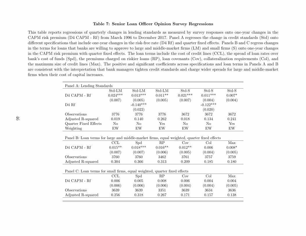
Table 7: Senior Loan Officer Opinion Survey Regressions

This table reports regressions of quarterly changes in lending standards as measured by survey responses onto one-year changes in theCAPM risk premium (D4 CAPM - Rf) from March 1996 to December 2017. Panel A regresses the change in credit standards (Std) ontodifferent specifications that include one-year changes in the risk-free rate (D4 Rf) and quarter fixed effects. Panels B and C regress changesin the terms for loans that banks are willing to approve to large and middle-market firms (LM) and small firms (S) onto one-year changesin the CAPM risk premium with quarter fixed effects. The loan terms include the cost of credit lines (CCL), the spread of loan rates overbank’s cost of funds (Spd), the premiums charged on riskier loans (RP), loan covenants (Cov), collateralization requirements (Col), andthe maximum size of credit lines (Max). The positive and significant coefficients across specifications and loan terms in Panels A and Bare consistent with the interpretation that bank managers tighten credit standards and charge wider spreads for large and middle-marketfirms when their cost of capital increases.

Panel A: Lending StandardsStd-LM Std-LM Std-LM Std-S Std-S Std-S

D4 CAPM - Rf 0.024*** 0.013*** 0.011** 0.021*** 0.011*** 0.007*(0.007) (0.005) (0.005) (0.007) (0.004) (0.004)

D4 Rf -0.140*** -0.122***(0.022) (0.020)

Observations 3776 3776 3776 3672 3672 3672Adjusted R-squared 0.019 0.140 0.262 0.018 0.134 0.241Quarter Fixed Effects No No Yes No No YesWeighting EW EW EW EW EW EW

Panel B: Loan terms for large and middle-market firms, equal weighted, quarter fixed effectsCCL Spd RP Cov Col Max

D4 CAPM - Rf 0.015** 0.018*** 0.016** 0.012** 0.006 0.008*(0.007) (0.007) (0.006) (0.005) (0.004) (0.005)

Observations 3760 3760 3462 3761 3757 3759Adjusted R-squared 0.304 0.366 0.313 0.209 0.185 0.180

Panel C: Loan terms for small firms, equal weighted, quarter fixed effectsCCL Spd RP Cov Col Max

D4 CAPM - Rf 0.006 0.005 0.008 0.006 0.004 0.004(0.006) (0.006) (0.006) (0.004) (0.004) (0.005)

Observations 3639 3639 3351 3639 3634 3636Adjusted R-squared 0.256 0.318 0.267 0.171 0.157 0.138

46

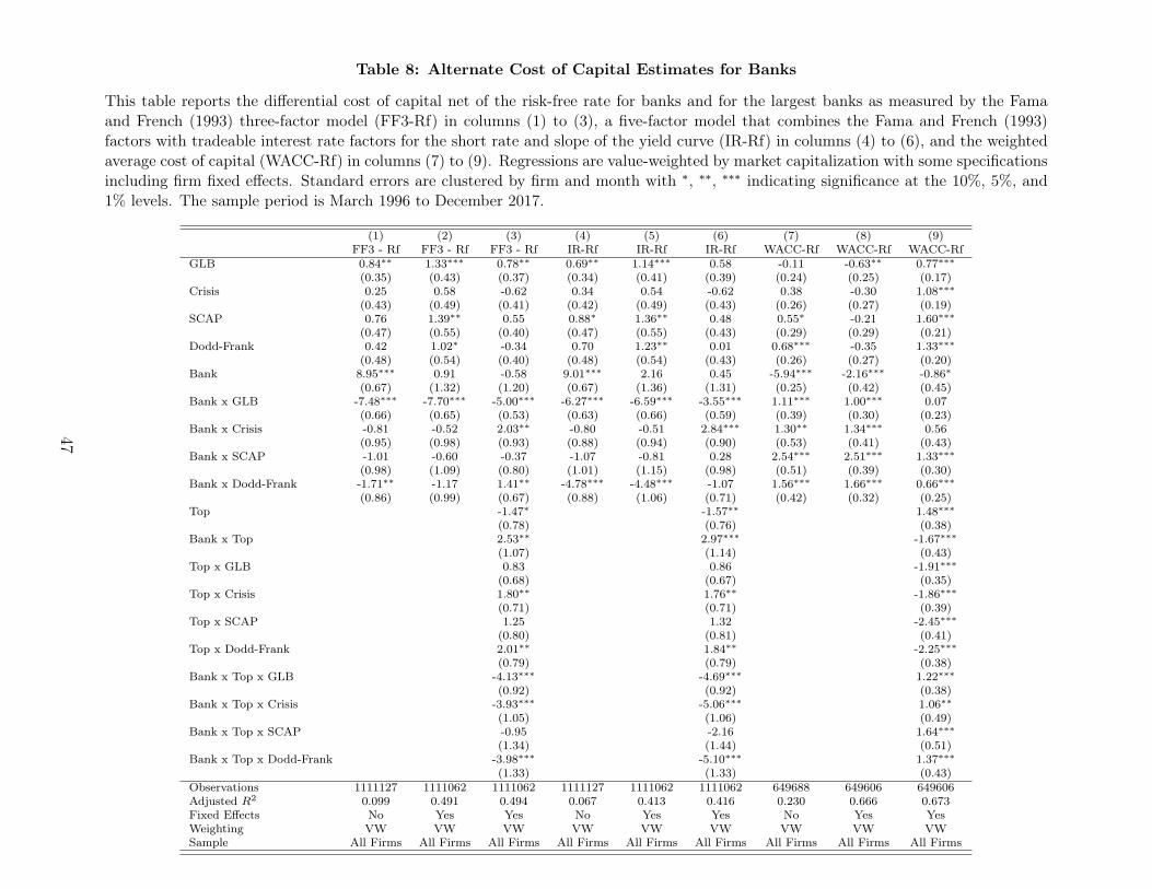
Table 8: Alternate Cost of Capital Estimates for Banks

This table reports the differential cost of capital net of the risk-free rate for banks and for the largest banks as measured by the Famaand French (1993) three-factor model (FF3-Rf) in columns (1) to (3), a five-factor model that combines the Fama and French (1993)factors with tradeable interest rate factors for the short rate and slope of the yield curve (IR-Rf) in columns (4) to (6), and the weightedaverage cost of capital (WACC-Rf) in columns (7) to (9). Regressions are value-weighted by market capitalization with some specificationsincluding firm fixed effects. Standard errors are clustered by firm and month with ∗, ∗∗, ∗∗∗ indicating significance at the 10%, 5%, and1% levels. The sample period is March 1996 to December 2017.

(1) (2) (3) (4) (5) (6) (7) (8) (9)FF3 - Rf FF3 - Rf FF3 - Rf IR-Rf IR-Rf IR-Rf WACC-Rf WACC-Rf WACC-Rf

GLB 0.84∗∗ 1.33∗∗∗ 0.78∗∗ 0.69∗∗ 1.14∗∗∗ 0.58 -0.11 -0.63∗∗ 0.77∗∗∗(0.35) (0.43) (0.37) (0.34) (0.41) (0.39) (0.24) (0.25) (0.17)

Crisis 0.25 0.58 -0.62 0.34 0.54 -0.62 0.38 -0.30 1.08∗∗∗(0.43) (0.49) (0.41) (0.42) (0.49) (0.43) (0.26) (0.27) (0.19)

SCAP 0.76 1.39∗∗ 0.55 0.88∗ 1.36∗∗ 0.48 0.55∗ -0.21 1.60∗∗∗(0.47) (0.55) (0.40) (0.47) (0.55) (0.43) (0.29) (0.29) (0.21)

Dodd-Frank 0.42 1.02∗ -0.34 0.70 1.23∗∗ 0.01 0.68∗∗∗ -0.35 1.33∗∗∗(0.48) (0.54) (0.40) (0.48) (0.54) (0.43) (0.26) (0.27) (0.20)

Bank 8.95∗∗∗ 0.91 -0.58 9.01∗∗∗ 2.16 0.45 -5.94∗∗∗ -2.16∗∗∗ -0.86∗(0.67) (1.32) (1.20) (0.67) (1.36) (1.31) (0.25) (0.42) (0.45)

Bank x GLB -7.48∗∗∗ -7.70∗∗∗ -5.00∗∗∗ -6.27∗∗∗ -6.59∗∗∗ -3.55∗∗∗ 1.11∗∗∗ 1.00∗∗∗ 0.07(0.66) (0.65) (0.53) (0.63) (0.66) (0.59) (0.39) (0.30) (0.23)

Bank x Crisis -0.81 -0.52 2.03∗∗ -0.80 -0.51 2.84∗∗∗ 1.30∗∗ 1.34∗∗∗ 0.56(0.95) (0.98) (0.93) (0.88) (0.94) (0.90) (0.53) (0.41) (0.43)

Bank x SCAP -1.01 -0.60 -0.37 -1.07 -0.81 0.28 2.54∗∗∗ 2.51∗∗∗ 1.33∗∗∗(0.98) (1.09) (0.80) (1.01) (1.15) (0.98) (0.51) (0.39) (0.30)

Bank x Dodd-Frank -1.71∗∗ -1.17 1.41∗∗ -4.78∗∗∗ -4.48∗∗∗ -1.07 1.56∗∗∗ 1.66∗∗∗ 0.66∗∗∗(0.86) (0.99) (0.67) (0.88) (1.06) (0.71) (0.42) (0.32) (0.25)

Top -1.47∗ -1.57∗∗ 1.48∗∗∗(0.78) (0.76) (0.38)

Bank x Top 2.53∗∗ 2.97∗∗∗ -1.67∗∗∗(1.07) (1.14) (0.43)

Top x GLB 0.83 0.86 -1.91∗∗∗(0.68) (0.67) (0.35)

Top x Crisis 1.80∗∗ 1.76∗∗ -1.86∗∗∗(0.71) (0.71) (0.39)

Top x SCAP 1.25 1.32 -2.45∗∗∗(0.80) (0.81) (0.41)

Top x Dodd-Frank 2.01∗∗ 1.84∗∗ -2.25∗∗∗(0.79) (0.79) (0.38)

Bank x Top x GLB -4.13∗∗∗ -4.69∗∗∗ 1.22∗∗∗(0.92) (0.92) (0.38)

Bank x Top x Crisis -3.93∗∗∗ -5.06∗∗∗ 1.06∗∗(1.05) (1.06) (0.49)

Bank x Top x SCAP -0.95 -2.16 1.64∗∗∗(1.34) (1.44) (0.51)

Bank x Top x Dodd-Frank -3.98∗∗∗ -5.10∗∗∗ 1.37∗∗∗(1.33) (1.33) (0.43)

Observations 1111127 1111062 1111062 1111127 1111062 1111062 649688 649606 649606Adjusted R2 0.099 0.491 0.494 0.067 0.413 0.416 0.230 0.666 0.673Fixed Effects No Yes Yes No Yes Yes No Yes YesWeighting VW VW VW VW VW VW VW VW VWSample All Firms All Firms All Firms All Firms All Firms All Firms All Firms All Firms All Firms

47

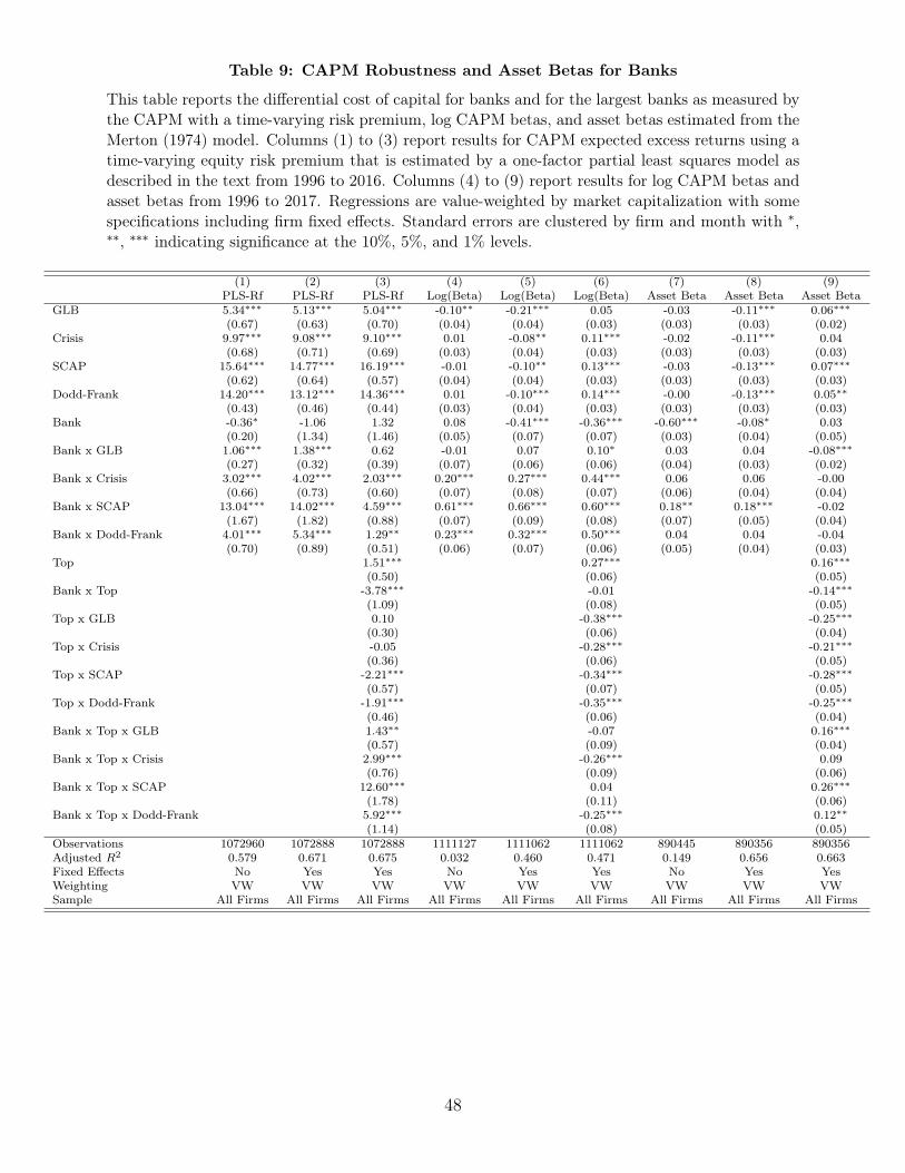
Table 9: CAPM Robustness and Asset Betas for Banks

This table reports the differential cost of capital for banks and for the largest banks as measured bythe CAPM with a time-varying risk premium, log CAPM betas, and asset betas estimated from theMerton (1974) model. Columns (1) to (3) report results for CAPM expected excess returns using atime-varying equity risk premium that is estimated by a one-factor partial least squares model asdescribed in the text from 1996 to 2016. Columns (4) to (9) report results for log CAPM betas andasset betas from 1996 to 2017. Regressions are value-weighted by market capitalization with somespecifications including firm fixed effects. Standard errors are clustered by firm and month with ∗,∗∗, ∗∗∗ indicating significance at the 10%, 5%, and 1% levels.

(1) (2) (3) (4) (5) (6) (7) (8) (9)PLS-Rf PLS-Rf PLS-Rf Log(Beta) Log(Beta) Log(Beta) Asset Beta Asset Beta Asset Beta

GLB 5.34∗∗∗ 5.13∗∗∗ 5.04∗∗∗ -0.10∗∗ -0.21∗∗∗ 0.05 -0.03 -0.11∗∗∗ 0.06∗∗∗(0.67) (0.63) (0.70) (0.04) (0.04) (0.03) (0.03) (0.03) (0.02)

Crisis 9.97∗∗∗ 9.08∗∗∗ 9.10∗∗∗ 0.01 -0.08∗∗ 0.11∗∗∗ -0.02 -0.11∗∗∗ 0.04(0.68) (0.71) (0.69) (0.03) (0.04) (0.03) (0.03) (0.03) (0.03)

SCAP 15.64∗∗∗ 14.77∗∗∗ 16.19∗∗∗ -0.01 -0.10∗∗ 0.13∗∗∗ -0.03 -0.13∗∗∗ 0.07∗∗∗(0.62) (0.64) (0.57) (0.04) (0.04) (0.03) (0.03) (0.03) (0.03)

Dodd-Frank 14.20∗∗∗ 13.12∗∗∗ 14.36∗∗∗ 0.01 -0.10∗∗∗ 0.14∗∗∗ -0.00 -0.13∗∗∗ 0.05∗∗(0.43) (0.46) (0.44) (0.03) (0.04) (0.03) (0.03) (0.03) (0.03)

Bank -0.36∗ -1.06 1.32 0.08 -0.41∗∗∗ -0.36∗∗∗ -0.60∗∗∗ -0.08∗ 0.03(0.20) (1.34) (1.46) (0.05) (0.07) (0.07) (0.03) (0.04) (0.05)

Bank x GLB 1.06∗∗∗ 1.38∗∗∗ 0.62 -0.01 0.07 0.10∗ 0.03 0.04 -0.08∗∗∗(0.27) (0.32) (0.39) (0.07) (0.06) (0.06) (0.04) (0.03) (0.02)

Bank x Crisis 3.02∗∗∗ 4.02∗∗∗ 2.03∗∗∗ 0.20∗∗∗ 0.27∗∗∗ 0.44∗∗∗ 0.06 0.06 -0.00(0.66) (0.73) (0.60) (0.07) (0.08) (0.07) (0.06) (0.04) (0.04)

Bank x SCAP 13.04∗∗∗ 14.02∗∗∗ 4.59∗∗∗ 0.61∗∗∗ 0.66∗∗∗ 0.60∗∗∗ 0.18∗∗ 0.18∗∗∗ -0.02(1.67) (1.82) (0.88) (0.07) (0.09) (0.08) (0.07) (0.05) (0.04)

Bank x Dodd-Frank 4.01∗∗∗ 5.34∗∗∗ 1.29∗∗ 0.23∗∗∗ 0.32∗∗∗ 0.50∗∗∗ 0.04 0.04 -0.04(0.70) (0.89) (0.51) (0.06) (0.07) (0.06) (0.05) (0.04) (0.03)

Top 1.51∗∗∗ 0.27∗∗∗ 0.16∗∗∗(0.50) (0.06) (0.05)

Bank x Top -3.78∗∗∗ -0.01 -0.14∗∗∗(1.09) (0.08) (0.05)

Top x GLB 0.10 -0.38∗∗∗ -0.25∗∗∗(0.30) (0.06) (0.04)

Top x Crisis -0.05 -0.28∗∗∗ -0.21∗∗∗(0.36) (0.06) (0.05)

Top x SCAP -2.21∗∗∗ -0.34∗∗∗ -0.28∗∗∗(0.57) (0.07) (0.05)

Top x Dodd-Frank -1.91∗∗∗ -0.35∗∗∗ -0.25∗∗∗(0.46) (0.06) (0.04)

Bank x Top x GLB 1.43∗∗ -0.07 0.16∗∗∗(0.57) (0.09) (0.04)

Bank x Top x Crisis 2.99∗∗∗ -0.26∗∗∗ 0.09(0.76) (0.09) (0.06)

Bank x Top x SCAP 12.60∗∗∗ 0.04 0.26∗∗∗(1.78) (0.11) (0.06)

Bank x Top x Dodd-Frank 5.92∗∗∗ -0.25∗∗∗ 0.12∗∗(1.14) (0.08) (0.05)

Observations 1072960 1072888 1072888 1111127 1111062 1111062 890445 890356 890356Adjusted R2 0.579 0.671 0.675 0.032 0.460 0.471 0.149 0.656 0.663Fixed Effects No Yes Yes No Yes Yes No Yes YesWeighting VW VW VW VW VW VW VW VW VWSample All Firms All Firms All Firms All Firms All Firms All Firms All Firms All Firms All Firms

48

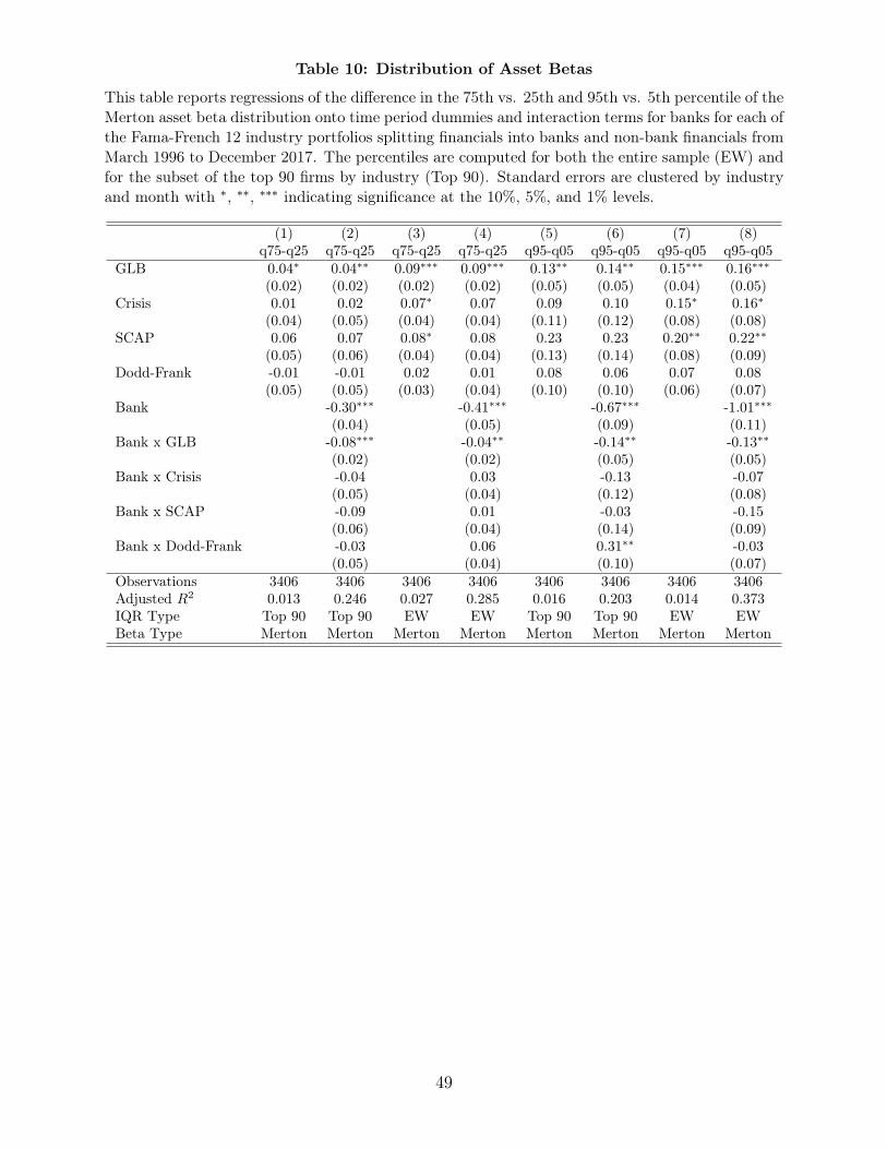
Table 10: Distribution of Asset Betas

This table reports regressions of the difference in the 75th vs. 25th and 95th vs. 5th percentile of theMerton asset beta distribution onto time period dummies and interaction terms for banks for each ofthe Fama-French 12 industry portfolios splitting financials into banks and non-bank financials fromMarch 1996 to December 2017. The percentiles are computed for both the entire sample (EW) andfor the subset of the top 90 firms by industry (Top 90). Standard errors are clustered by industryand month with ∗, ∗∗, ∗∗∗ indicating significance at the 10%, 5%, and 1% levels.

(1) (2) (3) (4) (5) (6) (7) (8)q75-q25 q75-q25 q75-q25 q75-q25 q95-q05 q95-q05 q95-q05 q95-q05

GLB 0.04∗ 0.04∗∗ 0.09∗∗∗ 0.09∗∗∗ 0.13∗∗ 0.14∗∗ 0.15∗∗∗ 0.16∗∗∗(0.02) (0.02) (0.02) (0.02) (0.05) (0.05) (0.04) (0.05)

Crisis 0.01 0.02 0.07∗ 0.07 0.09 0.10 0.15∗ 0.16∗(0.04) (0.05) (0.04) (0.04) (0.11) (0.12) (0.08) (0.08)

SCAP 0.06 0.07 0.08∗ 0.08 0.23 0.23 0.20∗∗ 0.22∗∗(0.05) (0.06) (0.04) (0.04) (0.13) (0.14) (0.08) (0.09)

Dodd-Frank -0.01 -0.01 0.02 0.01 0.08 0.06 0.07 0.08(0.05) (0.05) (0.03) (0.04) (0.10) (0.10) (0.06) (0.07)

Bank -0.30∗∗∗ -0.41∗∗∗ -0.67∗∗∗ -1.01∗∗∗(0.04) (0.05) (0.09) (0.11)

Bank x GLB -0.08∗∗∗ -0.04∗∗ -0.14∗∗ -0.13∗∗(0.02) (0.02) (0.05) (0.05)

Bank x Crisis -0.04 0.03 -0.13 -0.07(0.05) (0.04) (0.12) (0.08)

Bank x SCAP -0.09 0.01 -0.03 -0.15(0.06) (0.04) (0.14) (0.09)

Bank x Dodd-Frank -0.03 0.06 0.31∗∗ -0.03(0.05) (0.04) (0.10) (0.07)

Observations 3406 3406 3406 3406 3406 3406 3406 3406Adjusted R2 0.013 0.246 0.027 0.285 0.016 0.203 0.014 0.373IQR Type Top 90 Top 90 EW EW Top 90 Top 90 EW EWBeta Type Merton Merton Merton Merton Merton Merton Merton Merton

49

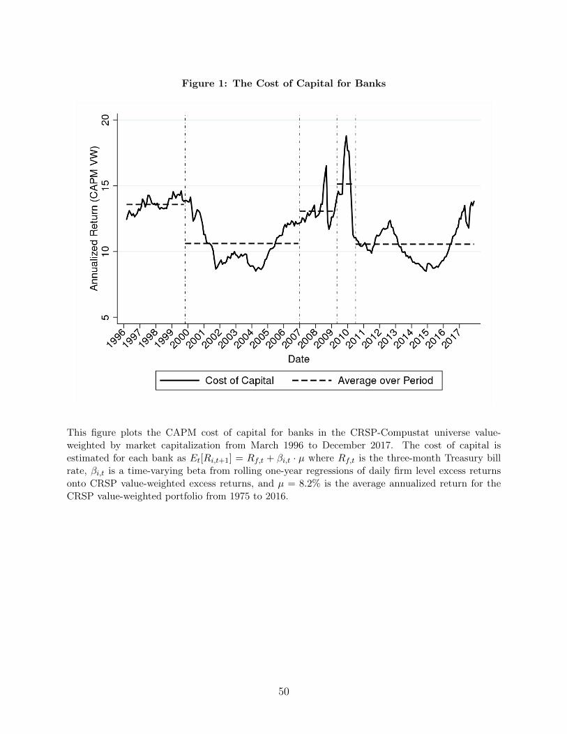
Figure 1: The Cost of Capital for Banks

This figure plots the CAPM cost of capital for banks in the CRSP-Compustat universe value-weighted by market capitalization from March 1996 to December 2017. The cost of capital isestimated for each bank as Et[Ri,t+1] = Rf,t + βi,t · µ where Rf,t is the three-month Treasury billrate, βi,t is a time-varying beta from rolling one-year regressions of daily firm level excess returnsonto CRSP value-weighted excess returns, and µ = 8.2% is the average annualized return for theCRSP value-weighted portfolio from 1975 to 2016.

50

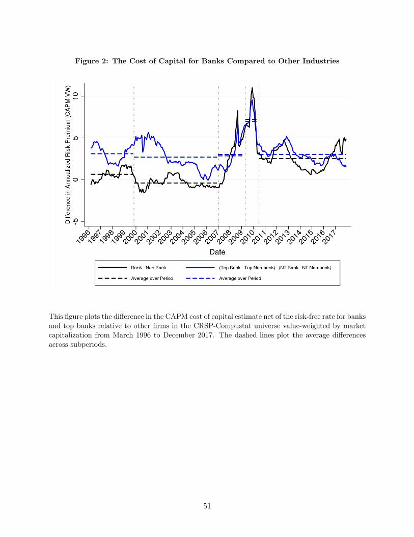
Figure 2: The Cost of Capital for Banks Compared to Other Industries

This figure plots the difference in the CAPM cost of capital estimate net of the risk-free rate for banksand top banks relative to other firms in the CRSP-Compustat universe value-weighted by marketcapitalization from March 1996 to December 2017. The dashed lines plot the average differencesacross subperiods.

51

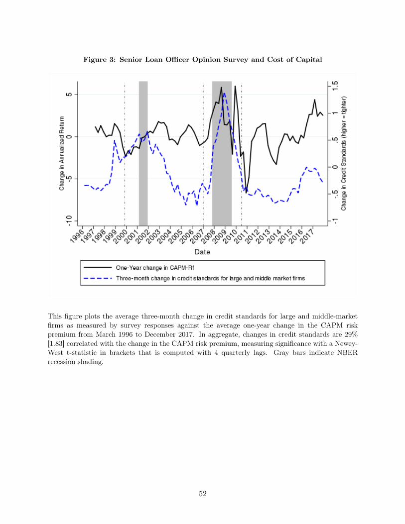
Figure 3: Senior Loan Officer Opinion Survey and Cost of Capital

This figure plots the average three-month change in credit standards for large and middle-marketfirms as measured by survey responses against the average one-year change in the CAPM riskpremium from March 1996 to December 2017. In aggregate, changes in credit standards are 29%[1.83] correlated with the change in the CAPM risk premium, measuring significance with a Newey-West t-statistic in brackets that is computed with 4 quarterly lags. Gray bars indicate NBERrecession shading.

52

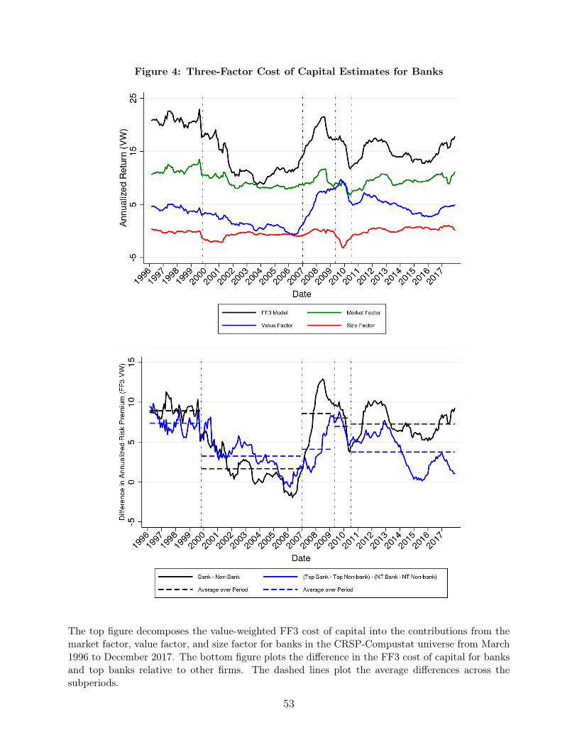
Figure 4: Three-Factor Cost of Capital Estimates for Banks

The top figure decomposes the value-weighted FF3 cost of capital into the contributions from themarket factor, value factor, and size factor for banks in the CRSP-Compustat universe from March1996 to December 2017. The bottom figure plots the difference in the FF3 cost of capital for banksand top banks relative to other firms. The dashed lines plot the average differences across thesubperiods.

53

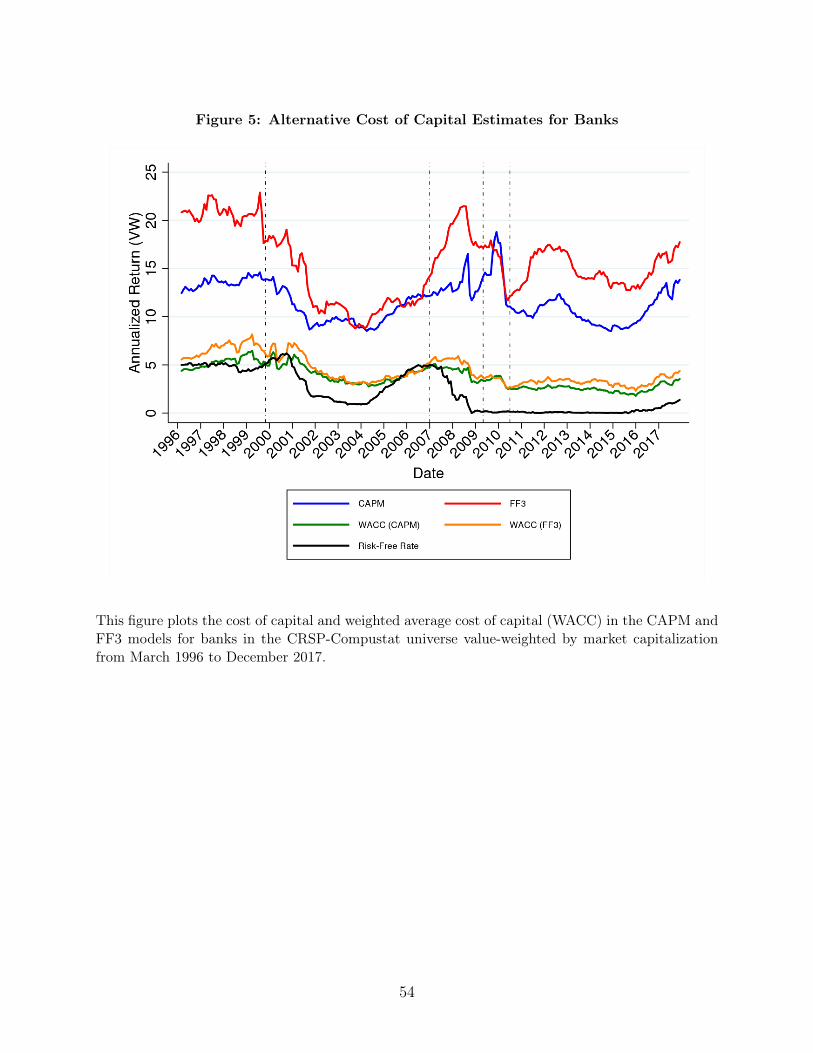
Figure 5: Alternative Cost of Capital Estimates for Banks

This figure plots the cost of capital and weighted average cost of capital (WACC) in the CAPM andFF3 models for banks in the CRSP-Compustat universe value-weighted by market capitalizationfrom March 1996 to December 2017.

54

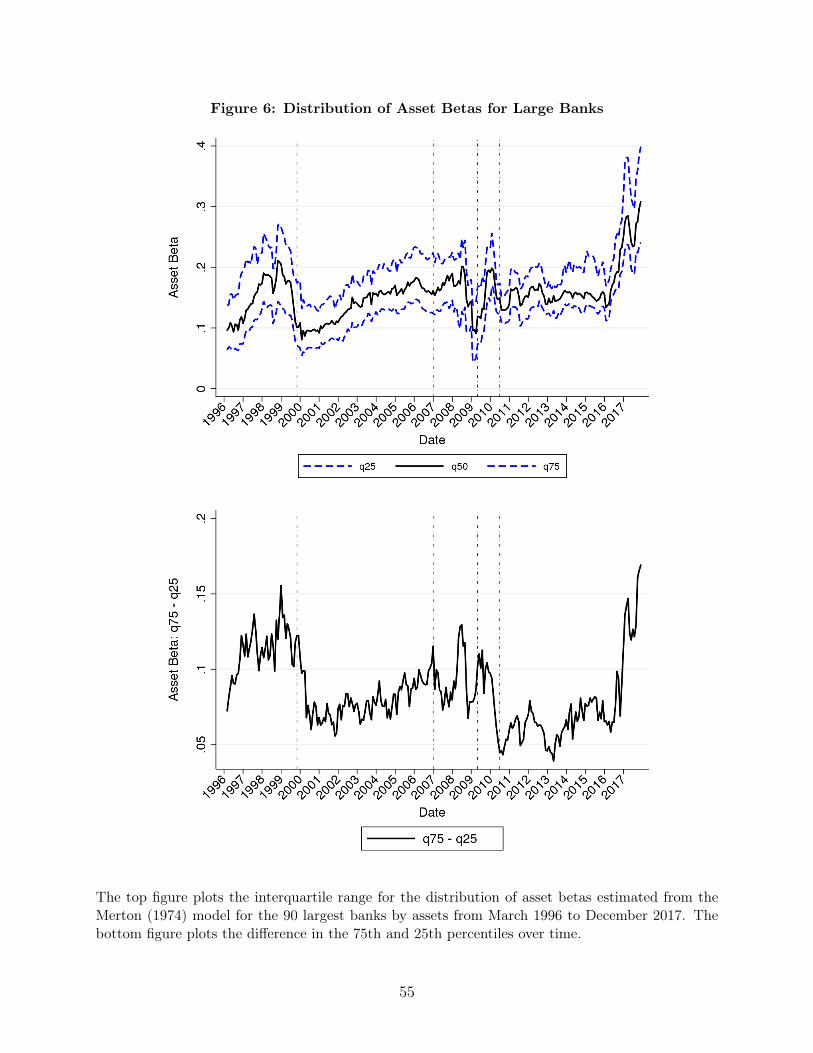
Figure 6: Distribution of Asset Betas for Large Banks

The top figure plots the interquartile range for the distribution of asset betas estimated from theMerton (1974) model for the 90 largest banks by assets from March 1996 to December 2017. Thebottom figure plots the difference in the 75th and 25th percentiles over time.

55

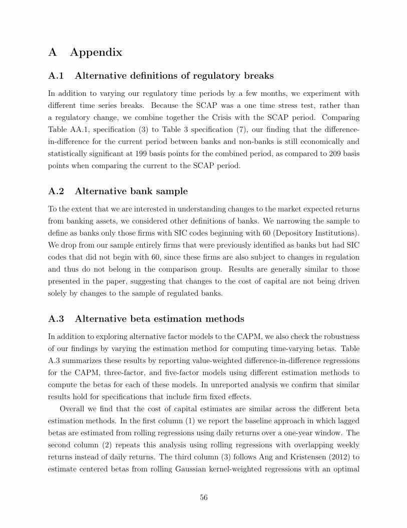
A Appendix

A.1 Alternative definitions of regulatory breaks

In addition to varying our regulatory time periods by a few months, we experiment withdifferent time series breaks. Because the SCAP was a one time stress test, rather thana regulatory change, we combine together the Crisis with the SCAP period. ComparingTable AA.1, specification (3) to Table 3 specification (7), our finding that the difference-in-difference for the current period between banks and non-banks is still economically andstatistically significant at 199 basis points for the combined period, as compared to 209 basispoints when comparing the current to the SCAP period.

A.2 Alternative bank sample

To the extent that we are interested in understanding changes to the market expected returnsfrom banking assets, we considered other definitions of banks. We narrowing the sample todefine as banks only those firms with SIC codes beginning with 60 (Depository Institutions).We drop from our sample entirely firms that were previously identified as banks but had SICcodes that did not begin with 60, since these firms are also subject to changes in regulationand thus do not belong in the comparison group. Results are generally similar to thosepresented in the paper, suggesting that changes to the cost of capital are not being drivensolely by changes to the sample of regulated banks.

A.3 Alternative beta estimation methods

In addition to exploring alternative factor models to the CAPM, we also check the robustnessof our findings by varying the estimation method for computing time-varying betas. TableA.3 summarizes these results by reporting value-weighted difference-in-difference regressionsfor the CAPM, three-factor, and five-factor models using different estimation methods tocompute the betas for each of these models. In unreported analysis we confirm that similarresults hold for specifications that include firm fixed effects.

Overall we find that the cost of capital estimates are similar across the different betaestimation methods. In the first column (1) we report the baseline approach in which laggedbetas are estimated from rolling regressions using daily returns over a one-year window. Thesecond column (2) repeats this analysis using rolling regressions with overlapping weeklyreturns instead of daily returns. The third column (3) follows Ang and Kristensen (2012) toestimate centered betas from rolling Gaussian kernel-weighted regressions with an optimal

56

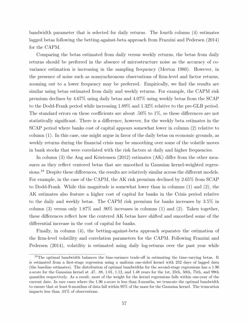
bandwidth parameter that is selected for daily returns. The fourth column (4) estimateslagged betas following the betting-against-beta approach from Frazzini and Pedersen (2014)for the CAPM.

Comparing the betas estimated from daily versus weekly returns, the betas from dailyreturns should be preferred in the absence of microstructure noise as the accuracy of co-variance estimation is increasing in the sampling frequency (Merton 1980). However, inthe presence of noise such as nonsynchronous observations of firm-level and factor returns,zooming out to a lower frequency may be preferred. Empirically, we find the results aresimilar using betas estimated from daily and weekly returns. For example, the CAPM riskpremium declines by 4.67% using daily betas and 4.07% using weekly betas from the SCAPto the Dodd-Frank period while increasing 1.89% and 1.32% relative to the pre-GLB period.The standard errors on these coefficients are about .50% to 1%, so these differences are notstatistically significant. There is a difference, however, for the weekly beta estimates in theSCAP period where banks cost of capital appears somewhat lower in column (2) relative tocolumn (1). In this case, one might argue in favor of the daily betas on economic grounds, asweekly returns during the financial crisis may be smoothing over some of the volatile movesin bank stocks that were correlated with the risk factors at daily and higher frequencies.

In column (3) the Ang and Kristensen (2012) estimates (AK) differ from the other mea-sures as they reflect centered betas that are smoothed in Gaussian kernel-weighted regres-sions.19 Despite these differences, the results are relatively similar across the different models.For example, in the case of the CAPM, the AK risk premium declined by 2.65% from SCAPto Dodd-Frank. While this magnitude is somewhat lower than in columns (1) and (2), theAK estimates also feature a higher cost of capital for banks in the Crisis period relativeto the daily and weekly betas. The CAPM risk premium for banks increases by 3.5% incolumn (3) versus only 1.87% and .90% increases in columns (1) and (2). Taken together,these differences reflect how the centered AK betas have shifted and smoothed some of thedifferential increase in the cost of capital for banks.

Finally, in column (4), the betting-against-beta approach separates the estimation ofthe firm-level volatility and correlation parameters for the CAPM. Following Frazzini andPedersen (2014), volatility is estimated using daily log-returns over the past year while

19The optimal bandwidth balances the bias-variance trade-off in estimating the time-varying betas. Itis estimated from a first-stage regression using a uniform one-sided kernel with 252 days of lagged data(the baseline estimates). The distribution of optimal bandwidths for the second-stage regressions has a 1.96z-score for the Gaussian kernel at .47, .88, 1.01, 1.12, and 1.48 years for the 1st, 25th, 50th, 75th, and 99thquantiles respectively. As a result, most of the weight for the kernel regressions falls within one-year of thecurrent date. In rare cases where the 1.96 z-score is less than 3-months, we truncate the optimal bandwidthto ensure that at least 6-monthns of data fall within 95% of the mass for the Gaussian kernel. The truncationimpacts less than .01% of observations.

57

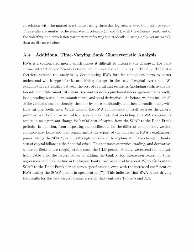
correlation with the market is estimated using three-day log returns over the past five years.The results are similar to the estimates in columns (1) and (2), with the different treatment ofthe volatility and correlation parameters reflecting the tradeoffs in using daily versus weeklydata as discussed above.

A.4 Additional Time-Varying Bank Characteristic Analysis

RWA is a complicated metric which makes it difficult to interpret the change in the bankx time interaction coefficients between column (2) and column (7) in Table 5. Table A.4therefore extends the analysis by decomposing RWA into its component parts to betterunderstand which type of risks are driving changes in the cost of capital over time. Weexamine the relationship between the cost of capital and securities (including cash, available-for-sale and held-to-maturity securities, and securities purchased under agreements to resell),loans, trading assets, loan commitments, and total derivatives. As before, we first include allof the variables unconditionally, then one by one conditionally, and then all conditionally withtime-varying coefficients. While none of the RWA components by itself reverses the generalpatterns, we do find, as in Table 5 specification (7), that including all RWA componentsresults in no significant change for banks’ cost of capital from the SCAP to the Dodd-Frankperiods. In addition, from inspecting the coefficients for the different components, we findevidence that loans and loan commitments drive part of the increase in RWA’s explanatorypower during the SCAP period, although not enough to explain all of the change in banks’cost of capital following the financial crisis. This contrasts securities, trading, and derivativeswhose coefficients are roughly stable since the GLB period. Finally, we extend the analysisfrom Table 5 for the largest banks by adding the bank x Top interaction terms. In theseregressions we find a decline in the largest banks’ cost of capital by about 3% to 4% from theSCAP to the Dodd-Frank period across specifications, even with the increased coefficient onRWA during the SCAP period in specification (7). This indicates that RWA is not drivingthe results for the very largest banks, a result that contrasts Tables 5 and A.4.

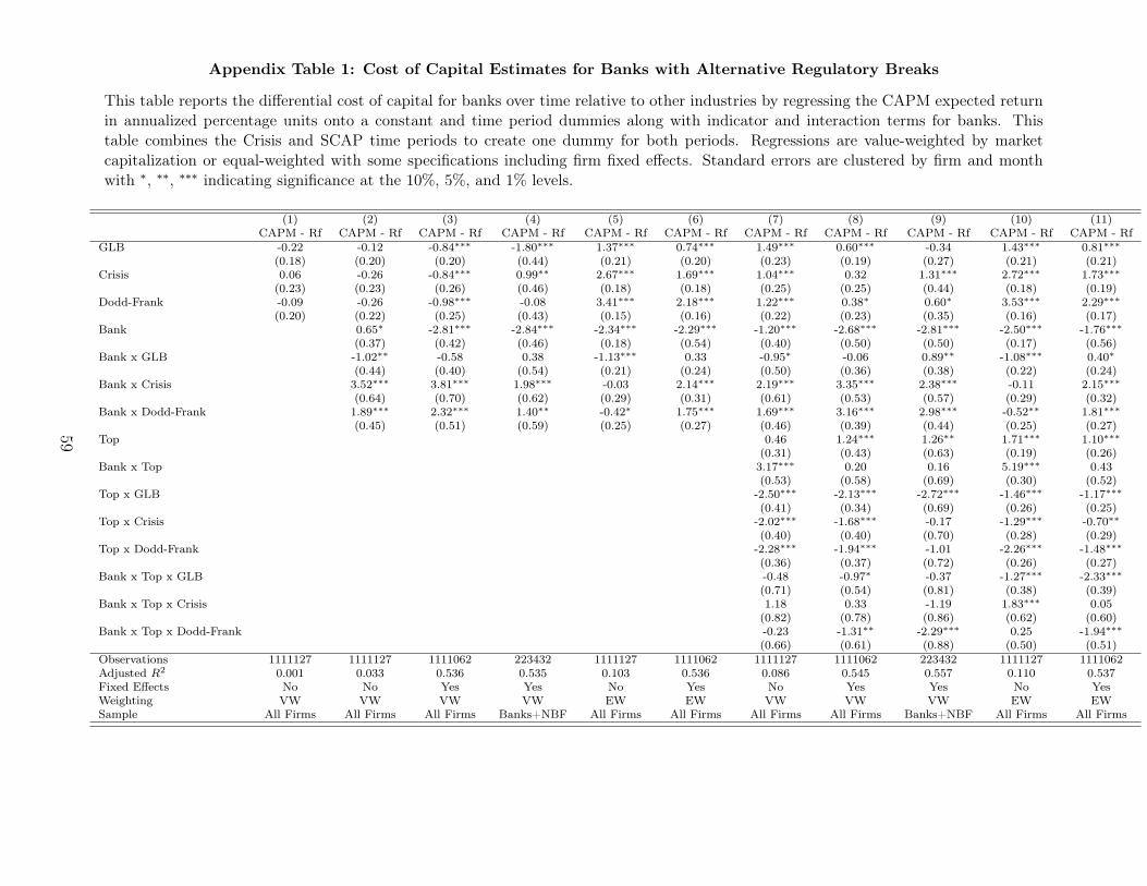
Appendix Table 1: Cost of Capital Estimates for Banks with Alternative Regulatory Breaks

This table reports the differential cost of capital for banks over time relative to other industries by regressing the CAPM expected returnin annualized percentage units onto a constant and time period dummies along with indicator and interaction terms for banks. Thistable combines the Crisis and SCAP time periods to create one dummy for both periods. Regressions are value-weighted by marketcapitalization or equal-weighted with some specifications including firm fixed effects. Standard errors are clustered by firm and monthwith ∗, ∗∗, ∗∗∗ indicating significance at the 10%, 5%, and 1% levels.

(1) (2) (3) (4) (5) (6) (7) (8) (9) (10) (11)CAPM - Rf CAPM - Rf CAPM - Rf CAPM - Rf CAPM - Rf CAPM - Rf CAPM - Rf CAPM - Rf CAPM - Rf CAPM - Rf CAPM - Rf

GLB -0.22 -0.12 -0.84∗∗∗ -1.80∗∗∗ 1.37∗∗∗ 0.74∗∗∗ 1.49∗∗∗ 0.60∗∗∗ -0.34 1.43∗∗∗ 0.81∗∗∗(0.18) (0.20) (0.20) (0.44) (0.21) (0.20) (0.23) (0.19) (0.27) (0.21) (0.21)

Crisis 0.06 -0.26 -0.84∗∗∗ 0.99∗∗ 2.67∗∗∗ 1.69∗∗∗ 1.04∗∗∗ 0.32 1.31∗∗∗ 2.72∗∗∗ 1.73∗∗∗(0.23) (0.23) (0.26) (0.46) (0.18) (0.18) (0.25) (0.25) (0.44) (0.18) (0.19)

Dodd-Frank -0.09 -0.26 -0.98∗∗∗ -0.08 3.41∗∗∗ 2.18∗∗∗ 1.22∗∗∗ 0.38∗ 0.60∗ 3.53∗∗∗ 2.29∗∗∗(0.20) (0.22) (0.25) (0.43) (0.15) (0.16) (0.22) (0.23) (0.35) (0.16) (0.17)

Bank 0.65∗ -2.81∗∗∗ -2.84∗∗∗ -2.34∗∗∗ -2.29∗∗∗ -1.20∗∗∗ -2.68∗∗∗ -2.81∗∗∗ -2.50∗∗∗ -1.76∗∗∗(0.37) (0.42) (0.46) (0.18) (0.54) (0.40) (0.50) (0.50) (0.17) (0.56)

Bank x GLB -1.02∗∗ -0.58 0.38 -1.13∗∗∗ 0.33 -0.95∗ -0.06 0.89∗∗ -1.08∗∗∗ 0.40∗(0.44) (0.40) (0.54) (0.21) (0.24) (0.50) (0.36) (0.38) (0.22) (0.24)

Bank x Crisis 3.52∗∗∗ 3.81∗∗∗ 1.98∗∗∗ -0.03 2.14∗∗∗ 2.19∗∗∗ 3.35∗∗∗ 2.38∗∗∗ -0.11 2.15∗∗∗(0.64) (0.70) (0.62) (0.29) (0.31) (0.61) (0.53) (0.57) (0.29) (0.32)

Bank x Dodd-Frank 1.89∗∗∗ 2.32∗∗∗ 1.40∗∗ -0.42∗ 1.75∗∗∗ 1.69∗∗∗ 3.16∗∗∗ 2.98∗∗∗ -0.52∗∗ 1.81∗∗∗(0.45) (0.51) (0.59) (0.25) (0.27) (0.46) (0.39) (0.44) (0.25) (0.27)

Top 0.46 1.24∗∗∗ 1.26∗∗ 1.71∗∗∗ 1.10∗∗∗(0.31) (0.43) (0.63) (0.19) (0.26)

Bank x Top 3.17∗∗∗ 0.20 0.16 5.19∗∗∗ 0.43(0.53) (0.58) (0.69) (0.30) (0.52)

Top x GLB -2.50∗∗∗ -2.13∗∗∗ -2.72∗∗∗ -1.46∗∗∗ -1.17∗∗∗(0.41) (0.34) (0.69) (0.26) (0.25)

Top x Crisis -2.02∗∗∗ -1.68∗∗∗ -0.17 -1.29∗∗∗ -0.70∗∗(0.40) (0.40) (0.70) (0.28) (0.29)

Top x Dodd-Frank -2.28∗∗∗ -1.94∗∗∗ -1.01 -2.26∗∗∗ -1.48∗∗∗(0.36) (0.37) (0.72) (0.26) (0.27)

Bank x Top x GLB -0.48 -0.97∗ -0.37 -1.27∗∗∗ -2.33∗∗∗(0.71) (0.54) (0.81) (0.38) (0.39)

Bank x Top x Crisis 1.18 0.33 -1.19 1.83∗∗∗ 0.05(0.82) (0.78) (0.86) (0.62) (0.60)

Bank x Top x Dodd-Frank -0.23 -1.31∗∗ -2.29∗∗∗ 0.25 -1.94∗∗∗(0.66) (0.61) (0.88) (0.50) (0.51)

Observations 1111127 1111127 1111062 223432 1111127 1111062 1111127 1111062 223432 1111127 1111062Adjusted R2 0.001 0.033 0.536 0.535 0.103 0.536 0.086 0.545 0.557 0.110 0.537Fixed Effects No No Yes Yes No Yes No Yes Yes No YesWeighting VW VW VW VW EW EW VW VW VW EW EWSample All Firms All Firms All Firms Banks+NBF All Firms All Firms All Firms All Firms Banks+NBF All Firms All Firms

59

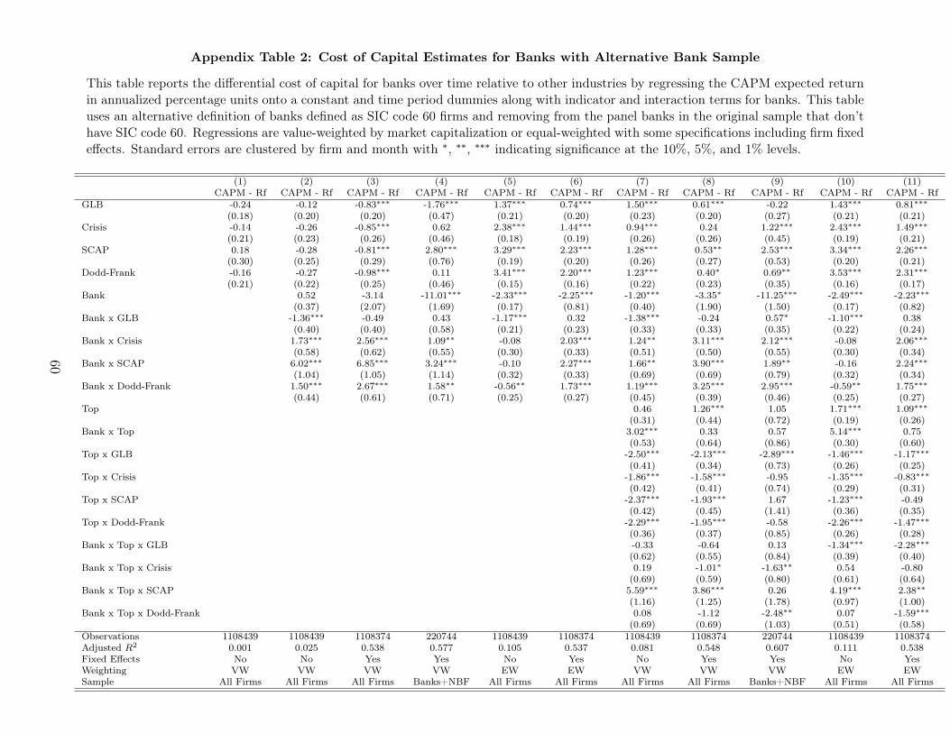
Appendix Table 2: Cost of Capital Estimates for Banks with Alternative Bank Sample

This table reports the differential cost of capital for banks over time relative to other industries by regressing the CAPM expected returnin annualized percentage units onto a constant and time period dummies along with indicator and interaction terms for banks. This tableuses an alternative definition of banks defined as SIC code 60 firms and removing from the panel banks in the original sample that don’thave SIC code 60. Regressions are value-weighted by market capitalization or equal-weighted with some specifications including firm fixedeffects. Standard errors are clustered by firm and month with ∗, ∗∗, ∗∗∗ indicating significance at the 10%, 5%, and 1% levels.

(1) (2) (3) (4) (5) (6) (7) (8) (9) (10) (11)CAPM - Rf CAPM - Rf CAPM - Rf CAPM - Rf CAPM - Rf CAPM - Rf CAPM - Rf CAPM - Rf CAPM - Rf CAPM - Rf CAPM - Rf

GLB -0.24 -0.12 -0.83∗∗∗ -1.76∗∗∗ 1.37∗∗∗ 0.74∗∗∗ 1.50∗∗∗ 0.61∗∗∗ -0.22 1.43∗∗∗ 0.81∗∗∗(0.18) (0.20) (0.20) (0.47) (0.21) (0.20) (0.23) (0.20) (0.27) (0.21) (0.21)

Crisis -0.14 -0.26 -0.85∗∗∗ 0.62 2.38∗∗∗ 1.44∗∗∗ 0.94∗∗∗ 0.24 1.22∗∗∗ 2.43∗∗∗ 1.49∗∗∗(0.21) (0.23) (0.26) (0.46) (0.18) (0.19) (0.26) (0.26) (0.45) (0.19) (0.21)

SCAP 0.18 -0.28 -0.81∗∗∗ 2.80∗∗∗ 3.29∗∗∗ 2.23∗∗∗ 1.28∗∗∗ 0.53∗∗ 2.53∗∗∗ 3.34∗∗∗ 2.26∗∗∗(0.30) (0.25) (0.29) (0.76) (0.19) (0.20) (0.26) (0.27) (0.53) (0.20) (0.21)

Dodd-Frank -0.16 -0.27 -0.98∗∗∗ 0.11 3.41∗∗∗ 2.20∗∗∗ 1.23∗∗∗ 0.40∗ 0.69∗∗ 3.53∗∗∗ 2.31∗∗∗(0.21) (0.22) (0.25) (0.46) (0.15) (0.16) (0.22) (0.23) (0.35) (0.16) (0.17)

Bank 0.52 -3.14 -11.01∗∗∗ -2.33∗∗∗ -2.25∗∗∗ -1.20∗∗∗ -3.35∗ -11.25∗∗∗ -2.49∗∗∗ -2.23∗∗∗(0.37) (2.07) (1.69) (0.17) (0.81) (0.40) (1.90) (1.50) (0.17) (0.82)

Bank x GLB -1.36∗∗∗ -0.49 0.43 -1.17∗∗∗ 0.32 -1.38∗∗∗ -0.24 0.57∗ -1.10∗∗∗ 0.38(0.40) (0.40) (0.58) (0.21) (0.23) (0.33) (0.33) (0.35) (0.22) (0.24)

Bank x Crisis 1.73∗∗∗ 2.56∗∗∗ 1.09∗∗ -0.08 2.03∗∗∗ 1.24∗∗ 3.11∗∗∗ 2.12∗∗∗ -0.08 2.06∗∗∗(0.58) (0.62) (0.55) (0.30) (0.33) (0.51) (0.50) (0.55) (0.30) (0.34)

Bank x SCAP 6.02∗∗∗ 6.85∗∗∗ 3.24∗∗∗ -0.10 2.27∗∗∗ 1.66∗∗ 3.90∗∗∗ 1.89∗∗ -0.16 2.24∗∗∗(1.04) (1.05) (1.14) (0.32) (0.33) (0.69) (0.69) (0.79) (0.32) (0.34)

Bank x Dodd-Frank 1.50∗∗∗ 2.67∗∗∗ 1.58∗∗ -0.56∗∗ 1.73∗∗∗ 1.19∗∗∗ 3.25∗∗∗ 2.95∗∗∗ -0.59∗∗ 1.75∗∗∗(0.44) (0.61) (0.71) (0.25) (0.27) (0.45) (0.39) (0.46) (0.25) (0.27)

Top 0.46 1.26∗∗∗ 1.05 1.71∗∗∗ 1.09∗∗∗(0.31) (0.44) (0.72) (0.19) (0.26)

Bank x Top 3.02∗∗∗ 0.33 0.57 5.14∗∗∗ 0.75(0.53) (0.64) (0.86) (0.30) (0.60)

Top x GLB -2.50∗∗∗ -2.13∗∗∗ -2.89∗∗∗ -1.46∗∗∗ -1.17∗∗∗(0.41) (0.34) (0.73) (0.26) (0.25)

Top x Crisis -1.86∗∗∗ -1.58∗∗∗ -0.95 -1.35∗∗∗ -0.83∗∗∗(0.42) (0.41) (0.74) (0.29) (0.31)

Top x SCAP -2.37∗∗∗ -1.93∗∗∗ 1.67 -1.23∗∗∗ -0.49(0.42) (0.45) (1.41) (0.36) (0.35)

Top x Dodd-Frank -2.29∗∗∗ -1.95∗∗∗ -0.58 -2.26∗∗∗ -1.47∗∗∗(0.36) (0.37) (0.85) (0.26) (0.28)

Bank x Top x GLB -0.33 -0.64 0.13 -1.34∗∗∗ -2.28∗∗∗(0.62) (0.55) (0.84) (0.39) (0.40)

Bank x Top x Crisis 0.19 -1.01∗ -1.63∗∗ 0.54 -0.80(0.69) (0.59) (0.80) (0.61) (0.64)

Bank x Top x SCAP 5.59∗∗∗ 3.86∗∗∗ 0.26 4.19∗∗∗ 2.38∗∗(1.16) (1.25) (1.78) (0.97) (1.00)

Bank x Top x Dodd-Frank 0.08 -1.12 -2.48∗∗ 0.07 -1.59∗∗∗(0.69) (0.69) (1.03) (0.51) (0.58)

Observations 1108439 1108439 1108374 220744 1108439 1108374 1108439 1108374 220744 1108439 1108374Adjusted R2 0.001 0.025 0.538 0.577 0.105 0.537 0.081 0.548 0.607 0.111 0.538Fixed Effects No No Yes Yes No Yes No Yes Yes No YesWeighting VW VW VW VW EW EW VW VW VW EW EWSample All Firms All Firms All Firms Banks+NBF All Firms All Firms All Firms All Firms Banks+NBF All Firms All Firms

60

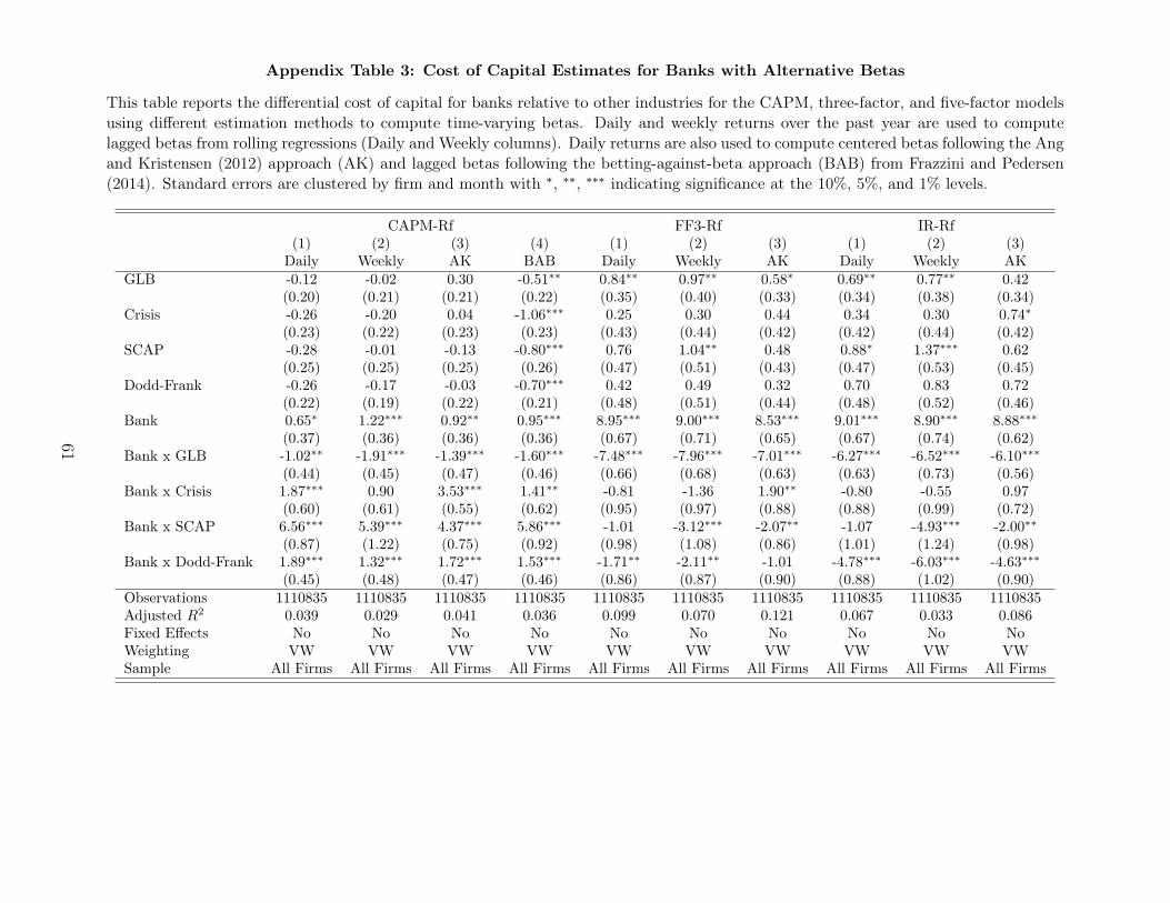
Appendix Table 3: Cost of Capital Estimates for Banks with Alternative Betas

This table reports the differential cost of capital for banks relative to other industries for the CAPM, three-factor, and five-factor modelsusing different estimation methods to compute time-varying betas. Daily and weekly returns over the past year are used to computelagged betas from rolling regressions (Daily and Weekly columns). Daily returns are also used to compute centered betas following the Angand Kristensen (2012) approach (AK) and lagged betas following the betting-against-beta approach (BAB) from Frazzini and Pedersen(2014). Standard errors are clustered by firm and month with ∗, ∗∗, ∗∗∗ indicating significance at the 10%, 5%, and 1% levels.

CAPM-Rf FF3-Rf IR-Rf(1) (2) (3) (4) (1) (2) (3) (1) (2) (3)

Daily Weekly AK BAB Daily Weekly AK Daily Weekly AKGLB -0.12 -0.02 0.30 -0.51∗∗ 0.84∗∗ 0.97∗∗ 0.58∗ 0.69∗∗ 0.77∗∗ 0.42

(0.20) (0.21) (0.21) (0.22) (0.35) (0.40) (0.33) (0.34) (0.38) (0.34)Crisis -0.26 -0.20 0.04 -1.06∗∗∗ 0.25 0.30 0.44 0.34 0.30 0.74∗

(0.23) (0.22) (0.23) (0.23) (0.43) (0.44) (0.42) (0.42) (0.44) (0.42)SCAP -0.28 -0.01 -0.13 -0.80∗∗∗ 0.76 1.04∗∗ 0.48 0.88∗ 1.37∗∗∗ 0.62

(0.25) (0.25) (0.25) (0.26) (0.47) (0.51) (0.43) (0.47) (0.53) (0.45)Dodd-Frank -0.26 -0.17 -0.03 -0.70∗∗∗ 0.42 0.49 0.32 0.70 0.83 0.72

(0.22) (0.19) (0.22) (0.21) (0.48) (0.51) (0.44) (0.48) (0.52) (0.46)Bank 0.65∗ 1.22∗∗∗ 0.92∗∗ 0.95∗∗∗ 8.95∗∗∗ 9.00∗∗∗ 8.53∗∗∗ 9.01∗∗∗ 8.90∗∗∗ 8.88∗∗∗

(0.37) (0.36) (0.36) (0.36) (0.67) (0.71) (0.65) (0.67) (0.74) (0.62)Bank x GLB -1.02∗∗ -1.91∗∗∗ -1.39∗∗∗ -1.60∗∗∗ -7.48∗∗∗ -7.96∗∗∗ -7.01∗∗∗ -6.27∗∗∗ -6.52∗∗∗ -6.10∗∗∗

(0.44) (0.45) (0.47) (0.46) (0.66) (0.68) (0.63) (0.63) (0.73) (0.56)Bank x Crisis 1.87∗∗∗ 0.90 3.53∗∗∗ 1.41∗∗ -0.81 -1.36 1.90∗∗ -0.80 -0.55 0.97

(0.60) (0.61) (0.55) (0.62) (0.95) (0.97) (0.88) (0.88) (0.99) (0.72)Bank x SCAP 6.56∗∗∗ 5.39∗∗∗ 4.37∗∗∗ 5.86∗∗∗ -1.01 -3.12∗∗∗ -2.07∗∗ -1.07 -4.93∗∗∗ -2.00∗∗

(0.87) (1.22) (0.75) (0.92) (0.98) (1.08) (0.86) (1.01) (1.24) (0.98)Bank x Dodd-Frank 1.89∗∗∗ 1.32∗∗∗ 1.72∗∗∗ 1.53∗∗∗ -1.71∗∗ -2.11∗∗ -1.01 -4.78∗∗∗ -6.03∗∗∗ -4.63∗∗∗

(0.45) (0.48) (0.47) (0.46) (0.86) (0.87) (0.90) (0.88) (1.02) (0.90)Observations 1110835 1110835 1110835 1110835 1110835 1110835 1110835 1110835 1110835 1110835Adjusted R2 0.039 0.029 0.041 0.036 0.099 0.070 0.121 0.067 0.033 0.086Fixed Effects No No No No No No No No No NoWeighting VW VW VW VW VW VW VW VW VW VWSample All Firms All Firms All Firms All Firms All Firms All Firms All Firms All Firms All Firms All Firms

61

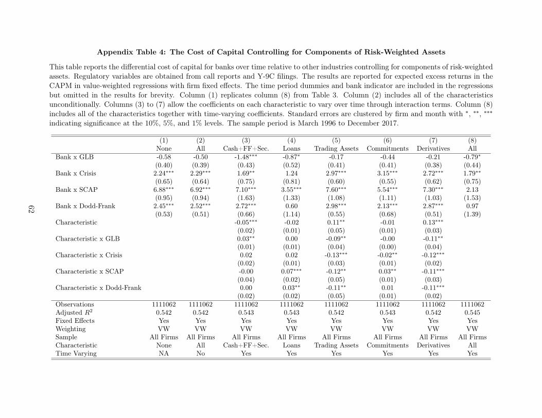
Appendix Table 4: The Cost of Capital Controlling for Components of Risk-Weighted Assets

This table reports the differential cost of capital for banks over time relative to other industries controlling for components of risk-weightedassets. Regulatory variables are obtained from call reports and Y-9C filings. The results are reported for expected excess returns in theCAPM in value-weighted regressions with firm fixed effects. The time period dummies and bank indicator are included in the regressionsbut omitted in the results for brevity. Column (1) replicates column (8) from Table 3. Column (2) includes all of the characteristicsunconditionally. Columns (3) to (7) allow the coefficients on each characteristic to vary over time through interaction terms. Column (8)includes all of the characteristics together with time-varying coefficients. Standard errors are clustered by firm and month with ∗, ∗∗, ∗∗∗

indicating significance at the 10%, 5%, and 1% levels. The sample period is March 1996 to December 2017.

(1) (2) (3) (4) (5) (6) (7) (8)None All Cash+FF+Sec. Loans Trading Assets Commitments Derivatives All

Bank x GLB -0.58 -0.50 -1.48∗∗∗ -0.87∗ -0.17 -0.44 -0.21 -0.79∗(0.40) (0.39) (0.43) (0.52) (0.41) (0.41) (0.38) (0.44)

Bank x Crisis 2.24∗∗∗ 2.29∗∗∗ 1.69∗∗ 1.24 2.97∗∗∗ 3.15∗∗∗ 2.72∗∗∗ 1.79∗∗(0.65) (0.64) (0.75) (0.81) (0.60) (0.55) (0.62) (0.75)

Bank x SCAP 6.88∗∗∗ 6.92∗∗∗ 7.10∗∗∗ 3.55∗∗∗ 7.60∗∗∗ 5.54∗∗∗ 7.30∗∗∗ 2.13(0.95) (0.94) (1.63) (1.33) (1.08) (1.11) (1.03) (1.53)

Bank x Dodd-Frank 2.45∗∗∗ 2.52∗∗∗ 2.72∗∗∗ 0.60 2.98∗∗∗ 2.13∗∗∗ 2.87∗∗∗ 0.97(0.53) (0.51) (0.66) (1.14) (0.55) (0.68) (0.51) (1.39)

Characteristic -0.05∗∗∗ -0.02 0.11∗∗ -0.01 0.13∗∗∗(0.02) (0.01) (0.05) (0.01) (0.03)

Characteristic x GLB 0.03∗∗ 0.00 -0.09∗∗ -0.00 -0.11∗∗(0.01) (0.01) (0.04) (0.00) (0.04)

Characteristic x Crisis 0.02 0.02 -0.13∗∗∗ -0.02∗∗ -0.12∗∗∗(0.02) (0.01) (0.03) (0.01) (0.02)

Characteristic x SCAP -0.00 0.07∗∗∗ -0.12∗∗ 0.03∗∗ -0.11∗∗∗(0.04) (0.02) (0.05) (0.01) (0.03)

Characteristic x Dodd-Frank 0.00 0.03∗∗ -0.11∗∗ 0.01 -0.11∗∗∗(0.02) (0.02) (0.05) (0.01) (0.02)

Observations 1111062 1111062 1111062 1111062 1111062 1111062 1111062 1111062Adjusted R2 0.542 0.542 0.543 0.543 0.542 0.543 0.542 0.545Fixed Effects Yes Yes Yes Yes Yes Yes Yes YesWeighting VW VW VW VW VW VW VW VWSample All Firms All Firms All Firms All Firms All Firms All Firms All Firms All FirmsCharacteristic None All Cash+FF+Sec. Loans Trading Assets Commitments Derivatives AllTime Varying NA No Yes Yes Yes Yes Yes Yes

62

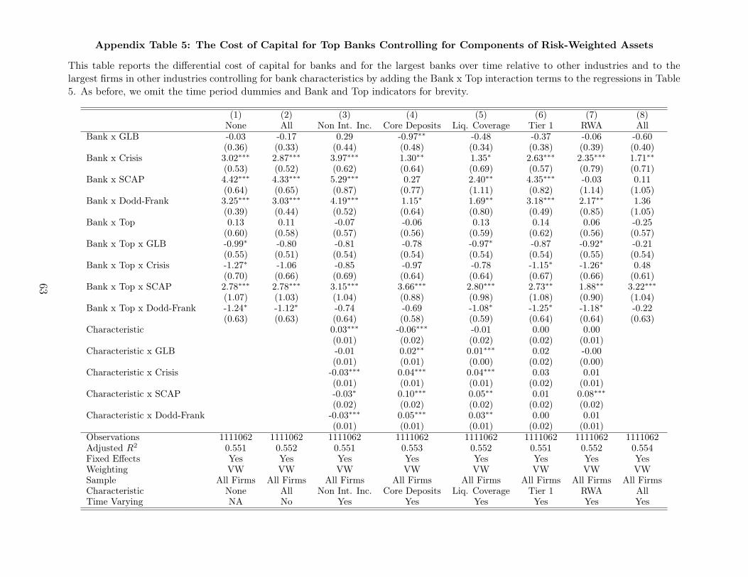
Appendix Table 5: The Cost of Capital for Top Banks Controlling for Components of Risk-Weighted Assets

This table reports the differential cost of capital for banks and for the largest banks over time relative to other industries and to thelargest firms in other industries controlling for bank characteristics by adding the Bank x Top interaction terms to the regressions in Table5. As before, we omit the time period dummies and Bank and Top indicators for brevity.

(1) (2) (3) (4) (5) (6) (7) (8)None All Non Int. Inc. Core Deposits Liq. Coverage Tier 1 RWA All

Bank x GLB -0.03 -0.17 0.29 -0.97∗∗ -0.48 -0.37 -0.06 -0.60(0.36) (0.33) (0.44) (0.48) (0.34) (0.38) (0.39) (0.40)

Bank x Crisis 3.02∗∗∗ 2.87∗∗∗ 3.97∗∗∗ 1.30∗∗ 1.35∗ 2.63∗∗∗ 2.35∗∗∗ 1.71∗∗(0.53) (0.52) (0.62) (0.64) (0.69) (0.57) (0.79) (0.71)

Bank x SCAP 4.42∗∗∗ 4.33∗∗∗ 5.29∗∗∗ 0.27 2.40∗∗ 4.35∗∗∗ -0.03 0.11(0.64) (0.65) (0.87) (0.77) (1.11) (0.82) (1.14) (1.05)

Bank x Dodd-Frank 3.25∗∗∗ 3.03∗∗∗ 4.19∗∗∗ 1.15∗ 1.69∗∗ 3.18∗∗∗ 2.17∗∗ 1.36(0.39) (0.44) (0.52) (0.64) (0.80) (0.49) (0.85) (1.05)

Bank x Top 0.13 0.11 -0.07 -0.06 0.13 0.14 0.06 -0.25(0.60) (0.58) (0.57) (0.56) (0.59) (0.62) (0.56) (0.57)

Bank x Top x GLB -0.99∗ -0.80 -0.81 -0.78 -0.97∗ -0.87 -0.92∗ -0.21(0.55) (0.51) (0.54) (0.54) (0.54) (0.54) (0.55) (0.54)

Bank x Top x Crisis -1.27∗ -1.06 -0.85 -0.97 -0.78 -1.15∗ -1.26∗ 0.48(0.70) (0.66) (0.69) (0.64) (0.64) (0.67) (0.66) (0.61)

Bank x Top x SCAP 2.78∗∗∗ 2.78∗∗∗ 3.15∗∗∗ 3.66∗∗∗ 2.80∗∗∗ 2.73∗∗ 1.88∗∗ 3.22∗∗∗(1.07) (1.03) (1.04) (0.88) (0.98) (1.08) (0.90) (1.04)

Bank x Top x Dodd-Frank -1.24∗ -1.12∗ -0.74 -0.69 -1.08∗ -1.25∗ -1.18∗ -0.22(0.63) (0.63) (0.64) (0.58) (0.59) (0.64) (0.64) (0.63)

Characteristic 0.03∗∗∗ -0.06∗∗∗ -0.01 0.00 0.00(0.01) (0.02) (0.02) (0.02) (0.01)

Characteristic x GLB -0.01 0.02∗∗ 0.01∗∗∗ 0.02 -0.00(0.01) (0.01) (0.00) (0.02) (0.00)

Characteristic x Crisis -0.03∗∗∗ 0.04∗∗∗ 0.04∗∗∗ 0.03 0.01(0.01) (0.01) (0.01) (0.02) (0.01)

Characteristic x SCAP -0.03∗ 0.10∗∗∗ 0.05∗∗ 0.01 0.08∗∗∗(0.02) (0.02) (0.02) (0.02) (0.02)

Characteristic x Dodd-Frank -0.03∗∗∗ 0.05∗∗∗ 0.03∗∗ 0.00 0.01(0.01) (0.01) (0.01) (0.02) (0.01)

Observations 1111062 1111062 1111062 1111062 1111062 1111062 1111062 1111062Adjusted R2 0.551 0.552 0.551 0.553 0.552 0.551 0.552 0.554Fixed Effects Yes Yes Yes Yes Yes Yes Yes YesWeighting VW VW VW VW VW VW VW VWSample All Firms All Firms All Firms All Firms All Firms All Firms All Firms All FirmsCharacteristic None All Non Int. Inc. Core Deposits Liq. Coverage Tier 1 RWA AllTime Varying NA No Yes Yes Yes Yes Yes Yes

63