Embed Size (px)
Citation preview

Regulated Price Plan
Price Report
November 1, 2008
to
October 31, 2009
Ontario Energy Board
October 15, 2008

RPP Price Report (Nov 08 – Oct 09)
Executive Summary i
EXECUTIVE SUMMARY
This report contains the electricity commodity prices for consumers designated by regulation under the Regulated Price Plan (RPP) for the period November 1, 2008 through October 31, 2009. The prices were developed using the methodology described in the Regulated Price Plan Manual (RPP Manual). The RPP Manual was developed within the context of a larger regulatory proceeding on the RPP involving significant stakeholder input and consultation.
The principles that have guided the Ontario Energy Board (OEB or the Board) in developing the RPP were established by the Ontario Government. In accordance with legislation, the prices paid for electricity by RPP consumers must be based on forecasts of the cost of supplying them and must be set to recover those costs. RPP prices are reviewed by the Board every six months to determine if they need to be adjusted.
In broad terms, the methodology used to develop the RPP price has two essential steps:
1. Forecasting the total RPP supply cost for the 12 months from November 1, 2008, and
2. Establishing prices to recover the forecast RPP supply cost from RPP consumers over the 12‐month period.
The calculation of the total RPP electricity supply cost involves several separate forecasts, including forecasts of:
o the hourly market price of electricity;
o the electricity consumption pattern of RPP consumers;
o the electricity supplied by those assets of Ontario Power Generation (OPG) whose price is regulated, or that are subject to a revenue limit established by the government;
o the costs related to the contracts signed by non‐utility generators (NUGs) with the former Ontario Hydro;
o the costs of the supply contracts, and conservation and demand management (CDM) initiatives of the Ontario Power Authority (OPA); and
o the net variance account balance (as of October 31, 2008) carried by the OPA.
The overall market‐based price for electricity used by RPP consumers reflects both the hourly market price of electricity and the electricity consumption pattern of RPP consumers. Residential consumers, who represent most of the RPP consumption, use relatively more of their electricity during times when total Ontario demand and prices are higher (than the overall Ontario average) and relatively less when total Ontario demand and prices are lower (than the overall Ontario average). That will make the overall market price for RPP consumers higher than the average market price for the entire Ontario electricity market.
RPP Price Report (Nov 08 – Oct 09)
Executive Summary i i
Average RPP Supply Cost
The hourly market price forecast for this computation was developed by Navigant Consulting, Inc. (Navigant Consulting or NCI). The forecast of the simple average market price for 12 months from November 1, 2008 is $50.16 / MWh (5.016 cents per kWh). After accounting for the consumption pattern of RPP consumers, the average market price for electricity used by RPP consumers is forecast to be $53.46 / MWh (5.346 cents per kWh). This represents the load‐weighted average electricity price that RPP consumers would pay if all their electricity supply was purchased out of the Ontario wholesale electricity spot market.
The combined effect of the other components of the RPP supply cost is expected to increase this price. The collective impact of the other components is summarized by two factors, the Global Adjustment (or Provincial Benefit) and the OPG Non‐prescribed asset (ONPA) rebate (or OPG Rebate).
The Global Adjustment (or Provincial Benefit) reflects the impact of the NUG contract costs, which are above market prices, the regulated prices for OPG’s prescribed baseload nuclear and hydroelectric generating facilities, which may be above or below market prices, and the cost of supply contracts held by the Ontario Power Authority (OPA), most of which are above market prices. It also reflects the cost associated with CDM initiatives implemented by the OPA. The forecast net impact of the Global Adjustment is to increase the average RPP supply cost by $8.52 / MWh (0.852 cents per kWh).
The OPG Rebate (or ONPA Rebate) reflects the revenue limit applied to OPG’s coal‐fired generating facilities and the remaining non‐prescribed hydroelectric facilities. These facilities are currently limited to $48 / MWh. This limit is scheduled to expire on April 30, 2009. The forecast net impact of the OPG Rebate is to reduce the RPP supply cost by $1.02 / MWh (0.102 cents per kWh) on average over the entire RPP period, i.e., an average of $1.83 / MWh between November 2008 and April 2009, and no impact between May and October 2009.
Another factor that needs to be taken into account is that actual prices and actual demand cannot be predicted with absolute certainty; both price and demand are subject to random effects. An additional small adjustment is therefore made to the RPP supply cost to account for the fact that these random effects are more likely to raise than to lower costs. This adjustment was determined to be $1.00 / MWh (0.100 cents per kWh). Without this adjustment, the RPP would be expected to end the year with a small debit variance.
An additional adjustment factor is required to “clear” the expected balance in the OPA variance account as of October 31, 2008. The majority of the current outstanding balance was accumulated as a result of lower than forecast electricity prices. 1 The forecast adjustment factor
1 After April 30, 2009, Municipalities, Colleges, Universities, Schools and Hospitals (the MUSH sector consumers) will no longer be eligible for supply under the RPP. As they leave the RPP, they will receive a credit of their share of the accumulated positive variance. This will contribute to clearing the variance account balance.

RPP Price Report (Nov 08 – Oct 09)
Executive Summary i i i
to clear the existing variance balance is a credit (reduction in the RPP price) of $1.66 / MWh (0.166 cents per kWh).
The resulting average RPP supply cost, or the RPA, is $60.30 / MWh (6.03 cents per kWh). This is summarized in Table ES‐1.
Table ES‐1: Average RPP Supply Cost Summary (for the 12 months from November 1, 2008)
RPP Supply Cost Summaryfor the period from November 1, 2008 through October 31, 2009
Forecast Wholesale Electricity Price $50.16Load‐Weighted Price for RPP Consumers ($ / MWh) $53.46
Impact of the Global Adjusment ($ / MWh) + $8.52Impact of the OPG Non‐prescribed Asset Rebate ($ / MWh) + ($1.02)Adjustment to Address Bias Towards Unfavourable Variance ($ / MWh) + $1.00Adjustment to Clear Existing Variance ($ / MWh) + ($1.66)
Average Supply Cost for RPP Consumers ($ / MWh) = $60.30
Inevitably, there will be a difference between the actual and forecast cost of supplying electricity to all RPP consumers. This difference is referred to as the unexpected variance and will be included in the RPP price the following RPP term.
RPP consumers are not charged the average RPP supply cost (or the RPA). Rather, they pay prices under price structures that are designed to make their consumption weighted average price equal to the RPA. There are two RPP price structures; one for consumers with conventional meters and one for consumers with eligible time‐of‐use (or “smart”) meters who pay time‐of‐use (TOU) prices.
Conventional Meter Regulated Price Plan
The conventional meter RPP has prices in two tiers, one price (referred to as RPCMT1) for monthly consumption under a tier threshold and a higher price (referred to as RPCMT2) for consumption over the threshold. The threshold for residential consumers changes twice a year on a seasonal basis: to 600 kWh per month during the summer season (May 1 to October 31) and to 1000 kWh per month during the winter season (November 1 to April 30). The threshold for non‐residential RPP consumers remains constant at 750 kWh per month for the entire year.
The resulting tier prices for consumers with conventional meters are:
o RPCMT1 = 5.6 cents per kWh, and
o RPCMT2 = 6.5 cents per kWh.
Based on consumption over the 12 month period ending August 31, 2008, approximately 54% of RPP consumption was at the lower tier price (RPCMT1) and 46% was at the higher tier price (RPCMT2). As of May 1, 2009, large MUSH sector consumers (Municipalities, Universities,

RPP Price Report (Nov 08 – Oct 09)
Executive Summary iv
Schools and Hospitals) will no longer be part of the RPP. Because of their size, most of the consumption of these consumers is above the threshold, in Tier 2. Their departure is estimated to change the ratio of Tier 1 vs. Tier 2 consumption to 55% vs. 45% over the RPP Period as a whole. Given this split, the average price for conventional meter RPP consumption is forecast to be equal to the RPA.
Smart Meter Regulated Price Plan
Consumers with eligible time‐of‐use (or “smart”) meters that can determine when electricity is consumed during the day will pay under a time‐of‐use price structure. This currently applies only to consumers of those utilities that have voluntarily implemented time‐of‐use prices. The prices for this plan are based on three time‐of‐use periods per weekday2. These periods are referred to as Off‐Peak (with a price of RPEMOFF), Mid‐Peak (RPEMMID) and On‐Peak (RPEMON). The lowest (Off‐Peak) price is below the RPA, while the other two are above it. These three prices are related to each other in approximately a 1 : 2 : 2.3 ratio.
The resulting time‐of‐use prices for consumers with eligible time‐of‐use meters are:
o RPEMOFF = 4.0 cents per kWh,
o RPEMMID = 7.2 cents per kWh, and
o RPEMON = 8.8 cents per kWh.
The hours for each of these three time‐of‐use (TOU) periods are set out in the RPP Manual and included in section 3.2 of this report.
The average price a consumer on TOU prices will pay will depend on the consumer’s load profile (i.e., how much electricity is used at what time). As discussed above, RPP prices are set so that a consumer with an average load profile will pay the same average price under either the tiered or TOU prices, as shown in Table ES‐2. This average price is equal to the average RPP supply cost (the RPA) of 6.03¢ / kWh.
Table ES‐2: Price Paid by Average RPP Consumer under Tiered and TOU RPP prices
Tiered RPP Prices Tier 1 Tier 2 Average Price
Price 5.6¢ 6.5¢ 6.0¢
% of Consumption 55% 45%
Time‐of‐Use RPP Prices Off‐Peak Mid‐Peak On‐Peak Average Price
Price 4.0¢ 7.2¢ 8.8¢ 6.0¢
% of Consumption 50% 24% 26%
2 Weekends and statutory holidays have one TOU period ‐‐ Off‐peak.

RPP Price Report (Nov 08 – Oct 09)
Executive Summary v
As shown in Figure ES‐1, 50% of the consumption of consumers currently paying time‐of‐use prices is expected to be at the Off‐Peak price, with the remainder split about equally between the Mid‐Peak and On‐Peak period. The breakdown of consumption of the average RPP consumer in each of the three TOU periods is shown in Figure ES‐1.3
Figure ES‐1: Breakdown of Average RPP Consumption by TOU Periods
On-Peak, 26%
Mid-Peak, 24%
Off-Peak, 50%
Based on experience in other jurisdictions where TOU pricing has been implemented, some degree of shifting from the higher priced periods to the lower priced periods occurs, so the percentage of consumption in the On‐Peak period would be expected to decrease over time. However, given the limited experience in Ontario with TOU pricing to date, the breakdown shown in Figure ES‐1 above does not currently take into account the potential impact of such shifting.
3 The Off‐Peak time‐of‐use (TOU) price applies for more than 55% of the hours in a typical week. The On‐Peak period TOU price applies for 18% of the hours in a summer week and, because the On‐Peak period changes in the winter, applies for just over 20% of the hours in a winter week. The Mid‐Peak price applies during the remaining hours; that is, 27% of the hours in a summer week and 24% of the hours in a winter week.
RPP Price Report (Nov 08 – Oct 09)
Executive Summary vi
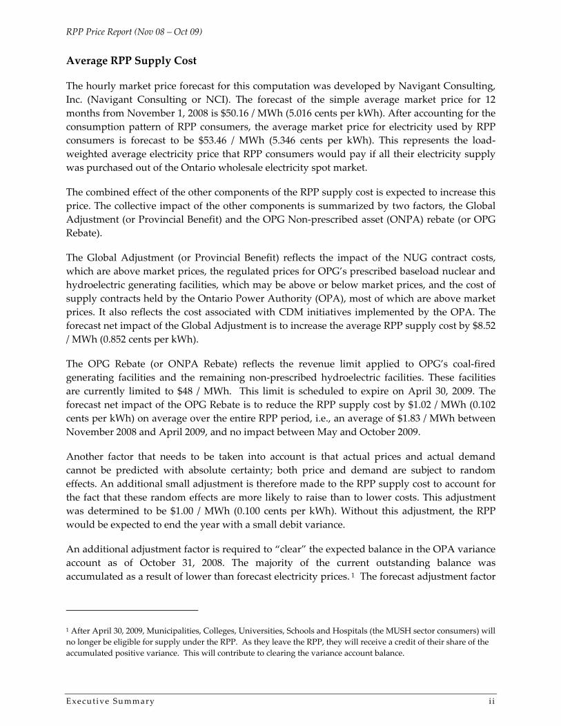
OEB Role in Determining Prices under the RPP
The OEB has a different role in calculating the commodity electricity prices that RPP consumers will pay relative to its role in regulating the distribution and transmission rates that utilities collect for delivering electricity to homes and businesses.
Distribution utilities file applications with the Board for approval of cost‐based charges levied on consumers for providing distribution services. The OEB scrutinizes these applications and sets reasonable rates to recover justifiable and prudent costs from consumers.
In contrast, for the RPP, the OEB forecasts the total cost of supplying the electricity used by RPP consumers and converts that cost into stable and predictable prices for RPP consumers. The forecast cost of supplying RPP consumers is based on a set of prices, most of which, unlike distribution rates, are not determined by the OEB. Some of these prices will be determined in the open market and will fluctuate hourly based on supply and demand. Some of these prices are determined by Government regulation or are based on contracts entered into by the OPA or the former Ontario Hydro. As of April 1, 2008, some are regulated by the OEB; that is, the payment amounts for OPG prescribed generators. Simply stated, the OEB does not currently regulate most of the electricity commodity prices or conservation costs which form the basis of the RPP Supply Cost in this RPP Price Report. In other words, while the OEB determines the electricity commodity prices that RPP consumers will pay, the OEB does not determine most of the various commodity prices and conservation costs that are blended together to set the RPP prices. In addition, unlike transmission and distribution rates, setting the RPP price does not involve an application or a rate order.

RPP Price Report (Nov 08 – Oct 09)
Table of Contents vi i
TABLE OF CONTENTS EXECUTIVE SUMMARY .............................................................................................................................................................I
AVERAGE RPP SUPPLY COST ....................................................................................................................................................... II CONVENTIONAL METER REGULATED PRICE PLAN..................................................................................................................... III SMART METER REGULATED PRICE PLAN .................................................................................................................................... IV
LIST OF FIGURES & TABLES ............................................................................................................................................. VIII 1. INTRODUCTION............................................................................................................................................................... 1
1.1 ASSOCIATED DOCUMENTS............................................................................................................................................. 1 1.2 PROCESS FOR RPP PRICE DETERMINATIONS ................................................................................................................. 2
2. CALCULATING THE RPP SUPPLY COST ................................................................................................................... 3 2.1 DEFINING THE RPP SUPPLY COST ................................................................................................................................. 3 2.2 COMPUTATION OF THE RPP SUPPLY COST.................................................................................................................... 4
2.2.1 Forecast Cost of Supply Under Market Rules .......................................................................................................... 5 2.2.2 Cost Adjustment Term for Prescribed Generators ................................................................................................... 8 2.2.3 Cost Adjustment Term for Non-Utility Generators (NUGs)................................................................................... 9 2.2.4 Cost Adjustment Term for Renewable Generation Under Output-Based Contracts with the OPA ........................ 9 2.2.5 Cost Adjustment Term for Other Contracts with the OPA ................................................................................... 10 2.2.6 Estimate of the Global Adjustment (or Provincial Benefit) .................................................................................... 12 2.2.7 Cost Adjustment Term for OPA Variance Account .............................................................................................. 12 2.2.8 Cost Adjustment Term for OPG Non-Prescribed Asset Rebate (or OPG Rebate) ................................................. 13
2.3 CORRECTING FOR THE BIAS TOWARDS UNFAVORABLE VARIANCES ........................................................................... 14 2.4 TOTAL RPP SUPPLY COST ........................................................................................................................................... 15
3. CALCULATING THE RPP PRICE................................................................................................................................. 18 3.1 SETTING THE TIER PRICES FOR RPP CONSUMERS WITH CONVENTIONAL METERS ..................................................... 18 3.2 SETTING THE TOU PRICES FOR CONSUMERS WITH ELIGIBLE TIME-OF-USE METERS .................................................. 18
4. EXPECTED VARIANCE .................................................................................................................................................. 21 APPENDIX A – MODELING VOLATILITY OF SUPPLY COST ...................................................................................... 23
INTRODUCTION .......................................................................................................................................................................... 23 THE MODEL OF SUPPLY COST VARIANCE .................................................................................................................................. 24 SIMULATING THE MODEL........................................................................................................................................................... 25 DERIVING PROBABILITY DISTRIBUTIONS .................................................................................................................................... 26 THE SUPPLY / DEMAND EFFECT ON MARKET PRICE ................................................................................................................. 27 COMPUTING RPP SUPPLY COST................................................................................................................................................. 27 VARIANCE RESULTS ................................................................................................................................................................... 27

RPP Price Report (Nov 08 – Oct 09)
Table of Contents vi i i
LIST OF FIGURES & TABLES
List of Figures
Figure 1: Process Flow for Determining the RPP Price ............................................................................................................. 2 Figure 2: Average Hourly RPP Consumption and Forecast HOEP for January.................................................................... 6 Figure 3: Average Hourly RPP Consumption and Forecast HOEP for July .......................................................................... 7 Figure 4: Ontario Generation by Category (% of kWh) .......................................................................................................... 15 Figure 5: Components of Total RPP Supply Cost (% of $)...................................................................................................... 16 Figure 6: Breakdown of Average RPP Consumption by TOU Periods................................................................................. 20 Figure 5: Expected Monthly Variance Account Balance ($ million)...................................................................................... 22 Figure 8: Diagram of Supply Cost Variance ............................................................................................................................. 24 Figure 9: Cumulative Variances over Entire Term .................................................................................................................. 28
List of Tables
Table 1: Ontario Electricity Market Price Forecast ($ per MWh) ............................................................................................. 5 Table 2: Average RPP Supply Cost Summary.......................................................................................................................... 17 Table 3: Price Paid by Average RPP Consumer under Tiered and TOU RPP prices .......................................................... 20

RPP Price Report (Nov 08 – Oct 09)
Introduct ion 1
1. INTRODUCTION Under amendments to the Ontario Energy Board Act, 1998 (the Act) contained in the Electricity Restructuring Act, 2004, the Ontario Energy Board (OEB or the Board) was mandated to develop a regulated price plan (RPP) for electricity prices to be charged to consumers that have been designated by regulation and have not opted to switch to a retailer. The first prices were implemented under the RPP effective on April 1, 2005, as set out in regulation by the Ontario Government. This report, and the prices contained herein are intended to be in effect on November 1, 2008 and remain in effect until October 31, 2009 barring any required true‐up or rebasing.4 The Board will review the prices in six months to determine if a change is needed.
The Board has prepared a Regulated Price Plan Manual (RPP Manual) to explain how the RPP price is set. It was prepared within the context of a larger regulatory proceeding (designated as RP‐2004‐0205) in which interested parties assisted the Board in developing the elements of the RPP.
This Report describes the way that the Board used the RPP Manual’s processes and methodologies to arrive at the RPP prices effective November 1, 2008.
This Report consists of four chapters and one appendix as follows:
o Chapter 1. Introduction
o Chapter 2. Calculating the RPP Supply Cost
o Chapter 3. Calculating RPP Prices
o Chapter 4. Expected Variance
o Appendix A. Modeling Volatility of Supply Cost
1.1 Associated Documents
Two documents are closely associated with this Report:
o The Regulated Price Plan Manual (RPP Manual) describes in detail the methodology followed in producing the results contained in this Report; and
o The Ontario Wholesale Electricity Market Price Forecast For the Period November 1, 2008 through April 30, 2010 (Market Price Forecast Report),5 prepared by Navigant Consulting Inc. (Navigant Consulting or NCI), contains the Ontario wholesale
4 In accordance with the RPP Manual, price resetting is considered for implementation every six months. If there is a price resetting following a Board review, it will determine how much of a price change will be needed to recover the forecast RPP supply cost plus or minus the accumulated variance in the OPA variance account over the next 12 months. In addition to the six month reconsideration, the RPP Manual allows for an automatic “trigger” based adjustment if the unexpected variance exceeds $160 million within a quarter.
5 The Market Price Forecast Report is posted on the OEB web site, along with the RPP Price Report, on the RPP web page.
RPP Price Report (Nov 08 – Oct 09)
Introduct ion 2
electricity market price forecast. The document details all of the assumptions which lie behind the hourly price forecast. Those assumptions are not repeated in this Report.
1.2 Process for RPP Price Determinations
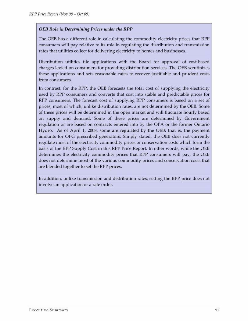
Figure 1 below illustrates the process for setting RPP prices. The RPP supply cost and the accumulated variance account balance (carried by the Ontario Power Authority or OPA) both contribute to the base RPP price, which is set to recover the full costs of electricity supply. The diagram below illustrates the processes to be followed to set the RPP price for both consumers with conventional meters and those with eligible time‐of‐use meters (or “smart” meters).
Figure 1: Process Flow for Determining the RPP Price
• Market Priced Generation• OPG Regulated Assets• NUGs• Contracted Renewables• Other Contracted Generation• Early Movers• OPG Non‐prescribed Asset
Rebate• OPA CDM Initiatives• Variance Clearance
• Market Priced Generation• OPG Regulated Assets• NUGs• Contracted Renewables• Other Contracted Generation• Early Movers• OPG Non‐prescribed Asset
Rebate• OPA CDM Initiatives• Variance Clearance Average RPP
PriceDetermination
Average RPP Price
Determination
RPP Supply Cost
RPP Supply Cost
Supply Cost
Volatility
Supply Cost
Volatility
Seasonal / TOU Price Analysis
Seasonal / TOU Price Analysis
TierAnalysisTier
AnalysisPrice for
Conventional Meters
Price for Conventional
Meters
Price for Eligible Time‐of‐Use
Meters
Price for Eligible Time‐of‐Use
Meters
• Market Priced Generation• OPG Regulated Assets• NUGs• Contracted Renewables• Other Contracted Generation• Early Movers• OPG Non‐prescribed Asset
Rebate• OPA CDM Initiatives• Variance Clearance
• Market Priced Generation• OPG Regulated Assets• NUGs• Contracted Renewables• Other Contracted Generation• Early Movers• OPG Non‐prescribed Asset
Rebate• OPA CDM Initiatives• Variance Clearance Average RPP
PriceDetermination
Average RPP Price
Determination
RPP Supply Cost
RPP Supply Cost
Supply Cost
Volatility
Supply Cost
Volatility
Seasonal / TOU Price Analysis
Seasonal / TOU Price Analysis
TierAnalysisTier
AnalysisPrice for
Conventional Meters
Price for Conventional
Meters
Price for Eligible Time‐of‐Use
Meters
Price for Eligible Time‐of‐Use
Meters
Source: RPP Manual
This Report is organized according to this basic process.

RPP Price Report (Nov 08 – Oct 09)
Calculat ing the RPP Supply Cost 3
2. CALCULATING THE RPP SUPPLY COST
The RPP supply cost calculation formula is set out in Equation 1 below. To calculate the RPP supply cost requires forecast data for each of the terms in Equation 1. Most of the terms depend on more than one underlying data source or assumption. This chapter details the data or assumption source for each of the terms and describes how the data were used to calculate the RPP supply cost. More detail on this methodology is in the RPP Manual.
It is important to remember that all of the terms in Equation 1 are forecasts. In some cases, the calculation uses actual historical values, but in these cases the historical values constitute the best available forecast.
2.1 Defining the RPP Supply Cost
Equation 1 below defines the RPP supply cost. The elements of Equation 1 are set out by the legislation and regulations. This equation is further explained in the RPP Manual.
Equation 1
CRPP = M + α [(A – B) + (C – D) + (E – F) + G] + H, where
o CRPP is the total RPP supply cost;
o M is the amount that the RPP supply would have cost under the Market Rules;
o α is the RPP proportion of the total demand in Ontario;6
o A is the amount paid to prescribed (or regulated) generators;7
o B is the amount those generators would have received under the Market Rules;
o C is the amount paid to non‐utility generators (NUGs) under existing contracts;
o D is the amount those NUGs would have received under the Market Rules for both electricity and ancillary services;
o E is the amount paid to generators contracted to the OPA that are paid according to their output (i.e., renewable generators);
o F the amount those generators would have received under the Market Rules;
6 The expression in square brackets is the Global Adjustment; it is applied to the RPP according to the load ratio share represented by RPP consumers, denoted here as α.
7 These are generators designated by regulation and whose output is subject (in whole or in part) to regulated payment amounts that were set by Government regulation. These regulated payment amounts are now set by the Board. A Board proceeding (EB‐2007‐0905) was recently completed. The Board denied a request for interim payment amounts and a final Board decision is expected in the near future.

RPP Price Report (Nov 08 – Oct 09)
Calculat ing the RPP Supply Cost 4
o G is the amount paid by the OPA for its other procurement contracts, which includes payments to conventional generators (i.e., natural gas,), and for demand response or conservation and demand management (CDM); and
o H is the amount associated with the variance account held by the OPA. This includes any existing variance account balance needed to be recovered (or disbursed) in addition to any interest incurred (or earned).
The forecast per unit RPP supply cost will be the total RPP supply cost (CRPP) divided by the total forecast RPP demand. RPP prices will be based on that forecast per unit cost.
The OPG Non‐prescribed Asset (ONPA) Rebate (or OPG Rebate) is not included in Equation 1 because it did not exist at the time the RPP Manual was developed and it has always been intended to be temporary in nature. The OPG Rebate is however addressed in Section 2.2.8 of this report and is considered as an after‐the‐fact adjustment to the total RPP Supply Cost.
2.2 Computation of the RPP Supply Cost
Broadly speaking, the steps involved in forecasting the RPP supply cost are:
1. Forecast wholesale market prices;
2. Forecast the load shape for RPP consumers;
3. Forecast the quantities in Equation 1; and
4. Forecast RPP Supply Cost = Total of Equation 1.
In addition to the four steps listed above, the calculation of the total RPP supply cost requires a forecast of the OPG Rebate and a forecast of the stochastic adjustment, which are not included in Equation 1. As mentioned previously, the OPG Rebate is not included in Equation 1 because it did not exist at the time the RPP Manual was developed. The stochastic adjustment is included in the RPP Manual as an additional cost factor calculated outside of Equation 1. Since the RPP prices are always announced by the Board in advance of the actual price adjustment being implemented, it is also necessary to forecast the net variance account balance at the end of the current RPP period (October 31, 2008).8
The discussion of data and computation for the forecast of the RPP supply cost will describe each term or group of terms in Equation 1, the data used for forecasting them, and the computational methodology to produce each component of the RPP supply cost.
8 RPP prices are announced in advance by the Board to provide notification to consumers of the upcoming price change and to provide distributors with the necessary amount of time to incorporate the new RPP prices into their billing systems.

RPP Price Report (Nov 08 – Oct 09)
Calculat ing the RPP Supply Cost 5
2.2.1 Forecast Cost of Supply Under Market Rules
This section covers the first term of Equation 1:
CRPP = M + α [(A – B) + (C – D) + (E – F) + G] +H.
The forecast cost of supply to RPP consumers under the Market Rules depends on two forecasts:
o The forecast of the hourly Ontario electricity price (HOEP) in the IESO‐administered market in each hour of the year; and
o The forecast of demand from RPP consumers in each hour of the year.
The forecast of HOEP is taken directly from the Ontario Market Price Forecast Report. The Ontario Market Price Forecast Report also contains a detailed explanation of the assumptions that underpin the forecast such as generator fuel prices (e.g., coal and natural gas). Table 1 below shows forecast seasonal on‐peak, off‐peak, and average prices. The prices provided in Table 1 are simple averages over all of the hours in the specified period (i.e., they are not load‐weighted). These on‐peak and off‐peak periods differ from and should not be confused with the TOU periods associated with the RPP TOU prices discussed later in this report.
Table 1: Ontario Electricity Market Price Forecast ($ per MWh)
Term Quarter Calendar Period On-Peak Off-Peak Average Term Average
RPP
Yea
r Q1 Nov 08 - Jan 09 $60.70 $40.04 $49.47Q2 Feb 09 - Apr 09 $60.80 $41.79 $50.49Q3 May 09 - Jul 09 $62.17 $34.32 $47.17Q4 Aug 09 - Oct 09 $68.50 $41.14 $53.54 $50.16R
PP Y
ear
Oth
e r Q1 Nov 09 - Jan 10 $65.12 $42.12 $52.63Q2 Feb 10 - Apr 10 $59.37 $39.58 $48.62 $50.66O
ther
Source: Navigant Consulting, Wholesale Electricity Market Price Forecast Report
Note: On‐peak hours include the hours ending at 8 a.m. through 11 p.m. Eastern Standard Time (EST) on working weekdays and off‐peak hours include all other hours.
The forecast of the hourly electricity demand from RPP consumers comes from forecasts of the fraction of their total load consumed in each hour (their load shape) and the fraction that they represent of the total system‐wide load for all consumers in Ontario. The forecast load shape of RPP consumers was based on historic hourly RPP consumer load data for virtually all Ontario electricity distributors from the Board’s Cost Allocation Review process (EB‐2005‐0317). Load shapes change very slowly, so this is a reasonable approximation.9
9 Prior to obtaining this more accurate hourly load data, previous RPP prices were established based on an approximation widely used called the Net System Load Shape, or NSLS. The hourly load data from the Board’s Cost Allocation process will result in more accurate time‐of‐use prices.

RPP Price Report (Nov 08 – Oct 09)
Calculat ing the RPP Supply Cost 6
Figure 2 presents a chart of the forecast average hourly RPP loadshape and HOEP for January. This chart clearly demonstrates that RPP consumption is higher during those times of the day when prices are forecast to be higher. HOEP is based on, among other things, total system demand; hence there are factors outside RPP consumption that impact the price in each hour of the day.
Figure 2: Average Hourly RPP Consumption and Forecast HOEP for January
0
2,000
4,000
6,000
8,000
10,000
12,000
0:00 3:00 6:00 9:00 12:00 15:00 18:00 21:00 0:00
RPP
Dem
and
(MW
)
$0
$20
$40
$60
$80
HO
EP ($
/MW
h)
DemandHOEP
Source: NCI Note: All times are EST

RPP Price Report (Nov 08 – Oct 09)
Calculat ing the RPP Supply Cost 7
Figure 3 presents the same information for July. Again, this chart clearly demonstrates that RPP consumption is higher during times when prices are forecast to be higher.
Figure 3: Average Hourly RPP Consumption and Forecast HOEP for July
0
2,000
4,000
6,000
8,000
10,000
12,000
0:00 3:00 6:00 9:00 12:00 15:00 18:00 21:00 0:00
RPP
Dem
and
(MW
)
$0
$20
$40
$60
$80
HO
EP ($
/MW
h)
DemandHOEP
Source: NCI Note: All times are EST
A similar pattern is observed in monthly RPP consumption. RPP consumption is higher during those months when prices are forecast to be higher.
The forecast of the market‐based component of the RPP supply cost is therefore the demand of RPP consumers times the HOEP at the time of consumption. As shown in Table 1 on page 5, the forecast simple average HOEP for the period November 1, 2008 to October 31, 2009, is $50.16 / MWh (5.016 cents per kWh). Based on the forecast RPP consumption pattern, the load weighted average price for RPP consumers is $53.46 / MWh (5.346 cents per kWh).
The amount of electricity supplied under the RPP depends on which consumers are eligible to receive the RPP. Currently, consumers eligible for the RPP include residential consumers, small commercial consumers, farms, and “designated” consumers including municipalities, universities, colleges, schools, hospitals, as well as any other consumers whose annual usage is 250,000 kWh or less. The Ontario government amended Regulation 95/05 in March 2008 to maintain the current RPP eligibility criteria until May 1, 2009. At that time, municipalities, universities, colleges, schools, and hospitals will no longer be eligible for the RPP. Residential consumers, small businesses, farms and any other consumers whose annual usage is 250,000 kWh or less will continue to be eligible.

RPP Price Report (Nov 08 – Oct 09)
Calculat ing the RPP Supply Cost 8
RPP Attrition
Since the RPP was introduced, some consumers have chosen to leave the RPP program to sign competitive retail supply contracts. Some RPP consumers with interval meters have also chosen to purchase power in the spot market instead of under the RPP. Some consumers have also returned to the RPP from retail contracts. The expected impact of this migration away from the RPP (or attrition) has been reflected in the forecast volume of RPP consumers for the period under consideration, but is not expected to have a pronounced impact on the load shape of RPP consumers for the period under consideration.
For this Report, the calculations of the RPP Supply Cost has taken into account the impact on RPP consumption of the consumers who will be required to exit the RPP on or before May 1, 2009 (that is, for half of the period covered by this Report.)
With respect to the total volume of RPP consumers, all of the factors contributing to the average RPP supply cost are expressed in $ / MWh (or cents per kWh). Hence, if the volume were significantly different from the forecast but all other factors (such as load shape, fuel prices, and generator availability) remain unchanged, the average RPP supply cost would not change.
RPP migration to competitive retail supply or the spot market price is a potential risk factor in determining the RPP supply cost and will continue to be tracked closely.
The current eligibility criteria result in RPP consumers accounting for 43.5% of the total electricity withdrawn in the province over the past year (September 2007 through August 2008). Based on the rate of attrition to date, and the departure of the large MUSH sector consumers that have remained on the RPP, it is forecast that RPP consumption will represent about 57 TWh or 39.2% of the total electricity withdrawn in Ontario over the forecast period.
The value of α is therefore 0.392.
2.2.2 Cost Adjustment Term for Prescribed Generators
This section covers the second term of Equation 1:
CRPP = M + α [(A – B) + (C – D) + (E – F) + G] + H
The prescribed generators are comprised of the nuclear and baseload hydroelectric facilities of Ontario Power Generation (OPG). The forecast of the dollar amount that the prescribed generators would receive under the Market Rules (quantity B in Equation 1) was calculated as their forecast monthly generation multiplied by their forecast average market revenue in each month. Forecasts of both of these variables were taken from Navigant Consulting’s statistical model. For details of the statistical model and the wholesale market price forecast, see the Navigant Consulting Wholesale Market Price Forecast Report.

RPP Price Report (Nov 08 – Oct 09)
Calculat ing the RPP Supply Cost 9
The amount paid to the prescribed generators (quantity A in Equation 1) is currently determined by the Ontario Energy Board. Government regulation had set the payment amounts for the prescribed hydroelectric assets at $33 / MWh for up to 1,900 MW in any hour, while the payment amounts for the prescribed nuclear assets was set at $49.50 / MWh. OPG has applied to the Board for an increase in these payment amounts. The current payments were determined to be interim effective April 1, 2008. The hearing of OPG’s application has concluded but the Board has not yet issued a decision and order.
The Board believes that it would be prudent to take into account some effect of OPG’s application for increased payment amounts. This approach is consistent with one of the objectives of the RPP which is to smooth changes in prices over time. Therefore, 50% of the increase requested by OPG in its application has been used for the purpose of calculating the RPP prices. For forecasting purposes, the payment amounts are therefore $35.50 / MWh for hydroelectric output and $53 / MWh for nuclear output, with an assumed implementation date of December 1, 2008 and no assumptions on retroactive recovery.
Regardless of whether the Board ultimately approves higher or lower payments, the difference will be captured in the variance account dedicated to the RPP. That difference will be reflected in RPP prices when they are reset for May 1, 2009. At that time, the final payment amounts approved by the Board will also be incorporated in RPP prices.
Quantity A was therefore forecast by multiplying these fixed payment amounts per MWh for the prescribed generators times their total forecast output per month in MWh.
2.2.3 Cost Adjustment Term for Non‐Utility Generators (NUGs)
This section describes the calculation of the third term of Equation 1:
CRPP = M + α [(A – B) + (C – D) + (E – F) + G] + H
The amount that the NUGs would receive under the Market Rules, quantity D in Equation 1, is their hourly production times the hourly Ontario energy price. These quantities were forecast on a monthly basis, as an aggregate for the NUGs as a whole, in Navigant Consulting’s statistical model.
The Ontario Power Authority recently published monthly aggregate payments to the NUGs between September 2007 and August 2008. Although the details of these payments (amounts by recipient, volumes, etc.) are not public, the published information has been used as the basis for forecasting payments in future months. This forecast was used to compute an estimate of the total payments to the NUGs under their contracts, or amount C in Equation 1.
2.2.4 Cost Adjustment Term for Renewable Generation Under Output‐Based Contracts with the OPA
This section describes the calculation of the fourth term of Equation 1:
RPP Price Report (Nov 08 – Oct 09)
Calculat ing the RPP Supply Cost 10
CRPP = M + α [(A – B) + (C – D) + (E – F) + G] + H
Quantities E and F in the above formula refer to generators paid by the OPA under contracts related to output. Generators in this category are renewable generators contracted under the Renewable Energy Supply (RES) Request for Proposals (RFP) Phase I and II and the Renewable Energy Standard Offer Program (RESOP).
The size and generation type of the successful renewable energy projects have been announced by the Ministry of Energy (MoE) and the OPA. The statistical model produced forecasts of their monthly output, using either historical values of actual outputs (where available), or estimates based on the plants’ capacities and estimated capacity factors. The statistical model also forecast average market revenues for each plant or type of plant. Quantity F in Equation 1 is therefore the forecast output of the renewable generation multiplied by the forecast average market revenue at the time that output is generated.
Quantity E in Equation 1 is the forecast quantity of electricity supplied by these renewable generators times the fixed price they are paid under their contract with the OPA. The MoE released the weighted average price for both Renewable RFP I and Renewable RFP II; they are $79.97 / MWh and $86.40 / MWh respectively. Under RESOP, photovoltaic (solar) generation is paid 42¢ / kWh, and all other types of renewable generation are paid 11¢ / kWh plus, in some cases, 3.52¢ / kWh for production during on‐peak hours. This extra payment of 3.52¢ / kWh is generally limited to those generators that are able to reliably provide on‐peak generation.10
2.2.5 Cost Adjustment Term for Other Contracts with the OPA
This section describes the calculation of the fifth term of Equation 1:
CRPP = M + α [(A – B) + (C – D) + (E – F) + G] + H
The costs for three types of resources under contract with the OPA are included in G:
1. conventional generation (e.g., natural gas) whose payment relates to the generator’s capacity costs;
2. demand side management or demand response contracts; and
3. Bruce Power whose generation from its Bruce A nuclear facility is under an output‐based contract.
The contribution of conventional generation under contract to the OPA to quantity G relates to several contracts:
10 The OPA has contracted with various small renewable energy power producers under the RESOP. If the projects come into service as planned under their contracts, this program would add the following amount of capacity during the forecast period: 524 MW of wind, 54 MW of hydroelectric and biomass, and 264 MW of photovoltaic (solar).

RPP Price Report (Nov 08 – Oct 09)
Calculat ing the RPP Supply Cost 11
o The Clean Energy Supply (CES) RFP, which includes conventional generation contracts as well as a 10‐MW demand response contract awarded to Loblaws11
o The “early mover” contracts12
o Seven contracts awarded through the Combined Heat and Power (CHP) Phase I RFP13
o Four large gas‐fired plants (Portlands, Goreway, Greenfield and St. Clair). The first of these, the Portlands Energy Centre, began operation as a simple‐cycle plant in June 2008 and is currently being converted into a combined‐cycle plant. The other three plants are expected to come into service in the last quarter of 2008 or the first quarter of 2009.
The costs of these contracts are based on an estimate of the contingent support payments to be paid out under the contract guidelines. The contingent support payment is the difference between the net revenue requirement (NRR) stipulated in the contracts and the “deemed” energy market revenues. The deemed energy market revenues were estimated based on the deemed dispatch logic as stipulated in the contract and the wholesale market price forecast that underpins this RPP price setting activity. The NRRs and other contract parameters for each contract have been estimated based on publicly available information. For example, the average NRR for the CES contracts was announced by the Ministry of Energy to be $7,900 per megawatt‐month.14
The cost to the OPA of any additional conservation and demand management (CDM) initiatives is also captured in term G of Equation 1. The OPA is currently offering or planning to offer several CDM initiatives over the next 12 months. These programs generally fall into three categories: Mass Market programs, Commercial / Institutional Market programs, and Industrial Market programs. Some OPA conservation‐related costs are not recovered through the Global Adjustment and therefore do not impact the Global Adjustment (i.e., are not included in term G of Equation 1). Such costs will instead be recovered through the OPA Fee as part of the Regulatory charge.
The Bruce Power contract initially stipulated that output from the Bruce A facility would be paid a base price of $57.37 / MWh, indexed to inflation, plus fuel costs. As of April 1, 2008, the
11 Six facilities holding CES contracts are expected to be operational during this RPP period: the GTAA Cogeneration Facility, the Loblaws Demand Response Program, the Greenfield Energy Centre, the Portlands Energy Centre, the Goreway Station Project, and the St. Clair Energy Centre.
12 Five facilities signed early mover contracts with the OPA: the Brighton Beach facility, TransAlta’s Sarnia facility, and three Toromont facilities. These contracts will remain in force until 2011.
13 Six facilities holding CHP Phase I contracts are expected to be operational during this RPP period: the Great Northern Tri‐gen Facility, the Durham College District Energy Project, the Countryside London Cogeneration Facility, the Warden Energy Centre, the Algoma Energy Cogeneration Facility, and the East Windsor Cogeneration Centre.
14 Given the ministerial directive to the OPA, the NRR for the “early movers” was assumed to be the same.

RPP Price Report (Nov 08 – Oct 09)
Calculat ing the RPP Supply Cost 12
base price was increased by $2.11 / MWh, to $59.48 / MWh.15 At today’s fuel prices and including inflation adjustments since the contract went into effect, the average price during the upcoming RPP period is estimated to be approximately $69 / MWh. Under the agreement, Bruce Power will be paid a monthly contingent support payment if its actual revenues are less than contract revenues or it will make a revenue sharing payment to the Province if actual revenues are greater than contract revenues. The Bruce Power contract also stipulates that output from the Bruce B facility be guaranteed a floor price of $45 / MWh, indexed to inflation, over a calendar year. Adjustments for inflation are made on an annual basis. For the upcoming RPP period, the average floor price is forecast to be approximately $48 / MWh. Payments are calculated on both a monthly and an annual basis, with the result that any payments made are usually repaid in the following year.
2.2.6 Estimate of the Global Adjustment (or Provincial Benefit)
The overall impact of the central term in Equation 1 – α [(A – B) + (C – D) + (E – F) + G] – is forecast to increase the RPP unit cost by $8.52 / MWh (0.852 cents per kWh). This essentially represents the forecast of the average Global Adjustment that would accrue to RPP consumers over the period from November 1, 2008 to October 31, 2009.
The contract awarded to OPG’s Lennox generation facility regarding reliability must‐run (RMR) status is not between OPG and the OPA, but between OPG and the Independent Electricity System Operator (IESO). Hence, the cost of the contract is not recovered through the global adjustment and is not included in the RPP supply cost. The cost will instead be recovered through the hourly uplift charge.16
2.2.7 Cost Adjustment Term for OPA Variance Account
This section describes the calculation of the sixth term of Equation 1:
CRPP = M + α [(A – B) + (C – D) + (E – F) + G] + H
The cost adjustment term for the OPA variance account consists of two factors. The first is the forecast interest costs associated with carrying any RPP‐related variances incurred during the upcoming RPP period (November 2008 – October 2009). The second represents the price adjustment required to clear (i.e., recover or disburse) the existing RPP variance and interest accumulated over the previous RPP period.
15 The “base” (or “reference”) price was increased due to the agreement involving the expansion of the Bruce A refurbishment project.
16 The hourly uplift charge includes wholesale electricity market services which, in part, are provided by the IESO to ensure reliability of the system. RPP consumers do not see this charge on the simplified bill. For RPP consumers, this means that the costs associated with OPG’s Lennox facility will ultimately be recovered through the Regulatory charge on consumer bills. This charge includes the hourly uplift charge.

RPP Price Report (Nov 08 – Oct 09)
Calculat ing the RPP Supply Cost 13
The first term discussed above is small, as any interest expenses incurred by the OPA to carry consumer debit variances in some months are generally offset by interest income the OPA receives from carrying consumer credit balances in other months. In addition, the interest rate paid by the OPA on the variance account is relatively low.
The second term is significant, as it represents the price adjustment necessary to clear the total net variance accumulated since the RPP was introduced on April 1, 2005 through to October 31, 2008. As of October 31, 2008 the net variance account balance is expected to be a favourable or positive balance of approximately $101 million including interest. This has declined since May 1, 2008 as consumers have received a credit in RPP prices to draw down the positive variance.
For this Report, an additional factor needs to be considered in forecasting the variance account balance. That is, the payments to be made to the MUSH sector consumers, through the Final RPP Variance Settlement Amount, as they leave the RPP. Based on the assumption that MUSH sector consumption, as a proportion of total RPP consumption, has already declined by approximately 50%, the remaining MUSH sector consumers are expected to receive a total of approximately $8 million when they leave the RPP supply on April 30, 2009. While that amount will no longer be available as a credit to the remaining RPP consumers, it does not significantly affect their credit per kWh, because the MUSH consumer exit removes a proportionate amount of the RPP demand.
A variance clearance factor has been calculated that is estimated to bring the variance account to approximately a zero balance over the twelve month period, after taking into account both the changes in total RPP consumption and the Final RPP Variance Settlement Amount payments expected as of October 31, 2008. This variance clearance factor has been decreased from a credit of 0.352 cents per kWh in the previous RPP report to a credit of 0.166 cents per kWh. This decrease is due to a lower forecast variance account balance as the net variance balance has been reduced by the credits paid to RPP consumers. The impact of this term is to decrease the average RPP supply cost by the amount of the credit: $1.66 / MWh (0.166 cents per kWh).
2.2.8 Cost Adjustment Term for OPG Non‐Prescribed Asset Rebate (or OPG Rebate)
On February 23, 2005 the Ontario Government announced a partial revenue limit on the non‐prescribed assets (i.e., non‐baseload hydroelectric and coal generation facilities) owned by OPG. The regulation limited a portion of the revenues from OPG’s non‐prescribed facilities to $47 / MWh for a 13 month period ending April 30, 2006. An estimate of the rebate paid to consumers resulting from this revenue limit was included in the initial RPP price implemented on April 1, 2005. The rebate is called either the OPG Non‐Prescribed Asset (ONPA) Rebate, or the OPG Rebate.
On February 9, 2006, the Ontario Government announced that the partial revenue limit had been extended through April 2009. However, some of the terms were also revised.
o The revenue limit is currently $48 / MWh.

RPP Price Report (Nov 08 – Oct 09)
Calculat ing the RPP Supply Cost 14
o In addition, the rebate is paid out on a quarterly basis as opposed to at the end of the term.
The OPG Rebate is also affected by the volumes sold through the OPA administered forward contract Pilot Auction (PA) program. Volumes sold by OPG through the PA, which are from the ONPA assets, are subject to a revenue limit of $51 / MWh as opposed to $48 / MWh. The rebate contribution from the volumes sold through the PA is calculated as the difference between the auction selling price and the cap price of $51 / MWh.
After April 30, 2009, these OPG assets will no longer be subject to a revenue limit. In the RPP calculation, they are assumed to earn HOEP beginning May 1, 2009.
The OPG Rebate is forecast to be $1.83 / MWh on average during the first half of the forecast period (November 2008 to April 2009). In the second half of the period, there is expected to be no rebate. With this rebate included in the calculation of the RPP supply cost, as required by Government regulation, there is a $1.02 / MWh (0.102 cents per kWh) forecast reduction in the average RPP supply cost over the entire forecast period.17 This term is not included in Equation 1, but is considered part of the total RPP supply cost.
2.3 Correcting for the Bias Towards Unfavorable Variances
All of the supply costs discussed in section 2.2 are based on a forecast of the HOEP. However, actual prices and actual demand cannot be predicted with absolute certainty. Calculating the total RPP supply cost therefore needs to take into account the fact that volatility exists amongst the forecast parameters, and that there is a slightly greater likelihood of negative or unfavourable variances than favourable variances. For example, since nuclear generation plants tend to operate at capacity factors between 80% and 90%, these facilities are more likely to “under‐generate” (due to unscheduled outages) than to “over‐generate” (i.e., there is 10‐20% upside versus 80‐90% downside on the generator output). Similarly, during unexpectedly cold or hot weather, prices tend to be higher than expected as does RPP consumers’ demand for electricity. The net result is that the RPP would be ʺexpectedʺ to end the year with a small unfavourable variance in the absence of a minor adjustment to reflect the greater likelihood of unfavourable variances. This adjustment term is referred to as the “stochastic adjustment”. The term stochastic is a reference to the use of probabilistic modeling techniques in determining this adjustment.
These unfavourable variances not only have an effect on the market priced component of the RPP supply cost, but also on the Global Adjustment and OPG Rebate components as well. For example, in the scenario of nuclear generation used in the previous paragraph, an unforeseen decline in OPG’s nuclear production will not only have an impact on the market price as more expensive generation alternatives are required to fill the void, but terms A and B from Equation
17 Included in this term is an estimate of the interest cost to be incurred by the OPA as a result of the lag associated with the quarterly payment structure.

RPP Price Report (Nov 08 – Oct 09)
Calculat ing the RPP Supply Cost 15
1 are also affected. Likewise an unforeseen decline in Bruce Power’s nuclear production would have a similar impact on market prices, in addition to an impact on term G in Equation 1. For a detailed discussion of methodology used to model the unfavourable variances please see Appendix A of this report.
Inclusive of all the factors discussed above, and in Appendix A, the necessary stochastic adjustment was determined to be $1.00 / MWh (0.100 cents per kWh). This amount is included in the price paid by RPP consumers to ensure that the “expected” variance at the end of the RPP year is zero.
2.4 Total RPP Supply Cost
With these additional factors (OPG Rebate and stochastic adjustment) taken into consideration, the total RPP supply cost is estimated to be approximately $3.65 billion.18 Figure 4 breaks this supply cost into the four major cost streams. “Market‐based generation” includes a small amount of output from OPG’s non‐prescribed assets that is not subject to either the regulated price or the revenue limit based on the provisions of the regulations governing these mechanisms.
Figures 4 and 5 below illustrate different concepts. Figure 4 shows the expected breakdown of physical electricity (i.e., kilowatt‐hours) supplied by each of the four generation categories during the upcoming RPP period. This includes all Ontario generation, not just that used by RPP consumers.
Figure 4: Ontario Generation by Category (% of kWh) OPG Non-Prescribed
20%
Other Contracts
20%
Market-Based18%
OPG Prescribed
42%
Source: NCI
18 The total cost figure is net of the forecast variance account balance as of October 31, 2008.
RPP Price Report (Nov 08 – Oct 09)
Calculat ing the RPP Supply Cost 16
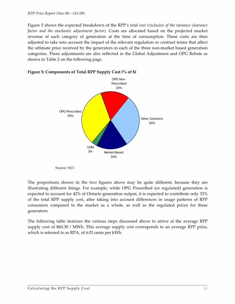
Figure 5 shows the expected breakdown of the RPP’s total cost (exclusive of the variance clearance factor and the stochastic adjustment factor). Costs are allocated based on the projected market revenue of each category of generation at the time of consumption. These costs are then adjusted to take into account the impact of the relevant regulation or contract terms that affect the ultimate price received by the generators in each of the three non‐market based generation categories. These adjustments are also reflected in the Global Adjustment and OPG Rebate as shown in Table 2 on the following page.
Figure 5: Components of Total RPP Supply Cost (% of $) OPG Non-Prescribed
16%
Other Contracts30%
Market-Based18%
CDM3%
OPG Prescribed33%
Source: NCI
The proportions shown in the two figures above may be quite different, because they are illustrating different things. For example, while OPG Prescribed (or regulated) generation is expected to account for 42% of Ontario generation output, it is expected to contribute only 33% of the total RPP supply cost, after taking into account differences in usage patterns of RPP consumers compared to the market as a whole, as well as the regulated prices for these generators.
The following table itemizes the various steps discussed above to arrive at the average RPP supply cost of $60.30 / MWh. This average supply cost corresponds to an average RPP price, which is referred to as RPA, of 6.03 cents per kWh.

RPP Price Report (Nov 08 – Oct 09)
Calculat ing the RPP Supply Cost 17
Table 2: Average RPP Supply Cost Summary
RPP Supply Cost Summary
for the period from November 1, 2008 through October 31, 2009Forecast Wholesale Electricity Price $50.16
Load‐Weighted Price for RPP Consumers ($ / MWh) $53.46Impact of the Global Adjusment ($ / MWh) + $8.52Impact of the OPG Non‐prescribed Asset Rebate ($ / MWh) + ($1.02)Adjustment to Address Bias Towards Unfavourable Variance ($ / MWh) + $1.00Adjustment to Clear Existing Variance ($ / MWh) + ($1.66)
Average Supply Cost for RPP Consumers ($ / MWh) = $60.30 Source: NCI

RPP Price Report (Nov 08 – Oct 09)
Calculat ing the RPP Price 18
3. CALCULATING THE RPP PRICE
The previous chapter calculated a forecast of the total RPP supply cost. Given the forecast of total RPP demand, it also produced a computation of the average RPP supply cost and the average RPP supply price, RPA. This chapter will detail the determination of the prices for the tiers, RPCMT1 and RPCMT2, and the determination of the prices for consumers with eligible time‐of‐use (TOU) meters that are being charged the TOU prices, RPEMON, RPEMMID, and RPEMOFF.
3.1 Setting the Tier Prices for RPP Consumers with Conventional Meters
The final step in setting the price for RPP consumers with conventional meters is to determine the tier prices for RPP consumers with conventional meters. For such consumers, there is a tiered pricing structure with two price tiers — RPCMT1 (the price for consumption at or below the tier threshold) and RPCMT2 (the price for consumption above the tier threshold). The tier threshold is an amount of consumption per month.
The tier prices are calculated such that the average revenue generated is equal to the RPA. This is achieved by maintaining the ratio between the original upper and lower tier prices (in other words, the ratio between 4.7 and 5.5 cents per kWh) and forecasting consumption above and below the threshold in each month of the RPP.
The resulting tier prices are:
o RPCMT1 = 5.6 cents per kWh, and
o RPCMT2 = 6.5 cents per kWh.
3.2 Setting the TOU Prices for Consumers with Eligible Time‐of‐Use Meters
The average RPP price for consumers with eligible time‐of‐use meters is the same as that for conventional meters, the RPA.19 For those consumers whose distributors have chosen to make time‐of‐use (TOU) prices available, three separate prices will apply. The times when these prices will apply will vary by time of day and season, as set out in the RPP Manual. There are three price levels: On‐peak (RPEMON), Mid‐peak (RPEMMID), and Off‐peak (RPEMOFF). The load‐weighted average price must be equal to the RPA, as was the case for the conventional meter RPP prices.
As described in the RPP Manual, the first step is to set the Off‐peak price, or RPEMOFF. This price reflects the forecast market price during that period, adjusted by the global adjustment,
19 In future years, when experience with time‐of‐use meters produces a more accurate load shape for consumers with eligible time‐of‐use meters, the average prices could differ, depending on how different the actual load shape of the time‐of‐use meter consumers is from the other RPP consumers.

RPP Price Report (Nov 08 – Oct 09)
Calculat ing the RPP Price 19
the variance clearance factor and the OPG Rebate. The Mid‐peak price, RPEMMID, was similarly set. Once these two prices are set, and given the forecast levels of consumption during each of the three periods, the On‐peak price, RPEMON, is determined by the need to make the load‐weighted average price equal to the RPA. Approximately one quarter of the stochastic adjustment was allocated to the Mid‐peak price and three quarters was allocated to the On‐peak price as this is when the majority of the risks being covered by the adjustment tend to be borne.
The resulting time‐of‐use prices are:
o RPEMOFF = 4.0 cents per kWh
o RPEMMID = 7.2 cents per kWh, and
o RPEMON = 8.8 cents per kWh.
As defined in the RPP Manual, the time periods for time‐of‐use (TOU) price application are defined as follows:
o Off‐peak period (priced at RPEMOFF):
Winter and summer weekdays: 10 p.m. to midnight and midnight to 7 a.m.
Winter and summer weekends and holidays:20 24 hours (all day)
o Mid‐peak period (priced at RPEMMID)
Winter weekdays (November 1 to April 30): 11 a.m. to 5 p.m. and 8 p.m. to 10 p.m.
Summer weekdays (May 1 to October 31): 7 a.m. to 11 a.m. and 5 p.m. to 10 p.m.
o On‐peak period (priced at RPEMON)
Winter weekdays: 7 a.m. to 11 a.m. and 5 p.m. to 8 p.m.
Summer weekdays: 11 a.m. to 5 p.m.
The above times are given in local time (i.e., the times given reflect daylight savings time in the summer).
The average price a consumer on time‐of‐use prices will pay will depend on the consumer’s load profile (i.e., how much electricity is used at what time). As discussed above, RPP prices are set so that a consumer with an average load profile will pay the same average price under either prices, as shown in Table 3. This average price is equal to the average RPP supply cost (the RPA) of 6.03¢ / kWh.
20 For the purpose of RPP time‐of‐use pricing, a “holiday” includes the following days: New Year’s Day, Family Day, Good Friday, Christmas Day, Boxing Day, Victoria Day, Canada Day, Labour Day, Thanksgiving Day, and the Civic Holiday. When any holiday falls on a weekend (Saturday or Sunday), the next weekday following is to be used in lieu of that holiday.

RPP Price Report (Nov 08 – Oct 09)
Calculat ing the RPP Price 20
Table 3: Price Paid by Average RPP Consumer under Tiered and TOU RPP prices
Tiered RPP Prices Tier 1 Tier 2 Average Price
Rate 5.6¢ 6.5¢ 6.0¢
% of Consumption 55% 45%
Time‐of‐Use RPP Prices Off‐Peak Mid‐Peak On‐Peak Average Price
Price 4.0¢ 7.2¢ 8.8¢ 6.0¢
% of Consumption 50% 24% 26%
As shown in Figure 6, 50% of the consumption of consumers with the same consumption pattern as the average RPP consumer currently paying TOU prices will be at the Off‐Peak price. The breakdown of consumption of the average RPP consumer in each of the three TOU periods is shown in Figure 6.21
Figure 6: Breakdown of Average RPP Consumption by TOU Periods
On-Peak, 26%
Mid-Peak, 24%
Off-Peak, 50%
Based on experience in other jurisdictions where TOU pricing has been implemented, some degree of shifting from the higher priced periods to the lower priced periods occurs, so the percentage of consumption in the On‐Peak period would be expected to decrease over time. However, given the limited experience in Ontario with TOU pricing to date, the breakdown shown in Figure 6 above does not currently take into account the potential impact of such shifting.
21 The Off‐Peak TOU price applies for more than 55% of the hours in a typical week. The On‐Peak period TOU price applies for 18% of the hours in a summer week and, because the On‐Peak period changes in the winter, applies for just over 20% of the hours in a winter week. The Mid‐Peak price applies during the remaining hours; that is, 27% of the hours in a summer week and 24% of the hours in a winter week.

RPP Price Report (Nov 08 – Oct 09)
Expected Variance 21
4. EXPECTED VARIANCE
Once the RPP prices are set, the monthly expected variance can be calculated directly. The variance clearance factor is set so that the expected variance balance at the end of the RPP period will be zero. However, the variance balance is not expected to decline smoothly; the amount of the variance balance cleared is expected to vary significantly from month to month for several reasons:
• Variance clearance will tend to be higher in months when RPP volumes are higher (i.e., summer and winter) and lower when volumes are lower (i.e., spring and fall).
• While there is only technically a single average RPP price (or RPA) in this report, the RPP thresholds are higher in winter (1000 kWh) than in summer (600 kWh). This means that the average price most RPP consumers pay will be lower in winter than in summer, since they will have less consumption at the higher tiered price in the winter. Thus, variance clearance will vary from summer to winter.
• The HOEP is projected to be higher in some months (especially summer) and lower in others (especially the shoulder seasons), but RPP prices remain constant. This will be offset by changes in the Global Adjustment and the OPG Rebate, but only partially. Thus, variance clearance will vary by month, depending on market prices. The combined effect of these factors is shown in Figure 7. The values in each month of Figure 7 represent the total expected balance in the OPA variance account at the end of each month.
In addition to the above factors, which apply in every RPP period, there are two factors which are unique to the current forecast period:
• The OPG Rebate is scheduled to expire at the end of April 2009. This means that the RPP supply cost will tend to be lower in the first half of the forecast period than in the second half.
• The large MUSH sector consumers will leave the RPP at the same time as the OPG Rebate expires, the end of April 2009. Since most of the consumption of these large consumers falls above the threshold and pays the higher Tier 2 prices, average revenue per kWh will be lower in the second half of the forecast period than in the first half.
Both of these factors imply that, assuming no change in RPP prices, revenues are expected to exceed supply costs in the first half of the forecast period, and fall well below supply costs in the second half. As a result, the variance account balance is forecast to increase through January 2009, remain fairly stable through April, and decline only in the second half of the forecast period.
Because the RPP prices are rounded to the nearest tenth of a cent, the amount of revenue to be collected cannot be adjusted to exactly clear the variance account. In this case, the new RPP

RPP Price Report (Nov 08 – Oct 09)
Expected Variance 22
prices given above are expected to collect slightly less then the RPP supply cost, leaving an “expected” balance of negative $15 million in the variance account at the end of the RPP period. However, any increase in the RPP prices would lead to an even larger over‐collection of about $16 million. The RPP prices are therefore set to bring the variance balance as close as possible to zero.
Figure 7: Expected Monthly Variance Account Balance ($ million)
$101
$119$132
$144$135 $135 $134
$118$104
$73
$34
$14
($15)
($40)
($20)
$0
$20
$40
$60
$80
$100
$120
$140
$160
Oct
-08
Jan-
09
Apr-0
9
Jul-0
9
Oct
-09
$ m
illio
n
Source: NCI
RPP Price Report (Nov 08 – Oct 09)
Appendix A – Model ing Volat i l i ty of Supply Cost 23
APPENDIX A – MODELING VOLATILITY OF SUPPLY COST
Introduction
This section describes the methodology used to model variances from the static forecast RPP supply cost.
RPP supply comes from four sources: those under contract, those that are regulated, those that are subject to a revenue limit, and those priced in the IESO‐administered market. Sources subject to a Board order are the supply from the regulated OPG assets (baseload hydroelectric and nuclear). Sources under contract include supply from existing non‐utility generators (NUGs) that are under contracts now held by the Ontario Electricity Financial Corporation (OEFC); and from any contracts, such as the results of the current RFPs, which are between the suppliers and the OPA. Sources subject to a revenue limit are the supply from OPG’s non‐prescribed assets (coal and non‐regulated hydroelectric).
The expected variance of the RPP supply cost is modeled by considering the factors subject to random variation, and simulating that variation. For each simulation, the effect on the RPP Supply Cost is determined and the expected variance of RPP supply cost is calculated against the static forecast.
The RPP supply cost can be influenced by several factors subject to random variation. These factors include the quantity of supply from the regulated assets and other contracted sources, the level of demand from RPP eligible consumers, and the Ontario market price.22
The interaction among these factors can be complex, because the first two, supply and demand conditions, can affect the third, the Ontario electricity market price. Navigant Consulting has modeled this complex relationship using a combination of econometric and statistical techniques. These have been applied to the supply from the nuclear generation assets (both OPG and Bruce Power), the demand from consumers in Ontario, and the market price of electricity.
With the exception of the contract held with Bruce Power, the variance of supply from the OPA contracts and the NUGs was not modeled. The NUGs’ technology, diverse number of resources and fuel sources make them less subject to variability than the other sources of RPP supply. For similar reasons, the variance in supply from the sources contracted to OPA is also expected to be subject to less variability.
22 Variations in fuel prices, such as natural gas and coal, can have a significant influence on the Ontario electricity market price and hence the RPP supply cost.
RPP Price Report (Nov 08 – Oct 09)
Appendix A – Model ing Volat i l i ty of Supply Cost 24
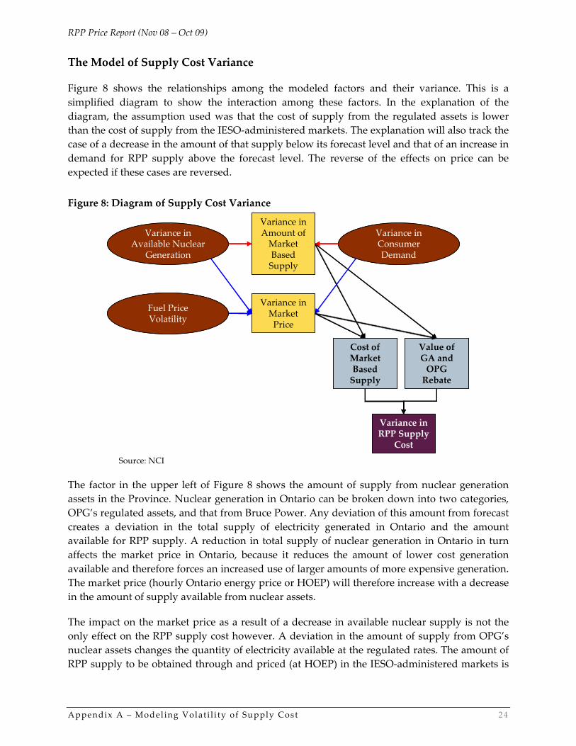
The Model of Supply Cost Variance
Figure 8 shows the relationships among the modeled factors and their variance. This is a simplified diagram to show the interaction among these factors. In the explanation of the diagram, the assumption used was that the cost of supply from the regulated assets is lower than the cost of supply from the IESO‐administered markets. The explanation will also track the case of a decrease in the amount of that supply below its forecast level and that of an increase in demand for RPP supply above the forecast level. The reverse of the effects on price can be expected if these cases are reversed.
Figure 8: Diagram of Supply Cost Variance
Variance in Available Nuclear
Generation
Variance in Consumer Demand
Fuel Price Volatility
Variance in Amount of Market Based Supply
Variance in Market Price
Cost of Market Based Supply
Value of GA and OPG Rebate
Variance in RPP Supply
Cost
Variance in Available Nuclear
Generation
Variance in Consumer Demand
Fuel Price Volatility
Variance in Amount of Market Based Supply
Variance in Market Price
Cost of Market Based Supply
Value of GA and OPG Rebate
Variance in RPP Supply
Cost Source: NCI
The factor in the upper left of Figure 8 shows the amount of supply from nuclear generation assets in the Province. Nuclear generation in Ontario can be broken down into two categories, OPG’s regulated assets, and that from Bruce Power. Any deviation of this amount from forecast creates a deviation in the total supply of electricity generated in Ontario and the amount available for RPP supply. A reduction in total supply of nuclear generation in Ontario in turn affects the market price in Ontario, because it reduces the amount of lower cost generation available and therefore forces an increased use of larger amounts of more expensive generation. The market price (hourly Ontario energy price or HOEP) will therefore increase with a decrease in the amount of supply available from nuclear assets.
The impact on the market price as a result of a decrease in available nuclear supply is not the only effect on the RPP supply cost however. A deviation in the amount of supply from OPG’s nuclear assets changes the quantity of electricity available at the regulated rates. The amount of RPP supply to be obtained through and priced (at HOEP) in the IESO‐administered markets is

RPP Price Report (Nov 08 – Oct 09)
Appendix A – Model ing Volat i l i ty of Supply Cost 25
the residual of the demand after the supply from the regulated assets, NUG contracts, and any contracts the OPA has entered into with generators. A decrease in the supply from OPG’s nuclear assets will therefore increase the amount to be obtained in the market. Since the regulated price of electricity from OPG’s nuclear assets is expected, at most times, to be lower than HOEP, a decrease in supply available from the regulated assets will increase the RPP supply cost. This is not necessarily the case for variations in the amount of supply from Bruce Power’s nuclear assets. The contract price for output from Bruce A is higher than the regulated rate for OPG, hence there may be periods when supply receiving market prices is less expensive than supply from Bruce.
The upper right hand side of Figure 8 shows a similar situation for variances from expected demand. As with a change in supply, this affects RPP supply costs in two ways. An increase in demand produces an increase in the amount of supply that is required for the RPP consumers, and therefore a change in the amount that must be obtained and priced in the IESO‐administered markets. A deviation in demand from forecast amounts also changes the supply and demand situation in the IESO‐administered markets and affects prices.
Volatility in fuel prices also has a significant impact on market prices, and hence the RPP supply cost. This is shown in the lower left hand corner of Figure 8. The price of natural gas is by far the most volatile of the prices for the various fuels used to generate electricity in the IESO administered market. While coal‐fired generation in Ontario is currently the predominant marginal resource, natural gas fired generation typically sets the price during the hours of highest demand. It is during these hours that supply is the tightest, and vulnerability to a single fuel source is at its highest.
It is understood that these are not the only factors that influence the RPP supply cost. They do however account for the most significant portion of the risk. Taking into account additional sources of variance adds significant complexity to the modelling process and would only be expected to provide marginal value.
Simulating the Model
A combination of statistical and econometric techniques was used to model this system and produce a distribution for the variance of RPP supply costs.
The basic methodology used was a Monte Carlo technique. Such techniques make a large number of simulations of a complex system where each of several input variables is subject to random factors that can be described by a probability distribution. The model simulates the system by taking a large number of random draws from the distributions of each of the variables subject to random factors. Each draw produces a value of the variable to be used as input to the model.

RPP Price Report (Nov 08 – Oct 09)
Appendix A – Model ing Volat i l i ty of Supply Cost 26
Deriving Probability Distributions
The first steps were to estimate probability distributions for the three key factors: supply from nuclear assets, demand from Ontario consumers, and the volatility of natural gas prices.
To estimate nuclear supply probabilities, Navigant Consulting used available information and modeling assumptions about forced and unforced outage rates. Since Navigant Consulting’s existing forecast of nuclear supply, and therefore of total Ontario supply, already models random forced outages, probabilities were chosen that represented extreme outage situations that are not captured in the ProSym model.
The major factor causing day‐to‐day variance in customer demand is weather. The most important weather factor is temperature. In the winter, colder weather means more electricity is used for space heating, and in the summer, warmer weather means more electricity is used for air conditioning. From historical weather data for 20 years, a historical frequency distribution of temperature was computed. This historical frequency distribution was then utilized as the (assumed normal) probability distribution of temperature.
To calculate the effect of weather on demand, data published by the IESO on the sensitivity of Ontario load to weather was used. These data show the effect of degree days on total Ontario load. The weather data provided a distribution of weather, and the translation through the IESO information provided a distribution of demand. The IESO data shows the effect of weather on load for the entire system. Electricity demand from eligible RPP consumers is likely to be more sensitive to weather than Ontario demand as a whole, because industrial load (which is not eligible for the RPP) is not very responsive to weather. In modeling the variance, 80% of the weather impact was therefore allocated in the winter to the RPP consumers; in summer, 60% was allocated. The difference in attribution reflects the fact that large commercial consumers which are not eligible for the RPP are very likely to have air conditioning, and therefore have load that is sensitive to increases in temperature, but are not very likely to have electric space heating.
Finally, a probability distribution for the volatility of natural gas prices was derived. The natural gas prices used to develop the parameters for the distribution were taken from historical Henry Hub prices. Henry Hub has the most robust and complete historical data available (basis differential were used to convert these gas prices to Dawn Hub natural gas prices for forecasted values). Data from January 1990 through August 2007 was analyzed to develop the descriptive statistics.
The sensitivity of Ontario electricity prices to a change in natural gas prices was determined through simulation of the Ontario wholesale electricity production‐cost model under both a high and low gas price scenarios.23
23 The results of the high / low gas price sensitivity are provided in the Navigant Consulting Ontario Wholesale Electricity Market Price Forecast Report.

RPP Price Report (Nov 08 – Oct 09)
Appendix A – Model ing Volat i l i ty of Supply Cost 27
The Supply / Demand Effect on Market Price
The diagram (Figure 8) and the above discussion indicate that a change in supply or demand conditions can be expected to have an impact on RPP supply cost in two ways: through the impact on the fraction of supply to be priced in the IESO‐administered markets and through the price in those markets. The impact of the supply amount can be calculated directly. The impact on the market price must be estimated.
For that estimation, Navigant Consulting used econometric techniques. A single‐equation regression model for the HOEP was constructed, with electricity demand and supply, and natural gas prices in Ontario as the independent variables. The resulting equation fit the data reasonably well. The coefficients of the independent variables were all highly significant and had the expected signs. The equation explained about 60% of the historical variance in the HOEP.
Computing RPP Supply Cost
All of these elements together then allowed calculation of the variance of the RPP supply cost from its expected level. For this calculation, as mentioned, a random simulation (Monte Carlo) technique was used, under which independent draws from each of the three probability distributions were made.
Each set of random draws sampled from the three probability distributions was used to obtain values of supply from the nuclear assets, weather conditions, and natural gas prices. Weather conditions were translated into demand impacts, using the information from the IESO. The supply and demand conditions were then translated into a market price, using the structure of the estimated equation. Natural gas price conditions were translated into a market price using the sensitivity terms obtained from the static price forecast.
The variance of the RPP supply cost was then calculated by comparing the RPP supply cost calculated using the static forecast values to the values calculated from the conditions under each of the random draws.
Variance Results
Figure 9 shows the cumulative variance over the entire year for all 5000 simulations. The majority of simulations (roughly 3000 of the 5000) have negative variances; that is, they generate variances that consumers will later have to pay. Also shown on this chart are the approximate locations of the variance simulations chosen to represent the 10th, 25th, 50th, 75th, and 90th percentiles.

RPP Price Report (Nov 08 – Oct 09)
Appendix A – Model ing Volat i l i ty of Supply Cost 28
Figure 9: Cumulative Variances over Entire Term
‐$1,200
‐$900
‐$600
‐$300
$0
$300
$600
$900
$1,200
0% 10% 20% 30% 40% 50% 60% 70% 80% 90% 100%Percentile
Cum
ulative Net Variance ($ million)
‐$2,500
‐$1,500
‐$500
$500
$1,500
0% 20% 40% 60% 80% 100%
10th
Percentile
25th
Percentile
Median
75th
Percentile
90th
Percentile
Source: NCI
The median variance, which represents the adjustment that will be applied to the RPA, was found to be negative $57 million. The inclusion of this adjustment factor in the total RPP supply cost means that there is an equal likelihood of either a consumer credit variance or a consumer debit variance at the end of the RPP year. This adjustment factor is referred to as the stochastic adjustment in the body of this report.