Regularized Mixture Density Estimation With an Analytical Setting of Shrinkage Intensities

460 IEEE TRANSACTIONS ON NEURAL NETWORKS AND LEARNING SYSTEMS, VOL. 24, NO. 3, MARCH 2013

Regularized Mixture Density Estimation With anAnalytical Setting of Shrinkage Intensities

Zohar Halbe, Maria Bortman, and Mayer Aladjem, Member, IEEE

Abstract— In this paper, we propose a method for P-variateprobability density estimation assuming a Gaussian mixturemodel (GMM). Our method exploits a regularization techniquefor improving the estimation accuracy of the GMM componentcovariance matrices. We derive an expectation maximizationalgorithm for fitting our regularized GMM (RGMM), whichexploits an analytical Ledoit–Wolf-type shrinkage estimation ofthe covariance matrices. Our method is compared with recentmodel-based and variational Bayes approximation methods usingsynthetic and real data sets. The obtained results show that theproposed RGMM method achieves a significant improvement inthe performance of multivariate probability density estimationwith respect to other methods on both the synthetic and the realdata sets.

Index Terms— Expectation maximization (EM) algorithm,Gaussian mixture model (GMM), model selection, multivariatedensity estimation, regularization, shrinkage estimation.

I. INTRODUCTION

IN THIS paper the problem of modeling a P-variate prob-ability density function f (x)(x ∈ R P ) on the basis of a

training setX = {x1, x2, . . . , xN } (1)

is considered. Here xn ∈ R P (n = 1, . . . , N) are dataobservations drawn from the underlying density. We assume aGaussian mixture model (GMM) [1], [2] for f (x)

f (x) =M∑

j=1

π j�� j

(x − μ j

)(2)

where, M denotes the number of the Gaussian components(clusters), π j are mixing coefficients, which are nonnegativeand sum to one and �� j (x − μ j ) denotes P-variate normaldensity with mean vector μ j and covariance matrix � j . TheGMM (2) is widely applied due to its ease of interpretationby viewing each fitted Gaussian component as a distinctcluster in the data. The clusters are centered at the means μ jand have geometric features (shape, volume, and orientation)determined by the covariance matrices � j . In addition, theGMM enables us to approximate any continuous density toarbitrary accuracy [3].

Manuscript received June 1, 2012; revised November 21, 2012; acceptedNovember 23, 2012. Date of publication January 14, 2013; date of currentversion January 30, 2013.

The authors are with the Department of Electrical and Computer Engineer-ing, Ben-Gurion University of the Negev, Beer-Sheva 84105, Israel (e-mail:[email protected]; [email protected]; [email protected]).

Digital Object Identifier 10.1109/TNNLS.2012.2234477

The problem of determining the number M and the para-meterization of � j in f (x) (2) is known as model selection.Usually [4, Ch. 7], several models are considered and anappropriate one is chosen using a model selection criterion.Some popular criteria are Akaike information criterion [5],Bayesian information criterion (BIC) [6], normalized entropycriterion (NEC) [7], [8], integrated classification likelihood[9], Monte–Carlo cross validation (MCCV) [10], minimummessage length [11], and deviance information criterion (DIC)[12], [13]. Another strategy for model selection is the vari-ational Bayes (VB) approximation approach [1, Ch. 9],[14]–[16] which treats the adjustable parameters as randomvariables by introducing priors for them. VB approxima-tion methods overcome intractable integrals which appear inBayesian model selection methods [1, Ch. 10], by consideringfactorization assumptions. Ghahramani and Beal [15] havedeveloped a VB approximation method for estimation multi-variate density modeled by a mixture of factor analysers (FA).We refer to the latter method as VBMFA. Constantinopoulosand Likas [17] have proposed an incremental VB updatingsplitting procedure (named VBgmmSplit) for computing Mand � j in f (x) (2). The latter procedure was modifiedrecently [18] for accelerating the convergence of the incremen-tal splitting of the Gaussian components. In [19] a variationalapproximation of DIC was proposed, which avoids a computa-tionally demanding Markov chain Monte Carlo procedure usedin the original DIC [12], [13]. In our experiments (Section III),we employed BIC [6], NEC [8], MCCV [10], VBMFA [15]and VBgmmSplit [17] model selection methods.

Conventional GMMs [2], [3], use three types of � j inf (x) (2), namely full (unrestricted) (� j = F j ), diagonal(� j = D j ) or spherical (� j = S j ) parameterizations ofthe covariance matrices, where F j denotes a positive defi-nite symmetric matrix; D j a diagonal matrix having positivediagonal elements and S j a diagonal matrix having equalpositive diagonal elements. For a predefined number M and aparameterization � j = S j , D j or F j , the values of π j , μ j ,and � j in f (x) (2) are determined by an expectation maxi-mization (EM) algorithm [20, Ch. 3], [21], which maximizesthe likelihood of the parameters to the training set. The EMalgorithm performs poorly for a small ratio

(N j /P

)of the

number N j of the points in the j th cluster and the dimensionP of the points. This is more pronounced for the parame-terization � j = F j having a large number (P(P + 1)/2)of adjustable parameters, which results in highly variableF j (smallest eigenvalues are underestimated and largest ones

2162–237X/$31.00 © 2013 IEEE

HALBE et al.: REGULARIZED MIXTURE DENSITY ESTIMATION 461

are overestimated) [22, p. 1174]. In the EM algorithm, theinversion of � j is needed, which is numerically ill-conditionedfor � j = F j and a small size of the training set [23, p. 366].Ormoneit and Tresp [24] have shown that some problemscaused by the ill-conditioned F j can be handled by bagging,penalized likelihood and Bayesian estimation techniques. Ina scenario of small size of the training set, the conventionalGMMs use the simple parameterization � j = S j or D j inorder to overcome computational instability of the EM algo-rithm for � j = F j Unfortunately the latter parameterizationscould be highly biased estimators of the real covariancematrices.

Fraley and Raftery [25], [26] have proposed a model-basedGMM (MbGMM)1 for density estimation, which extends theconventional GMMs by employing an enlarged set of theparameterizations for � j in f (x) (2). For some of themthe number of the adjustable parameters has been reducedsignificantly while the flexibility with respect to restrictedconventional parameterizations S j and D j is increased.

In [27]–[29] regularized GMMs (RGMMs) have been devel-oped, which could be viewed as a continuous extension of theMbGMM. RGMMs shrink the maximum likelihood estimatorof � j to suitable chosen restricted parameterizations. In theseworks, the values of the shrinkage intensities, which reflectthe appropriate contribution of each type of parameterization,are computed by a cross-validation (CV) procedure on a meshfor the values of the intensities. The CV is a computationally-intensive procedure, which needs preliminary study for settinga suitable scale of the mesh, can be applied to a limited numberof the intensities. The latter forces the authors of [27]–[29]to employ equal values of the intensities for all componentcovariance matrices into the RGMMs.

In this paper we propose a method for P-variate probabilitydensity function estimation by means of RGMM with ananalytical setting of shrinkage intensities. In Section II, wederive explicit formulas for computing the shrinkage inten-sities for our RGMM by employing the analytical shrinkagetheory of Ledoit and Wolf (LW) [23], [30]. To the best ofour knowledge, these formulas (derived in Section II-B2) donot appear in the literature and are derived for the first timein this paper. In addition, the EM algorithm, proposed inSection II, makes it possible to compute specific shrinkageintensities for the covariance matrices into our RGMM, whichwas not possible previously [27]–[29]. Section III presentscomparative studies of our method with conventional GMMs,MbGMM, VBMFA, and VBgmmSplit methods on syntheticand real data sets. In addition, in Section III, the propersetting of the values of shrinkage intensities by the derivedformulas and the reasonable computation complexity of ourRGMM are confirmed experimentally. The obtained resultsshow that our method is an attractive choice for GMM densityestimation. Section IV summarizes some recent developmentsin the shrinkage estimation of the covariance matrix [31]–[37]which we intend to study and employ in future research.

1The software toolbox which implements the MbGMM [25], [26] is knownas MCLUST and is available in http://www.stat.washington.edu/mclust/.

II. RGMM WITH AN ANALYTICAL SETTING OF

SHRINKAGE INTENSITIES

In this paper, we model a P-variate probability densityfunction by means of a RGMM

f (R)(x) =M(R)∑

j=1

π(R)j �� j (α j , β j )(x − μ

(R)j ) (3)

for

� j (α j , β j ) = β j [α j S j + (1 − α j )D j ] + (1 − β j )F j , (4)

α j , β j ∈ [0, 1].

In (4), � j (α j , β j ) is a P × P regularized sample covariancematrix and α j , β j are shrinkage intensities. The valueof α j controls the migration of the spherical componentcovariance matrices S j toward diagonal matrices D j . Thevalue α j = 1 gives rise to S j , whereas α j = 0 yields D j .Values between these limits compromise between S j and D j .For a given value of α j , the intensity β j controls the degreeof the approach to the unrestricted covariance matrix F j .The estimator � j (α j , β j ) (4) implies a rich class ofalternatives to the conventional parameterizations of the GMMcomponent covariance matrices, compromising between thesimple parameterizations S j and D j having a small number ofparameters (one and P , respectively) and the most complicated(unrestricted) parameterization F j having the largest number(P(P + 1)/2) of parameters. It must be noted that (4) isclosely related to and stimulated by the regularization of thesample covariance matrices proposed by Friedman [38].

In this paper, we assume that the training observations xn ,n = 1, 2, . . . , N , in X (1) are independent and identicallydistributed. Taking a generative point of view [20, Ch. 3], welook at each data point xn as generated by a specific Gaussiancomponent �� j (α j , β j )(x − μ

(R)j ). The latter results in adding

“missing data” Z = {z1, z2, . . . , zN }, which comprises indi-cator vectors zn = [

zn1, zn2, . . . , znM(R)

]T −znj = 1 for xn

drawn from �� j (α j , β j )(x − μ(R)j ) otherwise znj = 0. In the

following explanation, we refer to {X, Z} as complete dataand denote by f (R)(xn, zn| θ1, θ2) the joint distribution ofxn and zn having adjustable parameters

θ1 ={π

(R)j , μ

(R)j , S j , D j , F j

} M (R)

j=1(5)

θ2 ={α j , β j

} M (R)

j=1(6)

where π(R)1 , . . . , π

(R)

M(R) are the categorical probabilities of themultinomial distribution of znj .

In the remaining part of this section, an EM algorithmfor computing the appropriate values of θ1 (5) and θ2 (6) isderived. Our algorithm makes it possible to calculate specificshrinkage intensities θ2 = { α j , β j } for each � j (α j , β j )in f (R) (x) (3), which was not possible previously [27]–[29].In the following Sections II-A and II-B the expectation-step(E-step) and the maximization-step (M-step) of the EM algo-rithm are explained. The last Section II-C summarizes theproposed algorithm.


A. E-Step

In the following explanation, we mark by the symbol hat (^)the values of θ1 (5) and θ2 (6) calculated by the algorithm andadd a superscript i to θ1, θ2 and their values for indicating theiteration. Using these notations, following the classical E-step[20, Ch. 3], we compute:

γ(i)nj =

π(R)(i)j �

(i)

�(i)j (α(i)

j , β(i)j )

(xn − μ(R) (i)j )

∑M(R)

j=1 π(R)(i)j �

(i)

�(i)j (α(i)

j , β(i)j )

(xn − μ(R) (i)j )

(7)

which is the probability of responsibility [1, Ch. 9.2] of thej th component �

�(i)j (α

(i)j , β

(i)j )

(x − μ(R) (i)j ) in f (R) (x) (3) for

generating data point xn . The right-hand side in (7) is obtainedby expectation (EZ|X, θ

(i)1 , θ

(i)2

{znj

}) of the indicator variable

znj under the conditional distribution f (R)(zn | xn, θ(i)1 , θ

(i)2 )

for the values θ(i)1 = { π

(R)(i)j , μ

(R)(i)j , S

(i)j , D

(i)j , F

(i)j } M (R)

j=1

and θ(i)2 = {α(i)

j , β(i)j }M(R)

j=1 at the step i .

B. M-Step

In this section a specific M-step for the EM algorithmis derived. As in [20, Ch. 3] and [39], first we write theexpression of the log-likelihood function of the complete data{X, Z} at step i

ln f (R)(

X, Z| θ(i)1 , θ

(i)2

)= ln

N∏

n=1

f (R)(

xn, zn| θ(i)1 , θ

(i)2

)

=N∑

n=1

M(R)∑

j=1

znj ln

[π

(R)(i)j �

�(i)j

(α

(i)j , β

(i)j

)(xn −μ(R)(i)j

)]. (8)

Then we obtain the expectation of ln f (R)(X, Z| θ(i)1 , θ

(i)2 )

over Z for given X and values θ(i−1)

1 , θ(i−1)

2 computed in theprevious iteration i − 1

Q(θ

(i)1 , θ

(i)2 ; θ

(i−1)

1 , θ(i−1)

2

)

= EZ|X, θ

(i−1)1 , θ

(i−1)2

{ln f (R)

(X, Z| θ

(i)1 , θ

(i)2

) }

=M(R)∑

j=1

N (i)j lnπ

(R) (i)j − 1

2

[P N (i)

j ln(2π)

+N (i)j ln

∣∣∣�(i)j

(α

(i)j , β

(i)j

)∣∣∣+tr(

W (i)j �

(i)−1

j

(α

(i)j , β

(i)j

))].

(9)

Here �(i)−1

j (α(i)j , β

(i)j ) indicates the matrix inversion, tr(·)

denotes the trace operator, | · | indicates determinant of thematrix and the matrix W(i)

j is given by

W(i)j =

N∑

n=1

γ(i−1)n j

(xn − μ

(R) (i)j

)(xn − μ

(R) (i)j

)T(10)

for

μ(R)(i)j =

∑Nn=1 γ

(i−1)n j xn

N (i)j

(11)

N (i)j =

N∑

n=1

γ(i−1)n j (12)

where γ(i−1)n j is computed by (7) at the previous step i − 1.

Our M-step comprises two parts. In the first part,

explained in Section II-B1, we compute θ(i)1 = { π

(R)(i)j ,

μ(R)(i)j , S

(i)j , D(i)

j , F(i)j } M (R)

j=1 , which maximizes conventional

EM lower bounds of Q(θ (i)1 , θ2; θ

(i−1)

1 , θ(i−1)

2 ) (9) for θ2 =θ

F2 = { ·, β j = 0} M (R)

j=1 , θ2 = θD2 = { α j = 0, β j = 1} M (R)

j=1

and θ2 = θS2 = { α j = 1, β j = 1} M (R)

j=1 . Then in the second

part of our M-step (Section II-B2), after having found θ(i)1 we

calculate θ(i)2 = {α(i)

j , β(i)j }M(R)

j=1 , giving rise to �(i)j (α(i)

j , β(i)j ),

which is most similar (in the sense of Ledoit and Wolf [23])to the unobservable (true) component covariance matrices ofthe RGMM (3) at step i .

1) Computation θ(i)1 Which Maximizes Conventional EM

Lower Bounds of the Expected Complete Data Log-Likelihood

Function Q(θ (i)1 , θ2; θ

(i−1)

1 , θ(i−1)

2 ) (9): The conventional

EM lower bounds of Q(θ (i)1 , θ2; θ

(i−1)

1 , θ(i−1)

2 ) (9) are

[20, Ch. 3] for θ2 = θF2 = { ·, β j = 0} M (R)

j=1 (GMM havingfull component covariance matrices)

Q(θ

(i)1 , θ

F2; θ

(i−1)

1 , θ(i−1)

2

)=

M(R)∑

j=1

N (i)j

[ln π

(R) (i)j

−1

2

[P ln(2π) + ln |F(i)

j | + 1

N (i)j

tr(W(i)j F(i)−1

j )

]](13)

for θ2 = θD2 = { α j = 0, β j = 1} M (R)

j=1 (GMM havingdiagonal component covariance matrices)

Q(θ

(i)1 , θ

D2 ; θ

(i−1)

1 , θ(i−1)

2

)=

M(R)∑

j=1

N (i)j

[ln π

(i) (R)j

−1

2

[P ln(2π) + ln |D(i)

j | + 1

N (i)j

tr(W(i)j D(i)−1

j )

]](14)

and for θ2 = θS2 = { α j = 1, β j = 1} M (R)

j=1 (GMM havingspherical component covariance matrices)

Q(θ

(i)1 , θ

S2; θ

(i−1)

1 , θ(i−1)

2

)=

M(R)∑

j=1

N (i)j

[ln π

(R) (i)j

−1

2

[P ln(2π) + ln |S(i)

j | + 1

N (i)j

tr(W(i)j S(i)−1

j )

]]. (15)

The stationary points θ(i)1 = { π

(R)(i)j , μ

(R)(i)j , S(i)

j , D(i)j ,

F(i)j } M (R)

j=1 of the lower bounds (13)–(15) are computed by the


Fig. 1. Illustration the solution θ(i)1 =

{π

(R)(i)j , μ

(R)(i)j , S(i)

j , D(i)j ,

F(i)j

}M(R)

j=1(16)–(19).

following expressions [20, Ch. 3] μ(R)(i)j is obtained by (11)

and

π(R) (i)j = 1

N

N∑

n=1

γ(i−1)n j (16)

S(i)j = 1

P N (i)j

tr(W(i)j ) I (17)

D(i)j = 1

N (i)j

diag(W(i)j ) (18)

F(i)j = 1

N (i)j

W(i)j (19)

for γ(i−1)n j computed by (7) at the previous step i −1, and N (i)

j ,

W(i)j are calculated by (12) and (10), respectively. In (17), I is

the identity matrix and in (18) diag(W(i)j ) denotes the matrix

having the diagonal entries of W(i)j .

Fig. 1 illustrates that the solution θ(i)1 = {π (R)(i)

j , μ(R)(i)j ,

S(i)j , D(i)

j , F(i)j } M (R)

j=1 (16)–(19) is composed of the sta-

tionary points of Q(θ (i)1 , θ

F2; θ

(i−1)

1 , θ(i−1)

2 ) (13), Q(θ (i)1 ,

θD2 ; θ

(i−1)

1 , θ(i−1)

2 ) (14) and Q(θ (i)1 , θ

S2; θ

(i−1)

1 , θ(i−1)

2 ) (15)(the conventional EM lower bounds for GMMs having unre-stricted (full), diagonal and spherical component covari-

ance matrices). By freezing θ(i−1)

2 and iterating our E- and

M-steps we will approach the stationary point θ(i)∗1

of the conditional likelihood functions Q(θ(i)1 , θ2; θ

(i−1)

1 ,

θ(i−1)

2 ) (9) for θ2 = θF2 = {·, β j = 0}M(R)

j=1 , θ2 = θD2 =

{α j = 0, β j = 1}M (R)

j=1 , θ2 = θS2 = { α j = 1, β j = 1} M (R)

j=1 .In a preliminary experimental study of our method we didnot find any loss of accuracy in neglecting the computation

of θ(i)∗1 and using θ

(i)1 in the iterations. The latter observation

is not surprising because the goal of our method is not to

find the current local minimum at θ(i)∗1 but to compute θ

(i)2 =

{α(i)j , β

(i)j }M(R)

j=1 , giving rise to �(i)j (α(i)

j , β(i)j ) which are most

similar (in the sense of LW [23]) to the unobservable (true)component covariance matrices of the current model (see nextSection II-B2).

Fig. 2. Illustration the computations of θ(i)1 (5) and θ

(i)2 (6) in our M-step.

Fig. 2 illustrates the computations of the values of θ1(5) and θ2 (6) in the i th iteration of our M-step. We showschematically the expected complete data log-likelihood Q(·)(9) as a function of θ1 (5) and θ2 (6). The left slice in

this figure presents the solution θ(i)1 (16)–(19). In more detail

the latter was illustrated in Fig. 1. Here, for simplicity of

illustration, Q(θ (i)1 , θ2; θ

(i−1)

1 , θ(i−1)

2 ) (9) is presented for

different θ2 = θF2 = { ·, β j = 0} M (R)

j=1 , θ2 = θD2 = { α j = 0,

β j = 1} M (R)

j=1 and θ2 = θS2 = { α j = 1, β j = 1} M (R)

j=1 as asingle narrow surface and the conventional EM lower bounds

Q(θ (i)1 , θ2; θ

(i−1)

1 , θ(i−1)

2 ) (13)–(15) are combined into asingle arc. Into the left slice the solid lines with arrows indicate

the flow of the computations of θ(i)1 (16)–(19). The calculation

starts from point (θ(i−1)

1 , θ(i−1)

2 ) computed at previous (i−1)th

iteration. The value θ(i−1)

2 = {α(i−1)j , β

(i−1)j }M(R)

j=1 was used for

the calculation of γ(i−1)n j by (7), which is kept unchanged in the

expressions of θ(i)1 (16)–(19). The latter is illustrated in Fig. 2

by the path of the arrows into the left slice. After reaching the

destination (θ(i)1 , θ

(i−1)

2 ) we keep θ(i)1 unchanged and compute

θ(i)2 = {α(i)

j , β(i)j }M(R)

j=1 , which gives rise to �(i)j (α

(i)j , β

(i)j )

(4) which is most similar (in the sense of LW [23]) tothe unobservable (true) component covariance matrix of thecurrent model. In Fig. 2 the latter is illustrated by a horizontal

arrow from point (θ(i)1 , θ

(i−1)

2 ) to point (θ(i)1 , θ

(i)2 ), which is

the starting point of the iteration (i + 1) in our algorithm.

The computation of θ(i)2 = {α(i)

j , β(i)j }M(R)

j=1 is explained in thefollowing section.

2) Computation θ(i)2 = {α(i)

j , β(i)j }M(R)

j=1 Giving Rise to

�(i)j (α

(i)j , β

(i)j ), Most Similar to the True Component Covari-

ance Matrices of the Current Model: Here, following LW ana-lytic shrinkage [23], we derive explicit formulas for computing

shrinkage intensities (α(i)j , β

(i)j ), giving rise to �

(i)j (α

(i)j , β

(i)j ),

which is most similar to the unobservable true componentcovariance matrices K(i)

j of the current model. To the bestof our knowledge, the formulas in this section do not appearin the literature and are derived for the first time in this paper.


As in [23] the LW-criterion is minimized

L(i)j (α j , β j ) = E

{∥∥∥�(i)j (α j , β j ) − K(i)

j

∥∥∥2

F

}

=P∑

l=1

P∑

m=1

E{

[σ (i)j lm(α j , β j ) − k(i)

j lm]2}(20)

for{α j , β j : 0 ≤ α j ≤ 1; 0 ≤ β j ≤ 1}. (21)

In LW-criterion (20), ‖ · ‖2F denotes the squared Frobenius

norm [40]; k(i)j lm and σ

(i)j lm(α j , β j ) are the entries of K(i)

j and

�(i)j (α j , β j ) respectively. Using that F(i)

j (19) is unbiased

estimator of K(i)j (K(i)

j = E{F(i)j }) and after some algebraic

manipulations of the right-hand side of (20) the criterionL(i)

j (α j , β j ) can be re-written in the following form:

L(i)j (α j , β j ) =

P∑

l=1

P∑

m=1

[α2

j β2j var

{s(i)

j lm

}

+ β2j (1 − α j )

2 var{d(i)

j lm

}

+ 2(α j − α2j )β

2j cov

{s(i)

j lm, d(i)j lm

}

+ (1 − β j )2 var{ f (i)

j lm}+ 2α j (β j − β2

j ) cov{s(i)

j lm , f (i)j lm

}

+ 2(1 − α j )(β j − β2j ) cov

{d(i)

j lm, f (i)j lm

}

+ [α jβ j E{s(i)j lm} + β j (1 − α j )E

{d(i)

j lm

}

− β j E{ f (i)j lm}]2] (22)

where s(i)j lm , d(i)

j lm, and f (i)j lm are the entries of the

matrices S(i)j (17), D(i)

j (18) and F(i)j (19) respectively, and

var{·} and cov{·, ·} denote the variance and covariance ofthe entries. Using auxiliary variable δ j = α j β j in (22) weobtain L(i)

j (δ j , β j ) in the form of a quadratic function havinga unique stationary point

α∗(i)j =

∑Pl=1

∑Pm=1

[cov

{d(i)

jlm , f (i)jlm

}−cov{s(i)jlm , f (i)

jlm}]

β∗(i)j

∑Pl=1

∑Pm=1

[var

{s(i)jlm

} + var{d(i)jlm

}−2 cov{s(i)jlm , d(i)

jlm}+

(E

{d(i)

jlm} − E

{s(i)jlm

})2]

(23)

β∗(i)j =

∑Pl=1

∑Pm=1

[var

{f (i)l jm

}−cov{d(i)

jlm , f (i)jlm

}]

∑Pl=1

∑Pm=1

[var

{d(i)

jlm}+var

{f (i)l jm

}−2 cov{d(i)

jlm , f (i)jlm

}+(

E{

f (i)jlm

}−E{d(i)

jlm})2

] .

(24)

The point (α∗(i)j , β

∗(i)j ) (23), (24) may exceed the boundaries

(21) and in this case the minimal value of L(i)j (α j , β j ) (20)

must be computed [41, Ch. 6] on the edges of the region (21),which gives: for the edge α

∗(i)j = 0 (illustrated as dashed

vertical line at α j = 0 in Fig. 3)

β∗(α

∗(i)j =0)

j = arg minβ j

E

{ ∥∥∥β j D(i)j + (1 − β j )F

(i)j − K(i)

j

∥∥∥2

F

}

=∑P

l=1∑P

m=1

[var

{f (i)jlm

} − cov{d(i)

jlm , f (i)jlm

}]

∑Pl=1

∑Pm=1

[var

{d(i)

jlm} + var

{f (i)jlm

} − 2 cov{d(i)

jlm , f (i)jlm

} +(

E{

f (i)jlm

} − E{d(i)

jlm})2

]

(25)

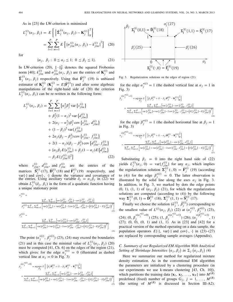
Fig. 3. Regularization solutions on the edges of region (21).

for the edge α∗(i)j = 1 (the dashed vertical line at α j = 1 in

Fig. 3)

β∗(α

∗(i)j =1)

j = arg minβ j

E

{ ∥∥∥β j S(i)j + (1 − β j )F(i)

j − K(i)j

∥∥∥2

F

}

=∑P

l=1∑P

m=1

[var

{f (i)jlm

}−cov{s(i)jlm , f (i)

jlm}]

∑Pl=1

∑Pm=1

[var

{s(i)jlm

}+var{

f (i)jlm

}−2 cov{s(i)jlm , f (i)

jlm}+

(E

{f (i)jlm

}−E{s(i)jlm

})2]

(26)

for the edge β∗(i)j = 1 (the dashed horizontal line at β j = 1

in Fig. 3)

α∗(β

∗(i)j =1)

j = arg minα j

E

{ ∥∥∥α j S(i)j + (1 − α j )D(i)

j − K(i)j

∥∥∥2

F

}

=∑P

l=1∑P

m=1

[var

{d(i)

jlm} − cov

{s(i)jlm , d(i)

jlm}]

∑Pl=1

∑Pm=1

[var

{s(i)jlm

} + var{d(i)

jlm} − 2 cov

{s(i)jlm , d(i)

jlm} +

(E

{d(i)

jlm} − E

{s(i)jlm

})2] .

(27)

Substituting β j = 0 into the right hand side of (22)yields L(i)

j (α j , 0) = var{ f (i)j lm} for any α j , which implies

the regularization solution �(i)j (·, 0) = F(i)

j (19) (according

to (4)) for the edge β∗(i)j = 0. The latter observation is

illustrated by the solid line along the axes α j in Fig. 3.In addition, in Fig. 3, we marked by dots the edge points(0, 1), (1, 1) of (α j , β j ) (21), for which the regularizationsolutions are computed (according to (4)) by the followingway �

(i)j (0, 1) = D(i)

j (18), �(i)j (1, 1) = S(i)

j (17).

Finally we choose the solution (α(i)j , β

(i)j ) corresponding to

the smallest value of L(i)(α j , β j ) (22) at (α∗(i)j , β

∗(i)j ) (23),

(24); (0, β∗(α

∗(i)j =0)

j ) (25); (1, β∗(α

∗(i)j =1)

j ) (26); (α∗(β

∗(i)j =1)

j , 1)(27); (0, 0), (0, 1) and (1, 1). As in [23] and [42] for apractical version of the method operating on a data sample, thepopulation operators E{·}, var{·} and cov{·, ·} in (23)–(27)are replaced by corresponding sample averages (Appendix).

C. Summary of our Regularized EM Algorithm With AnalyticalSetting of Shrinkage Intensities

(α j , β j

)in � j

(α j , β j

)(4)

Here we summarize our method for regularized mixturedensity estimation. As in the conventional EM algorithmthe parameters are initialized by a clustering procedure (inour experiments we use k-means clustering [43, Ch. 10]),which partitions the training data {x1, x2, . . . , xN } into M(R)

predefined (fixed) number of groups G j , j = 1, . . . , M(R)

(the setting of M(R) is discussed in Section III-A2).


An indicator vector zn = {zn1, zn2, . . . , znM(R) } is

associated with each observation xn in the following way. Forxn ∈ G j , zn j = 1, otherwise zn j = 0 for n = 1, . . . , Nand j = 1, . . . , M(R). Starting with i = 1 and settingγ

(1)nj = znj the M-step (Section II-B) and the E-step

(Section II-A) are iterated until the convergence criterion[20, Ch. 3] is satisfied.

M-Step (Section II-B): Using expressions derived inSection II-B we compute μ

(R)(i)j (11); N (i)

j (12); π(R)(i)j (16);

W(i)j (10); S(i)

j (17); D(i)j (18); F(i)

j (19). Then �(i)j (α(i)

j , β(i)j )

= β(i)j [α(i)

j S(i)j + (1 − α

(i)j )D(i)

j ] + (1 − β(i)j )F(i)

j is calculated

for the values (α(i)j , β

(i)j ) obtained by the procedure explained

in Section II-B2.E-Step (Section II-A): The value of γ

(i)nj is computed by (7).

III. EXPERIMENTS

Here, the proposed RGMM method (Section II) for densityestimation is compared with conventional GMMs [20, Ch. 3],MbGMMs [25], VBMFAs [15] and VBgmmSplit [17]methods. Section III-A presents the comparisons on syntheticdata sets. In addition, in this section the proper setting ofthe values of shrinkage intensities (α j , β j ) obtained by ourformulas (22), (23)–(27) and (A.1)–(A.3) is confirmed experi-mentally. Moreover, the reasonable computational complexityof our RGMM is demonstrated. Section III-B presents theresults of the studies on real data sets.

A. Comparative Studies on Synthetic Data Sets

The synthetic data sets, named IJK data were drawn froma 15-variable density

fIJK(x1, x2, . . . , x15)

=[

3∑

i=1

λi gIi (x1, x2) gJi (x3, x4) gKi (x5, x6)

]15∏

k=7

ϕ(xk).

(28)

Here ϕ(xk) denotes standard normal density in the variablexk , λ1 = λ2 = 3/7, λ3 = 1/7 and gIi , gJi , gKi are bivariatenormal densities, having parameters listed in Table I. Foreasy presentation, Table I uses the bivariate normal nota-tions N(μ1, μ2; σ 2

1 , σ 22 , ρ), where μ1, μ2 are the marginal

means, σ 21 , σ 2

2 are the variances and ρ is the correlationcoefficient. The structure of fIJK(x1, x2, . . . , x15) (28) liesin the first six variables x1, x2, x3, x4, x5, x6. The remainingvariables x7, x8, . . . , x15 only add noise (independent vari-ables having standard normal densities). The density (28) hasbeen carefully chosen because it combines the benchmarkswidely used for comparison density estimation methods [25],[44]–[47].

In this section the influence of the training sample sizeon the performance of the methods for N = 70, 140, 200,300, 400, 500, 600, 700, 800, 1300, 1800, 2300, 2800,and 3300 was studied. We employed the knowledge of thetrue (underlying) densities in the simulations and evaluatedthe performance of the density estimation by percentage ofvariance explained (PVE) [48], which is a normalized version

TABLE I

PARAMETERS FOR 9 EXAMPLE BIVARIATE NORMAL DENSITIES [46]

I-Densities

gI1 (x, y) N(−1, 0, (3/5)2, (7/10)2, 3/5)

gI2 (x, y) N(1, 2√

3/3, (3/5)2, (7/10)2, 0)

gI3 (x, y) N(6/5, −6/5, (3/5)2, (2/5)2,−7/10)

J-Densities

gJ1 (x, y) N(−1,−1, (2/3)2, (2/3)2, 3/5)

gJ2 (x, y) N(1, 1, (2/3)2, (2/3)2,−1/2)

gJ3 (x, y) N(−1, 1, (2/3)2, (2/3)2, 2/5)

K-Densities

gK1 (x, y) N(−6/5, 0, (3/5)2, (3/5)2, 7/10)

gK2 (x, y) N(6/5, 0, (2/5)2, (3/5)2, 7/10)

gK3 (x, y) N(0, 0, (1/4)2, (1/4)2, 1/5)

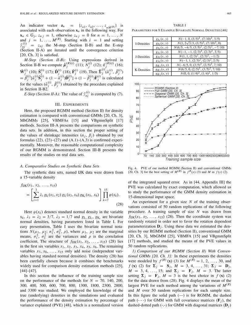
Fig. 4. PVE of our method RGMM (Section II) and conventional GMMs[20, Ch. 3] for the best setting of M(R) in f R(x) (3) and M in f (x) (2).

of the integrated squared error. As in [44, Appendix III] thePVE was calculated by exact computation, which allowed usto study the performance of the GMM density estimation in15-dimensional input space.

An experiment for a given size N of the training obser-vations consisted of 50 random replications of the followingprocedure. A training sample of size N was drawn fromfIJK(x1, x2, . . . , x15) (28). Then the coordinate system wasrandomly rotated in order not to favor the rotation dependentparameterization D j . Using these data we estimated the den-sities by our RGMM method (Section II), conventional GMM[20, Ch. 3], MbGMM [25], VBMFA [15] and VBgmmSplit[17] methods, and studied the means of the PVE values in50 random replications.

1) Comparison of our RGMM (Section II) With Conven-tional GMMs [20, Ch. 3]: In these experiments the densitieswere modeled by f (R) (x) (3) for M(R) = 1, 2, . . . , 30, andf (x) (2) for � j = S j , M = 3, 4, . . . , 31; � j = D j ,M = 3, 4, . . . , 15; and � j = F j , M = 3. The lattersetting � j = F j , M = 3 is the best choice in f (x) (2)for the data drawn from (28). Fig. 4 displays the mean of thelargest PVE for each method among the variations of M(R)

and M over 50 random replications for each sample size.In this figure the solid path (—) is for RGMM, the dashedpath (- - -) for GMM with full covariance matrices (F j ), thedashed-dotted path (-.-) for GMM with diagonal matrices (D j )


Fig. 5. PVE of our RGMM (employing NEC), MbGMM [25] (employingBIC), and VBMFA [15] and VBSplitGMM [17] methods (employing VBmodel selection).

and the dotted path (· · · ) for GMM with spherical covariancematrices (S j ). The bars represent the standard error of thePVE values. Observing Fig. 4 it can be concluded that RGMM(—) achieves the largest PVE for N < 1300. This resultis not surprising, because the goal of the regularization isto overcome overfitting, which is pronounced as the trainingsample size decreases. For N > 1300, RGMM converges tothe GMM with full covariance matrices. The latter is quiteobvious result because of the exact modeling of the underlyingdensity fIJK(x1, x2, . . . , x15) (28) by the GMM with fullcovariance matrices.

2) Comparison of our RGMM Method (Section II) WithMbGMM [25], VBMFA [15], and VBgmmSplit [17]: In theprevious section, RGMM was compared with conventionalGMMs for the best setting of the number of componentsM(R) in f (R) (x) (3) and M in f (x) (2) according to thelargest PVE (which employs the knowledge of the underlyingdensity fIJK(x1, x2, . . . , x15) (28)). In this comparative studyM and the parameterizations of � j in f (x) (2) and M(R)

in f (R) (x) (3) are set by model selection procedures, whichuse the training data only. MbGMM [25] selects parameters inf (x) (2) by Bayesian information criterion (BIC) [6], whileVBMFA [15] and VBgmmSplit [17] by variational Bayes (VB)computations. Our selection of M(R) in f (R) (x) (3) cannot beconsistent with the model selection of MbGMM [25], becauseof the lack of the explicit expression for the number of the freeparameters in � j (α j , β j ) (4), which is needed in BIC. In thispaper a suitable M(R) was set by normalized entropy criterion2

(NEC) [7], [8], [49], which does not require calculation of thenumber of free parameters in � j (α j , β j ) (4).

Fig. 5. shows the mean values of PVE for the comparedmethods over 50 randomly drawn training sets fromfIJK(x1, x2, . . . , x15) (28). Observing the paths in Fig. 5 itcan be concluded that our RGMM method (solid path “—”)gains the largest PVE for small sizes of the training sets

2NEC was proved [8] to be suitable in selection of M in f (x) (2) and nota good choice for setting both M and the parameterization of � j in f (x) (2).In the latter case BIC is better choice, which is used in MbGMM [25].

Fig. 6. PVE of RGMM (Section II) and MbGMM [25] employing NEC andMCCV, and BIC and MCCV respectively.

(N < 700).In order to justify the employment of NEC in RGMM

(Section II), a Monte Carlo cross validation (MCCV) [10]model selection was carried out for our method, and in addi-tion for comparison, we applied MCCV for MbGMM [25].MCCV is a computationally demanding procedure, which wasproved [10] to be highly accurate for GMM model selection.As in [10] we ran MCCV using a half of the training pointsfor validation in 30 Monte Carlo replications. Fig. 6 showsthe obtained PVE values of our RGMM (dashed path “- - -”) and MbGMM [25] (dotted path “· · · ”). The PVE valuesof the methods employing NEC and BIC (which appearin the previous Fig. 5) are presented in Fig. 6 again forconvenient comparison. The behavior of the paths in Fig. 6shows that RGMM performs for both MCCV (- - -) and NEC(—) model selection procedures similarly, while PVE valuesof MbGMM have been enlarged by MCCV (· · · ) compared toBIC model selection (-.-). The latter result is consistent withthe observation in [10].

Fig. 7 presents the averaged negative validated log-likelihood for different validation sample sizes (1/2N =35, 70, . . . , 1650) versus various M(R) in f (R) (x) (3) over 50randomly drawn training sets from fIJK(x1, x2, . . . , x15) (28)and 30 validation Monte Carlo replications. For conveniencethe log-likelihood is normalized3 by dividing to the validationsample size. In these runs MCCV selected (according to M(R)

implying a minimum of the negative validated log-likelihood)M(R) = 2 for 35, 70 and 100 validation points, and M(R) = 3for the validation sample sizes larger than 100. The valueM(R) = 3 is the actual number of the Gaussian componentsin the underlying density fIJK(x1, x2, . . . , x15) (28), whichconfirms the proper model selection by MCCV.

Table II presents the averaged values of the selected M(R)

by NEC in RGMM (Section II) for various training samplesizes. According to the obtained results NEC tends to selectM(R) = 3, which indicates that NEC could be a good choice

3In [10] normalized negative validated log-likelihood is named negativevalidated log-likelihood per point.


Fig. 7. Normalized negative validated log-likelihood of RGMM (Section II)for various M(R) and validation sample sizes.

TABLE II

AVERAGED VALUE OF M(R) FOR NEC MODEL SELECTION IN

RGMM (SECTION II) OVER 50 RANDOM REPLICATIONS FOR

VARIOUS TRAINING SAMPLE SIZES

Training SampleSize4

Mean Value ofM(R)

Standard Error ofthe Mean

70 2.56 0.12

200 2.50 0.11

400 2.63 0.09

800 2.80 0.07

1800 2.83 0.06

3300 2.83 0.06

for model selection in our method.3) Study the Values of Shrinkage Intensities (α j , β j ),

j = 1, 2, 3 in f (R) (x) (3) for M(R) = 3: Here RGMM wasran for M(R) = 3 on 50 random training sets of various sizes(N = 70, 140, . . . , 3300) from density fIJK(x1, x2, . . . , x15)(28) and the averaged values of the shrinkage intensities(α j , β j ), j = 1, 2, 3 were computed. Fig. 8 displays thepaths of the values of the weights α jβ j ,

(1 − α j

)β j , 1 − β j ,

which give the contribution of spherical (S j ), diagonal (D j )and full (F j ) covariance matrices in � j (α j , β j ) (4). In Fig. 8,a gradual increase in the weights 1 − β j of F j and a decreaseof the weights α jβ j and

(1 − α j

)β j of S j and D j for larger

sample sizes could be observed. The latter reflects the desiredcontribution of F j , S j and D j in RGMM. The behavior of thepaths for the weights α j β j ,

(1 − α j

)β j and 1 − β j confirms

that the formulas derived in Section II-B2 compute the propervalues of α j , β j for adjusting the complexity of � j (α j , β j )(4) to the size of the training sample. The latter justifies theenlargement of the PVE by our RGMM method with respectto the PVE of the conventional GMM (reported in Fig. 4).

4In Table II we report the results for some of the training sample sizes. Forthe other sizes 140, 300, 500-700, 1300, 2300 and 2800 the obtained meanvalues of M(R) are in the same range 2.56-2.83 as the M(R) values in thetable.

Fig. 8. Weights α j β j ,(1 − α j

)β j , 1 − β j giving the contribution of S j ,

D j and F j in � j (α j , β j ) (4) for j = 1, 2, 3.

4) Computational Complexity of the M-Step (Section II-B)of our EM Algorithm: In addition to the calculationsin the conventional M-step ((10)–(12) and (16)–(17))we compute the optimal shrinkage intensities (α

(i)j , β

(i)j )

by (22), (23)–(27), and (A.1)–(A.3). To evaluate the com-plexity of the latter calculations, the averaged number ofkFlops and seconds5 needed in our M-step for M(R) = 3in estimating the densities with different dimensionality werecomputed. In this experiment, data sets of size N =70, 140, . . . , 3300 were drawn from the 15-dimensionaldensity fIJK(x1, x2, . . . , x15) (28), and from the densities ofsmaller dimensionality:

fI (x1, x2) =3∑

i=1

λi gIi (x1, x2) (29)

fIJ (x1, x2, x3, x4) =3∑

i=1

λi gIi (x1, x2)gJi (x3, x4) (30)

fIJK (x1, x2, . . . , x6) =3∑

i=1

λi gIi (x1, x2)gJi (x3, x4)gKi (x5, x6)

(31)

for gIi , gJi , gKi the bivariate normal densities, having parame-ters listed in Table I. The obtained results, presented in Fig. 9,indicate an increase of the complexity for larger dimension ofthe observations and larger size of training samples.

In addition, the run time of our RGMM method wasmeasured for M(R) = 1, 2, . . . , 30 in f (R) (x) (3). Then itwas compared to the total run time of conventional GMMsf (x) (2) for � j = F j , M = 1, . . . , 6; � j = D j ,M = 3, . . . , 15 and � j = S j , M = 3, . . . , 31 on 50 randomtraining sets drawn from fIJK(x1, x2, . . . , x15) (28) of sizeN = 70, 140, 200, 300, 400, 500, 600, 700, 800, 1300, 1800,2300, 2800, and 3300. In both cases approximately the same

5The time of running was measured on processor Intel Core 2 Duo E8400@3600 MHz with RAM 4 GB DDR3 1333 MHz.


Fig. 9. Averaged number of kFlops and seconds of the M-step (Section II-B)for densities with various dimensionalities and various sizes of the trainingsamples.

run time of 3.5 hours was obtained, which indicates a reason-able computational complexity of our RGMM (Section II).

B. Comparative Studies on Clustering of Real Data Sets

GMMs are widely applied due to their interpretation byviewing each fitted Gaussian component as a distinct clusterin the data. Here we study the clustering ability of RGMM(Section II) and MbGMM [25] on the image segmentationdata sets from UCI machine learning repository [50]. Thesesets comprise 330 instances from several types of images. Twoclustering scenarios were examined: 1) clustering of imageshaving similar textures—brickface, foliage, and window; and2) clustering of images with significantly different textures—sky, cement and grass. For each scenario we drew randomlyn = 250 instances per image type and ran principal componentanalysis reduction [43] of the dimension to 6, retaining 99% ofthe variances of the original features. After this we computedf (R) (x) (3) by RGMM (Section II), employing NEC forsetting M(R), and f (x) (2) by MbGMM [25] using BIC forchoosing M and the parameterizations of � j . Then the trainingdata were splitted to clusters by assigning an instance to thej th cluster according the maximum probability of responsibil-ity [1, Ch. 9.2] of the j th component of the GMMs for theinstance. We denote by n j the resulted number of the instancesin the cluster j = 1, . . . , M, where M = M for f (x) (2) andM = M(R) for f (R) (x) (3). Finally the clustering performanceof the methods have been evaluated by F-measure [51]

F = 1

3

3∑

i=1

maxj

{2

(ni j

/n) (

ni j/

n j)

(ni j

/n j

) + (ni j

/n)}

(32)

where the sum in the right hand side of (32) is over thenumber of types of images, which is 3 in our experiment;ni j , i = 1, 2, 3, j = 1, 2, . . . , M is the number of instancesfrom the image type i which have been assigned to cluster j ;and as was defined previously, n = 250 denotes the number ofinstances per image type and n j -the number of the instancesin the cluster j . Table III presents the averaged F-measure,and the averaged number of the clusters (M in f (x) (2) andM(R) in f (R) (x) (3)) over 50 random drawings of n = 250

TABLE III

AVERAGED F-MEASURE (32) AND THE AVERAGED NUMBER OF THE

CLUSTERS FOR TWO CLUSTERING SCENARIOS: 1) BRICKFACE, FOLIAGE

AND WINDOW WITH SIMILAR TEXTURES, AND 2) SKY, CEMENT AND

GRASS HAVING SIGNIFICANTLY DIFFERENT TEXTURES

Clusteringscenario

Method F-measure Number ofthe clusters

1

MbGMM [25] 0.4257 6.2333

employing BIC (0.0057)* (0.2245)

RGMM (Section II) 0.4919 2.0333

employing NEC (0.0012) (0.0328)

2

MbGMM [25] 0.8227 6.8000

employing BIC (0.0145) (0.3477)

RGMM (Section II) 0.9505 3.5333

employing NEC (0.0152) (0.1129)

*In the parenthesis we give the standard errors of the means

instances per image type. The significance of the differencesof the averaged F-measures between RGMM (Section II) andMbGMM [25] was computed by a paired t-test [52]. It wasfound that for both scenarios the enlargement of the F-measurein our RGMM method is significant (with level of significanceSig.<0.01). Looking at the number of the clusters obtained bythe methods (last column of Table III), we observe a largernumber than 3 for MbGMM [25] and a smaller number than3 for RGMM, where 3 is the actual number of types of theimages. The latter observations are consistent with previousstudies for BIC and NEC model selection procedures [9].Summarizing the results from Table III, we conclude that ourRGMM (Section II) can be an attractive choice in solvingcluster analysis problems.

IV. CONCLUSION

This paper proposed a method for multivariate probabilitydensity function estimation by means of a RGMM, whichshrinks the maximum likelihood estimator of the componentcovariance matrices to suitable chosen restricted targets. InSection II, we derived an EM algorithm, which enables usto calculate specific shrinkage intensities for the covariancematrices in our RGMM, which was not previously possible[27]–[29]. Section III presents a comparison of the pro-posed method with recent model-based and VB approximationmethods on synthetic and real data sets. The results showthat our method achieved a significant improvement in theperformance of multivariate probability density estimation bya reasonable enlargement of the computation complexity ofthe conventional Gaussian mixture density estimation.

In Section II-B2 the analytical shrinkage theory of LW [23],[30] was employed in the derivation of explicit formulas forcomputing the values of shrinkage intensities in our specificcovariance matrix model (see (4)), which comprises two targetmatrices. To the best of our knowledge, these formulas do notappear in the literature and are derived for the first time inthis paper.

It must be noted that analytical shrinkage estimation of thecovariance matrix, which is stimulated by LW theory [23],[30] is an area of active research. Recently, oracle approxi-


mating shrinkage [31], shrinkage-to-tapering oracle [32], andimproved Stein-type shrinkage [33] have been proposed forestimation covariance matrix when the training observationswere Gaussian distributed and the shrinkage model was lin-ear and comprised one target only. In the case of ellipti-cally distributed training observations, regularized and robustcovariance matrix estimation was derived in [34] and [35].Recently, in [36] and [37], a nonlinear shrinkage estimator ofthe covariance matrix was proposed, which gives significantlyimproved results compared to the linear shrinkage estimator[23], [30]. In future research, we intend to employ someof these recent developments for regularization of Gaussianmixture density estimation.

APPENDIX

SAMPLE COUNTERPARTS

Here, following [23], we derive the sample counterparts,denoted by E{·}, var{·} and cov{·, ·}, of the populations oper-ations E{·}, var{·}and cov{·, ·} in (23)–(27). First, we computeE{F(i)

j } = F(i)j , E{D(i)

j } = D(i)j and E{S(i)

j } = S(i)j , for F(i)

j

(19), D(i)j (18), and S(i)

j (17). Then we denote (l, m)-entries

of the matrices F(i)j , D(i)

j , and S(i)j by f ( j )

lm , d( j )lm , and s( j )

lm forl, m = 1, 2, . . . , P , and l- or m-entry of a training point xn byxnl and xnm . After this assuming that xn are independent andidentically distributed (i.i.d) entails that the entries w

( j )nlm =

γnj (xnl −μ( j )l )(xnm −μ

( j )m ) of the right-hand terms of (10) are

i.i.d as well. From this we compute

var{ f ( j )lm }=var

{1

N j

N∑

n=1

w( j )nlm

}= 1

N2j

var

{N∑

n=1

w( j )nlm

}

= 1

N jvar

{f ( j )lm

}≈ 1

N j2

N∑

n=1

(w

( j )nlm − w

( j )lm

)2

(A.1)

var{s( j )ll }

= 1

N j2

N∑

n=1

(1

P

P∑

k=1

(w( j )nkk −w

( j )kk )

1

P

P∑

m=1

(w( j )nmm −w

( j )mm)

)

(A.2)

while s( j )lm = 0 for l �= m and

cov{

s( j )ll , f ( j )

ll

}= cov

{s( j )ll , d( j )

ll

}

≈ 1

N j2

N∑

n=1

(w( j )nll − w

( j )ll )

(1

P

P∑

r=1

(w( j )nrr − w

( j )rr )

)(A.3)

while cov{s( j )lm , f ( j )

lm } = cov{s( j )lm , d( j )

lm } = 0 for l �= m.In (A.1)–(A.3) w denotes sample mean.

In (A.1) the relation var{∑Nn=1 w

( j )nlm } = N j var{ f ( j )

lm }was used. The values of var{d( j )

lm }, l, m = 1, 2, . . . , P ,are obtained by taking the diagonal entries of var{ f ( j )

lm }(A.1) and setting the other entries equal to zero and finallycov{d( j )

lm , f ( j )lm } = var{d( j )

lm }.

ACKNOWLEDGMENT

The authors would like to thank the Editor-in-ChiefProf. D. Liu, the associate editor, and the reviewers for theircritical reading of the manuscript and helpful comments.

REFERENCES

[1] C. M. Bishop, Pattern Recognition and Machine Learning. New York:Springer-Verlag, 2006.

[2] G. J. McLachlan and D. Peel, Finite Mixture Models. New York: Wiley,2000.

[3] D. M. Titterington, A. F. M. Smith, and U. E. Makov, Statistical Analysisof Finite Mixture Distributions. New York: Wiley, 1985.

[4] T. Hastie, R. Tibshirani, and J. Friedman, The Elements of StatisticalLearning; Data Mining, Inference, and Prediction. Berlin, Germany:Springer-Verlag, 2001.

[5] H. Akaike, “A new look at the statistical model identification,” IEEETrans. Autom. Control, vol. 19, no. 6, pp. 716–723, Dec. 1974.

[6] G. Schwarz, “Estimating the dimension of a model,” Ann. Stat., vol. 6,no. 2, pp. 461–464, 1978.

[7] G. Celeux and G. Soromenho, “An entropy criterion for assessing thenumber of clusters in a mixture model,” J. Classificat., vol. 13, no. 2,pp. 195–212, 1996.

[8] C. Biernacki, G. Celeux, and G. Govaert, “An improvement of theNEC criterion for assessing the number of clusters in a mixture model,”Pattern Recognit. Lett., vol. 20, no. 3, pp. 267–272, 1999.

[9] C. Biernacki, G. Celeux, and G. Govaert, “Assessing a mixture modelfor clustering with the integrated completed likelihood,” IEEE Trans.Pattern Anal. Mach. Intell., vol. 22, no. 7, pp. 719–725, Jul. 2000.

[10] P. Smyth, “Model selection for probabilistic clustering using cross-validated likelihood,” Stat. Comput., vol. 10, no. 1, pp. 63–72, 2000.

[11] R. A. Baxter and J. J. Oliver, “Finding overlapping components withMML,” Stat. Comput., vol. 10, no. 1, pp. 5–16, 2000.

[12] D. J. Spiegelhalter, N. G. Best, B. P. Carlin, and A. Van Der Linde,“Bayesian measures of model complexity and fit,” J. Royal Stat. Soc.,Ser. B, Stat. Methodol., vol. 64, no. 4, pp. 583–639, 2002.

[13] G. Celeux, F. Forbes, C. Robert, and D. Titterington, “Deviance infor-mation criteria for missing data models,” Bayesian Anal., vol. 1, no. 4,pp. 651-674, 2006.

[14] S. E. Yuksel, J. N. Wilson, and P. D. Gader, “Twenty years of mixtureof experts,” IEEE Trans. Neural Netw. Learn. Syst., vol. 23, no. 8,pp. 1177–1193, Aug. 2012.

[15] Z. Ghahramani and M. J. Beal, “Variational inference for Bayesian mix-tures of factor analysers,” in Advances in Neural Information ProcessingSystems, vol. 12. Cambridge, MA: MIT Press, 2000, pp. 449–455.

[16] W. Fan, N. Bouguila, and D. Ziou, “Variational learning for finiteDirichlet mixture models and applications,” IEEE Trans. Neural Netw.Learn. Syst., vol. 23, no. 5, pp. 762–774, May 2012.

[17] C. Constantinopoulos and A. Likas, “Unsupervised learning of Gaussianmixtures based on variational component splitting,” IEEE Trans. NeuralNetw., vol. 18, no. 3, pp. 745–755, May 2007.

[18] A. Penalver and F. Escolano, “Entropy-based incremental variationalBayes learning of Gaussian mixtures,” IEEE Trans. Neural Netw. Learn.Syst., vol. 23, no. 3, pp. 534–540, Mar. 2012.

[19] C. A. McGrory and D. M. Titterington, “Variational approximations inBayesian model selection for finite mixture distributions,” Comput. Stat.Data Anal., vol. 51, no. 11, pp. 5352–5367, 2007.

[20] G. J. McLachlan and T. Krishnan, The EM Algorithm and Extensions.New York: Wiley, 2008.

[21] A. P. Dempster, N. M. Laird, and D. B. Rubin, “Maximum likelihoodfrom incomplete data via the EM algorithm,” J. Royal Stat. Soc. Ser. B,Methodol., vol. 39, no. 1, pp. 1–38, 1977.

[22] M. J. Daniels and R. E. Kass, “Shrinkage estimators for covariancematrices,” Biometrics, vol. 57, no. 4, pp. 1173–1184, 2001.

[23] O. Ledoit and M. Wolf, “A well-conditioned estimator for large-dimensional covariance matrices,” J. Multivar. Anal., vol. 88, no. 2,pp. 365–411, 2004.

[24] D. Ormoneit and V. Tresp, “Averaging, maximum penalized likeli-hood and Bayesian estimation for improving Gaussian mixture prob-ability density estimates,” IEEE Trans. Neural Netw., vol. 9, no. 4,pp. 639–650, Jul. 1998.

[25] C. Fraley and A. E. Raftery, “Model-based clustering, discriminantanalysis, and density estimation,” J. Amer. Stat. Assoc., vol. 97, no. 458,pp. 611–631, 2002.


[26] C. Fraley and A. E. Raftery, “Bayesian regularization for normal mixtureestimation and model-based clustering,” J. Classificat., vol. 24, no. 2,pp. 155–181, 2007.

[27] Z. Halbe and M. Aladjem, “Regularized mixture discriminant analysis,”Pattern Recognit. Lett., vol. 28, no. 15, pp. 2104–2115, 2007.

[28] B. C. Kuo and D. A. Landgrebe, “A robust classification procedure basedon mixture classifiers and nonparametric weighted feature extraction,”IEEE Trans. Geosci. Remote Sens., vol. 40, no. 11, pp. 2486–2494,Nov. 2002.

[29] M. M. Dundar and D. Landgrebe, “A model-based mixture-supervisedclassification approach in hyperspectral data analysis,” IEEE Trans.Geosci. Remote Sens., vol. 40, no. 12, pp. 2692–2699, Dec. 2002.

[30] O. Ledoit and M. Wolf, “Improved estimation of the covariance matrixof stock returns with an application to portfolio selection,” J. EmpiricalFinan., vol. 10, no. 5, pp. 603–621, 2003.

[31] Y. Chen, A. Wiesel, Y. C. Eldar, and A. O. Hero, “Shrinkage algorithmsfor MMSE covariance estimation,” IEEE Trans. Signal Process., vol. 58,no. 10, pp. 5016–5029, Oct. 2010.

[32] X. Chen, Z. J. Wang, and M. J. McKeown, “Shrinkage-to-taperingestimation of large covariance matrices,” IEEE Trans. Signal Process.,vol. 60, no. 11, pp. 5640–5656, Nov. 2012.

[33] T. J. Fisher and X. Sun, “Improved stein-type shrinkage estimators forthe high-dimensional multivariate normal covariance matrix,” Comput.Stat. Data Anal., vol. 55, no. 5, pp. 1909–1918, 2011.

[34] Y. Chen, A. Wiesel, and A. O. Hero, “Robust shrinkage estimation ofhigh-dimensional covariance matrices,” IEEE Trans. Signal Process.,vol. 59, no. 9, pp. 4097–4107, Sep. 2011.

[35] A. Wiesel, “Unified framework to regularized covariance estimation inscaled Gaussian models,” IEEE Trans. Signal Process., vol. 60, no. 1,pp. 29–38, Jan. 2012.

[36] O. Ledoit and S. Péché, “Eigenvectors of some large sample covariancematrix ensembles,” Probab. Theory Rel. Fields, vol. 151, nos. 1–2,pp. 233–264, 2011.

[37] O. Ledoit and M. Wolf, “Nonlinear shrinkage estimation of large-dimensional covariance matrices,” Ann. Stat., vol. 40, no. 2,pp. 1024–1060, 2012.

[38] J. H. Friedman, “Regularized discriminant analysis,” J. Amer. Stat.Assoc., vol. 84, no. 405, pp. 165–175, 1989.

[39] D. R. Hunter and K. Lange, “A tutorial on MM algorithms,” Amer. Stat.,vol. 58, no. 1, pp. 30–37, 2004.

[40] P. L. Leung and R. J. Muirhead, “Estimation of parameter matrices andeigenvalues in MANOVA and canonical correlation analysis,” Ann. Stat.,vol. 15, no. 4, pp. 1651–1666, 1987.

[41] D. G. Luenberger, Linear and Nonlinear Programming. New York:Springer-Verlag, 2003.

[42] J. Schäfer and K. Strimmer, “A shrinkage approach to large-scalecovariance matrix estimation and implications for functional genomics,”Stat. Appl. Genet. Molecular Biol., vol. 4, no. 1, p. 32, Nov. 2005.

[43] R. O. Duda, P. E. Hart, and D. G. Stork, Pattern Classification, 2nd ed.New York: Wiley, 2001.

[44] M. Aladjem, “Projection pursuit mixture density estimation,” IEEETrans. Signal Process., vol. 53, no. 11, pp. 4376–4383, Nov. 2005.

[45] K. Roeder and L. Wasserman, “Practical Bayesian density estimationusing mixtures of normals,” J. Amer. Stat. Assoc., vol. 92, no. 439,pp. 894–902, 1997.

[46] M. Wand and M. Jones, “Comparison of smoothing parameterizationsin bivariate kernel density estimation,” J. Amer. Stat. Assoc., vol. 88,no. 422, pp. 520–528, 1993.

[47] M. P. Wand and M. C. Jones, Kernel Smoothing. New York: Chapman &Hall, 1995.

[48] J. H. Friedman, W. Stuetzle, and A. Schroeder, “Projection pursuitdensity estimation,” J. Amer. Stat. Assoc., vol. 79, no. 387, pp. 599–608,1984.

[49] C. Biernacki, G. Celeux, G. Govaert, and F. Langrognet, “Model-basedcluster and discriminant analysis with the MIXMOD software,” Comput.Stat. Data Anal., vol. 51, no. 2, pp. 587–600, 2006.

[50] A. Frank and A. Asuncion. (2010). UCI Machine Learning Reposi-tory. School Information & Computer Science, Univ. California, Irvine[Online]. Available: http://archive.ics.uci.edu/ml/

[51] C. J. Rijsbergen, Information Retrieval. London, U.K.: Butterworth,1979.

[52] R. G. D. Steel and J. H. Torrie, Principles and Procedures of Statistics:A Biometrical Approach. New York: McGraw-Hill, 1980.

Zohar Halbe received the B.Sc., M.Sc. and Ph.D.degrees in electrical and computer engineering fromthe Ben-Gurion University of the Negev, Beer-Sheva, Israel, in 2001, 2004, and 2009, respectively.His doctoral dissertation focused on mixture modelsfor density estimation.

He was a Lecturer with the Ben-Gurion Universityof the Negev from 2009 to 2012. He is currently aResearch Fellow with the Human Cognitive Neuro-science Laboratory, Faculty of Psychology, Depart-ment of Psychology, Hebrew University, Jerusalem,

Israel, and the Head of the Algorithm Department, ElMindA Ltd. His currentresearch interests include biomedical signal processing, statistical patternrecognition, neural networks for pattern recognition, multivariate densityestimation, and blind source separation.

Maria Bortman received the B.A. degree in elec-trical engineering from Moscow Railway TransportUniversity, Moscow, Russia, in 1999, and the M.Sc.degree in electrical and computer engineering fromthe Ben-Gurion University of the Negev, Beer-Sheva, Israel, in 2006, where she is currently pursu-ing the Ph.D. degree.

Her current research interests include statisti-cal pattern recognition, neural networks for pat-tern recognition, multivariate density estimation, andindependent component analysis.

Mayer Aladjem (M’98) received the M.Sc. degreein electrical engineering and applied mathematicsand the Ph.D. degree in electrical engineering fromthe Technical University of Sofia, Sofia, Bulgaria.

He was a Professor of biomedical cybernetics withthe Bulgarian Academy of Sciences. He joined theDepartment of Electrical and Computer Engineering,Ben-Gurion University of the Negev, Beer-Sheva,Israel, in 1990, where he is a Professor and theHead of Pattern Recognition and Intelligent DataAnalysis Laboratory. His current research interests

include statistical pattern recognition, neural networks for pattern recognition,multivariate density estimation, blind source separation, independent compo-nent analysis, feature extraction, reduction, and analysis, and applications insignal and image processing.

Prof. Aladjem was the Chairman of the 2001 International Symposium onAdvances in Intelligent Data Analysis, Bangor, Wales, U.K., and was theGuest Editor of the Special Edition: Advanced Data Analysis and BiomedicalApplications in the journal Knowledge-Based Intelligent Engineering Sys-tems. He was a keynote lecturer in the international conferences, includingCIMA’2001, University of Wales, Bangor, U.K., ICAMEE 2005, Sozopol,Bulgaria, and IC3K 2011, Paris, France. He is currently an Associate Editorof the journal Pattern Analysis & Applications. For more information, seehttp://www.ee.bgu.ac.il/∼aladjem/.

Documents

Regularized Mixture Density Estimation With an Analytical Setting of Shrinkage Intensities