Embed Size (px)
Citation preview

ESAIM: PROCEEDINGS AND SURVEYS, Vol. ?, 2017, 1-10Editors: Will be set by the publisher
REGRESSION MONTE CARLO FOR MICROGRID MANAGEMENT
CLEMENCE ALASSEUR 1, ALESSANDRO BALATA 2, SAHAR BEN AZIZA 3, ADITYAMAHESHWARI 4, PETER TANKOV 5 AND XAVIER WARIN 6
Abstract. We study an islanded microgrid system designed to supply a small village with thepower produced by photovoltaic panels, wind turbines and a diesel generator. A battery storagesystem device is used to shift power from times of high renewable production to times of highdemand. We build on the mathematical model introduced in [12] and optimize the diesel con-sumption under a “no-blackout” constraint. We introduce a methodology to solve microgrid man-agement problem using different variants of Regression Monte Carlo algorithms and use numericalsimulations to infer results about the optimal design of the grid.
1. INTRODUCTION
A Microgrid is a network of loads and energy generating units that often include renewable sourceslike photovoltaic (PV) panels and wind turbines alongside more traditional forms of thermal electricityproduction. These microgrids can be part of the main grid or isolated. Communities in rural areas of theworld have long now enjoyed the installation of isolated microgrid systems that provide a reliable and oftenenvironment-friendly source of electricity to meet their power needs.
The elementary purpose of a microgrid is to provide a continuous electricity supply from the variablepower produced by renewable generators while minimizing the installation and running costs. In this kindof systems, the uncertainty of both, the load and the renewable production is high and its negative effect onthe system stability can be mitigated by including a battery energy storage system in the microgrid. Energystorage devices ensure power quality, including frequency and voltage regulation (see [10]) and providebackup power in case of any contingency. A dispatchable unit in the form of diesel generator is also usedas a backup solution and to provide baseload power.
In this paper, we consider a traditional microgrid serving a small group of customers in islanded mode,meaning that the network is not connected to the main national grid. The system consists of an intermittentrenewable generator unit, a conventional dispatchable generator, and a battery storage system. Both theload and the intermittent renewable production are stochastic, and we use a stochastic differential equation(SDE) to model directly the residual demand, that is, the difference between the load and the renewableproduction. We then set up a stochastic optimization problem, whose goal is to minimize the cost of usingthe diesel generator plus the cost of curtailing renewable energy in case of excess production, subject tothe constraint of ensuring reliable energy supply. A regression Monte Carlo method from the mathematicalfinance literature is used to solve this stochastic optimization problem numerically. Three variants of theregression alrogithm, called grid discretization, Regress now and Regress later are proposed and compared
1 EDF R&D - FIME, Palaiseau, France; e-mail: [email protected] University of Leeds, Woodhouse Lane, Leeds LS2 9JT, United Kingdom; e-mail: [email protected] University of Tunis El Manar,ENIT-LAMSIN, BP.37, Le Belvédère 1002 Tunis, Tunisia; e-mail: [email protected] University of California, Santa Barbara, USA; e-mail: [email protected] CREST-ENSAE, Palaiseau, France; e-mail: [email protected] EDF R&D - FIME, Palaiseau, France; e-mail: [email protected]
c© EDP Sciences, SMAI 2017

in this paper. The numerical examples illustrate the performance of the optimal policies, provide insightson the optimal sizing of the battery, and compare the policies obtained by stochastic optimization to theindustry standard, which uses deterministic policies.
The optimization problem arising from the search for a cost-effective control strategy has been exten-sively studied. Three recent survey papers [13,17,18] summarize different methods used for optimal usage,expansion and voltage control for the microgrids. Heymann et. al. [11,12] transform the optimization prob-lem associated with the microgrid management into an optimal control framework and solve it using thecorresponding Hamilton Jacobi Bellman equation. Besides proposing an optimal strategy, the authors alsocompare the solution of the deterministic and stochastic representation of the problem. However, similarlyto most PDE methods, this approach suffers from the curse of dimensionality and as a result, it is difficultto scale. The main contribution of this paper is to solve the microgrid control problem using RegressionMonte Carlo algorithms. In contrast to existing approaches, the method used in this paper is more easilyscalable and works well in moderately large dimensions [3].
Identifying the optimal mix, the size and the placement of different components in the microgrid isan important challenge to its large scale use. The papers [14, 15] use mixed-integer linear programmingto address the design problem and test their model on a real data set from a microgrid in Alaska. In asimilar work, [16] studied the economically optimal mix of PV, wind, batteries and diesel for rural areas inNigeria. In [9], optimal battery storage sizing is deduced from the autocorrelation structure of renewableproduction forecast errors. In this paper, we propose an alternative approach for the optimal sizing of thebattery energy storage system, assuming stochastic load dynamics and fixed lifetime of the battery. Ourin-depth analysis of the system behavior leads to practical guidelines for the design and control of islandedmicrogrids.
Finally, several authors [5–7] used stochastic control techniques to determine optimal operation strate-gies for wind production – storage systems with access to energy markets. In contract to these papers, inthe present study, energy prices appear only as constant penalty factors in the cost functional, and the mainfocus is on the stable operation of the microgrid without blackouts.
The rest of the paper is organized as follows: In section 2 we describe the microgrid model and introducethe different components of the system, in section 3 we translate the problem of managing the microgrid ina stochastic optimization problem and present the dynamic programming equation that we intend to solvenumerically. Section 4 introduces the numerical algorithms used to solve the control problem, we give ageneral framework for solving the dynamic programming equation and we then provide three algorithmsfor the approximation of conditional expectations. In section 5 we illustrate the results of the numericalexperiments, identify the best algorithm among those we studied and then employ it to analyze the systembehavior. We conclude with section 6 where the estimated policy for the stochastic problem is compared,in an appropriate manner, with a deterministically trained one; the aim is to provide evidence that industry-widespread deterministic approaches underperform stochastic methods.
2. MODEL DESCRIPTION
In this section, we will discuss the topology of the microgrid, its operation, components and their re-spective dynamics. Although we discuss a simplified microgrid model, more complicated typologies canbe studied using straightforward generalizations of the methods presented in this paper.
Consider a microgrid serving a small, isolated village; most of the power to the village is supplied bygenerating units whose output has zero marginal cost, is intermittent and uncontrolled. Additional power issupplied by a controlled generator whose operations come alongside a cost for the microgrid owner (eitherthe community itself or a power utility). Often the intermittent units include PV panels and wind turbines,while the controlled unit is often a diesel generator. In order to fully exploit the free power generated bythe renewable units at times when production exceeds the demand, microgrids are equipped with energystorage devices. These can be represented by a battery energy storage system.
The introduction of the battery in the system not only allows for inter-temporal transfer of energy fromtimes when demand is low, to times when it is higher, but also introduces an element of strategic behaviorthat can be employed by the system controller, to minimize the operational costs. Without an energystorage, diesel had to be run at all times demand exceeded production. When a battery is installed, intensity
2

and timing of output from the diesel generator can be adjusted to move the level of charge of the batterytowards the most cost effective levels.
In figure 1 we propose a schematic description of the system which might help the reader to familiarizethemselves with the microgrid, whose components are described more in depth in the following subsec-tions.
Remark 1. Note that for convenience, in the following, we will work in discrete time only. This setting isnot restrictive as in reality measurements of the systems are repeated at a given, finite, frequency. We alsoconsider a finite optimization horizon represented by the number of periods over which we want to optimizethe system operations indicated by T
FIGURE 1. The figure above shows an example of microgrid topology that contains all the ele-ments in our model. The network is arranged as follows: photovoltaic panels and wind turbinesprovide renewable generation, a diesel generator provides dispatchable power for the village and abattery storage system is used to inject or withdraw energy.
2.1. Residual Demand
Consider two stochastic processes Lt and Rt, the former represents the demand/load and the latterthe production through the renewable generators. Notice that both processes are uncontrolled and theyrepresent, respectively, the unconditional withdrawal or injection of power in the system (constant duringtime step). For the purpose of managing the microgrid, the controller is interested only in the net effect ofthe two processes denoted by the process Xt:
Xt “ Lt ´Rt ; t P t0, 1, . . . , T u. (1)
Remark 2. The state variable Xt represents the residual demand of power at each time t, such that forXt ą 0, we should provide power through the battery or diesel generator and for Xt ă 0 we can store theextra power in the battery.
For simplicity, we model the residual demand as an AR(1) process, the discrete equivalent of an Orn-stein–Uhlenbeck process. In practical applications we expect Xt to be an R-valued mean reverting processwith many different sources of noise and time dependent random parameters; our formulation avoids thecumbersome notation using constants in place of stochastic processes still providing scope for generaliza-tion. The process Xt is driven by the following difference equation, starting from an initial point X0 “ x0:
Xt`1 “ Xt ` bpΛt ´Xtq∆t` σ?
∆t ξt ; t P t0, 1, . . . , T u (2)
where ξt „ Np0, 1q, ∆t is the amount of time before new information is acquired, b is the mean reversionspeed, σ the volatility of the process and Λt is the time dependent mean reversion level.
Remark 3. In real applications the function Λt should represent the best forecast available for futureresidual demand at the time of the estimation of the policy.
3

2.2. Diesel generator
The Diesel generator represents the controlled dispatchable unit. The state of the generator is repre-sented by mt “ t0, 1u. If mt “ 0 then the diesel generator is OFF, while it is ON when mt “ 1. Whenthe engine is ON, it produces a power output denoted by dt P rdmin, dmaxs at time t, for dmin ą 0.
Notice that, in addition, when the engine is turned ON, an extra amount of fuel is burned in order for thegenerator to warm up and reach working regime. We model the cost of burning extra fuel with a switchingcost K that is paid every time the switch changes from 0 to 1. The fuel consumption of the diesel generatoris modeled by an increasing function ρpdtq which maps the power dt produced during one time step intothe quantity of diesel necessary for such output. Denoting by Pt the price of fuel at time t, the cost ofproducing dt KW of power at one time step is Ptρpdtq; for simplicity we take a constant price of the fuelPt “ p. Two examples of efficiency functions ρ are described in figure 2.
(A) ρpdq “ pd´6q3`63`d10
(B) ρpdq “ d0.9
FIGURE 2. The panels above show two examples of efficiency function (litres/KW), on the leftρpdq “ pd´6q3`63`d
10, typical of a generator designed to operate at medium regime, on the right
ρpdq “ d0.9, typical of a generator designed to operate a full capacity.
2.3. Dynamics of the Battery
The storage device is directly connected to the microgrid and therefore its output is equal to the imbal-ance between demand Xt and diesel generator output dt, when this is allowed by the physical constraint.The battery therefore is discharged in case of insufficiency of the diesel output and charged when the dieselgenerator and renewables provide a surplus of power.
Let us denote the power output of the battery by Bdt and its power rating by Bmax and Bmin, whereBmax and Bmin represent respectively the maximum and minimum output. Thus:
Bdt “Idt ´ Imax
∆t_`
Bmin _ pXt ´ dtq ^Bmax
˘
^Idt∆t
(3)
The case where Bdt ă 0, represents that the battery is charging while the case where Bdt ą 0, representsthat the battery is supplying power.
Notice then that an energy storage has a limited amount of capacity after which it can not be chargedfurther, as well as an “empty” level below which no more power can be provided from the battery. Wedenote the state of charge by the controlled process Idt which is described by the following equation:
Idt`1 “ Idt ´Bdt ∆t, t P t0, 1, . . . , T ´ 1u, Id0 “ w0 (4)
here Idt P r0, Imaxs and Bdt P rBmin, Bmaxs, for Bmin ă 0 and Bmax ą 0. For simplicity we assume that
the battery is 100% efficient. Notice that we used superscript d on Bd and Id to highlight the dependenceof these processes on the controlled diesel output dt.
Intuition tells us that the bigger the battery, the less diesel will be needed to run the operations of themicrogrid. This is true because a bigger battery would allow to store for later use a bigger proportion of
4
the excess power produced by the renewables. Batteries however are very expensive, and the cost per KWhof capacity scales almost linearly for the kind of devices we consider in this paper (parallel connection ofsmaller batteries), hence it is important to find the optimal size of battery for the needs of each specificmicrogrid.
2.4. Management of the Microgrid
The purpose of the microgrid is to provide a cheap and reliable source of power supply to at leastmatch the demand. Therefore, we search for a control policy for the diesel generator which minimizes theoperating cost and produces enough electricity to match the residual demand. In order to assess how wellwe are doing in supplying electricity, we introduce the controlled imbalance process St defined as follows:
St “ Xt ´Bdt ´ dt t P r0, T s (5)
Ideally, the owner of the Microgrid would like to have St “ 0 @ t. This situation represents the perfectbalance of demand and generation. When St ą 0 we observe a blackout, residual demand is greater thanthe production meaning that some loads are automatically disconnected from the system. The situationSt ă 0 is defined as a curtailment of renewable resources and takes place when we have a surplus ofelectricity.
We treat the two scenarios, blackout and curtailment asymmetrically. To ensure no-blackout St ď 0 andregular supply of power, we impose a constraint on the set of admissible controls:
St ď 0
i.e. dt ě Xt ´Bdt .
(6)
However, for St ă 0 i.e. surplus of electricity, we penalize the microgrid using a proportional costdenoted by C. Large penalty would lead to low level of curtailment and can be thought of as a parameterin the subsequent optimization problem.
A rigorous mathematical description of the microgrid management problem follows in section 3.
3. STOCHASTIC OPTIMIZATION PROBLEM
We state now the stochastic control problem for the diesel generator operating in a microgrid systemas described in section 2. In practice we seek a control that minimizes the cost of diesel usage pρpdq, theswitching cost K and the curtailment cost C|St|1tStă0u, under the no black-out constraint St ď 0.
Note that, given the type of control we have on the diesel generator, we can frame the optimizationproblem as a special case of stochastic control problems known as optimal switching problems.
Let us denote by Ft the filtration generated by the residual demand process pXsqts“0, the state of charge
process pIds qts“0 and the current regime mt, which represents all the information available on the system
up to time t. In practice, given the markovianity of the problem, we have that Ft is reduced to the σ-fieldgenerated by the triple pXt, I
dt ,mtq.
Let us define the pathwise value J, given by
Jpt,Xt, It,mt; dtq “T´1ÿ
s“t
1tms`1´ms“1uK` pρpdsq ` C|Ss|1tSsă0u ` gpIdT q. (7)
where pXt, It,mt; dtq “ pXs, Ids ,ms; dsq
Ts“t. As a consequence, we define the value function as:
V pt, x, w,mq “ mindt“pduqTu“t
!
E”
Jpt,Xt, Idt ,mt; dtqˇ
ˇ
ˇXt “ x, Idt “ w,mt “ m
ı)
(8)
5

subject to dt ě Xt ´Bdt @t (9a)
dt P rdmin, dmaxs Y t0u. (9b)
Bdt “Idt ´ Imax
∆t_`
Bmin _ pXt ´ dtq ^Bmax
˘
^Idt∆t
(9c)
where (9a) represents the black-out constraints translated for the power produced by the diesel generator,(9b) represents the minimum and maximum power output of the generator and (9c) models the physicalconstraints of the battery: maximum input/output power and maximum capacity.
From equation (8), we can write the associated dynamic programming formulation which helps un-derstand the structure of the problem composed of two optimal control problems: an optimal switchingproblem between being in the regime ON or OFF, and another absolutely continuous control problemassuming the regime is ON. The equation reads as follows:
V pt, x, w,mq “ mindPUt
´
1tmt`1´mt“1uK` pρpdq ` C|St|1tStă0u ` Cpt, x, w,m; dq¯
, (10)
where
Cpt, x, w,m; dq “ ErV pt` 1, Xt`1, It`1,mt`1q|Xt “ x, It “ w, dt “ d,mt “ ms,
is the conditional expectation of the future costs and Ut is the collection of admissible controls d at eachtime step t, i.e.
Ut :“ tdt : equations (9a) - (9c) are satisfied and dt adapted to Ftu. (11)
In order to ensure that the set of admissible controls is nonempty we introduce the following assumption:
Assumption 1. The diesel generator is powerful enough to supply demand at all times, i.e there is alwaysa control d that satisfies the blackout constraint.
Remark 4. We enforce assumption 1 by redefining the residual demand process with a truncated versionof (1), such that Xt “ minpXt, Xmaxq is the residual demand. In practice this is reasonable because themaximum power that could be required from the microgrid is known apriori and the diesel generator isgenerally sized to the maximum capacity installed on the system. For the sake of notational simplicity, wewill drop the „ on the variable Xt from the following sections.
Note that (10) provides a direct technique to solve problem (8), iterating backward in time from aknown terminal condition and solving a static, one period, optimization problem at each time step. Theonly difficulty in this procedure lies in the estimation of conditional expectations of future value function,which can not be computed exactly. In the next section 4 we will focus on the numerical solution of (8).
4. NUMERICAL RESOLUTION
In this section we describe the algorithm which we want to employ in the solution of the energy man-agement problem for the Microgrid system described in section 3. The main mathematical difficulty comesfrom the approximation of conditional expectations in (10), which we will tackle using a family of methodscalled Regression Monte Carlo.
The algorithm we propose fully exploits the dynamic programming formulation (10): we start gener-ating a set of simulations (scenarios) of the process X , which we will refer to as training points, then weoptimize our policy so that it performs well, on average (weighted on the probability of each scenario), onthe different scenarios.
In practice, we initialize the value function at last time step in the backward procedure to be equal tothe terminal condition g. We then iterate backward in time and at each time step over each training pointwe choose the control that minimizes the sum of one step cost function and the estimated conditionalexpectation of the future costs Cpt, x, w,m; dq. Note that, as expected, the conditional expectation is a
6

function of time, the state of the system px,wq and the state of the diesel generator, represented by theON/OFF switch m and the control d.
As the iteration reaches the initial time point we collect a set of optimal actions for each time step andmany different scenarios; in addition, since the problem is Markovian, we can summarize such strategiesin the form of control maps: best action at each time t given a pair of state variables pXt, Itq and state ofthe diesel generator mt. We propose three different techniques to compute C in section 4.1.
A fair assessment of the quality of the control policies approximated by the algorithm just introduced isobtained by running a number of forward Monte Carlo simulations of the residual demand, controlling thesystem using such policies and then taking the average performance.
We give a general description of the pseudo code in algorithm 1.
Remark 5. Notice that it is typical of Regression Monte Carlo algorithms to provide the optimal policyonly implicitly, in the form of minimizer of an explicit parameterized function. The outputs of the algorithmare therefore the parameters (regression coefficients) of such function.
4.1. Regression for continuation value
In this section we present the numerical techniques we use to estimate conditional expectations Cpt, x, w,m; dqin algorithm 1. These techniques belong to the realm of Regression Monte Carlo methods, and in partic-ular these specifications allow to deal with degenerate controlled processes (the inventory). We focus ontwo main variants: a two dimensional approximation of the conditional expectation and a discretisationtechnique which considers a collection of one dimensional approximations.
In particular, we test three algorithms: Grid Discretisation, Regress Now and Regress Later. GridDiscretization is characterized by a one dimensional projection in the residual demand dimension repeatedat different inventory points. Regress Now/Later, on the other hand, use a two dimensional regression inresidual demand and inventory. Moreover, while Grid Discretization and Regress Now require projectionof the value function at t` 1 on Ft measurable basis functions, Regress Later requires an Ft`1 projection.For details on these techniques see [1] for regress later, [2, 19] for GD and [4] for 2D regress now. Notethat in the three algorithms we repeat the regression approximation for both values of m. An open sourceplatform has also been developed to numerically solve wide variety of stochastic optimization problemsin [8].
Let us denote by tXjt uMj“1 the collection of training points at time t, similar notation is used for the
inventory tIjt uMj“1.
4.1.1. Grid Discretisation
Grid discretisation is characterized by a one dimensional approximation of the conditional expectationrepeated at different levels of inventory. Let ΥI “ tw0 “ 0, . . . , wD “ Imaxu be a discretisation of thestate space of the inventory and tXj
t uM,Nj“1,t“1 be generated from a forward simulation of the dynamics of
X . We define the approximation of the continuation value on the grid ΥI by regressing the set of valuefunctions tV pt` 1, Xj
t`1, wiquMj“1 over the basis functions tφkpxquKk“1 for each twiuDi“0, obtaining:
Cpt, x, wi;mq “Kÿ
k“1
αtk,i,mφkpxq , i “ 0, 1, . . . , D,
where we compute a collection of regression coefficients through least square minimization
αti,m “ argminaPRK
! 1
M
Mÿ
j“1
`
V pt` 1, Xjt`1, wi,mq ´
Kÿ
k“1
akφpXjt q˘2)
,
where we define RK Q αti,m “ pαt1,i,m, . . . , αtK,i,mq.Note that the least square projection is a sample estimation of the L2 projection induced by the condi-
tional expectation, for this reason we can approximate the function Cpt, ¨q using a least square projection ofthe value function at time t` 1. However, as we have not included the inventory in the basis functions, we
7

Algorithm 1 Regression Monte Carlo algorithm for Microgrid managementinput: number of basis K, number of training points M , discretisation of the inventory D, time-steps N .1: optimization:2: if Inventory discretisation then3: Generate a customary grid tw0, . . . , wDu points over the domain of It.4: Simulate tXj
t uM 1,Nj,t“1 according to its dynamics where M 1 “M{pD ` 1q;
5: Define tXjt , I
jt uMj“1 as cross product of tXj
t uM 1
j“1 and twjuDj“0 for @t
6: if Regression 2D then7: if Regress Later then8: Generate tXj
t , Ijt uM,Nj,t“1 accordingly to a distribution µ;
9: if Regress Now then10: Generate tXj
t uM,Nj,t“1 according to its dynamics and tIjt u
M,Nj,t“1 according to a distribution µ;
11: Initialize the value function V pN,XjN , I
jN , 1q “ V pN,Xj
N , IjN , 0q “ gpIjN q, @j “ 1, . . . , M ;
12: for t “ N to 1 do13: Compute the approximated continuation value C using Algorithms 3 or 214: for j “ 1 to M do15: for m “ 0 to 1 do16: F “ CpXj
t , Ijt ; 0, 0q
17:
V pt,Xjt , I
jt ,mq “
$
’
&
’
%
´
mindPUtzt0u
!
pρpdq ` C|St|1tStă0u ` CpXjt , I
jt ; 1, dq
)
`K1tm“0u
¯
^ F if 0 P Ut
mindPUt
!
pρpdq ` C|St|1tStă0u ` CpXjt , I
jt ; 1, dq
)
`K1tm“0u otherwise
18: simulation:19: initialize processes20: for t “ 1 to N ´ 1 do21: for j “ 1 to M do22: F1 “ CpXj
t , Ijt ; 0, 0q
23: F2 “ mindPUtzt0u
!
pρpdq ` C|St|1tStă0u ` CpXjt , I
jt ; 1, dq
)
`K1tmj
t“0u
24: mjt`1 “ 1tp0RUtq or p0PUt and F2ăF1qu
25: if mjt`1 “ 1 then
26: dt “ argmindPUt
!
pρpdq ` C|St|1tStă0u ` CpXjt , I
jt ; 1, dq
)
27: compute Xjt`1 and Ijt`1 “ Ijt ´B
dt ∆t
28: Jjt`1 “ Jjt ` pρpdtq ` C|St|1tStă0u `K1tmt`1´mt“1u
29: V p0, x, w,mq “ 1M
řMj“1pJ
jN ` gpI
jN qq
output: control policy tdtu, value function V .
need to interpolate between values of Cpt, x, wi;mq in order to obtain an estimation of the value functionfor It P pwi, wi`1q. Let us define by Cpt, x, w;m, dq the linear interpolation
Cpt, x, w;m, dq “ ωpt, w, dqCpt, x, wi,mq``
1´ωpt, w, dq˘
Cpt, x, wi`1,mq , w´Bdt ∆t P rwi, wi`1q,
where ωpt, w, dq “ wi`1´w`Bdt ∆t
wi`1´wiand i “ 0, . . . , D.
Details of the algorithms are given in the pseudocode 2.8

Algorithm 2 Regression technique for continuation value: Grid Discretisation
input: tV pt` 1, Xjt`1, I
jt`1,mqu
Mj“1, tφkuKk“1.
1: for i “ 0 to D do
2: αtm “ argmina
! Mř
j“1
´
V pt` 1, Xjt`1, wi,mq ´
Kř
k“1
akφkpXjt q
¯2)
;
3: Define Cpt, x, wi,mq “řKk“1 α
tk,i,mφkpxq, m “ 0, 1;
4: Define Cpt, x, w;m, dq “wi`1´w`B
dt ∆t
wi`1´wiCpt, x, wi;m, dq `
w´Bdt´wi
wi`1´wiCpt, x, wi`1;m, dq, w P
rwi, wi`1q, m “ 0, 1.
output: C, tαtk,i,muK,D,1k“1,i“1,m“0.
4.1.2. 2D Regression
Contrary to the grid discretisation approach, the 2D regression methods approximate the conditionalexpectation of the value function as a surface, function of both residual demandX and inventory I , withoutthe need for interpolation. In the problem we consider, the control only acts on a degenerate (deterministic)process and we can therefore test two specifications of the method: “Regress Now”, where we project overtφkpXt, It`1qu
Kk“1 and “Regress Later”, where we project over tφkpXt`1, It`1qu
Kk“1. The terminology
Regress Now or Regress Later is attributed to the time step of the exogenous variable Xt used in theprojection.
In Regress Now, we generate training points tXjt uM,Nj“1,t“1 from a forward simulation of the dynamics of
X and tIjt uM,Nj“1,t“1 from a distribution µN on r0, Imaxs. In Regress Later, on the other hand, we generate
both processes tXjt , I
jt uM,Nj“1,t“1 from an appropriate distribution µL, for details see [1]. In the following we
will generalize the discussion of the two approaches by using the subscript r with realization t to indicateRegress Now algorithm and t` 1 to indicate Regress Later. As training measures we choose µN to be theLebesgue measure on r0, Imaxs and µL to be Lesbegue measure on r0, Imaxs ˆ r´Xmax, Xmaxs.
The regression coefficients in the 2D regression Monte Carlo method are computed by least-squareprojection as:
αtm “ argminaPRK
! 1
M
Mÿ
j“1
`
V pt` 1, Xjt`1, I
jt`1,mq ´
Kÿ
k“1
akφpXjr , I
jt`1q
˘2)
,
where we define RK Q αtm “ pαt1,m, . . . , αtK,mq.Let us recall, denoting by φ the vector
`
φ1p¨q, . . . , φKp¨q˘
, that the coefficients αtm can be computedexplicitly by
αtm “´
Eµ“
φφT‰
¯´1
Eµ”
V pt`1, Xt`1, It`1,mqφıT
«
´
Mÿ
j“1
φφT¯´1 M
ÿ
j“1
V pt`1, Xjt`1, I
jt`1,mqφ
T
and therefore, even though the regression coefficients are random (sample average approximation of ex-pectations with respect to the measure µ) they are independent of Ft. Given the previous remark we canestimate the conditional expectation of future value through:
Cpt, x, w;m, dq “ E”
Kÿ
k“1
αtk,mφkpXr, It`1q
ˇ
ˇ
ˇFt
ı
“
Kÿ
k“1
αtk,mE”
φkpXr, It`1q
ˇ
ˇ
ˇXt “ x, It “ w, dt “ d
ı
.
The explicit value of E”
φkpXr, It`1q
ˇ
ˇ
ˇXt “ x, It “ w, dt “ d
ı
now depends on r, i.e. whether we areusing “Regress Now” or “Regress Later” to deal with the uncontrolled residual demand. In the first casewe simply obtain, from the measurability of Xt,
E”
φkpXt, It`1q
ˇ
ˇ
ˇFt
ı
“ φkpx,w ´Bdt ∆tq “: φkpx,w, dq.
9

In the second case we need to compute the expectation with respect to the randomness contained in thetransition function from Xt to Xt`1 and we simply write
E”
φkpXt`1, It`1q
ˇ
ˇ
ˇFt
ı
“ Eξ”
φkpx` bpΛt ´ xq∆t` σ?
∆tξ, w ´Bdt ∆tqı
“: φkpx,w, dq.
Remark 6. For polynomial basis functions, i.e. φkpXt`1, It`1q :“ Xpt`1I
qt`1, the conditional expectation
φkpx,w, dq can be written in closed form as:
φkpx,w, dq “ E“
Xpt`1, I
qt`1
ˇ
ˇXt “ x, It “ w, dt “ d‰
“ Iqt`1σpdt
p2
pÿ
k“0
Itpp´kq is oddu
ˆ
p
k
˙
´
x1´ λdt
σ?dt
¯kp´k2ź
j“1
p2j ´ 1q
Using the notation just introduced we can summarize the differences between the two techniques in thefollowing table:
φk Erφk|Xt, It, dts Cpt, x, w,m; dq
RN pXt, It`1q φkpXt, It ´Bdt ∆tq
řKk“1 α
tk,mφkpx,w, dq
RL pXt`1, It`1q ErφkpXt ` bpΛt ´Xtq∆t` σ?
∆tξ, It ´Bdt ∆tqs
řKk“1 α
tk,mφkpx,w, dq
Details of the algorithms are given in the pseudocode 3 .
Algorithm 3 Regression technique for continuation value: 2D Regression
input: tV pt` 1, Xjt`1, I
jt`1,mqu
Mj“1, tφkuKk“1.
1: if Regress Later then2: r “ t` 13: else if Regress Now then4: r “ t
5: αtm “ argmina
! Mř
j“1
´
V pt` 1, Xjr , I
jt`1,mq ´
Kř
k“1
akφkpXjr , I
jt`1q
¯2)
, m “ 0, 1;
6: Define Cpt, x, w;m, dq “řKk“1 α
tk,mErφkpXr, It`1q|x,w, ds
output: C, tαtk,muK,1k“1,m“0.
5. NUMERICAL EXPERIMENTS
In this section we use the algorithms introduced in section 4 to solve a simple instance of the microgridmanagement problem. We fix some base parameters and test the three algorithms; the one performing bestis then used to study the sensitivity of the control policy and of the operational costs on changes in systemparameters, hoping to gain some insight on the optimal design of the microgrid.
We now list the base parameters chosen for the numerical experiments; notice that the "s" columnindicates whether a sensitivity analysis is run for such parameter. For the meaning of the parameters referto section 2.
parameter value sT 100h∆t 0.25hb 0.5 *σ 2 *Λt 0, @t
parameter value sImax 10 KWh *ρpdq pd´d˚q3`pd˚q3`d
10litreKW
d˚ 6 KWp 1egpiq 0, @i
parameter value sdmin 1KWdmax 10KWK 5e *C 0e *
10
(A) (B) (C)
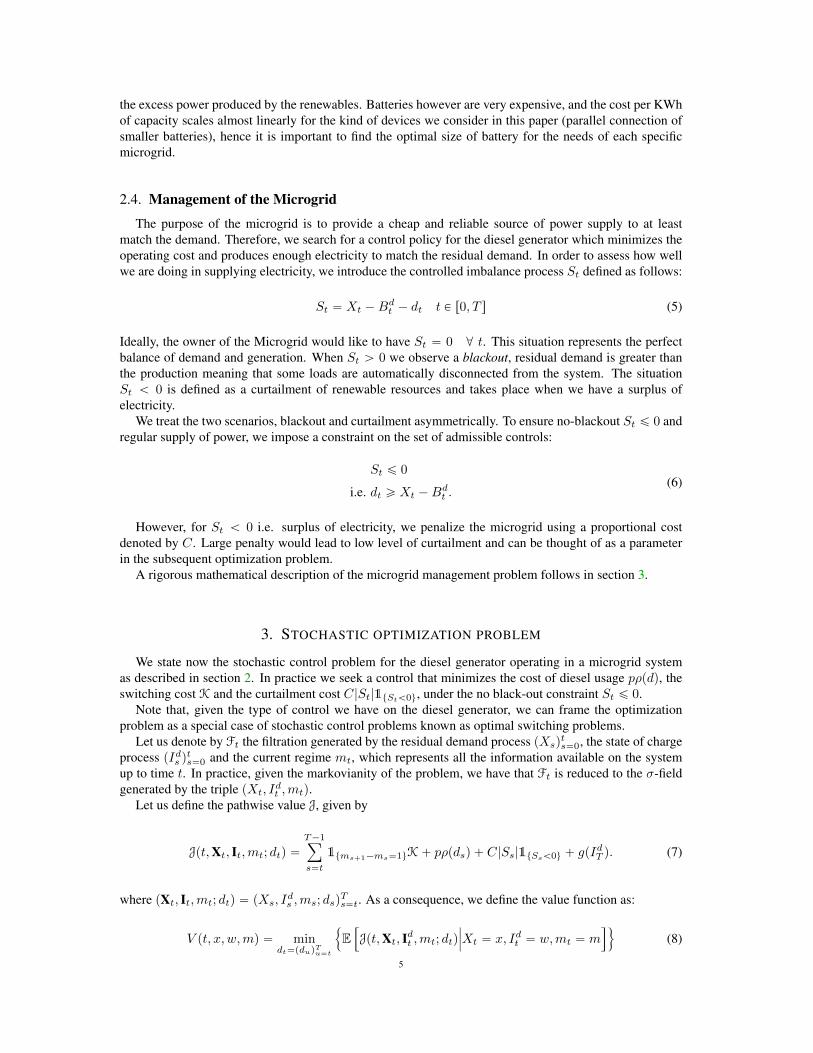
FIGURE 3. In the three panels above we display the estimated regression coefficients correspond-ing to the basis tx, i, x iu in the case of 2D regression, and txu at three different inventory levelsfor GD for mt “ 1. Although we used basis function up to polynomial degree 2, we present fewcoefficients for clarity of presentation. Notice that the time axis is inverted to show the numberof time steps computed backward. Remarkable smooth coefficients are computed by the RegressLater algorithm.
According to the parameters table above, and recalling remark 4 the residual demand has the followingdynamics:
Xt`1 “`
Xtp1´ 0.5∆tq ` σ?
∆tξt˘
^ 10, t P t0, 1, . . . , T ´ 1u, (12)
where ξt „ Np0, 1q.We decided to use such simple dynamics for illustrative purposes in order to make the sensitivity of the
optimal control policy to the remaining parameters more straight forward to understand.Consider now that for the parameters listed above, the problem is time homogeneous. We have also
observed empirically that the estimated continuation values tend to forget the terminal condition ratherquickly. We show in Figure 3 that the regression coefficients for all algorithms converge to a stationaryvalue time steps, suggesting that optimization ran for longer time horizons would not bring any noticeableeffect to control policy. Since all three methods use polynomial basis of degree two for the projection,it also allows for easy comparison of the dynamics of the coefficients across methods. For example, atinventory level I “ 0 the dynamics of the coefficient for x achieves same stationary level for both GridDiscretization and Regress Now. Although an exact comparison is not possible between Regress Now andRegress Later, we continue to observe similar sign and dynamics for each of the coefficients. However,getting away with almost no noise in the dynamics of the estimated coefficients of Regress Later comparedto Regress Now is essentially magical.
As a result, we define a stationary policy dpx,w,mq to be used in a longer time horizon than the oneemployed for its estimation which performance are comparable to the time dependent policy dpt, x, w,mq.
We finally tested the value of both stationary and time dependent policy and found that the performanceof the stationary policy is comparable to that of the time dependent policy.
5.1. Analysis of the controllers
In this section we compare the control policies estimated by the three algorithms and we try to assesswhether one of the approaches is preferable.
5.1.1. Control maps
We compare now the stationary control policies produced by the different algorithms; recall that thesepolicies are feedback to the state, i.e. can be written as function dmpx,wq. Figure 4 displays an exampleof the feedback control policy in the form of control map, a graphical representation of the value of theoptimal control for each pair px,wq.
We observed that the three policies agree with the intuition that the diesel generator should producemore power when residual demand is high and inventory is low. We can also notice that the switching costinfluences the policy, forcing the diesel to keep running for longer in order to charge the battery sufficientlyand avoid turning ON and OFF the generator too often. Just by observation of the control maps little
11

(A) (B) (C)
FIGURE 4. In the figure above we show, in the two left-most panels, an example of control mapproduced by the Regress Later algorithm. Notice the difference depending on the state of thegenerator. In the right-most panel we display the estimated probability density function of the stateof charge of the battery associated with the use of the three policies. It can be observed that RegressLater and Grid discretization induce very similar distributions.
difference can be found among the algorithms, we display in Figure 4 the effect of the control policy on athe state of charge of the battery. It can be observed from the estimated unconditional probability densityof the process I that the policies induced by Regress Now and Regress Later are very similar. Both seemto induce a peculiar mass of probability around In “ 2.5, differentiating the behavior of the inventorycompared to Grid Discretization. The distribution of the state of charge, obtained by plotting the histogramof all simulations over all time steps, shows that Regress Now and Regress Later does not fully exploitthe whole inventory but rather they are more conservative, saving energy to avoid to turn ON the dieselgenerator in the future. In the next section we will investigate the value associated to this control maps.
5.1.2. Performance of the policies
In order to assess the performance of each policy in an unbiased manner, we select a collection ofsimulated paths of the residual demand process X , and record the costs associated with managing themicrogrid as indicated by each control map.
We first study how the quality of each policy improves when we increase the computational budget givento each algorithm to compute the stationary policy. In Figure 5, we show the estimated value of the policywhen the initial state of the system is px, i,mq “ p0, 5, 0q for polynomial basis functions of increasingdegree, for 2D regression. In case of GD we increase the number of discretisation points for the inventory.In particular we make the computational time increase by providing the problem with more training pointsand more parameters to use in the definition of C as increasing the number of basis functions. In the case of2D regression, surprisingly, we noticed that the performance of the estimated control improves only whenpolynomials of even degree are added, and the effect is more prominent for Regress Later.
We notice from the comparison that Grid Discretisation converges quickly, resulting in the best algo-rithm in terms of trade off between running time and precision. Among the 2D regressions, we observesimilar bias for Regress Now and Regress Later (not displayed in order to maintain clear presentation, butavailable on request), however latter has lower standard error. This is not surprising because Regress Laterhas only one element of approximation error due to finite basis functions while Regress Now has error at-tributed to two sources, first, due to finite basis function and second, pathwise estimation of the conditionalexpectation.
5.2. System behavior
In the previous section we selected Grid Discretisation to be the best performing algorithm by ourcriteria. In the following we shall always employ Grid Discretisation to conduct our study of the sensitivityof the control policy and the associated cost of managing the grid to some of the parameters of the model.
The aim of the section is to build a solid understanding of the behavior of the microgrid in order to getan insight into the optimal design of the system. We decided to study the following aspects of the grid:battery capacity, represented by Imax; different proportion of renewable production, via the volatility σand the mean reversion b; tenable behavior of the policy, via the switching cost K and curtailment cost C.
12

FIGURE 5. The figure in display shows the reduction in operating cost when higher degree poly-nomials are added to the basis functions, in the case of RN regression, or more inventory pointsin Grid Discretisation. Notice the peculiar behavior of even/odd degree of basis functions in theRN regressions. Similar analysis was performed for Regress Later and the results are available onrequest.
FIGURE 6. In the figure above we show histograms for different levels of battery capacity. In thetop panel we display the estimated probability density of the curtailed energy, while in the bottompanel the estimated density of the cost of operating the diesel generator. Notice that the decreasein cost and curtailed energy per KWh of additional capacity is smaller for high capacity batteries.
In order to be able to carry out our analysis, without introducing cumbersome economic and engineeringdetails regarding the microgrid components, we have to make very simplistic assumptions. Our aim ishowever to guide the reader through a methodology that can be replicated to study real world microgridsystems.
5.2.1. Battery capacity
We study first the behaviour of the system relatively to changes in the capacity of the battery. Wewould expect to observe negative correlation between the quantity of diesel consumed and the battery size.We display in Figure 6 both the quantity of energy curtailed and the cost of running the diesel generatorfor different values of the battery capacity. We can observe that, as expected, increasing the size of thebattery leads to lower diesel usage thanks to the higher proportion of renewable energy that is retainedwithin the system. As the capacity of the battery reaches 30/40 KWh, we start observing a decrease in thecost-reduction per KWh of additional capacity suggesting that further analysis should be run in order tounderstand up to which size it is worth to pay to add storage capacity to the system.
We show now how to infer information about the optimal sizing of the battery, minimizing the tradeoff between the installation cost of a bigger battery and the reduced use of the diesel generator. Considerhowever that including battery ageing in the stochastic control problem is outside the scope of this paperbut rather in this section we present only a post-optimization analysis. Assuming that the microgrid runsunder similar conditions for the next 10 years, we can quickly estimate the total throughput of energy forthe different battery capacities. Consider now that a battery has not an infinite lifetime, but rather it should
13

FIGURE 7. In the figure above we compute the total cost of installing and running the grid for tenyears, assuming we replace the battery every 4000 cycles, and plot it against the battery capacity(left panel). From the corresponding minimum we can work out the optimal battery capacity and,further, compute the sensitivity of such result with respect to the cost per KWh of capacity.
be scrapped after equivalent 4000 cycles (amount of energy for one full charge and discharge). Underthe previous assumptions, we can compute how many batteries would be necessary to cover the next 10years of operations. Similarly, using the data relative to the usage of diesel generator for different levelsof capacity, we can compute the operating cost of the diesel generator over the same time period. Furtherexploiting the assumption about the lifetime of a battery, we obtain the cost of running the grid for 10 yearsas a function of the number of batteries. To conclude, assuming a linear cost of 400 e/KWh of capacity,we work out the installation cost of the different-size storage devices.
Once this information is collected we search for the minimum of the sum of installation and runningcost and, in turn, we compute the optimal capacity. Figure 7, on the left, displays a graphical summary ofthe procedure just described and shows that in our problem the optimal size of the battery is 14 KWh underthe current set of assumptions. Further, we study how much our result is affected by the cost per KWh ofcapacity, repeating the procedure above. We find that, as expected, as cost increase the size of the optimalbattery decreases. Figure 7, on the right, displays such behaviour.
5.2.2. Renewable penetration
In this section we want to investigate how robust the microgrid is to higher penetration of renewablegeneration, or, in other words, to what extent the algorithm can cope with increasing randomness anddecreasing predictability of the system. To model this phenomena we assume that greater penetration ofrenewables can be modeled by increasing both the parameters for volatility σ and the mean reversion rateλ. Increasing these two parameters makes the problem more difficult to solve, given that the control policycan rely less and less on the statistical properties of the process X .
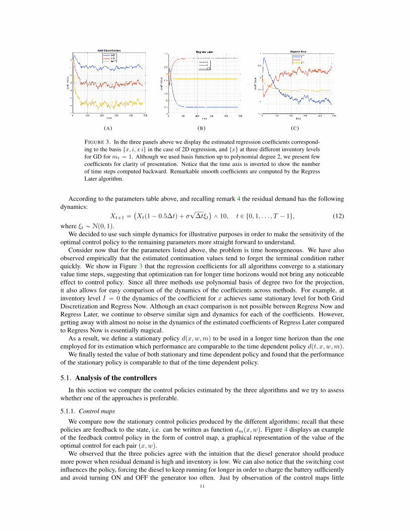
In order to establish the real added value provided by our stochastic optimization algorithm, we comparethe estimated policy with an heuristic myopic control which can be reproduced in our model solving thedynamic programming equation (10) taking constant conditional expectation with respect to the control.We show the value of the two control policies as function of the increasing learning difficulty in Figure 8where we observe that the value of accounting for statistical estimation of future conditional expectationswhen taking decisions decreases.
In figure 8 we present cost of diesel as a function of σ for stochastic and myopic policy. Since increasingσ alters the volatility of the distribution, we define the mean reversion rate λ :“ σ2{p2cq in order to ensurethat the volatility of the process is constant while we increase σ. The stochastic policy leads to at least12% reduction in the cost of the diesel usage, compared to the myopic policy, and the difference magnifieswith increasing “fluctuations" in the process. The decreasing relationship of the cost with σ signifies theimportance of the battery storage system in the microgrid which absorbs the sharp change in the demand.In figure 9 we compare the demand for two different levels of the σ, the dynamics of the diesel generatorand the inventory. Notice significantly less usage of the diesel for high fluctuations, σ “ 5, compared toσ “ 1.175.
14
FIGURE 8. The figure represents the cost of the diesel usage for stochastic and myopic policyas a function of σ. The orange curve represents the percentage improvement in cost due to as aproportion of cost of myopic policy.
(A) (B)
FIGURE 9. Figure in the left and right panel represents demand, diesel usage and the inventorydynamics for low and high σ respectively. It is important to mention that the mean reversion ratewas chosen as λ :“ σ2
{8, in order to ensure a constant volatility of the process regardless of σ.Notice the low usage of the diesel generator in the figure on the right compared to the one on theleft.
The results of this experiment are affected by the over-pessimistic assumption of modeling greater pen-etration of renewables with an increasingly unpredictable, and eventually completely random, residualdemand process. This sort of analysis can however provide insight into how much (weather and load)forecasting capability will be necessary for a given level of renewable penetration.
5.2.3. Switching and curtailment
We conclude this section by analyzing the dependence of the system behavior on two key parametersin the model: switching cost K and curtailment cost C. Switching cost is a system’s property and themicrogrid controller has little freedom over, however the controller can significantly reduce the amountof curtailed energy by choosing the appropriate curtailment cost. In figure 10, we observe that increasingthe curtailment cost reduces the total curtailed energy by approximately 4%. However, it comes at thecost of inefficient usage of the diesel generator, which is represented on the right in the figure 10. Thehistograms represent the difference between the cost of diesel usage (blue) and the energy curtailed (orange)for C=20 and C=2. Positive diesel cost depicts inefficient usage of the diesel at C=20 compared to C=2.Depending upon the specific cost functional for the diesel, the controller can use C as a parameter for betteroptimization.
15

-80 -60 -40 -20 0 20 40 60 80 100
cost/curtailed energy
0
0.02
0.04
0.06
0.08
0.1
0.12
0.14
0.16
cost of dieselenergy curtailed
2 4 6 8 10 12 14 16 18 20
curtailment Cost
0.955
0.96
0.965
0.97
0.975
0.98
0.985
0.99
0.995
1
ener
gy r
educ
tion
curtailmentdiesel
FIGURE 10. Line plot on the left, represents the impact of curtailment cost on the total curtailedenergy for different C as a proportion of curtailed energy at C=2. The histogram on the right,represents the difference in cost of diesel and the curtailed energy for C=20 and C=2. Notice theincrease in curtailment cost leads to reduced curtailed energy but at the expense of inefficient dieselusage.
(A) K “ 2 (B) K “ 5
FIGURE 11. Figure on the left represents the control map for switching cost K “ 2, while thefigure on the right represents the control map for K “ 5 when the generator is ON. Notice theincrease in area for light blue (corresponding to d “ 1) in the figure on the right because ofincreased switching cost.
The optimal policy when the generator is ON mt “ 1 is significantly altered depending upon theswitching cost. For example, in figure 11, we present the control maps associated with K=2 and K=5. Asexpected, larger switching cost disincentivise the controller to switch OFF the diesel generator once it’sON. However, we don’t observe "significant" change in the control policy due to increase in switching costwhen the generator is OFF.
6. COMPARISON WITH DETERMINISTICALLY TRAINED POLICY
In this section we compare our stochastic optimization algorithm with a deterministically trained policy.The latter is widely used in online optimization where the solution is computed with respect to the bestforecast available at a given time. We emulate this situation by computing the optimal set of actions for aparticular deterministic demand trajectory at different levels of the inventory. We assume that the forecastof the demand is given by:
Xt`1 “ Xt ` 0.5p6 sinpπt
12q ´Xtq∆t; t P t0, 1, . . . , T ´ 1u. (13)
16

(A) Demand (B) Inventory (C) Diesel Output
FIGURE 12. The image illustrates the dynamics of the inventory and control for the deterministiccontrol problem. Figure (A) represents the demand in equation (13), the optimal control of thediesel in figure (C) and the corresponding dynamics of the inventory in figure (B).
Equation (13) implies periodicity of one day in the residual demand and is equivalent to σ “ 0, b “ 0.5and Λt “ 6 sinpπt12 q1 in (2). Zero volatility in the residual demand curve leads to a deterministic optimalcontrol problem, rather than a stochastic control problem we have presented in section 5.
Notice that the deterministic optimal control problem results in a sequence of control maps dt : pw,mq Ñrdmin, dmaxs Y 0. As a result, although the policy has been trained on a deterministic residual demand,it dynamically adapts itself to different inventory levels and state of the diesel generator, when tested in astochastic environment. We present the modified algorithm in 4. There are two key differences from theprevious algorithm, first, we use one dimensional projection of the value function and second, we replaceregression with interpolation since there is no randomness left in the problem.
Algorithm 4 Regression Monte Carlo algorithm for deterministic demand
1: Simulate tXtuNt“1 according to its dynamics;
2: Discretize It into M levels indexed by j s.t. tIjt uMj“1 ;
3: Initialize the value function V pT, IjT ,mT q “ gpIjT q, @j “ 1, . . . , M and mT “ t0, 1u ;4: for t “ N ´ 1 to 1 do5: Find interpolation function Bpt` 1, It`1,mq for tV pt` 1, Ijt`1,mt`1qu
Mj“1 for each m “ 0, 1
6: Compute the set of admissible controls as Ut7: for j “ 1 to M do8: for m “ 0 to 1 do9: F “ Bpt` 1, Ijt , 0q
10:
V pt, Ijt ,mq “
$
’
&
’
%
mindPUtzt0u
!
pρpdq ` CSt1tStă0u `Bpt` 1, Ijt ´Bdt , 1q
)
`K1tm“0u ^ F if 0 P Ut
mindPUt
!
pρpdq ` CSt1tStă0u `Bpt` 1, Ijt ´Bdt , 1q
)
`K1tm“0u otherwise
output: control policy tBpt, ¨, ¨quNt“2.
In order to understand the solution of the deterministic problem, in figure 13 we present the dynamics ofthe optimal control and inventory corresponding to the demand faced in (A). As expected, diesel switcheson when the demand is high and it keeps it running just long enough that the battery is empty before itfaces negative residual demand to charge the battery. Moreover, there is substantial curtailment of energysince the battery is not large enough to store all the excess energy.
In order to quantify the gain due to formulating the microgrid management problem as a stochasticcontrol rather than traditional deterministic control, we compare the performance of the deterministicallytrained strategy of this section to its stochastic counterpart developed in this paper. While the deterministiccontrol problem was solved using the residual demand curve (13), the stochastic control problem was fedin with the residual demand curve (14). Finally, we test both the strategies on fresh out-of-sample paths
17

FIGURE 13. Difference of the Costof Stochastic and deterministic policyfor K=5
Switching Cost K=2 K=5 K=10Deterministic 138.56 162.63 201.52Stochastic 131.86 150.49 178.22% difference 4.84% 7.46% 11.56%
TABLE 1. Comparison of deter-ministic and stochastic trained pol-icy.
following the residual demand (14).
Xt`1 “
´
Xt ` 0.5p6 sinpπt
12q ´Xtq∆t` 2
?∆tξt
¯
^ 10 ; t P t0, 1, . . . , T ´ 1u (14)
In figure 13, we present the histogram of the cost from the stochastic policy and the deterministic policypathwise for 10,000 out-of-sample paths. As evident, most of the distribution lies on the negative side,implying gain due to stochastic policy. To measure this difference, in table 1, we quantify the gain of thestochastic policy for different switching cost. For switching cost of K=5, we observe that the stochasticpolicy is 7.5% better than the deterministic policy. As the switching cost increases, mistakes made bydeterministic policy become more expensive leading to higher percentage difference.
Finally, Figure 14 displays the behavior of inventory and the cost along a random trajectory of residualdemand. In blue we show the stochastically trained control policy and in orange the deterministicallytrained. The stochastic policy has lesser switch of the diesel generator and thus lower costs. The spikes inthe cost function for the deterministic policy is due to poor management of the inventory and thus inefficientusage of the microgrid.
7. CONCLUSION
In this paper we solved the problem of optimal management of a microgrid by employing three algo-rithms from the Regression Monte Carlo literature, namely: Regress Now, Regress Later and InventoryDiscretization. We find that Inventory Discretization significantly outperforms the other two methods. Be-sides algorithm design, we propose a methodology to optimize the design of the grid and determine theoptimal sizing of the battery. In addition, we perform a thorough sensitivity analysis to some of the keyparameters, showing the robustness of our solution. Finally, we compare the control policy estimated byour algorithm to industry standard deterministic control, observing a 5-10% reduction in cost.
Future research in this direction will include further studies of the optimal sizing of the battery by ex-plicitly incorporating the wearing off caused by usage. Another more challenging direction is to understandthe impact of delay, e.g., in the switching of the diesel generator, on the optimal management of the micro-grid. This problem introduces several mathematical and algorithmic issues which are currently the focusof our research.
8. ACKNOWLEDGEMENTS
This research was supported by the FIME Research Initiative. The research of C. Alasseur and X. Warinhas also benefited from support by the ANR project CAESARS (ANR-15-CE05- 0024). The research ofPeter Tankov has also benefited from support by the ANR project FOREWER (ANR-14-CE05- 0028). Theresearch of Aditya Maheshwari has benefited from support by the grant AMPS-1736439.
18

FIGURE 14. The figure above presents the pathwise comparison of stochastic and deterministicpolicy for the same demand on the left panel. The center panel represents dynamics of the inventorydue to control on the right panel. Particularly notice the difference in switching times for the dieselin the deterministic policy and stochastic policy.
19
REFERENCES
[1] A. Balata and J. Palczewski. Regress-Later Monte Carlo for Optimal Inventory Control with applications in energy. ArXive-prints, March 2017.
[2] Alexander Boogert and Cyriel de Jong. Gas storage valuation using a monte carlo method. The Journal of Derivatives, pages81–98, March 2008.
[3] Bruno Bouchard and Xavier Warin. Monte-carlo valuation of american options: facts and new algorithms to improve existingmethods. In Numerical methods in finance, pages 215–255. Springer, 2012.
[4] René Carmona and Michael Ludkovski. Valuation of energy storage: an optimal switching approach. Quantitative Finance,10(4):359–374, 2010.
[5] Jérôme Collet, Olivier Féron, and Peter Tankov. Optimal management of a wind power plant with storage capacity. HAL preprinthal-01627593, 2017.
[6] Huajie Ding, Zechun Hu, and Yonghua Song. Stochastic optimization of the daily operation of wind farm and pumped-hydro-storage plant. Renewable Energy, 48:571–578, 2012.
[7] Huajie Ding, Zechun Hu, and Yonghua Song. Rolling optimization of wind farm and energy storage system in electricitymarkets. IEEE Transactions on Power Systems, 30(5):2676–2684, 2015.
[8] Hugo Gevret, Jerome Lelong, and Xavier Warin. STochastic OPTimization library in C++. Research report, EDF Lab, September2016.
[9] Pierre Haessig, Bernard Multon, Hamid Ben Ahmed, Stéphane Lascaud, and Pascal Bondon. Energy storage sizing for windpower: impact of the autocorrelation of day-ahead forecast errors. Wind Energy, 18(1):43–57, 2015.
[10] Naoki Hayashi, Masaaki Nagahara, and Yutaka Yamamoto. Robust ac voltage regulation of microgrids in islanded mode withsinusoidal internal model. SICE Journal of Control, Measurement, and System Integration, 10(2):62–69, 2017.
[11] B. Heymann, J. F. Bonnans, F. Silva, and G. Jimenez. A stochastic continuous time model for microgrid energy management. In2016 European Control Conference (ECC), pages 2084–2089, June 2016.
[12] Benjamin Heymann, J. Frédéric Bonnans, Pierre Martinon, Francisco J. Silva, Fernando Lanas, and Guillermo Jiménez-Estévez.Continuous optimal control approaches to microgrid energy management. Energy Systems, Jan 2017.
[13] Hao Liang and Weihua Zhuang. Stochastic modeling and optimization in a microgrid: A survey. Energies, 7(4):2027–2050,2014.
[14] S. Mashayekh, M. Stadler, G. Cardoso, M. Heleno, S. Chalil Madathil, H. Nagarajan, R. Bent, M. Mueller-Stoffels, X. Lu, andJ. Wang. Security-constrained design of isolated multi-energy microgrids. IEEE Transactions on Power Systems, PP(99):1–1,2017.
[15] Salman Mashayekh, Michael Stadler, Gonçalo Cardoso, and Miguel Heleno. A mixed integer linear programming approach foroptimal der portfolio, sizing, and placement in multi-energy microgrids. Applied Energy, 187(Supplement C):154 – 168, 2017.
[16] Lanre Olatomiwa, Saad Mekhilef, A.S.N. Huda, and Olayinka S. Ohunakin. Economic evaluation of hybrid energy systems forrural electrification in six geo-political zones of nigeria. Renewable Energy, 83(Supplement C):435 – 446, 2015.
[17] Daniel E Olivares, Ali Mehrizi-Sani, Amir H Etemadi, Claudio A Cañizares, Reza Iravani, Mehrdad Kazerani, Amir HHajimiragha, Oriol Gomis-Bellmunt, Maryam Saeedifard, Rodrigo Palma-Behnke, et al. Trends in microgrid control. IEEETransactions on smart grid, 5(4):1905–1919, 2014.
[18] S. Surender Reddy, Vuddanti Sandeep, and Chan-Mook Jung. Review of stochastic optimization methods for smart grid.Frontiers in Energy, 11(2):197–209, Jun 2017.
[19] Xavier Warin. Gas Storage Hedging, pages 421–445. Springer Berlin Heidelberg, Berlin, Heidelberg, 2012.
20