Regression Models for Time Trends

INSR 260, Spring 2009Bob Stine

1

Overview Review categorical variables

Polynomial trends

Seasonal patterns via indicators

Testing for omitted patterns: Durbin-Watson

Prediction

Example!! ! ! (from Bowerman, Ch 6)Planning staffing levels for a seasonal business:Hotel occupancyOther examples in Chapter 6 Time Series Regression

2

Categorical VariablesTwo special types of explanatory variables

IndicatorsShift the regression line up or down by altering the intercept of the fitted model for cases in a subset

InteractionsAlter the slope for a particular group, capturing different levels of association between y and x within subsets

Particularly relevant test: Partial F-testUsed in general to test whether a subset of slopes in a regression model are zeroTest whether the slopes (interaction) or the intercepts (categorical slopes) differ among the groups

3

Forecasting ProblemPredict occupancy rates for hotel

14 years of monthly data, n = 168Forecast occupancy during the next yearProvide a measure of the forecast accuracy

Evident patternsGrowthSeasonalVariation

Color-coding can also help verify the seasonality4

500

600

700

800

900

1000

1100

Occupied

0 50 100 150

Time

Overlay Plot

Table 6.4

Modeling ApproachDecomposition! ! ! ! ! ! ! ! ! ! (also in Ch 7)! ! Data = Trend + Seasonal + Irregular

TrendSimple functions of time that are easily forecasted, such as linear or quadratic growth

SeasonalRepeating patterns, such as those related to weather or holidays

IrregularMay be dependent and predictable

5

Initial ModelingLinear trend + Monthly seasonal pattern

Multiple regression with time trend (month = 1,2,3...)and monthly dummy variables (11 indicators, dec omitted)

Overall fit is highly statistically significant

Specific coefficients by-and-large differ

6

RSquare

RSquare Adj

Root Mean Square Error

Mean of Response

Observations (or Sum Wgts)

0.978941

0.977311

21.48822

722.2976

168

Summary of Fit

Model

Error

C. Total

Source

12

155

167

DF

3327046.9

71570.2

3398617.1

Sum of

Squares

277254

462

Mean Square

600.4501

F Ratio

<.0001*Prob > F

Analysis of Variance

Time

Month

Source

1

11

Nparm

1

11

DF

1499569.3

1771253.7

Sum of

Squares

3247.624

348.7284

F Ratio

<.0001*

<.0001*

Prob > F

E!ect Tests

Intercept

Time

Month[Jan]

Month[Feb]

Month[Mar]

Month[Apr]

Month[May]

Month[Jun]

Month[Jul]

Month[Aug]

Month[Sep]

Month[Oct]

Month[Nov]

Term

518.86538

1.953083

-27.01609

-71.82631

-56.13654

25.267521

12.671581

106.43278

229.19399

250.66947

38.216392

27.406166

-74.11835

Estimate

6.518866

0.034272

8.130527

8.12901

8.127637

8.126409

8.125325

8.124385

8.12359

8.122939

8.122433

8.122072

8.121855

Std Error

155.00

155.00

155.00

155.00

155.00

155.00

155.00

155.00

155.00

155.00

155.00

155.00

155.00

DFDen

79.59

56.99

-3.32

-8.84

-6.91

3.11

1.56

13.10

28.21

30.86

4.71

3.37

-9.13

t Ratio

<.0001*

<.0001*

0.0011*

<.0001*

<.0001*

0.0022*

0.1209

<.0001*

<.0001*

<.0001*

<.0001*

0.0009*

<.0001*

Prob>|t|

Indicator Function Parameterization

Residual DiagnosticsSubstantial pattern was missed

Big R2 does not guarantee a “good” model

Two residual plots are essential when have time series data: ! - familiar plot of e on ŷ ! - sequence plot of the residuals

7

-70

-50

-30

-10

10

30

50

70

Occupie

d R

esid

ual

500 600 700 800 900 1000

Occupied Predicted

-70

-50

-30

-10

10

30

50

70

Resid

ual

0 20 40 60 80 100 120 140 160

Row Number

Two Ways to FixTwo approaches

Add interactions that allow slopes to differ by seasonTransform the response to stabilize the variance

Log transformationNatural log (base e)

8

6.1

6.2

6.3

6.4

6.5

6.6

6.7

6.8

6.9

7

Log O

ccupie

d

0 50 100 150

Time

Overlay Plot

Can also show original on log scale (better

for presenting)

Revised ModelVery impressive fit overall (on log scale)

Do NOT compare R2 statistic to prior model since the response variable is not the same as in the prior model

Interpretation of slope for timeRate of growth: about 0.3% per month

Interpretation of dummy variablesShift intercept relative to December

9

RSquare

RSquare Adj

Root Mean Square Error

Mean of Response

Observations (or Sum Wgts)

0.988665

0.987787

0.021186

6.563887

168

Summary of Fit

Intercept

Time

Month[Jan]

Month[Feb]

Month[Mar]

Month[Apr]

Month[May]

Month[Jun]

Month[Jul]

Month[Aug]

Month[Sep]

Month[Oct]

Month[Nov]

Term

6.2875573

0.0027253

-0.041606

-0.112079

-0.084459

0.0398331

0.0203951

0.1469094

0.2890226

0.3111946

0.0559872

0.0395438

-0.112215

Estimate

0.006427

3.379e-5

0.008016

0.008015

0.008013

0.008012

0.008011

0.00801

0.008009

0.008009

0.008008

0.008008

0.008008

Std Error

155.00

155.00

155.00

155.00

155.00

155.00

155.00

155.00

155.00

155.00

155.00

155.00

155.00

DFDen

978.26

80.65

-5.19

-13.98

-10.54

4.97

2.55

18.34

36.09

38.86

6.99

4.94

-14.01

t Ratio

<.0001*

<.0001*

<.0001*

<.0001*

<.0001*

<.0001*

0.0119*

<.0001*

<.0001*

<.0001*

<.0001*

<.0001*

<.0001*

Prob>|t|

Indicator Function Parameterization

Residual DiagnosticsPattern remaining?

How should the model be improved - if at all?What types of variables are missing from the model?What is a simple revision of the model?

Note: text does not revise the model10

-0.07

-0.06

-0.05

-0.04

-0.03

-0.02

-0.010.00

0.01

0.02

0.03

0.04

0.05

0.06Log O

ccupie

d

Resid

ual

6.1 6.2 6.3 6.4 6.5 6.6 6.7 6.8 6.9 7.0 7.1

Log Occupied Predicted

Residual by Predicted Plot

-0.07

-0.06

-0.05

-0.04

-0.03

-0.02

-0.01

0.00

0.01

0.02

0.03

0.04

0.05

0.06

Resid

ual

0 20 40 60 80 100 120 140 160 180

Row Number

Residual by Row Plot

Revised ModelModel with an additional quadratic component

Suggests rate of growth is slowingStatistically significant improvement?

Further structure?

11

RSquare

RSquare Adj

Root Mean Square Error

Mean of Response

Observations (or Sum Wgts)

0.989874

0.989019

0.02009

6.563887

168

Summary of Fit

Intercept

Time

Time*Time

Month[Jan]

Month[Feb]

Month[Mar]

Month[Apr]

Month[May]

Month[Jun]

Month[Jul]

Month[Aug]

Month[Sep]

Month[Oct]

Month[Nov]

Term

6.2724878

0.0032592

-3.159e-6

-0.041606

-0.112111

-0.084516

0.0397572

0.0203067

0.1468146

0.2889278

0.3111061

0.0559114

0.039487

-0.112247

Estimate

0.007035

0.000129

7.369e-7

0.007601

0.0076

0.007599

0.007598

0.007597

0.007596

0.007595

0.007594

0.007594

0.007593

0.007593

Std Error

154.00

154.00

154.00

154.00

154.00

154.00

154.00

154.00

154.00

154.00

154.00

154.00

154.00

154.00

DFDen

891.55

25.35

-4.29

-5.47

-14.75

-11.12

5.23

2.67

19.33

38.04

40.97

7.36

5.20

-14.78

t Ratio

<.0001*

<.0001*

<.0001*

<.0001*

<.0001*

<.0001*

<.0001*

0.0083*

<.0001*

<.0001*

<.0001*

<.0001*

<.0001*

<.0001*

Prob>|t|

Indicator Function Parameterization

-0.06

-0.05-0.04

-0.03

-0.02-0.01

0.000.01

0.02

0.030.04

0.05

Log O

ccupie

d

Resid

ual

6.1 6.2 6.3 6.4 6.5 6.6 6.7 6.8 6.9 7.0 7.1

Log Occupied Predicted

Residual by Predicted Plot

-0.06

-0.05

-0.04

-0.03

-0.02

-0.01

0.00

0.01

0.02

0.03

0.04

0.05Resid

ual

0 20 40 60 80 100 140 180

Row Number

Residual by Row Plot

Testing Residual DependenceDurbin-Watson test

Test whether adjacent residuals appear dependentTest related to autocorrelation between residuals

Autocorrelation is correlation between “rows” in the data table, whereas the usual correlation is between “columns”

Lag plot of residuals

Regression summary

12

-0.06

-0.05

-0.04

-0.03

-0.02

-0.01

0

0.01

0.02

0.03

0.04

0.05

Resid

ual

Log O

ccupie

d

-0.06 -0.04 -0.02 0 0.01 0.03 0.05

Lag Residuals

Residual Log Occupied = 0.000194 + 0.3257149*Lag

Residuals

RSquare

RSquare Adj

Root Mean Square Error

Mean of Response

Observations (or Sum Wgts)

0.103026

0.09759

0.018336

0.000105

167

Summary of Fit

Intercept

Lag Residuals

Term

0.000194

0.3257149

Estimate

0.001419

0.074819

Std Error

0.14

4.35

t Ratio

0.8914

<.0001*

Prob>|t|

Parameter Estimates

Linear Fit

et

et-1

1.3322276

Durbin-

Watson

168

Number

of Obs.

0.3147

AutoCorrelation

<.0001*

Prob<DW

Durbin-Watson

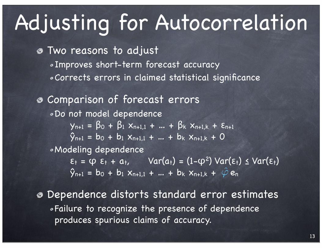
Adjusting for AutocorrelationTwo reasons to adjust

Improves short-term forecast accuracyCorrects errors in claimed statistical significance

Comparison of forecast errorsDo not model dependence! yn+1 = β0 + β1 xn+1,1 + … + βk xn+1,k + εn+1! ŷn+1 = b0 + b1 xn+1,1 + … + bk xn+1,k + 0Modeling dependence! εt = φ εt + at, !! Var(at) = (1-φ2) Var(εt) ≤ Var(εt)! ŷn+1 = b0 + b1 xn+1,1 + … + bk xn+1,k + en

Dependence distorts standard error estimatesFailure to recognize the presence of dependence produces spurious claims of accuracy.

13

!̂

Simple AdjustmentAdd the lagged residuals from the current model as an explanatory variable

Text describes more elaborate methods (p 311)

Residual plots show little remaining structureOther variables are still missing. Are these important?We’ll ignore them for the moment and build forecasts.Durbin-Watson is always OK after this correction

14

RSquare

RSquare Adj

Root Mean Square Error

Mean of Response

Observations (or Sum Wgts)

0.990798

0.989951

0.019085

6.565967

167

Summary of Fit

Intercept

Time

Time*Time

Month[Jan]

Month[Feb]

Month[Mar]

Month[Apr]

Month[May]

Month[Jun]

Month[Jul]

Month[Aug]

Month[Sep]

Month[Oct]

Month[Nov]

Lag Residuals

Term

6.2736436

0.0032199

-2.932e-6

-0.039028

-0.112117

-0.084519

0.0397564

0.0203076

0.1468168

0.2889308

0.3111094

0.0559145

0.0394895

-0.112245

0.328304

Estimate

0.006752

0.000125

7.116e-7

0.007362

0.00722

0.007219

0.007217

0.007216

0.007216

0.007215

0.007214

0.007214

0.007214

0.007213

0.078043

Std Error

152.00

152.00

152.00

152.00

152.00

152.00

152.00

152.00

152.00

152.00

152.00

152.00

152.00

152.00

152.00

DFDen

929.09

25.80

-4.12

-5.30

-15.53

-11.71

5.51

2.81

20.35

40.05

43.12

7.75

5.47

-15.56

4.21

t Ratio

<.0001*

<.0001*

<.0001*

<.0001*

<.0001*

<.0001*

<.0001*

0.0055*

<.0001*

<.0001*

<.0001*

<.0001*

<.0001*

<.0001*

<.0001*

Prob>|t|

Indicator Function Parameterization

!̂

ForecastingForecast log occupancy several periods outŷn+j = (6.2736 + bj) + !! ! ! ! ! ! ! ! ! seasonal! ! 0.00322 (n+j) - 0.00000293(n+j)2 +! ! time trend! ! 0.328j (en)!! ! ! ! ! ! ! ! ! ! ! autocorrAutocorrelation effect drops off geometrically, having little influence past a few terms

Point estimates for January, Februaryŷ168+1 = (6.2736-0.0390) + ! ! 0.00322 (169) - 0.00000293(169)2 +! !! ! 0.328 (0.0456)! ! ≈ 6.2346 + 0.4605 + 0.0150 = 6.7101ŷ168+2 = (6.2736-0.1121) + ! ! 0.00322 (170) - 0.00000293(170)2 +! !! ! 0.3282 (0.0456)! ! ≈ 6.1615 + 0.4627 + 0.0049 = 6.6291

15

Forecast AccuracyMore accurate in the near term because of the dependence between adjacent errors

Benefit of autocorrelation decreases as extrapolate outMust trick JMP into making the correct intervalsFollowing are approximate intervals; JMP shown next

One period out: use RMSE of fitted modelŷ168+1 ± t.025,152 RMSE != 6.7101 ± 1.98 (0.0191)! ! ! ! ! ! ! ! ≈ 6.6723 to 6.7479

Two periods out: inflate RMSE by sqrt(1+ 2)ŷ168+2±t.025,152RMSE(1+ 2)1/2 = 6.6291±1.98(0.0191)(1+.3282)1/2! ! ! ! ! ! ! ! ! ≈ 6.589 to 6.669

m periods out: inflate RMSE by ! ! sqrt(1 + 2 + 4 + … + 2(m-1) ≈ sqrt(1/(1- 2))

16!̂ !̂ !̂ !̂

!̂!̂

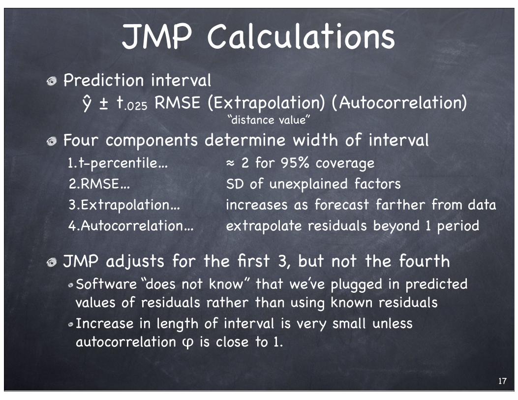
JMP CalculationsPrediction interval! ŷ ± t.025 RMSE (Extrapolation) (Autocorrelation)

Four components determine width of interval1.t-percentile… ! ! ! ≈ 2 for 95% coverage2.RMSE… ! ! ! ! ! SD of unexplained factors3.Extrapolation… !! ! increases as forecast farther from data4.Autocorrelation… ! ! extrapolate residuals beyond 1 period

JMP adjusts for the first 3, but not the fourthSoftware “does not know” that we’ve plugged in predicted values of residuals rather than using known residualsIncrease in length of interval is very small unless autocorrelation φ is close to 1.

17

“distance value”

JMP Calculations, cntdThe autocorrelation adjustment is the square root of the expression on the bottom of slide 16

This portion of the data table for hotel occupancy shows the data and columns.

18

Estimated future residual sqrt(1+phi^2) Slightly wider

!1 + !̂2 + !̂4 + ... + !̂2(m!1)

Prediction IntervalsWe need predictions of the occupancy, not the log of the occupancy

Predictions from model are on a log scale

ConversionForm interval as we have done on transformed scaleThen “undo” the transformation (here, exponentiate)

! ! 6.6695 to 6.7479! ! ⇒!! e6.6723 to e6.7506

! ! ! ! ! ! ! ! ! ! ! ! 790 to 855 rooms

Interval is much wider than you may have expected from the R2 and RMSE of model

Differences get far larger when exponentiate

19

Summary Polynomial trends are useful when lack other, substantive explanatory variables

Be cautious extrapolating a trend

Dummy variables model regular seasonal effects, but the magnitude of the variation often increases with the level

Log transformation stabilizes the variation and captures geometric growth

Durbin-Watson statistic tests for presence of autocorrelation in underlying model errors

20