Lecture 16: Generalized Additive Models

http://polisci.msu.edu/jacoby/icpsr/regress3

Regression III:Advanced Methods

Bill JacobyMichigan State University

2

Goals of the Lecture

• Introduce Additive Models

– Explain how they extend from simple nonparametric regression (i.e., local polynomial regression)

– Discuss estimation using backfitting

– Explain how to interpret their results

• Conclude with some examples of Additive Models applied to real social science data

3

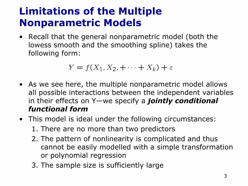
Limitations of the Multiple Nonparametric Models

• As we see here, the multiple nonparametric model allows all possible interactions between the independent variables in their effects on Y—we specify a jointly conditional functional form

• This model is ideal under the following circumstances:1. There are no more than two predictors2. The pattern of nonlinearity is complicated and thus

cannot be easily modelled with a simple transformation or polynomial regression

3. The sample size is sufficiently large

• Recall that the general nonparametric model (both the lowess smooth and the smoothing spline) takes the following form:

4

Limitations of the Multiple Nonparametric Models (2)• The general nonparametric model becomes impossible to

interpret and unstable as we add more explanatory variables, however

1. For example, in the lowess case, as the number of variables increases, the window span must become wider in order to ensure that each local regression has enough cases This process can create significant bias (the curve becomes too smooth)

2. It is impossible to interpret general nonparametric regression when there are more than two variables—there are no coefficients, and we cannot graph effects more than three dimensions

• These limitations lead us to the Additive Models

5

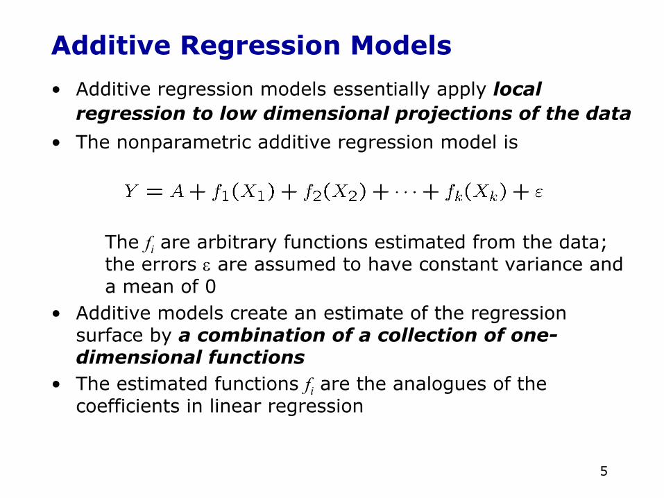
Additive Regression Models

• Additive regression models essentially apply local regression to low dimensional projections of the data

• The nonparametric additive regression model is

The fi are arbitrary functions estimated from the data; the errors ε are assumed to have constant variance and a mean of 0

• Additive models create an estimate of the regression surface by a combination of a collection of one-dimensional functions

• The estimated functions fi are the analogues of the coefficients in linear regression

6

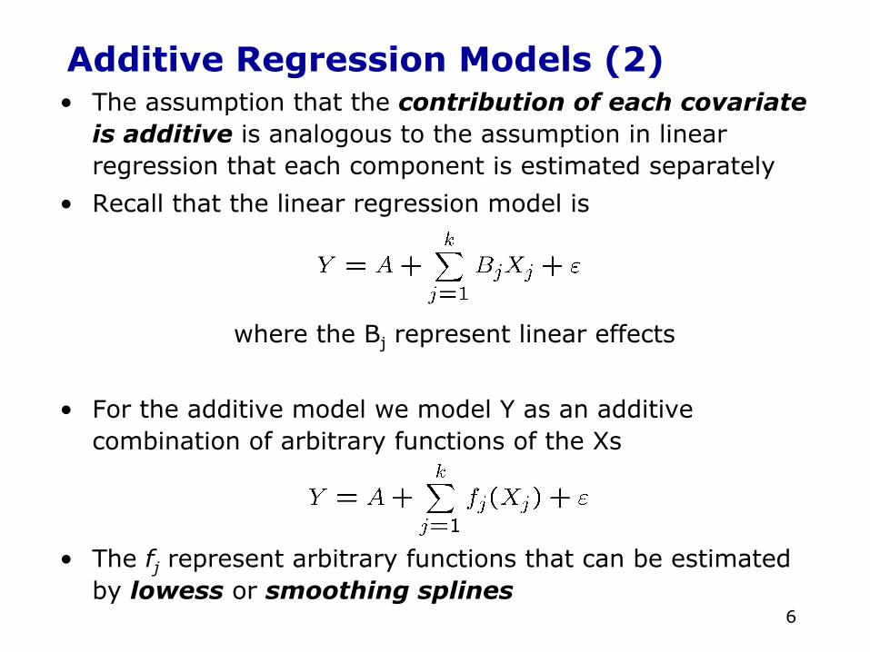
• The assumption that the contribution of each covariate is additive is analogous to the assumption in linear regression that each component is estimated separately

• Recall that the linear regression model is

Additive Regression Models (2)

where the Bj represent linear effects

• For the additive model we model Y as an additive combination of arbitrary functions of the Xs

• The fj represent arbitrary functions that can be estimated by lowess or smoothing splines

7

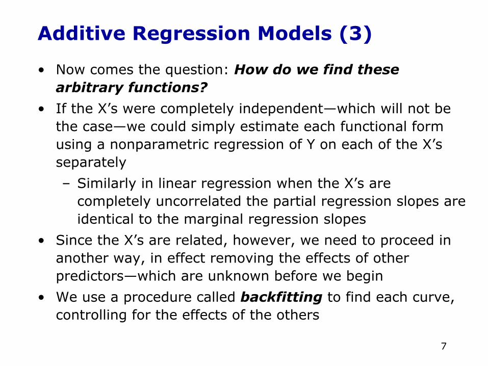
• Now comes the question: How do we find these arbitrary functions?

• If the X’s were completely independent—which will not be the case—we could simply estimate each functional form using a nonparametric regression of Y on each of the X’s separately

– Similarly in linear regression when the X’s are completely uncorrelated the partial regression slopes are identical to the marginal regression slopes

• Since the X’s are related, however, we need to proceed in another way, in effect removing the effects of other predictors—which are unknown before we begin

• We use a procedure called backfitting to find each curve, controlling for the effects of the others

Additive Regression Models (3)

8

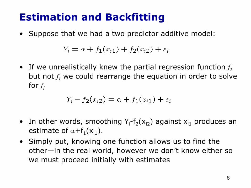
Estimation and Backfitting

• Suppose that we had a two predictor additive model:

• If we unrealistically knew the partial regression function f2but not f1 we could rearrange the equation in order to solve for f1

• In other words, smoothing Yi-f2(xi2) against xi1 produces an estimate of α+f1(xi1).

• Simply put, knowing one function allows us to find the other—in the real world, however we don’t know either so we must proceed initially with estimates

9

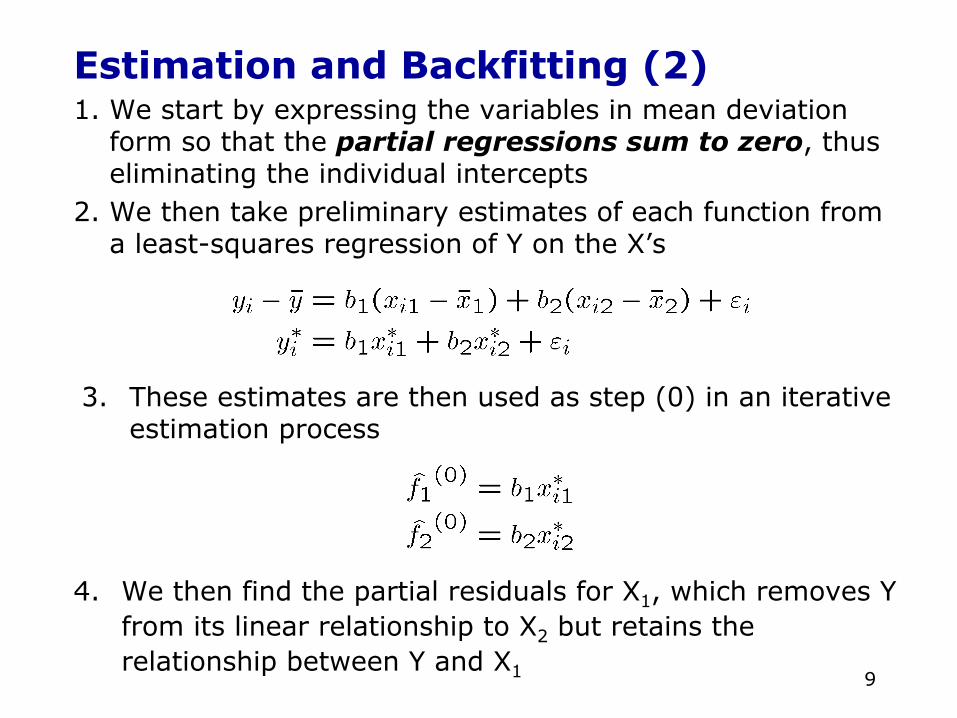
Estimation and Backfitting (2)1. We start by expressing the variables in mean deviation

form so that the partial regressions sum to zero, thus eliminating the individual intercepts

2. We then take preliminary estimates of each function from a least-squares regression of Y on the X’s

4. We then find the partial residuals for X1, which removes Y from its linear relationship to X2 but retains the relationship between Y and X1

3. These estimates are then used as step (0) in an iterative estimation process

10

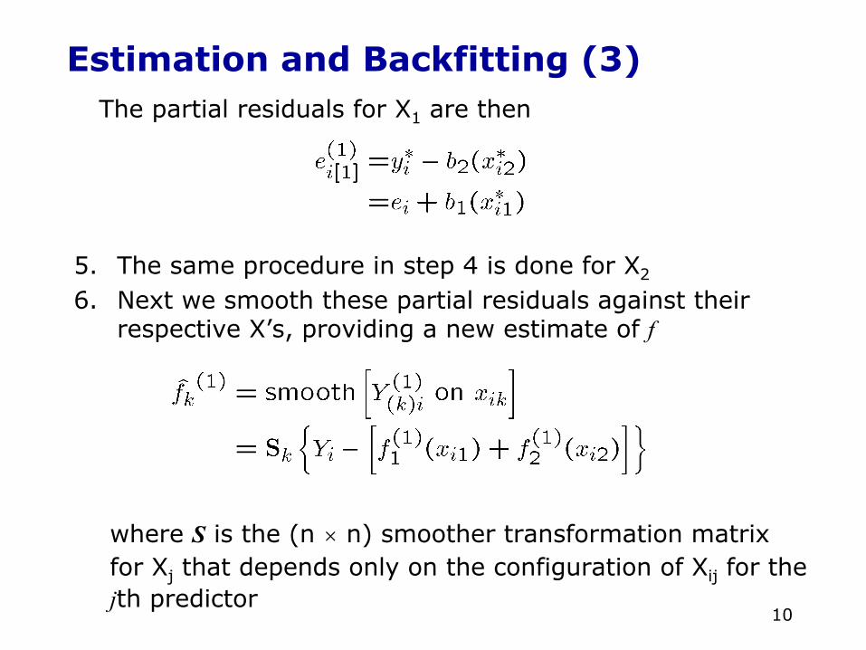
Estimation and Backfitting (3)The partial residuals for X1 are then

where S is the (n × n) smoother transformation matrix for Xj that depends only on the configuration of Xij for the jth predictor

5. The same procedure in step 4 is done for X2

6. Next we smooth these partial residuals against their respective X’s, providing a new estimate of f

11

Estimation and Backfitting (4)• This process of finding new estimates of the functions by

smoothing the partial residuals is reiterated until the partial functions converge– That is, when the estimates of the smooth functions

stabilize from one iteration to the next we stop• When this process is done, we obtain estimates of sj(Xij) for

every value of Xj

• More importantly, we will have reduced a multiple regression to a series of two-dimensional partial regression problems, making interpretation easy:– Since each partial regression is only two-dimensional,

the functional forms can be plotted on two-dimensional plots showing the partial effects of each Xj on Y

– In other words, perspective plots are no longer necessary unless we include an interaction between two smoother terms

12

Interpreting the Effects• A plot of of Xj versus sj(Xj) shows the relationship between

Xj and Y holding constant the other variables in the model• Since Y is expressed in mean deviation form, the smooth

term sj(Xj) is also centered and thus each plot represents how Y changes relative to its mean with changes in X

• Interpreting the scale of the graphs then becomes easy:– The value of 0 on the Y-axis is the mean of Y– As the line moves away from 0 in a negative direction

we subtract the distance from the mean when determining the fitted value. For example, if the mean is 45, and for a particular X-value (say x=15) the curve is at sj(Xj)=4, this means the fitted value of Y controlling for all other explanatory variables is 45+4=49.

– If there are several nonparametric relationships, we can add together the effects on the two graphs for any particular observation to find its fitted value of Y

13

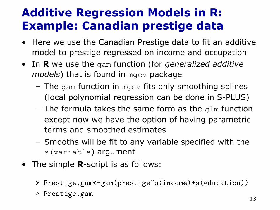
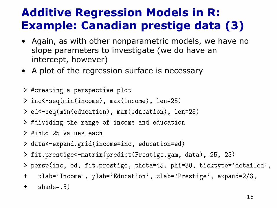
Additive Regression Models in R:Example: Canadian prestige data• Here we use the Canadian Prestige data to fit an additive

model to prestige regressed on income and occupation• In R we use the gam function (for generalized additive

models) that is found in mgcv package

– The gam function in mgcv fits only smoothing splines(local polynomial regression can be done in S-PLUS)

– The formula takes the same form as the glm function except now we have the option of having parametric terms and smoothed estimates

– Smooths will be fit to any variable specified with the s(variable) argument

• The simple R-script is as follows:

14

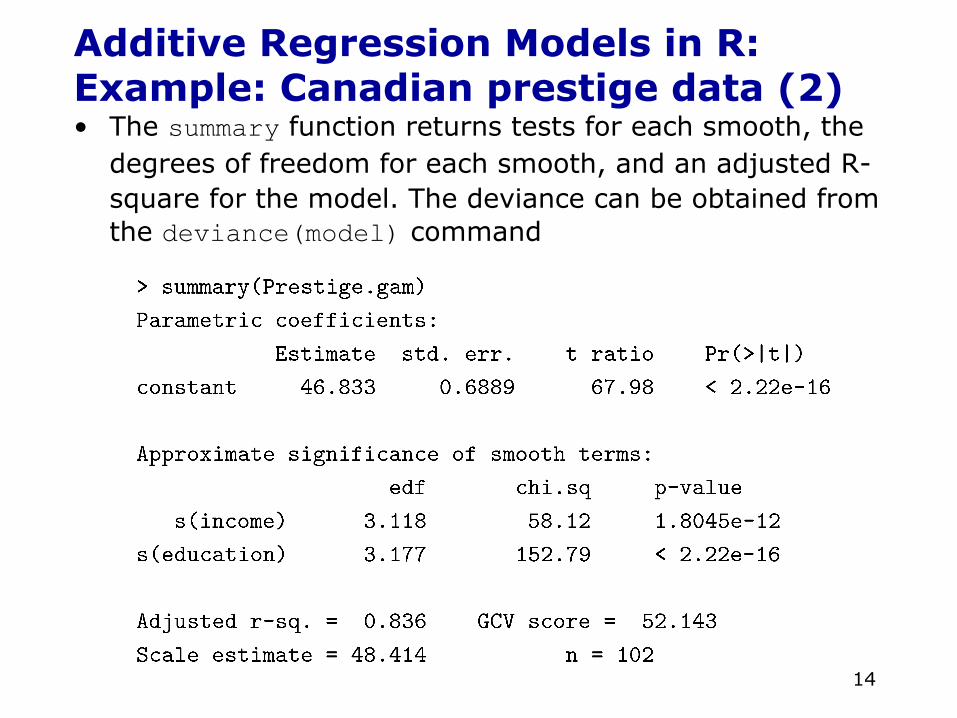
Additive Regression Models in R:Example: Canadian prestige data (2)• The summary function returns tests for each smooth, the

degrees of freedom for each smooth, and an adjusted R-square for the model. The deviance can be obtained from the deviance(model) command

15

Additive Regression Models in R:Example: Canadian prestige data (3)• Again, as with other nonparametric models, we have no

slope parameters to investigate (we do have an intercept, however)

• A plot of the regression surface is necessary

16

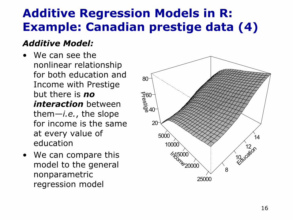
Additive Regression Models in R:Example: Canadian prestige data (4)Additive Model:• We can see the

nonlinear relationship for both education and Income with Prestige but there is no interaction between them—i.e., the slope for income is the same at every value of education

• We can compare this model to the general nonparametric regression model

Income

500010000

15000

20000

25000

Educat

ion

8

10

1214

Prestige

20

40

60

80

17

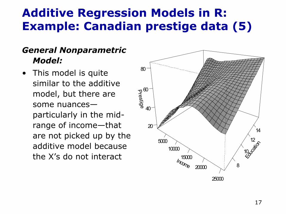
Additive Regression Models in R:Example: Canadian prestige data (5)

General Nonparametric Model:

• This model is quite similar to the additive model, but there are some nuances—particularly in the mid-range of income—that are not picked up by the additive model because the X’s do not interact Income

500010000

15000

20000

25000

Educ

ation

8

10

12

14

Prestige

20

40

60

80

18

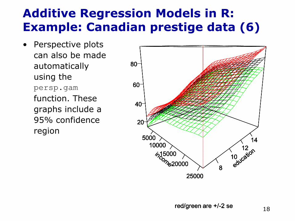
Additive Regression Models in R:Example: Canadian prestige data (6)• Perspective plots

can also be made automatically using the persp.gamfunction. These graphs include a 95% confidence region

income

500010000

1500020000

25000

education

8

1012

14

20

40

60

80

red/green are +/-2 se

income

500010000

1500020000

25000

education

8

1012

14

20

40

60

80

red/green are +/-2 se

income

500010000

1500020000

25000

education

8

1012

14

20

40

60

80

red/green are +/-2 se

income

500010000

1500020000

25000

education

8

1012

14

20

40

60

80

red/green are +/-2 se

19

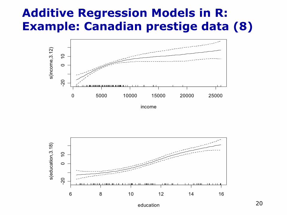
Additive Regression Models in R:Example: Canadian prestige data (7)• Since the slices of the additive regression in the

direction of one predictor (holding the other constant) are parallel, we can graph each partial-regression function separately

• This is the benefit of the additive model—we can graph as many plots as there are variables, and allowing us to easily visualize the relationships

• In other words, a multidimensional regression has been reduced to a series of two-dimensional partial-regression plots

• To get these in R:

20

Additive Regression Models in R:Example: Canadian prestige data (8)

0 5000 10000 15000 20000 25000

-20

010

income

s(in

com

e,3.

12)

6 8 10 12 14 16

-20

010

education

s(ed

ucat

ion,

3.18

)

21

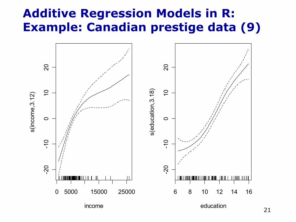
Additive Regression Models in R:Example: Canadian prestige data (9)

0 5000 15000 25000

-20

-10

010

20

income

s(in

com

e,3.

12)

6 8 10 12 14 16

-20

-10

010

20

education

s(ed

ucat

ion,

3.18

)

22

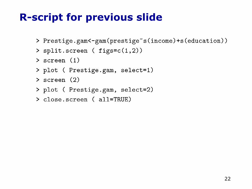
R-script for previous slide

23

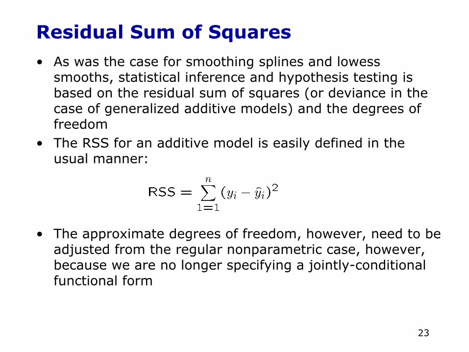
Residual Sum of Squares

• As was the case for smoothing splines and lowesssmooths, statistical inference and hypothesis testing is based on the residual sum of squares (or deviance in the case of generalized additive models) and the degrees of freedom

• The RSS for an additive model is easily defined in the usual manner:

• The approximate degrees of freedom, however, need to be adjusted from the regular nonparametric case, however, because we are no longer specifying a jointly-conditional functional form

24

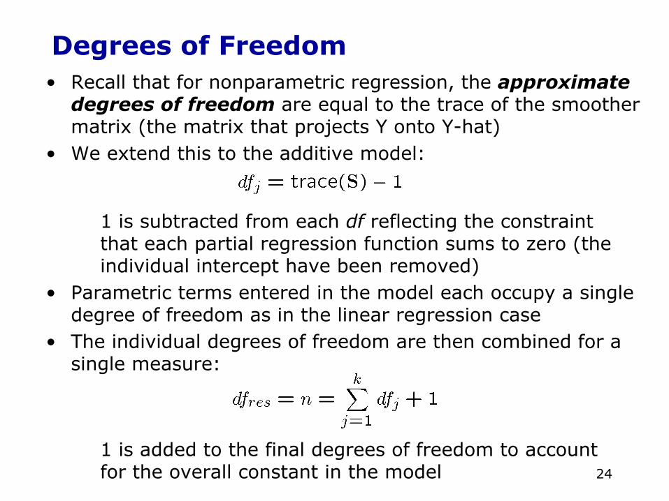
Degrees of Freedom• Recall that for nonparametric regression, the approximate

degrees of freedom are equal to the trace of the smoother matrix (the matrix that projects Y onto Y-hat)

• We extend this to the additive model:

1 is subtracted from each df reflecting the constraint that each partial regression function sums to zero (the individual intercept have been removed)

• Parametric terms entered in the model each occupy a single degree of freedom as in the linear regression case

• The individual degrees of freedom are then combined for a single measure:

1 is added to the final degrees of freedom to account for the overall constant in the model

25

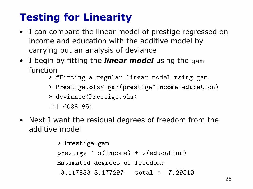
Testing for Linearity • I can compare the linear model of prestige regressed on

income and education with the additive model by carrying out an analysis of deviance

• I begin by fitting the linear model using the gamfunction

• Next I want the residual degrees of freedom from the additive model

26

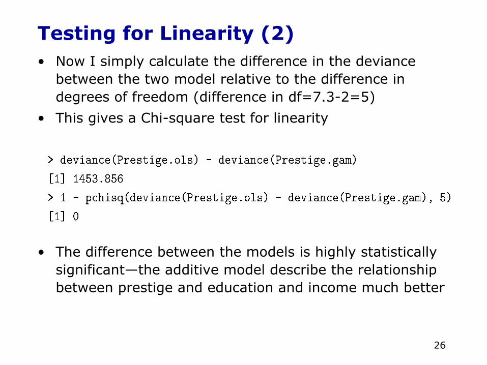
Testing for Linearity (2)• Now I simply calculate the difference in the deviance

between the two model relative to the difference in degrees of freedom (difference in df=7.3-2=5)

• This gives a Chi-square test for linearity

• The difference between the models is highly statistically significant—the additive model describe the relationship between prestige and education and income much better

27

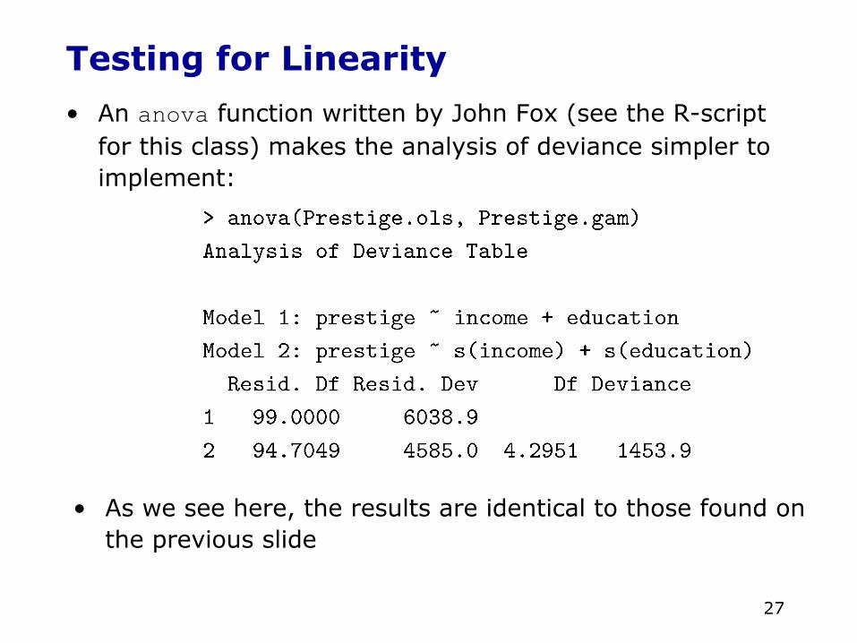
Testing for Linearity

• An anova function written by John Fox (see the R-script for this class) makes the analysis of deviance simpler to implement:

• As we see here, the results are identical to those found on the previous slide