UNIVERSITY OF CHICAGO | FINANCIAL MATHEMATICS

Regression Analysis and Quantitative Trading Strategies:

Quantitative Trading Project

Butterfly Spread Strategy

Michael BEVEN – 455613

June 3, 2016

1

STRATEGY

This project analyses the use of a butterfly spread strategy to capture returns based on volatility.

Specifically, implied volatilities of call and put options at all possible strikes are modeled for

predicting movement in the at-the-money implied volatility.

The strategy buys (sells) a call and put at-the-money with the same expiration date. A call and a put

are also sold (bought) at strikes B units above and below the at-the-money strike respectively. These

latter options are the "wings" of the butterfly. These wings offset the costs and overall exposure of

the strategy because the opposite side of the at-the-money trade is taken.

Other volatility capturing spreads exist (Hull Chapter 9 and Natenberg Chapter 8), however the

butterfly has some desirable traits. Specifically, the butterfly has no view on the direction of the

underlying (such as strips, straps, and backspreads), and risk management is incorporated into the

spread (with wing stops).

Strikes on options are not continuous, therefore "at-the-money" means to the nearest strike based

on the current underlying price. Strikes are in increments of 5 for the example used in this project.

This strategy is re-evaluated daily; closing prices of the options and the underlying are used for

calculations to decide on whether to trade at next open of the markets.

We are able to hedge the butterfly spread using delta hedging techniques, which will make a total of

five trades. Further discussion is below on choosing to implement such a hedge.

Movements in implied volatilities are modeled using an exponentially weighted moving average

(EWMA) approach. The number of days of history used in the model code is denoted as M .

Differences in the EWMA prediction and option implied volatilities of today are used to decide on

whether to buy or sell the butterfly tomorrow. Specifically, if the EWMA is greater than the implied

volatility level today by l , then we presume implied volatilities of the options will rise. Therefore we

buy the butterfly. If the EWMA is less than the implied volatility level today by k, then we presume

implied volatilities of the options will fall. Therefore we sell the butterfly. The spread position is

re-evaluated daily.

The rationale of this strategy is that prices (or volatilities) move along a path of least resistance

(Lefevre). This strategy aims to identify this path. Burghardt and Lane provide insights into how

volatility may be mispriced and how this can be exploited using volatility cones, however this report

aims to test the more flexible EWMA approach.

The maximum cost of the strategy is B (discussed further later); capital is set at 3B .

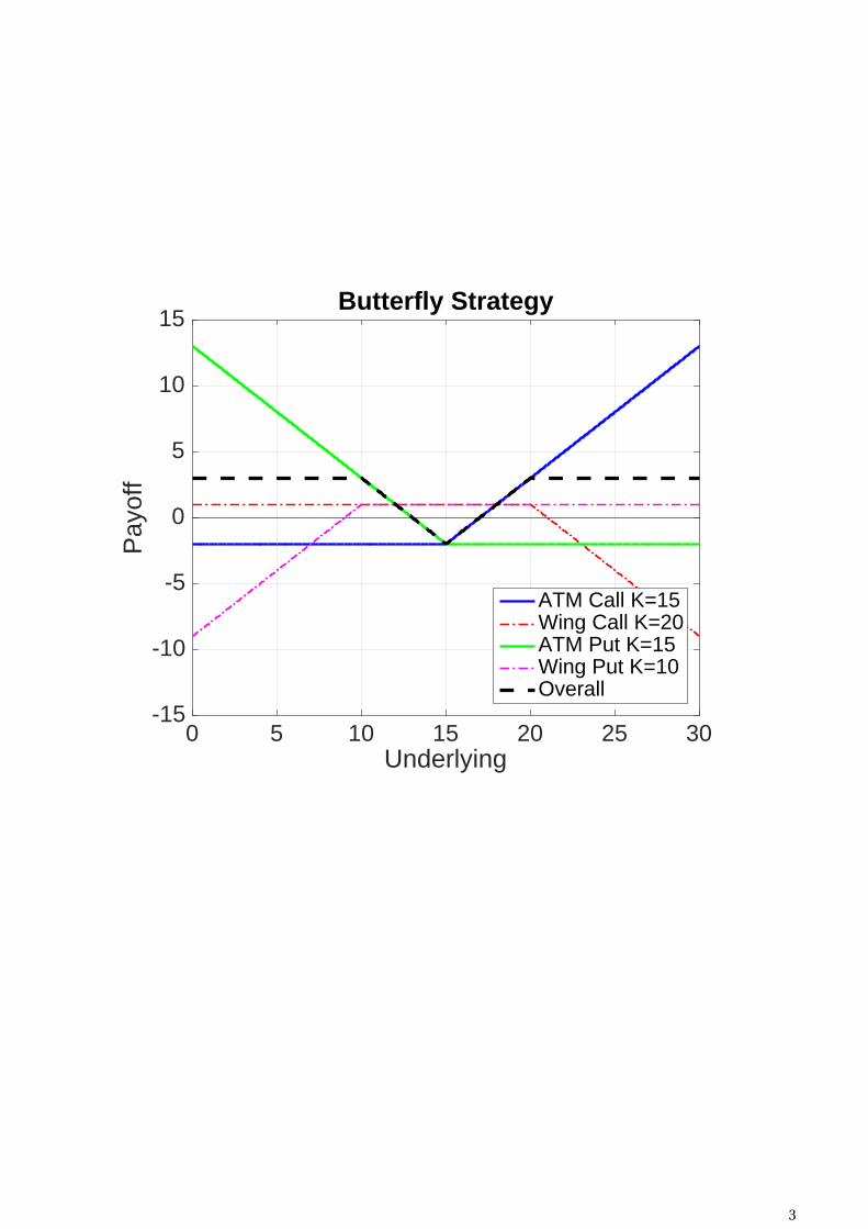
Below is an illustration of the butterfly’s payoff structure, given a long position in the spread. The

underlying must move up or down by a certain amount for the payoff to be positive.

2

0 5 10 15 20 25 30Underlying

-15

-10

-5

0

5

10

15

Pay

off

Butterfly Strategy

ATM Call K=15Wing Call K=20ATM Put K=15Wing Put K=10Overall

3

MODEL CONSTRUCTION

Here is a step-by-step walk-through of the code (written in Python) that implements the butterfly:

First the project is set up. To run this code locally, project_path must be changed:

#~*~*~*~*~*~*~*~*~*~*~*~*~*~*~*~*~*~*~*~*## Michael Hyeong-Seok Beven ## University of Chicago ## Financial Mathematics ## Quantitative Strategies and Regression ## Final Project ##~*~*~*~*~*~*~*~*~*~*~*~*~*~*~*~*~*~*~*~*#

################# python setup #################

import pandas as pdimport Quandlimport numpy as npfrom numpy import sqrt, pi, log, exp, nan, isnan, cumsum, arangefrom scipy.stats import normimport datetimeimport matplotlib.pyplot as pltimport keyring as kr # hidden passwordkey = kr.get_password(’Quandl’,’mbeven’)import osimport warningswarnings.filterwarnings(’ignore’)pd.set_option(’display.notebook_repr_html’, False)pd.set_option(’display.max_columns’, 10)pd.set_option(’display.max_rows’, 20)pd.set_option(’display.width’, 82)pd.set_option(’precision’, 6)project_path = ’/Users/michaelbeven/Documents/06_School/2016 Spring/\FINM_2016_SPRING/FINM 33150/Project’images_directory = project_path+’/Pitchbook/Images/’

Parameters are then set for the project. The expiry on the chosen underlying and options (S&P 500

E-mini June 2016 futures and options) is June 17, 2016. M(integer), l(non-negative real),

k(non-negative real), and B(increments of 5) are all adjustable.

4

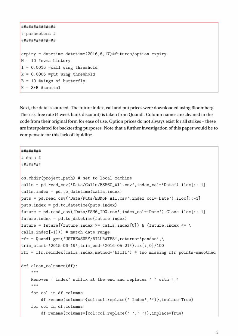
############### parameters ###############

expiry = datetime.datetime(2016,6,17)#futures/option expiryM = 10 #ewma historyl = 0.0016 #call wing thresholdk = 0.0006 #put wing thresholdB = 10 #wings of butterflyK = 3*B #capital

Next, the data is sourced. The future index, call and put prices were downloaded using Bloomberg.

The risk-free rate (4 week bank discount) is taken from Quandl. Column names are cleaned in the

code from their original form for ease of use. Option prices do not always exist for all strikes – these

are interpolated for backtesting purposes. Note that a further investigation of this paper would be to

compensate for this lack of liquidity:

######### data #########

os.chdir(project_path) # set to local machinecalls = pd.read_csv(’Data/Calls/ESM6C_All.csv’,index_col=’Date’).iloc[::-1]calls.index = pd.to_datetime(calls.index)puts = pd.read_csv(’Data/Puts/ESM6P_All.csv’,index_col=’Date’).iloc[::-1]puts.index = pd.to_datetime(puts.index)future = pd.read_csv(’Data/ESM6_IDX.csv’,index_col=’Date’).Close.iloc[::-1]future.index = pd.to_datetime(future.index)future = future[(future.index >= calls.index[0]) & (future.index <= \calls.index[-1])] # match date rangerfr = Quandl.get(’USTREASURY/BILLRATES’,returns=’pandas’,\trim_start=’2015-06-19’,trim_end=’2016-05-21’).ix[:,0]/100rfr = rfr.reindex(calls.index,method=’bfill’) # two missing rfr points-smoothed

def clean_colnames(df):"""Removes ’ Index’ suffix at the end and replaces ’ ’ with ’_’"""for col in df.columns:

df.rename(columns={col:col.replace(’ Index’,’’)},inplace=True)for col in df.columns:

df.rename(columns={col:col.replace(’ ’,’_’)},inplace=True)

5

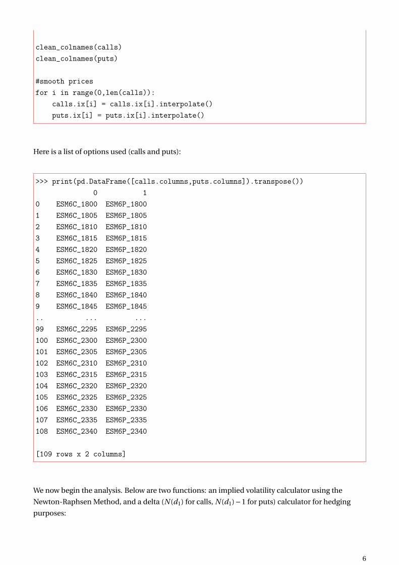
clean_colnames(calls)clean_colnames(puts)

#smooth pricesfor i in range(0,len(calls)):

calls.ix[i] = calls.ix[i].interpolate()puts.ix[i] = puts.ix[i].interpolate()

Here is a list of options used (calls and puts):

>>> print(pd.DataFrame([calls.columns,puts.columns]).transpose())0 1

0 ESM6C_1800 ESM6P_18001 ESM6C_1805 ESM6P_18052 ESM6C_1810 ESM6P_18103 ESM6C_1815 ESM6P_18154 ESM6C_1820 ESM6P_18205 ESM6C_1825 ESM6P_18256 ESM6C_1830 ESM6P_18307 ESM6C_1835 ESM6P_18358 ESM6C_1840 ESM6P_18409 ESM6C_1845 ESM6P_1845.. ... ...99 ESM6C_2295 ESM6P_2295100 ESM6C_2300 ESM6P_2300101 ESM6C_2305 ESM6P_2305102 ESM6C_2310 ESM6P_2310103 ESM6C_2315 ESM6P_2315104 ESM6C_2320 ESM6P_2320105 ESM6C_2325 ESM6P_2325106 ESM6C_2330 ESM6P_2330107 ESM6C_2335 ESM6P_2335108 ESM6C_2340 ESM6P_2340

[109 rows x 2 columns]

We now begin the analysis. Below are two functions: an implied volatility calculator using the

Newton-Raphsen Method, and a delta (N (d1) for calls, N (d1)−1 for puts) calculator for hedging

purposes:

6

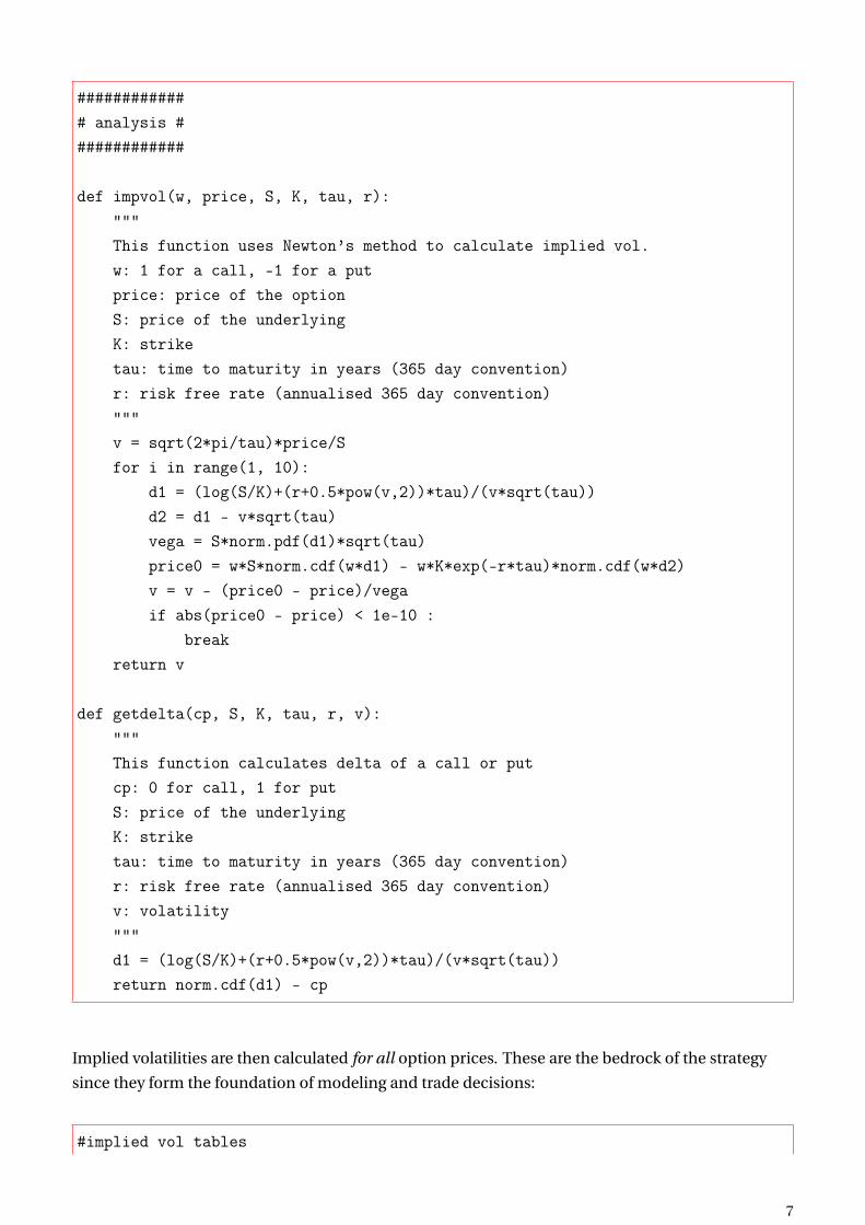
############# analysis #############

def impvol(w, price, S, K, tau, r):"""This function uses Newton’s method to calculate implied vol.w: 1 for a call, -1 for a putprice: price of the optionS: price of the underlyingK: striketau: time to maturity in years (365 day convention)r: risk free rate (annualised 365 day convention)"""v = sqrt(2*pi/tau)*price/Sfor i in range(1, 10):

d1 = (log(S/K)+(r+0.5*pow(v,2))*tau)/(v*sqrt(tau))d2 = d1 - v*sqrt(tau)vega = S*norm.pdf(d1)*sqrt(tau)price0 = w*S*norm.cdf(w*d1) - w*K*exp(-r*tau)*norm.cdf(w*d2)v = v - (price0 - price)/vegaif abs(price0 - price) < 1e-10 :

breakreturn v

def getdelta(cp, S, K, tau, r, v):"""This function calculates delta of a call or putcp: 0 for call, 1 for putS: price of the underlyingK: striketau: time to maturity in years (365 day convention)r: risk free rate (annualised 365 day convention)v: volatility"""d1 = (log(S/K)+(r+0.5*pow(v,2))*tau)/(v*sqrt(tau))return norm.cdf(d1) - cp

Implied volatilities are then calculated for all option prices. These are the bedrock of the strategy

since they form the foundation of modeling and trade decisions:

#implied vol tables

7

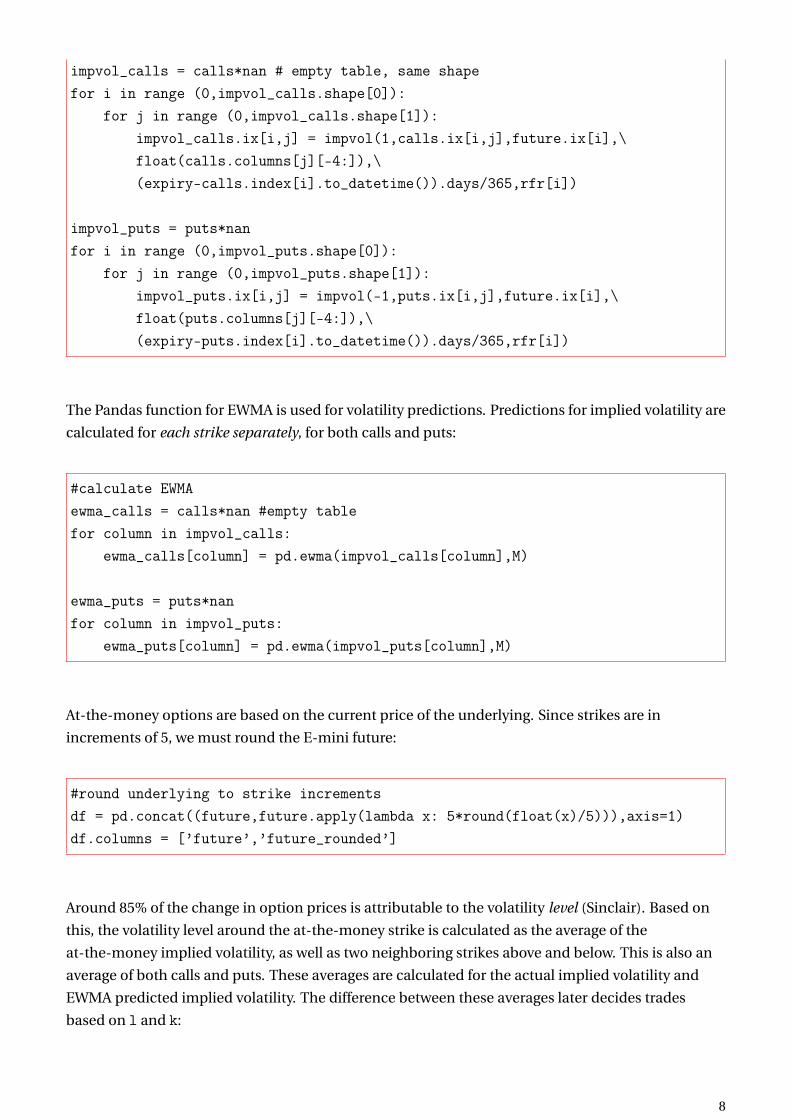
impvol_calls = calls*nan # empty table, same shapefor i in range (0,impvol_calls.shape[0]):

for j in range (0,impvol_calls.shape[1]):impvol_calls.ix[i,j] = impvol(1,calls.ix[i,j],future.ix[i],\float(calls.columns[j][-4:]),\(expiry-calls.index[i].to_datetime()).days/365,rfr[i])

impvol_puts = puts*nanfor i in range (0,impvol_puts.shape[0]):

for j in range (0,impvol_puts.shape[1]):impvol_puts.ix[i,j] = impvol(-1,puts.ix[i,j],future.ix[i],\float(puts.columns[j][-4:]),\(expiry-puts.index[i].to_datetime()).days/365,rfr[i])

The Pandas function for EWMA is used for volatility predictions. Predictions for implied volatility are

calculated for each strike separately, for both calls and puts:

#calculate EWMAewma_calls = calls*nan #empty tablefor column in impvol_calls:

ewma_calls[column] = pd.ewma(impvol_calls[column],M)

ewma_puts = puts*nanfor column in impvol_puts:

ewma_puts[column] = pd.ewma(impvol_puts[column],M)

At-the-money options are based on the current price of the underlying. Since strikes are in

increments of 5, we must round the E-mini future:

#round underlying to strike incrementsdf = pd.concat((future,future.apply(lambda x: 5*round(float(x)/5))),axis=1)df.columns = [’future’,’future_rounded’]

Around 85% of the change in option prices is attributable to the volatility level (Sinclair). Based on

this, the volatility level around the at-the-money strike is calculated as the average of the

at-the-money implied volatility, as well as two neighboring strikes above and below. This is also an

average of both calls and puts. These averages are calculated for the actual implied volatility and

EWMA predicted implied volatility. The difference between these averages later decides trades

based on l and k:

8

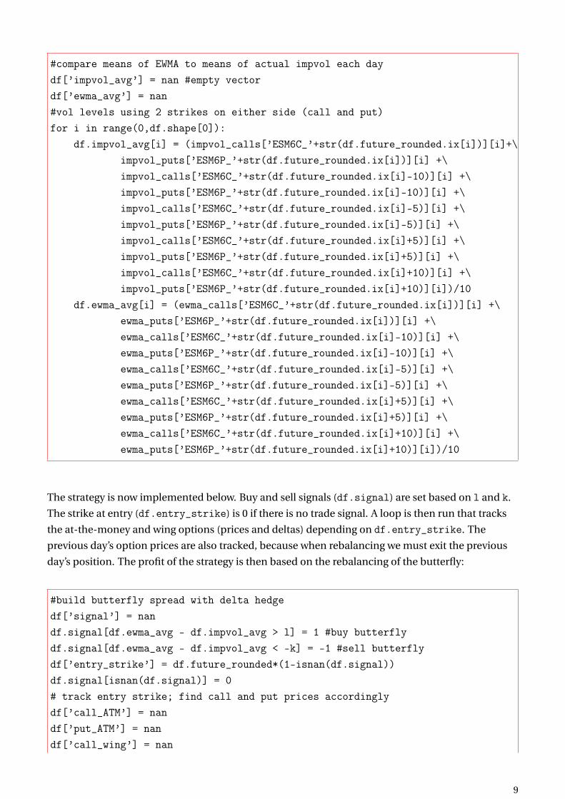
#compare means of EWMA to means of actual impvol each daydf[’impvol_avg’] = nan #empty vectordf[’ewma_avg’] = nan#vol levels using 2 strikes on either side (call and put)for i in range(0,df.shape[0]):

df.impvol_avg[i] = (impvol_calls[’ESM6C_’+str(df.future_rounded.ix[i])][i]+\impvol_puts[’ESM6P_’+str(df.future_rounded.ix[i])][i] +\impvol_calls[’ESM6C_’+str(df.future_rounded.ix[i]-10)][i] +\impvol_puts[’ESM6P_’+str(df.future_rounded.ix[i]-10)][i] +\impvol_calls[’ESM6C_’+str(df.future_rounded.ix[i]-5)][i] +\impvol_puts[’ESM6P_’+str(df.future_rounded.ix[i]-5)][i] +\impvol_calls[’ESM6C_’+str(df.future_rounded.ix[i]+5)][i] +\impvol_puts[’ESM6P_’+str(df.future_rounded.ix[i]+5)][i] +\impvol_calls[’ESM6C_’+str(df.future_rounded.ix[i]+10)][i] +\impvol_puts[’ESM6P_’+str(df.future_rounded.ix[i]+10)][i])/10

df.ewma_avg[i] = (ewma_calls[’ESM6C_’+str(df.future_rounded.ix[i])][i] +\ewma_puts[’ESM6P_’+str(df.future_rounded.ix[i])][i] +\ewma_calls[’ESM6C_’+str(df.future_rounded.ix[i]-10)][i] +\ewma_puts[’ESM6P_’+str(df.future_rounded.ix[i]-10)][i] +\ewma_calls[’ESM6C_’+str(df.future_rounded.ix[i]-5)][i] +\ewma_puts[’ESM6P_’+str(df.future_rounded.ix[i]-5)][i] +\ewma_calls[’ESM6C_’+str(df.future_rounded.ix[i]+5)][i] +\ewma_puts[’ESM6P_’+str(df.future_rounded.ix[i]+5)][i] +\ewma_calls[’ESM6C_’+str(df.future_rounded.ix[i]+10)][i] +\ewma_puts[’ESM6P_’+str(df.future_rounded.ix[i]+10)][i])/10

The strategy is now implemented below. Buy and sell signals (df.signal) are set based on l and k.

The strike at entry (df.entry_strike) is 0 if there is no trade signal. A loop is then run that tracks

the at-the-money and wing options (prices and deltas) depending on df.entry_strike. The

previous day’s option prices are also tracked, because when rebalancing we must exit the previous

day’s position. The profit of the strategy is then based on the rebalancing of the butterfly:

#build butterfly spread with delta hedgedf[’signal’] = nandf.signal[df.ewma_avg - df.impvol_avg > l] = 1 #buy butterflydf.signal[df.ewma_avg - df.impvol_avg < -k] = -1 #sell butterflydf[’entry_strike’] = df.future_rounded*(1-isnan(df.signal))df.signal[isnan(df.signal)] = 0# track entry strike; find call and put prices accordinglydf[’call_ATM’] = nandf[’put_ATM’] = nandf[’call_wing’] = nan

9

df[’put_wing’] = nandf[’call_ATM_delta’] = nandf[’put_ATM_delta’] = nandf[’call_wing_delta’] = nandf[’put_wing_delta’] = nanfor i in range(1,len(df)):

if df.signal[i] == 0:df.call_ATM[i] = 0df.put_ATM[i] = 0df.call_wing[i] = 0df.put_wing[i] = 0df.call_ATM_delta[i] = 0df.put_ATM_delta[i] = 0df.call_wing_delta[i] = 0df.put_wing_delta[i] = 0

else:df.call_ATM[i] = calls.ix[i][’ESM6C_’+str(df.entry_strike[i])]df.call_ATM_delta[i] = getdelta(0, df.future[i], df.entry_strike[i],\(expiry-df.index[i].to_datetime()).days/365,rfr[i], \impvol_calls.ix[i][’ESM6C_’+str(df.entry_strike[i])])df.put_ATM[i] = puts.ix[i][’ESM6P_’+str(df.entry_strike[i])]df.put_ATM_delta[i] = getdelta(1, df.future[i], df.entry_strike[i],\(expiry-df.index[i].to_datetime()).days/365,rfr[i], \impvol_puts.ix[i][’ESM6P_’+str(df.entry_strike[i])])df.call_wing[i] = calls.ix[i][’ESM6C_’+str(df.entry_strike[i]+B)]df.call_wing_delta[i] = getdelta(0, df.future[i], df.entry_strike[i]+B,\(expiry-df.index[i].to_datetime()).days/365,rfr[i],\impvol_calls.ix[i][’ESM6C_’+str(df.entry_strike[i]+10)])df.put_wing[i] = puts.ix[i][’ESM6P_’+str(df.entry_strike[i]-B)]df.put_wing_delta[i] = getdelta(1, df.future[i], df.entry_strike[i]+B,\(expiry-df.index[i].to_datetime()).days/365,rfr[i],\impvol_puts.ix[i][’ESM6P_’+str(df.entry_strike[i]-10)])

df[’delta_hedge’] = df.call_ATM_delta + df.put_ATM_delta - (df.call_wing_delta\+ df.put_wing_delta)

# track previous day’s position valuedf[’call_ATM_old’] = nandf[’put_ATM_old’] = nandf[’call_wing_old’] = nandf[’put_wing_old’] = nanfor i in range(1,len(df)):

if df.signal[i-1] == 0:df.call_ATM_old[i] = 0df.put_ATM_old[i] = 0df.call_wing_old[i] = 0

10

df.put_wing_old[i] = 0else:

df.call_ATM_old[i] = calls.ix[i][’ESM6C_’+str(df.entry_strike[i-1])]df.put_ATM_old[i] = puts.ix[i][’ESM6P_’+str(df.entry_strike[i-1])]df.call_wing_old[i] = calls.ix[i][’ESM6C_’+str(df.entry_strike[i-1]+B)]df.put_wing_old[i] = puts.ix[i][’ESM6P_’+str(df.entry_strike[i-1]-B)]

df = df[2:]df[’butterfly’] = df.signal*((df.call_wing + df.put_wing) - \(df.call_ATM + df.put_ATM))df[’butterfly_old’] = df.shift(1).signal*((df.call_wing_old + \df.put_wing_old) - (df.call_ATM_old + df.put_ATM_old))df[’profit’] = df.shift(1).butterfly - df.butterfly_olddf.profit[0] = df.signal[0]*((df.call_wing[0] + df.put_wing[0]) - \(df.call_ATM[0] + df.put_ATM[0]))df[’cum_profit’] = cumsum(df.profit)

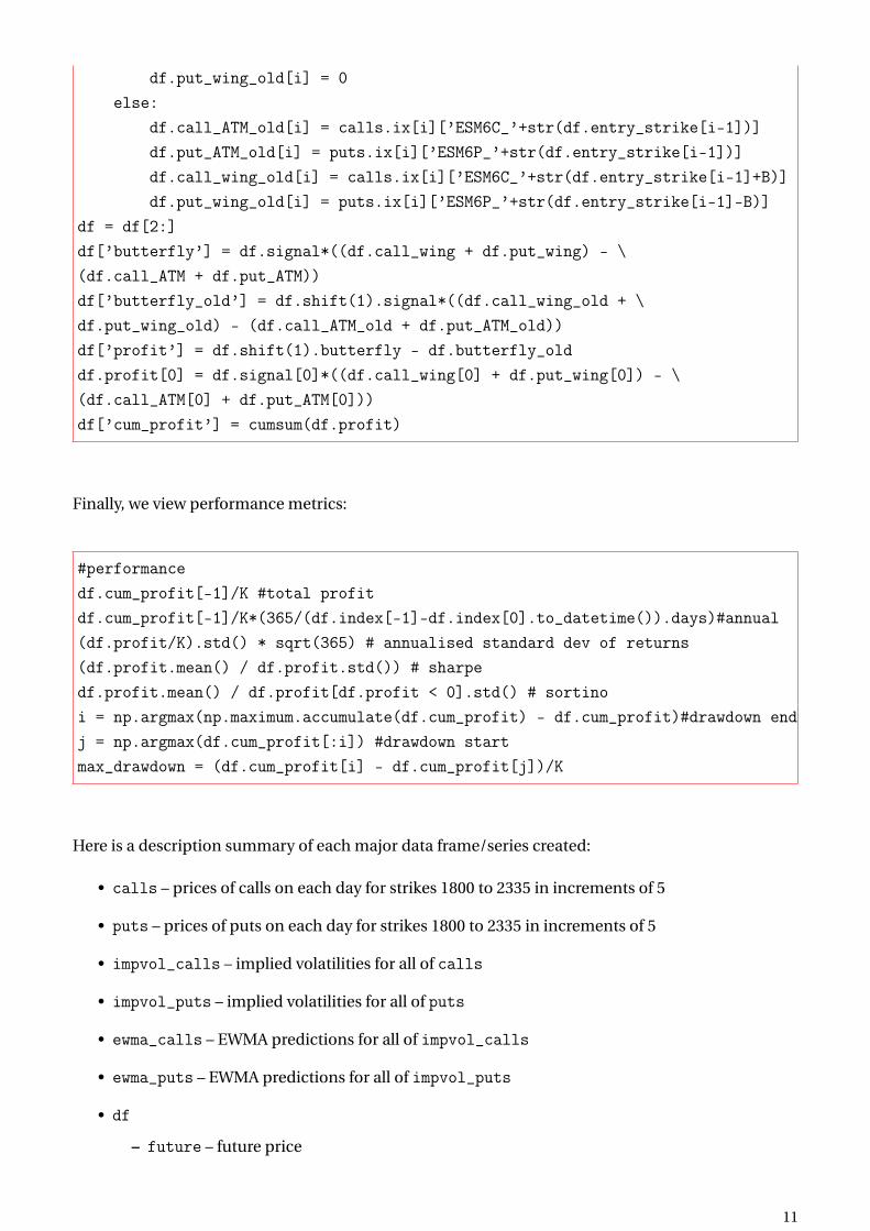
Finally, we view performance metrics:

#performancedf.cum_profit[-1]/K #total profitdf.cum_profit[-1]/K*(365/(df.index[-1]-df.index[0].to_datetime()).days)#annual(df.profit/K).std() * sqrt(365) # annualised standard dev of returns(df.profit.mean() / df.profit.std()) # sharpedf.profit.mean() / df.profit[df.profit < 0].std() # sortinoi = np.argmax(np.maximum.accumulate(df.cum_profit) - df.cum_profit)#drawdown endj = np.argmax(df.cum_profit[:i]) #drawdown startmax_drawdown = (df.cum_profit[i] - df.cum_profit[j])/K

Here is a description summary of each major data frame/series created:

• calls – prices of calls on each day for strikes 1800 to 2335 in increments of 5

• puts – prices of puts on each day for strikes 1800 to 2335 in increments of 5

• impvol_calls – implied volatilities for all of calls

• impvol_puts – implied volatilities for all of puts

• ewma_calls – EWMA predictions for all of impvol_calls

• ewma_puts – EWMA predictions for all of impvol_puts

• df

– future – future price

11

– future_rounded – future rounded to nearest 5

– impvol_avg – average implied volatility (as described above)

– ewma_avg – average ewma volatility (as described above)

– signal – buy/sell signal

– entry_strike – strike at entry of trade

– call_ATM – at-the-money call price at entry of trade

– put_ATM – at-the-money put price at entry of trade

– call_wing – wing call price at entry of trade

– put_wing – wing put price at entry of trade

– call_ATM_delta – at-the-money call delta at entry of trade

– put_ATM_delta – at-the-money put delta at entry of trade

– call_wing_delta – wing call delta at entry of trade

– put_wing_delta – wing put delta at entry of trade

– delta_hedge – sum of deltas

– call_ATM_old – previous day’s current at-the-money call price

– put_ATM_old – previous day’s current at-the-money put price

– call_wing_old – previous day’s current wing call price

– put_wing_old – previous day’s current wing put price

– butterfly – total value for the spread

– butterfly_old – total updated value for the spread from previous day

– profit – difference in today’s spread value and yesterday’s spread value

– cum_profit – cumulative profit

INVESTMENT UNIVERSE

The butterfly spread strategy is adaptable to many underlying assets and respective options, such as:

commodities, equities, indexes, foreign exchange, fixed income and so on. The strategy requires that

options in particular are liquid. This is essential for properly building the butterfly, with two options

at-the-money and two at the wings. These options in the wings act as stops; they stop potential

profits in a long butterfly and stop potential losses in a short butterfly. These wings ultimately limit

the investment capital required for the strategy, expanding the investment universe to more

expensive products.

This strategy can also employ a delta hedge, however one must be careful in using this hedge. The

hedge removes risk captured by directional exposure in the options versus the underlying, however

this risk is very small given the symmetry of the butterfly. The dominant risk in this strategy is thus

based on volatility (which we clearly do not want to hedge).

The strategy also easily adapts to shorter investment horizons, such as intraday.

12

COMPETITIVE EDGE

The EWMA approach for measuring what implied volatility is versus what it ought to be is flexible

and easily adjusted (changing historical days). This strategy is also mechanically different from

many positions in investment portfolios (e.g. value or growth stocks based portfolios) since the

trade driver is option implied volatilities. Therefore, this strategy may add alpha to portfolios. A

diversified portfolio of butterfly spreads could also be created. As previously mentioned, the

butterfly also has a low cost structure. Another great feature of this spread is based in its symmetry; a

view on market direction is not required.

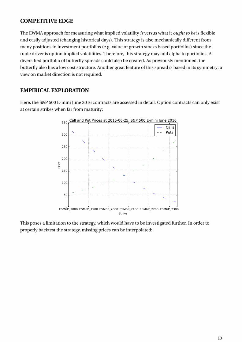
EMPIRICAL EXPLORATION

Here, the S&P 500 E-mini June 2016 contracts are assessed in detail. Option contracts can only exist

at certain strikes when far from maturity:

ESM6P_1800 ESM6P_1900 ESM6P_2000 ESM6P_2100 ESM6P_2200 ESM6P_2300Strike

0

50

100

150

200

250

300

350

Pri

ce

Call and Put Prices at 2015-06-25, S&P 500 E-mini June 2016

CallsPuts

This poses a limitation to the strategy, which would have to be investigated further. In order to

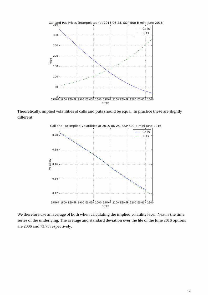
properly backtest the strategy, missing prices can be interpolated:

13

ESM6P_1800 ESM6P_1900 ESM6P_2000 ESM6P_2100 ESM6P_2200 ESM6P_2300Strike

0

50

100

150

200

250

300

350

Pri

ce

Call and Put Prices (Interpolated) at 2015-06-25, S&P 500 E-mini June 2016

CallsPuts

Theoretically, implied volatilities of calls and puts should be equal. In practice these are slightly

different:

ESM6P_1800 ESM6P_1900 ESM6P_2000 ESM6P_2100 ESM6P_2200 ESM6P_2300Strike

0.12

0.14

0.16

0.18

0.20

Vola

tilit

y

Call and Put Implied Volatilities at 2015-06-25, S&P 500 E-mini June 2016

CallsPuts

We therefore use an average of both when calculating the implied volatility level. Next is the time

series of the underlying. The average and standard deviation over the life of the June 2016 options

are 2006 and 73.75 respectively:

14

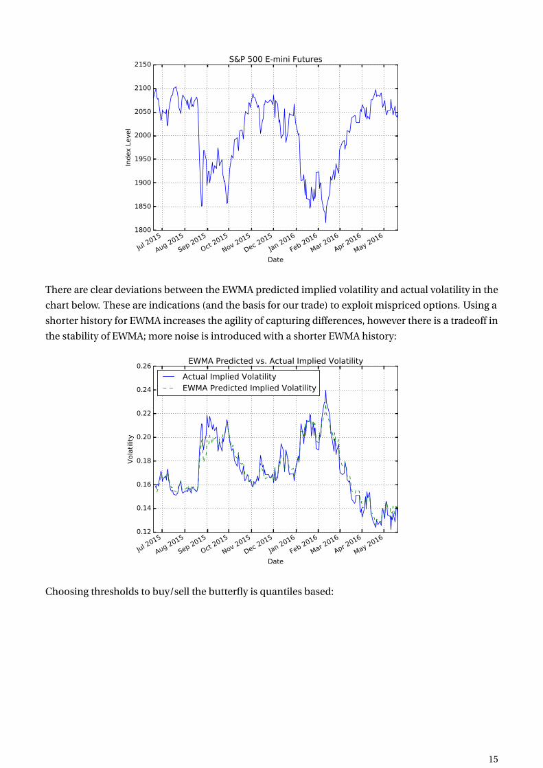
Jul 2015

Aug 2015

Sep 2015

Oct 2015

Nov 2015

Dec 2015

Jan 2016

Feb 2016

Mar 2016

Apr 2016

May 2016

Date

1800

1850

1900

1950

2000

2050

2100

2150

Index L

evel

S&P 500 E-mini Futures

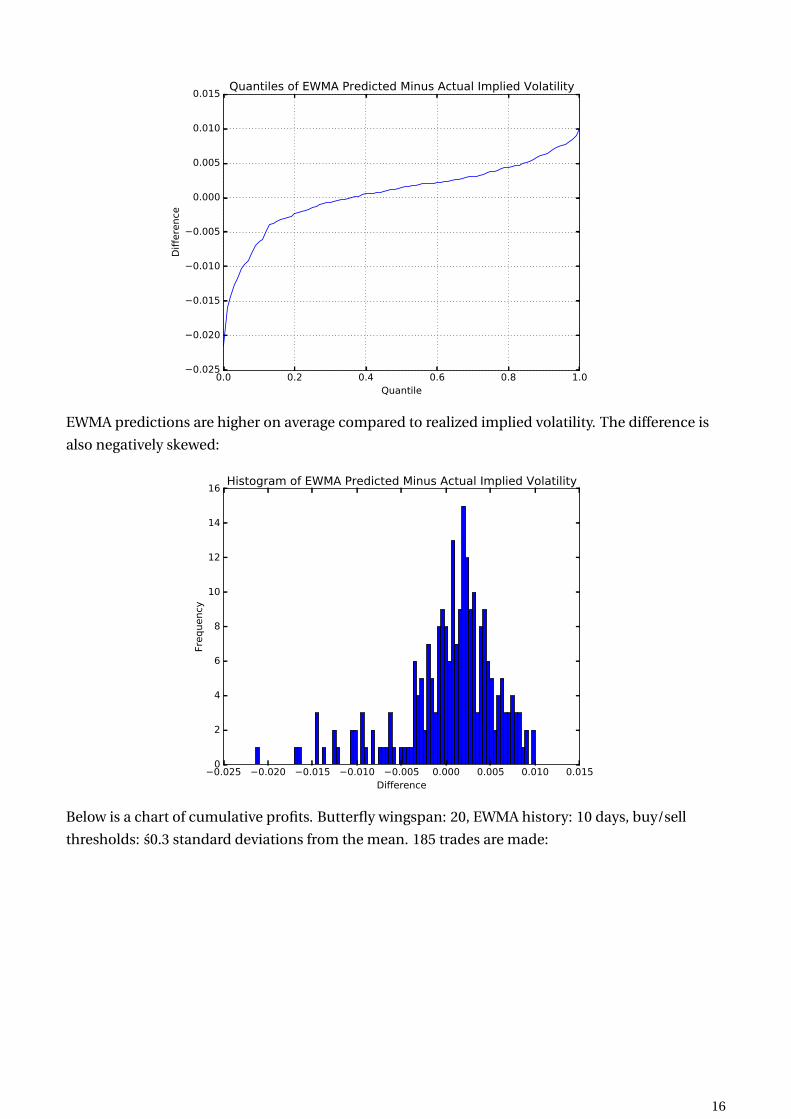
There are clear deviations between the EWMA predicted implied volatility and actual volatility in the

chart below. These are indications (and the basis for our trade) to exploit mispriced options. Using a

shorter history for EWMA increases the agility of capturing differences, however there is a tradeoff in

the stability of EWMA; more noise is introduced with a shorter EWMA history:

Jul 2015

Aug 2015

Sep 2015

Oct 2015

Nov 2015

Dec 2015

Jan 2016

Feb 2016

Mar 2016

Apr 2016

May 2016

Date

0.12

0.14

0.16

0.18

0.20

0.22

0.24

0.26

Vola

tilit

y

EWMA Predicted vs. Actual Implied Volatility

Actual Implied VolatilityEWMA Predicted Implied Volatility

Choosing thresholds to buy/sell the butterfly is quantiles based:

15

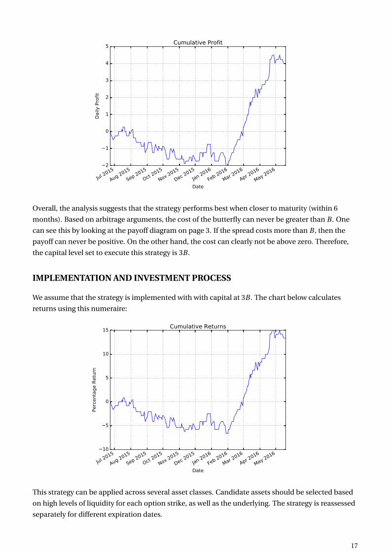
0.0 0.2 0.4 0.6 0.8 1.0Quantile

0.025

0.020

0.015

0.010

0.005

0.000

0.005

0.010

0.015

Diffe

rence

Quantiles of EWMA Predicted Minus Actual Implied Volatility

EWMA predictions are higher on average compared to realized implied volatility. The difference is

also negatively skewed:

0.025 0.020 0.015 0.010 0.005 0.000 0.005 0.010 0.015Difference

0

2

4

6

8

10

12

14

16

Frequency

Histogram of EWMA Predicted Minus Actual Implied Volatility

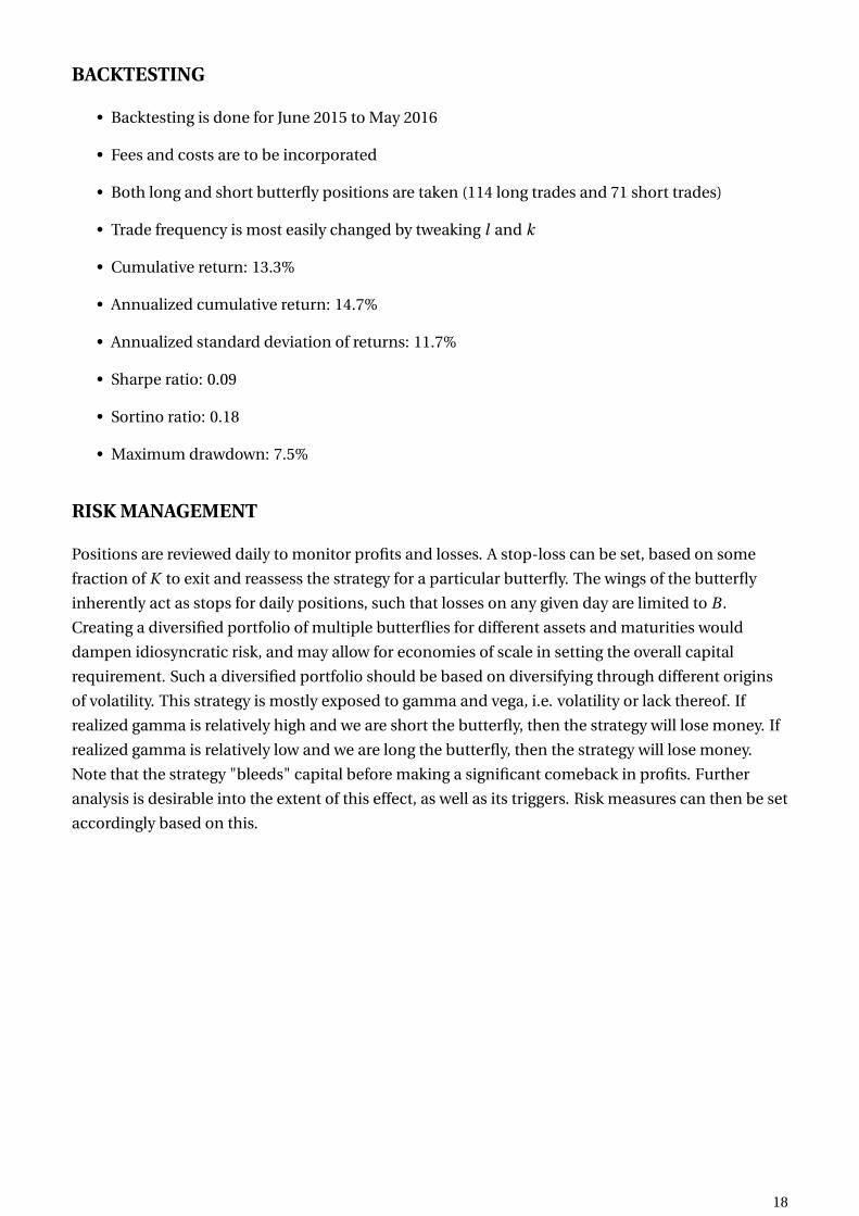
Below is a chart of cumulative profits. Butterfly wingspan: 20, EWMA history: 10 days, buy/sell

thresholds: s0.3 standard deviations from the mean. 185 trades are made:

16

Jul 2015

Aug 2015

Sep 2015

Oct 2015

Nov 2015

Dec 2015

Jan 2016

Feb 2016

Mar 2016

Apr 2016

May 2016

Date

2

1

0

1

2

3

4

5

Daily

Pro

fit

Cumulative Profit

Overall, the analysis suggests that the strategy performs best when closer to maturity (within 6

months). Based on arbitrage arguments, the cost of the butterfly can never be greater than B . One

can see this by looking at the payoff diagram on page 3. If the spread costs more than B , then the

payoff can never be positive. On the other hand, the cost can clearly not be above zero. Therefore,

the capital level set to execute this strategy is 3B .

IMPLEMENTATION AND INVESTMENT PROCESS

We assume that the strategy is implemented with with capital at 3B . The chart below calculates

returns using this numeraire:

Jul 2015

Aug 2015

Sep 2015

Oct 2015

Nov 2015

Dec 2015

Jan 2016

Feb 2016

Mar 2016

Apr 2016

May 2016

Date

10

5

0

5

10

15

Perc

enta

ge R

etu

rn

Cumulative Returns

This strategy can be applied across several asset classes. Candidate assets should be selected based

on high levels of liquidity for each option strike, as well as the underlying. The strategy is reassessed

separately for different expiration dates.

17

BACKTESTING

• Backtesting is done for June 2015 to May 2016

• Fees and costs are to be incorporated

• Both long and short butterfly positions are taken (114 long trades and 71 short trades)

• Trade frequency is most easily changed by tweaking l and k

• Cumulative return: 13.3%

• Annualized cumulative return: 14.7%

• Annualized standard deviation of returns: 11.7%

• Sharpe ratio: 0.09

• Sortino ratio: 0.18

• Maximum drawdown: 7.5%

RISK MANAGEMENT

Positions are reviewed daily to monitor profits and losses. A stop-loss can be set, based on some

fraction of K to exit and reassess the strategy for a particular butterfly. The wings of the butterfly

inherently act as stops for daily positions, such that losses on any given day are limited to B .

Creating a diversified portfolio of multiple butterflies for different assets and maturities would

dampen idiosyncratic risk, and may allow for economies of scale in setting the overall capital

requirement. Such a diversified portfolio should be based on diversifying through different origins

of volatility. This strategy is mostly exposed to gamma and vega, i.e. volatility or lack thereof. If

realized gamma is relatively high and we are short the butterfly, then the strategy will lose money. If

realized gamma is relatively low and we are long the butterfly, then the strategy will lose money.

Note that the strategy "bleeds" capital before making a significant comeback in profits. Further

analysis is desirable into the extent of this effect, as well as its triggers. Risk measures can then be set

accordingly based on this.

18

ABOUT THE MANAGER

MICHAEL BEVEN graduated as a National Merit Scholar from the Australian National University in

2012 with a Bachelor of Actuarial Studies and a Bachelor of Finance (Majors in Quantitative and

Corporate Finance). He is currently completing a Master of Science in Financial Mathematics at the

University of Chicago. Prior to starting at the University of Chicago, Michael was an Actuarial

Analyst in Sydney at Quantium, a data analytics focused actuarial consultancy. He has also interned

at Macquarie Group and Westpac Institutional Bank in quantitative risk analytics. Michael is deeply

interested in electronic trading and sees Chicago as a great place to progress his career.

19

REFERENCES

Burghardt, Galen and Lane, Morton. "How to Tell If Options Are Cheap." Journal of Portfolio

Management, 1990, 16(2), pp. 72-78.

Hull, John. Fundamentals Of Futures And Options Markets. Upper Saddle River, NJ: Pearson

Prentice Hall, 2008. Print.

Lefevre, Edwin. Reminiscences of a Stock Operator. Hoboken, NJ: Wiley, 2010.

Sinclair, Euan. Volatility Trading. Hoboken, NJ: Wiley, 2008.

Natenberg, Sheldon. Option Volatility & Pricing: Advanced Trading Strategies and Techniques.

Chicago, IL: Probus, 1994.

20