Registration of multiple ToF camera point clouds327071/FULLTEXT01.pdf · Registration of multiple ToF camera point clouds Tobias Hedlund ... Chetverikov et al. (2005) proposed a version

Registration of multiple ToF camerapoint clouds

Tobias Hedlund

June 23, 2010Master’s Thesis in Engineering Physics, 30 ECTS-credits

Supervisor at CS-UmU: Niclas BorlinSupervisors at Adopticum: Jonas Sjoberg & Emil Hallstig

Examiner: Christina Igasto

UMEA UNIVERSITYDEPARTMENT OF PHYSICS

SE-901 87 UMEASWEDEN

Abstract

Buildings, maps and objects et cetera, can be modeled using a computer or reconstructed in 3D bydata from different kinds of cameras or laser scanners. This thesis concerns the latter. The recentimprovements of Time-of-Flight cameras have brought a number of new interesting research areasto the surface. Registration of several ToF camera point clouds is such an area.

A literature study has been made to summarize the research done in the area over the last twodecades. The most popular method for registering point clouds, namely the Iterative Closest Point(ICP), has been studied. In addition to this, an error relaxation algorithm was implemented to mini-mize the accumulated error of the sequential pairwise ICP.

A few different real-world test scenarios and one scenario with synthetic data were constructed.These data sets were registered with varying outcome. The obtained camera poses from the sequen-tial ICP were improved by loop closing and error relaxation.

The results illustrate the importance of having good initial guesses on the relative transformationsto obtain a correct model. Furthermore the strengths and weaknesses of the sequential ICP and theutilized error relaxation method are shown.

ii

ii

Acknowledgements

I would like to thank a number of people for supporting me in this thesis work. First of all, I wouldlike to thank Niclas Borlin who introduced me to the area of photogrammetry and image analysisa few years back. Without his enthusiasm and support as main supervisor, this wouldn’t have beenpossible.

I would also like to thank my contacts at Adopticum, Jonas Sjoberg and Emil Hallstig, for theirsupport and for making me feel at home in the company office.

Thanks to my examiner, Christina Igasto, for helping me with the report and for answering myLATEX questions.

Finally, thanks to Maria for listening to all my complaints and worries these last four and a halfmonths.

iii

iv

iv

Contents

1 Introduction 11.1 Background . . . . . . . . . . . . . . . . . . . . . . . . . . . . . . . . . . . . . . 1

1.2 Aims . . . . . . . . . . . . . . . . . . . . . . . . . . . . . . . . . . . . . . . . . . 2

1.3 Related Work . . . . . . . . . . . . . . . . . . . . . . . . . . . . . . . . . . . . . 2

2 Theory 52.1 The Pinhole Camera Model . . . . . . . . . . . . . . . . . . . . . . . . . . . . . . 5

2.2 ToF cameras . . . . . . . . . . . . . . . . . . . . . . . . . . . . . . . . . . . . . . 6

2.3 Rigid body transformations . . . . . . . . . . . . . . . . . . . . . . . . . . . . . . 7

2.4 Quaternions . . . . . . . . . . . . . . . . . . . . . . . . . . . . . . . . . . . . . . 7

2.5 Methods for estimating transformations . . . . . . . . . . . . . . . . . . . . . . . 8

2.5.1 SIFT . . . . . . . . . . . . . . . . . . . . . . . . . . . . . . . . . . . . . 9

2.5.2 RANSAC . . . . . . . . . . . . . . . . . . . . . . . . . . . . . . . . . . . 9

2.6 Calibration . . . . . . . . . . . . . . . . . . . . . . . . . . . . . . . . . . . . . . 9

2.7 ToF camera errors . . . . . . . . . . . . . . . . . . . . . . . . . . . . . . . . . . . 10

2.8 Filtering . . . . . . . . . . . . . . . . . . . . . . . . . . . . . . . . . . . . . . . . 11

2.9 ICP . . . . . . . . . . . . . . . . . . . . . . . . . . . . . . . . . . . . . . . . . . 13

2.9.1 Estimating rigid body transformations (The Procrustes Problem) . . . . . . 13

2.9.2 Selection of points . . . . . . . . . . . . . . . . . . . . . . . . . . . . . . 13

2.9.3 How to match points . . . . . . . . . . . . . . . . . . . . . . . . . . . . . 14

2.9.4 Rejection of point pairs . . . . . . . . . . . . . . . . . . . . . . . . . . . . 14

2.9.5 kd-trees . . . . . . . . . . . . . . . . . . . . . . . . . . . . . . . . . . . . 15

2.10 Loop closing and error relaxation . . . . . . . . . . . . . . . . . . . . . . . . . . . 15

3 Implementation 193.1 Preprocessing . . . . . . . . . . . . . . . . . . . . . . . . . . . . . . . . . . . . . 19

3.2 Pairwise ICP . . . . . . . . . . . . . . . . . . . . . . . . . . . . . . . . . . . . . 21

3.3 Multi-view registration . . . . . . . . . . . . . . . . . . . . . . . . . . . . . . . . 22

3.4 Loop closing . . . . . . . . . . . . . . . . . . . . . . . . . . . . . . . . . . . . . 22

3.5 Global optimization . . . . . . . . . . . . . . . . . . . . . . . . . . . . . . . . . . 23

v

vi CONTENTS

4 Experiments 254.1 Test cases . . . . . . . . . . . . . . . . . . . . . . . . . . . . . . . . . . . . . . . 25

4.1.1 Translation of the camera . . . . . . . . . . . . . . . . . . . . . . . . . . . 264.1.2 Room with reference objects . . . . . . . . . . . . . . . . . . . . . . . . . 264.1.3 Empty room . . . . . . . . . . . . . . . . . . . . . . . . . . . . . . . . . 274.1.4 The torso . . . . . . . . . . . . . . . . . . . . . . . . . . . . . . . . . . . 274.1.5 The box . . . . . . . . . . . . . . . . . . . . . . . . . . . . . . . . . . . . 284.1.6 The synthetic data . . . . . . . . . . . . . . . . . . . . . . . . . . . . . . 28

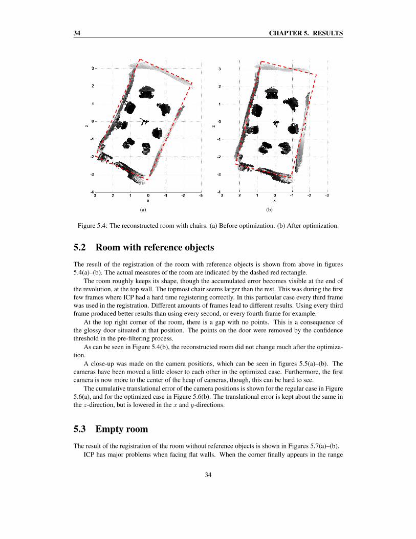
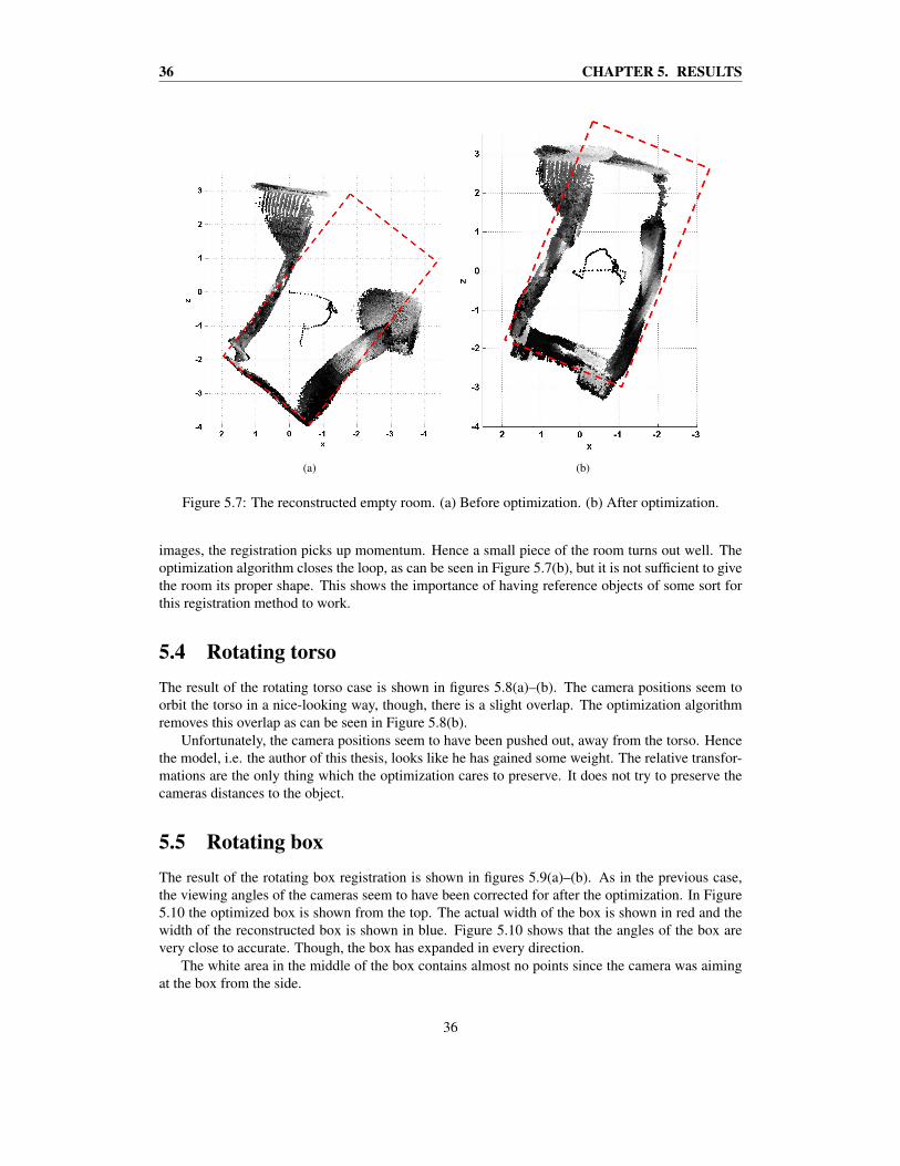
5 Results 315.1 Translation of the camera . . . . . . . . . . . . . . . . . . . . . . . . . . . . . . . 315.2 Room with reference objects . . . . . . . . . . . . . . . . . . . . . . . . . . . . . 345.3 Empty room . . . . . . . . . . . . . . . . . . . . . . . . . . . . . . . . . . . . . . 345.4 Rotating torso . . . . . . . . . . . . . . . . . . . . . . . . . . . . . . . . . . . . . 365.5 Rotating box . . . . . . . . . . . . . . . . . . . . . . . . . . . . . . . . . . . . . . 365.6 The synthetic data . . . . . . . . . . . . . . . . . . . . . . . . . . . . . . . . . . . 38

6 Discussion 43

7 Conclusions 45

8 Future work 47

References 49

vi

List of Figures

2.1 The pinhole camera model. The camera center, C, the principal point, p, and thefocal length, f . . . . . . . . . . . . . . . . . . . . . . . . . . . . . . . . . . . . . 5

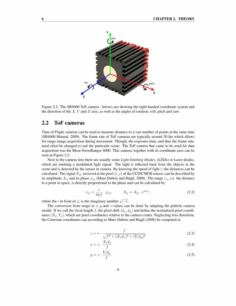
2.2 The SR4000 ToF camera. Arrows are showing the right-handed coordinate systemand the direction of the X,Y and Z-axis, as well as the angles of rotation; roll, pitchand yaw. . . . . . . . . . . . . . . . . . . . . . . . . . . . . . . . . . . . . . . . . 6

2.3 Schematic illustration of the quaternion angle representation. . . . . . . . . . . . . 82.4 Matched SIFT keypoints between two amplitude images of a ToF camera. . . . . . 92.5 Point fitting to a plane with RANSAC. Inliers, i.e. accepted points, marked by green

dots. Points further away than the distance treshold, t, marked by red dots. . . . . . 102.6 Two common artifacts of ToF cameras. . . . . . . . . . . . . . . . . . . . . . . . . 112.7 Neighborhood angle filter proposed by May et al. (2009). Two neighboring pixels

on a sensor marked in blue, pi and pi,n are points in space. . . . . . . . . . . . . . 122.8 ICP alignment of a dataset onto a model. Dataset position before registration, blue

dots. Dataset position after registration, red dots. . . . . . . . . . . . . . . . . . . 142.9 Methods for matching points. . . . . . . . . . . . . . . . . . . . . . . . . . . . . . 152.10 Graph edges between views, i.e. cameras, which are close enough. . . . . . . . . . 16

3.1 Model used to illustrate filtering techniques. . . . . . . . . . . . . . . . . . . . . . 193.2 Different filtering techniques . . . . . . . . . . . . . . . . . . . . . . . . . . . . . 203.3 The point-to-point method for determining corresponding points between datasets. 223.4 Illustration of the loop detecting algorithm. The large camera has just been added.

The cameras within the wireframe sphere fulfill the distance criterion. The camerassurrounded by a green circle also have a similar viewing direction, and thus they arematchable. Crossed over cameras are too close behind to form a loop. . . . . . . . 23

4.1 Translation of the camera . . . . . . . . . . . . . . . . . . . . . . . . . . . . . . . 264.2 The room in which the rotation scenario was done. Chairs are placed evenly spaced

as reference objects. . . . . . . . . . . . . . . . . . . . . . . . . . . . . . . . . . . 274.3 Three amplitude images from the case of the rotating torso. . . . . . . . . . . . . . 274.4 The box on a stand. . . . . . . . . . . . . . . . . . . . . . . . . . . . . . . . . . . 284.5 The synthetic data constructed with Matlab’s peaks-function. . . . . . . . . . . . 29

vii

viii LIST OF FIGURES

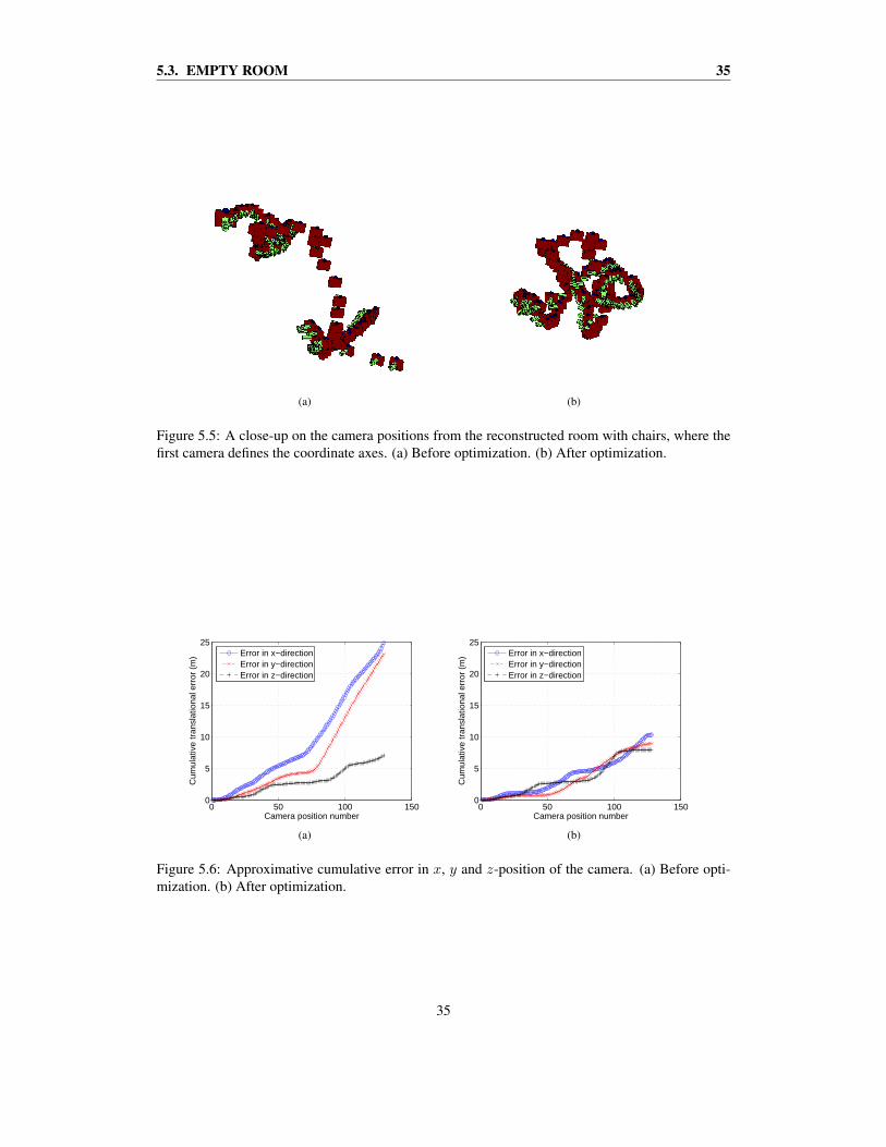
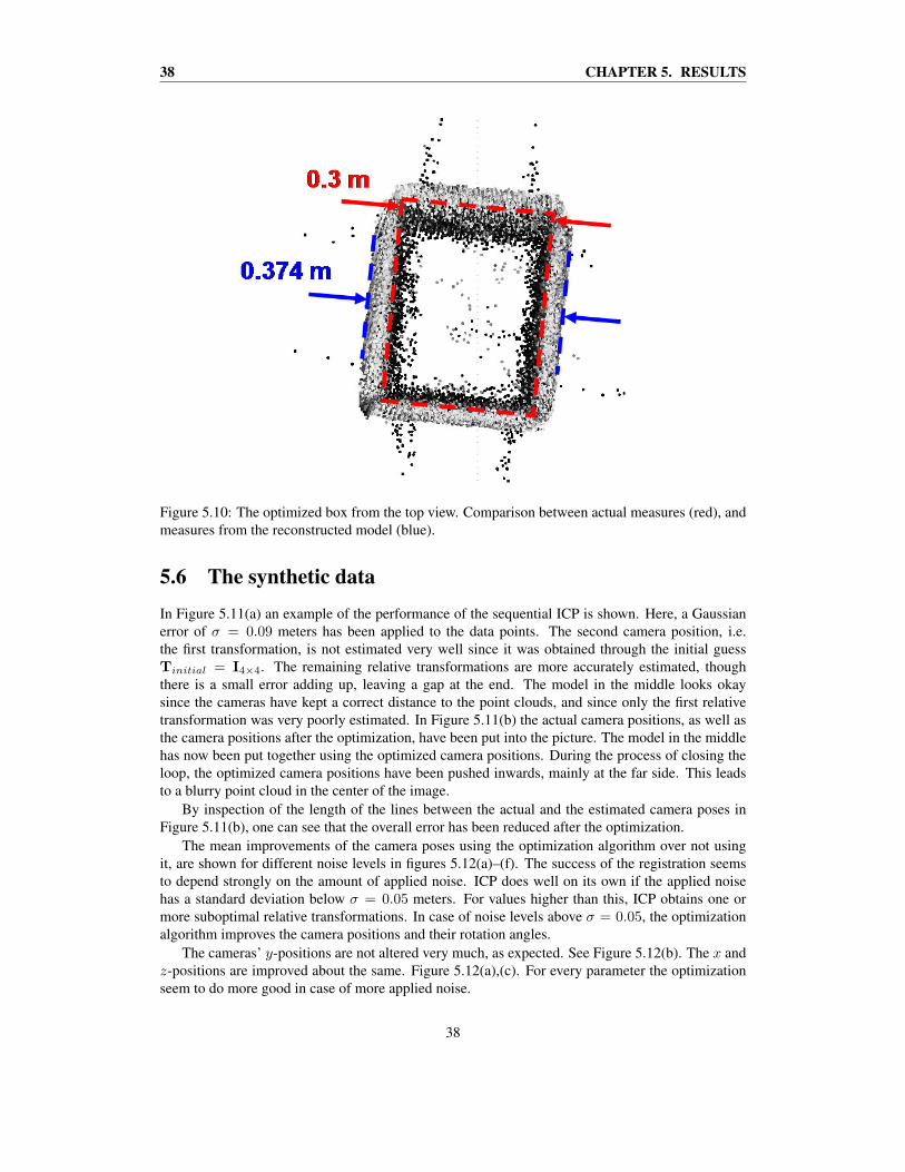
5.1 Translation of the camera aiming at an office desk. . . . . . . . . . . . . . . . . . 325.2 Approximative cumulative error in y and z-position of the camera. . . . . . . . . . 335.3 Values of the function being minimized, equation 2.10, during the optimization. . . 335.4 The reconstructed room with chairs . . . . . . . . . . . . . . . . . . . . . . . . . 345.5 A close-up on the camera positions from the reconstructed room with chairs . . . . 355.6 Approximative cumulative error in x, y and z-position of the camera. . . . . . . . . 355.7 The reconstructed empty room . . . . . . . . . . . . . . . . . . . . . . . . . . . . 365.8 Reconstruction of a human torso. . . . . . . . . . . . . . . . . . . . . . . . . . . . 375.9 Reconstruction of a non-cubic box. . . . . . . . . . . . . . . . . . . . . . . . . . . 375.10 The optimized box from the top view. Comparison between actual measures (red),

and measures from the reconstructed model (blue). . . . . . . . . . . . . . . . . . 385.11 Registration of the synthetic data for σ = 0.09 meters. . . . . . . . . . . . . . . . 395.12 The mean camera pose improvement after the optimization for different noise levels. 41

viii

Chapter 1

Introduction

1.1 Background

Laser scanners and Time of Flight (ToF) cameras can be used to measure huge amounts of 3Dcoordinates in a short period of time. This data can be used to reconstruct objects or areas if scansare taken from multiple angles. Since the 3D coordinates are relative to the scanning device, onehas to eventually move all points into the same coordinate system to make the model complete. Thisfusing of point clouds are often referred to as registration.

Registration can be made from aerial laser scans or aerial photography (Ronnholm et al., 2008).Reconstruction of buildings can be made to create digital maps in for instance Google Earth1, BingMaps2 or for machine simulators and realistic computer games (Bostrom et al., 2008; Gruen andAkca, 2005; Akca, 2007). Maps can be made using mobile robots in unknown and possibly haz-ardous environments for example in underground mining (Magnusson, 2006). A technique calledSimultaneous Localization And Mapping (SLAM), is often used by robots and autonomous vehiclesto build up such a map (Prusak et al., 2008; Nuchter et al., 2007; Borrmann et al., 2008).

Reconstruction of organs within the medical field can be made using data from computed tomog-raphy (CT) (Almhdie et al., 2007). Scans are used to digitize famous sculptures and monuments (Baeand Lichti, 2008). In addition to the above mentioned, there are also a variety of other applicationslinked to registration through the field of object recognition in 3D (Mian et al., 2006).

The usual source of data for reconstruction has in the past come from laser scanners becausethey give accurate measurements and provide a very dense set of points in each scan. Measurementaccuracies can be as good as <5 mm at a few hundred meters distance (Laser Scanner Survey 2005).

Stereo camera systems have also been used previously (Fors Nilsson and Grundberg, 2009).Recently it has been shown that ToF cameras can be accurate enough for registration. Artner (2009)showed that accuracies of a few centimeters can be obtained within a few meters if the camera is notmoving so fast.

Optronic3 is a service company within the field of optronics located in Skelleftea, Sweden. Theyfocus on integrated development and manufacturing of products for the industry. Optronic developsToF cameras based on Canesta’s4 3D-sensors in conjunction with the newly launched company,Fotonic5. Both companies see 3D-reconstruction as one possible application of their cameras in the

1http://earth.google.com/2http://www.microsoft.com/maps/3http://www.optronic.se/4http://canesta.com/5http://www.fotonic.com/

1

2 CHAPTER 1. INTRODUCTION

future.

1.2 Aims

The aim of this master’s thesis is to survey the literature and study at least two registration methodsbased on data from at least one ToF camera. The idea is to show how ToF cameras can be used forthe registration of point clouds to create 3D reconstructed environments and objects.

1.3 Related Work

There are quite a few algorithms used for registration of 3D-point clouds. The most famous isundoubtedly the Iterative Closest Point (ICP), which has been thoroughly investigated since it wasintroduced by Besl and McKay (1992) and Chen and Medioni (1992). The original version of ICPcalculates point correspondences and tries to minimize the total Euclidean distance between all thosepoints. This is done by iteratively applying different rotations and translations between point cloudsto find the best fit. The original algorithm assumes that there are no outliers and that every point inthe new dataset has a valid correspondence in the model.

ICP has a myriad of variants which have been developed over the years to suite different typesof inputs, e.g. intensity images are provided by many laser scanners and ToF cameras. Smith et al.(2008) and Barnea and Filin (2008) used ICP together with the Scale-Invariant Feature Transform(SIFT, Lowe (1999, 2004)). SIFT is used to find matching keypoints in images from different angles.These points can be used to estimate the transformation between two camera positions.

Another method that can be used to compute starting guesses for the camera movement betweentwo viewpoints, is RANdom SAmple Consensus (RANSAC, Fischler and Bolles (1981)). RANSAChas been used by several researchers in the past (Mure Dubois and Hugli, 2008; Smith et al., 2008;Barnea and Filin, 2008; Bae and Lichti, 2008).

The Iterative Closest Compatible Point (ICCP) introduced by Godin et al. (1994), reduces thesearch space compared to the original ICP. Only the distance between “compatible” points, thosewith similar attributes, e.g. color, are minimized. Iterative Closest Points using Invariant Features(ICPIF) was introduced by Sharp et al. (2000). It chooses point correspondences as the closest oneswith respect to a weighted linear combination of positional and feature distances. One invariantfeature is for example curvature.

The regular approach to registering multiple views is to first register views pairwise. This isusually followed by some kind of refinement. Bergevin et al. (1996) proposed a method whichminimizes the registration errors of all views simultaneously. This distributes the error between theframes. Williams and Bennamoun (2001) and Castellani et al. (2002) built their own registrationmethods based on the same principles.

Borrmann et al. (2008) presented a technique to match laser scans globally by minimizing aglobal error function. The closely related method aprxICP was explained and experimentally testedon ToF camera range images in the master’s thesis of Artner (2009).

Chetverikov et al. (2005) proposed a version called the Trimmed ICP (TrICP). This method wasbetter at coping with erroneous data than its predecessors, according to the author. The TrICP usesLeast Trimmed Squares (LTS) and also estimates a degree of overlap between frames to make theregistration more robust with respect to outliers.

Almhdie et al. (2007) used a comprehensive lookup matrix in the point matching step to en-hance the overall ICP performance. A method called Comprehensive ICP (CICP) was proposed andevaluated on medical images from tomography.

2

1.3. RELATED WORK 3

A thorough review of different approaches for speeding up the convergence of the ICP can befound in Rusinkiewicz and Levoy (2001).

Other, non-ICP registration algorithms include the methods proposed by Pottmann et al. (2004);Gruen and Akca (2005); Akca (2007); Akca and Gruen (2007).

A more extensive review on different registration methods within different fields can be foundin Gruen and Akca (2005). A few additional registration methods are also presented in Magnusson(2006).

The above mentioned articles are a summarization of the most influential research made up tilltoday. The literature study has given me a shallow overview of the methods used in different areasof applications.

3

4 CHAPTER 1. INTRODUCTION

4

Chapter 2

Theory

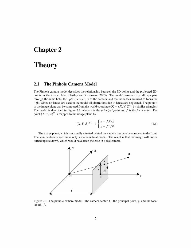
2.1 The Pinhole Camera ModelThe Pinhole camera model describes the relationship between the 3D-points and the projected 2D-points in the image plane (Hartley and Zisserman, 2003). The model assumes that all rays passthrough the same hole, the optical center, C of the camera, and that no lenses are used to focus thelight. Since no lenses are used in the model all aberrations due to lenses are neglected. The point xin the image plane can be computed from the world coordinate X = (X,Y, Z)T by similar triangles.The model is described in Figure 2.1, where p is the principal point and f is the focal point. Thepoint (X,Y, Z)T is mapped to the image plane by

(X,Y, Z)T −→

{x = fX/Z

y = fY/Z.(2.1)

The image plane, which is normally situated behind the camera has here been moved to the front.That can be done since this is only a mathematical model. The result is that the image will not beturned upside down, which would have been the case in a real camera.

Z

X

x

XY

C p

xy

f

Figure 2.1: The pinhole camera model. The camera center, C, the principal point, p, and the focallength, f .

5

6 CHAPTER 2. THEORY

roll pitch

ZX

Y

yaw

Figure 2.2: The SR4000 ToF camera. Arrows are showing the right-handed coordinate system andthe direction of the X,Y and Z-axis, as well as the angles of rotation; roll, pitch and yaw.

2.2 ToF camerasTime of Flight cameras can be used to measure distance to a vast number of points at the same time(SR4000 Manual, 2009). The frame rate of ToF cameras are typically around 30 fps which allowsfor range image acquisition during movement. Though, the exposure time, and thus the frame rate,need often be changed to suit the particular scene. The ToF camera that came to be used for dataacquisition was the Mesa SwissRanger 4000. This camera, together with its coordinate axes can beseen in Figure 2.2.

Next to the camera lens there are usually some Light Emitting Diodes, (LEDs) or Laser diodes,which are emitting a modulated light signal. The light is reflected back from the objects in thescene and is detected by the sensor in camera. By knowing the speed of light c, the distances can becalculated. The signal Sij , received at the pixel (i, j) of the CCD/CMOS sensor, can be described byits amplitude Aij and its phase φij (Mure Dubois and Hugli, 2008). The range rij , i.e. the distanceto a point in space, is directly proportional to the phase and can be calculated by

rij =c

4πf· φij , Sij = Aij · eiφij , (2.2)

where the i in front of φ, is the imaginary number√−1.

The conversion from range to x, y and z-values can be done by adapting the pinhole cameramodel. If we call the focal length f , the pixel shift (dx, dy) and define the normalized pixel coordi-nates (Xc, Yc), which are pixel coordinates relative to the camera center. Neglecting lens distortion,the Cartesian coordinates can according to Mure Dubois and Hugli (2008) be computed as

z = r · f√f2 + (Xcdx)2 + (Ycdy)2

(2.3)

x = z · Xcdxf

(2.4)

y = z · Ycdyf

. (2.5)

6

2.3. RIGID BODY TRANSFORMATIONS 7

2.3 Rigid body transformationsA rigid body transformation in 3D has six degrees of freedom, three rotation- and three translationparameters. Rigid body means that the proportions of the “body”, e.g. point cloud, lines et cetera,are preserved. A 4 × 4 transformation matrix can be constructed which moves the 3D data in onestep. If a 3D point is represented by a homogeneous 4-vector, x = [x, y, z, 1]T , the transformationmatrix is on the form

T =

[R t0T 1

],

where R is a 3× 3 orthogonal rotation matrix and t is a 3× 1 translation vector.The rotations around the different axes are defined as

Rx =

1 0 00 cos θ − sin θ0 sin θ cos θ

,Ry =

cos θ 0 sin θ0 1 0

− sin θ 0 cos θ

,Rz =

cos θ − sin θ 0sin θ cos θ 00 0 1

.

The inverse of a rotation, R−1 = RT . This is a property of othogonal matrices such as forexample the rotation matrix. The inverse of a transformation with both rotation and translation is

T−1 =

[RT −RT t0T 1

].

To move the points in Xworld into the coordinate system of the camera, Xcam, the transforma-tion Tcam can be applied

Xcam = TcamXworld =

[Rcam −RcamC0T 1

]︸︷︷︸

Tcam

Xworld,

where C = [x, y, z]T is the position of the camera center and Rcam describes the orientation of theworld with respect to the camera.

2.4 QuaternionsThere are a number of ways to represent rotations. Quaternions are often used as a representationof rotation angles within the area of multi-image registration instead of the otherwise commonlyused Euler representation. Euler rotations are made by consecutively rotating around the x, y andz-axis. The rotations about these axes are often referred to by the aerospace terms pitch, yaw androll. Quaternions are as opposed to Euler angles represented using four dimensions (The Matrix andQuaternions FAQ, 2003). This avoids the problem known as ”gimbal-lock”, and performs rotationsin a smooth and continuous way.

Quaternions possess a number of other nice qualities. Wheeler and Ikeuchi (1995) states a largenumber of these qualities, and a few of them are

– Quaternions need only be multiplied to accumulate the effects of composed rotations.

– An inverse rotation with quaternions is done simply by negating three components of thequaternion.

– The rotation between two rotations can be computed by multiplying one quaternion with theinverse of the other.

7

8 CHAPTER 2. THEORY

(u,v,w)

s

i

j

k

Figure 2.3: Schematic illustration of the quaternion angle representation.

– Quaternions are particularly suitable for iterative gradient- or Jacobian-based search for rota-tion and translation.

It is difficult to visually describe the quaternions, since they consist of three imaginary numbersand one rotation. However, one way is shown in Figure 2.3, where the quaternion q = [u, v, w, s] iscomputed as

s = cos(ϕ/2)

u = i(x sin(ϕ/2))

v = j(y sin(ϕ/2))

w = k(z sin(ϕ/2)),

and ϕ is the angle in the axis angle representation. Thus, s is the angle of rotation about the axiswith direction (u, v, w).

2.5 Methods for estimating transformations

ICP and several other registration methods need an approximate initial guess on the transformationsin order not to converge to the wrong local minima. Within SLAM there are usually some odometryattached to the robot/camera, to provide the registration method with initial pose estimates. Though,there are a few alternatives. If 2D-images are available, e.g. from a digital camera attached to therobot, or from an amplitude image of a range camera. Then the strategy of obtaining a transformationconsists of a few steps.

1. Finding keypoints in two images.

2. Matching corresponding keypoints in the images.

3. Performing a triangulation to obtain the 3D coordinates of these points.

With enough matched 3D points, a rigid body transformation can be computed (Hartley and Zisser-man, 2003).

8

2.6. CALIBRATION 9

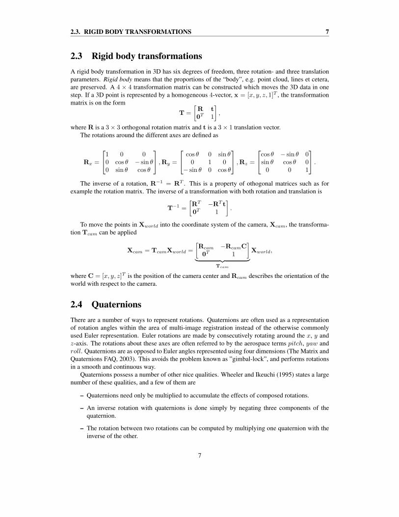
Figure 2.4: Matched SIFT keypoints between two amplitude images of a ToF camera.

2.5.1 SIFTScale-Invariant Feature Transform (SIFT) is a method used for finding certain feature points in2D-images. At these points, feature vectors are computed, each of which is invariant to imagetranslation, scaling, and rotation. The feature vectors are also partially invariant to illuminationchanges and robust to local geometric distortion. An example where SIFT matches have been foundbetween two amplitude images of a ToF camera can be seen in Figure 2.4.

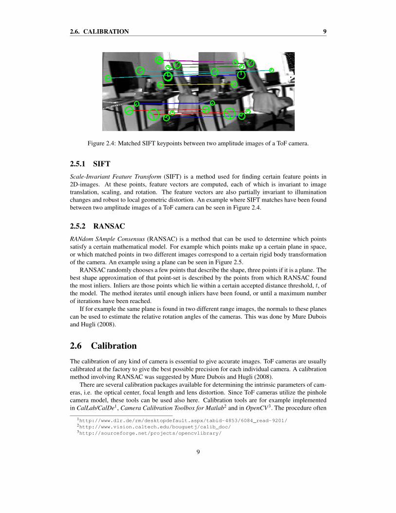
2.5.2 RANSACRANdom SAmple Consensus (RANSAC) is a method that can be used to determine which pointssatisfy a certain mathematical model. For example which points make up a certain plane in space,or which matched points in two different images correspond to a certain rigid body transformationof the camera. An example using a plane can be seen in Figure 2.5.

RANSAC randomly chooses a few points that describe the shape, three points if it is a plane. Thebest shape approximation of that point-set is described by the points from which RANSAC foundthe most inliers. Inliers are those points which lie within a certain accepted distance threshold, t, ofthe model. The method iterates until enough inliers have been found, or until a maximum numberof iterations have been reached.

If for example the same plane is found in two different range images, the normals to these planescan be used to estimate the relative rotation angles of the cameras. This was done by Mure Duboisand Hugli (2008).

2.6 CalibrationThe calibration of any kind of camera is essential to give accurate images. ToF cameras are usuallycalibrated at the factory to give the best possible precision for each individual camera. A calibrationmethod involving RANSAC was suggested by Mure Dubois and Hugli (2008).

There are several calibration packages available for determining the intrinsic parameters of cam-eras, i.e. the optical center, focal length and lens distortion. Since ToF cameras utilize the pinholecamera model, these tools can be used also here. Calibration tools are for example implementedin CalLab/CalDe1, Camera Calibration Toolbox for Matlab2 and in OpenCV3. The procedure often

1http://www.dlr.de/rm/desktopdefault.aspx/tabid-4853/6084_read-9201/2http://www.vision.caltech.edu/bouguetj/calib_doc/3http://sourceforge.net/projects/opencvlibrary/

9

10 CHAPTER 2. THEORY

t

Figure 2.5: Point fitting to a plane with RANSAC. Inliers, i.e. accepted points, marked by greendots. Points further away than the distance treshold, t, marked by red dots.

involves taking images at a calibration grid, e.g. a checker-board pattern, at different distances andangles. Fuchs and Hirzinger (2008) used the CalLab/CalDe toolbox and obtained a mean precisionof 1 mm and 2◦ with an IFM O3D100 ToF camera.

2.7 ToF camera errorsToF cameras that are in movement produce a lot of erroneous coordinate points. Also, since thepoint clouds are so dense, some kind of filtering is recommended to be applied before registration.

According to May et al. (2009) and Nordqvist (2010) there are a few systematic and non-systematic errors which the ToF cameras are suffering from. These can be countered by differentkinds of filters and calibration.

Non-systematic errors

– Low signal-to-noise ratio. This error varies between cameras and scenes, e.g. some camerashave a stronger emitted signal than others. Furthermore the strength of the returning signaldepends on the distance to the objects in the scene and the reflectance of their surfaces.

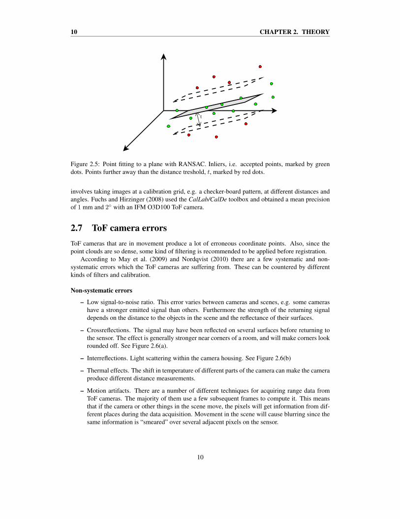
– Crossreflections. The signal may have been reflected on several surfaces before returning tothe sensor. The effect is generally stronger near corners of a room, and will make corners lookrounded off. See Figure 2.6(a).

– Interreflections. Light scattering within the camera housing. See Figure 2.6(b)

– Thermal effects. The shift in temperature of different parts of the camera can make the cameraproduce different distance measurements.

– Motion artifacts. There are a number of different techniques for acquiring range data fromToF cameras. The majority of them use a few subsequent frames to compute it. This meansthat if the camera or other things in the scene move, the pixels will get information from dif-ferent places during the data acquisition. Movement in the scene will cause blurring since thesame information is “smeared” over several adjacent pixels on the sensor.

10

2.8. FILTERING 11

(a)

Lens

Sensor

(b)

Figure 2.6: Two common artifacts of ToF cameras. (a) Crossreflections, i.e. multiple reflections.Light may have been reflected against more than one surface, creating a faulty distance measure.(b) Interreflections, i.e. internal light scattering. Light can have been reflected against the camerahousing or against the lens.

Systematic errors

– The assumption that the signal is sinusoidal is only approximately true. This leads to adistance-related error.

– The non-linearity of the electronic components of the pixels lead to an error in determiningthe amplitude.

– Since the pixels on the sensor are connected in series, the pixels with a longer distance to asignal generator will have a larger measurement offset.

The systematic errors can be tackled by a depth calibration to fit the pinhole camera model.A more in-depth explanation of some of these shortcomings can be found in Fuchs and Hirzinger(2008).

2.8 FilteringFiltering is often used to improve the data returned by ToF cameras. Filters can both be in the formof passive components within the camera, or as software implemented for post-processing. Thesoftware filters can be implemented within the camera itself or in a host computer.

ToF cameras usually have an optical filter which removes light with other wavelengths than itsoperating near-infrared (NIR) wavelength. Without this particular filter, ToF cameras could not beused in direct sunlight.

Among software filtering techniques, the signal amplitude threshold is one of the most common.A pixel receiving a strong signal without being saturated is likely to have received a good distancemeasurement. Measurements from pixels on the sensor which have been under- or oversaturated arelikely to be erroneous. Surfaces which have a high NIR-reflectance often return a strong signal andthus probably a good measurement. The illumination from the camera decreases with the square of

11


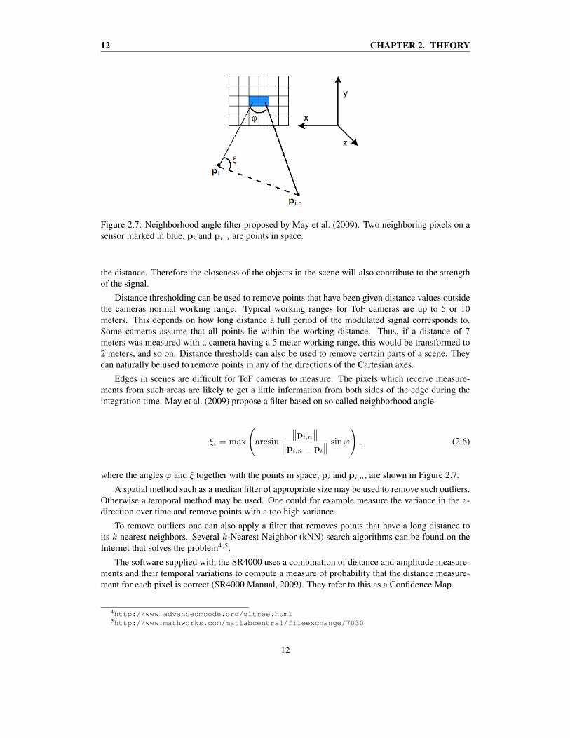
Figure 2.7: Neighborhood angle filter proposed by May et al. (2009). Two neighboring pixels on asensor marked in blue, pi and pi,n are points in space.

the distance. Therefore the closeness of the objects in the scene will also contribute to the strengthof the signal.

Distance thresholding can be used to remove points that have been given distance values outsidethe cameras normal working range. Typical working ranges for ToF cameras are up to 5 or 10meters. This depends on how long distance a full period of the modulated signal corresponds to.Some cameras assume that all points lie within the working distance. Thus, if a distance of 7meters was measured with a camera having a 5 meter working range, this would be transformed to2 meters, and so on. Distance thresholds can also be used to remove certain parts of a scene. Theycan naturally be used to remove points in any of the directions of the Cartesian axes.

Edges in scenes are difficult for ToF cameras to measure. The pixels which receive measure-ments from such areas are likely to get a little information from both sides of the edge during theintegration time. May et al. (2009) propose a filter based on so called neighborhood angle

ξi = max

(arcsin

∥∥pi,n

∥∥∥∥pi,n − pi

∥∥ sinφ

), (2.6)

where the angles φ and ξ together with the points in space, pi and pi,n, are shown in Figure 2.7.

A spatial method such as a median filter of appropriate size may be used to remove such outliers.Otherwise a temporal method may be used. One could for example measure the variance in the z-direction over time and remove points with a too high variance.

To remove outliers one can also apply a filter that removes points that have a long distance toits k nearest neighbors. Several k-Nearest Neighbor (kNN) search algorithms can be found on theInternet that solves the problem4,5.

The software supplied with the SR4000 uses a combination of distance and amplitude measure-ments and their temporal variations to compute a measure of probability that the distance measure-ment for each pixel is correct (SR4000 Manual, 2009). They refer to this as a Confidence Map.

4http://www.advancedmcode.org/gltree.html5http://www.mathworks.com/matlabcentral/fileexchange/7030

12

2.9. ICP 13

2.9 ICPICP is an algorithm employed to minimize the difference between two point sets. The purpose forusing ICP is often to build up 3D models which later can be used for different purposes. If thealgorithm is implemented in an efficient way on a powerful enough computer, the algorithm couldbe used in real time.

The first dataset is usually called M = {m1 . . .mNM}, for model, and the second D =

{d1 . . . dND}, for dataset. ICP normally consists of a few basic steps.

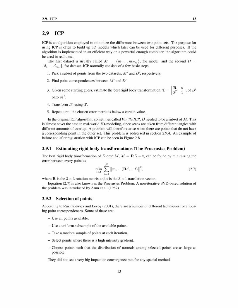
1. Pick a subset of points from the two datasets, M ′ and D′, respectively.

2. Find point correspondences between M ′ and D′.

3. Given some starting guess, estimate the best rigid body transformation, T =

[R t0T 1

], of D′

onto M ′.

4. Transform D′ using T.

5. Repeat until the chosen error metric is below a certain value.

In the original ICP algorithm, sometimes called Vanilla ICP, D needed to be a subset of M . Thisis almost never the case in real-world 3D-modeling, since scans are taken from different angles withdifferent amounts of overlap. A problem will therefore arise when there are points that do not havea corresponding point in the other set. This problem is addressed in section 2.9.4. An example ofbefore and after registration with ICP can be seen in Figure 2.8.

2.9.1 Estimating rigid body transformations (The Procrustes Problem)The best rigid body transformation of D onto M , M = RD + t, can be found by minimizing theerror between every point as

minR,t

N∑i=1

∥∥mi − (Rdi + t)∥∥2, (2.7)

where R is the 3× 3 rotation matrix and t is the 3× 1 translation vector.Equation (2.7) is also known as the Procrustes Problem. A non-iterative SVD-based solution of

the problem was introduced by Arun et al. (1987).

2.9.2 Selection of pointsAccording to Rusinkiewicz and Levoy (2001), there are a number of different techniques for choos-ing point correspondences. Some of these are:

– Use all points available.

– Use a uniform subsample of the available points.

– Take a random sample of points at each iteration.

– Select points where there is a high intensity gradient.

– Choose points such that the distribution of normals among selected points are as large aspossible.

They did not see a very big impact on convergence rate for any special method.

13


Figure 2.8: ICP alignment of a dataset onto a model. Dataset position before registration, blue dots.Dataset position after registration, red dots.

2.9.3 How to match points

– Find the closest point in the other mesh for example using a search tree.

– Find the intersection between the source point and the destination surface with the directionnormal to the source surface. This is called “Normal shooting”.

– Project the source point onto the destination mesh from the point of view of the destinationmesh’s range camera. This is also called “Reverse calibration”.

– Project the source point onto the destination mesh, then perform a search in the destinationrange image.

Rusinkiewicz and Levoy (2001) propose a projection-based algorithm to produce point corre-spondences together with a point-to-plane error metric.

2.9.4 Rejection of point pairs

Since usually only a part of the datasets overlap, one needs some rule to reject points which doesnot have a corresponding point in the other set. A number of heuristics can be deployed to solve theproblem, as stated in Williams and Bennamoun (2001).

– Maximum match distance. Reject any matches between points separated by a distance greaterthan a threshold value.

14

2.10. LOOP CLOSING AND ERROR RELAXATION 15

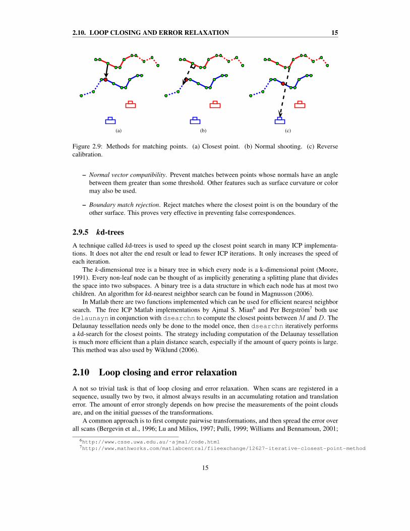
(a) (b) (c)

Figure 2.9: Methods for matching points. (a) Closest point. (b) Normal shooting. (c) Reversecalibration.

– Normal vector compatibility. Prevent matches between points whose normals have an anglebetween them greater than some threshold. Other features such as surface curvature or colormay also be used.

– Boundary match rejection. Reject matches where the closest point is on the boundary of theother surface. This proves very effective in preventing false correspondences.

2.9.5 kd-treesA technique called kd-trees is used to speed up the closest point search in many ICP implementa-tions. It does not alter the end result or lead to fewer ICP iterations. It only increases the speed ofeach iteration.

The k-dimensional tree is a binary tree in which every node is a k-dimensional point (Moore,1991). Every non-leaf node can be thought of as implicitly generating a splitting plane that dividesthe space into two subspaces. A binary tree is a data structure in which each node has at most twochildren. An algorithm for kd-nearest neighbor search can be found in Magnusson (2006).

In Matlab there are two functions implemented which can be used for efficient nearest neighborsearch. The free ICP Matlab implementations by Ajmal S. Mian6 and Per Bergstrom7 both usedelaunayn in conjunction with dsearchn to compute the closest points between M and D. TheDelaunay tessellation needs only be done to the model once, then dsearchn iteratively performsa kd-search for the closest points. The strategy including computation of the Delaunay tessellationis much more efficient than a plain distance search, especially if the amount of query points is large.This method was also used by Wiklund (2006).

2.10 Loop closing and error relaxationA not so trivial task is that of loop closing and error relaxation. When scans are registered in asequence, usually two by two, it almost always results in an accumulating rotation and translationerror. The amount of error strongly depends on how precise the measurements of the point cloudsare, and on the initial guesses of the transformations.

A common approach is to first compute pairwise transformations, and then spread the error overall scans (Bergevin et al., 1996; Lu and Milios, 1997; Pulli, 1999; Williams and Bennamoun, 2001;

6http://www.csse.uwa.edu.au/˜ajmal/code.html7http://www.mathworks.com/matlabcentral/fileexchange/12627-iterative-closest-point-method

15


V a

V b

V c

V d

Figure 2.10: Graph edges between views, i.e. cameras, which are close enough.

Castellani et al., 2002; Fusiello et al., 2002; Thrun and Montemerlo, 2005; Borrmann et al., 2008;Olson, 2008; May et al., 2009; Artner, 2009).

A graph is usually built to keep track of all views, i.e. camera poses, see Figure 2.10. InBorrmann et al. (2008) views were connected by an edge if they were close enough to each otherspatially. Views that are close together can be assumed to have some overlap. The detection of thesekinds of loops can of course be done manually, but this can be a tedious job if there are a lot of scansand loops.

A rough pose estimate can be obtained through e.g. the pairwise ICP, odometry equipmentattached to the camera, or by computing the rigid body transformations from features in the intensityimages.

In the GraphSLAM approach of Thrun and Montemerlo (2005), an extended version of equation2.7 is used. The graph of the overlapping views,

GV = ({Va → Vb}, {Va → Vc}, {Vb → Vc}, . . . ),

is now used to minimize the error between corresponding points in all overlapping views. The errorto be minimized becomes

E(R, t) =∑j→k

∑i

∥∥ (Rjmi + tj)︸︷︷︸Vj

− (Rkdi + tk)︸︷︷︸Vk

∥∥2 . (2.8)

A relatively concise explanation of a 6D SLAM, globally consistent scan matching strategy, canbe found in Borrmann et al. (2008). They extended Lu and Milios (1997) method to 6 degrees offreedom. It iteratively minimizes the point-to-point error in overlapping views and spreads the errorobtained from the detected loops over the estimated poses. This method involves computing thecovariance matrices between these views. An enhancement which speeded up the loop closing stepwas later added by Sprickerhof et al. (2009)8.

Another, less complex, approach which does not involve the computation of covariance matriceswas proposed by Castellani et al. (2002). Following the notation used in the article, the completealgorithm for registering multiple views can be summarized as:

1. Compute the transformations, Gi,j , between all overlapping views with pairwise ICP, where

G =

[R t0T 1

],

and Gi,j registers view j onto view i.

8The 6D-SLAM software is open source and can be found at http://slam6d.sourceforge.net/.

16

2.10. LOOP CLOSING AND ERROR RELAXATION 17

2. If the registration was good, store the transformation matrix Gi,j , otherwise reject it.

3. Compute the starting guesses, Gi, for transforming the views, Vi, to the coordinate systemof V1 according to

Gi =i∏

j=2

Gj−1,j (2.9)

4. Minimize the objective function9

min∑i,j

((angle(RiRi,j(Rj)T )

σα

)2

+

(∥∥Riti,j + ti − tj∥∥

σt

)2), (2.10)

where angle(. . . ) returns the screw axis angle for a given rotation matrix, and σα and σt arenormalization factors (Soderkvist and Wedin, 1994). In Fusiello et al. (2002) the normaliza-tion factors were set to σα = π, and σt =

∥∥ti∥∥.

At each step enforce orthogonality of the rotation matrix according to

R(q) =1

q · qRu(q), (2.11)

where q = [u, v, w, s] is a quaternion and the conversion to an Euclidean rotation matrix isdone by

Ru(q) =

s2 + u2 − v2 − w2 2(uv − sw) 2(uw + sv)2(uv + sw) s2 − u2 + v2 − w2 2(vw − su)2(uw − sv) 2(vw + su) s2 − u2 − v2 + w2

(2.12)

5. Apply all transformations, Gi, to the views, Vi.

9The minimization can be done with Matlab’s lsqnonlin or fmincon.

17


18

Chapter 3

Implementation

3.1 Preprocessing

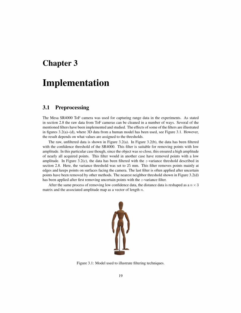
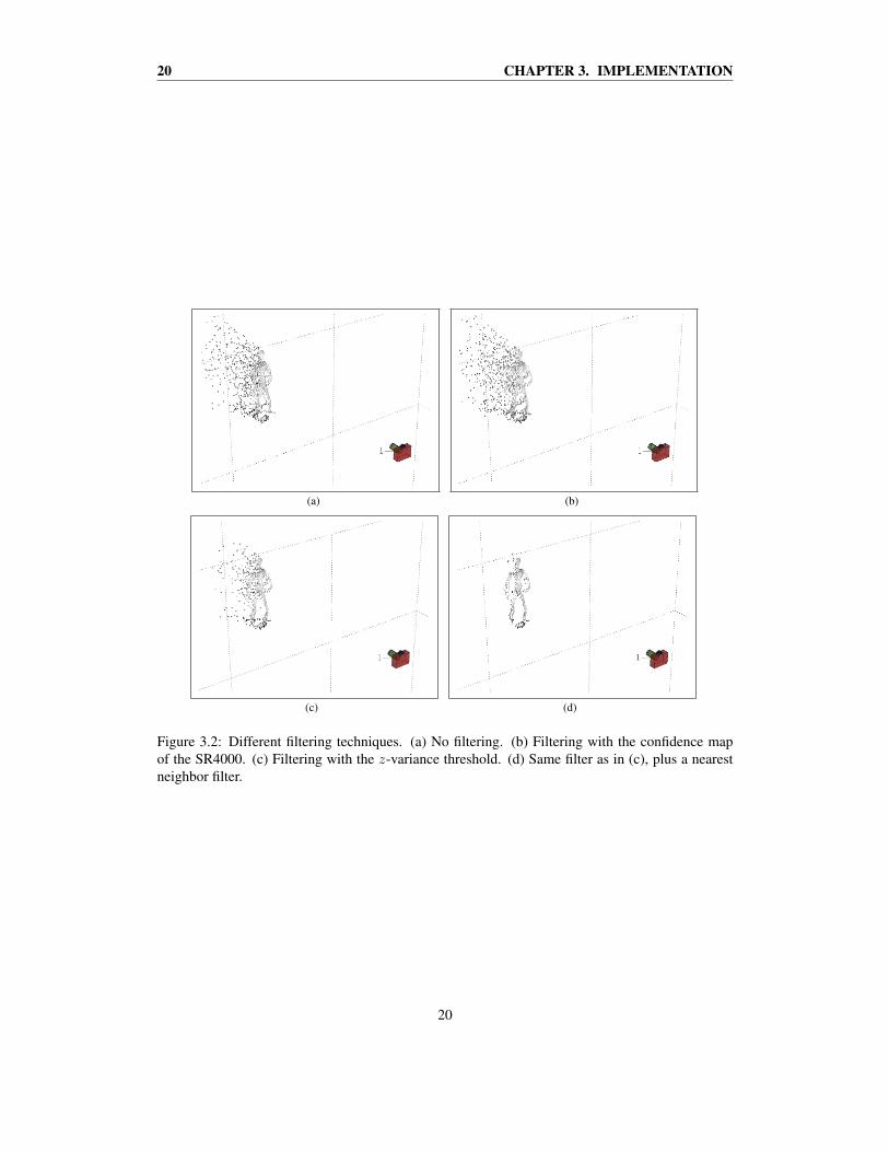
The Mesa SR4000 ToF camera was used for capturing range data in the experiments. As statedin section 2.8 the raw data from ToF cameras can be cleaned in a number of ways. Several of thementioned filters have been implemented and studied. The effects of some of the filters are illustratedin figures 3.2(a)–(d), where 3D data from a human model has been used, see Figure 3.1. However,the result depends on what values are assigned to the thresholds.

The raw, unfiltered data is shown in Figure 3.2(a). In Figure 3.2(b), the data has been filteredwith the confidence threshold of the SR4000. This filter is suitable for removing points with lowamplitude. In this particular case though, since the object was so close, this ensured a high amplitudeof nearly all acquired points. This filter would in another case have removed points with a lowamplitude. In Figure 3.2(c), the data has been filtered with the z-variance threshold described insection 2.8. Here, the variance threshold was set to 25 mm. This filter removes points mainly atedges and keeps points on surfaces facing the camera. The last filter is often applied after uncertainpoints have been removed by other methods. The nearest neighbor threshold shown in Figure 3.2(d)has been applied after first removing uncertain points with the z-variance filter.

After the same process of removing low confidence data, the distance data is reshaped as a n×3matrix and the associated amplitude map as a vector of length n.

Figure 3.1: Model used to illustrate filtering techniques.

19

20 CHAPTER 3. IMPLEMENTATION

(a) (b)

(c) (d)

Figure 3.2: Different filtering techniques. (a) No filtering. (b) Filtering with the confidence mapof the SR4000. (c) Filtering with the z-variance threshold. (d) Same filter as in (c), plus a nearestneighbor filter.

20

3.2. PAIRWISE ICP 21

3.2 Pairwise ICPAs a foundation for the pairwise ICP the implementation of Ajmal S. Mian1 has been used. Thecode solves the Procrustes problem and it is concise and understandable. As stated earlier, in section2.9, it takes in two datasets data1, data2, the resolution of the data, and registers the second intothe coordinate system of the first one. In addition to the registered data, the function also returns theapproximated rotation and translation together with the indices of the corresponding points, and anerror measure.

The function was modified to accept arbitrary starting guesses on the transformation T. Previ-ously, the function always assumed that Tinitial = I4×4. This meaning that the datasets needed tobe rather close initially, to be registered successfully. Moreover, the function was made to return thenumber of corresponding points, as that also is a good measure on how well the registration went.An algorithm of the basic pairwise ICP is shown below.

Algorithm 1: Pairwise ICP

1 while the number of corresponding points does not change do2 Compute the Delaunay tessellation of data1;3 for every point in data2 do4 Compute the closest point in data1;5 end6 Remove the points which have their corresponding point further away than 2 · res;7 if several points have the same corresponding point in data1 then8 Only keep the one with the shortest distance;9 end

10 Solve the Procrustes problem according to Arun et al. (1987);11 Apply the transformation to data2;12 if maximum number of iterations have been reached then13 Terminate;14 end15 end16 Re-run the above steps until the change in the error has been below a value ϵ, for k

iterations. The error is here computed as

E =∑ di

np · res,

where di is the distances between corresponding points and np is the total number ofpoints.

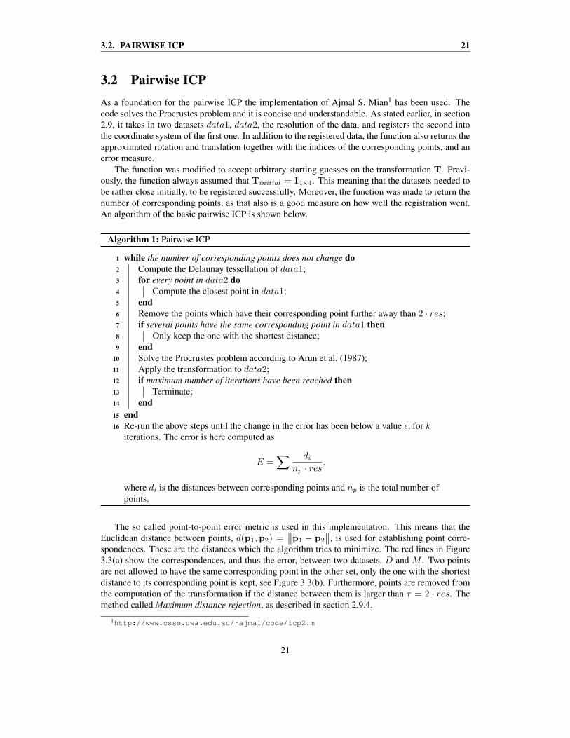
The so called point-to-point error metric is used in this implementation. This means that theEuclidean distance between points, d(p1,p2) =

∥∥p1 − p2

∥∥, is used for establishing point corre-spondences. These are the distances which the algorithm tries to minimize. The red lines in Figure3.3(a) show the correspondences, and thus the error, between two datasets, D and M . Two pointsare not allowed to have the same corresponding point in the other set, only the one with the shortestdistance to its corresponding point is kept, see Figure 3.3(b). Furthermore, points are removed fromthe computation of the transformation if the distance between them is larger than τ = 2 · res. Themethod called Maximum distance rejection, as described in section 2.9.4.

1http://www.csse.uwa.edu.au/˜ajmal/code/icp2.m

21


(a) (b)

Figure 3.3: The point-to-point method for determining corresponding points between datasets. (a)All point correspondences between D and M . (b) Point correspondences made unique throughshortest distance.

3.3 Multi-view registrationEvery frame taken by a regular ToF camera today consists of about 25 000 points. This means thatcomputing the transformation between point clouds using ICP would take a lot of time if the wholedatasets were used, especially when dealing with multi-view registration. A subset is thereforerecommended, and as in Rusinkiewicz and Levoy (2001), this was chosen to the simplest one, arandom subsample. Though the same subset was used through all ICP iterations. The number ofpoints used was taken to be 1000 for both M ′ and D′.

The pairwise rotations and translations of the point clouds are stored in a matrix for later use.The accumulated translations and rotations, that moves an arbitrary point cloud into the initial one’scoordinate system, are then calculated as

t = R · tnew + t; (3.1)R = R ·Rnew; (3.2)

The accumulated R:s are then converted to quaternions by Matlab’s function dcm2quat andstored together with t on the form

x0 = [q2T ; t2; q3T ; t3; . . . ; qnT ; tn].

The transformation {qi, ti} registers the i:th point cloud into the first one’s coordinate system.The vector x0 will be the starting guess for the upcoming global minimization, in which q1 and t1are not supplied since they are not supposed to change.

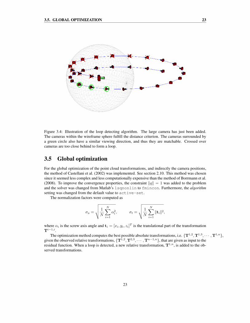
3.4 Loop closingA function was implemented that searches for cameras with possible overlap. The Euclidean dis-tances between the new camera position and all previous camera positions are calculated as well asthe differences in yaw angle (rotation around the cameras y-axis). If two cameras are close enoughand have approximately the same yaw angle, the cameras can be said to have possible overlap. Toconfirm that they have overlap, the pairwise ICP is used. If the error is low, and the amount ofcorresponding points is above a certain percentage of the total number of points, overlap is assumed.An example is shown in Figure 3.4.

22

3.5. GLOBAL OPTIMIZATION 23

Figure 3.4: Illustration of the loop detecting algorithm. The large camera has just been added.The cameras within the wireframe sphere fulfill the distance criterion. The cameras surrounded bya green circle also have a similar viewing direction, and thus they are matchable. Crossed overcameras are too close behind to form a loop.

3.5 Global optimizationFor the global optimization of the point cloud transformations, and indirectly the camera positions,the method of Castellani et al. (2002) was implemented. See section 2.10. This method was chosensince it seemed less complex and less computationally expensive than the method of Borrmann et al.(2008). To improve the convergence properties, the constraint ∥q∥ = 1 was added to the problemand the solver was changed from Matlab’s lsqnonlin to fmincon. Furthermore, the algorithmsetting was changed from the default value to active-set.

The normalization factors were computed as

σa =

√√√√ 1

N

N∑i=1

α2i , σt =

√√√√ 1

N

N∑i=1

∥ti∥2,

where αi is the screw axis angle and ti = [xi, yi, zi]T is the translational part of the transformation

Ti−1,i.The optimization method computes the best possible absolute transformations, i.e. {T1,2,T1,3, · · · ,T1,n},

given the observed relative transformations, {T1,2,T2,3, · · · ,Tn−1,n}, that are given as input to theresidual function. When a loop is detected, a new relative transformation, T1,n, is added to the ob-served transformations.

23


24

Chapter 4

Experiments

4.1 Test cases

A few test cases were constructed. These were:

1. Translation of the camera sideways 90 cm and back, along a rail.

2. Rotation of the camera 360◦ in a rectangular room with reference objects evenly spaced.

3. Rotation of the camera 360◦ in a room without reference objects.

4. Rotating a torso 360◦.

5. Rotating a non-cubic box 360◦.

6. Rotating synthetic data 360◦.

All data frames were filtered by the same method before the registration, except the syntheticdata, which was unfiltered. The confidence level 7/8 of the SR4000 was used together with theremoval of half of the points in each frame. The removed points had the largest mean distance totheir three nearest neighbors. In some of the cases, a distance threshold was used to remove pointswhich should not be part of the model.

Common to all test cases was also the integration time of the SR4000, which was set to 30milliseconds, yielding a frame rate of approximately 30 fps. Moreover, the resolution parameter ofthe ICP was set to 0.01 meters for all cases except for the case with the synthetic data, where it wasset to 1 meter.

Pairwise ICP was performed on sequential frames with two different types of initial guesses onthe relative transformations. The initial guess, Tinitial = I4×4. This approach assumes that M andD are close enough to be registered initially. The other type of initial guess, Tinitial = Tprevious,is where the guess on the upcoming transformation is obtained from the preceding pairwise ICP, andso on. Here, only the first initial guess of the sequence need to be Tinitial = I4×4.

After the transformation between the last and the first frame of the sequence, T1,n, had been ob-tained, the loop was closed using the method of Castellani et al. (2002). Sequences were constructedso that the camera would end up at approximately the same position as it started at. Detection ofthese loops was done manually by looking at amplitude images from the sequences.

25

26 CHAPTER 4. EXPERIMENTS

(a) (b)

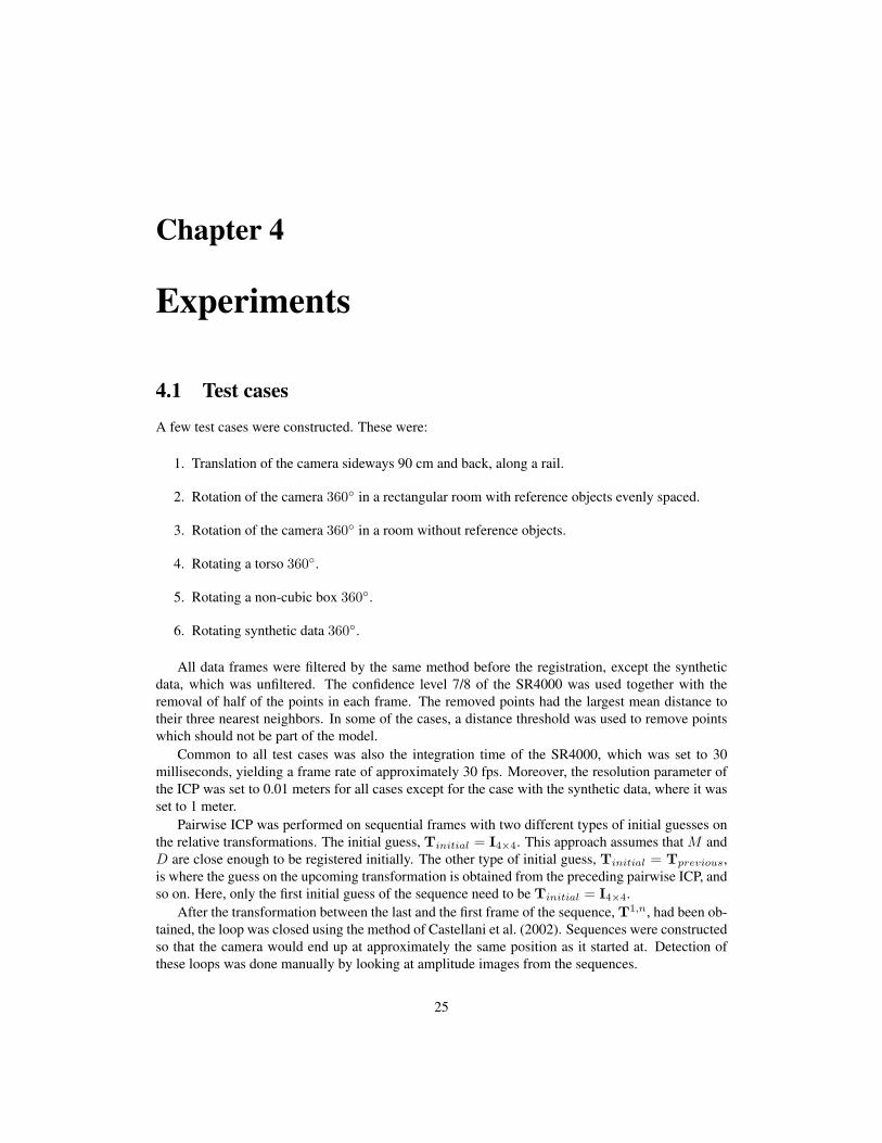
Figure 4.1: Translation of the camera. (a) The camera on a rail. (b) An arbitrarily chosen amplitudeimage from the data acquisition, aiming at an office desk, a chair and a plastic flower.

4.1.1 Translation of the camera

The camera was mounted on a rail, that made it possible to slide the camera back and forth by hand.It was aimed at an office desk, a chair and a plastic flower. Translation was made sideways 90 cm inthe camera’s positive x-direction and then back again. The camera mounted on the rail is shown inFigure 4.1(a). An arbitrarily chosen amplitude image is shown in Figure 4.1(b).

The sequence was captured in 315 frames, though, only every fifth frame was used in the regis-tration. Hence this sequence consists of 63 frames.

This was the only case where the initial guess on the transformation, Tinitial = I4×4, wastested. In the following experiments only the other type of initial guess is used.

No pose measurements were gathered during the data acquisition. To take manual measurementswould have been exhausting due to the vast number of frames. Though, the camera should not havemoved much in the y and z-direction. This is a consequence of the camera being mounted with thez-axis approximately perpendicular to the rail both horizontally and vertically. Thus, the cumulativeerror in the y and z-direction was calculated relative to the first camera pose.

4.1.2 Room with reference objects

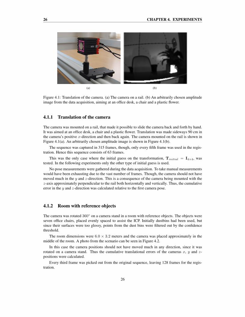
The camera was rotated 360◦ on a camera stand in a room with reference objects. The objects wereseven office chairs, placed evenly spaced to assist the ICP. Initially dustbins had been used, butsince their surfaces were too glossy, points from the dust bins were filtered out by the confidencethreshold.

The room dimensions were 6.0 × 3.2 meters and the camera was placed approximately in themiddle of the room. A photo from the scenario can be seen in Figure 4.2.

In this case the camera positions should not have moved much in any direction, since it wasrotated on a camera stand. Thus the cumulative translational errors of the cameras x, y and z-positions were calculated.

Every third frame was picked out from the original sequence, leaving 128 frames for the regis-tration.

26

4.1. TEST CASES 27

Figure 4.2: The room in which the rotation scenario was done. Chairs are placed evenly spaced asreference objects.

4.1.3 Empty room

To show the importance of proper reference objects when not using any odometry data, as in thiscase, the room was reconstructed without the chairs. The same room was used as in the previouscase. Here, every third frame was utilized, leaving 135 frames.

4.1.4 The torso

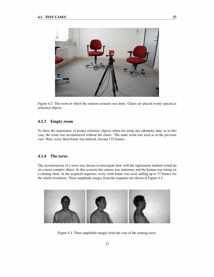
The reconstruction of a torso was chosen to investigate how well the registration method would doon a more complex object. In this scenario the camera was stationary and the human was sitting ona rotating chair. In the acquired sequence, every sixth frame was used, adding up to 37 frames forthe whole revolution. Three amplitude images from the sequence are shown in Figure 4.3.

Figure 4.3: Three amplitude images from the case of the rotating torso.

27


Figure 4.4: The box on a stand.

4.1.5 The boxThe scene with the rotating box was made to be able to get an actual measurement on how good theregistrations went. The box was chosen for its parallel and right angles as well as its other knowndimensions. The dimensions of the box were 300 × 300 × 400 mm. In this sequence, only everytenth frame was used. This, since the rotation speed of the box was slower than in the previousrotating cases. The number of frames were 57 for this revolution.

The surface of the box is matte white, which is essential to get high confidence points. The boxcan be seen in Figure 4.4.

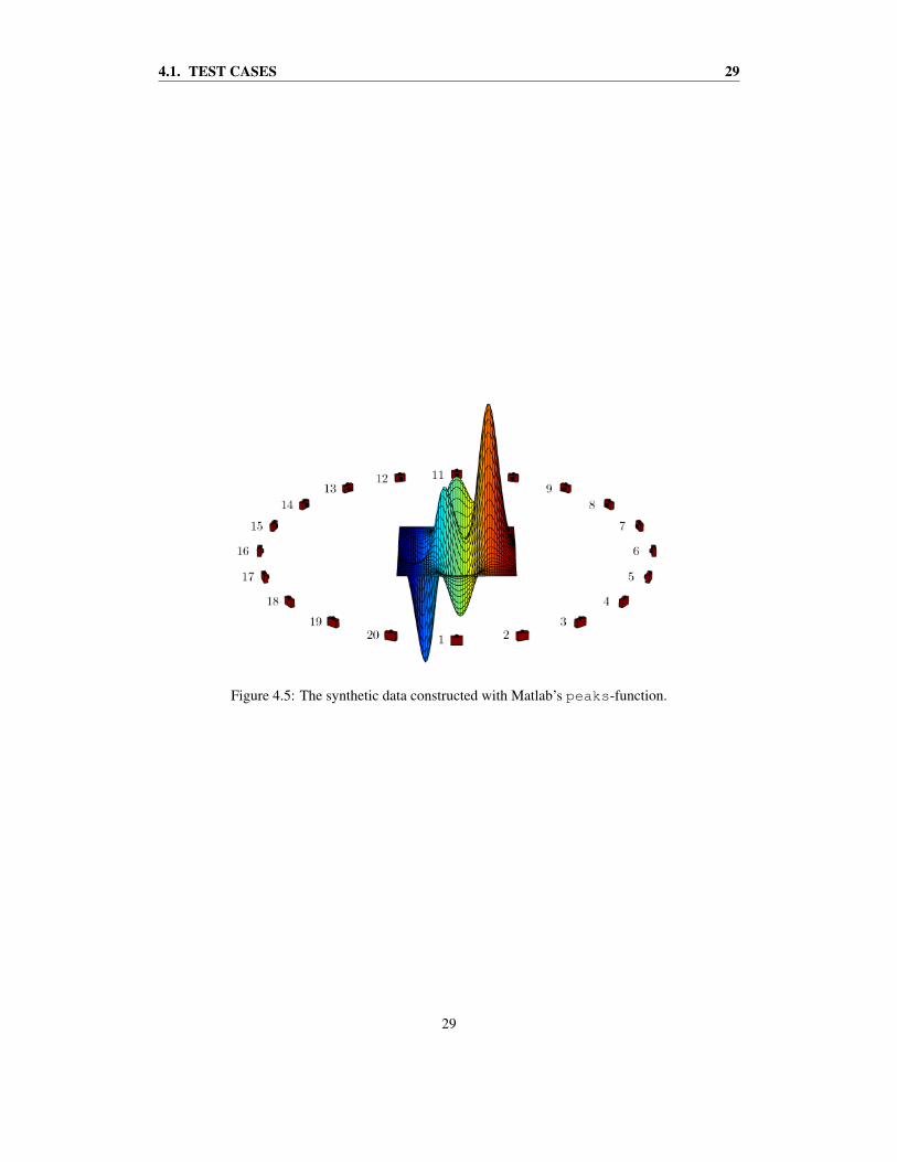
4.1.6 The synthetic dataThe synthetic data was constructed with Matlab’s peaks function. The cameras were aimed at theorigin and placed in a circle orbiting the data. See Figure 4.5. A total of 20 camera positions wereplaced, with a distance of 10 meters to the origin. The difference in yaw angle between every camerawas 18◦. This was a somewhat larger angular difference than in the real-world examples, which leadto the necessity of increasing the resolution parameter to 1 meter.

The entire synthetic point cloud consists of 5000 points. Though, to simulate occlusion culling,the half of the points that were farthest away from the camera, were removed from each view. Theroughly 2500 points of each view was used by the ICP in the search for relative transformations.

The 3D data in each view was perturbed by Gaussian noise to investigate the robustness of theregistration method. The estimated camera poses were compared with the actual ones, for noise lev-els with standard deviations σ = 0.01, 0.02, . . . , 0.10 meters. The mean errors in camera positionsand rotations was calculated for both the regular and the optimized case.

ICP was not used to obtain the very last relative transformation, T1,n. To be able to rightfullycompare the improvement of the optimization for different noise levels, the actual transformationwas used here.

28

4.1. TEST CASES 29

Figure 4.5: The synthetic data constructed with Matlab’s peaks-function.

29


30

Chapter 5

Results

5.1 Translation of the camera

The results from the translational experiment are shown in figures 5.1(a)–(c). In Figure 5.1(a) all theinitial guesses on the transformations were set to Tinitial = I4×4. The first camera in every figureis recognized by its slightly larger size.

By only looking at the cameras it can be hard to see just how bad the registrations went. Though,at a closer look, it is almost impossible to distinguish the desk, chair and the flower in the scene.The camera positions have been pushed closer to each other during the translation to the left. This isa consequence of this crude type of initial guess which needs the camera positions to be very closeto each other in order to make the correct registration. The registrations did improve on the wayback to the right. Camera positions were more tightly spaced on the way back due to the somewhatslower translation speed at that time.

The result when utilizing the other, more sophisticated initial guesses, Tinitial = Tprevious, isshown in Figure 5.1(b). The objects in the scene can now be distinguished, and as can be seen, thecamera almost returns to the starting point. It has deteriorated from its actual path mostly in they-direction.

Lastly, Figure 5.1(c) shows the optimized result, using the previous case as input. The loop hasbeen closed and the error has been spread among the transformations. Not much seems to havehappened to the scene. Though, by looking at the camera positions, it can be seen that they nowfollow a straighter path, as if the camera actually was moved along a rail.

The approximate cumulative translational error of the cameras y and z-positions is comparedbetween the regular case, and the optimized case in figures 5.2(a)–(b). In Figure 5.2(a), the errorin the y-direction increases faster than in the z-direction. Furthermore, the error in the y-directionincreases especially between camera positions 35-45.

In the optimized case, Figure 5.2(b), the cumulative error of the cameras’ y and z-positions hasbeen lowered.

The function values which are being minimized, equation 2.10, are given as output from fminconand are shown in Figure 5.3. The function value fluctuates strongly near the end, and in the searchfor a minimum fmincon disobeys the constraint to some extent. Though, in the end it finds areasonable minimum.

In the following cases, the plots showing the function being minimized, all have a somewhatsimilar look to them. Therefore this is the only one included.

31

32 CHAPTER 5. RESULTS

(a)

(b)

(c)

Figure 5.1: Translation of the camera aiming at an office desk. (a) Case with initial guessesTinitial = I4×4. (b) Regular case, with initial guesses Tinitial = Tprevious. (c) Optimized case.

32

5.1. TRANSLATION OF THE CAMERA 33

0 20 40 60 800

1

2

3

4

5

Camera position number

Cum

ulat

ive

tran

slat

iona

l err

or (

m)

Error in y−directionError in z−direction

(a)

0 20 40 60 800

1

2

3

4

5


Cum

ulat

ive

tran

slat

iona

l err

or (

m)

Error in y−directionError in z−direction

(b)

Figure 5.2: Approximative cumulative error in y and z-position of the camera. (a) Before optimiza-tion. (b) After optimization.

Figure 5.3: Values of the function being minimized, equation 2.10, during the optimization.

33


(a) (b)

Figure 5.4: The reconstructed room with chairs. (a) Before optimization. (b) After optimization.

5.2 Room with reference objects

The result of the registration of the room with reference objects is shown from above in figures5.4(a)–(b). The actual measures of the room are indicated by the dashed red rectangle.

The room roughly keeps its shape, though the accumulated error becomes visible at the end ofthe revolution, at the top wall. The topmost chair seems larger than the rest. This was during the firstfew frames where ICP had a hard time registering correctly. In this particular case every third framewas used in the registration. Different amounts of frames lead to different results. Using every thirdframe produced better results than using every second, or every fourth frame for example.

At the top right corner of the room, there is a gap with no points. This is a consequence ofthe glossy door situated at that position. The points on the door were removed by the confidencethreshold in the pre-filtering process.

As can be seen in Figure 5.4(b), the reconstructed room did not change much after the optimiza-tion.

A close-up was made on the camera positions, which can be seen in figures 5.5(a)–(b). Thecameras have been moved a little closer to each other in the optimized case. Furthermore, the firstcamera is now more to the center of the heap of cameras, though, this can be hard to see.

The cumulative translational error of the camera positions is shown for the regular case in Figure5.6(a), and for the optimized case in Figure 5.6(b). The translational error is kept about the same inthe z-direction, but is lowered in the x and y-directions.

5.3 Empty room

The result of the registration of the room without reference objects is shown in Figures 5.7(a)–(b).ICP has major problems when facing flat walls. When the corner finally appears in the range

34

5.3. EMPTY ROOM 35

(a) (b)

Figure 5.5: A close-up on the camera positions from the reconstructed room with chairs, where thefirst camera defines the coordinate axes. (a) Before optimization. (b) After optimization.

0 50 100 1500

5

10

15

20

25


Cum

ulat

ive

tran

slat

iona

l err

or (

m)

Error in x−directionError in y−directionError in z−direction

(a)

0 50 100 1500

5

10

15

20

25


Cum

ulat

ive

tran

slat

iona

l err

or (

m)

Error in x−directionError in y−directionError in z−direction

(b)

Figure 5.6: Approximative cumulative error in x, y and z-position of the camera. (a) Before opti-mization. (b) After optimization.

35


(a) (b)

Figure 5.7: The reconstructed empty room. (a) Before optimization. (b) After optimization.

images, the registration picks up momentum. Hence a small piece of the room turns out well. Theoptimization algorithm closes the loop, as can be seen in Figure 5.7(b), but it is not sufficient to givethe room its proper shape. This shows the importance of having reference objects of some sort forthis registration method to work.

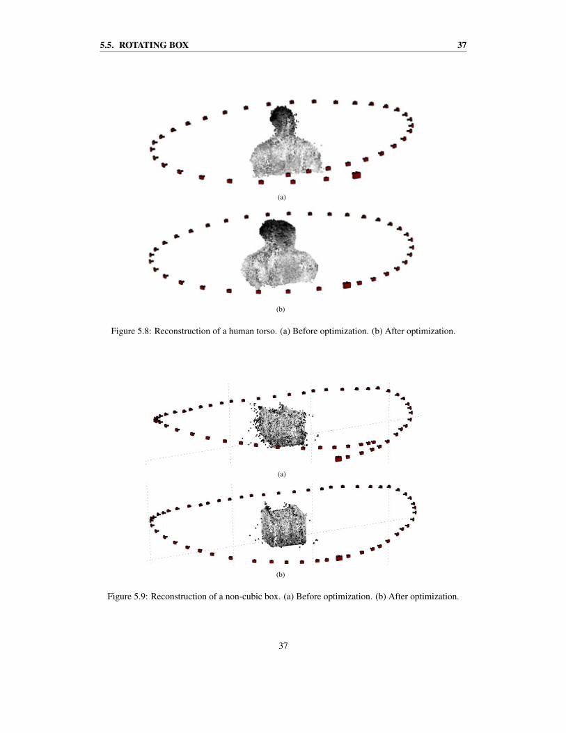
5.4 Rotating torsoThe result of the rotating torso case is shown in figures 5.8(a)–(b). The camera positions seem toorbit the torso in a nice-looking way, though, there is a slight overlap. The optimization algorithmremoves this overlap as can be seen in Figure 5.8(b).

Unfortunately, the camera positions seem to have been pushed out, away from the torso. Hencethe model, i.e. the author of this thesis, looks like he has gained some weight. The relative transfor-mations are the only thing which the optimization cares to preserve. It does not try to preserve thecameras distances to the object.

5.5 Rotating boxThe result of the rotating box registration is shown in figures 5.9(a)–(b). As in the previous case,the viewing angles of the cameras seem to have been corrected for after the optimization. In Figure5.10 the optimized box is shown from the top. The actual width of the box is shown in red and thewidth of the reconstructed box is shown in blue. Figure 5.10 shows that the angles of the box arevery close to accurate. Though, the box has expanded in every direction.

The white area in the middle of the box contains almost no points since the camera was aimingat the box from the side.

36

5.5. ROTATING BOX 37

(a)

(b)

Figure 5.8: Reconstruction of a human torso. (a) Before optimization. (b) After optimization.

(a)

(b)

Figure 5.9: Reconstruction of a non-cubic box. (a) Before optimization. (b) After optimization.

37


Figure 5.10: The optimized box from the top view. Comparison between actual measures (red), andmeasures from the reconstructed model (blue).

5.6 The synthetic data

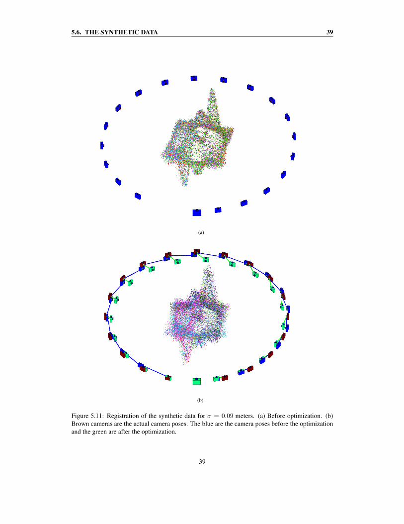
In Figure 5.11(a) an example of the performance of the sequential ICP is shown. Here, a Gaussianerror of σ = 0.09 meters has been applied to the data points. The second camera position, i.e.the first transformation, is not estimated very well since it was obtained through the initial guessTinitial = I4×4. The remaining relative transformations are more accurately estimated, thoughthere is a small error adding up, leaving a gap at the end. The model in the middle looks okaysince the cameras have kept a correct distance to the point clouds, and since only the first relativetransformation was very poorly estimated. In Figure 5.11(b) the actual camera positions, as well asthe camera positions after the optimization, have been put into the picture. The model in the middlehas now been put together using the optimized camera positions. During the process of closing theloop, the optimized camera positions have been pushed inwards, mainly at the far side. This leadsto a blurry point cloud in the center of the image.

By inspection of the length of the lines between the actual and the estimated camera poses inFigure 5.11(b), one can see that the overall error has been reduced after the optimization.

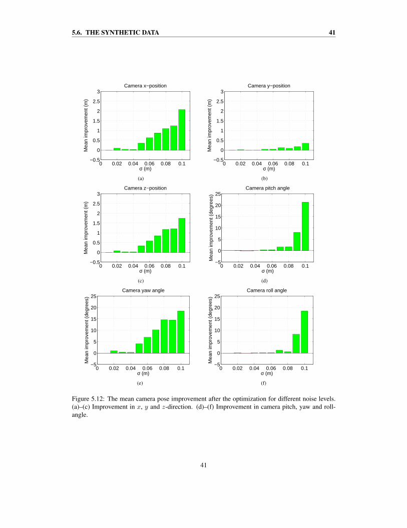
The mean improvements of the camera poses using the optimization algorithm over not usingit, are shown for different noise levels in figures 5.12(a)–(f). The success of the registration seemsto depend strongly on the amount of applied noise. ICP does well on its own if the applied noisehas a standard deviation below σ = 0.05 meters. For values higher than this, ICP obtains one ormore suboptimal relative transformations. In case of noise levels above σ = 0.05, the optimizationalgorithm improves the camera positions and their rotation angles.

The cameras’ y-positions are not altered very much, as expected. See Figure 5.12(b). The x andz-positions are improved about the same. Figure 5.12(a),(c). For every parameter the optimizationseem to do more good in case of more applied noise.

38

5.6. THE SYNTHETIC DATA 39

(a)

(b)

Figure 5.11: Registration of the synthetic data for σ = 0.09 meters. (a) Before optimization. (b)Brown cameras are the actual camera poses. The blue are the camera poses before the optimizationand the green are after the optimization.

39


For the cameras’ angles, the yaw-angle is most improved. This is also expected due to thegap that needed to be closed, see Figure 5.11(a). The pitch and roll-angles are only improvedsignificantly in the cases with high amounts of applied noise

40

5.6. THE SYNTHETIC DATA 41

0 0.02 0.04 0.06 0.08 0.1−0.5

0

0.5

1

1.5

2

2.5

3Camera x−position

Mea

n im

prov

emen

t (m

)

σ (m)

(a)

0 0.02 0.04 0.06 0.08 0.1−0.5

0

0.5

1

1.5

2

2.5

3Camera y−position

Mea

n im

prov

emen

t (m

)

σ (m)

(b)

0 0.02 0.04 0.06 0.08 0.1−0.5

0

0.5

1

1.5

2

2.5

3Camera z−position

Mea

n im

prov

emen

t (m

)

σ (m)

(c)

0 0.02 0.04 0.06 0.08 0.1−5

0

5

10

15

20

25Camera pitch angle

Mea

n im

prov

emen

t (de

gree

s)

σ (m)

(d)

0 0.02 0.04 0.06 0.08 0.1−5

0

5

10

15

20

25Camera yaw angle

Mea

n im

prov

emen

t (de

gree

s)

σ (m)

(e)

0 0.02 0.04 0.06 0.08 0.1−5

0

5

10

15

20

25Camera roll angle

Mea

n im

prov

emen

t (de

gree

s)

σ (m)

(f)

Figure 5.12: The mean camera pose improvement after the optimization for different noise levels.(a)–(c) Improvement in x, y and z-direction. (d)–(f) Improvement in camera pitch, yaw and roll-angle.

41


42

Chapter 6

Discussion

The success of registration depends on a myriad of parameters. Hence it is difficult to write code thattakes everything into account. Special cases though, are another matter. If one knows for examplehow fast the camera pans, at what sort of surfaces the camera is aimed or when a loop is supposed tooccur. Then the parameters could be given appropriate values, which will enhance the correctnessand attractiveness of the merged model.

As suspected, ICP has problems finding the optimal solution if for example the camera is pan-ning over a flat surface. This problem can be solved by giving the ICP a good initial guess on thetransformation. If the camera starts out at a position not facing a difficult area, the first transforma-tion can be assumed to be good. Consequently, that transformation can be used as an initial guess ofthe next transformation, and so on. This improved the attractiveness of the registrations quite a bit.

A reasonable question to ask would be: “Why didn’t you use SIFT to help with estimation ofcamera movement”? First of all, to compute the fundamental matrix used to estimate the cameramovement, at least seven corresponding points in two images are needed (Hartley and Zisserman,2003). It is important that these points are accurate. However, there is no certain way to automat-ically remove all blunders. If there are a few points which look the same in two images, there is ahigh likelihood of false matches. To reduce the number of false matches, one can let SIFT searchfor only large feature points. However, if the camera is aiming at homogeneous surfaces, SIFT canyield too few corresponding points to compute the fundamental matrix. Another problem with ToFcameras today, is their relatively small sensor. A higher resolution in the images would have givengreater accuracy when calculating the camera movement. Furthermore, the lens distortion in theamplitude images need to be corrected for. There was not enough time to implement this.

43

44 CHAPTER 6. DISCUSSION

44

Chapter 7

Conclusions

ToF cameras can indeed be used for constructing 3D models of objects and areas. However, duringmovement of the camera, or if objects in the scene move, the cameras still produce a lot of erroneouspoints. Therefore the filtering step is crucial for obtaining good end results.

ToF cameras are a bit more inaccurate than conventional laser scanners, but they are on thecontrary both quicker and cheaper. If a lower accuracy can be accepted, the ToF camera is a goodalternative for 3D reconstruction.

Considering that no odometry or any other method was used to obtain initial guesses on thetransformations in this thesis, the results can be seen as satisfactory. To obtain much better resultssuch methods need to be utilized. However, this will in many cases lead to increased computationtime.

The implemented optimization algorithm does its job, though, the results were not as good as wasinitially hoped for. The global camera positions and angles are improved, but no difference is madefor relative transformations that were more accurately determined than others. All transformationsare assumed to have the same amount of error in them. Hence, already well determined cameratransformations are often worsened.

45

46 CHAPTER 7. CONCLUSIONS

46

Chapter 8

Future work

The problem of reconstructing scenes in 3D can be split into two sub-problems. How to produceas accurate point clouds as possible, and how to present the data to the user in the best way? Thefirst thing that needs to be added in future work to improve the registration is some means of gettinginitial guesses on the transformations. A good solution is to attach odometry equipment to thecamera. Furthermore, if a conventional digital camera is attached to the ToF camera, methods forfinding and tracking features in a scene can also be used. Methods such as SIFT, SURF and FASTfor example. They can either be used on their own, or as a complement to the odometry data.

In this thesis, the grayscale amplitude images were used for coloring the 3D points. If a digitalcamera is added, the RGB colors could be assigned to the 3D points. Color would make it easier fora human to recognize objects and to navigate in a scene. Future work could also include attempts to,as automatically as possible, texture surfaces made from the point clouds. However, to adapt nicesurfaces to the data points, the point clouds need to be without any flying pixels. This would probablymean that the camera has to be standing still for a short period of time during the acquisition.

There are a few improvements that can be done connected to the ICP step. Different methodswork better in different situations. Some heuristics could be applied for the registration method toswitch to the most appropriate method in each view. In this thesis the point-to-point error was min-imized for instance, while the point-to-surface was suggested by Rusinkiewicz and Levoy (2001).This method was not thoroughly investigated since the data seemed too noisy in the beginning,yielding very uneven surfaces. Later a better filtering technique was employed, removing outliersby the help of a nearest neighbor search.

Since the point-to-point error metric was chosen, consecutively the closest points between modeland dataset were picked as corresponding points. Rusinkiewicz and Levoy (2001) propose a projec-tion based method, but this requires the point-to-surface error metric.

A random subsample of points was used for the ICP. This works well most of the time, butagainst surfaces with very little features, a subsample with a good distribution of normals wouldsurely work better.

It would be interesting to run the implemented code iteratively. To compute the sequential trans-formations, close the loop, and use the optimized camera positions to calculate new initial guesseson the relative transformations for the next iteration, and so on. A working loop detecting algorithmis also needed to take another step towards total automatization.

In this thesis the optimization method proposed by Castellani et al. (2002) was used. It tradesexactness for speed in some sense. Errors between points are not minimized, only the error betweencamera poses. No care is taken for transformations that were more accurately determined thanothers. Though, this can be difficult to verify. Furthermore, the convergence rate was perceived as

47

48 CHAPTER 8. FUTURE WORK

suspectedly slow. Perhaps some other way to represent angles than quaternions would increase theconvergence rate, e.g. direction cosine matrices. However, there are many alternative optimizationalgorithms that perhaps would perform better. The method described in Borrmann et al. (2008) andSprickerhof et al. (2009) seems very interesting. Moreover there are many ongoing open sourceprojects available online1. Some of these would be interesting to test with ToF camera data as input.

1www.openslam.org

48

References

Akca, D. (2007). Matching of 3d surfaces and their intensities. ISPRS J Photogramm, 62(2):112 –121.

Akca, D. and Gruen, A. (2007). Generalized least squares multiple 3d surface matching. In-ternational Archives of Photogrammetry, Remote Sensing, and Spatial Information Sciences,XXXVI(3/W52):1–7.

Almhdie, A., Leger, C., Deriche, M., and Ledee, R. (2007). 3d registration using a new imple-mentation of the icp algorithm based on a comprehensive lookup matrix: Application to medicalimaging. Pattern Recogn. Lett., 28(12):1523–1533.

Artner, P. (2009). Globally consistent registration of time-of-flight camera images. Master’s thesis,Faculty of Technology, Bielefeld University.

Arun, K. S., Huang, T. S., and Blodstein, S. D. (1987). Least-squares fitting of two 3-d point sets.IEEE T Pattern Anal, 9(5):698–700.

Bae, K.-H. and Lichti, D. D. (2008). A method for automated registration of unorganised pointclouds. ISPRS J Photogramm, 63(1):36 – 54.

Barnea, S. and Filin, S. (2008). Keypoint based autonomous registration of terrestrial laser point-clouds. ISPRS J Photogramm, 63(1):19 – 35.

Bergevin, R., Soucy, M., Gagnon, H., and Laurendeau, D. (1996). Towards a general multi-viewregistration technique. IEEE Transactions on Pattern Analysis and Machine Intelligence, 18:540–547.

Besl, P. J. and McKay, N. D. (1992). A method for registration of 3-d shapes. IEEE T Pattern Anal,14(2):239–256.

Borrmann, D., Elseberg, J., Lingemann, K., Nuchter, A., and Hertzberg, J. (2008). Globally consis-tent 3d mapping with scan matching. Robot. Auton. Syst., 56(2):130–142.

Bostrom, G., Goncalves, J. G., and Sequeira, V. (2008). Controlled 3d data fusion using error-bounds. ISPRS J Photogramm, 63(1):55 – 67.

Castellani, U., Fusiello, A., and Murino, V. (2002). Registration of multiple acoustic range viewsfor underwater scene reconstruction. Computer Vision and Image Understanding, 87:78–89.

Chen, Y. and Medioni, G. (1992). Object modelling by registration of multiple range images. ImageVision Comput., 10(3):145–155.

49

50 REFERENCES

Chetverikov, D., Stepanov, D., and Krsek, P. (2005). Robust euclidean alignment of 3d point sets:the trimmed iterative closest point algorithm. Image Vision Comput., 23(3):299–309.

Fischler, M. A. and Bolles, R. C. (1981). Random sample consensus: A paradigm for model fittingwith applications to image analysis and automated cartography. Comm ACM, 24(6):381–395.

Fors Nilsson, H. and Grundberg, D. (2009). Plane-based close range photogrammetric reconstruc-tion of buildings. Master’s thesis, Department of Computing Science, Umea University.

Fuchs, S. and Hirzinger, G. (2008). Extrinsic and depth calibration of tof-cameras. In CVPR.

Fusiello, A., Castellani, U., Ronchetti, L., and Murino, V. (2002). Model acquisition by registrationof multiple acoustic range views. In ECCV ’02: Proceedings of the 7th European Conference onComputer Vision-Part II, pages 805–822, London, UK. Springer-Verlag.

Godin, G., Rioux, M., and Baribeau, R. (1994). Three-dimensional registration using range andintensity information. In El-Hakim, S. F., editor, Videometrics III, volume 2350, pages 279–290.SPIE.

Gruen, A. and Akca, D. (2005). Least squares 3d surface and curve matching. ISPRS J Photogramm,59(3):151 – 174.

Hartley, R. I. and Zisserman, A. (2003). Multiple View Geometry in Computer Vision. CambridgeUniversity Press, ISBN: 0521540518, 2nd edition.

Laser Scanner Survey 2005 (2005). 3D Laser Scanner Hardware Sur-vey. http://www.pobonline.com/POB/Protected/Files/PDF/POB0105-LaserScanningSurvey.pdf, last visited 2010-02-20.

Lowe, D. G. (1999). Object recognition from local scale-invariant features. In Proc Intl Conf onComputer Vision, pages 1150–1157, Corfu, Greece.

Lowe, D. G. (2004). Distinctive image features from scale-invariant keypoints. Int J Comp Vis,60(2):91–110.

Lu, F. and Milios, E. (1997). Globally consistent range scan alignment for environment mapping.Autonomous Robots, 4:333–349.

Magnusson, M. (2006). 3D Scan Matching for Mobile Robots with Application to Mine Mapping.PhD thesis, Licentiate thesis, Orebro University.

May, S., Fuchs, S., Droschel, D., Holz, D., and Nuchter, A. (2009). Robust 3d-mapping with time-of-fligt cameras. In IROS. http://www.ais.uni-bonn.de/˜holz/papers/may_2009_iros_slides.pdf and http://www.ais.uni-bonn.de/˜holz/papers/may_2009_iros.pdf, last visited 2010-02-20.

Mian, A. S., Bennamoun, M., and Owens, R. (2006). Three-dimensional model-based object recog-nition and segmentation in cluttered scenes. IEEE Transactions on Pattern Analysis and MachineIntelligence, 28:1584–1601.

Moore, A. (1991). An introductory tutorial on kd-trees. Technical report, Computer Laboratory,University of Cambridge, Pittsburgh, PA.

Mure Dubois, J. and Hugli, H. (2008). Fusion of time of flight camera point clouds. In Workshopson Multi-camera and Multi-modal Sensor Fusion Algorithms and Applications - M2SFA2, pagesxx–yy.

50

REFERENCES 51

Nordqvist, M. (2010). Creation and evaluation of different algorithms for extraction of depth infor-mation from a time of flight 3d camera. Master’s thesis, Umea universitet.

Nuchter, A., Lingemann, K., Hertzberg, J., and Surmann, H. (2007). 6d slam—3d mapping outdoorenvironments: Research articles. J. Field Robot., 24(8-9):699–722.

Olson, E. (2008). Robust and Efficient Robotic Mapping. PhD thesis, Massachusetts Institute ofTechnology, Cambridge, MA, USA.

Pottmann, H., Leopoldseder, S., and Hofer, M. (2004). Registration without icp. Computer Visionand Image Understanding, 95(1):54–71.

Prusak, A., Schiller, I., Melnychuk, O., Koch, R., and Roth, H. (2008). Pose estimation and mapbuilding with a pmd-camera for robot navigation. International Journal of Intelligent SystemsTechnologies and Applications, 5(Issue on Dynamic 3D Imaging):355–364.

Pulli, K. (1999). Multiview registration for large data sets. In 3DIM, pages 160–168.

Ronnholm, P., Honkavaara, E., Erving, A., Nuikka, M., Haggren, H., Kaasalainen, S., Hyyppa, H.,and Hyyppa, J. (2008). Registration of airborne laser scanning point clouds with aerial imagesthrough terrestrial image blocks. In ISPRS08, page B1: 473 ff.

Rusinkiewicz, S. and Levoy, M. (2001). Efficient variants of the icp algorithm. 3D Digital Imagingand Modeling, International Conference on, 0:145.

Soderkvist, I. and Wedin, P. (1994). On condition numbers and algorithms for determining a rigidbody movement. BIT, 34:424–436.

Sharp, G. C., Lee, S. W., and Wehe, D. K. (2000). Icp registration using invariant features.

Smith, E. R., King, B. J., Stewart, C. V., and Radke, R. J. (2008). Registration of combined range-intensity scans: Initialization through verification. Comp Vis Imag Under, 110(2):226 – 244.

Sprickerhof, J., Nuchter, A., Lingemann, K., and Hertzberg, J. (2009). An explicit loop closingtechnique for 6D SLAM. In In Proceedings of the 4th European Conference on Mobile Robots(ECMR ’09), Mlini/Dubrovnic, Croatia.

SR4000 Manual (2009). SwissRanger SR4000 User Manual v1.3. http://www.mesa-imaging.ch/customer/Customer_CD/SR4000_Manual.pdf, last visited2010-02-18.

The Matrix and Quaternions FAQ (2003). Version 1.21. http://www.j3d.org/matrix_faq/matrfaq_latest.html, last visited 2010-06-15.

Thrun, S. and Montemerlo, M. (2005). The GraphSLAM algorithm with applications to large-scalemapping of urban structures. International Journal on Robotics Research, 25(5/6):403–430.

Wheeler, M. and Ikeuchi, K. (1995). Iterative estimation of rotation and translation using the quater-nion. Technical Report CMU-CS-95-215, Computer Science Department, Pittsburgh, PA.

Wiklund, A. (2006). Registration approaches for noisy 3D data representing natural scenes. Master’sthesis, Lulea Tekniska Universitet.

Williams, J. and Bennamoun, M. (2001). Simultaneous registration of multiple corresponding pointsets. Comput. Vis. Image Underst., 81(1):117–142.

51

Documents

Registration of multiple ToF camera point clouds327071/FULLTEXT01.pdf · Registration of multiple ToF camera point clouds Tobias Hedlund ... Chetverikov et al. (2005) proposed a version