FI;aHEWLETT.:~ PACKARD

Register Allocation for ModuloScheduled Loops: Strategies,Algorithms and Heuristics

B. R. Rau, M. Lee, P. P. Tirumalai, M. S. SchlanskerComputer Systems LaboratoryHPL-92-48April, 1992

register allocation,modulo scheduling,software pipelining,instructionscheduling, codegeneration,instruction-levelparallelism,multiple operationissue, VLIWprocessors, "eryLong Instructionword processors

Software pipelining is an important instructionscheduling technique for efficiently overlappingsuccessive iterations of loops and executing them inparallel. This technical report studies the task ofregister allocation for software pipelined loops, bothwith and without hardware features that arespecifically aimed at supporting software pipelines.Register allocation for software pipelines presentscertain novel problems leading to unconventionalsolutions, especially in the presence of hardwaresupport. This technical report formulates these novelproblems and presents a number of alternativesolution strategies. These alternatives arecomprehensively tested against over one thousandloops to determine the best register allocationstrategy, both with and without the hardwaresupport for software pipelining.

To be published in an abridged form, as "Register Allocation for Software Pipelined Loops", in theProceedings of the ACMSIGPLAN '92 Conference on Programming Language Design andImplementation, San Francisco, June 1992

© Copyright Hewlett-Packard Company 1992

Internal Accession Date Only

1 Introduction

1.1 Software pipelining

Software pipelining [1] is a loop scheduling technique which yields highly optimized loopschedules. Algorithms for achieving software pipelining fall into two broad classes:

• modulo scheduling as formulated by Rau and Glaeser [2] and,

• algorithms in which the loop is continuously unrolled and scheduled until a situation isreached which allows the schedule to wrap back on itself without draining the pipelines [3].

Although, to the best of our knowledge, there have been no published measurements on this issue, itis our belief that the second class of software pipelining algorithms can cause unacceptably largecode size expansion. Consequently, our interest is in modulo scheduling. In general, this is an NP­complete problem and subsequent work has focused on various heuristic strategies for performingmodulo scheduling ([4-7] and the as yet unpublished heuristics in the Cydra 5 compiler [8]).Modulo scheduling of loops with early exits is described by Tirumalai, et al. [9]. Moduloscheduling is applicable to RISC, CISC, superscalar, superpipelined, and VLIW processors, and isuseful whenever a processor implementation has parallelism either by virtue of having pipelinedoperations or by allowing multiple operations to be issued per cycle.

This technical report describes methods for register allocation of modulo scheduled loops that weredeveloped at Cydrome over the period 1984-1988, but which have not as yet been published. Thesetechniques are applicable to VLIW processors such as the Cydra 5 [10]. The processor modelsupports the initiation of multiple operations in a single cycle where each operation may havelatency greater than one cycle. The use of hardware features, that specifically support the efficientexecution of modulo scheduled loops, is assumed. In addition to the conventional general-purposeregister file (GPR), these features include rotating register files (register files supporting compiler­managed hardware renaming, which were termed the MultiConnect in the Cydra 5), predicatedexecution, and the Iteration Control Register (ICR) file (a boolean register file that holds thepredicates) [8, 10]. This technical report also considers the register allocation of modulo scheduledloops on processors that have no special support for modulo scheduling.

Our discussion is limited to register allocation following modulo scheduling. Register allocationprior to modulo scheduling would place unacceptable constraints on the schedule and would,therefore, result in poor performance. Concurrent scheduling and register allocation is preferable,but how this is to be achieved, in the context of modulo scheduling, is not understood. Thistechnical report does not attempt to describe a complete scheduling-allocation strategy. For instance,little will be said on the important issue of what to do if the number of registers required by theregister allocation exceeds the number available. Instead, the focus is on studying the relativeperformance of various allocation algorithms with respect to the number of registers that they endup using and their computational complexity.

In the rest of this section, we provide a brief overview of certain terms associated with moduloscheduling, descriptions of predicated execution and rotating register files, and of moduloscheduled code structure in the presence of this hardware support. We also examine the nature ofthe lifetimes that the register allocator must deal with for modulo scheduled loops. Section 2discusses the various register allocation strategies and code schemas that can be employed, and the

1

interdependencies between them. In the context of these alternatives, the register allocation problemis formulated in Section 3 and the candidate register allocation algorithms are laid out in Section 4.Section 5 describes the experiments performed and examines the data gathered from thoseexperiments. Section 6 places this work in a broader perspective and, finally, Section 7 states ourconclusions.

1.2 A quick overview of modulo scheduling

A rotating register file is addressed by adding the register specifier in the instruction to thecontents of the Iteration Control Pointer (ICP) modulo the number of registers in the rotatingregister file. A special loop control operation, brtop, decrements the ICP amongst other actions. Asa result of the brtop operation, a register that was previously specified as ri would have to bespecified as ri+l> and a different register now corresponds to the specifier rio This allows the lifetimeof a value generated by an operation in one iteration to co-exist with the corresponding valuesgenerated in previous and subsequent iterations. Newly generated values are written to successivelocations in the rotating register file and do not overwrite previously generated values even thoughexactly the same code is being executed repeatedly. This also introduces the need for the compilerto perform value tracking; the same value, each time it is used, may have to be referred to by adifferent register specifier depending on the number of brtop operations that lie between that useand the definition [8].

The Iteration Control Register file, ICR, is a rotating register file that stores boolean values calledpredicates. Predicated execution allows an operation to be conditionally executed based on thevalue of the predicate associated with it. Each predicated operation has an additional registerspecifier that specifies a register in the predicate register file. For example, the operation

a =op(b,c) if Pi

executes if the predicate Pi is one, and is nullified if Pi is zero. The primary motivation forpredicated execution is to achieve effective modulo scheduling of loops containing conditionalbranches [8, 10]. Predicates permit the if-conversion [11] of the loop body, thereby eliminating allbranches from the loop body. The resulting branch-free loop body can now be modulo scheduled.In the absence of predicated execution, other techniques must be used which require either multipleversions of code corresponding to the various combinations of branch conditions [12, 3] orrestrictions on the extent of overlap between successive iterations [5]. A secondary benefit ofpredicated execution, the one relevant to this study, is in controlling the filling and draining of thesoftware pipeline in a highly compact form of modulo scheduled code known as kernel-only code.

The number of cycles between the initiation of successive iterations in a modulo schedule is termedthe initiation interval (II). The schedule for an iteration can be divided into stages consisting ofII cycles each. The number of stages in one iteration is termed the stage count (SC). If theschedule length is SL cycles, the number of stages is given by

SC =r~tl.

Figure 1 shows the record of execution of five iterations of the modulo scheduled loop with a stagecount of 4. The execution of the loop can be divided into three phases: ramp up, steady state, andramp down. In Figure 1, the first 3*11 cycles, when not all stages of the software pipeline execute,

2

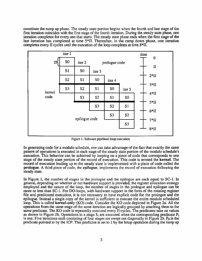
constitute the ramp up phase. The steady state portion begins when the fourth and last stage of thefirst iteration coincides with the first stage of the fourth iteration. During the steady state phase, oneiteration completes for every one that starts. The steady state phase ends when the first stage of thelast iteration has completed at time 5*11. Thereafter, in the ramp down phase, one iterationcompletes every II cycles until the execution of the loop completes at time 8*11.

time0

II

2*11

3*11

4*11

5*11

6*11

7*11

8*11

{ SO iter 2 prologue code

Sl SO iter 3

S2 Sl SO iter 4

S3 S2 SI SO iter 5

S3 S2 SI SO

S3 S2 SI

S3 S2epilogue code

S3

kernelcode

iter 1

II

Figure 1. Software pipelined loopexecution

In generating code for a modulo schedule, one can take advantage of the fact that exactly the samepattern of operations is executed in each stage of the steady state portion of the modulo schedule'sexecution. This behavior can be achieved by looping on a piece of code that corresponds to onestage of the steady state portion of the record of execution. This code is termed the kernel. Therecord of execution leading up to the steady state is implemented with a piece of code called theprologue. A third piece of code, the epilogue, implements the record of execution following thesteady state.

In Figure 1, the number of stages in the prologue and the epilogue are each equal to SC-l. Ingeneral, depending on whether or not hardware support is provided, the register allocation strategyemployed and the nature of the loop, the number of stages in the prologue and epilogue can bemore or less than SC-l. For DO-loops, with hardware support in the form of the rotating registerfile and predicated execution, it is not necessary to have explicit code for the prologue and theepilogue. Instead a single copy of the kernel is sufficient to execute the entire modulo scheduledloop. This is called kernel-only (KO) code. Consider the KO code depicted in Figure 2a. All theoperations from the same stage of the same iteration are logically grouped by attaching them to thesame predicate. The KO code is repeatedly executed every II cycles. The predicates take on valuesas shown in Figure 2b. Operations in a stage S, are executed when the corresponding predicate Piis one. Five iterations each consisting of four stages are swept out diagonally in Figure 2b. Po is thepredicate pointed to by the ICP. This predicate is set to 1 by the brtop operation during the ramp up

3

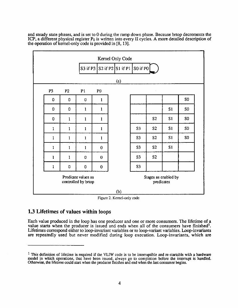
and steady state phases, and is set to 0 during the ramp down phase. Because brtop decrements theICP, a different physical register Po is written into every II cycles. A more detailed description ofthe operation of kernel-only code is provided in [8, 13].

Kernel Only Code

IS3 ifP31 S2 if P21Sl ifPll SOif pol:)(a)

P3 P2 PI PO

0 0 0 1 SO

0 0 1 1 SI SO

0 1 1 1 S2 SI SO

1 1 1 1 83 82 81 SO

1 1 1 1 83 S2 81 80

1 1 1 0 83 82 81

1 1 0 0 83 S2

1 0 0 0 83

Predicatevaluesas Stagesas enabledbycontrolledby brtop predicates

(b)

Figure 2. Kernel-only code

1.3 Lifetimes of values within loops

Each value produced in the loop has one producer and one or more consumers. The lifetime of avalue starts when the producer is issued and ends when all of the consumers have finished'.Lifetimes correspond either to loop-invariant variables or to loop-variant variables. Loop-invariantsare repeatedly used but never modified during loop execution. Loop-invariants, which are

1 This definition of lifetime is required if the VLIW code is to be interruptible and re-startable with a hardwaremodel in which operations, that have been issued, always go to completion before the interrupt is handled.Otherwise, thelifetime could startwhen theproducer finishes andend when thelastconsumer begins.

4

referenced in the loop, are assumed to have already been allocated in the (non-rotating) GPR fileusing conventional register allocation techniques. This is not the topic of this technical report.

A new value is generated in each iteration for a loop-variant and, consequently, there is a differentlifetime corresponding to each iteration. Loop-variants can be further categorized based on whetheror not the value defined in one iteration is used in a subsequent one, and on whether or not a valuedefined in one of the last few iterations is used after the loop. That a loop-variant is used by asubsequent iteration is equivalent to saying that each iteration uses a value defined by a previousiteration. In the case of the first few iterations, these previous iterations do not exist, and theexpected values must be generated before the loop is entered and, therefore, are live-in to the loop.Likewise, if a value that is defined in one of the last few iterations is used after the loop, it will belive-out from the loop.

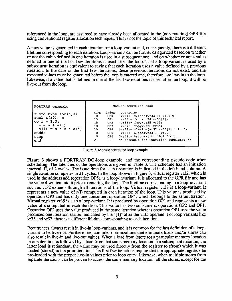
FORTRAN example Modulo scheduled code

subroutine foo(a,s)real a(10), sdo i = 1,35

s = s + a (i)a(i) = s * s * a(i)

enddostopend

time indexo OPO

13 OPI15 OP218 OP320 OP4OOPSo OP6

21

operationvr34:- m2read(vr33[1] lit: 0)vr35:- fadd(vr34 vr35[1])vr36:- fmpy(vr35 vr35)vr37:- fmpy(vr36 vr34)

$vr38:- m1write(vr37 vr33[1] lit: 0)vr33:- a1add(vr33[lj vr32)

$vr39:- brtop(slit: 'L.4-foo')** schedule for iteration completes **

Figure3. Modulo scheduled loopexample

Figure 3 shows a FORTRAN DO-loop example, and the corresponding pseudo-code afterscheduling. The latencies of the operations are given in Table 3. The schedule has an initiationinterval, II, of 2 cycles. The issue time for each operation is indicated in the left hand column. Asingle iteration completes in 21 cycles. In the loop shown in Figure 3, virtual register vr32, which isused in the address add (operation OP5), is a loop-invariant. It is allocated to the GPR file and hasthe value 4 written into it prior to entering the loop. The lifetime corresponding to a loop-invariantsuch as vr32 extends through all iterations of the loop. Virtual register vr37 is a loop-variant. Itrepresents a new value of a(i) computed in each iteration of the loop. This value is produced byoperation OP3 and has only one consumer, operation OP4, which belongs to the same iteration.Virtual register vr35 is also a loop-variant. It is produced by operation OPI and represents a newvalue of s computed in each iteration. This value has two consumers, operations OP2 and OPI.Operation on uses the value produced in the same iteration whereas operation OPI uses the valueproduced one iteration earlier, indicated by the "[I]" after the vr35 operand. For loop variants likevr35 and vr37, there is a different lifetime corresponding to each iteration.

Recurrences always result in live-in loop-variants, and it is common for the last definition of a loop­variant to be live-out. Furthermore, compiler optimizations that eliminate loads and/or stores canalso result in live-in and live-out values. When a load from (store to) a particular memory locationin one iteration is followed by a load from that same memory location in a subsequent iteration, thelatter load is redundant; the value may be used directly from the register to (from) which it wasloaded (stored) in the prior iteration. The first few iterations require that the appropriate registers bepre-loaded with the proper live-in values prior to loop entry. Likewise, when multiple stores fromseparate iterations can be proven to access the same memory location, all the stores, except for the

5

last one, are redundant and can be eliminated. This assumes that that last store actually occurs. Inthe case of the last few iterations, the supposedly redundant store, that was supposed to be coveredby a store in a subsequent iteration, is, in fact, not redundant since the iteration containing thecovering store is not executed. The last value that should have been stored must be stored afterexiting the loop and, so, must be live-out. Such load-store optimizations, of scalar as well assubscripted references, were performed by the Cydra 5 compiler [8, 14] and have also been studiedby Callahan, et al. [15].

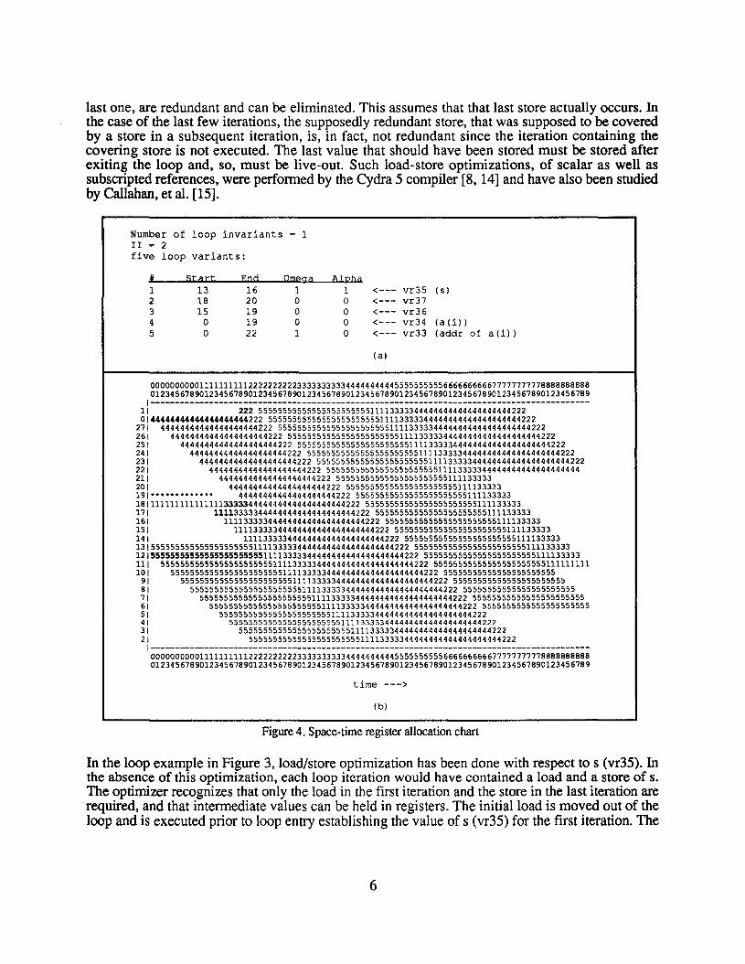
Number of loop invariants 1II = 2five loop variants:

It Start End Omega Alpha1 13 16 1 1 <--- vr35 (s)2 18 20 0 0 <--- vr373 15 19 0 0 <--- vr364 0 19 0 0 <--- vr34 (a (i))5 0 22 1 0 <--- vr33 (addr of a (L)

(a)

000000000011111111112222222222333333333344444444445555555555666666666677777777778888888888012345678901234567890123456789012345678901234567890123456789012345678901234567890123456789

1------------------------------------------------------------------------------------------11 222 55555555555555555555555111133333444444444444444444442220144444444444444444444222 5555555555555555555555511113333344444444444444444444222

271 44444444444444444444222 5555555555555555555555511113333344444444444444444444222261 44444444444444444444222 5555555555555555555555511113333344444444444444444444222251 44444444444444444444222 5555555555555555555555511113333344444444444444444444222241 44444444444444444444222 5555555555555555555555511113333344444444444444444444222231 44444444444444444444222 5555555555555555555555511113333344444444444444444444222221 44444444444444444444222 5555555555555555555555511113333344444444444444444444211 44444444444444444444222 55555555555555555555555111133333201 44444444444444444444222 55555555555555555555555111133333191············· 44444444444444444444222 555555555555555555555551111333331811111111111111113333344444444444444444444222 55555555555555555555555111133333171 11113333344444444444444444444222 55555555555555555555555111133333161 11113333344444444444444444444222 55555555555555555555555111133333151 11113333344444444444444444444222 55555555555555555555555111133333141 11113333344444444444444444444222 5555555555555555555555511113333313155555555555555555555511113333344444444444444444444222 555555555555555555555551111333331215555555555555555555555511113333344444444444444444444222 55555555555555555555555111133333111 5555555555555555555555511113333344444444444444444444222 55555555555555555555555111111111101 5555555555555555555555511113333344444444444444444444222 55555555555555555555555

91 5555555555555555555555511113333344444444444444444444222 5555555555555555555555581 5555555555555555555555511113333344444444444444444444222 5555555555555555555555571 5555555555555555555555511113333344444444444444444444222 5555555555555555555555561 5555555555555555555555511113333344444444444444444444222 555555555555555555555551 555555555555555555555551111333334444444444444444444422241 555555555555555555555551111333334444444444444444444422231 555555555555555555555551111333334444444444444444444422221 55555555555555555555555111133333444444444444444444442221------------------------------------------------------------------------------------------000000000011111111112222222222333333333344444444445555555555666666666677777777778888888888012345678901234567890123456789012345678901234567890123456789012345678901234567890123456789

time --->

(b)

Figure4. Space-time register allocation chart

In the loop example in Figure 3, load/store optimization has been done with respect to s (vr35). Inthe absence of this optimization, each loop iteration would have contained a load and a store of s.The optimizer recognizes that only the load in the first iteration and the store in the last iteration arerequired, and that intermediate values can be held in registers. The initial load is moved out of theloop and is executed prior to loop entry establishing the value of s (vr35) for the first iteration. The

6

initial value is, therefore, live-in to the loop. Subsequent iterations use the values generated oneiteration earlier (vr35[1]). Correspondingly, the store in the last iteration is moved out of the loopand is executed after loop exit. The value of s calculated in the last iteration is required by this storeand, therefore, must be live-out.

After optimization and scheduling, the set of lifetimes corresponding to a single loop-variant ispresented to the register allocator as a 4-tuple. Each 4-tuple is of the form (start, end, omega, alpha).The parameters start and end specify, respectively, the issue time of the producer of a value and thelatest completion time amongst all the operations that consume that value. Both start and end areexpressed relative to the initiation time of the iteration containing the producer. Omega is one lessthan the highest numbered iteration that uses the value defined by the first iteration, i.e., it is thenumber of iterations spanned by that value. It is also the number of live-in values for the loop­variant. Alpha specifies the number (counting back) of iterations from the end of the loop in whichthe earliest live-out value was defined. It is also the number of live-out values for the loop variant.For instance, if alpha =1, the only live-out value was defined in the last iteration; if alpha =2, thevalues of the loop variant defined in the last two iterations are both live-out. Even if we want only thevalue from the second last iteration (and not that from the last iteration), we define alpha to be 2.

The example in Figure 3 has five loop-variants which are shown in Figure 4a. The first and the fifthhave an omega = 1 indicating that there is one live-in value for each. The live-in value for loop­variant 1 is the initial value of s, and that for loop-variant 5 is the initial address of a(i), i.e., theaddress of a(I). These two values must be pre-loaded into the appropriate registers prior to loopentry. Loop-variant 1 also has an alpha =1 indicating that the value computed in the last iteration islive-out. This is the final value of s which must be stored after loop exit.

Figure 4b shows a space-time diagram generated by the register allocator for the 35 iterations of theexample in Figure 3. The horizontal axis represents time in clock cycles advancing from the far left(cycle 0) to the far right (cycle 89). The vertical axis denotes physical register space. The number ofrows in the chart indicates the number of registers used in the achieved allocation. Once a value isgenerated into a physical register ri, it occupies that register until the lifetime ends. The same loop­variant produced in the next iteration is generated into physical register ri-l due to the decrementingof the ICP (even though the register specifier used is the same). If ri is 0, ri-l will be the highestnumbered register. As iterations are initiated every II cycles, the start times of these two lifetimes areII cycles apart. This gives rise to the wand portion (the diagonal band) of the set of lifetimes for aloop-variant as each iteration yields a lifetime which is lower by one register and to the right by IIcycles from the lifetime in the previous iteration. The lifetime generated by the first iteration isshown in boldface. Live-in values, which are pre-loaded prior to loop entry, must remain in theregisters until their lifetimes end. This adds a leading blade to the wand of recurring values whichextends, on the left, all the way through cycle O. For example, the leading blade for loop-variant 1occupies register 18 from cycle 0 to cycle 14. Note that the blade lifetime need not always be longerthan the wand lifetime. For instance, the leading blade for loop-variant 5, which occupies register 13,is shorter than the lifetime for the first iteration, which is in register 12. This is because start is lessthan II for this loop-variant. As discussed, the lifetimes of live-out values, which are used after loopexit, must be extended until the loop completes. This adds a trailing blade to the wand ofrecurring values. For example, the trailing blade for loop-variant 1 occupies register 11 from cycles85 through 89. The thicknesses of the leading and trailing blades depend on the values of omegaand alpha, respectively. For example, if loop-variant 1 had omega =2, the leading blade wouldinclude register 19.from cycles 0 through 12 as indicated by the asterisks in Figure 4b.

7

When the possibility for confusion is present, we shall refer to a single lifetime (single live range)as a scalar lifetime and to the set of lifetimes corresponding to a loop-variant, across the entireexecution of the loop, as a vector lifetime. The register allocation problem involves packing thesevector lifetimes (wands with or without leading or trailing blades) as tightly as possible in the space­time plane.

2 Code Generation Strategies

For our purposes here, three activities are involved in generating code for modulo scheduled loops:modulo scheduling, register allocation and determining the correct code schema to use. Registerallocation is the topic of this technical report. However, the manner in which this is done dependsboth on the presence or absence of rotating register files as well as the code schema used. Any codeschema can be assembled from the following components, for each of which the correspondingnotation is also listed:

• prologue code (P),

• kernel code (K),

• unrolled kernel code (K"),

• epilogue code (E),

• multiple-epilogue code (En),• a sequential, preconditioning loop (S).

For instance, a specific code schema consisting of a prologue, an unrolled kernel, and multipleepilogues would be denoted by (PKnEn) whereas one with a preconditioning loop, a prologue,unrolled kernel, and epilogue would be denoted by (SPKnE). In the special case when the codeschema consists of only the kernel or unrolled kernel code, we add the suffix 0 (KO, J(ll0). Wehave two schemes for handling the overlapping lifetimes for a loop-variant that are encountered inmodulo scheduled code:

• static renaming via modulo variable expansion, (MVE), and• dynamic remapping via the use of rotating register files (DR).

Lastly, we shall consider two styles of register allocation:

• blades allocation, (BA), and

• wands-only allocation (WO).

All of these are elaborated upon below. The code schema, the renaming scheme and the style ofregister allocation cannot be selected independently. For instance, wands-only allocation precludeskernel-only code and vice versa, whereas blades allocation is compatible with both the kernel-onlyschema as well as the PKE schema. Modulo variable expansion always requires kernel unrolling.Furthermore, the choice of code schema is influenced and limited by the nature of the loop (00­loop or WHILE-loop) and whether predicated execution or rotating register files or both are present[13].

A register allocation strategy is a specific combination of the register allocation style, renamingscheme and code schema. Table 1 lists the legal register allocation strategies for all combinations of

8

the loop type and the hardware support provided. In this technical report, we shall only discuss indetail DO-loops with either no hardware support or with both predicated execution and rotatingregister files. Consequently, there are three register allocation strategies that we shall examine indetail:

• KO/DR/BA,• PKEn/DR/WO, and

• PKnEn/MVE/WO or SPKnE/MVE/WO.

When there is no risk of confusion, we shall abbreviate and refer to the first two strategies as theBA and WO strategies, respectively, and to both versions of the third one, collectively, as the MVEstrategy.

2.1 Code generation with hardware support for modulo scheduling

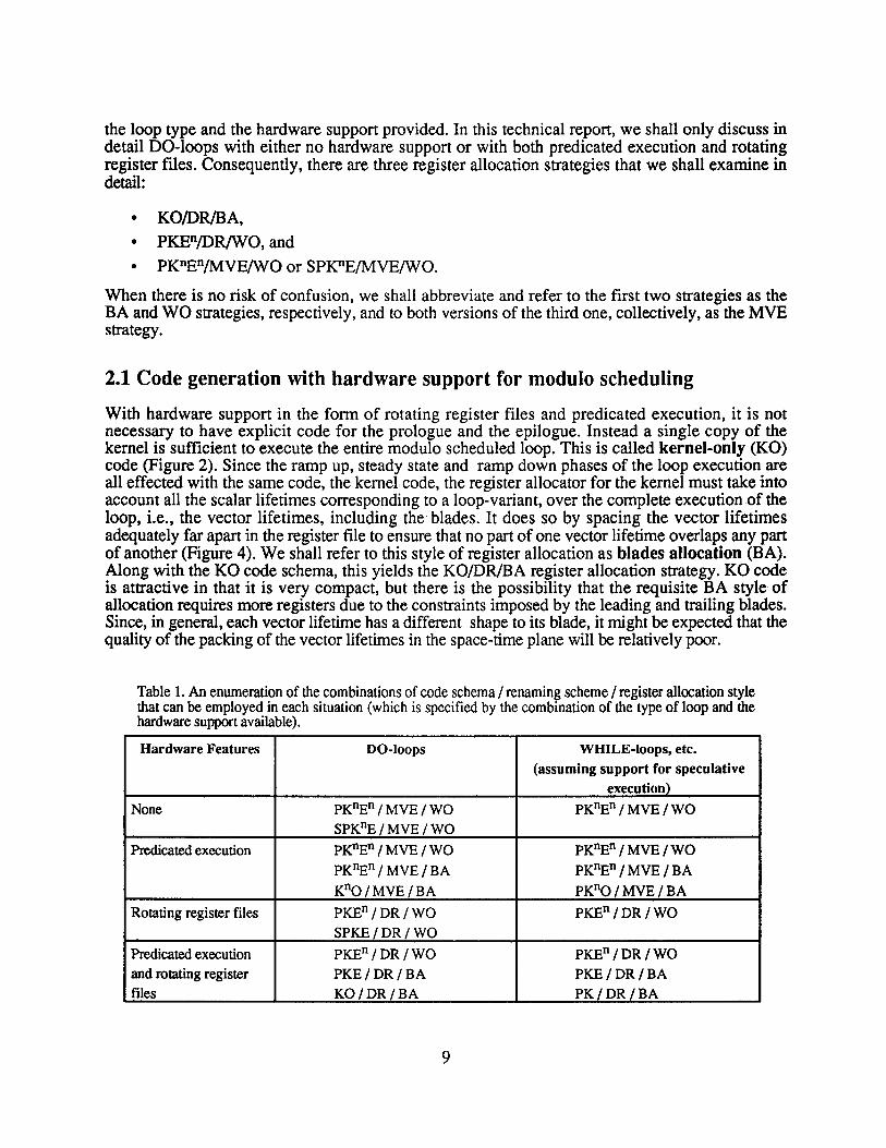
With hardware support in the form of rotating register files and predicated execution, it is notnecessary to have explicit code for the prologue and the epilogue. Instead a single copy of thekernel is sufficient to execute the entire modulo scheduled loop. This is called kernel-only (KO)code (Figure 2). Since the ramp up, steady state and ramp down phases of the loop execution areall effected with the same code, the kernel code, the register allocator for the kernel must take intoaccount all the scalar lifetimes corresponding to a loop-variant, over the complete execution of theloop, i.e., the vector lifetimes, including the blades. It does so by spacing the vector lifetimesadequately far apart in the register file to ensure that no part of one vector lifetime overlaps any partof another (Figure 4). We shall refer to this style of register allocation as blades allocation (BA);Along with the KO code schema, this yields the KO/DR/BA register allocation strategy. KO codeis attractive in that it is very compact, but there is the possibility that the requisite BA style ofallocation requires more registers due to the constraints imposed by the leading and trailing blades.Since, in general, each vector lifetime has a different shape to its blade, it might be expected that thequality of the packing of the vector lifetimes in the space-time plane will be relatively poor.

Table 1. An enumeration of the combinations of code schema / renaming scheme / register allocation stylethat can be employed in each situation (which is specified by the combination of the type of loop and thehardware support available).

Hardware Features DO·loops WHILE-loops, etc.

(assuming support for speculativeexecution)

None PKnEn / MVE / WO PKnEn / MVE / WO

SPKnE / MVE / WO

Predicated execution PKnEn / MVE / WO PKnEn / MVE / WO

PKnEn / MVE / BA PKnEn / MVE / BA

KnO/MVE/BA PKno / MVE / BA

Rotating register files PKEn /DR/WO PKEn/DR/WO

SPKE/DR/ WO

Predicated execution PKEn/DR/WO PKEn/DR/WO

and rotating register PKE/DR/BA PKE/DR/BAfiles KO/DR/BA PK/DR/BA

9

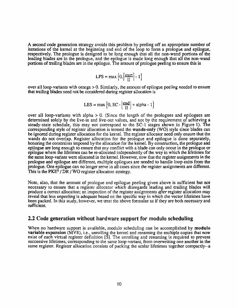
A second code generation strategy avoids this problem by peeling off an appropriate number ofiterations of the kernel at the beginning and end of the loop to form a prologue and epilogue,respectively. The prologue is designed to be long enough that all the non-wand portions of theleading blades are in the prologue, and the epilogue is made long enough that all the non-wandportions of trailing blades are in the epilogue. The amount of prologue peeling to ensure this is

LPS =max {a,r~l- I}

over all loop-variants with omega> a. Similarly, the amount of epilogue peeling needed to ensurethat trailing blades need not be considered during register allocation is

LES = max {a, sc -l~J + alpha - I}

over all loop-variants with alpha > a. (Since the length of the prologues and epilogues aredetermined solely by the live-in and live-out values, and not by the requirement of achieving asteady-state schedule, this may not correspond to the SC-I stages shown in Figure 1). Thecorresponding style of register allocation is termed the wands-only (WO) style since blades canbe ignored during register allocation for the kernel. The register allocator need only ensure that thewands do not overlap. Register allocation for the prologue and epilogue is done separately,honoring the constraints imposed by the allocation for the kernel. By construction, the prologue andepilogue are long enough to ensure that any conflict with a blade can only occur in the prologue orepilogue where the lifetimes can be re-allocated independently of the way in which the lifetimes forthe same loop-variant were allocated in the kernel. However, now that the register assignments in theprologue and epilogue are different, multiple epilogues are needed to handle loop exits from theprologue. One epilogue can no longer serve in all cases since the register assignments are different.This is the PKEn / DR / WO register allocation strategy.

Note, also, that the amount of prologue and epilogue peeling given above is sufficient but notnecessary to ensure that a register allocator which disregards leading and trailing blades willproduce a correct allocation; an inspection of the register assignments after register allocation mayreveal that less unpeeling is adequate based on the specific way in which the vector lifetimes havebeen packed. In this study, however, we treat the above formulae as if they are both necessary andsufficient.

2.2 Code generation without hardware support for modulo scheduling

When no hardware support is available, modulo scheduling can be accomplished by modulovariable expansion (MVE), i.e., unrolling the kernel and renaming the multiple copies that nowexist of each virtual register definition [5]. The unrolling and renaming is required to preventsuccessive lifetimes, corresponding to the same loop-variant, from overwriting one another in thesame register. Register allocation consists of packing the scalar lifetimes together compactly--a

10

more traditional register allocation task'. The minimum degree of unroll, Kmin' is determined by thelongest lifetime among the loop-variants. Because iterations are initiated every II cycles, Kmin canbe calculated as:

K . =MAX ( f(endi-starti)l )min ill'

By unrolling the kernel more than Kmin times, there is the possibility that fewer registers might berequired in the modulo scheduled code, but at the cost of increasing the generated code size and thecompile time of the allocation process. In the absence of hardware support, prologue and epiloguepeeling of SC-l stages are required to ramp up and ramp down the software pipeline. In addition,using the WO style of allocation, live-in and live-out values also impose prologue and epiloguepeeling constraints as explained above. With MVE/WO, the number of stages of prologue andepilogue are given by

PS =max{SC-l, LPS }, andES =max{SC-l, LES}, respectively.

As a result, the blades may be ignored while performing register allocation for the kernel.

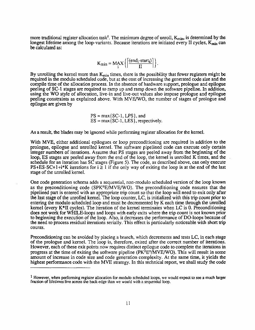
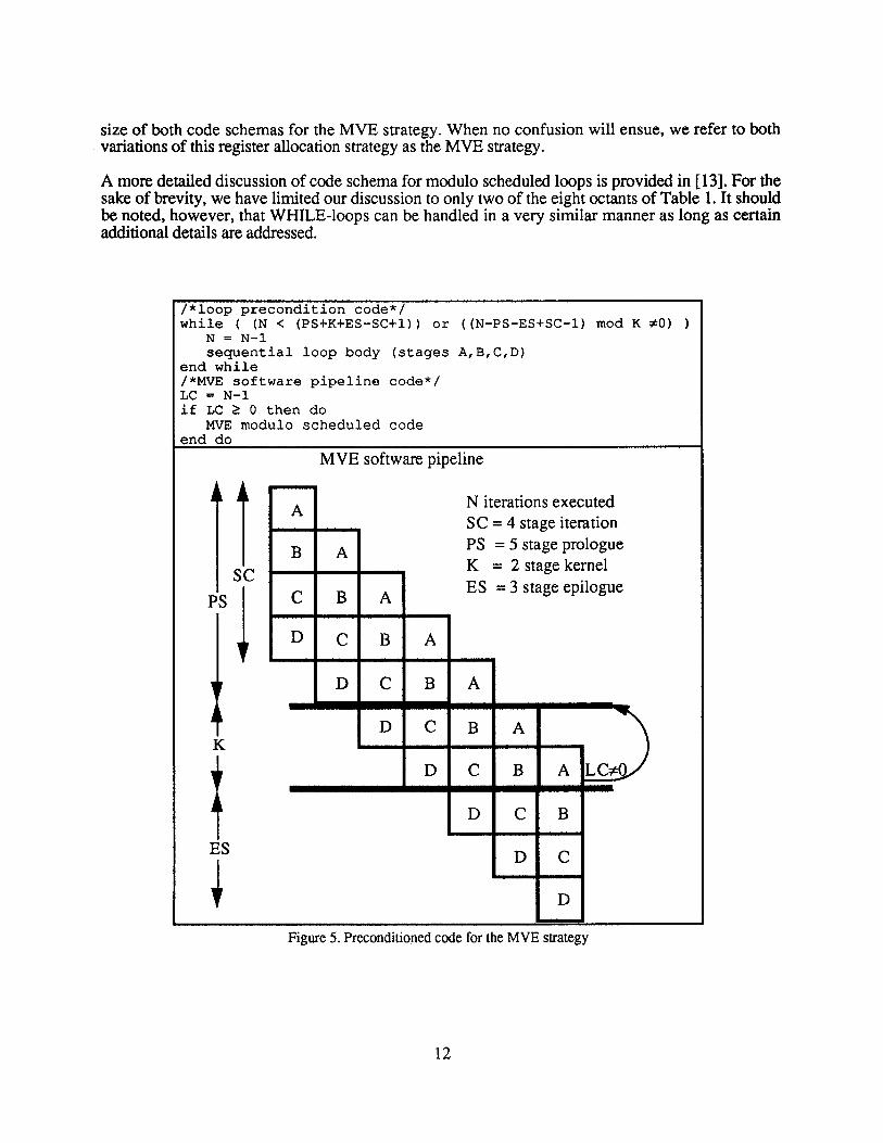
With MVE, either additional epilogues or loop preconditioning are required in addition to theprologue, epilogue and unrolled kernel. The software pipelined code can execute only certaininteger numbers of iterations. Assume that PS stages are peeled away from the beginning of theloop, ES stages are peeled away from the end of the loop, the kernel is unrolled K times, and theschedule for an iteration has SC stages (Figure 5). The code, as described above, can only executePS+ES-SC+1+i*K iterations for i ~ I if the only way of exiting the loop is at the end of the laststage of the unrolled kernel.

One code generation schema adds a sequential, non-modulo scheduled version of the loop knownas the preconditioning code (SPKnE/MVE/WO). The preconditioning code ensures that thepipelined part is entered with an appropriate trip count so that the loop will need to exit only afterthe last stage of the unrolled kerneL The loop counter, LC, is initialized with this trip count prior toentering the modulo scheduled loop and must be decremented by K each time through the unrolledkernel (every K*II cycles). The iteration of the kernel terminates when LC is O. Preconditioningdoes not work for WHILE-loops and loops with early exits where the trip count is not known priorto beginning the execution of the loop. Also, it decreases the performance of DO-loops because ofthe need to process residual iterations serially. This effect is particularly noticeable with short tripcounts.

Preconditioning can be avoided by placing a branch, which decrements and tests LC, in each stageof the prologue and kernel. The loop is, therefore, exited after the correct number of iterations.However, each of these exit points now requires distinct epilogue code to complete the iterations inprogress at the time of exiting the software pipeline (PKnEn/MVE/WO). This will result in someamount of increase in code size and code generation complexity. At the same time, it yields thehighest performance code with the MVE strategy. In this technical report, we shall study the code

1 However, when performing register allocation for modulo scheduled loops, we would expect to see a much largerfraction of lifetimes live across the back-edge than we would with a sequential loop.

11

size of both code schemas for the MVE strategy. When no confusion will ensue, we refer to bothvariations of this register allocation strategy as the MVE strategy.

A more detailed discussion of code schema for modulo scheduled loops is provided in [13]. For thesake of brevity, we have limited our discussion to only two of the eight octants of Table 1. It shouldbe noted, however, that WHILE-loops can be handled in a very similar manner as long as certainadditional details are addressed.

/*loop precondition code*/while ( (N < (PS+K+ES-SC+l» or «N-PS-ES+SC-l) mod K ~O) )

N = N-lsequential loop body (stages A,B,C,D)

end while/*MVE software pipeline code*/LC = N-lif LC ~ 0 then do

MVE modulo scheduled codeend do

,rJ~

K

~ES

~

MVE software pipeline

A N iterations executedSC = 4 stage iteration

B A PS = 5 stage prologueK = 2 stage kernel

C B AES = 3 stage epilogue

D C B A

D C B A

......D C B A

D C B A LC:;cO

D C B

D C

D

Figure 5. Preconditioned code for the MVEstrategy

12

3 Formulation of the register allocation problem

Informally, the register allocation task for modulo scheduled loops with hardware support consistsof packing together the space-time shapes, that correspond to the vector lifetimes, so as to take up aminimum number of registers. An allocation is legal if, out of all the scalar lifetimes that make up allof the vector lifetimes, no two scalar lifetimes that overlap in time are allocated to the same register.This bin packing takes place on the surface of a cylinder with time corresponding to the axis andthe registers corresponding to the circumference. So, the task is to pack the vector lifetimes togetherso that they fit on the surface of a cylinder having the smallest possible circumference. Indescribing the allocation algorithms, we shall need to refer to the linear ordering of registers, and itis important to bear in mind that if, for instance, we have 64 registers, it is equally correct to refer tothe register below 0 as either -lor as 63.

When discussing a vector lifetime, we shall use the lifetime produced by the first iteration of theloop as the point of reference. Thus, we shall say that a vector lifetime has been allocated to physicalregister 7 if the defining operation in the first iteration writes its result to physical register 7.Iterations 2, 3, etc., would write their results to physical registers 6, 5, and so on. Note that, in thisdiscussion, when we refer to registers, we refer to the the absolute addresses of registers which,therefore, are different for each iteration. However, assuming the presence of the kind of registerrenaming that is provided by the rotating register file, the register specifier in the instruction wouldbe invariant. Also, the start and finish times of a vector lifetime refer to those of the scalar lifetimecorresponding to the first iteration.

As another point of terminology, when we say that one vector lifetime is allocated "above" anotherone, we mean that the wand of the first lifetime lies above (and to the right) of the wand for thesecond lifetime in the space-time diagram (see Figure 4b). Note that this does not mean that the firstlifetime is allocated to a higher location than is the second one. If the start time for the first lifetimeis sufficiently later than the start time for the second one, then it can be allocated to a lower locationeven though it is "above" the second lifetime in the space-time diagram. For scalar lifetimes,"above" and "higher location" are synonymous.

3.1 Theregister allocation constraint

Allocation constraints for modulo scheduled loops can be abstracted in order to simplify theformulation of the problem and the implementation of the allocation algorithms. Given fourparameters for each vector lifetime (start, end, omega, alpha), we construct the matrix, DIST, whichhas one row and one column for each vector lifetime. Each off-diagonal element specifies theminimum distance (in registers) allowable between a pair of lifetimes when they are allocated in therotating register file. In Figure 6, vector lifetimes A and B for a schedule with II =3 are shown in aspace-time diagram. (Two possible allocations for B are shown in Figure 6, labelled Be and BU.) Aloop with five iterations is shown. Lifetime A has: (start =8, end = 13, omega = 1, alpha = 1).Lifetime B has: (start =0, end =3, omega =0, alpha =0). The shapes of the lifetimes A and B arecompletely specified by these four parameters. Whereas lifetime B is a wand, i.e., a simple diagonalshape, lifetime A is not, and must carry a value live-in and live-out due to the value of theparameters: omega =1 and alpha =1.

Assume that lifetime A has been allocated to some register in the rotating register file. Lifetime Bcan be allocated adjacent to A either "below" A (Be) or "above" A (B") in Figure 6. When lifetime

13

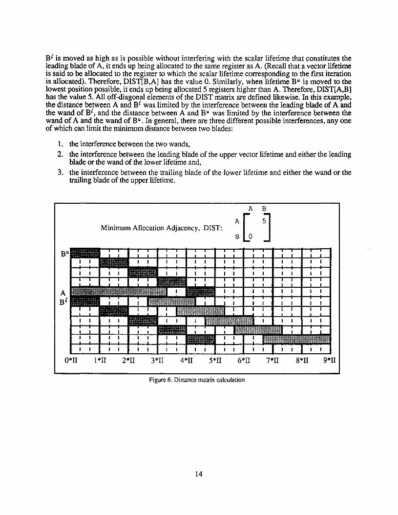
Be is moved as high as is possible without interfering with the scalar lifetime that constitutes theleading blade of A, it ends up being allocated to the same register as A. (Recall that a vector lifetimeis said to be allocated to the register to which the scalar lifetime corresponding to the first iterationis allocated). Therefore, DIST[B,A] has the value O. Similarly, when lifetime Bu is moved to thelowest position possible, it ends up being allocated 5 registers higher than A. Therefore, DIST[A,B]has the value 5. All off-diagonal elements of the DIST matrix are defined likewise. In this example,the distance between A and B{ was limited by the interference between the leading blade of A andthe wand of B{, and the distance between A and Bu was limited by the interference between thewand of A and the wand of Bu. In general, there are three different possible interferences, anyoneof which can limit the minimum distance between two blades:

1. the interference between the two wands,

2. the interference between the leading blade of the upper vector lifetime and either the leadingblade or the wand of the lower lifetime and,

3. the interference between the trailing blade of the lower lifetime and either the wand or thetrailing blade of the upper lifetime.

Minimum Allocation Adjacency, DIST:

A B

:c J

0*11 1*11 2*11 3*11 4*11 5*11 6*11 7*11 8*11 9*11

Figure 6. Distance matrix calculation

14

Accordingly, for vector lifetimes, OIST[A,B] is computed using the following formulae:

d1= rend(A)~tart(B) 1

{dh if omega(B) =0

d2 = max(d1,omega(A)), otherwise

d3 = {d2' if alpha(A) =0max(dz, alpha(A)), otherwise

For WO, OIST[A,B] = dl. For BA, DIST[A,B] = d3.

The OIST matrix for scalar lifetimes, with the MVE strategy, is much simpler. If two scalarlifetimes X and Yare live simultaneously, then DIST[X,Y] =DIST[Y,X] = 1. Otherwise, DIST[X,Y]=DIST[Y,X] =O.

The register allocation problem is to pack the lifetimes, whether vector or scalar, on the surface of acylinder with the minimum circumference while honoring the minimum distance requirements, asspecified by the DIST matrix, between every pair of lifetimes. The appropriate definition of theDIST matrix is used depending on whether the register allocator is working with vector or scalarlifetimes and depending on the register allocation algorithm being used.

3.2 A lower bound on the number of registers needed

A tight lower bound on the number of registers needed for a modulo scheduled loop is useful inassessing the success of the register allocation. A simple, yet surprisingly tight, lower bound isobtained by calculating the total number of scalar lifetimes that are live during each cycle and takingthe maximum of these totals. Clearly, at least this many registers are needed under allcircumstances. This maximum is computed over the entire length of the (possibly unrolled) kernelafter scheduling. In view of the repetitive pattern of lifetimes in an unrolled kernel, the number ofscalar lifetimes that are simultaneously live need only be computed for any II consecutive cycles ofthe kernel.

4 Register Allocation Algorithms

The nature of the overall register allocation process is described in Figure 7. The set of lifetimes tobe allocated are presented to the register allocator in some arbitrary order by the compiler. One canchoose either to retain that order or to put it into a better order which improves the quality of theallocation achieved by a one-pass allocation algorithm. The choice of ordering heuristic iscontrolled by the variable OrderingAlgorithm. Zero, one or multiple heuristics may be selectedsimultaneously. The allocation process consists of repeatedly selecting an as yet unallocatedlifetime, in the order imposed by the ordering heuristics, and allocating it. The choice of registerlocation into which this lifetime is allocated is determined by the allocation algorithm. The variablethat controls this is AllocationAlgorithm. In this study, we only consider one-pass registerallocation algorithms, i.e., algorithms in which each lifetime is allocated exactly once with no back­tracking or iteration.

15

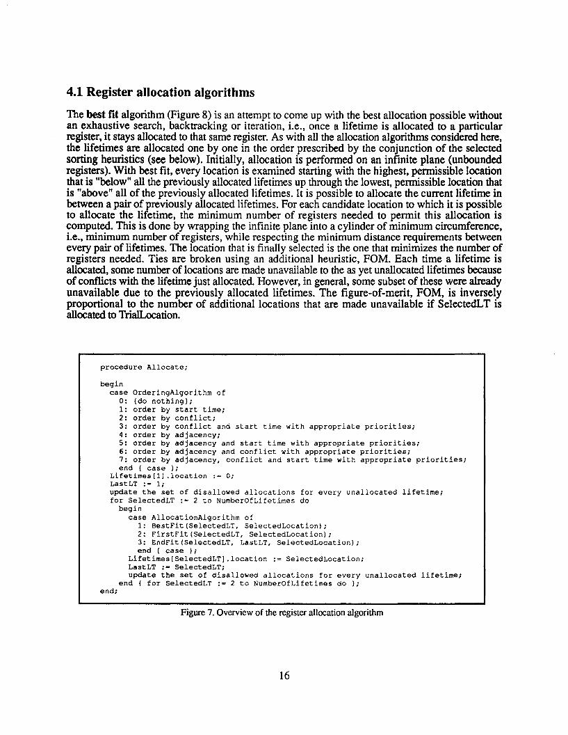
4.1 Register allocation algorithms

The best fit algorithm (Figure 8) is an attempt to come up with the best allocation possible withoutan exhaustive search, backtracking or iteration, i.e., once a lifetime is allocated to a particularregister, it stays allocated to that same register. As with all the allocation algorithms considered here,the lifetimes are allocated one by one in the order prescribed by the conjunction of the selectedsorting heuristics (see below). Initially, allocation is performed on an infinite plane (unboundedregisters). With best fit, every location is examined starting with the highest, permissible locationthat is "below" all the previously allocated lifetimes up through the lowest, permissible location thatis "above" all of the previously allocated lifetimes. It is possible to allocate the current lifetime inbetween a pair of previously allocated lifetimes. For each candidate location to which it is possibleto allocate the lifetime, the minimum number of registers needed to permit this allocation iscomputed. This is done by wrapping the infinite plane into a cylinder of minimum circumference,i.e., minimum number of registers, while respecting the minimum distance requirements betweenevery pair of lifetimes. The location that is finally selected is the one that minimizes the number ofregisters needed. Ties are broken using an additional heuristic, FOM. Each time a lifetime isallocated, some number of locations are made unavailable to the as yet unallocated lifetimes becauseof conflicts with the lifetime just allocated. However, in general, some subset of these were alreadyunavailable due to the previously allocated lifetimes. The figure-of-merit, FOM, is inverselyproportional to the number of additional locations that are made unavailable if SelectedLT isallocated to TrialLocation.

procedure Allocate;

begincase OrderingAlgorithm of

0: {do nothing};1: order by start time;2: order by conflict;3: order by conflict and start time with appropriate priorities;4: order by adjacency;5: order by adjacency and start time with appropriate priorities;6: order by adjacency and conflict with appropriate priorities;7: order by adjacency, conflict and start time with appropriate priorities;end { case };

Lifetimes[1j .location := 0;LastLT := 1;update the set of disallowed allocations for every unallocated lifetime;for SelectedLT := 2 to NumberOfLifetimes do

begincase AllocationAlgorithm of

1: BestFit(SelectedLT, SelectedLocation);2: FlrstFit(SelectedLT, SelectedLocatlon};3: EndFit(SelectedLT, LastLT, SelectedLocation);end ( case );

Lifetimes[SelectedLT].locatlon := SelectedLocation;LastLT := SelectedLT;update the set of disallowed allocations for every unallocated lifetime;

end ( for SelectedLT := 2 to NumberOfLifetimes do );end;

Figure7. Overview of the registerallocation algorithm

16

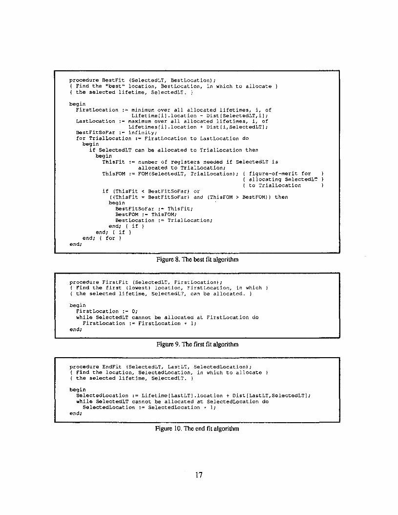
procedure BestFit (SelectedLT, BestLocation);( Find the "best" location, BestLocation, in which to allocate ){ the selected lifetime, SelectedLT. }

figure-of-merit forallocating SelectedLTto TrialLocation

number of registers needed if SelectedLT isallocated to TrialLocation;

:= FOM(SelectedLT, TrialLocation);ThisFOM

beginFirstLocation := minimum over all allocated lifetimes, i, of

Lifetime[i] . location - Dist(SelectedLT,i];LastLocation := maximum over all allocated lifetimes, i, of

Lifetimes[i] . location + Dist(i,SelectedLT];BestFitSoFar := infinity;for TrialLocation := FirstLocation to LastLocation do

beginif SelectedLT can be allocated to TrialLocation then

beginThisFit :=

if (ThisFit < BestFitSoFar) or«ThisFit BestFitSoFar) and (ThisFOM > BestFOM» thenbegin

BestFitSoFar := ThisFit;BestFOM := ThisFOM;BestLocation '= TrialLocation;

end; ( if )end; { if }

end; { for }end;

Figure8. The best fit algorithm

procedure FirstFit (SelectedLT, FirstLocation);{ Find the first (lowest) location, FirstLocation, in which( the selected lifetime, SelectedLT, can be allocated. )

beginFirstLocation := 0;while SelectedLT cannot be allocated at FirstLocation do

FirstLocation := FirstLocation + 1;end;

Figure9. The first fit algorithm

procedure EndFit (SelectedLT, LastLT, SelectedLocation);{ Find the location, SelectedLocation, in which to allocate{ the selected lifetime, SelectedLT. I

beginSelectedLocation := Lifetime [LastLT] .location + Dist[LastLT,SelectedLT];while SelectedLT cannot be allocated at SelectedLocation do

SelectedLocation := SelectedLocation + 1;end;

Figure 10.Theend fit algorithm

17

The tirst tit algorithm (Figure 9) proceeds in a similar fashion except that it always begins itssearch at location 0 and terminates as soon as a location is found to which the lifetime can beallocated

procedure AdjacencyOrder;

beginput all lifetimes in the set NotSetAside;initialize OutputList to empty;remove lifetime 1 from NotSetAside and append it to OutputList;LastLT := 1;for i := 2 to NumberOfLifetimes do

beginMinDistance := infinity;SelectedLT := null;CurrentSet := empty;for j := 1 to NumberOfLifetimes do

if j in NotSetAside thenbegin

if WO or BA strategies thenbegin

ThisDistance := (start[j) - end[LastLT)I + DIST[LastLT,j] * II;if ThisDistance < MinDistance then

beginSelectedLT := j;MinDistance := ThisDistance;

end;end

else { if MVE strategy then Ibegin

conflict[j] := false;ThisDistance := start[j] - end[LastLT];if lifetime[j] conflicts with any lifetime in CurrentSet then

beginconflict[j] := true;ThisDistance := ThisDistance + penalty;

end;if ThisDistance < MinDistance then

beginSelectedLT := j;MinDistance := ThisDistance;

end;end;

end; ( if j in NotSetAside then Iremove SelectedLT from NotSetAside and append it to OutputList;LastLT := SelectedLT;if MVE strategy then

if conflict [SelectedLT) thenCurrentSet := {SelectedLTI

elseCurrentSet := Current Set U {SelectedLTI;

end; { for i := 2 to NumberOfLifetimes do Iend;

Figure11.Theadjacency ordering algorithm

The end tit algorithm (Figure 10) is intended to be used primarily with the adjacency orderingheuristic (see below), with each lifetime being allocated, "above" the last lifetime allocated, to thelowest possible location. Consequently, the search for a location starts with the lowest location suchthat the current lifetime is both above the previously allocated lifetime and does not cause a conflictwith it. This location is specified by the DIST matrix. The search ends at the first legal location thatis encountered, i.e., one which has no conflict with any of the previously allocated lifetimes.

18

4.2 Lifetime ordering heuristics

Three ordering heuristics are considered here: start-time ordering, adjacency ordering and conflictordering. Start-time ordering is motivated primarily by the scalar lifetime case. For a single, non­loop basic block, every lifetime consists of a single interval. In this case, it can be shown thatallocating scalar lifetimes in increasing order of start time, to the lowest available register, yields anoptimal allocation. We shall merely sketch the proof of this theorem. Let L be the lower bound onthe number of registers needed as described in Section 3.2, and let us assume that we are allocatinglifetimes in increasing order of their start times with a budget of L registers to work with. Let T bethe start time of the lifetime that is to be allocated next. Assume that up through the allocation of thepreceding lifetimes, we have not exceeded the lower bound L. So, during the cycle that ends at timeT, there are two possibilities as to the number of busy registers (i.e., registers that hold live values);either there are L busy registers or there are less than L busy registers. If there are less than L busyregisters, any idle register can be selected for the lifetime that we are allocating without exceedingthe lower bound. If there are exactly L busy registers, then, by the definition of the lower bound, atleast one of them must terminate at time T when the lifetime in question starts. The next lifetime canthen be allocated to the newly idled register without exceeding the lower bound. Since, initially, allregisters are idle, this argument can be repeatedly applied to prove that allocation can proceedwithout ever exceeding the lower bound, thereby yielding an optimal allocation.

This procedure is not necessarily optimal for a loop, especially a modulo scheduled one, in whichlifetimes extend across the back-edge of the loop yielding discontiguous lifetimes, i.e., live at thebeginning and end of the loop body but not in between. The complication is that both segments ofthe lifetime must be in the same register. (It can, however, be shown that an upper bound on thenumber of registers needed is L+M, where M is the minimum number of lifetimes that are livesimultaneously [16]1.) In any event, ordering by start time was viewed as a potentially successfulheuristic to use even in this situation and, in fact, was used as the secondary ordering heuristic forvector lifetime allocation in the Cydra 5 compiler.

The primary ordering heuristic in the Cydra 5 compiler was what we shall term adjacencyordering. This greedy heuristic was used in conjunction with the end fit allocation algorithm. Ateach step, that lifetime is selected which minimizes the horizontal distance, in the space-timediagram (Figure 4b), between the lifetime that was allocated last and the one just selected. Bearingin mind that the horizontal dimension is time, we see that this heuristic attempts to minimize theamount of time that any given register is idle.

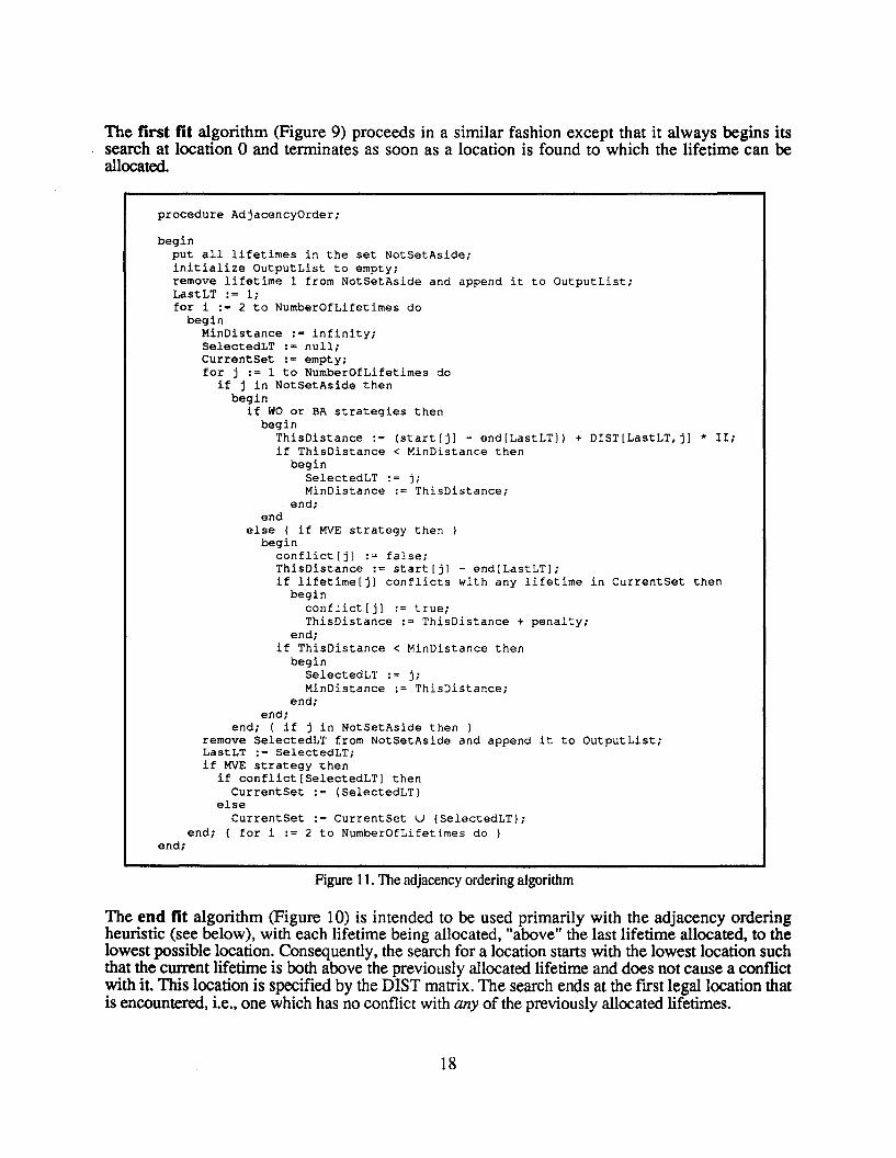
The adjacency ordering algorithm (Figure 11) is quite straightforward for vector lifetimes. Lifetime1 is selected first, Thereafter, the lifetime, B, that is selected at each step is the one for which

(start[B] - end[A]) + DIST[A,B]*II

is minimum, where A is the lifetime that was previously selected. Note that (start[B] - end[A]) is thehorizontal distance in the space-time diagram if A and B were allocated to the same register.DIST[A,B]*II is the additional gap given that B must be allocated to a register that is at least

1 This report also proposes a number of heuristics that are applicable to the MVEstrategy. Having learned of thiswork only during the final preparation of this document, we were unable to evaluate and compare these heuristicswith the ones proposed in this study.

19

DIST[A,B] higher than the one to which A has been allocated. This heuristic is quite similar to theone used with the Travelling Salesman Problem and, in fact, in the WO case, register allocation canbe formulated as a Travelling Salesman Problem.

For scalar lifetimes, too, an attempt is made to minimize the time that a register is idle. In fact, theadjacency ordering algorithm essentially performs a quick-and-dirty allocation. At any point in time,CurrentSet is the set of lifetimes that are tentatively allocated to the same register--the same row inthe space-time diagram. This heuristic keeps appending lifetimes to the right-hand side of the row,always selecting at each step the lifetime that minimizes the gap between the end of the previouslifetime and the selected lifetime. When it is impossible to add an additional lifetime withoutconflicting with one of the lifetimes in that row (taking into account the wrap-around of the lifetimeat K*II), a new row is started.

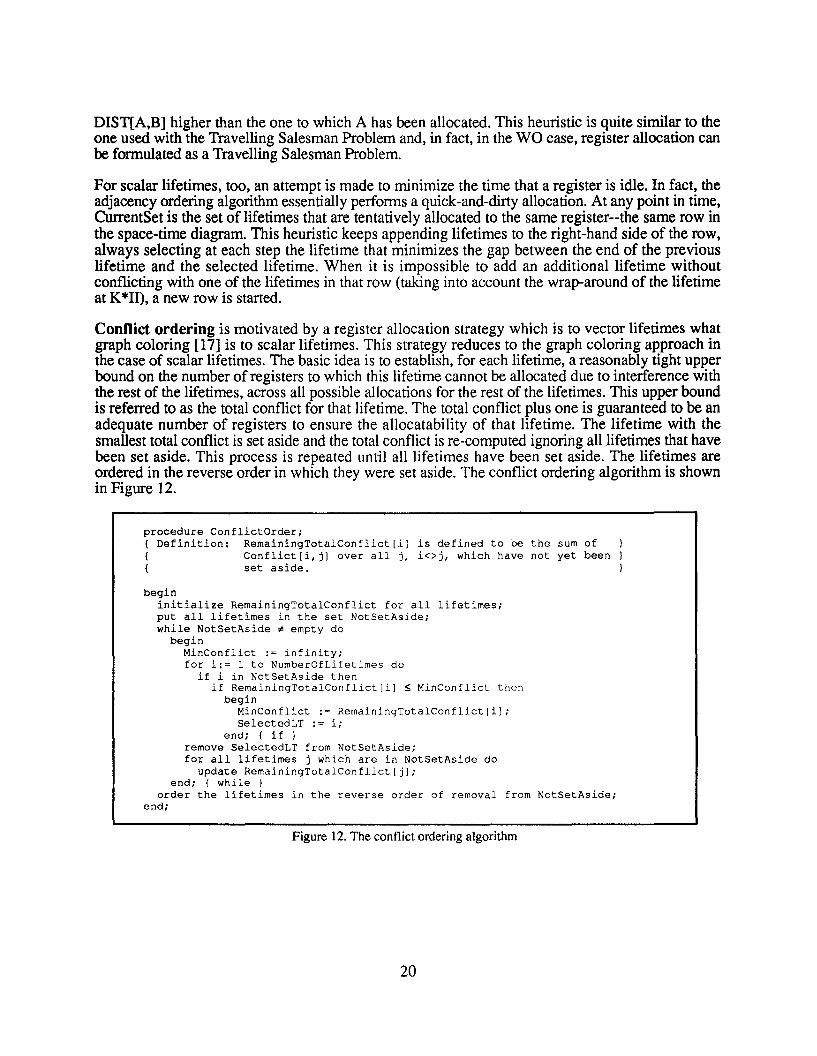
Conflict ordering is motivated by a register allocation strategy which is to vector lifetimes whatgraph coloring [17] is to scalar lifetimes. This strategy reduces to the graph coloring approach inthe case of scalar lifetimes. The basic idea is to establish, for each lifetime, a reasonably tight upperbound on the number of registers to which this lifetime cannot be allocated due to interference withthe rest of the lifetimes, across all possible allocations for the rest of the lifetimes. This upper boundis referred to as the total conflict for that lifetime. The total conflict plus one is guaranteed to be anadequate number of registers to ensure the allocatability of that lifetime. The lifetime with thesmallest total conflict is set aside and the total conflict is re-computed ignoring all lifetimes that havebeen set aside. This process is repeated until all lifetimes have been set aside. The lifetimes areordered in the reverse order in which they were set aside. The conflict ordering algorithm is shownin Figure 12.

procedure ConflictOrder;{Definition: RemainingTotaIConflict[i] is defined to be the sum of{ Conflict[i,j] over all j, i<>j, which have not yet been{ set aside.

begininitialize RemainingTotalConflict for all lifetimes;put all lifetimes in the set NotSetAside;while NotSetAside * empty do

beginMinConflict :; infinity;for i:= 1 to NumberOfLifetimes do

if i in NotSetAside thenif RemainingTotalConflict[i] $ MinConflict then

beginMinConflict := RemainingTotalConflict[i];SelectedLT := i;

end; { if lremove SelectedLT from NotSetAside;for all lifetimes j which are in NotSetAside do

update RemainingTotalConflict[j];end; { while }

order the lifetimes in the reverse order of removal from NotSetAside;end;

Figure 12. The conflict ordering algorithm

20

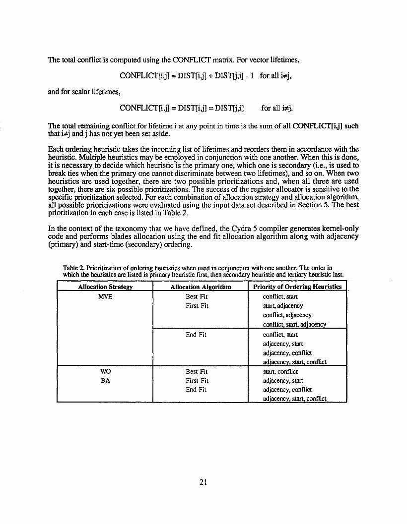
The totalconflict is computed usingthe CONFLICT matrix. For vectorlifetimes,

CONFLICf[i,j] =DIST[ij] +DISTU,i] - 1 for all i;>!:j,

and for scalarlifetimes,

CONFLICf[i,j] =DIST[ij] =DISTU,i]

The totalremainingconflictfor lifetime i at anypoint in time is the sumof all CONFLICf[ij] suchthat i;>!:j andj has not yet been set aside.

Eachorderingheuristic takes the incoming listof lifetimes andreorders themin accordance with theheuristic. Multiple heuristics may be employed in conjunction withone another. When this is done,it is necessary to decide which heuristic is the primaryone, whichone is secondary (i.e., is used tobreak ties when the primaryone cannotdiscriminate between two lifetimes), and so on. When twoheuristics are used together, there are two possible prioritizations and, when all three are usedtogether, thereare six possible prioritizations. The success of the registerallocator is sensitive to thespecific prioritization selected. For eachcombination of allocation strategy and allocation algorithm,all possible prioritizations wereevaluatedusing the input data set describedin Section 5. The bestprioritization in each case is listedin Table2.

In the context of the taxonomy that we have defined, the Cydra 5 compiler generateskernel-onlycode and performs blades allocation using the end fit allocation algorithm along with adjacency(primary) and start-time (secondary) ordering.

Table2. Prioritization of ordering heuristics when usedin conjunction with one another. The orderinwhich the heuristics are listed is primary heuristic first, thensecondary heuristic and tertiary heuristic last.

Allocation StratellV Allocation AIRorithm Prioritv of Orderina Heuristics

MVE Best Fit conflict, startFirst Fit start, adjacency

conflict, adjacencyconflict, start. adiacencv

End Fit conflict, startadjacency, startadjacency, conflictadjacency, start. conflict

WO Best Fit start,conflictBA First Fit adjacency, start

End Fit adjacency, conflictadiacencv. start conflict

21

4.3 Computational Complexity

The worst-case computational complexity for register allocation depends upon the specificcombination of ordering heuristics and allocation algorithm that is employed. From an inspection ofthe algorithms (Figures 7-12) one can see that the worst-case complexity of the three orderingheuristics and the three register allocation algorithms is:

start timeconflictadjacencybest fitfirst fitend fit

CXn2)

CXn2)CXn2)

max(CXn2) , CXn2r»

max(CXn2) , CXnr»max(CXn2) , O(n»

where n is the number of lifetimes (either scalar or vector) to be allocated! and r is the number ofregisters required to do so. Empirically, we found that r was a linear function of n (approximately0.61 *n+14.5) over the range of values of n for which there was statistical significance. So,effectively, best fit, first fit and end fit are CXn3) , O(n2) and CXn2) , respectively. Since the orderingheuristics are CXn2), it is the selected allocation algorithm that dominates the complexity of theregister allocation phase. Note that in the conflict ordering algorithm, updatingRemaining'Totalflonflictlj] for all j that are still in NotSetAside is an CXn) operation.

When multiple ordering heuristics are used together, the lowest priority ordering is performed first,and the highest priority one last. It is necessary, therefore, that each sorting algorithm have theproperty that it maintains the relative ordering of all lifetimes that are equal under the sortingcriterion that is currently being applied. Consequently, a simplistic sort of O(n2) complexity wasused for start-time ordering instead of using heapsort which is O(n log n). The complexityexpressions for the allocation algorithms contain two terms, the greater one of which determines thecomplexity. The CXn2) term is caused by having to update the disallowed locations for each as yetunallocated lifetime each time a lifetime is allocated (Figure 7). The updating process is CXn) incomplexity, and it is invoked n times. The other term is dependent on the allocation algorithmselected. In understanding these, one should note that each of the procedures in Figures 8-10 areinvoked CXn) times and that the loops in Figures 8 and 9 are executed CXr) times on each invocation.Lastly, the function FOM that is called from within the loop in the best fit algorithm is itself CXn) incomplexity.

The worst-case complexity is generally quite pessimistic compared to what is actually experiencedbecause in many cases, the iterations of the loops are guarded by IF-statements that are often notexecuted. So, we also have measured the empirical computational complexity for each combination.This is presented in Section 5. Counters were placed at the entry point as well as in every innermostloop of every relevant procedure. These counters count the total number of times that that point inthe program is visited. In the spirit of worst-case complexity analysis, we used the largest of thecounts as the indicator of empirical computational complexity.

1Note that for the MVE strategy, the number of lifetimes will be Kmin timesgreater thanfor the otherstrategies.

22

5 Experimental Results

Measurements were taken to examine the effectiveness of the allocation algorithms described in theprevious section. To this end, 1358 FORTRAN DO-Ioopsl from the SPEC [18] and PERFECTClub [19] benchmark suites were modulo scheduled on a hypothetical machine similar to the Cydra5 [10]. The relevant details of this hypothetical machine are shown in Table 3. The machine modelpermits the issue of up to seven operations per cycle. All the functional unit pipelines read theirinputs and write their results to a common rotating register file. The 13 cycle load latency reflects anaccess that bypasses the first-level cache. (Our experience has been that locality of reference isoften missing within innermost loops. Until compiler algorithms are devised which reliablyascertain whether or not a sequence of references in a loop has locality, it is preferably to have thedeterministic albeit longer latency that comes from consistently bypassing the first-level cache.) TheCydra 5 compiler was used to generate a modulo schedule for each loop and then output a set oflifetime descriptions for all the loop-variants. The lifetime descriptions were used as input to aprogram that applied all combinations of ordering heuristics and allocation algorithms to each inputset in turn. The register allocation program outputs various data for each input data set and for eachcombination of algorithms and heuristics. The data include the number of registers needed by theloop-variants, a lower bound on the number required, the code size, and the empirical computationalcomplexity.

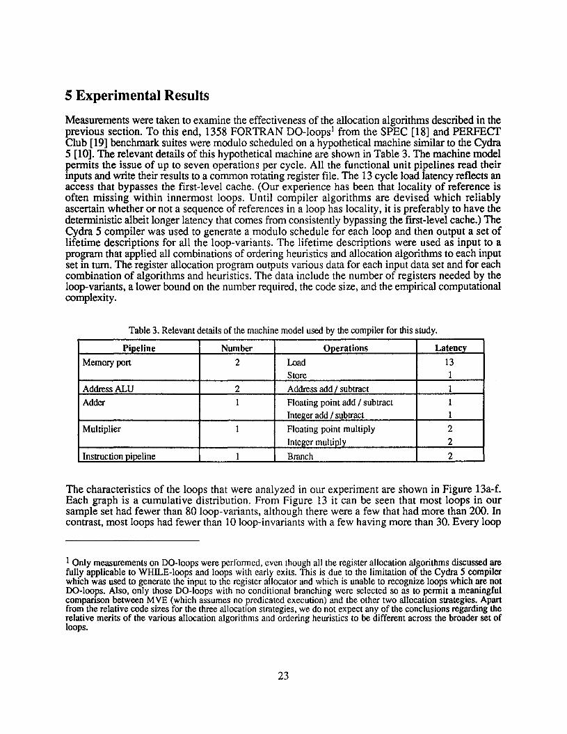
Table 3. Relevant details of the machine model used by the compiler for this study.

Pipeline Number Operations Latencv

Memory port 2 Load 13Store 1

AddressALU 2 Address add / subtract 1

Adder 1 Floating point add / subtract 1Integer add / subtract 1

Multiplier 1 Floating point multiply 2Integer multinlv 2

Instruction nipeline I Branch 2

The characteristics of the loops that were analyzed in our experiment are shown in Figure 13a-f.Each graph is a cumulative distribution. From Figure 13 it can be seen that most loops in oursample set had fewer than 80 loop-variants, although there were a few that had more than 200. Incontrast, most loops had fewer than 10 loop-invariants with a few having more than 30. Every loop

1 Only measurements on DO-loops were performed, even though all the register allocation algorithms discussed arefully applicable to WHILE-loops and loops with early exits. This is due to the limitation of the Cydra 5 compilerwhich was used to generate the input to the register allocator and which is unable to recognize loops which are notDO-loops. Also, only those DO-loops with no conditional branching were selected so as to permit a meaningfulcomparison between MVE (which assumes no predicated execution) and the other two allocation strategies. Apartfrom the relative code sizes for the three allocation strategies, we do not expect any of the conclusions regarding therelative merits of the various allocation algorithms and ordering heuristics to be different across the broader set ofloops.

23

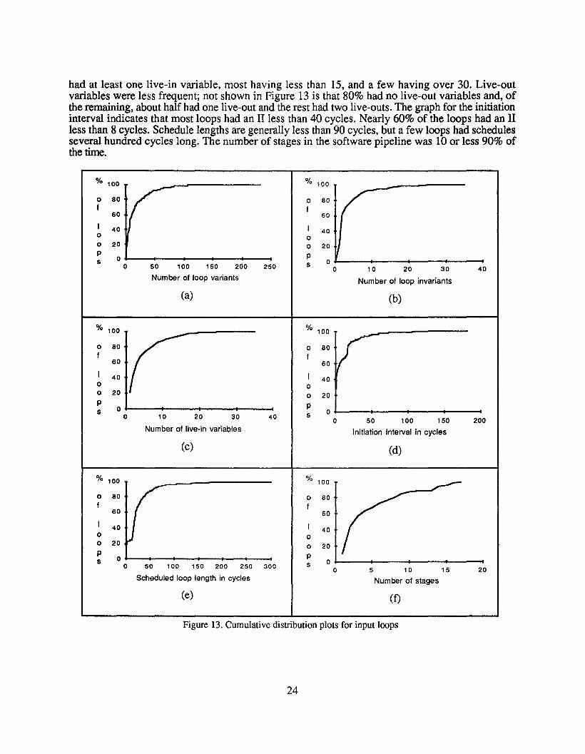
had at least one live-in variable, most having less than 15, and a few having over 30. Live-outvariables were less frequent; not shown in Figure 13 is that 80% had no live-out variables and, ofthe remaining, about half had one live-out and the rest had two live-outs. The graph for the initiationinterval indicates that most loops had an II less than 40 cycles. Nearly 60% of the loops had an IIless than 8 cycles. Schedule lengths are generally less than 90 cycles, but a few loops had schedulesseveral hundred cycles long. The number of stages in the software pipeline was 10 or less 90% ofthe time.

40

200

% 100 % 100

0 80 0 80f f

60 60

I 40 I 400 00 20 0 20P P0s

200 S 00 50 100 150 250 0 10 20 30

Number of loop variants Number of loop invariants

(a) (b)

% 100 % 100

0 80 0 80f f

60 60

I 40 I 400 00 20 0 20P P0s

0 20 30 S 010 40

0 50 100 150Number of live-in variables Initiation Interval in cycles

(C) (d)

% 100 % 100

0 80 0 80f f

60 60

40 400 00 20

0 20P ps 0

0 50 100 150 200 250 300 S5 10 15

Scheduled loop length in cycles Number of stages

(e) (f)

Figure 13. Cumulative distribution plots for input loops

24

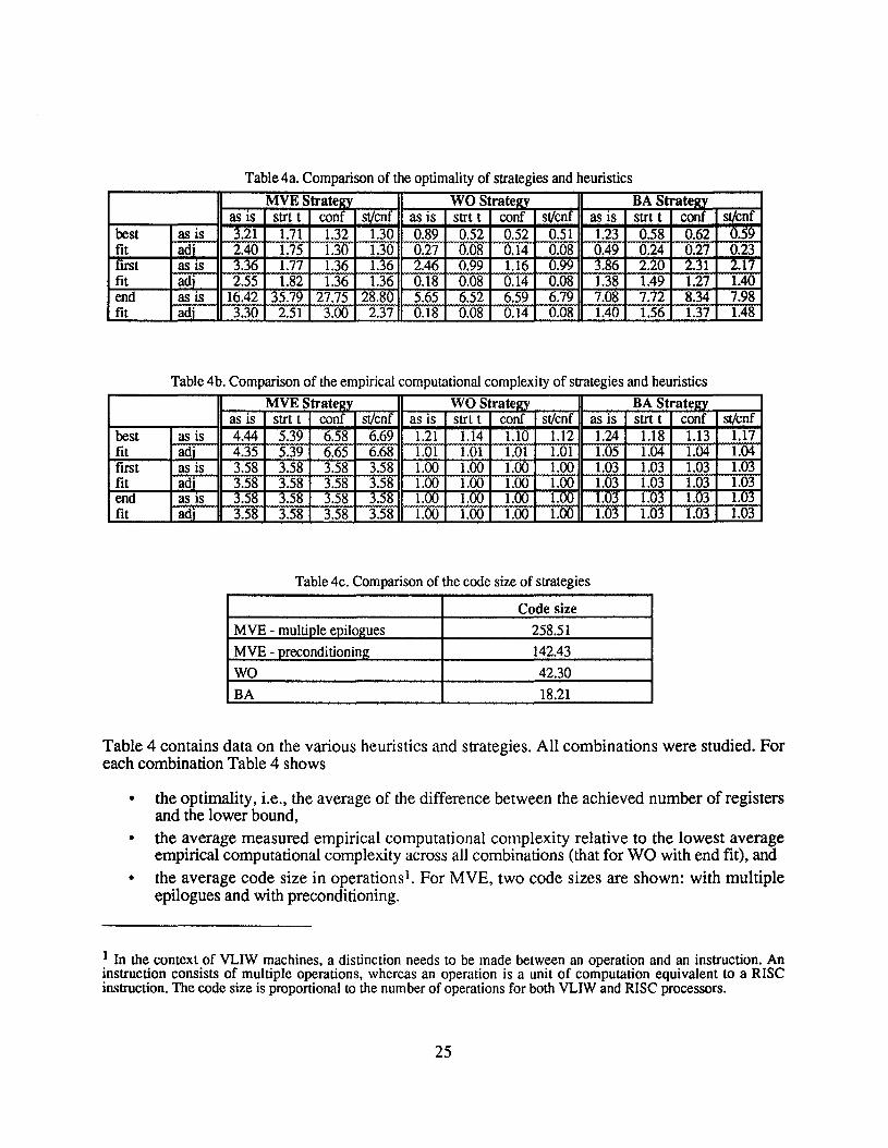
Table 4a. Comparisonof the optimalityof strategiesand heuristics

MVE Stratezv WO Strateav BA Stratezvas is strt t conf stlcnf as is strt t conf stlcnf as is strt t conf stlcnf

best as is 3.21 1.71 1.32 1.30 0.89 0.52 0.52 0.51 1.23 0.58 0.62 0.59fit adi 2.40 1.75 1.30 1.30 0.27 0.08 0.14 0.08 0.49 0.24 0.27 0.23rust as is 3.36 1.77 1.36 1.36 2.46 0.99 1.16 0.99 3.86 2.20 2.31 2.17fit adi 2.55 1.82 1.36 1.36 0.18 0.08 0.14 0.08 1.38 1.49 1.27 1.40end as is 16.42 35.79 27.75 28.80 5.65 6.52 6.59 6.79 7.08 7.72 8.34 7.98fit adi 3.30 2.51 3.00 2.37 0.18 0.08 0.14 0.08 1.40 1.56 1.37 1.48

Table 4b. Comparison of the empiricalcomputational complexity of strategiesand heuristics

MVE Strateav WO Strateev BA Strateavas is strt t conf stlcnf as is strt t conf stlcnf as is strt t conf stlcnf

best as is 4.44 5.39 6.58 6.69 1.21 1.14 1.10 1.12 1.24 1.18 1.13 1.17fit adi 4.35 5.39 6.65 6.68 1.01 1.01 1.01 1.01 1.05 1.04 1.04 1.04first as is 3.58 3.58 3.58 3.58 1.00 1.00 1.00 1.00 1.03 1.03 1.03 1.03fit adi 3.58 3.58 3.58 3.58 1.00 1.00 1.00 1.00 1.03 1.03 1.03 1.03end as IS 3.SH 3.SH 3.58 3.SH 1.00 1.00 1.00 1.00 1.03 1.03 1.03 1.03fit adi 3.58 3.58 3.58 3.58 1.00 1.00 1.00 1.00 1.03 1.03 1.03 1.03

Table 4c. Comparison of the code size of strategies

Code size

MVE - multipleeniloaues 258.51

MVE - preconditioning 142.43

WO 42.30

BA 18.21

Table 4 contains data on the various heuristics and strategies. All combinations were studied. Foreach combination Table 4 shows

• the optimality, i.e., the average of the difference between the achieved number of registersand the lower bound,

• the average measured empirical computational complexity relative to the lowest averageempirical computational complexity across all combinations (that for WO with end fit), and

• the average code size in operations". For MVE, two code sizes are shown: with multipleepilogues and with preconditioning.

1 In the context of VLIW machines, a distinction needs to be made between an operation and an instruction. Aninstruction consists of multiple operations, whereas an operation is a unit of computation equivalent to a RISeinstruction.The code size is proportional to the numberof operations for both VLIW and RISC processors.

25

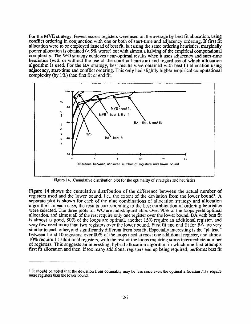
For the MVE strategy, fewest excess registers were used on the average by best fit allocation, usingconflict ordering in conjunction with one or both of start-time and adjacency ordering. If first fitallocation were to be employed instead of best fit, but using the same ordering heuristics, marginallypoorer allocation is obtained « 5% worse) but with almost a halving of the empirical computationalcomplexity. The WO strategy achieves near-optimal results when it uses adjacency and start-timeheuristics (with or without the use of the conflict heuristic) and regardless of which allocationalgorithm is used. For the BA strategy, best results were obtained with best fit allocation usingadjacency, start-time and conflict ordering. This only had slightly higher empirical computationalcomplexity (by 1%) than first fit or end fit.

100

%

80

0

f

60

0

0

P 40

S

20

0 8 12 16 20

Difference between achieved number of registers and lower bound

Figure 14. Cumulative distribution plot for the optimality of strategies and heuristics

Figure 14 shows the cumulative distribution of the difference between the actual number ofregisters used and the lower bound, i.e., the extent of the deviation from the lower bound'. Aseparate plot is shown for each of the nine combinations of allocation strategy and allocationalgorithm. In each case, the results corresponding to the best combination of ordering heuristicswere selected. The three plots for WO are indistinguishable. Over 90% of the loops yield optimalallocation, and almost all of the rest require only one register over the lower bound. BA with best fitis almost as good. 80% of the loops are optimal, another 15% require an additional register, andvery few need more than two registers over the lower bound. First fit and end fit for BA are verysimilar to each other, and significantly different from best fit. Especially interesting is the "plateau"between 1 and 10 registers; over 80% of the loops need at most one additional register, and almost10% require 11 additional registers, with the rest of the loops requiring some intermediate numberof registers. This suggests an interesting, hybrid allocation algorithm in which one first attemptsfirst fit allocation and then, if too many additional registers end up being required, performs best fit

1 It should be noted that the deviation from optimality may be less since even the optimal allocation may requiremore registers than the lower bound.

26

allocation. For MVE, best fit and first fit are almost indistinguishable. 40% of the loops are optimal,and rarely are more than 6 additional registers required. End fit for MVE is significantly worse.

On the average, all three strategies, when they employ the best combination of allocation algorithmand ordering heuristics, are able to achieve extremely good register allocation; On the average, WOis near-optimal, BA requires 0.24 registers more than the lower bound, and MVE requires 1.3registers over the lower bound. The differences lie in their empirical complexity and the resultingcode size.

If we limit our discussion to only the best combinations for each strategy, WO has the lowestempirical complexity, BA is about 4% worse, and MVE is worse by a factor of 6.6. This factordrops to 3.6 if first fit, instead of best fit, is used for MVE. With respect to code size, BA is clearlythe best. WO and MVE require code that is 2.3 and 14.2 times larger, respectively. Ifpreconditioned code is used with MVE, the factor drops to 7.8 (but at the cost of reducedperformance, especially for small trip counts).

For each combination of allocation strategy and allocation algorithm, Table 5 lists the set ofpreferred ordering heuristics. The combination of ordering heuristics selected is the one that yieldsthe best register allocation, on the average. When different combinations of heuristics yield resultsthat are very close in terms of optimality, the least expensive combination, computationally, isselected as the preferred one. In comparing the best fit and first fit algorithms for MVE, one seesthat the two are very close in terms of optimality (a difference of 0.06 registers on the average) butthat first fit has about half the empirical complexity of best fit. Consequently, in Table 5, first fit isunderlined to indicate that it is preferred over best fit. With WO, all three allocation algorithms areequally optimal. So, we prefer end fit since it is the least expensive. With BA, best fit is significantlybetter than the other two for very little added complexity. Accordingly, best fit is the preferredallocation algorithm for BA.

Table5. The preferred allocation algorithm foreachallocation strategy and the preferred orderingheuristics foreach allocation algorithm.

Allocation Strategy Allocation Algorithm Preferred Ordering Heuristics(Preferred)

PKE/MVE Best Fit conflictFirst Fit conflictEnd Fit adjacency, start,conflict

PKE/WO Best Fit adjacency, startFirst Fit adjacency, startEnd Fit adjacency, start

KO/BA Best Fit adjacency, startFirst Fit adjacency, conflictEnd Fit adiacencv, conflict

Comparing the WO and BA strategies (Table 4), it can be seen that the number of registers usedand the measured computational complexity are not very differentbut the average code size forstrategy WO is 2.3 times larger. If one is concerned about instruction cache performance, it may bepreferable to use BA register allocation, and generate KO code. This also allows one to avoid the

27

complexities involved with WO in generating the correct code schema for PKE code [13]. Theperformance degradation of BA relative to WO is limited to the lost opportunity in percolating outerloop computation into the prologue and epilogue. (In both cases, it is assumed that hardwaresupport is available in the form of the rotating register file and predicated execution.)

With the MVE strategy, degrees of unroll greater than Kmin were attempted. Larger degrees ofunroll resulted in higher empirical computational complexity and code size, and provided little to noreduction in the number of registers used. For over 80% of the loops, unrolling by more than Kminsaved at most one register. Very few cases were found where the savings were more than threeregisters. Furthermore, the number of registers needed does not decrease monotonically as thedegree of unroll is increased. Additional unrolling beyond Kmin is not worthwhile.

Figure 15 shows the cumulative distributions for the number of registers used, the code size and theempirical computational complexity for the preferred allocation algorithm and ordering heuristicsfor each strategy. For the machine model used, 98% of the loops required less than 64 registers forloop-variants, and less than 12 registers for loop-invariants. The difference between the strategies ishardly noticeable in Figure 15a, but the MVE strategy performs slightly worse than the other two.Figure 15b and Figure 15c show the cumulative distributions of the code size and empiricalcomputational complexity, respectively. The relative ordering of MVE, WO and BA is the same forthe variance and maximum of the code size distribution as it is for the mean: MVE is larger thanWO which is larger than BA. The same is true for the empirical computational complexity; themean, variance and maximum for MVE are all greater than the corresponding values for BA which,in tum, are marginally greater than those for WOo

6 Discussion

The results of the previous section show that with MVE there is significant code expansion as wellas an increase in compile time. It must be noted, however, that these results correspond only to themodulo scheduled innermost loops. The relative code size and compilation time increases for thecomplete program would be less depending on what fraction of the code consists of innermostloops. Furthermore, the increase in the static code size is relatively unimportant; what matters is theeffect of code size on instruction cache performance. With MVE, when preconditioning is not done,there is a significant code size expansion because there are multiple epilogues. However, if the loopis always executed with the same trip count or with varying trip counts that result in the sameepilogue being executed, then the effective, dynamic code size increase is small. The remainingepilogues do not affect instruction cache performance even though they increase the static code size.If, on the other hand, the loop is executed repeatedly with a variety of trip counts requiring differentepilogues, then this will affect the instruction cache's performance. The extent to which this is aproblem requires further study.

When the loop is preconditioned to avoid the multiple epilogue problem with MVE, the executiontime of the loop varies as a sawtooth (Figure 16) depending on the trip count modulo the degree ofkernel unroll [13]. When the trip count is of the form (PS+ES-SC+l)+i*K (as discussed inSection 2.2), the preconditioning code is not executed, and all loop iterations are executed in asoftware pipelined manner yielding high performance. In the worst case, a number of iterations (oneless than max{K, (PS+ES-SC+l)+K)) have to be executed sequentially, at reduced performance,in the preconditioning code.

28

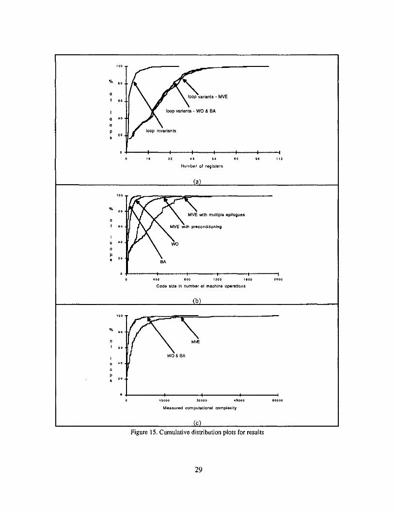
100

% 80

0

1 80

0 ao

0

p20

S

100

%80

0

1 80

0 ao

0

ps 20

Number 01 registers

a

SA

aoo 800 1200 1800 2000

100

%80

0

1 80

0 ao0

p20

S

Code size in number 01 machine operations

b

15000 30000 45000 80000

Measured computational complexity

cFigure 15. Cumulative distribution plots for results

29

50403020

".,,~

_'" - ~--- Prologue-Kernel-Epilogue".

10

.. -o

o

10

30

20

80

40

50

60

70

Trip Count

Figure 16: Execution time as a function of trip count, in the case when II =1, SC =7, Kmin =5, forvarious codeschema: preconditioned, kernel-only andprologue-kernel-epilogue.

The issue of phase-ordering between instruction scheduling and register allocation has been studiedin the context of single basic blocks. There are advocates both for performing register allocationbefore scheduling [20, 21, 7] as well as for performing it after scheduling [22-25]. Each phase­ordering has its advantages and neither one is completely satisfactory. The major problem withperforming register allocation first is that it introduces anti-dependences and output dependencesthat can constrain parallelism and the ability to construct a good schedule. The drawback ofperforming register allocation after scheduling is that, in the event that a viable allocation cannot befound, spill code must be inserted. At this point, the schedule just constructed may no longer beviable. Simultaneous scheduling and register allocation is most attractive, but currently it is onlyunderstood in the context of a linear trace of basic blocks [26]. If a loop is unrolled some numberof times and then treated as a linear trace of basic blocks, simultaneous trace scheduling and registerallocation can be accomplished, but with some loss of performance due to the emptying of pipelinesacross the back-edge [27]. In the case of modulo scheduling, no approach has yet been advancedfor simultaneous register allocation. Since doing register allocation in advance is unacceptablyconstraining on the schedule, it must be performed following modulo scheduling [8].

In this technical report, we have studied the optimality of various allocation algorithms andheuristics. This serves as a useful guide in selecting the best algorithm for each situation with anobjective to minimizing the number of registers needed. A different objective, and one that is equally

30

important, is the issue of how one performs register allocation so as to make do with the number ofregisters that are available. The best algorithm from the first viewpoint is best from the secondviewpoint, too. However, once modulo scheduling has been performed, if the register allocator failsto find a solution requiring no more registers than are available, some additional action must betaken. Various options exist.

One approach is to reschedule the loop with an increased initiation interval. The presumption is thatregister pressure is proportional to the number of concurrently executing iterations. A feasibleallocation may then be found at the expense of reduced performance. However, to benefit from thisstrategy, the modulo scheduling algorithm must incorporate heuristics that take advantage of this byattempting to minimize the number of lifetimes that are simultaneously live at any point. Furtherwork is needed to identify and evaluate such heuristics.

Another option is to select the appropriate lifetimes to spill, add the required spill code, performmodulo scheduling again, and then repeat the register allocation. Rescheduling is necessary becausethe additional loads and stores will, in general, increase the initiation interval. Unfortunately, theincreased initiation interval yields a different schedule in which it is possible that a different set oflifetimes might need to be spilled than those that have already been spilled. The heuristics whichspecify the correct set of lifetimes to spill are not understood at all. A further complication is that wenow require a rotating memory buffer to hold the spilled values for the same reasons that motivatethe use of rotating register files. Alternatively, we need to unroll the kernel in a manner similar toMVE. A detailed discussion of this topic is beyond the scope of this paper.

The third possibility, when register allocation fails, may be to split the loop into two or more loops,each one with fewer operations than the original one. The underlying premise is that loops withfewer operations tend to generate less register pressure. It is not entirely clear that this is so; in factthe smaller loops will generally have a lower II, with the net result that the register pressure couldpotentially even increase. Also unclear is how many loops the splitting should yield and the mannerin which the operations should be divided between the smaller loops. Again, much moreinvestigation is required to understand the merits of this approach.

Although a satisfactory solution to this problem is still a difficult open issue, there is oneobservation that is of help. Our experiments show that the achieved allocation is usually very closeto the easily calculated lower bound. A promising approach might be to keep track of the number ofsimultaneously live values during the modulo scheduling phase and to employ a heuristic whichkeeps this lower bound below the number of available registers, perhaps with a small safety margin.This would almost surely guarantee success in the subsequent register allocation phase.

7 Conclusion

When hardware support is present, in the form of predicated execution and the rotating register file,the kernel-only, blades allocation strategy is to be preferred over the wands-only strategy requiringprologue-kernel-epilogue code. It results in about 55% less code size, and with insignificantincreases in the average number of registers used or in the empirical computational complexity. Thebest combination of heuristics to use with best fit allocation is adjacency and start-time orderingheuristics.

The absence of hardware support for modulo scheduling necessitates prologue and epilogue code,kernel unrolling, modulo variable expansion, and either a sequential preconditioning loop or

31

multiple epilogues. Our experimental data indicate that first fit allocation with conflict ordering isthe best choice. Unrolling the kernel more than the minimum number of times necessary does notsignificantly reduce the number of registers required; instead it increases both the empiricalcomputational complexity and the average code size. Our recommendation would be to employ theminimum degree of unroll.

The measurements of computational complexity and average code size lend some weight toarguments in favor of hardware support for modulo scheduling, in the form of the rotating registerfile and predicated execution. Without it, the increased empirical computational complexity (by afactor of 3 to 6) results in longer compile times. The increased average code size (by a factor of 7 to14) can have a negative effect on the instruction hit rate in cache and, hence, on performance. Thesequential execution of the residual iterations in preconditioned code can further degradeperformance for realistic trip counts.

Acknowledgements

The end fit allocation algorithm and the adjacency ordering heuristic, described in this technicalreport, were conceived of by Ross Towle who, along with Warren Ristow and Jim Dehnert,implemented register allocation for vector lifetimes in the Cydra 5 compiler.

32

References

1. A. E. Charlesworth. An Approach to Scientific Array Processing: The Architectural Design ofthe AP-120B/FPS-I64 Family. IEEE Computer 14,9 (1981), 18-27.

2. B. R. Rau and C. D. Glaeser. Some scheduling techniques and an easily schedulablehorizontal architecture for high performance scientific computing. ProceediDl~s of theFourteenth Annual WorkshQP on MicroprolUammin~ (1981), 183-198.

3. A. Nicolau and R. Potasman. Realistic scheduling: compaction for pipelined architectures.Proceedin~s of the 23th Annual Workshop on Microprogramming and Microarchitecture(Orlando, Florida, 1990),69-79.

4. P. Y. T. Hsu, Hi~hly Concurrent Scalar Processing. Technical Report CSG-49. CoordinatedScience Lab., University of TIlinois, Urbana, Illinois, 1986.

5. M. Lam. Software pipelining: an effective scheduling technique for VLIW machines.Proceedings of the ACM SIGPLAN '88 Conference on Programming Language Design andImplementation (1988), 318-327.

6. R. L. Lee, A. Y. Kwok, and F. A. Briggs. The floating point performance of a superscalarSPARC processor. Proceedings of the Fourth International Conference on ArchitecturalStWPQrt fQrProlUamming Languages and Operating Systems (Santa Clara, California, 1991),28-37.

7. S. Jain. Circular scheduling: A new technique tQ perform software pipelining. Proceedings ofthe ACM SIGPLAN '91 CQnference on Programming Language Design and Implementation(1991),219-228.

8. J. C. Dehnert, P. Y.-T. Hsu, and J. P. Bratt. Overlapped loop support in the Cydra 5.Proceedings of the Third International Conference on Architectural SuPPort for Pro~mmin~Lanfrna~s and Operating Systems (Boston, Mass., 1989), 26-38.

9. P. Tirumalai, M. Lee, and M. S. Schlansker. Parallelization of IQQps with exits Qn pipelinedarchitectures. Proceedings of the SupercQmputing '90 (1990), 200-212.

10. B. R. Rau, et al. The Cydra 5 departmental supercomputer: design philosophies, decisions andtrade-offs. IEEE CQmputer 22, 1 (1989).

11. 1. R. Allen, et al. Conversion of control dependence to data dependence. Proceedings of theTenth Annual ACM Symposium on Principles of Programming Langua~es (1983).

12. K. Ebcioglu and T. Nakatani. A new compilation technique for parallelizing 10Qps withunpredictable branches on a VLIW architecture. Proceedings of the Second WorkshQP onPrQ~ammingLanguages and CQmpilers for Parallel Computing (Urbana-Champaign, 1989),213-229.

13. B. R. Rau, et al., Code GeneratiQn Schema for Modulo Scheduled DO-Loops and WHILE­Loops. Technical Report HPL-92-47. Hewlett-Packard Laboratories, Palo Alto, California,1992.

33

14. B. R. Rau. Data flow and dependence analysis for instruction level parallelism. Proceedinis ofthe Fourth Workshop on Lan&uaieS and Compilers for Parallel Computini (Santa Clara,1991).

15. D. Callahan, S. Carr, and K. Kennedy. Improving Register Allocation for SubscriptedVariables. Proceedings of the ACM SIGPLAN '90 Conference on Programming LanguaieDesign and Implementation (1990), 53-65.

16. L. J. Hendren, et al., Reiister Allocation usini Cyclic Interval Graphs: A New Approach to anOld Problem. Technical Report ACAPS Technical Memo 33. Advanced ComputerArchitecture and Program Structures Group, McGill University, Montreal, Canada, 1992.

17. G. J. Chaitin. Register allocation and spilling via graph coloring. Proceedings of theSIGPLAN82 Symposium on Compiler Construction (1982), 201-207.

18. J. Uniejewski. SPEC Benchmark Suite: Designed for Today's Advanced Systems. SPECNewsletter 1, I (1989).

19. M. Berry, et al. The Perfect Club Benchmarks: Effective Performance Evaluation ofSupercomputers. The International Journal of Supercomputer Applications, 3 (1989),5-40.

20. J. L. Hennessy and T. R. Gross. Postpass code optimization of pipeline constraints. AmTransactions on Pro&Tamming Languages and Systems 5, 3 (1983), 422-448.

21. P. B. Gibbons and S. S. Muchnick. Efficient instruction scheduling for a pipelinedarchitecture. Proceedings of the ACM SIGPLAN Symposium on Compiler Construction(1986), 11-16.

22. J. R. Goodman and W. C. Hsu. Code scheduling and register allocation in large basic blocks.Proceedings of the 1988 International Conference on Supercomputing (1988), 442-452.

23. P. Sweany and S. Beaty. Post-Compaction Register Assignment in a Retargetable Compiler.Proceedings of the 23th Annual Workshop on Microprogramming and Microarchitecture(Orlando, Florida, 1990), 107-116.

24. D. G. Bradlee, S. J. Eggers, and R. R. Henry. Integrating Register Allocation and InstructionScheduling for RISCs. Proceedings of the Fourth International Conference on ArchitecturalSYPPort for Pro&Tamming Languages and Operating Systems (Santa Clara, California, 1991),122-131.

25. P. P. Chang, D. M. Lavery, and W. W. Hwu, The importance of prepass code schedyling forsuperscalar and superpipelined processors. Technical Report CRHC-91-18. Center forReliable and High Performance Computing, University of Illinois, Urbana, IL, 1991.

26. J. R. Ellis. Bulldog: A Compiler for VLIW Architectures. (The MIT Press, Cambridge, Mass.,1985).

27. J. A. Fisher. Trace scheduling: A technique for global microcode compaction. IEEETransactions on Computers 30, 7 (1981),478-490.

34