arX

iv:0

810.

3685

v1 [

astr

o-ph

] 2

1 O

ct 2

008

For ApJSuppl: final draft — lda, November 3, 2018

The Molecular Properties of Galactic H II Regions

L. D. Anderson1, T. M. Bania1, J. M. Jackson1, D. P. Clemens1, M. Heyer2, R. Simon3, R.

Y. Shah4, & J. M. Rathborne5

ABSTRACT

We derive the molecular properties for a sample of 301 Galactic H ii regions

including 123 ultra compact (UC), 105 compact, and 73 diffuse nebulae. We

analyze all sources within the BU-FCRAO Galactic Ring Survey (GRS) of 13CO

emission known to be H ii regions based upon the presence of radio continuum

and cm-wavelength radio recombination line emission. Unlike all previous large

area coverage 13CO surveys, the GRS is fully sampled in angle and yet covers

∼ 75 square degrees of the Inner Galaxy. The angular resolution of the GRS

(46′′) allows us to associate molecular gas with H ii regions without ambiguity

and to investigate the physical properties of this molecular gas. We find clear

CO/H ii morphological associations in position and velocity for ∼ 80% of the

nebular sample. Compact H ii region molecular gas clouds are on average larger

than UC clouds: 2.′2 compared to 1.′7. Compact and UC H ii regions have very

similar molecular properties, with ∼ 5 K line intensities and ∼ 4 km s−1 line

widths. The diffuse H ii region molecular gas has lower line intensities, ∼ 3 K,

and smaller line widths, ∼ 3.5 km s−1. These latter characteristics are similar

to those found for quiescent molecular clouds in the GRS. Our sample nebulae

thus show evidence for an evolutionary sequence wherein small, dense molecular

gas clumps associated with UC H ii regions grow into older compact nebulae and

finally fragment and dissipate into large, diffuse nebulae.

Subject headings: H ii regions — ISM: abundances, clouds, atoms, evolution,

lines, and bands, structure — radio lines: ISM

1Institute for Astrophysical Research, 725 Commonwealth Ave., Boston University, Boston MA 02215,

USA.

2Department of Astronomy, University of Massachusetts, Amherst, MA 01003, USA.

3Physikalisches Institut, Universitat zu Koln, 50937 Cologne, Germany

4MIT Lincoln Laboratory, 244 Wood Street, Lexington, MA 02420

5Harvard-Smithsonian Center for Astrophysics, 60 Garden St., Cambridge, MA 02138, USA

– 2 –

1. INTRODUCTION

In the classical view of H ii region formation OB stars form inside Giant Molecular

Clouds (GMCs). Any newly formed OB star emits extreme ultraviolet (EUV) radiation

(> 13.6 eV) and ionizes the surrounding medium of a molecular cloud, creating an H ii region.

The ionizing photons have more energy than is necessary to ionize the gas, however, and

thus some excess energy heats the ambient gas. Because of the pressure difference between

the cold, natal molecular cloud (∼ 30 K) and the H ii region (∼ 104K), the ionization front

expands into the molecular cloud.

A photodissociation region (PDR) exists beyond the ionization front. The PDR is

a zone where photons of energies lower than 13.6 eV ionize elements with low ionization

potentials and dissociate molecules (see Hollenbach & Tielens 1997, for a review of dense

PDRs). Within the PDR there are three important boundaries. At AV ≃ 1, a dissociation

front exists where H2 replaces H as the dominant species. Further from the emitting star, at

AV ≃ 4, there is a boundary between C+/C/CO where carbon becomes stored predominantly

in the CO molecule. The final boundary of the PDR occurs at the O/O2 transition, AV ≃ 10.

The PDR is therefore a transition region between the H ii region and the molecular cloud; it

is completely ionized at one boundary and completely molecular at the other. Since all H ii

regions should produce PDRs, in this simplified view all H ii regions should have associated

molecular gas when they first form. As the nebulae evolve, however, the OB stars can travel

far enough to leave the environs of their natal molecular clouds.

Complicating this simple scenario is the fact that molecular clouds are clumpy and inho-

mogeneous on all scales (e.g., Falgarone & Phillips 1996; Kramer et al. 1998; Simon et al.

2001). In a clumpy medium, EUV photons can penetrate to different depths, creating non-

spherical ionization fronts. Additionally, H ii regions evolve by moving away from their natal

cloud environments and displacing the local gas. Understanding the complicated interaction

between young stars, H ii regions, and molecular gas is crucial to the study of massive star

formation and the impact massive stars have on their environment.

The molecular component of H ii regions has been studied in detail by many authors.

Most studies, however, have focused mainly on ultra-compact (UC) H ii regions (e.g., Churchwell, Walmsley, & Cesaroni

1990; Kim & Koo 2003). When compact H ii regions were observed in CO, they were of-

ten only observed with single pointings using single-dish telescopes (e.g., Brand et al. 1984;

Whiteoak, Otrupcek, & Rennie 1982; Russeil & Castets 2004). As our results show, CO

gas is frequently offset from the nominal position of an H ii region. A completely sampled

map is required to understand fully the dynamics and properties of molecular gas associ-

ated with H ii regions. Furthermore, a sample with H ii regions at all evolutionary stages is

necessary to understand how this interaction progresses as the H ii region ages.

– 3 –

Here we describe a large scale study of the molecular properties of diffuse, compact, and

ultra-compact Galactic H ii regions using fully sampled CO maps. We trace these molecular

properties using the 13CO J = 1 → 0 emission mapped by the Boston University–Five

College Radio Astronomy Observatory (hereafter BU–FCRAO) Galactic Ring Survey (GRS:

Jackson et al. 2006). CO is an excellent tracer of molecular material because of its high

abundance and the fact that it is rotationally excited at densities common in molecular

clouds (& 500 cm−3).

2. Milky Way Surveys

2.1. Galactic H II Regions

Our Galactic H ii region source sample is compiled from the H ii region radio recombi-

nation line (RRL) catalog of Lockman (1989) (hereafter L89), which consists of nearly 500

RRL observations with a 3′ beam at positions of known continuum emission. These con-

tinuum emission sources were drawn from the 5 GHz continuum survey of Altenhoff et al.

(1979). All positions in Altenhoff et al. (1979) with a peak flux density greater than 1

Jy beam−1 and many sources with peak flux densities down to 0.8 Jy beam−1 were observed,

unless the source was in a very confused region or was a known supernova remnant (SNR).

Since Altenhoff et al. (1979) has coverage from l = 357.◦5 to 60◦ and |b| < 1◦, the L89

catalog is complete down to a flux limit of at least 1 Jy at 5 GHz in this region of the

Galaxy. This sky coverage entirely overlaps and is much larger than the GRS survey zone

(discussed in §2.2), so the L89 catalog is complete at least down to 1 Jy beam−1 over the

extent of the GRS. The sources in L89 are the classical H ii regions first detected in the

1970’s at cm-wavelengths using RRLs. Although they are often misidentified, these are not

the ultra compact, high density H ii regions that are being studied mostly using radio inter-

ferometers. Below, to distinguish these classical H ii regions from UC nebulae, we will call

the L89 nebulae “compact” H ii regions.

Our nebular sample also includes diffuse H ii regions from Lockman, Pisano, & Howard

(1996) (hereafter L96). This catalog consists of RRL measurements at 6 cm (∼ 6′ beam) and

9 cm (∼ 9′ beam) toward 130 faint, extended continuum sources. Most of these sources are

drawn from Altenhoff et al. (1979) and have peak flux densities greater than 0.5 Jy beam−1.

The L89 survey is actually the pilot study of this diffuse sample; it contains 40 diffuse sources.

Recently a large catalog of 1442 Galactic H ii regions was compiled from 24 published

studies of Galactic H ii regions (Paladini et al. 2003). These H ii regions were found using

single-dish, medium resolution (few arcminute beamwidths) observations. For our purposes,

– 4 –

however, this catalog is not useful because nebular positions are given to an accuracy of only

6′.

Finally, our source sample contains UC H ii regions taken from Wood & Churchwell

(1989a), Kurtz et al. (1994), Watson et al. (2003), and Sewilo, et al. (2004). TheWood & Churchwell

(1989a) UC sources were selected by: (1) the presence of a small or unresolved radio

source, (2) a spectrum consistent with free-free emission, and (3) strong FIR emission.

The UC sources from Kurtz et al. (1994), Watson et al. (2003), and Sewilo, et al. (2004)

were selected based on the Wood & Churchwell (1989b) criteria: IRAS flux density ratios

log(F25/F12) ≥ 0.57, log(F60/F12) ≥ 1.30, and F100 ≥ 1000 Jy (≥ 700 Jy for Watson et al.

(2003)), where Fλ is the IRAS flux density at λµm.

2.2. The 13CO Galactic Ring Survey

We use the BU–FCRAO 13CO Galactic Ring Survey data1 (Jackson et al. 2006) to

characterize the molecular properties of all H ii regions in the GRS. The GRS traces the

5 kpc molecular ring discovered by Burton et al. (1975) and Scoville & Solomon (1975).

This annulus of enhanced CO emission dominates the inner Galaxy’s structure and harbors

most of the Galaxy’s star formation regions. The GRS sky coverage spans 18◦ < l < 55◦ and

|b| < 1◦. Additional, incomplete sky coverage is available for 14◦ < l < 18◦ over the same

latitude range. The GRS covers a total of 74 square degrees. The GRS maps the distribution

of emission from the J = 1 → 0 (ν0 = 110.2 GHz) rotational transition of 13CO. The 13CO

isotopologue is ∼ 50 times less abundant than 12CO and hence has a much smaller optical

depth. This decreased optical depth yields smaller line widths and gives a cleaner separation

of individual velocity components along any specific line of sight compared to previous 12CO

surveys.

The GRS, with a spectral resolution of 0.21 km s−1, an angular resolution of 46 ′′, and a

22 ′′ angular sampling, improves upon all previous large scale CO surveys. It is the only fully

sampled (in solid angle) large scale 13CO survey extant. The GRS improves upon the Bell

Labs 13CO survey (Lee et al. 2001) that has a spectral resolution of 0.68 km s−1, an angular

resolution of 103′′ and 180′′ angular sampling. The GRS also has better resolution than

previous 12CO surveys. For example, the University of Massachusetts Stony Brook survey

(Sanders et al. 1986) has a spectral resolution of 1.0 km s−1, an angular resolution of 45′′ and

180′′ angular sampling. The Columbia/CfA 12CO survey (Dame, Hartmann & Thaddeus

2001) has a spectral resolution of 0.18 km s−1, an angular resolution of 450′′ and 225′′ to

1Data available at http://www.bu.edu/galacticring/

– 5 –

450′′ angular sampling. Compared to GRS, all of these surveys are severely undersampled in

angle. The GRS maps have spectra observed at positions separated by ∼ 12the telescope’s

beamwidth (0.48 HPBW, actually). This, together with high spectral resolution allows us

to separate individual 13CO components cleanly. Thus we can for the first time study the

molecular properties of Galactic H ii regions free from angular sampling bias.

3. H II Region Source Sample

Here we study the molecular properties of all known H ii regions in the zone mapped

by the GRS. Our sample of 301 H ii regions contains 123 UC, 105 compact, and 73 diffuse

nebulae. For UC nebulae without RRL measurements in the original papers, we compile

RRL velocities from Afflerbach et al. (1996) and Araya et al. (2002) or, if the UC and

compact sources were co-spatial, from L89. The compact nebulae are from the L89 catalog.

The majority of our diffuse regions are from L96, but a small number are from the pilot

survey of diffuse regions in L89. This final nebular sample results from further vetting of

the §2 sources using data from several recently completed Galactic scale sky surveys that

overlap the GRS zone.

We verify the existence, classification, and position of each H ii region by examining

the radio continuum and infrared emission at its nominal position. For the radio continuum

emission, we primarily use the 21 cm VLA Galactic Plane survey (VGPS: Stil et al. 2006).

In addition to the 21 cm H i line emission data cubes, the VGPS generated 21cm continuum

images over the range 18◦ < l < 67◦, |b| < 1 − 2 with ∼ 1′ resolution. In addition to the

VLA measurements, the VGPS used a Green Bank Telescope 21 cm survey to provide the

zero spacing data. The VGPS is therefore sensitive to both large and small scale emission.

We also use the 20 cm data from the Multi-Array Galactic Plane Imaging Survey (MAGPIS:

Helfand et al. 2006). These data were collected with the VLA operating in B-, C-, and

D-configurations and have a resolution of ∼ 6′′. The 20 cm MAGPIS data cover the range

5◦ < l < 48.◦5, |b| < 0.◦8. We find MAGPIS to be best suited for verifying UC nebulae,

while the VGPS is better suited for verifying compact and diffuse H ii regions. For the

infrared emission, we use the 8µm data from the Galactic Legacy Infrared Mid-Plane Survey

Extraordinaire (GLIMPSE: Benjamin et al. 2003) and 24µm data from the MIPS Inner

Galactic Plane Survey (MIPSGAL: Carey et al. 2008 in preperation). Both infrared surveys

have coverage beyond the extent of the GRS.

For inclusion in our sample, we require a continuum peak at the position of each H ii

region. The UC regions were identified by their IRAS colors and the compact and diffuse

regions were located in radio continuum maps with 2.′6 resolution. Both of these identification

– 6 –

methods have some level of error that can be reduced through correlation with high resolution

radio continuum data. For UC regions, continuum observations are necessary to confirm

that the nebula is an H ii region, and not a dense protostellar clump. The sources from

Wood & Churchwell (1989a) and Kurtz et al. (1994) were confirmed to be UC regions

with VLA continuum observations, but the majority of sources from Watson et al. (2003)

and Sewilo, et al. (2004) have not yet been confirmed with high resolution ratio data. We

exclude 11 UC sources, 2 compact sources and 2 diffuse sources that do not have significant

continuum emission.

We remove all known SNR from our sample by comparing our positions with the catalog

of Green (2006)2 as well as with two recent catalogs of SNRs by Brogan et al. (2006) and

Helfand et al. (2006). Both of these recent catalogs compute the spectral index of SNR

candidates using 20 cm and 90 cm VLA continuum data and rely on the anticorrelation

of SNRs with infrared emission (8µm MSX data in the case of Brogan et al. (2006) and

21µm MSX data for Helfand et al. (2006)). We exclude 13 SNRs from our sample that

were found in these catalogs, as well as one found in Gaensler, Gotthelf, & Vasisht (1999).

There are a comparable number of sources that are spatially coincident with SNRs, but

which have a strong IR component. We believe these are H ii regions in locations that have

produced multiple generations of stars. These sources are retained in our sample. We also

remove an additional six sources that do not have infrared emission since they most likely

are non-thermal.

Finally, we determine if the classification (UC, compact, diffuse) and position of each

source are correct, and remove duplicate sources. We require UC H ii regions to have small

(. 1′) bright knots of continuum emission, compact regions to be larger bright continuum

sources, and diffuse regions to have faint extended continuum emission. There are many

cases where an UC region was mistakenly identified as a compact or diffuse region in the

L89 and L96 catalogs. This misidentification is due to the fact that UCs are unresolved

with the 2.′6 beam of Altenhoff et al. (1979) from which L89 and L96 drew their positions.

We exclude 69 compact and diffuse nebulae whose positions are coincident with UC regions.

Many of the UC H ii regions found in the GRS are in large complexes with individual UC

components separated by angular distances less than the 46′′ GRS beam. We treat these

complexes as single UC regions because they share a common molecular gas clump at the

GRS resolution.

Table 1 lists the 38 H ii regions we cull from our sample because of the criteria just

described. Table 1 gives the source name, the reason for exclusion from our sample, and the

2Available at http://www.mrao.cam.ac.uk/surveys/snrs/)

– 7 –

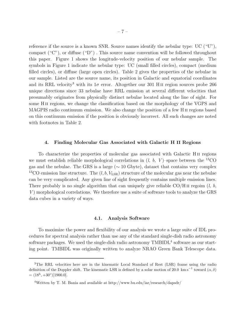
reference if the source is a known SNR. Source names identify the nebular type: UC (“U”),

compact (“C”), or diffuse (“D”) . This source name convention will be followed throughout

this paper. Figure 1 shows the longitude-velocity position of our nebular sample. The

symbols in Figure 1 indicate the nebular type: UC (small filled circles), compact (medium

filled circles), or diffuse (large open circles). Table 2 gives the properties of the nebulae in

our sample. Listed are the source name, its position in Galactic and equatorial coordinates

and its RRL velocity3 with its 1σ error. Altogether our 301 H ii region sources probe 266

unique directions since 33 nebulae have RRL emission at several different velocities that

presumably originates from physically distinct nebulae located along the line of sight. For

some H ii regions, we change the classification based on the morphology of the VGPS and

MAGPIS radio continuum emission. We also change the position of a few H ii regions based

on this continuum emission if the position is obviously incorrect. All such changes are noted

with footnotes in Table 2.

4. Finding Molecular Gas Associated with Galactic H II Regions

To characterize the properties of molecular gas associated with Galactic H ii regions

we must establish reliable morphological correlations in (l, b, V )–space between the 13CO

gas and the nebulae. The GRS is a large (∼ 10 Gbyte), dataset that contains very complex13CO emission line structure. The (l, b, VLSR) structure of the molecular gas near the nebulae

can be very complicated. Any given line of sight frequently contains multiple emission lines.

There probably is no single algorithm that can uniquely give reliable CO/H ii regoim (l, b,

V ) morphological correlations. We therefore use a suite of software tools to analyze the GRS

data cubes in a variety of ways.

4.1. Analysis Software

To maximize the power and flexibility of our analysis we wrote a large suite of IDL pro-

cedures for spectral analysis rather than use any of the standard single-dish radio astronomy

software packages. We used the single-dish radio astronomy TMBIDL4 software as our start-

ing point. TMBIDL was originally written to analyze NRAO Green Bank Telescope data.

3The RRL velocities here are in the kinematic Local Standard of Rest (LSR) frame using the radio

definition of the Doppler shift. The kinematic LSR is defined by a solar motion of 20.0 km s−1 toward (α, δ)

= (18h,+30◦)[1900.0].

4Written by T. M. Bania and available at http://www.bu.edu/iar/research/dapsdr/

– 8 –

(TMBIDL was the inspiration that led to the NRAO GBTIDL5 software.) The TMBIDL

software emulates and improves upon many of the features of the NRAO UniPops analysis

program. It includes Gaussian and polynomial line fitting, data visualization, data manipu-

lation, etc. The TMBIDL code can easily be modified to analyze data from any single dish

radio telescope.

We wrote additional IDL procedures to interface and analyze GRS data within the

TMBIDL environment. TMBIDL was created to analyze single spectra, so we added (l-V ),

(b-V ), and (l-b) mapping tools to better visualize the GRS (l, b, V ) data cubes. The basic

visualization is a normalized contour map of the CO emission. Using these tools, we found

that the morphology of the CO emission at the positions of the H ii regions was often very

complex.

To gain further control over the visualization of the GRS data, we wrote GUI-based

software6 to analyze images extracted from the GRS (l,b,V ) FITS data cubes. This software

provides powerful GUI tools to extract, image, and analyze subcubes for each sample H ii

region. For our analysis we imaged various quantities for an (l,b) zone surrounding each

nebula. The user can, for example, easily modify the velocity channel whose 13CO line

intensity is being imaged over the mapped region. One can also quickly create and display

integrated intensity CO maps, WCO [K km s−1], as well as arbitrarily vary the velocity

range of the integration, ∆V . (This is done with a kernel based algorithm that is fast and

efficient.) Sub-images and regions can be created for any image, saved and then reloaded

at any time. The GUI uses DS97 syntax to define regions. These regions can have all the

basic DS9 shapes. We added a “threshold” region that selects all contiguous pixels above a

user-defined threshold level that surround a given image pixel. Using this thresholding tool

one can identify and analyze arbitrarily complex morphologies.

This GUI-software is fully integrated with TMBIDL. The user can, for example, export

the spectra within any region to TMBIDL for spectral analysis. The ability to scan quickly

through velocity channels, create integrated intensity images, select pixels and fit Gaussians

to spectra — all within a single application — is extremely powerful.

5See http://gbtidl.sourceforge.net/

6Available for download at http://people.bu.edu/andersld/

7Available for download at http://hea-www.harvard.edu/RD/ds9/

– 9 –

4.2. Correlation of Molecular Gas and H II Regions

Our goal is to find a morphological coincidence in (l,b,V ) – space between the CO

gas and the H ii region. After a coincidence is established, we want to characterize the

molecular gas using spectral fits to the 13CO emission. The UC positions are in general

known to an accuracy greater than the 22′′ GRS pixel spacing. For the compact and diffuse

H ii regions, our positions are accurate to a few arcminutes. The RRL LSR velocities are

accurate to ∼ 0.1 km s−1 (from Gaussian fits). Although the (l,b,V ) position of each nebula

is accurately known, establishing a robust set of criteria for identifying a real molecular/H ii

physical association is nontrivial.

The CO emission maps of H ii regions can be quite complex due to GMC structure

and PDR/ionization front interactions. For example, one expects the molecular and ionized

gas velocities to diverge as an H ii region evolves. Once an OB star forms within a GMC

its ionization front (IF) expands rapidly at first, reaching the nebular Stromgren radius in

. 105 yr. The IF pushes the surrounding GMC molecular gas outwards. Dyson & Williams

(1997) show that as the IF expands, it rapidly slows until it is expanding at ∼ 10 km s−1

when it reaches the Stromgren radius. Since H ii regions are generally older than 105 yr

(with the possible exception of some UC H ii regions), the maximum difference between the

RRL and the associated molecular gas should be . 10 km s−1.

Our nebular sample has H ii regions of different ages and thus should show evolutionary

effects. Diffuse H ii regions should be older than the UC nebulae, and thus have had more

time to evolve away from and displace their natal clouds. The molecular gas in diffuse

H ii regions should show a weaker association or may not be present at all. We expect the

majority of UC and compact H ii regions to be associated with a molecular clump (see, e.g.,

Kim & Koo 2003). Because of these complications, our CO/H ii analysis is comprised of a

series of distinct investigations.

4.2.1. Single Position Spectrum Analysis

We first examine the GRS 13CO spectrum at the nominal position of each H ii region.

Most previous studies of the molecular component of H ii regions were made using single

pointings, e.g., Whiteoak, Otrupcek, & Rennie (1982); Russiel & Castets (2004). All report

that the majority of H ii regions have associated CO. Whiteoak, Otrupcek, & Rennie (1982)

found in their survey of 12CO emission from Southern H ii regions that molecular gas within 5

km s−1 of the RRL velocity had large line intensities, and therefore was probably associated

with the H ii region. In their analysis of Southern compact H ii regions using both 12CO and

– 10 –

13CO, Russeil & Castets (2004) argued that 10 km s−1 is a better criterion for determining

a molecular/H ii association.

To make a single pointing CO/H ii comparison we calculate an average 13CO spectrum

at the position of each H ii region by convolving the GRS datacube (which is oversampled

in angle) with the FCRAO telescope beam (HPBW = 46′′). We then search this average

spectrum for a 13CO emission line peak at the H ii region RRL velocity. Specifically, we look

for emission above 0.5K brightness temperature, TMB, and within ±2.5 km s−1 of the H ii

region LSR velocity.

Our brightness temperature limit is chosen to be well above the GRS noise. The GRS

data have a typical RMS sensitivity of σ(TMB) = 0.27K. The beam convolved average

spectrum has a factor of ∼ 2 decrease in noise compared to a single GRS position. Thus

our 0.5K search criterion is a ∼ 3σ limit.

Using the 0.5K and ±2.5 km s−1 criteria, only 52 % of the nebular sample shows a

CO/H ii association. Repeating this procedure with the same intensity requirement, but

with velocity ranges of ±5.0 km s−1 and ±7.5 km s−1, we find that, respectively, 70% and

79% of H ii regions meet these criteria. Certainly increasing the velocity range further still

will yield a greater number of nebulae matching the association criteria, but relaxing the

association definition in this way also increases the chance of a misidentification and the

possibility of blending multiple velocity components.

4.2.2. WCO Integrated Intensity Map Analysis

We use the GRS data to make an (l, b) contour map of the 13CO integrated intensity,

WCO (K km s−1), in order to provide information about the spatial distribution of the molec-

ular gas. The main weakness of the single pointing method of searching for CO/H ii region

associations is that sources with molecular gas offset from the nominal position of the H ii

region are not counted as detections. For each nebula we use TMBIDL to make normalized

WCO contour maps that are l × b = 12′× 12′ (∼ 30× 30 GRS pixels) in size. The map WCO

is calculated by integrating each spectrum over 15 km s−1 centered at the RRL velocity. The

map peak WCO is used to normalize the WCO value for each pixel. The final product is a

normalized contour map for each nebula in the sample.

We then search each map for WCO peaks and note the distance from the 80% peak WCO

contour to the nominal H ii region position. We define any source where this distance lies

within the H ii region positional error bars to be a positive detection and any source where

this distance is just outside of the error bars (roughly twice the positional uncertainty) to be

– 11 –

an ambiguous detection. All sources not meeting these positional criteria are deemed to be

non-detections. We find that 70% of our sample nebulae show positive detections, 14% have

ambiguous detections, and 16% show no correlation between the H ii region position and the13CO emission. Somewhat suprisingly, adding the molecular spatial distribution information

to the CO/H ii association criterion did not add significantly to the detection rate.

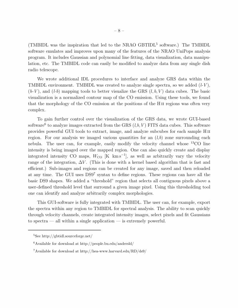
4.2.3. CO (l, b, V ) Data Cube Analysis Procedure

Clearly, the molecular emission in the GRS is complicated and difficult to characterize.

These experiments in establishing a CO/H ii region association demonstrate the need for a

more sophisticated analysis. We use the §4.1 GUI software to search the GRS 13CO data

cubes in (l, b, V ) parameter space. For each nebula we make a series of (l, b) WCO images and

search for CO/H ii region associations. We follow the four step iterative procedure described

below and illustrated in Figure 2.

1. We first find the velocity range of the molecular emission associated with the H ii

region. We examine single velocity channel images (position-position (l, b) maps)

centered at the nominal position of the H ii region at its RRL velocity with overlaid

VGPS 21cm continuum contours. We scan through these single channel images over

±10 km s−1 of the source RRL velocity, searching for the channel where the molecular

emission at the position of the H ii region has the highest intensity. If we are able to

identify a molecular clump near the position of the H ii region, we extract the spectra

from the voxels near this molecular clump. We fit a Gaussian to the (unweighted)

average spectrum of this extracted emission and record the line center and FWHM

of the emission line. Frequently, the molecular emission at the H ii region position is

either absent or has a morphology that is difficult to characterize from single channel

maps. For ∼ 25% of our nebulae we are unable to make a molecular gas association

from these single channel maps.

2. Next we make an integrated intensity map, WCO, by summing the intensities at a given

(l,b) over the range of velocities found in step (1). If the source has an unambiguous

CO/H ii association, we calculate WCO over the velocity range V ± ∆V/2, where V

is the step (1) Gaussian line velocity and ∆V is its FWHM line width. If the source

has an ambiguous step (1) association, we calculate WCO centered at the source RRL

velocity over the range ±10 km s−1.

3. We then use the WCO image created in step (2) to find pixels with molecular emission

associated with the H ii region. We find the brightest emission near the H ii region

– 12 –

in the WCO image and select all contiguous pixels that have values above a threshold

determined independently for each H ii region. The threshold is varied until a small

number of pixels are selected — typically 20 to 30. The exact number is set by the

molecular clump’s intensity profile. Small clumps with a sharply peaked intensity

profile have fewer pixels, whereas larger clumps with a “plateau” of emission have

more pixels. This method seeks to isolate single clumps in order to preserve the line

peak intensity and minimize blending of multiple velocity components.

4. All the GRS spectra within the (l, b) region selected in step (3) are used to calculate

an average 13CO spectrum. We then fit the fewest possible number of Gaussian com-

ponents to the spectrum in order to maximize the intensity of the peak CO emission.

The majority (∼ 80%) of our sources are adequately fit with only one Gaussian com-

ponent. Many nebulae, however, do not have clean Gaussians profiles, but rather show

structure that often suggests a fainter, wider line superposed on a brighter, narrower

line.

Our analysis procedure is summarized in Figure 2 for the H ii region U43.24−0.05.

Panels A and B depict step 1. Panel A shows a single channel GRS map at the velocity

nearest the RRL velocity where the molecular clump has the highest intensity. The cross

marks the nominal H ii region position. For clarity we have not shown the VGPS continuum

emission contours. The black box shows the (l, b) positions of the voxels from which we

extract spectra to produce the average spectrum shown in Panel B. The vertical line in

Panels B and D marks the RRL velocity. Using the velocity range of the emission line shown

as dashed lines in Panel B, we create the integrated intensity image shown in Panel C (step

2). This image has been smoothed with a 3 × 3 Gaussian kernel. The black outline in

Panel C shows contiguous integrated intensity values above a threshold (step 3). This region

and its threshhold is defined by visual inspection of the image. This is the 13CO emission

we deem to be associated with the H ii region. Finally, we extract the spectra from these

(l, b) positions to produce the average spectrum shown in Panel D (step 4). For this source,

our method separates the two emission lines that are blended in the panel B spectrum and

preserves the peak line intensity.

In principle, we could iterate our analysis to locate and fit the molecular emission more

accurately. Using the Panel D Gaussian fit, we could create a new integrated intensity image,

define a new CO/H ii association region, and fit a Gaussian to this new average spectrum.

We did this for 10 test cases and found only only minimal changes that were not significantly

different from a single pass analysis.

This procedure has many advantages. We are able to characterize the spectral prop-

erties of molecular gas distributions that have arbitrary morphologies. We minimize our

– 13 –

assumptions at every stage of the process. By first examining the (l,b) images of each source

at individual velocity channels, we limit false detections that may arise from integrated in-

tensity images containing multiple velocity components blended together. By extracting the

spectra from regions defined in the integrated intensity images, we make no assumptions

based on the visual appearance of the molecular emission at individual velocity channels.

By using a variable threshold to select pixels, we are able to characterize molecular struc-

tures with arbitrary morphology. This threshold definition ensures clean spectral fitting;

the spectra are not contaminated by adjacent pixels that would lower the line intensity and

might increase the width of the fitted Gaussian line. Finally, since we analyze an average of

many spectra, the lines we fit have a much greater signal to noise ratio than a single pointing

spectrum. The Gaussian fit uncertainties in the spectral line parameters we derive are thus

minimized.

After we establish a CO/H ii region association, we characterize the angular size of the

molecular cloud by fitting an ellipse to the WCO spatial distribution. Since the association

defined in Panel C of Figure 2 is a WCO threshold value that is determined independently

for each source, the size of an ellipse fitted to this zone would have little physical meaning.

We therefore define a new threshold selected region that is uniform for the entire nebular

sample. This new region is defined by a threshold set to 80% of the WCO peak inside the

original association zone. The fitting algorithm calculates the semimajor and semiminor

axes using the “mass density” of pixel locations: the clustering of pixel locations along the

l and b directions. The fitted ellipse to this region is thus a uniform estimate of the size of

the molecular gas associated with the H ii region.

The properties we derive for the CO/H ii region associations are summarized in Table

3. For each nebula we list the parameters of the ellipse and Gaussian line fits. All errors are

1σ uncertainties. Given are the ellipse centroid in Galactic coordinates, its size, semi-major,

a, and semi-minor, b, axes, together with the position angle measured from north toward

increasing Galactic longitude. The ellipse size is the geometric mean diameter, 2√ab. If there

are multiple spectral components in the Gaussian fit only the properties of the brightest are

listed. We also use only this brightest component in our subsequent analysis. The fitted line

parameters given are the center velocity, intensity (in main beam brightness temperature

units), and FWHM line width, ∆V . Table 3 also lists some additional nebular properties

derived below in §5: the CO excitation temperature, the 13CO column density, and the

nebular confidence parameter, CP .

– 14 –

5. Discussion

Our analysis here provides a large sample of molecular cloud/H ii region associations

whose physical properties are well characterized. In §4 we show that the molecular emission

is often morphologically complex and offset from the nominal H ii region position and RRL

velocity. We find that the traditional single pointing analysis does not reliably detect the

molecular components of H ii regions. It is very difficult to make a CO/H ii association with

any confidence without an image produced from a (l, b, V ) data cube that spans the entire

H ii region/PDR/molecular cloud interaction region.

To distinguish sources with an unambiguous molecular gas component at the H ii region

position and velocity from those with less robust molecular gas associations, we assign a

confidence parameter, CP , to each source ranging from A to E. Our qualitative criteria

for the confidence parameter are as follows: A: no ambiguity in position or velocity, the

molecular gas coincident with radio continuum or shows clear signs of interaction; B: either

offset somewhat in position or velocity, or in a complex region of molecular gas; C: either

offset in position or velocity or in a complex region, but fainter than a B source and offset

further; D: diffuse emission near the correct position and velocity, but uncharacterizable

due to low intensity or ambiguous morphology; E: nothing at all apparent in position and

velocity.

Figures 3, 4 and 5 give representative examples of our confidence parameter classifi-

cation. These 20′ × 20′ 13CO integrated intensity images span the range of molecular gas

morphologies surrounding our sample of H ii regions. The images are grouped by their confi-

dence parameter classification: Figure 3 shows CP A sources, Figure 4 shows CP B sources

and Figure 5 shows CP C, D, and E sources. Because the GRS is oversampled (22′′ pixels at

46′′ HPBW), we increase the signal to noise by smoothing the images with a 3× 3 Gaussian

filter.

At the top of each image we list the H ii region name, the 13CO line velocity ( km s−1) and

FWHM line width ( km s−1), ∆V , and the source’s confidence parameter. These Gaussian

fitted line parameters are used to calculate the source’s 13CO integrated intensity, WCO(K

km s−1), for the velocity range V ± ∆V/2. At the bottom of each image we give the WCO

calculated from the fitted line: WCO = 1.06 TMB∆v, which is accurate for Gaussian line

shapes. Using the procedure described in Simon et al. (2001), we also give an estimate of

the H2 column density, N(H2)[cm−2].

The grey scale image shows the WCO distribution. Normalized contours are drawn at

83%, 67%, 50%, 33% and 16% of this maximum. (One can get quantitive WCO values using

the scale bar at the right.) For H ii regions where we could not associate molecular gas, the

– 15 –

contour lines are dashed rather than solid and, of course, no line parameters are given.

A bold cross marks the nominal position of the H ii region. Plotted in bold is the

fitted ellipse described in §4.2.3. If there are other H ii regions in the field, they are marked

with thinner crosses. The cross arm lengths correspond to the beam size used to make the

measurement of the H ii region (3′ for L89; 9′ for L96), except for the UC regions where the

cross arm lengths are set to 1′. The GRS beam (HPBW = 46′′) is shown in the lower left

corner of each image. Shown in grey in these images are VGPS 21cm continuum contours.

Tickmarks on these contours point downhill, towards decreasing 21cm emission.

We are able to establish a highly confident (CP A and B) CO/H ii region association

for 62% of the nebulae in our sample. Relaxing the confidence criterion to CP A, B and C

sources gives CO/H ii associations for 84% of our nebular sample. Histograms of the number

distribution of confidence parameter values are shown in Figure 6 for UC (open), compact

(hatched), and diffuse (gray) nebulae. The top left panel is the stacked histogram of the

distribution; the top line represents the entire sample. For example, there are a total of 113

CP A sources: 78 UC, 29 compact, and 6 diffuse H ii regions. Clockwise from here are the

individual histograms for the UC, compact, and diffuse nebulae. (Most subsequent figures

will follow this display format.) As is clear from Figure 6, the UC sample has the greatest

number of high confidence CO/H ii region associations.

Some H ii regions appear to have no molecular gas associated with them. Of our 301

sources, 14 (5%) are classified as E sources; these nebulae show no 13CO emission whatsoever.

Thirty four sources (11%) are classified as D and therefore have only diffuse emission at the

correct position and velocity. Five of our E sources and 15 of our D sources have multiple

RRL velocities along the same line of sight. In these cases, one RRL velocity is probably

from the H ii region of interest while the other is likely from a nearby H ii region. Eleven

of the 12 UC regions with confidence parameter values of D or E have multiple velocity

components.

Two UC H ii regions are worth mentioning individually because of the nature of their

molecular associations. The UC H ii region U33.13+0.09 has a very large velocity offset

between the molecular material and the RRL velocity. L89 find a RRL velocity of 93.8

km s−1 and Araya et al. (2002) find a RRL velocity of 87.4 km s−1. Our 13CO velocity

of 75 km s−1 is in agreement with the CS velocity found by Bronfman, Nyman, & May

(1996). The morphology and linewidth of the molecular emission suggest that the molecular

gas is associated with the H ii region. The UC H ii region U21.42−0.54 also has a compact

molecular clump at the correct (l, b) position. The 13CO velocity of this clump, 54 km s−1,

is 16 km s−1 offset from its RRL velocity of 70 km s−1. This source was not detected

by Bronfman, Nyman, & May (1996). We assign a confidence parameter value of C to

– 16 –

U21.42−0.54 because of the extreme velocity offset.

The lack of CO/H ii region associations in ∼ 20% of our sample is not entirely unex-

pected. This has been reported in the literature before, although previous studies did not

have datasets that were fully sampled in angle as is the GRS. Blitz, Fich, & Stark (1982)

found a lack of associations in 30% of the Sharpless H ii regions studied. Russeil & Castets

(2004) found no association with CO in ∼ 20% of their sample of Southern compact H ii

regions. Churchwell, Walmsley, & Cesaroni (1990) do not detect the dense gas tracer am-

monia in ∼ 30% of a sample of 84 UC H ii regions.

Our large sample of H ii regions contains nebulae spanning a range of evolutionary

stages. The UC regions, being young, are more likely to lie within their natal molecular

clouds where the density of 13CO should be high. As the H ii region evolves, it will dissipate

the gas. We should see evidence for this in the compact and diffuse regions. We therefore

expect UC regions to be associated with small sizes, high excitation temperatures and column

densities, large line widths, and bright line intensities. Diffuse regions should have large sizes

and smaller values for the other quantities compared to the UC regions. Compact regions

should lie in between these two extremes.

The lack of molecular gas in an H ii region can certainly be an evolutionary effect. These

nebulae may represent an older population of H ii regions that have had time to become

displaced from the gas in which they formed due to a variety of mechanisms including, stellar

winds, ionization fronts, high stellar space velocities, etc. One observational consequence

of this scenario might be a bubble morphology in the molecular gas, seen as a ring in

projection. Churchwell et al. (2006) found a large population of bubbles in the GLIMPSE

survey (Benjamin et al. 2003). Observed at mid-infrared wavelengths, GLIMPSE boasts

an angular resolution 10 times that of the GRS and is therefore a better diagnostic tool for

locating bubble features. We indeed see bubbles in 13CO in most H ii regions in the GRS for

sources where Churchwell et al. (2006) also identified bubbles. These regions are usually

classified as D or E sources because the gas has been pushed far away from the center of the

continuum emission. Further investigation of this topic will be the subject of a future paper.

5.1. Properties of Molecular Cloud/H II Region Sources

Here we focus on the 253 nebulae with positive CO/H ii associations, the subset of our

H ii region sample with confidence parameter values of A, B or C. The (l, V ) distribution of

these nebulae is shown in Figure 7 for CP A (large filled circles), B (small filled circles), and

C (small open circles) sources. Fully 90% of UC and compact nebulae have CP A, B, or C

– 17 –

quality CO/H ii associations whereas only 64% of the diffuse nebulae do. Diffuse H ii regions

are probably older on average than either UC or compact nebulae so their significantly lower

associate rate with molecular gas provides the first hint of evolutionary effects in our sample.

Table 4 summarizes the mean properties we derive here for this sample. Listed are

the mean and standard deviation (1σ) for each quantity. This information is given for the

entire sample and also for various subsets of it: UC, compact, and diffuse H ii regions as

well as sources of CP A, B and C. Table 4 lists the number of H ii regions in each category,

the absolute value of the velocity difference between the 13CO molecular clump and the

RRL VLSR, the line intensity (main beam brightness temperature), the FWHM line width,

the size of the associated molecular clump, the CO excitation temperature and the 13CO

column density.

We estimate the average 13CO column density towards our sources using the Rohlfs & Wilson

(1996) analysis:

N(13CO)[cm−2] = 2.42× 1014Tex

∫

τ13 dv

1− exp(−5.29) / Tex(1)

where Tex is the excitation temperature and τ13 is the optical depth of the 13CO line. We

assume the 13CO emission is optically thin and use the Gaussian fit 13CO line parameters

to find the optical depth integral in Eq.1. Both the optical depth and Equation 1, however,

depend on the excitation temperature, Tex.

We use the UMSB 12CO J = 1 → 0 survey (Sanders et al. 1986) to estimate Tex for

each source. We assume 12CO is optically thick and use the radiative transfer equation for

the J = 1 → 0 transition to calculate the excitation temperature from the observed main

beam brightness temperature, T 12MB, of the

12CO line:

Tex = 5.5

/

ln

(

1 +5.5

T 12MB + 0.82

)

. (2)

Eq. 2 holds as long as: (1) the 12CO and 13CO emitting gas is in LTE at the same excitation

temperature; (2) this gas fills the same volume without clumping; and (3) there are no

background continuum sources. (For our nebulae the H ii region continuum is subtracted

when the spectral baselines are removed.)

For each nebula we first compute an average spectrum from the UMSB survey datacube

in exactly the same way as we did for the GRS data. We use the same (l, b) positions

from the identical threshold selected region for this average. We then fit Gaussians to these

– 18 –

average spectra. If we fit multiple Gaussians to the GRS data, we attempt to fit the same

components to the UMSB data. The spectral resolution of the UMSB survey is 1 km s−1, so

this was not always possible as lines resolved in the GRS are blended in the UMSB survey.

Because the pointings of the UMSB survey are further apart than in the GRS (180′′ com-

pared to 22′′), the UMSB survey underestimates the 12CO emission for the small molecular

clumps found in the GRS. For a given velocity, each pixel in the UMSB survey represents

∼ 70 pixels in the GRS. Each threshold selected region contains ∼ 20 GRS pixels on average,

so for the majority of our sources we use only one UMSB pointing to estimate the excitation

temperature appropriate for the 12CO emission. Furthermore, this pointing can be as far

away as ∼ 120′′ from the GRS position.

The distribution of excitation temperatures we derive is shown in Figure 8. All H ii

regions in our sample have very similar excitation temperatures near the standard 10K

value assumed for molecular clouds. We expected the excitation temperature of the UC

regions in particular to be higher than this standard value as the CO gas is nearer to the

exciting star. That we do not see hotter temperatures associated with younger regions is

probably due to the effect of the undersampling of the 12CO emission by the UMSB survey.

The mean 12CO to 13CO ratio for molecular clumps smaller than the beam spacing of the

UMSB survey, 3′, is ∼ 2 while this ratio is ∼ 3 for molecular clumps larger than 3′. Our

excitation temperatures, and hence column densities, are therefore lower limits. Because of

their small size, UCs are affected more by the difference in sampling between the GRS and

the UMSB survey. The UCs also suffer from beam dilution which will lower the inferred

excitation temperature.

Nevertheless, we use these excitation temperatures to compute the 13CO column density

for each source using Eq. 1. These column densities are listed in Table 2. We then estimate

the H2 column density,

N(H2) =

[

12CO13CO

]

×[

H2

12CO

]

×N(13CO), (3)

by assuming constant values for these abundance ratios. Following Simon et al. (2001) we

adopt a 12CO/13CO ratio of 45 and a H2/12CO ratio of 8× 10−5. Our 13CO and H2 column

density results are summarized in Figure 9. As expected, the UC nebulae have on average

the highest column densities and the diffuse nebulae the lowest. Too, the CP A sources have

on average over twice the column density of the CP C nebulae.

We find that the CO gas has on average only a small velocity offset from the H ii region

RRL velocity. Figure 10 shows the difference between the velocity of the CO gas and the

– 19 –

RRL velocity. There is no difference in velocity offset between the various types of H ii

regions. The Gaussian fit to the entire distribution is centered at 0.4 km s−1 with a FWHM

of 8.5 km s−1, whereas the mean of the distribution is 0.2 ± 3.8 km s−1. The fact that the

distribution is centered at zero velocity offset is to be expected for a RRL selected sample

of H ii regions and an optically thin tracer such as 13CO.

This result is in contrast to optically selected samples where a positive velocity offset

was found (e.g., Fich, Dahl, & Treffers 1990). Optical samples choose specific CO/H ii

region line of sight geometries. Face-on or edge-on blister sources such as the Orion nebula

and M17 should dominate these samples. In our sample there is no preferred radial location

for H ii regions within molecular clouds. Because we do not know the CO/H ii geometry

with respect to the line of sight, the absolute value of the CO/RRL velocity difference will

be a direct measure of any systematic velocity offset between the molecular and ionized gas.

Table 4 therefore lists the mean absolute value of the CO/RRL velocity difference; it shows

that there is a ∼ 3 km s−1 average flow velocity between the molecular and ionized gas for

the nebulae in our sample. This value is independent of the type of H ii region, but increases

slightly as the CP value decreases from A to C.

Figure 11 shows the distribution of 13CO line intensities for our sample. Based on

the evolutionary model of H ii regions the natal cloud is gradually dissipated by photo-

dissociation, photo-ionization, and expanding motions. We expect the 13CO density to

decrease as the region progresses from UC to compact and then, finally to diffuse. Assuming13CO is optically thin, or at least marginally so, the higher densities found in UC regions

would lead to higher line intensities, whereas compact sources should show lower line in-

tensities, and diffuse sources the lowest. This hypothesis is only partially borne out as UC

and compact regions share the same distribution, averaging 5.21± 0.23K and 4.96± 0.24K,

respectively. Diffuse regions do show lower line intensities of 3.32± 0.19. The errors quoted

here are the standard errors of the mean, s.e.m. ≡ σ/√N .

Figure 12 shows the distribution of 13CO line widths for our sample. The Gaussian fit

to this distribution is centered at 4.0 km s−1 with a FWHM of 3.2 km s−1. The mean of this

distribution is 4.20±0.09 km s−1. We expected UC H ii regions to have significantly broader

lines than compact H ii regions because the molecular gas is closer to the exciting star and

the outflows should be stronger. Once again, this is not the case: the UC and compact

distributions are very similar, averaging 4.43 ± 0.13 km s−1 (s.e.m) and 4.23 ± 0.14 km s−1

(s.e.m.), respectively. UC and compact regions do have broader lines than the diffuse regions

which average 3.56±0.20 km s−1 (s.e.m.). This suggests that the central star(s) may no longer

be significantly heating molecular gas near diffuse H ii regions.

This distribution of line widths is comparable to that found by Russeil & Castets (2004)

– 20 –

in their single pointing survey of southern H ii regions. They find that the 13CO J = 1 → 0

line has an average line width of 3.7 km s−1 with a standard deviation of 1.9 km s−1. In a

study of UC H ii regions, Kim & Koo (2003) find an average line width of 6.8 km s−1 in

the 13CO J = 1 → 0 transition. Their calculation of line width, however, was based on the

average spectrum over the entire map area, which was as large as 30′ × 40′. For the 8 UC

regions in our sample that Kim & Koo (2003) study, we measure a line width of 5.0 km s−1

whereas they measure 7.2 km s−1. Using the same large areas to compute the line widths

for these sources, we find an average line width of 7.3 km s−1.

The angular size distribution of the H iiCO sources is shown in Figure 13. These sizes

are defined as the geometric mean of the major (2× a) and minor (2× b) axes of the fitted

ellipse, 2√ab. (See §4.2.1 for our ellipse fitting procedure.) There are 6 sources that have

sizes greater than 10′ that are not plotted in Figure 13. These sources are invariably clumps

in a large region of extended molecular emission, which makes our method of determining

the angular size unreliable.

The molecular clumps associated with UC regions do show the smallest sizes, as ex-

pected, averaging 1.′7 ± 0.′1 (s.e.m.). Compact H ii regions are slightly larger, averaging

2.′2± 0.′1 (s.e.m.). The average size of the molecular gas associated with diffuse H ii regions

lies in between that of UC and compact H ii regions, averaging 1.′9 ± 0.′1 (s.e.m.). We have

removed the 6 sources with sizes greater than 10′ from the statistical analysis. The molec-

ular gas around many diffuse regions is fragmented, which leads to the small angular sizes

we measure. Since we only associate a single molecular clump of contiguous pixels with

each nebula, for diffuse H ii regions we probably have not characterized all the associated

molecular gas.

5.2. Comparison with GRS Molecular Clumps

The properties of molecular clumps in the GRS were analyzed down to size scales of

∼ 1′ (Rathborne et al. 2008, in preparation). The contiguous pixel finding algorithm

CLUMPFIND (Williams, de Geus, & Blitz 1994) was used to locate Giant Molecular Clouds

(GMCs) within the GRS. Then, by altering the size threshold in CLUMPFIND, the clumps

within the GMCs were identified and characterized. The distribution of peak intensities and

line widths for these clumps shows a Gaussian core with an exponential tail at high values of

each parameter. The break points where the distributions turn over from being dominated

by the Gaussian core to being dominated by the exponential tail are roughly 4 K and 2

km s−1. By number the vast majority of these GRS molecular clumps have line intensities

below 4 K and line widths below 2 km s−1.

– 21 –

The molecular gas associated with H ii regions has on average a greater line intensity

and larger line width compared to molecular clumps in the GRS. We plot in Figure 14 the

line intensity verses the FWHM line width for the molecular clumps associated with our H ii

regions: UC (filled triangles), Compact (filled circles), and Diffuse (open squares) nebulae.

The solid lines divide the plot into quadrants according to the break points of the GRS

clumps. A similar plot was used by Clemens & Barvainis (1988) to show that the small

clouds in their optically selected molecular cloud sample were cool and quiescent.

The lower left quadrant in Figure 14 should be populated by cold quiescent clouds. These

objects are neither making stars nor being externally heated. The upper left quadrant should

contain a population of clumps that are heated externally. These clouds are warm (or have

high column densities), but do not have the non-thermal motions that would be present

if they posessed a central star. The upper right quadrant should contain molecular gas

associated with embedded massive stars. The lower right quadrant should contain embedded

protostars. These large line width objects are likely active sites of star formation, or near

an active site. Thus the lower, < 4K, part of the plot has a pre-stellar population whereas

the upper part contains clouds that are affected by local massive stars.

The UC and compact nebulae occupy the same region of Figure 14; they have similar

molecular properties. The diffuse regions, however, have lower line intensities and line widths;

they are similar to the general population of molecular clumps. These clumps are no longer

being heated significantly by the ionizing star.

Most of our sources with associated 13CO, 54%, lie in the upper right quadrant of Figure

14 where large line intensities and broad line widths suggest active star formation. The vast

majority of GRS clumps, as well as most of the molecular clouds in Clemens & Barvainis

(1988), reside in the lower left quadrant. The bulk of our remaining nebulae, 42%, lie

in the lower right quadrant. The UC, compact, and diffuse regions all have a significant

population in this quadrant. It is tempting to think that these low line intensities are due

to the decreased optical depth of 13CO but Figure 14 looks very similar to the same plot in

Russeil & Castets (2004) made using the optically thick 12CO J = 2 → 1 transition.

5.3. Are Molecular Cloud/H II Region Associations Real?

Are these CO/H ii region associations really sources that are having a direct physical

interaction between the H ii region and ambient molecular gas? The associations are based

on morphological matches in position and velocity between the 13CO gas, RRL velocity, and

radio continuum emission. But correlation does not imply causality: these matches could in

– 22 –

principle be a coincidental juxtaposition projected on the sky into the same solid angle by

molecular clouds and H ii regions located at entirely different places along the line of sight.

That we require a morphological match in (l, b, V ) – space places a severe constraint on

a false positive association. Mere (l, b) coincidence is not enough; the velocity also needs to

match. The kinematic distance ambiguity in the Inner Galaxy makes it possible for the H ii

region and CO cloud to be at different line of sight positions despite having nearly identical

radial velocities. But these are special places because only they share the same LSR velocity.

Assessing the quantitative probability of a false positive association is beyond the scope of

this paper. To our knowledge no one has yet done the detailed modelling this would require.

One needs to know the Galactic distribution of the clouds which posits a detailed knowledge

of Galactic structure. For a false positive association we require that there not be a cloud

at the H ii region position, but that there be a cloud at the other kinematic distance. One

thus needs to evaluate separately for each H ii region the line of sight distance derivative of

the LSR velocity, dV/dr in order to assess the path lengths at the near and far kinematic

distances that must be populated. This requires a detailed knowledge of Galactic kinematics,

including streaming motions caused by spiral arms. With this information one might be able

to estimate the probability of a false positive association. We probably do not know enough

about either Galactic structure or Galactic kinematics to do this.

The fact, however, that ∼ 20% of the H ii regions do not have associated CO gas

(§5.1) is evidence that suggests chance line of sight superpositions in (l, b, V ) – space are

rare. Furthermore, Figure 14 provides strong support for the physical reality of our CO/H ii

region associations. Our 13CO clouds are not only near to the H ii regions in (l, b, V ) –

space, but their spectra also have the trademarks of star formation: bright lines and large

line widths. This is in marked contrast to the spectral line properties of the vast majority

of GRS clouds (see §5.2). Only 1/3 of the GRS clumps have peak intensities > 4K whereas

55% of our CO/H ii associated clouds do. Only 1/6 of the GRS clouds have line widths

> 2 km s−1; nearly all of our clouds, 96%, exceed this value. We conclude that most of

the CO/H ii region associations must be nebulae with real physical interactions between the

molecular and ionized gas.

6. The GRS H II Region Catalog

Our analysis here produced a catalog of Figure 3 type images and physical properties

for the sample of 301 Galactic H ii regions. We created a website8 to give everyone access

8http://www.bu.edu/iar/hii regions

– 23 –

to this information. In addition to the images of nebular WCO, this website has the average13CO spectrum of each source as well as all the information found in Tables 2 and 3. We

expect this website to be an evolving database compiling additional information about these

nebulae as it becomes available.

7. Future Work

Our sample of CO/H ii region associations will enable many further studies of the prop-

erties of star forming regions at all stages of their evolution. The most important parameter

that is missing here is the distance to each nebula. Knowing the distance would enable us to

derive the intrinsic physical properties of each nebula, establishing their physical sizes and

turning column densities and line intensities into masses and luminosities.

Anderson & Bania (2008)[AB hereafter] use H i absorption studies to derive kinematic

distances toward all the H ii regions with associated molecular gas. All our nebulae are in

the first Galactic quadrant, so their distances are degenerate due to the kinematic distance

ambiguity. Using the fact that H i absorbs thermal continuum from the H ii region, AB use

the VGPS 21cm H i emission line maps to remove this degeneracy (see Kuchar & Bania

1994). This is a proven technique as there is sufficient residual cold H i associated with

almost all GRS molecular clouds to produce significant absorption (Jackson et al. 2002;

Kolpak et al. 2003; Flynn et al. 2004). We shall then use these distances to analyze this

nebular sample and derive the physical properties of the dust and gas (ionized, atomic &

molecular). The completion of the SpitzerGLIMPSE (Benjamin et al. 2003) and MIPSGAL

(Carey et al. 2008 in preperation) surveys, together with the GRS (Jackson et al. 2006),

MAGPIS (Helfand et al. 2006), NVSS (Condon et al. 1998) and the VGPS surveys enable

for the first time a multi-wavelength analysis of the physical properties and evolutionary

state of a large sample of inner Galaxy H ii regions. Due to our large sample size, we will be

able to find examples of H ii regions at all evolutionary stages.

8. Summary

We analyzed the GRS 13CO molecular gas associated with all known H ii regions covered

by the GRS using multiple analysis techniques. Our sample includes 301 regions: 123 UC,

105 compact and 73 diffuse H ii regions. We found that 80% of our H ii regions showed pos-

itive molecular associations, with UCs having the highest association percentage and diffuse

regions the lowest. About 5% of our sample showed no molecular emission whatsoever. We

– 24 –

hypothesize that some of these non-detections represent an older population of H ii regions

where the molecular gas has been displaced from the central star or stars. We found that

the molecular properties of UC and compact H ii regions are quite similar, with line widths

averaging ∼ 4 km s−1 and 13CO column densities of about 3.5 × 1016 cm−2. The molecular

gas associated with diffuse regions has properties more consistent with quiescent clouds. The

molecular gas properties of our sample nebulae are consistent with an evolutionary sequence

wherein small, dense molecular gas clumps associated with UC H ii regions grow into older

compact nebulae and finally fragment and dissipate into large, diffuse nebulae.

This publication makes use of molecular line data from the Boston University-FCRAO

Galactic Ring Survey (GRS). The GRS is a joint project of Boston University and Five Col-

lege Radio Astronomy Observatory, funded by the National Science Foundation under grants

AST-9800334, AST-0098562, & AST-0100793. The National Radio Astronomy Observatory

is a facility of the National Science Foundation operated under cooperative agreement by

Associated Universities, Inc.

REFERENCES

Altenhoff, W.J., Downes, D., Pauls, T., & Schraml, J. 1979, A&AS, 35, 23

Afflerbach, A., Churchwell, E., Accord, J.M., Hofner, P., Kurtz, S., & DePree, C.G. 1996,

ApJS, 106, 423

Anderson, L.D. & Bania, T.M. 2008, ApJ, submitted

Araya, E., Hofner, P., Churchwell, E., & Kurtz, S. 2002, ApJS, 138, 63

Benjamin, R. A., et al. 2003, PASP, 115, 953

Blitz, L., Fich, M., & Stark, A.A. 1982, ApJS, 49, 183

Brand, J., van der Bij, M.D.P., de Vries, C.P., Leene, A., Habing, H.J., Israel, F.P., de

Graauw, T., van de Stadt, H., & Wouterloot, J.G.A. 1984, A&A, 139, 181

Brand, J. 1986, PhD Thesis, Leiden Univ. (Netherlands)

Brogan, C. L., Gelfand, J. D., Gaensler, B. M., Kassim, N. E., & Lazio, T. J, 2006, /apj,

639, 25

Bronfman, L., Nyman, L-A. & May, J. 1996, A&AS, 115, 81

– 25 –

Burton, W. B., Gordon, M.A., Bania, T.M., & Lockman, F.J. 1975, ApJ, 202, 30

Churchwell, E., Walmsley, C.M., & Cesaroni, R. 1990, A&AS, 83, 119

Churchwell, E., et al. 2006, ApJ, 649, 759

Clemens, D. P. 1985, ApJ, 295, 422

Clemens, D. P. & Barvainis, R. 1988, ApJS, 68, 257

Clark, J. S., Egan M. P., Crowther P. A., Mizuno D. R., Larionov V. M., & Arkharov A.

2003, A&A, 412, 185

Condon, J. J., Cotton, W. D., Greisen, E. W., Yin, Q. F., Perley, R. A., Taylor, G. B., &

Broderick, J. J. 1998, AJ, 115, 1693

Dame, T. M., Hartmann, D., & Thaddeus, P. 2001, ApJ, 547, 792

Dyson, J. E., & Williams, D. A. 1997, The Physics of the Interstellar Medium (2nd ed.;

Bristol: Inst. Physics)

Falgarone E. & Phillips, T.G. 1996, ApJ, 472, 191

Fich, L., Dahl, G., & Treffers, R. 1990, AJ, 99, 622

Flynn, E. S., Jackson, J. M., Simon, R., Shah, R. U., Bania, T. M. & Wolfire, M. 2004, ASP

Conference Series, 317, 44

Gaensler, B. M., Gotthelf, E. V., & Vasisht, G. 1999, ApJ,, 526, 37

Green, D.A. 2006, A Catalog of Galactic Supernova Remnants (2006 April version), Mullard

Radio Astronomy Observatory, Cavendish Laboratory (Cambridge, United Kingdom)

Helfand, D.J., Becker, R.H., White, R.L., Fallon, A., and Tuttle, S. 2006, AJ, 131, 2525

Hollenbach, D. J., & Tielens, A. G. G. M. 1997, ARA&A, 35, 179

Jackson, J. M., Bania, T. M., Simon, R., Kolpak, M., Clemens, D. P. & Heyer, M. 2002,

ApJ, 566, 81

Jackson, J. M., Rathborne, J.M., Shah, R.Y., Simon, R., Bania, T.M., Clemens, D.P.,

Chambers, E.T., Johnson, A.M., Dormody, M. & Lavoie, R. 2006, ApJS, 163, 145

Kim, K. & Koo, B. 2003, ApJ, 596, 362

– 26 –

Kolpak, M.A., Jackson, J.M., Bania, T.M., & Clemens, D.P. 2003, ApJ, 582, 756

Kramer, C., Stutzki, J., Rohrig, R., & Corneliussen, U. 1998, A&A, 329, 249

Kuchar, T.A. & Bania, T.M. 1994, ApJ, 436, 117

Kurtz, S., Churchwell, E., Wood, D.O.S. & Myers, P. 1994, ApJS, 91, 659

Kwok, S., Volk, K., & Bidelman W.P. ApJS, 1997, 112, 557

Lee, Y., Stark, A. A., Kim, H., & Moon, D. 2001, ApJS, 136, 137

Lockman, F. J. 1989, ApJS, 71, 469

Lockman, F. J, Pisano, D. J., & Howard, G. J., ApJ, 472, 173

Paladini R., Burigana C., Davies R. D., Maino D., Bersanelli M., Cappellini B., Platania P.,

& Smoot G. 2003, A&A, 397, 213

Rohlfs, K. & Wilson, T.L. 1996, Tools of Radio Astronomy, (3rd ed.; Heidelberg: Springer)

Russeil, D. & Castets, A. 2004, A&A, 417, 107

Sanders, D.B., Clemens, D.P., Scoville, N.Z., & Solomon, P.M. 1986, ApJS, 60, 1

Scoville, N. Z. & Solomon, P. M. 1975, ApJ, 199, L105

Simon, R., Jackson, J.M., Clemens, D.P., & Bania, T.M. 2001, ApJ, 551, 747

Sewilo, M., Churchwell, E., Kurtz, S., Goss, W.M., Hofner, P. 2004, ApJ, 605, 285

Stephenson, C.B. 1992, AJ, 103, 263

Stil, J. M., et al. 2006, AJ, 132, 1158

Watson, C., Araya, E., Sewilo, M., Churchwell, E., Hofner, P., & Kurtz, S. 2003, ApJ, 587,

714

Whiteoak, J. B., Otrupcek, R. E., & Rennie, C. J. 1982, PASAu, 4, 434

Williams, J.P., de Geus, E. J., & Blitz, L. 1994, ApJ, 428, 693

Wood, D.O.S. & Churchwell, E. 1989, ApJ, 69, 831

Wood, D.O.S. & Churchwell, E. 1989, ApJ, 340, 265

This preprint was prepared with the AAS LATEX macros v5.2.

– 27 –

Table 1. Faux and Anomalous Sources

Source Notes Reference

C14.32+0.13 SNR a

D15.45+0.19 SNR a

D15.52−0.14 SNR b

U16.58−0.05 No continuum peak

D17.23+0.39 Probably an evolved star c, d

U17.64+0.15 No continuum peak

C18.64−0.29 SNR a, e

U19.12−0.34 No continuum peak

U19.36−0.02 No continuum peak

C19.88−0.53 No continuum peak

C20.26−0.89 No IR

C20.48+0.17 SNR a, e

D21.56−0.11 SNR a, e

D22.04+0.05 No continuum peak

D2216−0.16 Star c

D22.40−0.37 SNR e

C22.94−0.07 No IR

C23.07−0.37 No IR - Part of SNR?

C23.07−0.25 No IR - Part of SNR?

D23.16+0.02 No continuum peak

U23.24−0.24 No continuum peak

D26.47+0.02 WR or LBV f

U26.51+0.28 No continuum peak

C27.13−0.00 SNR e

C29.09−0.71 SNR e

D29.55+0.11 SNR g

U30.42+0.46 No continuum peak

D30.69−0.63 No IR

U30.82+0.27 No continuum peak

C30.85+0.13 SNR e

C31.05+0.48 SNR e

D31.61+0.33 SNR e

D31.82−0.12 SNR e

U33.24+0.01 No continuum peak

C45.48+0.18 No continuum peak

U49.67−0.45 No continuum peak

C50.23+0.33 No IR

U53.63+0.02 No continuum peak

aBrogan et al. (2006)

bBrogan et al. (2006) (low confidence detection)

cStephenson (1992)

dKwok, Volk, & Bidelman (1997)

eHelfand et al. (2006)

fClark et al. (2003)

– 28 –

gGaensler, Gotthelf, & Vasisht (1999)

– 29 –

Table 2. H ii Region Source Sample

Source l b RA(2000.0) DEC(2000.0) VLSR Reference Comments

(◦) (◦) (h m s) (◦ ′ ′′) ( km s−1)

D15.00+0.05a 15.00 +0.05 18 17 41 −15 52 50 26.5 ± 1.6 L96

D15.00+0.05b · · · · · · · · · · · · 63.5 ± 1.7 L96

D15.64−0.24 15.64 −0.24 18 19 60 −15 27 10 61.8 ± 1.3 L96

C16.31−0.16 16.31 −0.16 18 21 01 −14 49 30 49.5 ± 0.7 L89

C16.43−0.20 16.43 −0.20 18 21 24 −14 44 10 44.5 ± 0.9 L89

D16.61−0.32 16.61 −0.32 18 22 11 −14 38 10 44.9 ± 0.6 L89 a

D16.89+0.13 16.89 +0.13 18 21 05 −14 10 30 42.3 ± 1.6 L96

D17.25−0.20a 17.25 −0.20 18 22 59 −14 00 50 49.9 ± 1.4 L96

D17.25−0.20b · · · · · · · · · · · · 96.5 ± 1.9 L96

U18.15−0.28 18.15 −0.28 18 25 01 −13 15 20 53.9 ± 0.4 L89

aChanged nebular classification from compact

Note. — Table 2 is published in its entirety in the electronic edition of the Astrophysical Journal Supplement

Series. A portion is shown here for guidance regarding its form and content.

–30

–

Table 3. Properties of Molecular Cloud/H iiRegion Sources

Fitted Ellipse Parameters Fitted Gaussian Parameters

Source l b Size Maj. × Min. PA V TMB ∆V Tex N(13CO) CP

(◦) (◦) (′) (′ × ′) (◦) ( km s−1) (K) ( km s−1) K (×1016 cm−2)

D15.00+0.05a 14.93 +0.02 2.1 1.6× 0.7 +88.6 25.85 ± 0.02 6.03 ± 0.02 3.77 ± 0.05 12.7 3.2 B

D15.00+0.05b · · · · · · · · · · · · · · · · · · · · · · · · · · · · · · E

D15.64−0.24 15.66 −0.21 2.0 2.1× 0.5 +70.6 56.96 ± 0.06 1.88 ± 0.06 1.86 ± 0.09 8.6 0.4 B

C16.31−0.16 16.36 −0.21 1.7 0.9× 0.8 +45.0 47.56 ± 0.11 4.17 ± 0.11 4.68 ± 0.12 11.0 2.6 B

C16.43−0.20 16.36 −0.21 1.7 0.9× 0.8 +14.9 48.83 ± 0.02 9.47 ± 0.02 2.74 ± 0.04 13.9 3.9 B

D16.61−0.32 16.56 −0.34 4.8 2.9× 2.0 +26.3 43.23 ± 0.01 5.39 ± 0.01 4.44 ± 0.04 11.1 3.2 C

D16.89+0.13 · · · · · · · · · · · · · · · · · · · · · · · · · · · · · · D

D17.25−0.20a 17.23 −0.24 3.9 2.7× 1.4 −63.4 44.57 ± 0.03 5.62 ± 0.03 4.05 ± 0.07 15.7 3.6 B

D17.25−0.20b · · · · · · · · · · · · · · · · · · · · · · · · · · · · · · D

U18.15−0.28 18.15 −0.31 2.2 1.7× 0.7 +77.9 52.53 ± 0.04 7.32 ± 0.04 4.75 ± 0.06 24.6 7.6 A

Note. — Table 3 is published in its entirety in the electronic edition of the Astrophysical Journal Supplement Series. A portion is shown here for guidance

regarding its form and content.

– 31 –

Table 4. Mean Properties of Nebulae with Associated 13CO

N |V | Offset TMB ∆V Size Tex N(13CO)

( km s−1) (K) ( km s−1) (′) (K) (×1016 cm−2)

All 253 2.98 ± 2.41 4.77 ± 2.32 4.19 ± 1.42 1.9 ± 1.3 12.1 ± 4.8 3.1 ± 2.6

UC 111 3.03 ± 2.61 5.21 ± 2.40 4.43 ± 1.38 1.7 ± 1.1 12.2 ± 5.0 3.5 ± 2.8

Compact 95 3.01 ± 2.37 4.96 ± 2.36 4.23 ± 1.40 2.2 ± 1.6 13.3 ± 4.7 3.3 ± 2.6

Diffuse 47 2.81 ± 2.01 3.32 ± 1.29 3.56 ± 1.37 1.9 ± 1.0 9.3 ± 3.0 1.6 ± 1.0

A 112 2.65 ± 2.06 5.63 ± 2.51 4.52 ± 1.26 1.7 ± 0.8 12.8 ± 5.1 4.0 ± 3.0

B 75 3.00 ± 2.37 4.62 ± 2.06 4.05 ± 1.31 2.1 ± 1.5 12.1 ± 4.4 2.8 ± 2.0

C 66 3.53 ± 2.90 3.46 ± 1.51 3.80 ± 1.66 2.2 ± 1.7 11.0 ± 4.4 1.9 ± 1.9

– 32 –

0 20 40 60 80 100 120Vlsr (km/s)

20

30

40

50

Gal

actic

Lon

gitu

de (

deg)

Fig. 1.— Longitude-LSR velocity diagram for H ii regions located inside the GRS survey

zone. The nebulae are shown projected onto the Galactic plane. The symbols represent UC

nebulae (small filled circles), compact nebulae (medium filled circles), and diffuse nebulae

(large open circles).

– 33 –

0.00

0.67

1.33

2.00

2.67

3.33

4.00

T* A

(K)

43.35 43.30 43.25 43.20 43.15 43.10L (deg)

-0.20

-0.15

-0.10

-0.05

0.00

0.05

0.10

B (

deg)

43.35 43.30 43.25 43.20 43.15 43.10L (deg)

-0.20

-0.15

-0.10

-0.05

0.00

0.05

0.10

B (

deg)

A

0 20 40 60 80Velocity (km/s)

-0.5

0.0

0.5

1.0

1.5

2.0

2.5

T* A

(K)

D

0 20 40 60 80Velocity (km/s)

-0.20.0

0.2

0.4

0.6

0.8

1.01.2

T* A

(K)

B

0.00

10.00

20.00

30.00

40.00

50.00

60.00

Inte

grat

ed In

tens

ity (

K K

m/s

)

43.35 43.30 43.25 43.20 43.15 43.10L (deg)

-0.20

-0.15

-0.10

-0.05

0.00

0.05

0.10

B (

deg)

43.35 43.30 43.25 43.20 43.15 43.10L (deg)

-0.20

-0.15

-0.10

-0.05

0.00

0.05

0.10

B (

deg)

C

Fig. 2.— The CO/H ii association procedure for the U43.24−0.05 H ii region (see text).

Panel A: Using single velocity channels near the RRL velocity and nominal H ii region

position we first locate the associated molecular emission. The black cross shows the H ii

region position. The black rectangle defines the extent of the 13CO emission that is deemed

to be associated with the H ii region. Panel B: The average 13CO spectrum of the GRS data

cube voxels that lie within the panel A black rectange is shown. The solid vertical line flags

the H ii region RRL velocity and the dashed lines show the velocity range of the associated

emission. Panel C: The integrated intensity image made from the data cube using the line

center velocity and FWHM line width found by the Panel B Gaussian fit is shown. This

image is then used to define the final extent of 13CO emission that is deemed to be associated

with the H ii region. The black outline shows this region which is defined by a threshold

algorithm (see text). Panel D: The average 13CO spectrum of the data cube voxels that

lie within the panel C threshold defined region is shown. The vertical line flags the RRL

velocity. The Gaussian fit to the emission line is used to derive the physical properties of

the 13CO gas associated with this H ii region. The spectrum from panel B is shown in gray

for comparison.

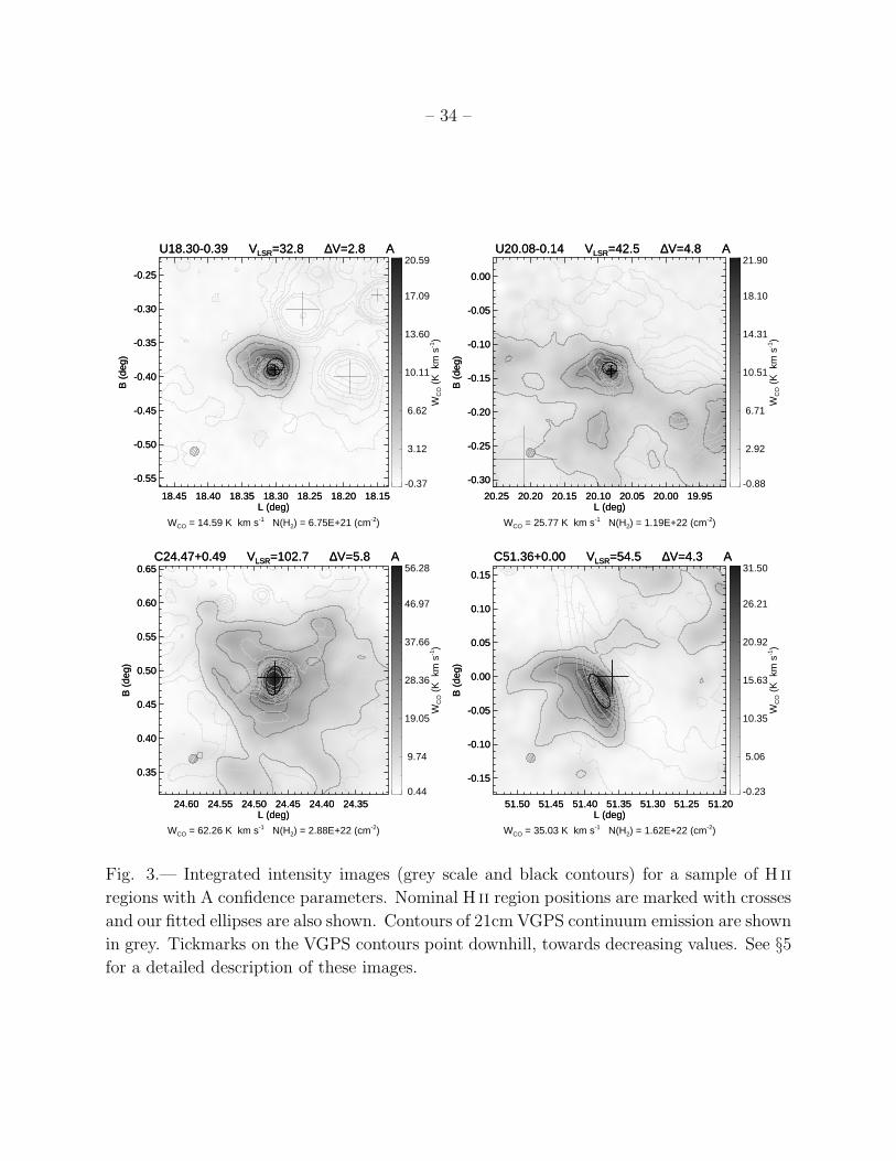
– 34 –

-0.37

3.12

6.62

10.11

13.60

17.09

20.59

WC

O (

K k

m s

-1)

U18.30-0.39 VLSR=32.8 ∆V=2.8 A

18.45 18.40 18.35 18.30 18.25 18.20 18.15L (deg)

-0.55

-0.50

-0.45

-0.40

-0.35

-0.30

-0.25

B (

deg)

U18.30-0.39 VLSR=32.8 ∆V=2.8 A

18.45 18.40 18.35 18.30 18.25 18.20 18.15L (deg)

-0.55

-0.50

-0.45

-0.40

-0.35

-0.30

-0.25

B (

deg)

WCO = 14.59 K km s-1 N(H2) = 6.75E+21 (cm-2)

-0.88

2.92

6.71

10.51

14.31

18.10

21.90

WC

O (

K k

m s

-1)

U20.08-0.14 VLSR=42.5 ∆V=4.8 A

20.25 20.20 20.15 20.10 20.05 20.00 19.95L (deg)

-0.30

-0.25

-0.20

-0.15

-0.10

-0.05

0.00

B (

deg)

U20.08-0.14 VLSR=42.5 ∆V=4.8 A

20.25 20.20 20.15 20.10 20.05 20.00 19.95L (deg)

-0.30

-0.25

-0.20

-0.15

-0.10

-0.05

0.00

B (

deg)

WCO = 25.77 K km s-1 N(H2) = 1.19E+22 (cm-2)

0.44

9.74

19.05

28.36

37.66

46.97

56.28

WC

O (

K k

m s

-1)

C24.47+0.49 VLSR=102.7 ∆V=5.8 A

24.60 24.55 24.50 24.45 24.40 24.35L (deg)

0.35

0.40

0.45

0.50

0.55

0.60

0.65

B (

deg)

C24.47+0.49 VLSR=102.7 ∆V=5.8 A

24.60 24.55 24.50 24.45 24.40 24.35L (deg)

0.35

0.40

0.45

0.50

0.55

0.60

0.65

B (

deg)

WCO = 62.26 K km s-1 N(H2) = 2.88E+22 (cm-2)

-0.23

5.06

10.35

15.63

20.92

26.21

31.50

WC

O (

K k

m s

-1)

C51.36+0.00 VLSR=54.5 ∆V=4.3 A

51.50 51.45 51.40 51.35 51.30 51.25 51.20L (deg)

-0.15

-0.10

-0.05

0.00

0.05

0.10

0.15

B (

deg)

C51.36+0.00 VLSR=54.5 ∆V=4.3 A

51.50 51.45 51.40 51.35 51.30 51.25 51.20L (deg)

-0.15

-0.10

-0.05

0.00

0.05

0.10

0.15

B (

deg)

WCO = 35.03 K km s-1 N(H2) = 1.62E+22 (cm-2)

Fig. 3.— Integrated intensity images (grey scale and black contours) for a sample of H ii

regions with A confidence parameters. Nominal H ii region positions are marked with crosses

and our fitted ellipses are also shown. Contours of 21cm VGPS continuum emission are shown

in grey. Tickmarks on the VGPS contours point downhill, towards decreasing values. See §5for a detailed description of these images.

– 35 –

-0.19

3.97

8.13

12.29

16.45

20.61

24.78

WC

O (

K k

m s

-1)

C18.95-0.02 VLSR=44.6 ∆V=4.1 B

19.10 19.05 19.00 18.95 18.90 18.85 18.80L (deg)

-0.15

-0.10

-0.05

0.00

0.05

0.10

B (

deg)

C18.95-0.02 VLSR=44.6 ∆V=4.1 B

19.10 19.05 19.00 18.95 18.90 18.85 18.80L (deg)

-0.15

-0.10

-0.05

0.00

0.05

0.10

B (

deg)

WCO = 20.61 K km s-1 N(H2) = 9.52E+21 (cm-2)

-0.10

3.74

7.58

11.42

15.27

19.11

22.95

WC

O (

K k

m s

-1)

U27.19-0.08b VLSR=93.4 ∆V=3.3 B

27.35 27.30 27.25 27.20 27.15 27.10 27.05L (deg)

-0.25

-0.20

-0.15

-0.10

-0.05

0.00

0.05

B (

deg)

U27.19-0.08b VLSR=93.4 ∆V=3.3 B

27.35 27.30 27.25 27.20 27.15 27.10 27.05L (deg)

-0.25

-0.20

-0.15

-0.10

-0.05

0.00

0.05

B (

deg)

WCO = 11.71 K km s-1 N(H2) = 5.41E+21 (cm-2)

1.15

4.83

8.50

12.18

15.85

19.53

23.21

WC

O (

K k

m s

-1)

D28.00-0.03 VLSR=98.8 ∆V=6.4 B

28.15 28.10 28.05 28.00 27.95 27.90 27.85L (deg)

-0.15

-0.10

-0.05

0.00

0.05

0.10

B (

deg)

D28.00-0.03 VLSR=98.8 ∆V=6.4 B

28.15 28.10 28.05 28.00 27.95 27.90 27.85L (deg)

-0.15

-0.10

-0.05

0.00

0.05

0.10

B (

deg)

WCO = 17.75 K km s-1 N(H2) = 8.21E+21 (cm-2)

-0.57

10.95

22.47

33.98

45.50

57.02

68.54

WC

O (

K k

m s

-1)

C49.44-0.47 VLSR=57.5 ∆V=3.8 B

49.60 49.55 49.50 49.45 49.40 49.35 49.30L (deg)

-0.60

-0.55

-0.50

-0.45

-0.40

-0.35

B (

deg)

C49.44-0.47 VLSR=57.5 ∆V=3.8 B

49.60 49.55 49.50 49.45 49.40 49.35 49.30L (deg)

-0.60

-0.55

-0.50

-0.45

-0.40

-0.35

B (

deg)

WCO = 30.04 K km s-1 N(H2) = 1.39E+22 (cm-2)

Fig. 4.— Integrated intensity images for a sample of H ii regions with B confidence param-

eters. Other parameters are as in Figure 3.

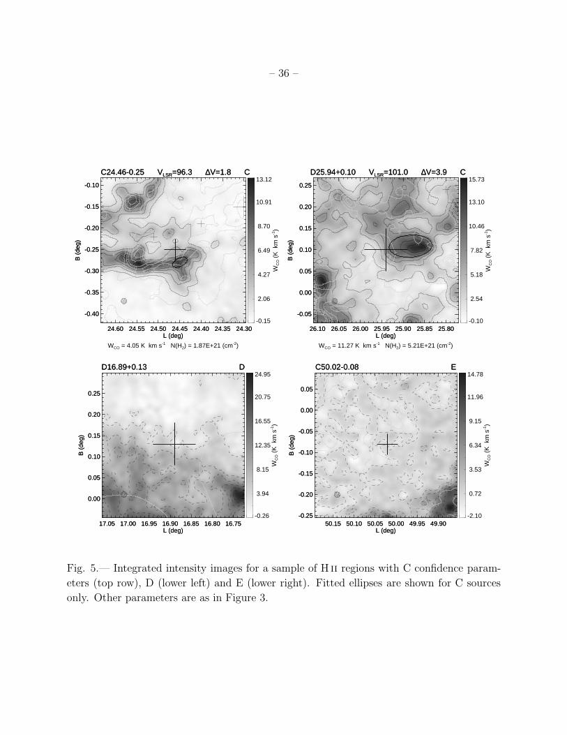
– 36 –

-0.15

2.06

4.27

6.49

8.70

10.91

13.12

WC

O (

K k

m s

-1)

C24.46-0.25 VLSR=96.3 ∆V=1.8 C

24.60 24.55 24.50 24.45 24.40 24.35 24.30L (deg)

-0.40

-0.35

-0.30

-0.25

-0.20

-0.15

-0.10

B (

deg)

C24.46-0.25 VLSR=96.3 ∆V=1.8 C

24.60 24.55 24.50 24.45 24.40 24.35 24.30L (deg)

-0.40

-0.35

-0.30

-0.25

-0.20

-0.15

-0.10

B (

deg)

WCO = 4.05 K km s-1 N(H2) = 1.87E+21 (cm-2)

-0.10

2.54

5.18

7.82

10.46

13.10

15.73

WC

O (

K k

m s

-1)

D25.94+0.10 VLSR=101.0 ∆V=3.9 C

26.10 26.05 26.00 25.95 25.90 25.85 25.80L (deg)

-0.05

0.00

0.05

0.10

0.15

0.20

0.25

B (

deg)

D25.94+0.10 VLSR=101.0 ∆V=3.9 C

26.10 26.05 26.00 25.95 25.90 25.85 25.80L (deg)

-0.05

0.00

0.05

0.10

0.15

0.20

0.25

B (

deg)

WCO = 11.27 K km s-1 N(H2) = 5.21E+21 (cm-2)

-0.26

3.94

8.15

12.35

16.55

20.75

24.95

WC

O (

K k

m s

-1)

D16.89+0.13 D

17.05 17.00 16.95 16.90 16.85 16.80 16.75L (deg)

0.00

0.05

0.10

0.15

0.20

0.25

B (

deg)

D16.89+0.13 D

17.05 17.00 16.95 16.90 16.85 16.80 16.75L (deg)

0.00

0.05

0.10

0.15

0.20

0.25

B (

deg)

-2.10

0.72

3.53

6.34

9.15

11.96

14.78

WC

O (

K k

m s

-1)

C50.02-0.08 E

50.15 50.10 50.05 50.00 49.95 49.90L (deg)

-0.25

-0.20

-0.15

-0.10

-0.05

0.00

0.05

B (

deg)

C50.02-0.08 E

50.15 50.10 50.05 50.00 49.95 49.90L (deg)

-0.25

-0.20

-0.15

-0.10

-0.05

0.00

0.05

B (

deg)

Fig. 5.— Integrated intensity images for a sample of H ii regions with C confidence param-

eters (top row), D (lower left) and E (lower right). Fitted ellipses are shown for C sources

only. Other parameters are as in Figure 3.

– 37 –

All UC

CompactDiffuse

0

20

40

60

80

100

120

0

20

40

60

80

0

10

20

30

A B C D E

0

5

10

15

20

25

A B C D E

Confidence Parameter

Num

ber

of S

ourc

es

Fig. 6.— The number distributions of the qualitative confidence parameter, CP . Sources

with associated molecular gas are rated A, B or C in order of decreasing confidence in the

association (see §5 text). Confidence parameter D and E sources have little or no associated

molecular emission, respectively. The top left panel is a stacked histogram where the top

line shows the histogram for the entire sample of 301 H ii regions. The open, hatched and

grey histograms show the contribution that UC, Compact, and Diffuse nebulae, respectively,

make to the total in each bin.

– 38 –

0 20 40 60 80 100 120Vlsr (km/s)

20

30

40

50

Gal

actic

Lon

gitu

de (

deg)

Fig. 7.— Longitude-LSR velocity diagram for 253 H ii regions in our sample that show

associated 13CO emission. Symbols indicate the confidence parameter of each nebula: CP

A (large filled circles), B (small filled circles), or C (small open circles). The lines show

the locii of the LSR terminal velocity expected from two different Galactic rotation curve

models: Clemens (1985) (dotted line) and Brand (1986) (full line).

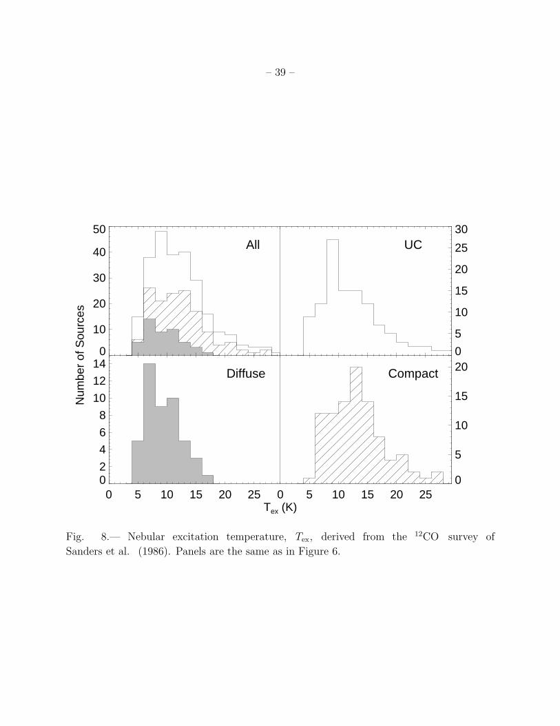
– 39 –

All UC

CompactDiffuse

0

10

20

30

40

50

0

5

10

15

20

25

30

0

5

10

15

20

0 5 10 15 20 25

02

4

6

8

10

12

14

0 5 10 15 20 25

Tex (K)

Num

ber

of S

ourc

es

Fig. 8.— Nebular excitation temperature, Tex, derived from the 12CO survey of

Sanders et al. (1986). Panels are the same as in Figure 6.

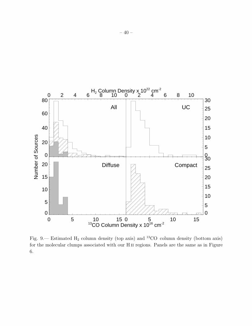
– 40 –

All UC

CompactDiffuse

0

20

40

60

80

0

5

10

15

20

25

30

0

5

10

15

20

25

30

0 5 10 15

0

5

10

15

20

0 5 10 15

13CO Column Density x 1016 cm-2

Num

ber

of S

ourc

es

H2 Column Density x 1022 cm-2

0 2 4 6 8 10 0 2 4 6 8 10

Fig. 9.— Estimated H2 column density (top axis) and 13CO column density (bottom axis)

for the molecular clumps associated with our H ii regions. Panels are the same as in Figure

6.

– 41 –

All UC

CompactDiffuse

05

10

15

20

25

3035

02

4

6

8

10

1214

02

4

6

8

10

12

-10 -5 0 5 10

0

2

4

6

8

-10 -5 0 5 10

VCO - VRRL (km s-1)

Num

ber

of S

ourc

es

Fig. 10.— The LSR velocity difference between the H ii region RRL and molecular gas 13CO

velocity. The distribution peaks near zero, as expected. Panels are the same as in Figure 6.

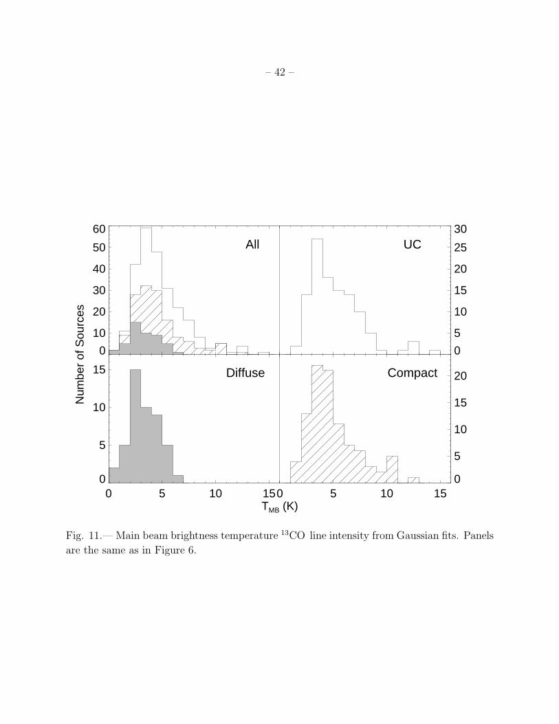
– 42 –

All UC

CompactDiffuse

0

10

20

30

40

50

60

0

5

10

15

20

25

30

0

5

10

15

20

0 5 10 15

0

5

10

15

0 5 10 15

TMB (K)

Num

ber

of S

ourc

es

Fig. 11.— Main beam brightness temperature 13CO line intensity from Gaussian fits. Panels

are the same as in Figure 6.

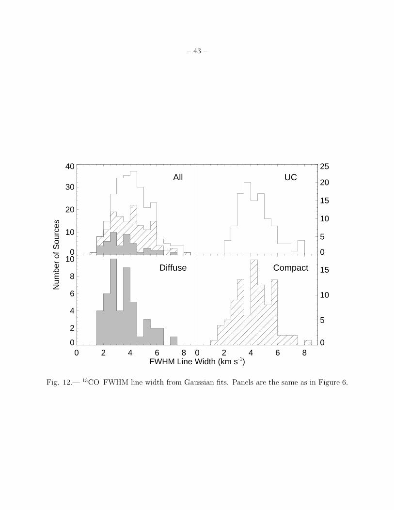
– 43 –

All UC

CompactDiffuse

0

10

20

30

40

0

5

10

15

20

25

0

5

10

15

0 2 4 6 8

0

2

4

6

8

10

0 2 4 6 8

FWHM Line Width (km s-1)

Num

ber

of S

ourc

es

Fig. 12.— 13CO FWHM line width from Gaussian fits. Panels are the same as in Figure 6.

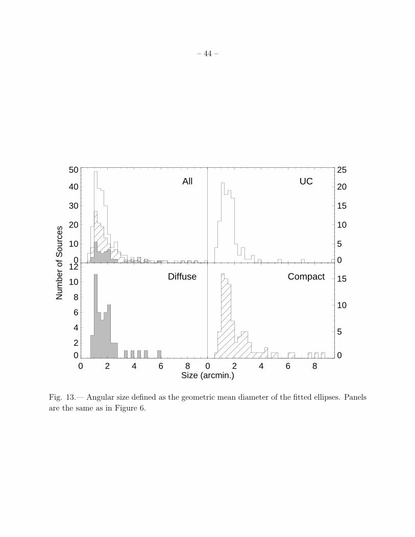
– 44 –

All UC

CompactDiffuse

0

10

20

30

40

50

0

5

10

15

20

25

0

5

10

15

0 2 4 6 8

02

4

6

8

10

12

0 2 4 6 8

Size (arcmin.)

Num

ber

of S

ourc

es

Fig. 13.— Angular size defined as the geometric mean diameter of the fitted ellipses. Panels

are the same as in Figure 6.

– 45 –

0 2 4 6 8FWHM Line Width (km s-1)

0

5

10

15

TM

B (

K)

Fig. 14.— 13CO line intensity plotted as a function of FWHM line width. Shown are

all the CP A, B, or C sources: UC (filled triangles), Compact (filled circles), and Diffuse

(open squares) nebulae. The lines dividing the figure into quadrants are from an analysis of

molecular clumps in the GRS dataset (see §5.2).