Regional Patterns of Erosion and Sediment Transport in the Burdekin ... - Land and Water · 2005-10-14 · Regional Patterns of Erosion and Sediment Transport in the Burdekin River

C S I R O L A N D a nd WAT E R

Regional Patterns of Erosion and Sediment Transport

in the Burdekin River Catchment

I.P. Prosser, C.J. Moran, H.Lu, A. Scott, P. Rustomji, J. Stevenson,

G. Priestly, C.H. Roth and D. Post

CSIRO Land and Water

Technical Report 5/02, February 2002

Regional Patterns of Erosion and Sediment Transport

in the Burdekin River Catchment

I.P. Prosser, C.J. Moran, H.Lu, A. Scott, P. Rustomji, J. Stevenson,

G. Priestly, C.H. Roth and D. Post

CSIRO Land and Water

Technical Report 5/02, February 2002

Copyright© 2001 CSIRO Land and Water.

To the extent permitted by law, all rights are reserved and no part of this publication covered bycopyright may be reproduced or copied in any form or by any means except with the writtenpermission of CSIRO Land and Water.

Important Disclaimer

To the extent permitted by law, CSIRO Land and Water (including its employees and consultants)excludes all liability to any person for any consequences, including but not limited to all losses,damages, costs, expenses and any other compensation, arising directly or indirectly from usingthis publication (in part or in whole) and any information or material contained in it.

ISBN 0 643 061002

1

Table of Contents

Abstract ......................................................................................................................................................................... 4Executive Summary ...................................................................................................................................................... 4Main Research Report................................................................................................................................................... 5

Background ............................................................................................................................................................... 5Project Objectives ..................................................................................................................................................... 8Methods .................................................................................................................................................................... 8

Hillslope Erosion Hazard ...................................................................................................................................... 9Gully Erosion Hazard.......................................................................................................................................... 10Sediment Delivery Through the River Network ................................................................................................. 11Contribution of Sediment to the Coast ................................................................................................................ 15Suspended Sediment Budget Under Natural Conditions..................................................................................... 15Hydrology ........................................................................................................................................................... 16

Results and Discussion............................................................................................................................................ 16Hillslope Erosion Hazard .................................................................................................................................... 16Gully Erosion Hazard.......................................................................................................................................... 21Streambank Erosion ............................................................................................................................................ 26Sediment Sources to the Stream Network........................................................................................................... 27Sediment Delivery Through the River Network ................................................................................................. 30Bedload Deposition............................................................................................................................................. 32River Suspended Loads....................................................................................................................................... 32Contribution to Sediment Export at the Coast..................................................................................................... 37Summary Plots and Calibration of Suspended Sediment Load........................................................................... 39Improvements Required ...................................................................................................................................... 41

Conclusions............................................................................................................................................................. 41References............................................................................................................................................................... 42

2

List of Figures (abbreviated titles)

Figure 1: A river network showing links, nodes, Shreve magnitude of each link, and internal catchmentarea……………………………………………………………………………………………………12

Figure 2: Conceptual diagram of the bedload sediment budget for a river link.. ...................................13Figure 3: Conceptual diagram for the suspended sediment budget of a river link. ...............................14Figure 4: Location map for the Burdekin River catchment.....................................................................17Figure 5: Map showing mean annual rainfall for the Burdekin River catchment and river names. .......18Figure 6: Predicted hillslope erosion hazard in the Burdekin River catchment for each 9" cell.............19Figure 7: Monthly distribution of total soil loss within the Burdekin River catchment ............................21Figure 8: Maps of RUSLE factors that contribute to Figure 6. ...............................................................22Figure 9: Pre-European hillslope erosion rate and ratio of current to Pre-European results.................23Figure 10: Predicted density of gully erosion based on 1.25 km pixels. ..................................................25Figure 11: Mean gully density classified by major geology class ...........................................................26Figure 12: Predicted amount of intact riparian vegetation. ......................................................................28Figure 13: Ratio of hill to gully and bank erosion. ....................................................................................29Figure 14: Regionalisation of the discharge term of streampower (ΣQ1.4) with catchment area. ............31Figure 15: Relationship of river channel width with catchment area........................................................31Figure 16: Predicted sediment transport capacity....................................................................................33Figure 17: Predicted bedload deposition..................................................................................................34Figure 18: Predicted floodplain width. ......................................................................................................35Figure 19: Predicted suspended sediment load.......................................................................................36Figure 20: Predicted contribution of suspended sediment to the coast ...................................................38Figure 21: Summary of predicted suspended sediment yield across the Burdekin catchment ...............40Figure 22: Sediment yield data for Australian catchments compiled by Wasson (1994).........................40

List of Photos (abbreviated titles)

Photo 1: Erosion gully in the Fanning River sub-catchment of the Burdekin River......................................6Photo 2: The Burdekin River at the Flinders Highway. ................................................................................7Photo 3: A tributary of the Burdekin River at low flow ..................................................................................8

List of Tables (abbreviated titles)

Table 1: Hillslope soil loss from land use categories in the Burdekin River catchment. ...........................20Table 2: Best achieved statistical figures of gully density model generated by CUBIST software ...........24Table 3: Components of the sediment budget. ..........................................................................................27

3

ACKNOWLEDGEMENT

This study was part of a larger Meat and Livestock Australia (MLA) funded collaboration with CSIRO/DPIinvestigating the effects of grazing on sediment and nutrient exports from the Burdekin Catchment. At the same timewe were able to draw on some of the innovative methodologies developed as a part of the National Land and WaterResources Audit (NLWRA) to determine sediment and nutrient export from Australia’s coastal catchments.

We gratefully acknowledge the funding support provided by MLA and NLWRA that made this study possible.

4

ABSTRACTThis project was carried out to identify the major processes involved in the delivery of sediment andnutrients to rivers within the Burdekin River catchment. It has identified critical areas of erosion potential,the physical processes that dominate in these areas and which areas are the major contributors ofsediment and nutrients to the coast. The project outcomes will be of benefit to the grazing industry andother natural resource management agencies, enabling them to target these critical areas and thus toeffectively use the resources directed at minimizing sediment and nutrient export from grazed land.

EXECUTIVE SUMMARYThe loss of sediment and nutrients from the land can have impacts downstream on the river and themarine environments that receive this material. In low input farming systems such as the northern beefindustry, the bulk of nutrients, phosphorus and nitrogen, are transported with sediment. An essential partof minimizing the impact of sediment is to reduce losses from the landscape. In large regionalcatchments, such as the Burdekin River, there are a wide range of environments only some of which willcontribute significant amounts of sediment to streams. There are also many opportunities for depositionof sediment in the catchment so that not all areas of erosion result in export of sediment from thecatchment.

The aim of this report is to identify sediment sources in the Burdekin River catchment by identifying thedominant processes and the sub-catchments that have high erosion potential. The project also looks atpatterns of sediment transport through the river network, identifying which reaches may be impacted bydeposition of sand on river beds, and which sub-catchments contribute the most to suspended sedimentloads and export from the river basin. We address these issues by constructing a sediment budget forthe catchment. A sediment budget is an account of the major sources, stores and fluxes of sediment inthe catchment.

Spatial modeling is the only practical method to assess the patterns of sediment transport in a largecomplex catchment as there are only limited measurements of sediment transport rates. Modelling canbe used to interpolate these measurements and combine them with a basic understanding of transportprocesses and geographical information on controlling factors. This includes mapping of soils, vegetationcover, geology, terrain, climate and measurements of river discharge. We produce maps and summarystatistics of predicted surface wash erosion, gully erosion, riverbank erosion and bedload and suspendedload transport across the catchment.

The model results suggest that surface erosion varies by three orders of magnitude across thecatchment. Only 25 % of the catchment has high surface wash erosion potential. Much of this is in theBowen River sub-catchment, the area below the Burdekin Falls Dam and parts of the Upper Burdekincatchment. The Suttor and Belyando River catchments have low surface wash erosion potential.

Gully erosion is also a significant process contributing approximately 30% of the total predicted sedimentload carried by streams. We predict it to be most pronounced in granitic and ancient sedimentarylandscapes in the central part of the catchment. Gully and streambank erosion are the dominantsediment sources in the drier parts of the catchment where delivery of sediment to streams from surfacewash erosion is low.

The sediment budget predicts that only 16% of suspended sediment and 4% of bedload delivered to theriver network in any year is exported from the river mouth. The rest is stored within floodplains, as sandand gravel deposits on the bed of streams, and in reservoirs. This is typical of large river systems andmuch of the sediment remains stored for hundreds to thousands of years. We predict that the meanannual export of suspended sediment to the coast is 2.4 Mt/y. This conforms with monitoring of sedimentloads in the lower river. Rapid accumulation of sand and gravel on the bed of rivers can degrade aquatichabitat, but we find that this is not a major concern in the Burdekin River catchment. Most river reachesare capable of transporting increases in supply of bedload from gully and riverbank erosion. Only in thearea around the Burdekin Falls Dam and parts of the Bowen River catchment do we predict significantaccumulation of sand and gravel.

5

Much of the suspended sediment load of the Burdekin River basin is generated from the Upper Burdekincatchment and the Bowen River catchment because of both high erosion rates and low amounts ofdeposition on floodplains in those areas. The Suttor and Belyando Rivers contribute relatively littlesuspended sediment because of extensive lowland floodplains and lower sediment supply to streams.Much of the catchment contributes very little to sediment export to the coast because of the long traveldistances with many opportunities for deposition along the way, or because of low rates of sedimentsupply to the stream. We predict that 90% of the sediment delivered to the Burdekin Falls Dam is trappedby the dam. This results in approximately 95% of the sediment export to the coast being generated fromjust 13% of the catchment area. Overall the dominant sources are the sub-catchments downstream ofthe Burdekin Falls Dam, the Bowen River, and parts of the Upper Burdekin catchment. Grazing landscontribute 85% of this load simply because of the vast areas of grazing land within the catchment,occupying 90% of land in the catchment. The majority of grazing land, particularly in the drier parts of thecatchment contributes little sediment to the coast.

The results from this project demonstrate that an assessment tool for constructing sediment budgetsacross a complex catchment, such as the one applied here, has strong potential for guiding furtherinvestigation, identifying areas for improved management and for setting targets of catchment restoration.Significantly, the results predict that erosion processes are highly focused, with much of the sedimentbeing generated from relatively small areas. If future efforts at minimising soil loss are targeted towardsthese hotspots, using refined grazing management guidelines, a comparatively large benefit in reducedsediment loads downstream can be achieved with less effort. The targeted restoration (to be developedthrough further work in the project) need to be specially adapted to the particular soil and pasturecommunities prevalent in those sub-catchments or landscapes identified as hotspots. They also need tobe differentiated to specifically address hillslope or gully erosion, whichever is the more important form oferosion in a particular area. The project results predict that each erosion process (surface wash, gullyerosion, riverbank erosion) is significant in particular locations. Outputs from this research componentshould therefore assist the grazing industry, extension providers, and natural resource managementagencies to appropriately target critical areas and as a consequence maximise resources directed atminimising sediment and nutrient export from grazed land. The project has also resulted in methods thatcan now be applied more readily to resource management issues in other catchments.

MAIN RESEARCH REPORTBackgroundA significant aspect of achieving an ecologically sustainable beef industry is to ensure that thedownstream impacts of grazing on streams are minimised. An essential part of minimising impact is toreduce the delivery of sediments and nutrients from land to streams. For low input farming systems suchas extensive beef grazing, the bulk of the nutrient load is transported attached to sediment so thatsediment and nutrient transport are intimately linked.

To put pastoral land use in the context of the regional catchments in which it occurs requires us toconceptualise the critical sources, transport pathways and sinks of sediment and nutrient in a catchment.We need to identify where sediment and nutrient is derived from, where it is stored within the catchment,and how much is delivered downstream to rivers and the sea. To quantify sources, stores and delivery isto construct a sediment budget for a catchment or any part of a catchment. This is a critical step toconceptualise the context of land use in a large regional catchment and to focus more detailed studies onthe areas of greatest potential impact. Few studies of regional sediment and nutrient budgets have beenconducted, and none to date pertain to the north Australian beef industry.

Grazed catchments such as the Burdekin are complex systems, often with considerable variation ingrazing pressure, and diverse topography, soils, rainfall and vegetation cover. Thus before changinggrazing management or even undertaking remediation measures we need to determine its significanceand the spatial pattern of grazing impact for sediment and nutrient transport. We also need to put themore detailed investigations of other parts of this project in a broader regional environmental context forthe results to be applicable across wider areas.

6

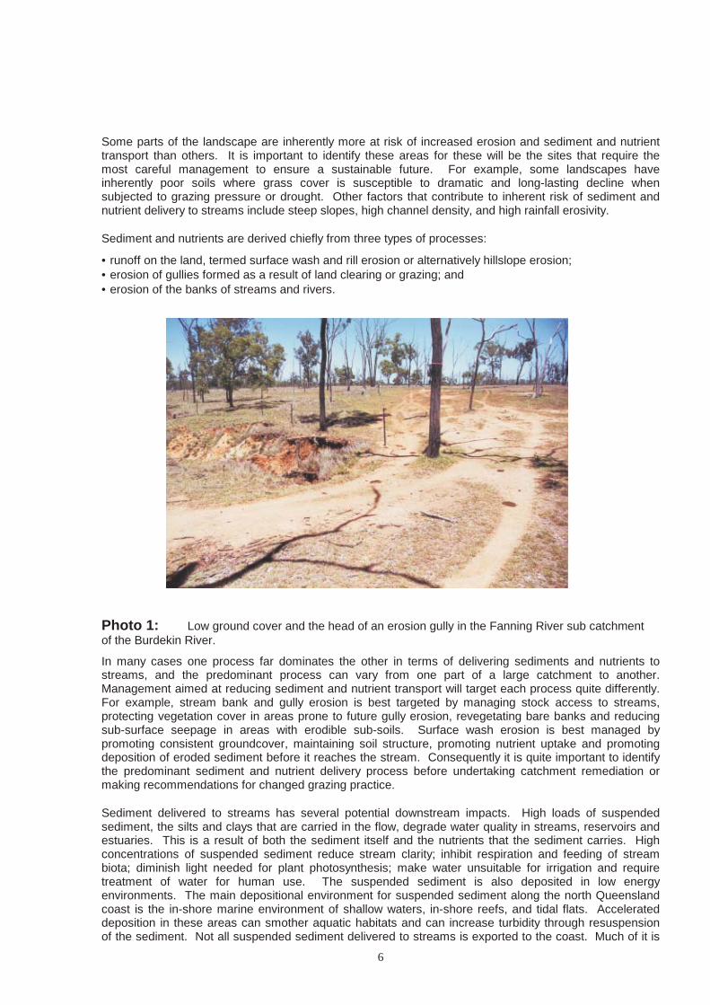
Some parts of the landscape are inherently more at risk of increased erosion and sediment and nutrienttransport than others. It is important to identify these areas for these will be the sites that require themost careful management to ensure a sustainable future. For example, some landscapes haveinherently poor soils where grass cover is susceptible to dramatic and long-lasting decline whensubjected to grazing pressure or drought. Other factors that contribute to inherent risk of sediment andnutrient delivery to streams include steep slopes, high channel density, and high rainfall erosivity.

Sediment and nutrients are derived chiefly from three types of processes:

• runoff on the land, termed surface wash and rill erosion or alternatively hillslope erosion;• erosion of gullies formed as a result of land clearing or grazing; and• erosion of the banks of streams and rivers.

Photo 1: Low ground cover and the head of an erosion gully in the Fanning River sub catchmentof the Burdekin River.

In many cases one process far dominates the other in terms of delivering sediments and nutrients tostreams, and the predominant process can vary from one part of a large catchment to another.Management aimed at reducing sediment and nutrient transport will target each process quite differently.For example, stream bank and gully erosion is best targeted by managing stock access to streams,protecting vegetation cover in areas prone to future gully erosion, revegetating bare banks and reducingsub-surface seepage in areas with erodible sub-soils. Surface wash erosion is best managed bypromoting consistent groundcover, maintaining soil structure, promoting nutrient uptake and promotingdeposition of eroded sediment before it reaches the stream. Consequently it is quite important to identifythe predominant sediment and nutrient delivery process before undertaking catchment remediation ormaking recommendations for changed grazing practice.

Sediment delivered to streams has several potential downstream impacts. High loads of suspendedsediment, the silts and clays that are carried in the flow, degrade water quality in streams, reservoirs andestuaries. This is a result of both the sediment itself and the nutrients that the sediment carries. Highconcentrations of suspended sediment reduce stream clarity; inhibit respiration and feeding of streambiota; diminish light needed for plant photosynthesis; make water unsuitable for irrigation and requiretreatment of water for human use. The suspended sediment is also deposited in low energyenvironments. The main depositional environment for suspended sediment along the north Queenslandcoast is the in-shore marine environment of shallow waters, in-shore reefs, and tidal flats. Accelerateddeposition in these areas can smother aquatic habitats and can increase turbidity through resuspensionof the sediment. Not all suspended sediment delivered to streams is exported to the coast. Much of it is

7

deposited along the way on floodplains, providing fertile alluvial soils, or it is deposited in reservoirs. Theextent of this deposition is highly variable from one river reach to another. Deposition potential must beconsidered when trying to relate catchment land use to downstream loads of sediment.

Photo 2: The Burdekin River at the Flinders Highway showing suspended load carried in thewater and bedload deposits of sand and gravel.

The formation of gullies and accelerated erosion of stream banks can supply large amounts of sand andgravel to streams. These are transported as bedload, being rolled, and bounced along the bed ofstreams. Where streams are unable to transmit the load of sand and gravel downstream, it is deposited,burying the bed, and in extreme examples forming sheets of sand referred to as sand slugs (Rutherfurd,2000). Sand slugs are poor habitat. They can prevent fish passage, they fill pools and other refugia, andare unstable substrate for benthic organisms (Jeffers, 1998). Many semi-arid streams have natural bedsof sand, however, so the presence of extensive sand deposits on the bed of these streams should not betaken as an indicator of degradation. In this project we assess whether changes to the supply of sandand gravel to streams are likely to have changed the composition of the bed of streams in the Burdekincatchment.

A reconnaissance level sediment budget for the Burdekin River catchment will provide an understandingof the critical processes of sediment and nutrient transport that can lead to downstream impact. It willplace the beef industry in an appropriate regional context of broader land use issues. The budget willalso identify sub-catchments with the greatest potential for downstream impact on aquatic ecosystems.These are the first steps toward better targeting of remedial and land conservation measures. Thesediment budget demonstrates how relatively simple reconnaissance techniques can be used in regionalpolicy development in relation to the beef industry. It provides producers with broad guidelines to identifythe conditions under which there could be significant downstream impact of sediment and nutrient.

8

Photo 3: A tributary of the Burdekin River at low flow showing extensive bed deposits of sand.These can be a natural feature of semi-arid rivers.

Project ObjectivesThis report constitutes the final report for one of four research components (R1) of the MLA/CSIRO/QDPIproject “Reducing Sediment and Nutrient Export From Grazed Land in the Burdekin Catchment forSustainable Beef Production”. The specific objectives of the component are:

• To survey the Burdekin catchment at a reconnaissance scale to identify crucial sub-catchmentsappropriate for more detailed investigation;

• to assess the most significant processes of soil erosion as they relate to grazing management; and

• to provide a framework for reviewing and integrating information currently available in the catchment.

MethodsThe only practical framework to assess the patterns of sediment and nutrient transport across a largecomplex area such as the Burdekin River catchment is a spatial modelling framework. There are fewdirect measurements of sediment transport in regional catchments, and it is unrealistic to initiate samplingprograms of the processes now and expect results within a decade. Furthermore, collation andintegration of existing data has to be put within an overall assessment framework, and a large-scalespatial model of sediment transport is the most effective use of that data.

The assessment of sediment transport is divided into three aspects: hillslope erosion as a source ofsediment; gully erosion as a source of sediment; and river links as a further source, receiver andpropagator of the sediment. The methods used in each aspect of the spatial model are outlined below inbrief. They were developed concurrently with a National Land and Water Resources Audit project onsediment budgets and reference is made to supporting technical documentation which contains details ofthe approach.

9

Hillslope Erosion Hazard

The controls on hillslope erosion by surface wash and rill erosion are well understood and there areseveral models which incorporate these factors. The best known model and the only one that can beapplied across large regions is the Universal Soil Loss Equation (USLE; Wischmeier and Smith, 1978)and its derivatives such as the Revised USLE (RUSLE; Renard et al., 1997), Soiloss (USLE factors forNSW; Rosewell, 1993) and PERFECT (Littleboy et al., 1992). Research on the processes of hillslopeerosion has resulted in more detailed models of the mechanics of sediment detachment and transport butthese cannot be used at regional scales because they require parameters which are unavailable beyondlimited experimental conditions. Support for the USLE is given by studies which show that its empiricalform is consistent with the mechanics of sediment detachment and transport included in the more detailedmodels (Moore and Burch, 1986; McCool et al., 1989).

The RUSLE calculates mean annual soil loss (Y, tonnes/ha/y) as a product of six factors: rainfall erosivityfactor (R), soil erodibility factor (K), hillslope length factor (L), hillslope gradient factor (S), ground coverfactor (C) and land use practice factor (P):

Y = RKLSCP(1)

The factors included in the RUSLE vary strongly across a diverse catchment such as the Burdekin,providing a method for estimating the spatial patterns of erosion using available spatial information foreach factor.

The precise form of each factor is based on soil loss measurements on hillslope plots, mainly in the USA.Plot scale measurements of erosion have been undertaken in the Burdekin area (McIvor et al., 1995;Scanlan et al., 1996) allowing limited local calibration of the RUSLE factors, particularly the C factor.

The RUSLE is directly applicable for hillslopes up to 300 m in length. For longer hillslopes we canextrapolate the relationship based on expected runoff patterns on longer hillslopes. The L factorrepresents the increase in storm runoff volume with increasing hillslope length, and the increasedpropensity for rill erosion with increasing runoff. In native grasslands, woodlands and forests there isevidence that runoff volume grows only weakly or not at all with hillslope length (Bonell and Williams,1987; Prosser and Williams, 1998). In these landscapes there are patches of runoff generation andpatches of runoff adsorption and longer hillslopes do not necessarily yield more sediment than shortones. Thus the L factor was removed from the analysis in these areas and only applied to areas withcropping or improved pastures. Similarly, there are few land use practises such as tillage andconstruction of contour banks in extensive savannah grazing lands so the P factor was also removedfrom the spatial analysis.

Mean annual values for rainfall erosivity and the cover factor are often used in direct application ofEquation (1) to calculate mean annual hillslope erosion. This neglects often important seasonal patternsof rainfall erosivity and cover. High intensity rains for example may be associated with seasons of lowground cover. To incorporate these effects we used the product of mean monthly cover (Cm) and theproportion of annual rainfall erosivity for each month (Rm/R). The monthly values of CmRm/R were thensummed to give mean annual soil loss. It can be shown that incorporation of seasonal effects reducespredicted mean annual soil loss in Australia's tropics by a factor of 1.5. The modifications of Equation (1)discussed above yield

R

RCKLSY m

m

mm∑

=

==

12

1. (2)

Twenty years (1980-1999) of daily rainfall data mapped across Australia and 13 years (1981-1994) ofsatellite vegetation data were used to apply Equation (2). Details of the use of this data are given in Lu etal. (2001). The soil erodibility factor (K) was derived from the Australian Soil Resources InformationSystem (as detailed in Lu et al., 2001). The length and slope factors (L, S) were derived from the national9" digital elevation model (DEM; approximately 250 m grid resolution) and scaling rules were determinedfrom comparison with higher resolution DEMs (see Gallant, 2001 for details). This transformation was

10

needed because the raw values in the 9" DEM do not accurately reflect the topographic details ofhillslopes and valleys which are at a similar or finer scale than the resolution of the DEM.

The predictions of surface wash erosion under present land use need to be put in context of erosionunder natural vegetation cover, for many areas have naturally high surface wash erosion. We predictednatural erosion using the same procedure as above, using a cover factor for native vegetation andkeeping the other factors of soil erodibility, rainfall erosivity and topography as for the present day.

The cover factor for native vegetation was obtained by assessing areas of reserve where nativevegetation cover is retained in each of Australia’s native vegetation zones. In the reserves, the RUSLE Cfactor was determined from remote sensing data as part of the assessment of current soil loss. Thenative vegetation cover of these reserve areas was extrapolated across other areas using an empiricaldecision tree model based on climatic, topographic, and geological factors. The acceleration of currentmean annual soil loss above natural rates was predicted as the ratio of the current to pre-European meanannual soil loss predictions. Further details are given in Lu et al. (2001).

Gully Erosion Hazard

As it is an expensive and time consuming effort to measure all the gullies within the Burdekin catchment,the extent of gullies was estimated by aerial photograph interpretation of a number of sampled areas.These were used to generate an empirical model of gully density based on various environmentalattributes for which there is catchment-wide coverage.

Sample sites were selected in each of the major geology types, slopes and rainfall zones. To ensuresatisfactory representation of the different terrains, each major land system is represented by a number ofphotographs, and the photographs covered all geographical areas of the catchment. There is however, abias towards the central part of the catchment since suitable air photos were more readily available forthis region. A total of 63 pairs of photos were used. Eroded gullies were mapped from the aerialphotographs using a stereoscope and then scanned and digitised into a geographical information system(GIS). Each image was then geo-referenced using 5 to 6 control points, which were obtained from1:100,000 topographic maps. For each air photo, the mapped gullies were grouped into areas (orpolygons) of similar geology, land-use and slope. Each aerial photograph was then divided into blocks ofsimilar terrain based upon land use, geology and relief. Each region, thus delineated, is allocated thegully density (km of eroded gully per km2 of area) measured across that whole region. The gully density isthen calculated by dividing the total length of gully by the area of the polygon, to give a value in km oferoded gully per km2 of area.

For building a spatial model of gully density a grid resolution of 1.25 km was selected. We consider thisto be the smallest scale at which gully prediction is feasible using the variables available. It is also theapproximate scale at which the original aerial photograph interpretation was done. The gully erosionmodel was built using 75% of pixels for which there was aerial photograph interpreted gully density. Thepredictor environmental variables were also sampled over the same locations. These included climaticparameters such as mean annual rainfall; various soil attributes derived from the Atlas of Australian Soilsand McKenzie et al. (2000); geology; land use; and terrain attributes derived from the 9" DEM. A numberof training sets were used by varying the random sampling of pixel locations, and by varying the predictorvariables. This ensured that the model was not sensitive to the precise choice of measured sites, andused the best combination of predictor variables.

Sets of gully density rules were determined using the CUBIST decision tree software. This is a datamining tool for generating rule-based predictive models for large volumes of data. The basic modelbuilding methods of CUBIST can be found in Quinlan (1993). CUBIST builds a model of gully erosionbased on piece-wise linear multiple regression of the predictor variables. The remaining 25% ofmeasured gully pixels were used to test the quality of the model. The best model was selected on thebasis of the highest correlation coefficient, smallest absolute and relative error, and consistent statisticalfigures between training set and testing set. Finally, a gully density map was produced by applying therules generated by the decision tree to the predictor variables mapped over the entire catchment.Hughes et al. (2001) contains further details of the method.

11

Sediment Delivery Through the River Network

Hillslope and gully erosion, together with erosion of streambanks, supply sediment to the stream network(the network of creeks and rivers in a catchment). The sediment supplied to a reach of river is then eitherdeposited within the river, and its surrounding floodplain, or is transmitted to the next reach downstream.There is also substantial deposition in reservoirs.

To calculate the supply of sediment, its deposition and its delivery downstream is to construct a riversediment budget. We calculated budgets for two types of sediment: suspended sediment and bedload.A suit of ArcInfoTM programs were used to define river networks and their sub-catchments; importrequired data; implement the model; and compile the results. The programs are referred to collectively asthe SedNet model: the Sediment River Network model. Details of the model and its application toregional catchments in Australia is given in Prosser et al. (2001). That document describes all theequations and input data used. Here we give a brief descriptive summary of the approach.

The SedNet model calculates, among other things:

• the mean annual suspended sediment output from each river link;

• the depth of sediment accumulated on the river bed in historical times;

• the relative supply of sediment from surface wash, gully and bank erosion processes;

• the mean annual rate of sediment accumulation in reservoirs;

• the mean annual export of sediment to the coast; and

• the contribution of each sub-catchment to that export.

For this project, suspended sediment is characterised as fine textured sediment carried at relativelyuniform concentration through the water column during large flows. The main process for net depositionof suspended sediment is overbank deposition on floodplains (e.g. Walling et al., 1992). The amount ofdeposition depends upon the residence time of water on the floodplain and the sediment concentration offlood flows. The residence time of suspended sediment in streams is low, so there is negligible transientdeposition of suspended sediment. Suspended sediment is sourced from surface wash erosion ofhillslopes, gully erosion and riverbank erosion. The sediment budget is reported as mean annual valuesfor either the current land use or for pre-European native vegetation cover.

Bedload is sediment transported in greatest proportions near the bed of a river. It may be transported byrolling, saltation, or for short periods of time, by suspension. Transport occurs during periods of high flow,over distances of hundreds to thousands of metres (Nicholas et al., 1995). Residence times of coarsesediment in river networks are relatively long so there is transient deposition on the bed as the sedimentworks its way through the river network. In addition to that deposition, an increase in sediment supplyfrom accelerated post-European erosion can cause the total supply of sediment in historical times toexceed the capacity of a river reach to transport sediment downstream. The excess sediment will bestored on the bed and the river will have aggraded over historical times (Trimble, 1981; Meade 1982).There has been a significant increase in supply of sand and fine gravel to rivers in historical times anddeposition of this bedload has formed sand slugs: extensive, flat sheets of sand deposited over previouslydiverse benthic habitat (Nicholas et al., 1995; Rutherfurd, 1996). The bedload budget aims to predict theformation of these sand slugs.

The basic unit of calculation for constructing the sediment budgets is a link in a river network. A link is thestretch of river between any two stream junctions (or nodes; Figure 1). Each link has an internal sub-catchment, from which sediment is delivered to the river network by hillslope and gully erosion processes.The internal catchment area is the catchment area added to the link between its upper and lower nodes(Figure 1). For the purpose of the model, the internal catchment area of first order streams is the entirecatchment area of the river link. Additional sediment is supplied from bank erosion along the link andfrom any tributaries to the link

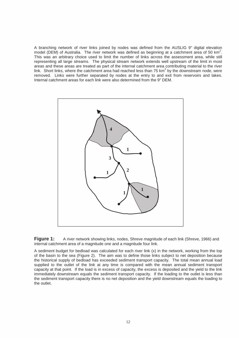
12

A branching network of river links joined by nodes was defined from the AUSLIG 9" digital elevationmodel (DEM) of Australia. The river network was defined as beginning at a catchment area of 50 km2.This was an arbitrary choice used to limit the number of links across the assessment area, while stillrepresenting all large streams. The physical stream network extends well upstream of the limit in mostareas and these areas are treated as part of the internal catchment area contributing material to the riverlink. Short links, where the catchment area had reached less than 75 km2 by the downstream node, wereremoved. Links were further separated by nodes at the entry to and exit from reservoirs and lakes.Internal catchment areas for each link were also determined from the 9" DEM.

Figure 1: A river network showing links, nodes, Shreve magnitude of each link (Shreve, 1966) andinternal catchment area of a magnitude one and a magnitude four link.

A sediment budget for bedload was calculated for each river link (x) in the network, working from the topof the basin to the sea (Figure 2). The aim was to define those links subject to net deposition becausethe historical supply of bedload has exceeded sediment transport capacity. The total mean annual loadsupplied to the outlet of the link at any time is compared with the mean annual sediment transportcapacity at that point. If the load is in excess of capacity, the excess is deposited and the yield to the linkimmediately downstream equals the sediment transport capacity. If the loading to the outlet is less thanthe sediment transport capacity there is no net deposition and the yield downstream equals the loading tothe outlet.

1

1

1

1

4

3

2

13

If loading < capacitycapacitycpacitycapacity• no deposition • yield = loading

Tributary supply (t/y)

Gully erosion (t/y)

Riverbank erosion (t/y)

Downstream yield (t/y)

STC (t/y)

If loading > capacity

• deposit excess • yield = capacity

Figure 2: Conceptual diagram of the bedload sediment budget for a river link. STC is the sedimenttransport capacity of the river link, determined by equation 3.

Bedload is supplied to a river link from tributary links and from gully and riverbank erosion in the internalcatchment area of the link. Half the sediment derived from riverbank and gully erosion contributed to thebedload budget and the other half contributed to the suspended load budget. This reflects observedsediment budgets (eg. Dietrich and Dunne, 1978) and particle size of the bank materials.

Mapping of gully erosion extent was described above. Gully density was converted to a mean annualmass of sediment derived from gully erosion by assuming development of gullies over 100 y and a meangully cross-sectional area of 10 m2.

The supply of sediment from riverbank erosion was calculated from the results of a global review of riverbank migration data (Rutherfurd, 2000). The best predictor of bank erosion rate was found to be bankfulldischarge. This was modified in the project to account for the condition of riparian vegetation. It wasassumed that the bank erosion rate was negligible on rivers with intact native riparian vegetation. Thepresence and absence of native riparian vegetation was determined from the Australian Land CoverChange project which mapped vegetation present in 1995 at a resolution of 100 m (BRS, 2000). This isthe best available data but is still a crude measure of riparian condition. The 100 m resolution fails toidentify narrow bands of remnant riparian vegetation in cleared areas but it also fails to identify narrowvalleys of cleared land penetrating otherwise uncleared land.

Once calculated, the total supply of bedload to a river link is compared to sediment transport capacity(STCx). Sediment transport capacity is a function of the river width (wx), slope (Sx), discharge (Qx),particle size of sediment and hydraulic roughness of the channel. Yang (1973) found strong relationshipsbetween unit stream power and STC. Using Yang's (1973) equation, and average value for Manningsroughness coefficient of 0.025, we predicted sediment transport capacity in a river link (t/y) from:

4.0

4.13.186

x

xxx

w

QSSTC

ω∑= (3)

where ω is the settling velocity of the bedload particles (m/s), and ΣQx1.4 represents mean annual sum of

daily flows raised to a power of 1.4 (Ml1.4/y). This represents the disproportionate increase in sedimenttransport capacity with increasing discharge.

The suspended sediment loads of Australian rivers, and rivers in general, are supply limited (Olive andWalker, 1982; Williams, 1989). That is, rivers have a very high capacity to transport suspended sedimentand sediment yields are limited by the amount of sediment delivered to the streams, not discharge of theriver itself. Consequently, if sediment delivery increases, sediment yields increase proportionally.

14

Deposition is still a significant process, however, and previous work has shown that only a smallproportion of supplied sediment leaves a river network (Wasson, 1994).

Suspended sediment is supplied to a river link from four sources: river bank erosion, gully erosion,hillslope erosion and tributary suspended sediment yield (Figure 3). Prediction of surface wash and rillerosion was described above but only a small proportion of sediment moving on hillslopes is delivered tostreams. The difference occurs for two reasons. First the RUSLE is calibrated against hillslope plotsconsiderably smaller than the scale of hillslopes. Much of the sediment recorded in the trough of the plotsmay only travel a short distance (less than the plot length and much less than the hillslope length) so thatplot results cannot be easily scaled up to hillslope predictions. Second, there are features of hillslopes,not represented by erosion plots, which may trap a large proportion of sediment. These include farmdams, contour banks, depressions, fences, and riparian zones. The most common way of representingthe difference between plot and hillslope sediment yields is to apply a hillslope sediment delivery ratio tothe RUSLE results (e.g. Williams, 1977; Van Dijk and Kwaad, 1998). This ratio represents the proportionof sediment moving on hillslopes that reaches the stream.

The main location for deposition of suspended sediment is on floodplains A relatively simpleconceptualisation of floodplain deposition is to consider that the proportion of suspended sediment loadthat is available for deposition is equal to the fraction of total discharge that goes overbank. Thisassumes uniform concentration of suspended sediment with depth.

The actual deposition of material that goes overbank can be predicted as a function of the residence timeof water on the floodplain. The longer that water sits on the floodplain the greater the proportion of thesuspended load that is deposited. The residence time of water on floodplains increases with floodplainarea and decreases with floodplain discharge. Floodplain area was mapped from the DEM using a floodrouting model as described in Pickup and Marks (2001).

An increase in supply of suspended sediment from upstream results in a concomitant increase in meansediment concentration and mean annual suspended sediment yield. Thus increases to suspendedsediment supply have relatively strong downstream influences on suspended sediment loads. Sedimentdeposition in reservoirs is incorporated in the model as a function of the mean annual inflow into thereservoir and its total storage capacity (Heinemann, 1981).

−

Q

vA =

−

fx fx

x x e Q

Q I D 1

tx

fx

Floodplain A f

Tributary supply (t/y)

Hillslope erosion (t/y)

Riverbankerosion (t/y)

Gully erosion (t/y)

HSDR

Downstream yield (t/y)

Figure 3: Conceptual diagram for the suspended sediment budget of a river link. HSDR is hillslopesediment delivery ratio. The equation is for the amount of sediment deposited on the floodplain (t/y),where Ix is the sediment load input to the link, Qfx/Qtx is the proportion of flow that goes overbank, Afx/Qfx

is the ratio of floodplain area to floodplain discharge and ν is the sediment settling velocity.

The procedures above were applied in sequence to each river link from the top of the basin to the sea,adding suspended load and predicting its loss through deposition along the way. The final calculation isof mean annual suspended sediment export to the sea.

15

Contribution of Sediment to the Coast

One of the strongest interests in suspended sediment transport at present is the potential river export toestuaries and the coast. Because of the extensive opportunities for floodplain deposition along the way,not all suspended sediment delivered to rivers is exported to the coast. There will be strong spatialpatterns in sediment delivery to the coast because some tributaries are confined in narrow valleys withlittle opportunity for deposition, while others may have extensive open floodplains. There will also bestrong, but different patterns in sediment delivery to streams. Differentiation of sub-catchments whichcontribute strongly to coastal sediment loads is important because of the very large catchments involvedin Australia; the Burdekin River drains an area of 130,000 km2 for example. It is not possible, or sensible,to implement erosion control works effectively across such large areas.

The contribution of each sub-catchment to the mean annual suspended sediment export from the riverbasin was calculated. The sub-catchments are the link internal areas described in Figure 1. Thecalculations were made once the mean annual suspended sediment export was calculated. The methodtracks back upstream calculating from where the sediment load in each link is derived. The calculationtakes a probabilistic approach to sediment delivery through each river link encountered on the route fromsource to sea.

Each internal link catchment area delivers a mean annual load of suspended sediment (LFx) to the rivernetwork. This is the sum of gully, hillslope and riverbank erosion delivered from that sub-catchment. Thesub-catchment delivery and tributary loads constitute the load of suspended sediment (TIFx) received byeach river link. Each link yields some fraction of that load (YFx). The rest is deposited. The ratio ofYFx/TIFx is the proportion of suspended sediment that passes through each link. It can also be viewed asthe probability of any individual grain of suspended sediment passing through the link. The suspendedload delivered from each sub-catchment will pass through a number of links on route to the catchmentmouth. The amount delivered to the mouth is the product of the loading LFx from the sub-catchment andthe probability of passing through each river link on the way:

n

n

x

x

x

xxx TIF

YFxx

TIF

YFx

TIF

YFxLFCO ......

1

1

+

+= (4)

where n is the number of links on the route to the outlet. Dividing this by the internal catchment areaexpresses contribution to outlet export (COx) as an erosion rate (t/ha/y). The proportion of suspendedsediment passing through each river link is ≤ 1. A consequence of Equation (4) is that all other factorsbeing equal, the further a sub-catchment is from the mouth, the lower the probability of sediment reachingthe mouth. This behaviour is modified though by differences in source erosion rate and depositionintensity between links.

Suspended Sediment Budget Under Natural Conditions

There are naturally strong differences in suspended sediment load across diverse environments. Toassess the extent to which the current sediment loads reflect the natural circumstances, and to whatextent they reflect accelerated sediment supply, requires prediction of natural sediment loads. This isnecessarily a fairly speculative process as there is limited knowledge of natural conditions, and nosediment load data other than for a few small catchments which remain relatively undisturbed. Methodsto estimate the natural rate of hillslope erosion were described above. The delivery of this sediment tostreams was determined using the same hillslope sediment delivery ratio as for present conditions. Thenatural rates of gully and riverbank erosion are negligible compared to current rates and were notincluded in the analysis, thus all sediment is supplied from hillslopes. Deposition of suspended sedimentwas modeled as described above assuming no changes to flood flow. Reservoir deposition was, ofcourse, omitted.

16

Hydrology

Several hydrological parameters are used in the river sediment budget methods. These need to bepredicted for each river link across the river basin. The variables needed are:

• the mean annual flow

• the mean annual sum of Q1.4 for calculating mean annual sediment transport capacity;

• the bankfull discharge; and

• a representative flood discharge for floodplain deposition.

Values for mean annual flow were derived from available gauging records and a simple empirical rulebased upon rainfall and catchment area was used to predict values in ungauged river links. The sameapproach was used for the mean annual sum of Q1.4. The other two hydrological parameters were alsoderived from gauging records by regression against mean annual flow.

Results and DiscussionFigure 4 shows the major localities and roads in the Burdekin River catchment. This is presented to helplocate areas on the following maps of erosion and sediment transport where localities are not shown toimprove clarity. Major rivers and sub-catchments are referred to in the results and these are shown inFigure 5, together with average annual rainfall. This shows a strong rainfall gradient away from parts ofthe catchment that are close to the coast. Thus the Bowen River and lower Burdekin River have higherrainfall than the rest of the catchment and this feature is carried through into patterns of erosion hazard,vegetation cover, and river discharge.

Hillslope Erosion Hazard

Figure 6 shows the patterns of hillslope erosion for the catchment based on each 9" pixel. Most areas ofthe catchment have soil loss rates of <20 t/ha/y but there are occasional areas with rates as high as 100t/ha/y. A few pixels are predicted to have erosion of 100 - 276 t/ha/y but they are so small in extent to notbe visible on Figure 6. Such values are unrealistic and probably result from minor artefacts in the DEM orremote sensing data. The values of hillslope erosion represent local movement of soil on hillslopes. It isimportant to realise that hillslope erosion values overestimate sediment delivery to streams as much ofthe sediment that is moving may be deposited before reaching the stream. For instance, material erodedon a ridge slope might end up being deposited in colluvial fans on flatter valley bottoms or on riverfrontage areas before reaching streams.

As expected, Figure 6 shows that the north Burdekin catchment has considerably more erosion than thesouthern part of the catchment. Most of the north-eastern part of the catchment (including Douglas,Running, Star, Keelbottom and Fanning Rivers) experiences high soil erosion except for the rain forest atPaluma High Range. The worst areas affected are located on the eastern side of a ridge of the LeichhardtRange, north of the Burdekin River, downstream of the Burdekin Falls Dam and part of the south side ofthe river on the end of the Leichhardt Range. The sub-catchments to the north of the Bowen River arepredicted to have high erosion as well, except for the National Parks close to Mt. Dalrymple. Sub-catchments surrounding Clarke River and the areas around Cape River near the junction with BurdekinRiver face medium hillslope erosion. Low to medium erosion rates are found in the rest of the sub-catchments. The high erosion rate in the Bowen River catchment is a new result and needs fieldverification. It arises from the combination of high rainfall erosivity on sloping land with at times lowground cover. The seasonal ground cover is modelled at a 5 km resolution, and separated from perennialcover, assumed to be tree cover. It is possible that the method used underestimates ground cover inareas of pasture adjacent to or intermingled with forest. Significant stone and rock cover may reduceactual rates of surface wash erosion in some areas of high surface wash erosion potential. Rock oftendominates the surface in areas where soil formation cannot naturally keep pace with soil erosion.

17

Figure 4: Location map for the Burdekin River catchment.

18

Figure 5: Map showing mean annual rainfall for the Burdekin River catchment and river namesreferred to in text.

19

Figure 6: Predicted hillslope erosion hazard in the Burdekin River catchment for each 9" cell.

20

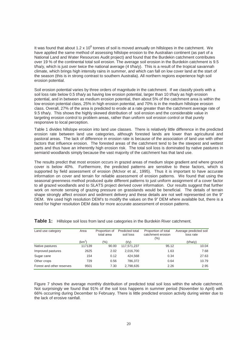
It was found that about 1.2 x 108 tonnes of soil is moved annually on hillslopes in the catchment. Wehave applied the same method of assessing hillslope erosion to the Australian continent (as part of aNational Land and Water Resources Audit project) and found that the Burdekin catchment contributesover 19 % of the continental total soil erosion. The average soil erosion in the Burdekin catchment is 9.5t/ha/y, which is just over twice the national average (4 t/ha/y). This is a result of the tropical savannahclimate, which brings high intensity rains in summer, and which can fall on low cover land at the start ofthe season (this is in strong contrast to southern Australia). All northern regions experience high soilerosion potential.

Soil erosion potential varies by three orders of magnitude in the catchment. If we classify pixels with asoil loss rate below 0.5 t/ha/y as having low erosion potential, larger than 10 t/ha/y as high erosionpotential, and in between as medium erosion potential, then about 5% of the catchment area is within thelow erosion potential class, 25% in high erosion potential, and 70% is in the medium hillslope erosionclass. Overall, 27% of the area is predicted to erode at a rate greater than the catchment average rate of9.5 t/ha/y. This shows the highly skewed distribution of soil erosion and the considerable value intargeting erosion control to problem areas, rather than uniform soil erosion control or that purelyresponsive to local perception.

Table 1 divides hillslope erosion into land use classes. There is relatively little difference in the predictederosion rate between land use categories, although forested lands are lower than agricultural andpastoral areas. The lack of difference in erosion rate is because of the association of land use with otherfactors that influence erosion. The forested areas of the catchment tend to be the steepest and wettestparts and thus have an inherently high erosion risk. The total soil loss is dominated by native pastures insemiarid woodlands simply because the vast majority of the catchment has that land use.

The results predict that most erosion occurs in grazed areas of medium slope gradient and where groundcover is below 40%. Furthermore, the predicted patterns are sensitive to these factors, which issupported by field assessment of erosion (McIvor et al., 1995). Thus it is important to have accurateinformation on cover and terrain for reliable assessment of erosion patterns. We found that using theseasonal greenness method produced quite different patterns to just uniform assignment of a cover factorto all grazed woodlands and to SLATS project derived cover information. Our results suggest that furtherwork on remote sensing of grazing pressure on grasslands would be beneficial. The details of terrainshape strongly affect erosion and sediment delivery and these details are not well represented on the 9"DEM. We used high resolution DEM’s to modify the values on the 9” DEM where available but, there is aneed for higher resolution DEM data for more accurate assessment of erosion patterns.

Table 1: Hillslope soil loss from land use categories in the Burdekin River catchment.

Land use category Area

(km2)

Proportion oftotal area

(%)

Predicted totalsoil loss

(t/y)

Proportion of totalcatchment erosion

(%)

Average predicted soilloss rate

(t/ha/y)Native pastures 117139 90.00 117,571,237 95.12 10.04

Improved pastures 2625 2.02 2,016,700 1.63 7.68

Sugar cane 154 0.12 424,568 0.34 27.63

Other crops 729 0.56 786,372 0.64 10.79

Forest and other reserves 9501 7.30 2,798,635 2.26 2.95

Figure 7 shows the average monthly distribution of predicted total soil loss within the whole catchment.Not surprisingly we found that 91% of the soil loss happens in summer period (November to April) with66% occurring during December to February. There is little predicted erosion activity during winter due tothe lack of erosive rainfall.

21

0

1,000,000

2,000,000

3,000,000

4,000,000

5,000,000

6,000,000

7,000,000

jan feb

mar

chap

rilm

ayjun

ejul

yau

gse

p oct

nov

dec

Months

Pre

dict

edto

tal

soil

loss

(t/y

)

Figure 7: Monthly distribution of predicted total soil loss within the Burdekin River catchment

The contribution of each of the RUSLE factors to the overall pattern of erosion is shown in Figure 8. Thestrong influence of hillslope gradient and rainfall erosivity is shown by these maps, with much of the higherosion hazard occurring on sloping land with high rainfall erosivity. The northern part of the catchmenthas higher rainfall erosivity because of high annual rainfall but also because of greater penetration ofintense summer storms from the coast. The cover factor is usually one of the strongest controls onerosion pattern but in the Burdekin catchment there is relatively little variation because of the relativelyuniform land use across the catchment. Cover in particular years will have strong variation across thecatchment as a result of strong variations in rainfall for that year across the catchment, but over timethese tend to even out to similar mean cover values. Expected differences in cover as a result ofdifferences in inherent soil fertility are not born out by the results and are worthy of further investigation.The precise pattern of erosion hazard within the areas of high slope and rainfall erosivity is influenced bysoil erodibility which varies strongly within individual sub-catchments.

Much of the pattern of surface wash erosion across the catchment could result from natural variation inthe susceptibility to erosion, particularly as the pattern is dominated by slope and rainfall erosivity whichare inherent features of the landscape. Figure 9 compares the natural surface wash erosion potential tothe current potential by incorporating natural vegetation cover, determined from reserve areas in thecatchment. This shows that the overall pattern of erosion predicted for today is broadly similar to thatunder natural conditions. The vast majority of the catchment has a current erosion rate <5 times higherthan the natural rate. There are, however, areas of greatly accelerated erosion hazard in the UpperBurdekin River and Bowen River sub-catchments. In the Upper Burdekin River, these are areas with lowabsolutes rates of erosion so the increase poses little problem but in the Bowen River sub-catchment theyare areas where clearing has increased erosion in areas of high inherent hazard.

Gully Erosion Hazard

It was found that the most robust predictors for discriminating gully density within the Burdekin catchmentwere: landuse, geology, soil texture, rainfall, indices of seasonal climate extremes and terrain-basedattributes such as slope and hill slope length.

22Figure 8: Maps of RUSLE factors that contribute to Figure 6.

23

Figure 9: Pre-European hillslope erosion rate as predicted by the RUSLE, and ratio of current toPre-European results.

24

Among these predictors, elevation, geology, and mean annual rainfall were found to be the mostimportant, producing a correlation coefficient of 0.86 and a relative error of 0.30. The figures wereimproved to 0.96 and 0.14, respectively, when the four MSS bands and relief were added to the model.Further improvements are mainly due to soil attributes. The best overall regression figures are given inTable 2.

Table 2: Best achieved statistical figures of gully density model generated by CUBIST software usingselected climatic and environmental predicting attributes.

Training Set Testing Set

Average error (km km-2) 0.1992 0.3727

Relative Error 0.64 1.15

Correlation coefficient (r) 0.81 0.43

Figure 10 predicts that the majority of gullies form in the central part of the catchment in the areas withmoderately steep slopes on granitic lithologies and on some of the metamorphosed sedimentary rocks.The worst areas are between the Suttor River and Bowen River and in the upper catchments of theClarke and Cape Rivers. Much of the north western and southern parts of the catchment are relativelyunaffected by gully erosion. Very little gully erosion is found on the young mafic volcanics (basalts) as aresult of their stable permeable soils and generally low relief. Similarly the unconsolidated sedimentarymaterials have little erosion because of low gradients and permeable soils. The difference in mappedgully density between geological classes is shown in Figure 11. In addition, the gully mapping done fromaerial photographs revealed that cleared land had much higher gully densities than uncleared land. Themean gully density on cleared land is around 0.68 km/km2, but in areas where the savannah woodlandhas been left uncleared it is around 0.19km/km2. There was good visibility on the aerial photographs forboth land cover cases, so we do not believe this result is due to a measurement bias toward cleared land.The possibility of systematic differences in geology, slope and other factors between cleared anduncleared land were not investigated.

The range of gully densities in the Burdekin river catchment are similar to that found in the moreintensively studied areas of SE Australia. Using that broader context we define a gully density lower than0.1 km/km2 as areas of low gully erosion severity, 0.1 to 1 km/km2 as medium severity, and greater than1 km/km2 as high severity. We found that 2.5% of the catchment (326,000 km2) has high gully erosion,about 70 % faces medium gully erosion and the remaining 27.5 % has no or low gully erosion. Thus,even more so than for hillslope erosion, the problems of gully erosion are highly localised and landmanagement that targets these areas would be more successful than uniform management across thecatchment.

Reconnaissance level analysis of sequential aerial photographs in an area of granodiorite (part of thegranitic complex) suggests that the gullies are still actively eroding headward in contrast to those ofsouthern Australia. We might thus expect annual sediment yields from gullies to be higher than themeasured rates in southern Australia, however there are no such data for northern Australia yet. Thisgap is being filled by work in component R2 of the project. If we assume a typical sediment yield of 50tonnes per kilometre of gully per year then a gully density of 1 km/km2 would result in an areal basedsediment yield of 0.5 t/ha/y, of the same order or lower than might be expected from the hillslopes,although much of the hillslope material may not be delivered to the stream. In gullied landscapes ofhumid areas, the yield from gullies far outweighs the hillslope sediment yield because of denser groundcover and denser gully networks. In those areas sediment control is now focussing largely on gullyerosion control. Our data for the Burdekin catchment suggest a more balanced approach, targetting bothprocesses, is needed for the northern beef industry.

25

Figure 10: Predicted density of gully erosion based on 1.25 km pixels.

26

0

0.1

0.2

0.3

0.4

0.5

0.6

0.7

gran

ites >65

sedim

entar

y 0-65

sedim

enta

ry65

-285

sedim

entar

y >285

felsic

volca

nics >65

felsi

c tom

afic

volca

nics >6

5

maf

icvo

lcanic

s 0-65

Gul

lyde

nsity

(km

/km

2 )

Figure 11: Mean gully density classified by major geology class (lithology and age in My). Granites>65 include granodiorites.

A typical gully would have an eroded depth of 2 m and a width of 5 m giving a total sediment yield of10,000 m3 per kilometre of channel. In the granite/granodirorite areas this would have resulted in a totalsediment yield of approximately 80 t/ha using a sediment density of 1.5 g/cm3 and a gully density of 0.57km/km2. This is the total volume of sediment that is carried by the river network.

Streambank Erosion

Rivers also carry sediment generated from erosion of the river and stream banks themselves, and thisneeds to be considered before examining river sediment loads. One of the two main factors controllingriverbank erosion in the model is the extent of native riparian vegetation, shown in Figure 12. This is onlya crude measure of riparian vegetation because of the 100 m resolution of the vegetation cover dataused. This is, however, the best available data at present. The alternative is to not include bank erosionas a sediment source. This was rejected because reconnaissance level observations suggest that it is anon-trivial contribution to the total catchment sediment budget. To remove riparian vegetation from theprediction of bank erosion results in erroneous results because it predicts that the highest rates of erosionare in National Parks and other reserve areas where there are high energy rivers. Studies of historicalriverbank erosion show that these reserves have not experienced major bank erosion, unlike manycleared streams (Rutherfurd, 2000). The potential for erosion in these areas is prevented by the relativelyundisturbed vegetation. Our mapping of riparian vegetation provides only a first-order overview ofcontrols on bank erosion rate. Higher resolution mapping is required to show the detail within the moreheavily used parts of the catchment.

Figure 12 shows coherent patterns in the proportion of each river link that contains intact native riparianvegetation. The Belyando and Cape Rivers and many of the tributaries of the Burdekin River above theBurdekin Falls Dam have a high proportion of native vegetation cover. Areas of low cover include theBurdekin River below Burdekin Falls Dam, the lower Bowen River, the Suttor River and Diamond andLogan Creek sub catchments.

River discharge is the other factor controlling bank erosion rate in the model. When combined withriparian vegetation the results predict that much of the bank erosion occurs in the lower Burdekin Riverand the lower reaches of the Bowen River where high discharge is combined with a low proportion ofnative riparian vegetation. This matches casual observation where bank erosion of up to 100 m inhistorical times has been reported. The Burdekin River above the Burdekin falls Dam is also predicted to

27

be an area of significant bank erosion, but the potential is not realised in some places because ofsignificant rock outcrop in narrow gorge sections of the river.

Sediment Sources to the Stream Network

Each of the sediment sources described deliver sediment to the network of streams and rivers in theBurdekin River basin. The delivery of sediment to streams from surface wash erosion on hillslopes ismodified by the hillslope sediment delivery ratio. There are very few data from which to define thehillslope sediment delivery ratio. Edwards (1993) observed that hillslope plot erosion measurementsgenerally record about ten times the soil loss as from mini-catchment studies, suggesting a hillslopesediment delivery ratio of around 0.1. In the absence of better information we calibrated the hillslopesediment delivery ratio to produce sediment yields observed near the mouth of the Burdekin Basin. Thisprocess is described below. We found the best results were obtained using a hillslope sediment deliveryratio of 10 %. It was assumed, within the errors of the broad catchment sediment budget, that allsediment derived from gully erosion was delivered to the stream network. Streambank erosion, bydefinition, delivers sediment to the stream network.

Table 3 shows the predicted mean annual amount of sediment supplied to streams from the threeprocesses. Surface wash erosion is the dominant process because of the often low cover and tropicalrainfall in the catchment. Gully and riverbank erosion are also significant sources of sediment. Figure 13shows the spatial pattern of hillslope sediment sources compared to the sum of gully and stream banksources for each sub-catchment. Strong patterns emerge in this map. While hillslope sediment sourcesdominate overall, this is restricted to the near coastal areas where there is the greatest potential forsurface wash erosion. Much of the catchment is predicted to have only a weak dominance of surfacewash erosion, possibly not significant given the uncertainties in the model, or is dominated by gully andstreambank erosion because of the low rates of hillslope erosion. This suggests that all erosionprocesses need to be managed to reduce sediment loads in the catchment. It should be noted thatsurface wash erosion is believed to only contribute to suspended sediment loads, while gully andriverbank erosion contribute relatively equally to bedload and suspended load. When this is taken intoaccount surface wash erosion is the most significant contributor to suspended loads in the basin.

Table 3: Components of the sediment budget for the Burdekin River Basin.

Sediment budget item Predicted meanannual rate

Hillslope delivery 12.3 Mt/y

Gully erosion rate 5 Mt/y

Riverbank erosion rate 1.1 Mt/y

Total sediment supply 18.4 Mt/y

Total suspended sediment stored 13 Mt/y

Total bed sediment stored 3 Mt/y

Sediment delivery from rivers toestuaries 2.4 Mt/y

Total losses 18.4 Mt/y

28

Figure 12: Mapped amount of intact riparian vegetation.

29

Figure 13: Predicted ratio of surface (hill) to subsurface (gully and bank) erosion.

30

Sediment Delivery Through the River Network

On-site erosion hazard is of concern for continued productivity of the land but can only be translated todownstream impacts if the eroded sediment is transported along the river network. The modelledsediment budget for the basin predicts that, overall, only 13 % of sediment delivered to streams isexported at the coast. The rest is stored in floodplains or on the bed of streams, with some storage in thebasin also occurring in reservoirs.

To illustrate the degree of variability of sediment transport within a large basin we first examine some ofthe input data into the predictions before describing the results. This also serves to illustrate the extent ofdata synthesis that has gone into the analysis.

Analysis of the discharge data for the Burdekin river basin showed a good relationship between thedischarge term of sediment transport capacity (ΣQ1.4) and catchment area for each of the gaugingstations but only if the western and southern areas of low relief and low rainfall were treated separatelyfrom the NE part of the catchment. The relationships are shown in Figure 14. The NE part of thecatchment produces seven times the ΣQ1.4 term for a catchment area of 1000 km2 compared to the SWpart of the catchment. Thus, the NE part will have the greater sediment transport capacity for bedload, allother factors being equal. We examined whether the higher discharge per unit area in the NE was afunction of higher rainfall. A regression for the whole basin that also includes mean annual rainfall largelyexplains the difference in behaviour between the two areas. The final method used to predict flow,combined data for the Burdekin river basin with those available for other regions to produce a morecomprehensive model, still based on rainfall and catchment area.

River width increases downstream as the greater discharge carves a wider channel. The rate of increaseinfluences the sediment transport capacity of each reach, as wider channels have slightly lower sedimenttransport capacity. Air photograph analysis showed considerable scatter in width (w in metres) betweenmeasured reaches, but a significant relationship with catchment area (Ax in km2) emerged (Figure 15). Abetter model was produced by including floodplain width (Fx, m) and river slope (Sx) into a multipleregression (r2 = 0.55):

29.05.034.0092.0 xxxx SFAw = . (5)

There is still considerable uncertainty in this relationship but the sediment budget results are relativelyinsensitive to river width so this uncertainty has little effect on the predictions. The effect of river width isoverwhelmed by that of discharge and river slope as outlined below.

The discharge and river width predictions, together with measured river slope, are combined to determinethe sediment transport capacity of each river link. This is the prime control on whether bedload is likely toaccumulate as a result of increased supply of sand and gravel.

Predicted patterns of sediment transport capacity within the basin are shown in Figure 16. These show athree order of magnitude variation from one part of the basin to another. There are very high sedimenttransport capacities in the Burdekin and Bowen Rivers and some of their tributaries. Low sedimenttransport capacities are predicted in the Suttor and Belyando Rivers, considering their catchment area, asa result of both low slope and low discharge. Slope can vary by an order of magnitude from one reach toanother.

31

NE: Q1.4 = 10000A0.90

R2 = 0.907

SW: Q1.4 = 750A0.99

R2 = 0.96

10,000

100,000

1,000,000

10,000,000

100,000,000

1,000,000,000

10 100 1,000 10,000 100,000

Catchment area (km2)

Mea

nan

nual

sum

med

Q1.

4(M

ly-1

)

Figure 14: Regionalisation of the discharge term of streampower (ΣQ1.4) with catchment area for theNE and SW parts of the Burdekin catchment.

w = 5A0.33

10

100

1000

1 10 100 1,000 10,000 100,000 1,000,000

Catchment area (km2)

Cha

nnel

wid

th(m

)

Figure 15: Relationship of river channel width with catchment area for 120 measurements ofchannel cross section from aerial photographs of the Burdekin River catchment.

32

Bedload Deposition

The bedload sediment budget predicts the accumulation of sand and gravel on the bed of rivers as aresult of increased rates of gully and bank erosion. We consider that where historical bed deposition is inexcess of 30 cm, there is likely to be some impact on bed habitats. This might be through filling of pools,smothering of cobble beds with finer grained sediment or reduced diversity of bed forms. Our resultssuggest that only 11 % of the river network length in the basin has bed deposition in excess of 30 cm.This is slightly higher than the national median value of 7 % found by applying the same techniques aspart of the National Land and Water Resources Audit (NLWRA, 2001). The incidence is less though thanmuch of south eastern and south western Australia. The most significant area impacted is that to the eastof the Burdekin Falls Dam, which includes part of the Bowen River catchment (Figure 17). This is an areaof predicted high bedload supply from gully and bank erosion processes and only moderate sedimenttransport capacity. Most areas of the catchment have either a low supply of bedload (the Suttor andBelyando Rivers) or high sediment transport capacity due to the seasonally high discharge (BurdekinRiver and its tributaries). Many rivers in the basin have natural stream beds of sand. This is a commonfeature of semi-arid streams and our results confirm that this is not a feature of river degradation, asmight be suggested from studies of coastal streams in southern Australia.

River Suspended Loads

The river budget for suspended load predicts mean annual suspended loads through the river networkallowing for deposition on floodplains and in reservoirs. Floodplain extent is expected to grow as onetravels downstream and the river becomes larger, and as elevation becomes lower. This pattern can beseen in Figure 18, but there are significant variations which influence the effectiveness of sedimentdelivery. The Cape, Suttor and Belyando Rivers have more extensive lowland floodplains than theBurdekin River and its tributaries or the Bowen River Thus we can expect that there is more efficientsediment delivery through the Burdekin and Bowen Rivers than the others.

The resultant mean annual sediment loads for each river link are shown in Figure 19. The predictedmean annual export to the sea is 2.4 Mt/y. This value is broadly comparable to the results of suspendedsediment monitoring in the lower reaches of the Burdekin River where a mean annual load of 2.8 Mt/y isrecorded (Furnas pers. comm.). Earlier measurements by Belperio (1979) reported a mean annual loadof 3 Mt/y. Sediment loads in tropical rivers are highly variable from one year to another so variationbetween monitoring periods and predicted averages are to be expected.

Our predictions of the natural export to the sea, based on removing gully and bank erosion and using thepre-European rate of hillslope erosion, suggest that the current export is approximately 6 times thenatural rate. This is probably a maximum increase given the harsh assumptions about no gully orriverbank erosion. Unfortunately it is impossible to assess pre-European rates of these processes.

It is the Burdekin and Bowen Rivers that are predicted to contribute much of the suspended sedimentload (Figure 19). The Suttor, Belyando and Clarke Rivers have much lower loads because of both lowersediment supply and extensive lowland floodplains. The other clear feature in Figure 19 is the sharpdecrease in load below the Burdekin falls Dam. The Brune Rule (Brune, 1953) used in the model predictsthat the dam traps 90 % of sediment supplied to it. This is typical for large dams. At such a rate ofdeposition the dam is predicted to be losing 0.1 % of capacity per year. The high trapping efficiency isnot necessarily in conflict with the constant turbidity of the reservoir waters for turbidity can be maintainedby suspension of a low concentration of very fine particles. The bulk of the deposition in the reservoir willbe of the coarser clays, silts and sands. Nevertheless the strongly seasonal flow regime may result in anoverestimation of deposition in the reservoir, as it is calculated using mean annual inflow. A series ofhigh flows in summer, carrying substantial loads will reduce the trap efficiency. The actual amount ofsediment stored in the reservoir can be measured to check the results.

33

Figure 16: Predicted sediment transport capacity.

34

Figure 17: Predicted bedload deposition.

35

Figure 18: Predicted floodplain width.

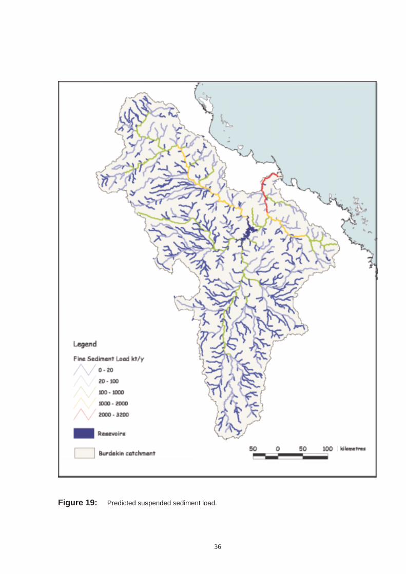
36

Figure 19: Predicted suspended sediment load.

37

Contribution to Sediment Export at the Coast

Estuaries and coastal waters are of particular concern for suspended sediment as they are the ultimateareas of sediment deposition. Along the tropical coast of Queensland estuaries have strong tidal currentsand open mouths. They flush most sediment out to the coastal waters. There, increased rates ofdeposition can smother significant habitats such as sea grass beds and inshore reef communities. Thesediment can also be a supply of nutrient, and change the food web structure. Resuspension of sedimentby waves and currents increases the turbidity of water and decreases light penetration, which can inhibitgrowth of organisms.

Given that only 13 % of sediment delivered to streams within the Burdekin River basin is actuallyexported from the mouth, it cannot be concluded that increased erosion upstream in a sub-catchmentresults in a significant increase to export at the coast. For erosion upstream to link to the coast theremust be efficient delivery of the sediment through the river network. In many of the bigger catchmentsthere are source areas of sediment hundreds of kilometres from the coast and many opportunities for thesediment to be deposited in floodplains or reservoirs as it travels through the river network, as discussedabove.

To further examine sediment export at the coast we have taken the results of our link by link sedimentbudget and worked back up the river network to trace where the sediment comes from. Each river linkcarries sediment contributed from its internal sub-catchment and from tributaries to the link. Each riverlink also deposits a proportion of the mean annual load that it carries. We have worked back up eachtributary to find the contribution from each internal sub-catchment to export from the Burdekin River basin.The result is expressed as a mean annual sediment contribution in t/ha/y from each sub catchment thatreaches the coast.

Sub-catchments which make a substantial contribution to the export at the coast are those with higherosion and limited floodplain extent between the source and sea. Sub-catchments close to the coast aremore likely to contribute to the coastal export because of limited possibilities for that sediment to bedeposited along the way. This is the overall pattern shown by the results (Figure 20). Inland sub-catchments will contribute significant amounts of sediment to the coast if the erosion rate is high and theriver delivers sediment efficiently. Parts of the Burdekin River meet these conditions. The Burdekin FallsDam, however, plays a significant role in reducing sediment delivery from upstream sub-catchments.Much of the Suttor and Belyando catchments export little sediment to the coast, while the Bowen Riversub-catchment is predicted to be a strong contributor.

A result of the very different erosion rates and sediment delivery efficiency is that 95% of sedimentexported to the coast is predicted to come from only 13% of the assessment area. This is in partattributable to the trapping efficiency of the Burdekin Falls Dam, which was dealt with in the section onsuspended sediment loads (p31). While soil erosion is a widespread issue across the Burdekin Riverbasin, targetted management can be used to address specific problems. If the goal is to reduce sedimentloads to the coast then remedial works can be focussed on particular sediment sources and the land usesand erosion processes found there. We predict 85 % of sediment is delivered to the coast from grazinglands in the Bowen River Basin and lower Burdekin. While cane lands only produce 0.8 % of the soilerosion, they are close to the coast and are in sub-catchments which deliver 9 % of the total export at thecoast. These results are produced from a reconnaissance survey and further local investigations areneeded before investing considerable funds in sediment control. The results do, however, provideguidance on where to start those investigations, and they provide testable hypotheses on the sources ofsediment. Sediment delivery to the coast is not the only concern and the same principles can be applied ifthe target is to reduce sediment delivery to particular reservoirs, lakes or individual river reaches of highvalue.

38

Figure 20: Predicted contribution of suspended sediment to the coast for sub-catchments within theBurdekin River catchment.

39

Summary Plots and Calibration of Suspended Sediment Load

The sections above have concentrated on predictions of the river sediment budgets and their implicationswith little discussion on tests of their accuracy. Figure 21 shows a plot of how suspended loads grow withcatchment area from our results. Each point on the plot is the predicted value for a particular river link.This is a common way of summarizing catchment sediment yield data (Walling, 1983). For comparison,measured sediment yields across Australia are plotted on the same basis in Figure 22, as assembled byWasson (1994). There are 278 observations in Figure 22, but only two of them with a catchment area > 1km2 are from central or north Queensland. More data have become available since 1994 but there is astill a paucity of measurement of sediment load patterns. Both graphs show a line fitted by linearregression on a logarithmic plot. The exponent on area in the equation for the line is less than one inboth cases. This means that as catchment area increases there is a less than equal increase in sedimentyield. Small catchments are directly nested within larger catchments, so the yield might be expected togrow equally with catchment area. That it does not, is usually taken as a measure of the intensity ofdeposition along the river length. The coefficient before area in the equation is the sediment yield at acatchment area of 1 km2.

There is considerable scatter of suspended sediment yields about the line in Figure 21. This is to beexpected because of the diverse environments and land use intensity of each sub-catchment. Pointsalong the top of the graph are from the Burdekin and Bowen Rivers. Those along the bottom are from theBelyando and Suttor Rivers. There is a sharp decrease in predicted sediment yield below the BurdekinFalls Dam. This recovers as sediment is supplied from catchments downstream.

There are two poorly defined variables in the suspended sediment model that directly influence theequation of the line in Figure 21. The coefficient in the equation is determined by the average sedimentsupply to streams in the network. This is determined by the rate of bank, gully and hillslope erosion butalso by the value used for hillslope sediment delivery ratio. The hillslope sediment delivery ratio is poorlydefined by measurements in the Burdekin basin or anywhere else. Doubling the hillslope sedimentdelivery ratio significantly increases the supply of sediment to streams. This relative increase is thenpassed on to all river sediment yields downstream and is reflected in a proportional increase in thecoefficient before A. The slope of the line in Figure 21 is determined by the value chosen for the settlingvelocity of suspended sediment on the floodplain. A faster settling velocity means that more sediment willsettle out of the flow for a given residence time on the floodplain. This increases the rate of deposition,decreases the slope of the regression line, and reduces the sediment export from the basin.

We found the best results were produced by using a hillslope sediment delivery ratio of 10% and asediment settling velocity of 1 x 10-6 m/s, equivalent to a silt sized particle. It is possible to set a high avalue for hillslope sediment delivery ratio and compensate for this by simulating very strong deposition onfloodplains, thereby still producing the correct basin sediment yield. There are two indicators which canbe used to prevent this situation. The first is the ratio of sediment derived from hillslopes to that derivedfrom gully and bank erosion. The fallout radionuclide concentrations of sediment can be used to separatehillslope sediment sources from bank and gully erosion (Wallbrink et al., 1998). They indicate that gullyand bank erosion are at least as significant as hillslope erosion in gullied catchments. Preliminarymeasurements in the Burdekin River basin confirm this observation (Olley, pers. comm.). Increasinghillslope sediment delivery ratio makes hillslope erosion dominate in all landscapes.

The second indicator of reasonable parameterisation is the rate of floodplain deposition. Floodplainsaccumulate slowly, at rates of the order of 1 m per 1000 y, or 1 mm/y on average. Our choice offloodplain settling velocity produces a rate at or below 1 mm/y over 72% of the basin. Only in the BowenRiver catchment did rates get higher. This may be an indicator of overestimation of erosion rates in thisarea, as discussed earlier. A further overall indicator of reasonable patterns in the river sediment budgetsis the ratio of bedload to suspended load. Gully and bank erosion contribute evenly to each budget butby the catchment mouth, bedload makes up only 0.1% of the total load, meeting common observations ofsuspended load dominance on large rivers (Richards, 1982).

40

S = 164A0.80

R2 = 0.781

2

2.5

3

3.5

4

4.5

5

5.5

6

6.5

7

0 1 2 3 4 5 6

log catchment area (km2)

log

sedi

men

tyie

ld(t

/y)

Figure 21: Summary of predicted suspended sediment yield across the Burdekin catchment. Eachpoint is a separate river link.

S = 47A0.86

R2 = 0.84

-6

-4

-2

0

2

4

6

8

10

-2 -1 0 1 2 3 4 5 6 7

log catchment area (km2)

log

sedi

men

tyie

ld(t

/y)

Figure 22: Sediment yield data for Australian catchments compiled by Wasson (1994). Only datafor areas >0.01 km2 are shown.

41

Improvements Required

This is the first study to attempt a comprehensive prediction of sediment sources and patterns ofsediment transport within a large regional catchment. Every effort has been made to make the best useof available information and the methods incorporate the current knowledge of large-scale controls onsediment transport processes. As an initial study though there is much scope for improvement, andfurther investigation is warranted if major expenditure on reducing sediment loads is envisaged. Areas ofweakness in understanding at the moment include:

• data on the rates of riverbank erosion;

• higher resolution mapping of riparian condition;

• more comprehensive mapping and prediction of gully erosion;

• the history of sediment supply, particularly from gully erosion;

• independent data on hillslope sediment delivery ratio;

• data on particle size composition of suspended sediment; and

• assessment of the variability of bankfull discharge from one river link to another, which exerts a strongcontrol on deposition potential.

ConclusionsHillslope erosion hazard is clearly very variable across the catchment, with potential erosion hotspotspredominantly located in the NE of the catchment (Douglas, Star, Keelbottom, Fanning sub-catchments)and the Bowen sub-catchment. Equally, gully erosion varies significantly across the catchment beingworst in the central parts of the catchment surrounding the Burdekin Falls Dam on granitic (mainlygranodiorite) lithologies. The patterns of hillslope and gully erosion differ suggesting that each process isfairly independent and that in each location an assessment needs to be made of the dominant source ofsediment. The Burdekin catchment has areas where each process dominates the other. In terms ofnational significance, the catchment has higher than average predicted rates of hillslope erosion, becauseof the tropical rainfall and seasonally poor cover.

The development of improved grazing management guidelines will need to be specially adapted to theparticular soil-pasture communities prevalent in those sub-catchments or landscapes identified ashotspots. To achieve maximum impact on reduction of sediment loss, they also need to be differentiatedto specifically address hillslope or gully erosion, whichever is the more important form of erosion in aparticular area. The outputs from this research component should therefore assist the grazing industry,extension providers and natural resource management agencies to appropriately target the critical areas,so that a comparatively large benefit in reducing sediment loads delivered downstream can be achievedwith less effort.

Despite the moderate gully erosion and bank erosion few of the streams appear to be impacted byincreased bedload. This is because of the high energy of many of the effected streams. Many areas inAustralia that have had dramatic changes to the morphology of river beds are where there has beencatastrophic widening of the streams themselves or intense gully erosion and the Burdekin Rivercatchment has not experienced this. The Bowen River and area surrounding the Burdekin Falls Dam,however, could be impacted by sediment deposition.

Suspended sediment loads in rivers are on average predicted to have increased by 15 times. Theassumptions used in that analysis were fairly harsh, as that was all that was possible given the data.Even so, there are clearly substantial increases to suspended sediment loads and the possibility ofpredicted in-stream impacts as a result of those changes cannot be dismissed.

42

Sediment export to the coast has increased by as much as 6 times. It si predicted that 95% of thissediment comes from 13% of the land. Potential impacts on sea grass beds, in-shore reefs and othermarine organisms cannot be dismissed. The highly specific source of the sediment provides a clearfocal point for further assessment and targeting the control of sediment delivery to streams.

Finally, another important conclusion from the work to date is that we can derive some relatively simple,yet robust regionalisation rules for the assessment of sediment delivery hazard based on basic attributessuch as rainfall, topography and catchment size. This will greatly facilitate the extrapolation of resultsobtained in the Burdekin to other catchments in Northern Australia, as these attributes are readilyavailable. The accurate measurement of ground cover and its changes over time is critical to futureassessment of soil erosion problems in the semi-arid tropics.

ReferencesBelperio, A. P. (1979). The combined use of wash load and bed material load rating curves for the

calculation of total load: an example from the Burdekin River, Australia. Catena, 6: 317-329.

Bonell, M. and Williams, J. (1987). Infiltration and redistribution of overland flow and sediment on a lowrelief landscape of semi-arid, tropical Queensland. IAHS Publication, No. 167: 199-211.

BRS, (2000). http://www.brs.gov.au:80/land&water/landcov/alcc_results.html

Brune, G.M. (1953). Trap efficiency of reservoirs. Transactions, American Geophysical Union, 34(3): 407-418.

Dietrich, W.E. and Dunne, T. (1978). Sediment budget for a small catchment in mountainous terrain.Zeitschrift fur Geomorphologie, 29:191-206.

Edwards, K. (1993). Soil erosion and conservation in Australia. In Pimental, D. (Ed.), World Soil Erosionand Conservation. Cambridge University Press, Cambridge, 147-69.

Gallant, J. (2001). Topographic scaling for the NLWRA sediment project. Technical Report 27/01, CSIROLand and Water, Canberra.

Heinemann, H.G. (1981). A new sediment trap efficiency curve for small reservoirs. Water ResourcesResearch, 17:825-830.

Hughes, A. O., Prosser, I. P., Stevenson, J., Scott, A., Lu H., Gallant J. and Moran, C.J. (submitted).Gully Density Prediction for the Intensive Landuse Zone of Australia. Technical Report **/01,CSIRO Land and Water, Canberra.

Jeffers, J.N.R. (1998). Characterisation of river habitats: a prediction of habitat features using ordinationtechniques. Aquatic Conservation: Marine and Freshwater Ecosystems, 8: 529-540.

Littleboy, M., Silburn, D.M., Freebairn, D.M., Woodruff, D.R., Hammer, G.L., and Leslie, J.K. (1992).Impact of soil erosion on production in cropping systems. I. Development and validation of asimulation model. Australian Journal of Soil Research, 30(5): 757-774.

Lu, H., Gallant, J., Prosser, I.P., Moran, C., and Priestley, G. (2001). Prediction of Sheet and Rill ErosionOver the Australian Continent, Incorporating Monthly Soil Loss Distribution. Technical Report13/01, CSIRO Land and Water, Canberra.

McCool, D.K., Foster, G.R., Mutchler, C.K., and Meyer, L.D. (1989). Revised slope length factor in theUniversal Soil Loss Equation. Transactions of the American Society of Agricultural Engineers, 32:1571-1576.

43

McIvor, J.G., Williams, J. and Gardener, C.J. (1995). Pasture management influences runoff and soilmovement in the semi-arid tropics. Australian Journal of Experimental Agriculture, 35: 55-65.

McKenzie, N.J., Jacquier, D.W. Ashton, L.J. and Cresswell, H.P. (2000). Estimation of soil propertiesUsing the Atlas of Australian Soils. CSIRO Land and Water, Technical Report 11/00.

Meade, R.H. (1982). Sources, sinks and storage of river sediment in the Atlantic Drainage of the UnitedStates. Journal of Geology, 90:235-252.

Moore, I.D. and Burch, G.J. (1986). Physical basis for the length-slope factor in the universal soil lossequation. Soil Science Society of America Journal, 50: 1294-1298.

Nicholas, A.P., Ashworth, M.J., Kirkby, M.J., Macklin, M.G. and Murray, T. (1995). Sediment slugs: large-scale fluctuations in fluvial sediment transport rates and storage volumes. Progress in PhysicalGeography, 19:500-519.

NLWRA (2001). Ecosystem Health 2000. National Land and Water Resources Audit, Canberra.

Olive, L.J. and Walker, P. H. (1982). Processes in Overland Flow - Erosion and Production of SuspendedMaterial. In E.M. O'Loughlin and P. Cullen (Editors) Prediction in Water Quality. AustralianAcademy of Science, Canberra, 87-119.

Pickup, G. and Marks, A. (2001). Identification of floodplains and estimation of floodplain flow velocitiesfor sediment transport modelling. NLWRA Sediment Project (CLW 12). CSIRO Land and WaterTechnical Report 14/01, Canberra.

Prosser, I.P. and Williams, L. (1998). The impact of wildfire on runoff and erosion in native Eucalyptusforest. Hydrological Processes, 12: 251-265.

Prosser, I.P., Hughes, A.O., Rustomji, P., Young W., and Moran, C.J. (2001). Assessment of RiverSediment Budgets for the National Land and Water Resources Audit. CSIRO Land and WaterTechnical Report 15/01, Canberra.

Quinlan, J. R. (1993). C4.5: Programs for Machine Learning, Morgan Kaufmann Publishers, San Mateo,California.

Renard, K.G., Foster G. A., Weesies D. K., McCool, D.K., and Yoder, D.C. (1997). Predicting soil erosionby water: A guide to conservation planning with the revised universal soil loss equation .Agriculture Handbook 703, United States Department of Agriculture, Washington DC.

Richards, K. (1982). Rivers, Form and Process in Alluvial Channels. Methuen. London.

Rosewell, C.J. (1993). SOILOSS - A program to assist in the selection of management practices toreduce erosion. Technical Handbook No. 11 (2nd edition) Soil Conservation Service of NSW,Sydney.

Rutherfurd, I. (2000). Some human impacts on Australian stream channel morphology. Brizga, S. andFinlayson, B. River Management: The Australasian Experience. Chichester, John Wiley & Sons.

Rutherfurd, I.D. (1996). A Sand Management Strategy for the Glenelg River, South-West Victoria.Report to the Department of Natural Resources, Victoria. Melbourne.

Scanlan, J.C., Pressland A. J. and Myles D. J. (1996). Run-off and soil movement on mid-slopes in north-east Queensland grazed areas. Rangeland Journal, 18: 33-46.

Shreve, R.L. (1966). Statistical law of stream numbers. Journal of Geology, 74:17-37.

44

Trimble, S.W. (1981). Changes in sediment storage in the Coon Creek Basin, Driftless area, Wisconsin.Science, 214:181-183.

Van Dijk, P.M. and Kwaad, F.J.P.M. (1998). Modelling suspended sediment supply to the River Rhinedrainage network: a methodological study. International Association of Hydrological Sciences,Publ. No. 249:165-176.

Wallbrink, P.J., Olley, J. M., Murray, A. S. and Olive L. J. (1998). Determining sediment sources andtransit times of suspended sediment in the Murrumbidgee River, NSW, Australia using fallout137Cs and 210Pb. Water Resources Research, 34:879-887.

Walling, D.E. (1983). The sediment delivery problem. Journal of Hydrology, 65:209-237.

Walling, D.E., Quine, J. A. and He, Q. (1992). Investigating contemporary rates of floodplainsedimentation. In Carling, P. A. and Petts, G. E. (editors) Lowland Floodplain Rivers:Geomorphological Perspectives. Chichester, Wiley, 166-184.

Wasson, R.J., (1994). Annual and decadal variation of sediment yield in Australia, and some globalcomparisons. International Association of Hydrological Sciences Publ., 224: 269-279.

Williams, G.P. (1989). Sediment concentration versus water discharge during single hydrologic events.Journal of Hydrology, 111:89-106.

Williams, J.R. (1977). Sediment delivery models determined with sediment and runoff models. AIHS-AISHpublication, 122:168-179.

Wischmeier, W. H. and Smith, D. D. (1978). Predicting rainfall erosion losses: A guide to conservationplanning. US Department of Agriculture. Agriculture Handbook No. 537. US Government PrintingOffice: Washington, DC.

Yang, C.T. (1973). Incipient motion and sediment transport. Journal of the Hydraulics Division, ASCE.99:1679-1704.

Documents

Regional Patterns of Erosion and Sediment Transport in the Burdekin ... - Land and Water · 2005-10-14 · Regional Patterns of Erosion and Sediment Transport in the Burdekin River