water

Article

Regional Parameter Estimation of the SWAT Model:Methodology and Application to River Basins in thePeruvian Pacific Drainage

Flavio Alexander Asurza-Véliz * and Waldo Sven Lavado-Casimiro

Dirección de Hidrología, Servicio Nacional de Meteorología e Hidrología del Perú (SENAMHI),Lima 15072, Peru; wlavado@senamhi.gob.pe* Correspondence: falexav@gmail.com

Received: 15 September 2020; Accepted: 6 November 2020; Published: 16 November 2020 �����������������

Abstract: This study presents a methodology for the regional parameters estimation of the SWAT(Soil and Water Assessment Tool) model, with the objective of estimating daily flow series in the Pacificdrainage under the context of limited hydrological data availability. This methodology has beendesigned to obtain the model parameters from a limited number of basins (14) to finally regionalizethem to basins without hydrological data based on physical-climatic characteristics. In addition,the bootstrapping method was selected to estimate the uncertainty associated with the parametersset selection in the regionalization process. In general, the regionalized parameters reduce the initialunderestimation which is reflected in a better quantification of daily flows, and improve the lowflows performance. Furthermore, the results show that the SWAT model correctly represents thewater balance and seasonality of the hydrological cycle main components. However, the model doesnot correctly quantify the high flows rates during wet periods. These findings provide supportinginformation for studies of water balance and water management on the Peruvian Pacific drainage.The approach and methods developed can be replicated in any other region of Peru.

Keywords: regional parameters; SWAT; daily flows; Peruvian Pacific drainage

1. Introduction

The basins that drain into the Pacific Ocean of Peru are characterized by small basins with bareand steep slopes that favor erosion and flooding during intense rainfall events. Rainfall is moreabundant along the north coast and decreases towards the south, where conditions are extremelyarid [1]. The Pacific drainage represents 22% of the Peruvian territory [2], where more than 50%of the Peruvian population is established and has 2% of all the fresh water available in Peru [3],generating frequent conflicts between multiple water users regarding its allocation and accessibility.Currently, 73% of the population lives in urban environments, and it is expected that it (as well astheir living standards) will increase by 2050 to approximately 40 million [4]. Therefore, domestic andagricultural water use is likely to increase rapidly, even more so in a country where much of the currentagricultural production depends on irrigation and consumes approximately 85% of surface water [5].Despite the importance of knowing water availability in Peru, previous studies [6–8] have shownevidence of the limited hydrological data availability in the Pacific drainage (Pd).

The evaluation of the water availability of a basin is generally performed through hydrologicalmodels. Rainfall–runoff modeling is an important area of research for the global scientific communitythat addresses the hydrology. A simple reason for this is that quantitative or qualitative flowinformation is vital for many practical applications, such as water allocation, long-term planning,watershed management operations, flood forecasting, optimization of the hydroelectric power

Water 2020, 12, 3198; doi:10.3390/w12113198 www.mdpi.com/journal/water

Water 2020, 12, 3198 2 of 26

production, and the hydraulic structures design. Although hydrological models can provideinformation on the rainfall–runoff mechanism, they remain abstractions of a real system, and itcannot be assumed that any of them generate accurate information for specific hydrographic basinsand hydrological conditions [9]. Hydrological modeling requires calibration, which to a certain extentoffers a reliability of the the measured flow rates simulations, especially in the context of (1) lackof hydrological process understanding, (2) possibly too simplistic representations of the process(abstractions), (3) the spatio-temporal discretization of highly heterogeneous rainfall–runoff processes,and (4) the impossibility of measuring all the model parameters required in the application scale [10].In addition, in regions with little measured hydrological data, such as Peru, the set of parameterstransfer of a calibrated model from one or more basins to a basin without hydrological data is a validtool to quantify the hydrological processes that occur within them. This process of transfer is knownas regionalization [11].

Flow regionalization is a challenging task in the hydrology science [12–14]. First, due to theabsence of flow data required for the model calibration, and second, studies evaluating regionalizationmethods usually produce different results [12]. Despite this research momentum, there is still nosingle accepted approach to predict flows in regions with no hydrological data [15,16]. A largenumber of hydrological models regionalization methods have been proposed in the literature. All ofthem are based on the concept that information on the hydrological response can be transferredbetween hydrographic basins that can be assumed to be hydrologically similar, generally basedon the knowledge of their relevant physical properties. The differences between the approachesare found in the type of information that is transferred, the method used and the watershedproperties used to quantify the similarity. There are at least three common regionalization approaches:the regression-based approach, the spatial proximity approach, and the physical similarity approach.Comparative studies have been conducted in small and large data sets, in multiple hydrologicalmodels and with many variants [12,17–21]. The authors of [16] conducted an exhaustive review ofregionalization studies during the last decade. The most notable studies have had some divergentresults, which are part of the reason why more conclusive evidence is required [12,22]. Most studiesuse simple hydrological models with few parameters to preserve a high level of independence anda good correlation between the parameters and the basins descriptors. For hydrological modelswith small parameter spaces and low parameter interdependence, equifinality is often not a problem.However, if the hydrological model has the opposite attributes, many optimal parameter sets can befound during calibration. The current modeling philosophy requires that the models be describedtransparently and that the uncertainty analysis be performed routinely as part of the modeling work.This analysis is essential to evaluate the calibrated model strength [23,24].

The SWAT (Soil and Water Assessment Tools) model [25] has shown its strengths in theaspects detailed above. It has been used both to quantify uncertainty and evaluate regionalizationmethods [24,26–30]. In addition, the SWAT model is open source with a large and growing numberof applications in hydrological modeling applied in studies ranging from basin scale to continentalscales. There are few published studies related to SWAT in South America for flow estimationpurposes [31–35]. In Peru, its use is not yet widespread [36,37], although hydrological modelsranging from aggregated to semidistributed have been used in recent years. The references showthat the models in Peru have been developed mainly to evaluate the impact of climate change onhydrology [38–41], the evaluation of satellite rainfall products for hydrology purposes [42–46] andthere is only one study that performs a parameters regionalization at the scale of the Pd using a lumpedhydrological model [8]. During recent years, some hydrological studies have been developed onthe Peruvian Pd: [47] documented and analyzed the previous hydrological and physical conditionsthroughout the study area (54 hydrographic basins) from the 1920 to the 1960s. The authors of [3]evaluated the water supply and demand in the main basins where water management is prioritized.They estimated the total annual volume of fresh water available throughout the Pd from the 1970s to2010. The authors of [6] analyzed mean conditions and flow variability from 1969 to 2004. The authors

Water 2020, 12, 3198 3 of 26

of [48] identified the annual runoff for some hydrographic basins with low water balance disparitiesor with quasi-natural conditions on an interannual scale from 1970 to 2008. Finally, [8] quantifiedand analyzed the flow variability and seasonality in natural regime in 49 Pd basins by applying aparameters regionalization methodology from conceptual models. There have been numerous effortsto evaluate and quantify the water resources in the Pd during recent years; however, there are still noregional studies with the purpose of estimating natural series of daily flows.

In this context, the objective of this work is to use SWAT to build a hydrological model for thePd at subbasin level and at a daily time step. The key objectives of this work are (1) to present for thefirst time a regionalization parameters methodology based on a physical basis model, (2) to estimatewater availability in the period 1981–2016 under a context of data scarcity, and (3) to quantify theuncertainty associated with the parameter regionalization process. In particular, components suchas blue water (water yield plus deep aquifer recharge), green water flow (real evapotranspiration)and green water storage (soil moisture) are quantified. The estimates of the model at subbasin levelare added to basin levels to compare it with previous studies and to support the obtained results.This article is organized as follows: Section 3 briefly describes the structure of the SWAT model andexplains the proposed methodology. The calibration results, the estimated regional flow statisticalperformance and the uncertainty analysis are discussed in Sections 4 and 5. Finally, Section 6 providesthe summary and conclusions of this study.

2. Study Area

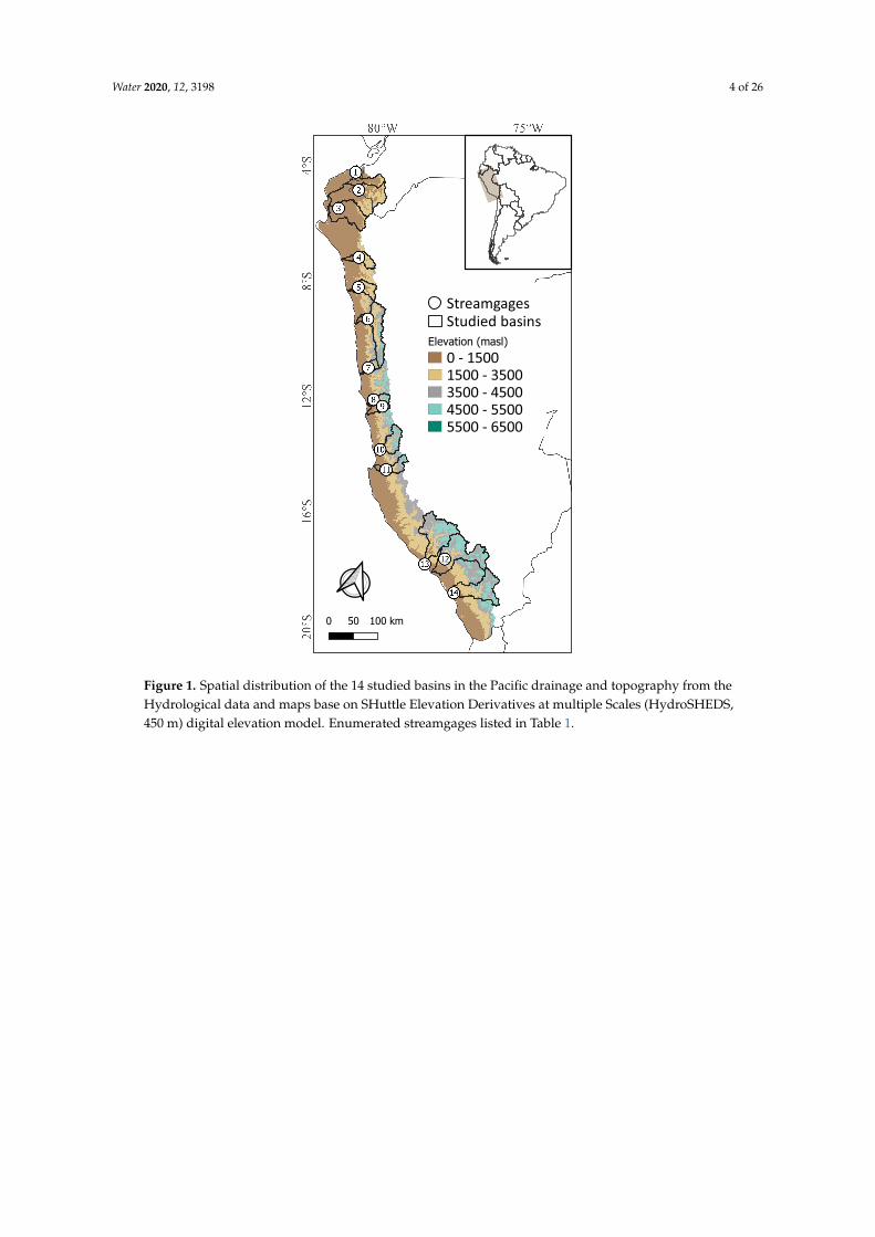
The Pacific drainage (Pd) has an approximate area of 278,482 km2. The study region includes52 main hydrographic basins with altitudinal variations ranging from 0 to approximately 6500 masl(Figure 1). These basins have bare and steep slopes and generally drain west from the high Andes tothe Pacific Ocean. In addition, during heavy rainfall events, a high potential for increased maximumflows, floods and erosion prevails in the Pd [6,48].

Under normal conditions, this region is influenced by the South Pacific Anticyclone in combinationwith the Humboldt Current, which produces dry and stable conditions in the western central Andes.Additionally, this region exhibits greater seasonal and interannual rainfall variability than the othertwo main hydrological regions of Peru: the Titicaca and Amazon drainages [6], mainly caused by theinfluence of the El Niño Southern Oscillation (ENSO). ENSO generates impacts on the regional climateworldwide, particularly on the Pacific coast, and these impacts are reflected in the strong El Niño years,which has a direct influence on rainfall increase (decrease) in the northern (southern) zone [7,49–51],also causing large economic losses [52].

The study area presents arid and semiarid conditions and, therefore, is prone to threats of waterscarcity for different sectors. The water demand for economical activities (agriculture, mining, industryand livestock) and domestic use represent approximately 87% of the total national consumption.Only agriculture represents the greatest consumptive use (86%), whose availability depends mainly onthe irrigation systems located in the basins valleys. In addition to the threat of water scarcity, Pd isprone to devastating floods [3].

Water 2020, 12, 3198 4 of 26

StreamgagesStudied basins

Elevation (masl)

0 - 15001500 - 35003500 - 45004500 - 55005500 - 6500

Figure 1. Spatial distribution of the 14 studied basins in the Pacific drainage and topography from theHydrological data and maps base on SHuttle Elevation Derivatives at multiple Scales (HydroSHEDS,450 m) digital elevation model. Enumerated streamgages listed in Table 1.

Water 2020, 12, 3198 5 of 26

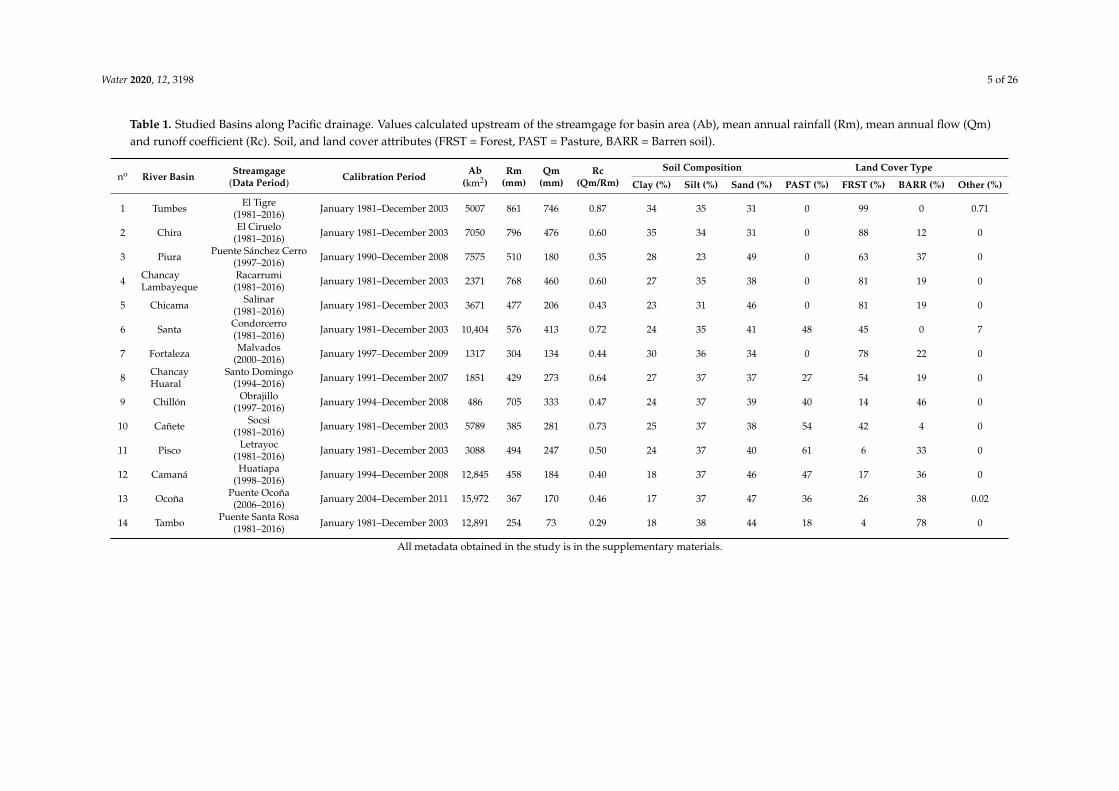
Table 1. Studied Basins along Pacific drainage. Values calculated upstream of the streamgage for basin area (Ab), mean annual rainfall (Rm), mean annual flow (Qm)and runoff coefficient (Rc). Soil, and land cover attributes (FRST = Forest, PAST = Pasture, BARR = Barren soil).

no River Basin Streamgage(Data Period) Calibration Period

Ab(km2)

Rm(mm)

Qm(mm)

Rc(Qm/Rm)

Soil Composition Land Cover Type

Clay (%) Silt (%) Sand (%) PAST (%) FRST (%) BARR (%) Other (%)

1 TumbesEl Tigre

(1981–2016) January 1981–December 2003 5007 861 746 0.87 34 35 31 0 99 0 0.71

2 ChiraEl Ciruelo

(1981–2016) January 1981–December 2003 7050 796 476 0.60 35 34 31 0 88 12 0

3 PiuraPuente Sánchez Cerro

(1997–2016) January 1990–December 2008 7575 510 180 0.35 28 23 49 0 63 37 0

4ChancayLambayeque

Racarrumi(1981–2016) January 1981–December 2003 2371 768 460 0.60 27 35 38 0 81 19 0

5 ChicamaSalinar

(1981–2016) January 1981–December 2003 3671 477 206 0.43 23 31 46 0 81 19 0

6 SantaCondorcerro(1981–2016) January 1981–December 2003 10,404 576 413 0.72 24 35 41 48 45 0 7

7 FortalezaMalvados

(2000–2016) January 1997–December 2009 1317 304 134 0.44 30 36 34 0 78 22 0

8ChancayHuaral

Santo Domingo(1994–2016) January 1991–December 2007 1851 429 273 0.64 27 37 37 27 54 19 0

9 ChillónObrajillo

(1997–2016) January 1994–December 2008 486 705 333 0.47 24 37 39 40 14 46 0

10 CañeteSocsi

(1981–2016) January 1981–December 2003 5789 385 281 0.73 25 37 38 54 42 4 0

11 PiscoLetrayoc

(1981–2016) January 1981–December 2003 3088 494 247 0.50 24 37 40 61 6 33 0

12 CamanáHuatiapa

(1998–2016) January 1994–December 2008 12,845 458 184 0.40 18 37 46 47 17 36 0

13 OcoñaPuente Ocoña

(2006–2016) January 2004–December 2011 15,972 367 170 0.46 17 37 47 36 26 38 0.02

14 TamboPuente Santa Rosa

(1981–2016) January 1981–December 2003 12,891 254 73 0.29 18 38 44 18 4 78 0

All metadata obtained in the study is in the supplementary materials.

Water 2020, 12, 3198 6 of 26

3. Materials and Methods

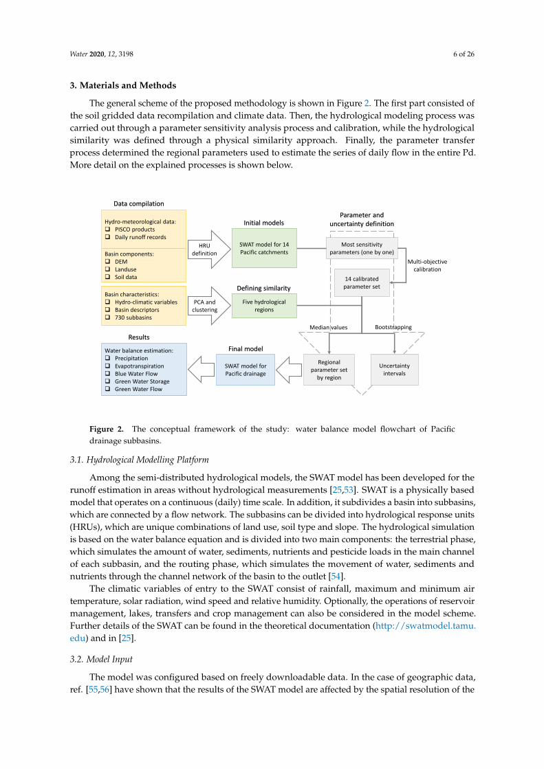
The general scheme of the proposed methodology is shown in Figure 2. The first part consisted ofthe soil gridded data recompilation and climate data. Then, the hydrological modeling process wascarried out through a parameter sensitivity analysis process and calibration, while the hydrologicalsimilarity was defined through a physical similarity approach. Finally, the parameter transferprocess determined the regional parameters used to estimate the series of daily flow in the entire Pd.More detail on the explained processes is shown below.

Hydro-meteorological data: PISCO products Daily runoff records

Five hydrologicalregions

Basin characteristics: Hydro-climatic variables Basin descriptors 730 subbasins

Data compilation

SWAT model for 14 Pacific catchments

Defining similarity

14 calibratedparameter set

Regional parameter set

by region

Bootstrapping

Most sensitivityparameters (one by one)

Median values

Results

SWAT model for Pacific drainage

Water balance estimation: Precipitation Evapotranspiration Blue Water Flow Green Water Storage Green Water Flow

Uncertaintyintervals

HRU definition

PCA and clustering

Basin components: DEM Landuse Soil data

Parameter and uncertainty definitionInitial models

Final model

Multi-objectivecalibration

Figure 2. The conceptual framework of the study: water balance model flowchart of Pacificdrainage subbasins.

3.1. Hydrological Modelling Platform

Among the semi-distributed hydrological models, the SWAT model has been developed for therunoff estimation in areas without hydrological measurements [25,53]. SWAT is a physically basedmodel that operates on a continuous (daily) time scale. In addition, it subdivides a basin into subbasins,which are connected by a flow network. The subbasins can be divided into hydrological response units(HRUs), which are unique combinations of land use, soil type and slope. The hydrological simulationis based on the water balance equation and is divided into two main components: the terrestrial phase,which simulates the amount of water, sediments, nutrients and pesticide loads in the main channelof each subbasin, and the routing phase, which simulates the movement of water, sediments andnutrients through the channel network of the basin to the outlet [54].

The climatic variables of entry to the SWAT consist of rainfall, maximum and minimum airtemperature, solar radiation, wind speed and relative humidity. Optionally, the operations of reservoirmanagement, lakes, transfers and crop management can also be considered in the model scheme.Further details of the SWAT can be found in the theoretical documentation (http://swatmodel.tamu.edu) and in [25].

3.2. Model Input

The model was configured based on freely downloadable data. In the case of geographic data,ref. [55,56] have shown that the results of the SWAT model are affected by the spatial resolution of the

Water 2020, 12, 3198 7 of 26

aforementioned data. Therefore, the resolutions considered below were selected based on the dataavailability for the Pd and the size of subbasins to be delimited (as discussed later in this section).

• The rainfall and temperature data were obtained from the product PISCO (Peruvian Interpolateddata of Senamhi’s Climatological and Hydrological Observations). The daily rainfall databasecorresponded to version 2.1 [57], while the daily temperature database (maximum and minimum)was version 1.1 [58]. Both products are available from January 1981 to December 2016 and have aspatial resolution of 0.1 degree (∼10 km). These databases are available on the IRI Climate DataLibrary website (http://iridl.ldeo.columbia.edu/SOURCES/.SENAMHI/.HSR/.PISCO/index.html?Set-Language=es).

• The 450-m digital elevation model (DEM) was obtained from HydroSHEDS (Hydrological dataand maps base on SHuttle Elevation Derivatives at multiple Scales). This product is based onhigh-resolution elevation data obtained from SRTM (Shuttle Radar Topography Mission) [59].

• The 300-m land-use map used corresponds to 2015 and was obtained from the ESA CCI-LC(European Space Agency and Climate Change Initiative-Land Cover) project [60].

• The 8 km soil type map was obtained from FAO-UNESCO. The map for Volume IV SouthAmerica [61] was taken, which gridded data was released in 2006.

Flow data from 14 streamgages were obtained from the National Service of Meteorology andHydrology of Peru (SENAMHI). The observed daily flow series meet the following requirements:(1) have at least 10 years of record in the period 1981–2016, (2) the series are only minimally affected byextractions, transfer, and dams; (3) the flow series corresponds to the main basins and covers much ofthe total area of the Pd.

3.3. Model Setup

The model was implemented in SWAT 2012 using the QSWAT interface [62]. For the subbasinsdelimitation, two criteria were taken: (1) the burn-in option was used from predefined rivers to improvethe delimitation in flat areas [63], and (2) an area threshold was established to be 200 km2. In addition,the HRUs were defined based on land use, soil type and dominant slope. This configuration wasconsidered appropriate according to the computational resources available for hydrological modelingat the drainage scale.

The potential evapotranspiration was estimated by the Hargreaves–Samani method [64] dueto the limited and scarce availability of observed data on relative humidity, wind speed and solarradiation. In addition, this method has shown good results comparable with Priestley–Taylor [65] andPenman–Monteith [66] (methods also available in SWAT) in semiarid zones [67]. The model did notinclude data on reservoirs operation, lakes or any other hydraulic influence.

3.4. Model Calibration

The SWAT input parameters are based on real processes and must be kept within a range ofrealistic uncertainty, so the first step in the calibration process was determinate the most sensitiveparameters of the hydrological model [68]. In this way, from a sensitivity analysis for each parameter(one-at-a-time), the search ranges of each parameter were identified (ranges that respected the physicalmeaning of each one) so that the SWAT model is able to quantify the flow contributed by surface runoffand baseflow. In addition, as recommended by [69], it was considered to calibrate the model with thefewest possible parameters.

3.4.1. Evaluation Metrics

The calibration process considered a warm-up period of 3 years, and the statistical performancewas evaluated based on the Kling–Gupta efficiency criterion (KGE) and the logarithmic Nashindex (logNSE).

Water 2020, 12, 3198 8 of 26

• Overall performance: KGE is a comprehensive metric, a weighted average of the Pearsonproduct-moment correlation coefficient (r), the ratio between the mean of the simulated valuesand the mean of the observed ones (β), and variability ratio (γ), which is computed using thestandard deviation of simulated and observed (Equation (1)). Kling–Gupta efficiencies rangefrom –Infinity to 1. The closer to 1, the more precise the model is.

KGE =√(r− 1)2 + (β− 1)2 + (γ− 1)2 (1)

• Low flows: By taking the log of simulated (log Si) and observed (log Oi) before calculating theNSE, the influence of (missing) peak flows is reduced and more emphasis is placed on the baseflow (the criticism of the standard NSE is that it is overly sensitive to the magnitude and timingof peak flows (Equation (2)).

logNSE = 1− ∑ni=1(log Oi − log Si)

2

∑ni=1(log Oi − log O)2 (2)

Maximizing the KGE and logNSE, the performance of the hydrological modeling was optimizedfrom a multi-objective perspective using the correlation, variability and bias criteria [70] and theperformance in the representation of low flow rates. These statistics have been used in previousstudies, resulting in good calibration and good performance in hydrological modeling [71–73].

The calibration and validation of the simulated and observed flows performance was carried outin 14 basins with daily flow data availability. The calibration period indicated in Table 1 was usedto obtain the calibrated parameters. Then, we validate the performance of the model in two periods:the subsequent period to the calibration period until December 2016 and the entire period 1981–2016.The goodness of fit parameters were estimated through the R package “hydroGOF” [74].

3.4.2. Multiobjective Calibration Algorithm

The optimal parameters were derived from the Elitist Non-dominated Sorting Genetic AlgorithmII (NSGA-II) multi-objective calibration algorithm, whose application has provided excellent results inhydrological modeling using SWAT and has been shown to be more efficient than the Monte Carlomethod to reduce optimized parameters uncertainty [75,76]. Unlike single objective genetic algorithms,NSGA-II assigns fitness by Pareto ranking (nondomination) and crowding distance to the combinedparent and child populations. A solution (or individual) is nondominated if it performs better in at leastone objective functions and as well in all the other objective functions. The individual is then rankedaccording to the number of solutions that dominates it. Crowding distance is the average distancebetween an individual and its nearest neighbors in the search space. With the objective functionsas minimization problems, individuals that are dominated by fewer solutions (i.e., has a lowerrank) are given a better fitness than the dominated ones. In cases where the solutions have the samenondomination rank, the individual with larger crowding distance is preferred, thus ensuring diverseand well-spread population. The new parent population is chosen from the combined parent and childpopulation based on the individuals’ fitness or rank, thus the elitist selection.

NSGA-II nondominated sorting algorithm has a computational complexity O(MN2), where Mis the number of objectives and N is the size of a population P. For each solution two parametersare calculated in the algorithm: (1) the domination count ni which is the number of solutions thatdominate the solution i and (2) a set of solutions Si that the solution i dominates. The solutions of thefirst non-dominated front are identified in Steps 1 to 3 of the algorithm and the solutions in higherfronts are searched in Steps 4 to 6. The algorithm is as follows:

• Step 1: For each i ∈ P, set ni = 0 and Si = Ø.• Step 2: For all j 6= i and j ∈ P, if i dominates j, Add j to the set of solutions dominated by i: Si = Si

U j. Otherwise, increment the domination count of i: ni = ni +1.

Water 2020, 12, 3198 9 of 26

• Step 3: If ni = 0, keep i in the first non-dominated front P1 and set the front counter k = 1.• Step 4: While Pk 6= Ø, initialize Q = Ø for storing the next non-dominated solutions.• Step 5: For each i ∈ Pk and for each j ∈ Si, update nj = nj – 1. If nj = 0, j belongs to the next front

and update Q = Q U j.• Step 6: Set k = k +1 and Pk = Q, go to Step 4.

Further details of NSGA-II can be found in [77]. The calibration algorithm was implementedthrough the R library “nsga2R” [78], setting KGE and logNSE as objective functions.

3.5. Regionalization Using the Physical Similarity Approach

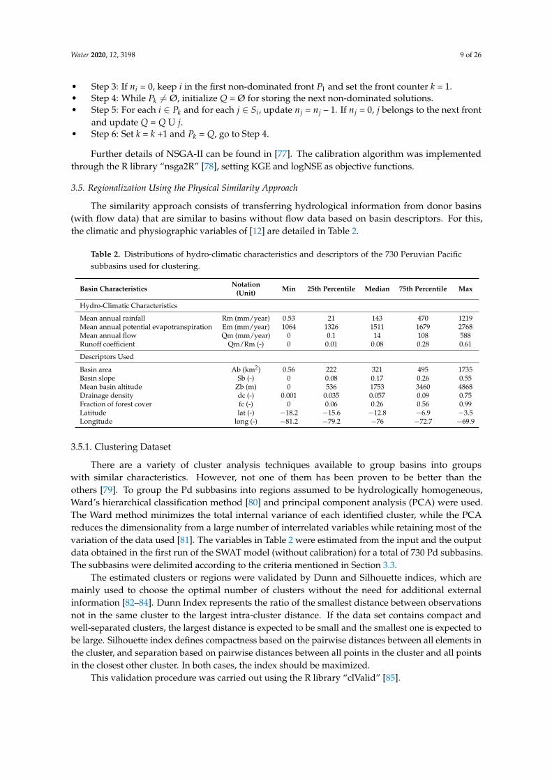
The similarity approach consists of transferring hydrological information from donor basins(with flow data) that are similar to basins without flow data based on basin descriptors. For this,the climatic and physiographic variables of [12] are detailed in Table 2.

Table 2. Distributions of hydro-climatic characteristics and descriptors of the 730 Peruvian Pacificsubbasins used for clustering.

Basin Characteristics Notation(Unit) Min 25th Percentile Median 75th Percentile Max

Hydro-Climatic Characteristics

Mean annual rainfall Rm (mm/year) 0.53 21 143 470 1219Mean annual potential evapotranspiration Em (mm/year) 1064 1326 1511 1679 2768Mean annual flow Qm (mm/year) 0 0.1 14 108 588Runoff coefficient Qm/Rm (-) 0 0.01 0.08 0.28 0.61

Descriptors Used

Basin area Ab (km2) 0.56 222 321 495 1735Basin slope Sb (-) 0 0.08 0.17 0.26 0.55Mean basin altitude Zb (m) 0 536 1753 3460 4868Drainage density dc (-) 0.001 0.035 0.057 0.09 0.75Fraction of forest cover fc (-) 0 0.06 0.26 0.56 0.99Latitude lat (-) −18.2 −15.6 −12.8 −6.9 −3.5Longitude long (-) −81.2 −79.2 −76 −72.7 −69.9

3.5.1. Clustering Dataset

There are a variety of cluster analysis techniques available to group basins into groupswith similar characteristics. However, not one of them has been proven to be better than theothers [79]. To group the Pd subbasins into regions assumed to be hydrologically homogeneous,Ward’s hierarchical classification method [80] and principal component analysis (PCA) were used.The Ward method minimizes the total internal variance of each identified cluster, while the PCAreduces the dimensionality from a large number of interrelated variables while retaining most of thevariation of the data used [81]. The variables in Table 2 were estimated from the input and the outputdata obtained in the first run of the SWAT model (without calibration) for a total of 730 Pd subbasins.The subbasins were delimited according to the criteria mentioned in Section 3.3.

The estimated clusters or regions were validated by Dunn and Silhouette indices, which aremainly used to choose the optimal number of clusters without the need for additional externalinformation [82–84]. Dunn Index represents the ratio of the smallest distance between observationsnot in the same cluster to the largest intra-cluster distance. If the data set contains compact andwell-separated clusters, the largest distance is expected to be small and the smallest one is expected tobe large. Silhouette index defines compactness based on the pairwise distances between all elements inthe cluster, and separation based on pairwise distances between all points in the cluster and all pointsin the closest other cluster. In both cases, the index should be maximized.

This validation procedure was carried out using the R library “clValid” [85].

Water 2020, 12, 3198 10 of 26

3.5.2. Parameter Transfer Scheme

The calibrated parameters from a limited number of basins (14) were used to represent thehydrological characteristics in each region. To increase the amount of calibrated parameters setfor each basin, an strategy of considering the default (uncalibrated) SWAT parameters sets waschosen. For example, in the case of basins with streamgages not located at the point of exit of thebasin, the resulting calibrated SWAT model would have two parameters set: parameters set from thesubbasins upstream of the streamgage and the default parameters set from subbasins downstream ofthe streamgage.

The subbasins belonging to the same region were considered similar. In this context, unlike theapproach presented in [86], the calibrated parameters set located in each region were grouped to obtainthe regional parameters through the median. From them, the evaluation was performed by comparingthe simulated and observed daily flows for the period 1981–2016 in the 14 studied basins.

3.6. Uncertainty Analysis

Under the assumption of equifinality, two basins belonging to the same region could haveparameters set that are not correlated, which could clearly be problematic for regionalization studies.In this case, the model parameters are only correlated with basin attributes, which undermines thebasic hypothesis of methods based on similarity [23].

In this study, the uncertainty associated with the parameters set selection process for regionalhydrological modeling was analyzed. A stochastic process was used to quantify uncertainty insimulated daily flow series based on the findings of [23], in which the parameters set available foreach region were resampled by bootstrapping [87]. The resampling was repeated 500 times, and thenconfidence intervals of the bootstrapping distribution were taken at the 95th percentile (lower limit:0.025 quantile and upper limit: 0.975 quantile) to define the uncertainty bands (UB). The quantificationof the uncertainty degree was evaluated based on the coverage ratio (CR) and average width index(AWI), which represent the amount of observed data that are contained in the UB and its widthrespectively [88–90].

The CR quantifies the statistical reliability of the derived UB to contain the value of the observedflow (QO,T) (Equation (3)).

C =

{1 if QO,T > QL,T and QO,T < QU,T

0 if QO,T > QL,T | QO,T < QU,T

}

CR =1T

T

∑i=1

C

(3)

where C is equal to 1 in the time step if the observed flow rate (QO,T) is greater than the lower limitof UB (QU,T) and less than the upper limit of UB (QU,T); and 0 otherwise. The resulting series (C)is added and divided by the number of time steps (T) (that is, the total number of observed flow tocalculate the CR). The CR provides a proportional measure that goes from 0 to 1, where 1 represents aperfect value (the uncertainty intervals contain all the values of the observed flow) and 0 indicates thatthe uncertainty intervals do not have reliability to contain these values.

The AWI is a measure of the sharpness of the UB and quantifies the capacity of the UB to capturethe system natural variability and the expected simulations of the model. The AWI is a measure ofoverlap between the width of the 95th percentiles of the observed flow duration curve (called AWclim)and the average width (AW) of the uncertainty intervals, which is calculated as the average of theabsolute difference between the upper and lower UB in all time steps. This is calculated as shown inEquation (4):

AWI = 1− AWAWclim

(4)

Water 2020, 12, 3198 11 of 26

where AW is the average width index of the UB time series, and AWclim is the absolute difference(width) of the quantiles 0.025 and 0.975 of the observed flow duration curve. An AWI value greaterthan 0 indicates that the derived UB reduces the uncertainty of the model output compared to theclimatology natural variability, represented by the 95th percentile of the observed flow duration curve.

4. Results

4.1. Defining Similarity by Clustering

Prior to clustering, PCA was used to reduce the dimensionality of the 11 variables shown in Table 2.Table 3 shows that the first 5 components explain approximately 90% of the accumulated variance,

and their eigenvalues are greater than 0.8. The mean annual rainfall (Rm), mean annual flow (Qm) andrunoff coefficient (Rc) show a high correlation with the first component. Latitude (lat), longitude (long),mean basin altitude (Zb) and mean annual potential evapotranspiration (Em) are better correlated withthe second component, while basin slope (Sb) and fraction of forest cover (fc) are better correlated withthe third component. The basin area (Ab) and drainage density (dc) variables have a high correlationwith the fourth and fifth components; however, the latter has a little contribution to the total variance(less than 10% each) and have no greater implication in the posterior clustering.

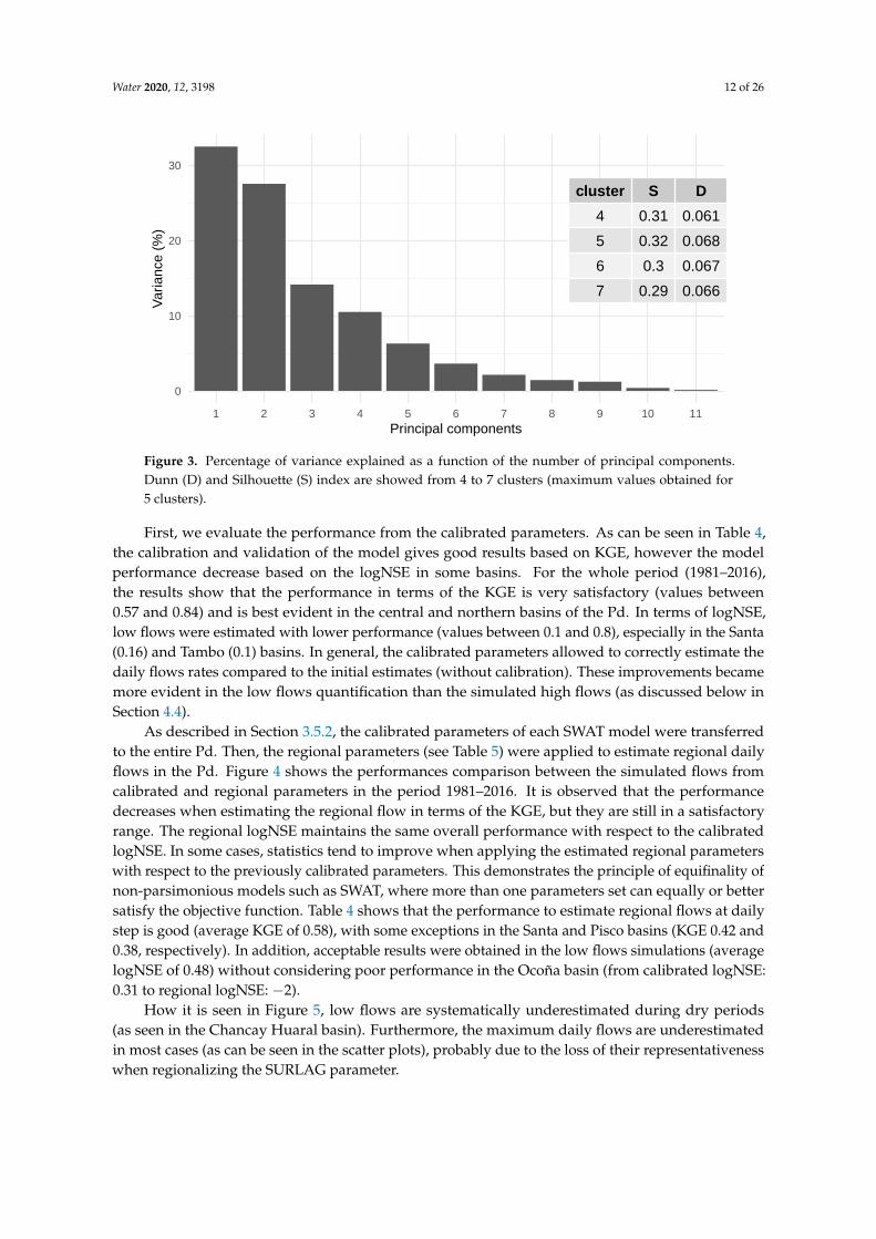
As shown in Figure 3, there is a break (elbow) that starts from the fourth principal component,which implies 4 clusters for this case. This number is adjusted from Ward’s hierarchical clustering bycomparing other situations (from 4 to 7 clusters) and validated by maximizing the Dunn and Silhouetteindexes. Finally, the 730 subbasins delimited in the Pd were grouped into five clusters. These clustersor regions characterize the particular behavior existing in the northern zone (regions 1 and 2) of thePd [7] and present at least one streamgage in each of them.

Table 3. Weightings of the variables and summary of characteristics on the five principal components.

Original VariablesPrincipal Components

PC1 PC2 PC3 PC4 PC5

Rm −0.457 −0.105 0.221 −0.040 0.147Em 0.163 0.460 0.025 0.173 0.038Qm −0.416 −0.011 0.385 0.022 0.194Rc −0.399 0.108 0.395 0.089 −0.032Ab −0.085 −0.148 −0.242 0.639 −0.202Sb −0.152 −0.316 −0.481 −0.276 0.191Zb −0.155 −0.514 0.091 −0.024 −0.096dc 0.098 0.151 0.167 −0.656 −0.339fc −0.348 0.031 −0.452 −0.215 0.222lat −0.321 0.407 −0.188 0.011 0.006

long 0.253 −0.433 0.250 −0.005 0.016

Eigenvalues 3.816 3.036 1.571 1.155 0.815Variance (%) 31.8 25.3 13.1 9.6 6.8

Cumulative variance (%) 31.8 57.1 70.2 79.8 86.6

4.2. Regional Runoff Model Performance

Five parameters of SWAT model were calibrated for 14 basins with daily flow data using theprocedure described in Section 3.4. The optimal parameters for each model were obtained by evaluatingthe model performance in a calibration period (see Table 1) and validated in two period (as indicatedin Section 3.4). Among them, the SURLAG parameter allowed to control the correct quantification ofhigh flows as much as possible, while the parameters of GWQMN and RCHRG_DP were the mostimportant to quantify correctly the flows from aquifers and to improve the simulated flows in dryperiods. The SOL_AWC and SOL_BD parameters were important to control the flow contributionfrom the subsoil.

Water 2020, 12, 3198 12 of 26

cluster

4

S

5

D

6

7

0.31

0.32

0.3

0.29

0.061

0.068

0.067

0.066

0

10

20

30

1 2 3 4 5 6 7 8 9 10 11Principal components

Var

ianc

e (%

)

Figure 3. Percentage of variance explained as a function of the number of principal components.Dunn (D) and Silhouette (S) index are showed from 4 to 7 clusters (maximum values obtained for5 clusters).

First, we evaluate the performance from the calibrated parameters. As can be seen in Table 4,the calibration and validation of the model gives good results based on KGE, however the modelperformance decrease based on the logNSE in some basins. For the whole period (1981–2016),the results show that the performance in terms of the KGE is very satisfactory (values between0.57 and 0.84) and is best evident in the central and northern basins of the Pd. In terms of logNSE,low flows were estimated with lower performance (values between 0.1 and 0.8), especially in the Santa(0.16) and Tambo (0.1) basins. In general, the calibrated parameters allowed to correctly estimate thedaily flows rates compared to the initial estimates (without calibration). These improvements becamemore evident in the low flows quantification than the simulated high flows (as discussed below inSection 4.4).

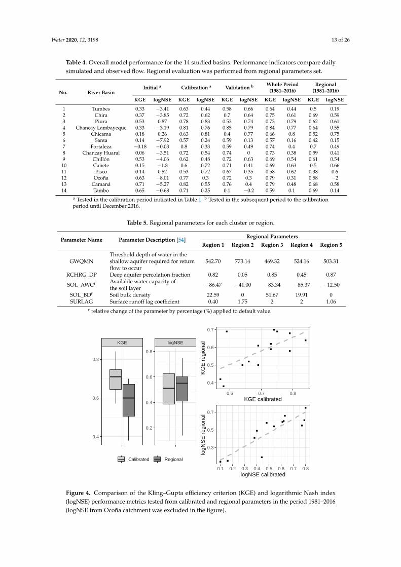
As described in Section 3.5.2, the calibrated parameters of each SWAT model were transferredto the entire Pd. Then, the regional parameters (see Table 5) were applied to estimate regional dailyflows in the Pd. Figure 4 shows the performances comparison between the simulated flows fromcalibrated and regional parameters in the period 1981–2016. It is observed that the performancedecreases when estimating the regional flow in terms of the KGE, but they are still in a satisfactoryrange. The regional logNSE maintains the same overall performance with respect to the calibratedlogNSE. In some cases, statistics tend to improve when applying the estimated regional parameterswith respect to the previously calibrated parameters. This demonstrates the principle of equifinality ofnon-parsimonious models such as SWAT, where more than one parameters set can equally or bettersatisfy the objective function. Table 4 shows that the performance to estimate regional flows at dailystep is good (average KGE of 0.58), with some exceptions in the Santa and Pisco basins (KGE 0.42 and0.38, respectively). In addition, acceptable results were obtained in the low flows simulations (averagelogNSE of 0.48) without considering poor performance in the Ocoña basin (from calibrated logNSE:0.31 to regional logNSE: −2).

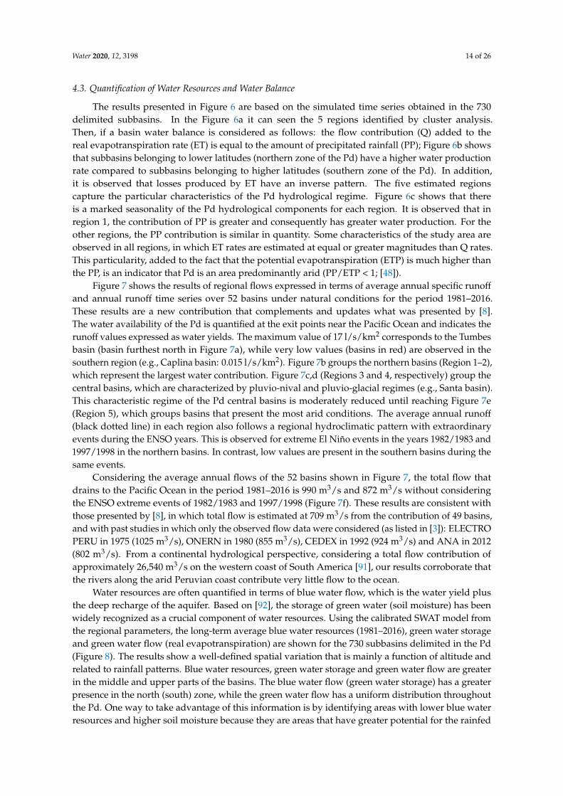
How it is seen in Figure 5, low flows are systematically underestimated during dry periods(as seen in the Chancay Huaral basin). Furthermore, the maximum daily flows are underestimatedin most cases (as can be seen in the scatter plots), probably due to the loss of their representativenesswhen regionalizing the SURLAG parameter.

Water 2020, 12, 3198 13 of 26

Table 4. Overall model performance for the 14 studied basins. Performance indicators compare dailysimulated and observed flow. Regional evaluation was performed from regional parameters set.

No. River BasinInitial a Calibration a Validation b Whole Period

(1981–2016)Regional

(1981–2016)

KGE logNSE KGE logNSE KGE logNSE KGE logNSE KGE logNSE

1 Tumbes 0.33 −3.41 0.63 0.44 0.58 0.66 0.64 0.44 0.5 0.192 Chira 0.37 −3.85 0.72 0.62 0.7 0.64 0.75 0.61 0.69 0.593 Piura 0.53 0.87 0.78 0.83 0.53 0.74 0.73 0.79 0.62 0.614 Chancay Lambayeque 0.33 −3.19 0.81 0.76 0.85 0.79 0.84 0.77 0.64 0.555 Chicama 0.18 0.26 0.63 0.81 0.4 0.77 0.66 0.8 0.52 0.756 Santa 0.14 −7.92 0.57 0.24 0.59 0.13 0.57 0.16 0.42 0.157 Fortaleza −0.18 −0.03 0.8 0.33 0.59 0.49 0.74 0.4 0.7 0.498 Chancay Huaral 0.06 −3.51 0.72 0.54 0.74 0 0.73 0.38 0.59 0.419 Chillón 0.53 −4.06 0.62 0.48 0.72 0.63 0.69 0.54 0.61 0.54

10 Cañete 0.15 −1.8 0.6 0.72 0.71 0.41 0.69 0.63 0.5 0.6611 Pisco 0.14 0.52 0.53 0.72 0.67 0.35 0.58 0.62 0.38 0.612 Ocoña 0.63 −8.01 0.77 0.3 0.72 0.3 0.79 0.31 0.58 −213 Camaná 0.71 −5.27 0.82 0.55 0.76 0.4 0.79 0.48 0.68 0.5814 Tambo 0.65 −0.68 0.71 0.25 0.1 −0.2 0.59 0.1 0.69 0.14

a Tested in the calibration period indicated in Table 1. b Tested in the subsequent period to the calibrationperiod until December 2016.

Table 5. Regional parameters for each cluster or region.

Parameter Name Parameter Description [54] Regional ParametersRegion 1 Region 2 Region 3 Region 4 Region 5

GWQMNThreshold depth of water in theshallow aquifer required for returnflow to occur

542.70 773.14 469.32 524.16 503.31

RCHRG_DP Deep aquifer percolation fraction 0.82 0.05 0.85 0.45 0.87

SOL_AWCr Available water capacity ofthe soil layer −86.47 −41.00 −83.34 −85.37 −12.50

SOL_BDr Soil bulk density 22.59 0 51.67 19.91 0SURLAG Surface runoff lag coefficient 0.40 1.75 2 2 1.06

r relative change of the parameter by percentage (%) applied to default value.

KGE logNSE

0.2

0.4

0.6

0.8

0.4

0.6

0.8

Calibrated Regional

0.4

0.5

0.6

0.7

0.6 0.7 0.8KGE calibrated

KG

E r

egio

nal

0.3

0.5

0.7

0.1 0.2 0.3 0.4 0.5 0.6 0.7 0.8logNSE calibrated

logN

SE

reg

iona

l

Figure 4. Comparison of the Kling–Gupta efficiency criterion (KGE) and logarithmic Nash index(logNSE) performance metrics tested from calibrated and regional parameters in the period 1981–2016(logNSE from Ocoña catchment was excluded in the figure).

Water 2020, 12, 3198 14 of 26

4.3. Quantification of Water Resources and Water Balance

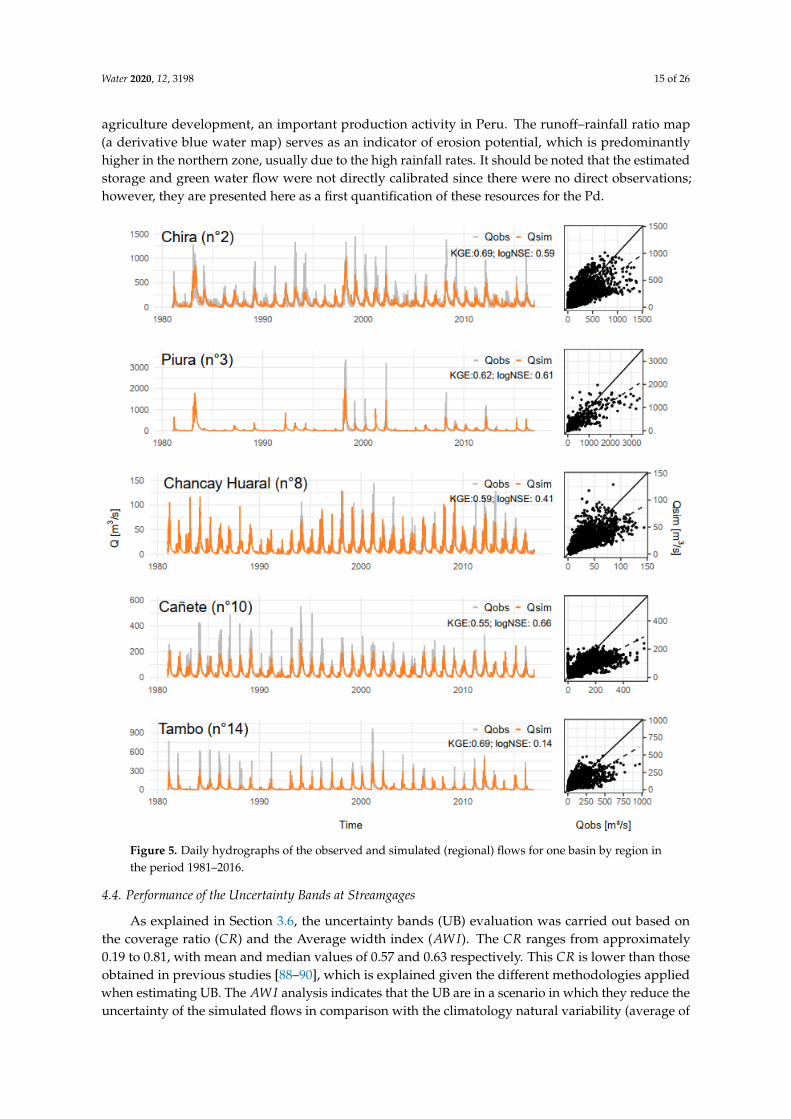
The results presented in Figure 6 are based on the simulated time series obtained in the 730delimited subbasins. In the Figure 6a it can seen the 5 regions identified by cluster analysis.Then, if a basin water balance is considered as follows: the flow contribution (Q) added to thereal evapotranspiration rate (ET) is equal to the amount of precipitated rainfall (PP); Figure 6b showsthat subbasins belonging to lower latitudes (northern zone of the Pd) have a higher water productionrate compared to subbasins belonging to higher latitudes (southern zone of the Pd). In addition,it is observed that losses produced by ET have an inverse pattern. The five estimated regionscapture the particular characteristics of the Pd hydrological regime. Figure 6c shows that thereis a marked seasonality of the Pd hydrological components for each region. It is observed that inregion 1, the contribution of PP is greater and consequently has greater water production. For theother regions, the PP contribution is similar in quantity. Some characteristics of the study area areobserved in all regions, in which ET rates are estimated at equal or greater magnitudes than Q rates.This particularity, added to the fact that the potential evapotranspiration (ETP) is much higher thanthe PP, is an indicator that Pd is an area predominantly arid (PP/ETP < 1; [48]).

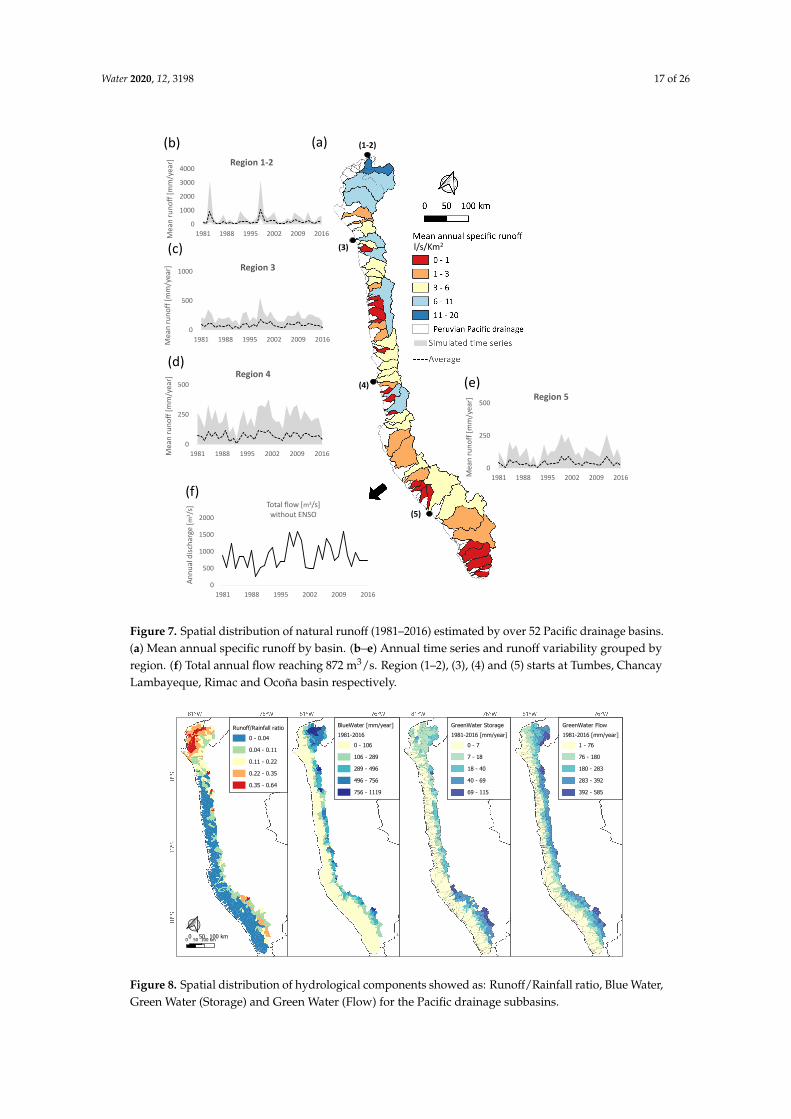
Figure 7 shows the results of regional flows expressed in terms of average annual specific runoffand annual runoff time series over 52 basins under natural conditions for the period 1981–2016.These results are a new contribution that complements and updates what was presented by [8].The water availability of the Pd is quantified at the exit points near the Pacific Ocean and indicates therunoff values expressed as water yields. The maximum value of 17 l/s/km2 corresponds to the Tumbesbasin (basin furthest north in Figure 7a), while very low values (basins in red) are observed in thesouthern region (e.g., Caplina basin: 0.015 l/s/km2). Figure 7b groups the northern basins (Region 1–2),which represent the largest water contribution. Figure 7c,d (Regions 3 and 4, respectively) group thecentral basins, which are characterized by pluvio-nival and pluvio-glacial regimes (e.g., Santa basin).This characteristic regime of the Pd central basins is moderately reduced until reaching Figure 7e(Region 5), which groups basins that present the most arid conditions. The average annual runoff(black dotted line) in each region also follows a regional hydroclimatic pattern with extraordinaryevents during the ENSO years. This is observed for extreme El Niño events in the years 1982/1983 and1997/1998 in the northern basins. In contrast, low values are present in the southern basins during thesame events.

Considering the average annual flows of the 52 basins shown in Figure 7, the total flow thatdrains to the Pacific Ocean in the period 1981–2016 is 990 m3/s and 872 m3/s without consideringthe ENSO extreme events of 1982/1983 and 1997/1998 (Figure 7f). These results are consistent withthose presented by [8], in which total flow is estimated at 709 m3/s from the contribution of 49 basins,and with past studies in which only the observed flow data were considered (as listed in [3]): ELECTROPERU in 1975 (1025 m3/s), ONERN in 1980 (855 m3/s), CEDEX in 1992 (924 m3/s) and ANA in 2012(802 m3/s). From a continental hydrological perspective, considering a total flow contribution ofapproximately 26,540 m3/s on the western coast of South America [91], our results corroborate thatthe rivers along the arid Peruvian coast contribute very little flow to the ocean.

Water resources are often quantified in terms of blue water flow, which is the water yield plusthe deep recharge of the aquifer. Based on [92], the storage of green water (soil moisture) has beenwidely recognized as a crucial component of water resources. Using the calibrated SWAT model fromthe regional parameters, the long-term average blue water resources (1981–2016), green water storageand green water flow (real evapotranspiration) are shown for the 730 subbasins delimited in the Pd(Figure 8). The results show a well-defined spatial variation that is mainly a function of altitude andrelated to rainfall patterns. Blue water resources, green water storage and green water flow are greaterin the middle and upper parts of the basins. The blue water flow (green water storage) has a greaterpresence in the north (south) zone, while the green water flow has a uniform distribution throughoutthe Pd. One way to take advantage of this information is by identifying areas with lower blue waterresources and higher soil moisture because they are areas that have greater potential for the rainfed

Water 2020, 12, 3198 15 of 26

agriculture development, an important production activity in Peru. The runoff–rainfall ratio map(a derivative blue water map) serves as an indicator of erosion potential, which is predominantlyhigher in the northern zone, usually due to the high rainfall rates. It should be noted that the estimatedstorage and green water flow were not directly calibrated since there were no direct observations;however, they are presented here as a first quantification of these resources for the Pd.

Figure 5. Daily hydrographs of the observed and simulated (regional) flows for one basin by region inthe period 1981–2016.

4.4. Performance of the Uncertainty Bands at Streamgages

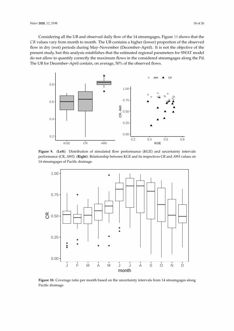
As explained in Section 3.6, the uncertainty bands (UB) evaluation was carried out based onthe coverage ratio (CR) and the Average width index (AWI). The CR ranges from approximately0.19 to 0.81, with mean and median values of 0.57 and 0.63 respectively. This CR is lower than thoseobtained in previous studies [88–90], which is explained given the different methodologies appliedwhen estimating UB. The AWI analysis indicates that the UB are in a scenario in which they reduce theuncertainty of the simulated flows in comparison with the climatology natural variability (average of

Water 2020, 12, 3198 16 of 26

AWI 0.82 in a range of 0.72 and 0.90). The satisfactory values of AWI is the result of all criterions takenin the parameters sensitivity analysis when calibrating the SWAT model (explained in Section 3.4);in this way, the values obtained do not differ much from each other, producing that simulated flowtime series variability in the bootstrapping are not extremely wide in all streamgages analyzed.

(a)

(b)

(c)

Figure 6. Water balance of Pacific subbasins. (a) Regions estimated by clustering, (b) Realevapotranspiration ratio (ET/PP) and flow ratio (Q/PP) calculated for each subbasin, (c) Hydrologicalcomponents seasonality estimated in each region. Enumerated streamgages listed in Table 1.

Figure 9 shows that the KGE and CR values show a similar variability pattern (medians of 0.60 and0.63 respectively). In addition, the CR values tend to show a positive correlation with the hydrologicalmodeling performance (KGE). In some cases, a good KGE performance can be related to different CRvalues and viceversa. In the case of AWI, independent of the KGE values, is showed values between0.7 and 0.9. There is not much variability in this index, so it is inferred that the AWI would alwaysremain in that range if more streamgages were included in the analysis.

Water 2020, 12, 3198 17 of 26

0

500

1000

1500

2000

1981 1988 1995 2002 2009 2016

An

nu

ald

isch

arge

[m3/s

] Total flow [m3/s]without ENSO

0

500

1000

1981 1988 1995 2002 2009 2016Mea

n r

un

off

[mm

/yea

r] Region 3

0

1000

2000

3000

4000

1981 1988 1995 2002 2009 2016Mea

n r

un

off

[mm

/yea

r] Region 1-2

0

250

500

1981 1988 1995 2002 2009 2016Mea

n r

un

off

[mm

/yea

r]

Region 4

0

250

500

1981 1988 1995 2002 2009 2016Mea

n r

un

off

[mm

/yea

r] Region 5

(a)

(e)

(f)

(d)

(c)

(b) (1-2)

(3)

(4)

(5)

l/s/Km2

Figure 7. Spatial distribution of natural runoff (1981–2016) estimated by over 52 Pacific drainage basins.(a) Mean annual specific runoff by basin. (b–e) Annual time series and runoff variability grouped byregion. (f) Total annual flow reaching 872 m3/s. Region (1–2), (3), (4) and (5) starts at Tumbes, ChancayLambayeque, Rimac and Ocoña basin respectively.

1981-2016

0 - 106

106 - 289

289 - 496

496 - 756

756 - 1119

BlueWater [mm/year]

1981-2016 [mm/year]

0 - 7

7 - 18

18 - 40

40 - 69

69 - 115

GreenWater StorageRunoff/Rainfall ratio

0 - 0.04

0.04 - 0.11

0.11 - 0.22

0.22 - 0.35

0.35 - 0.64

1981-2016 [mm/year]

1 - 76

76 - 180

180 - 283

283 - 392

392 - 585

GreenWater Flow

Figure 8. Spatial distribution of hydrological components showed as: Runoff/Rainfall ratio, Blue Water,Green Water (Storage) and Green Water (Flow) for the Pacific drainage subbasins.

Water 2020, 12, 3198 18 of 26

Considering all the UB and observed daily flow of the 14 streamgages, Figure 10 shows that theCR values vary from month to month. The UB contains a higher (lower) proportion of the observedflow in dry (wet) periods during May–November (December–April). It is not the objective of thepresent study, but this analysis establishes that the estimated regional parameters for SWAT modeldo not allow to quantify correctly the maximum flows in the considered streamgages along the Pd.The UB for December–April contain, on average, 50% of the observed flows.

●

●

0.2

0.4

0.6

0.8

KGE CR AWI

●

●●

●

●● ●●

●

●●

●●●

0.00

0.25

0.50

0.75

1.00

0.2 0.4 0.6 0.8KGE

CR

, AW

I

● AWI CR

Figure 9. (Left): Distribution of simulated flow performance (KGE) and uncertainty intervalsperformance (CR, AWI). (Right): Relationship between KGE and its respectives CR and AWI values on14 streamgages of Pacific drainage.

●

●●

●

●

●

●

●

●

●

●

●

0.00

0.25

0.50

0.75

1.00

J F M A M J J A S O N Dmonth

CR

Figure 10. Coverage ratio per month based on the uncertainty intervals from 14 streamgages alongPacific drainage.

Water 2020, 12, 3198 19 of 26

5. Discussion

5.1. Subjectivity in the Physical Similarity Approach by Clustering

This article presents a methodology for flow rates estimation through hydrological modelingfollowing a parameter regionalization approach. Although the SWAT model was used, the selectedregionalization method is independent of the chosen hydrological model. The regionalizationtechnique is based on the similarity approach, a method that transfers the optimal parameters setfrom calibrated hydrographic basins to similar hydrographic basins. In addition, this method isrecommended over regression and spatial proximity methods [12,16,18,23] and has shown goodperformance in hydrological modeling in arid zones [18,93]. In our work, similarity is defined bysubbasins grouping with physical and hydroclimatic characteristics that try to explain the hydrologicalbehavior. Although the PCA prior to the definition of clusters or regions eliminates much ofsubjectivity when selecting the most influential similarity variables, it should be mentioned thatthe basin characteristics most commonly available (topography, land use, soil and climate) are notsufficient to fully explain the hydrological response [17,94,95], and it is suggested to incorporateadditional basin characteristics [11]. It is likely that this includes hydrogeological characteristicsand/or basin flow regulation characteristics [30], data of difficult availability in the Pd.

5.2. Physical Implications of the Regional Parameter Set

The results of this study indicate that the five regionalized parameters can be used to producesatisfactory simulations from SWAT model in the Pd. The values shown in Table 5 are mainly relatedto the climatic conditions of the study area. In the case of the RCHRG_DP parameter, the high valuesobtained (close to 0.9) indicate that the Pd is an area where rivers are predominantly recharged byaquifers and have high potential for water harvesting [96]. Previous studies have observed thatthe SWAT model underestimates low flow rates in dry and wet periods [97,98], and consequently,the model has been modified and even coupled to other models (e.g., MODFLOW). to improve the flowcontributions from aquifers [99–102]. It is not the objective of the present study to modify the SWATsource code, but we emphasize the importance of calibrating the RCHRG_DP parameter to improve thelow flows representativeness, especially in Pd basins. In addition, this parameter sensitivity is evidentwhen it is regionalized; for example, in the Ocoña river basin, the performance of the logNSE decreasesconsiderably (see Table 4) because the value of RCHRG_DP is reduced, which causes the model tounderestimate dry periods flow. Set a suitable threshold (GWQMN) for there to be a contribution fromthe aquifer is also very important. For the Pd, these values are between 500 and 800 mm and allowedto correct the initial low flows underestimations. Although in SWAT the groundwater routine is verysimplistic, these first results suggest the need for detailed groundwater studies in the Pd and to have abetter physical interpretability of these parameters.

The parameter values of SOL_AWC and SOL_BD indicate that the Pd is characterized by anarid climate and a predominantly sandy soil (Table 1). The percentage increase of SOL_BD is relatedto lighter soils that have a lower water holding capacity than heavier or clayey soils. On the otherhand, the high rates of potential evapotranspiration (Figure 6) in arid climates generate high waterlosses to the atmosphere. The parameter SOL_AWC allows to regulate the amount of availablewater in the soil for the evapotranspiration process, and a decrease in its value corrects the initialunderestimations of SWAT model and thus improves the initial performance of the KGE (Table 4).Finally, the SURLAG parameter is important to correctly simulate the high flows according to itsphysical definition (see Table 5). From the initial SURLAG calibrated parameters, the simulated highflows generally underestimated the observed ones in most of the studied basins; however, this was afairly acceptable underestimation. Although the PISCO rainfall product does not correctly capture theintensity of the rainfall [57], one of the main factors of the low representativeness of high flows couldbe attributed when the flow is obtained from the regional SURLAG parameters (as shown in Figure 5).In the present work, greater importance was given to the water balance representation, and we indicate

Water 2020, 12, 3198 20 of 26

that for a better high flow estimation, it is recommended to condition the SWAT calibration based onindices that evaluate only the extreme flows behavior.

5.3. Conditionality of the SWAT Calibrated Model and Its Applicability

It should be noted from the beginning that hydrological models calibration is subjective andthat no automatic calibration algorithm can replace the analyst knowledge in relation to the basinhydrology and calibration problems. Therefore, the calibration and uncertainty analysis are closelylinked, and calibration results should not be presented without an uncertainty degree quantificationin the model predictions [24]. In this context, the uncertainty analyzed in this study serves as afirst approximation to evaluate the calibrated parameters set performance obtained by each region.While we use bootstrapping to increase the number of available parameters per region and to presenta more consistent analysis of the UB, we can say that the uncertainty associated with regionalizationprocess has yielded good results mainly due to the criterions used in the calibration process to reducethe equifinality of SWAT model. It is understood that more streamgages should be taken into accountfor a better analysis; however, indicating the processes that the model is not adequately representing isa “high value information” for decision makers. Based on the above, the water resources quantificationin the Pd presented here should be taken into account according to the objectives for which the SWATmodel was built. Having a regional model that estimates natural flow series and correctly representsthe Pd basins water balance is useful for identifying long-term relationships with climate variabilityand climate change impacts, and to be applied for water resource management purposes.

6. Summary and Conclusions

This study proposes a methodology for daily flows estimation in the Pacific drainage of Peru froma physically based model (SWAT). In most large-scale hydrological models, the calibration processof model parameters is critical and even more so for areas with limited availability of hydrologicaldata. A parameter transfer method was proposed based on an approach of physical similarity andclustering that divided the Pacific drainage (divided in 730 subbasins) into five regions assumedto be hydrologically homogeneous. Fourteen basins were calibrated to subsequently estimate theregional parameters based on the median of the calibrated parameters set available in each region. Asa first approximation to evaluate the methodology robustness in the parameter regionalization process,by means of statistical techniques such as bootstrapping, the uncertainty bands were derived in eachevaluated basin. The results show that the SWAT model with regional parameters can simulate theobserved flows well and correctly represent the seasonality of the hydrological cycle main components.The high rates of potential evapotranspiration on precipitation and the particular flow behavior in thenorthern zone of the Pacific drainage are equally well represented.

At the annual level, flow series pattern variability along the drainage and the total flowcontribution to the Pacific Ocean show similarity with previous studies. Certain relationships werefound between values of the calibrated parameters and physical-climatic characteristics of the basinsstudied; however, a greater analysis was not possible due to the absence of observed data to supportour assumptions. Similarly, the water resources quantification based on components of blue water,green water storage (soil moisture) and green water flow (real evapotranspiration) allowed us to obtaina better understanding of water availability and variability in the Pacific basins, which should serve asa tool for better use and management of its water resources. The evaluation of derived uncertaintybands indicated that the high flows are not correctly quantified; however, the natural variability ofobserved flow climatology is well represented. These results support the idea that flows are bettersimulated from a calibrated model than from a regionalized model. In addition, the idea is supportedthat the best way to handle the problem of rainfall–runoff modeling in uncalibrated basins would beto install a streamgage.

Water 2020, 12, 3198 21 of 26

The present study adds to the research efforts in the hydrological modeling field at the regionalscale that have been carried out in recent years on the Peruvian Pacific drainage. A first stepis presented to expand the use and development of physical bases hydrological models for theirapplication at a regional scale, and the presented parameters transfer approach is promising to estimateSWAT parameters in areas with scarce hydrological data in Peru. Future studies will be dedicatedto investigating the flow rates sensitivity in a context of climate change and exploring calibrationtechniques in hydrological modeling to correctly estimate annual maximum daily flows.

Supplementary Materials: The metadata is available online at: https://figshare.com/articles/dataset/SWAT_Pacifico_main_outputs/13236941.

Author Contributions: Conceptualization, F.A.A.-V., W.S.L.-C.; Formal analysis, F.A.A.-V., W.S.L.-C.;Investigation, F.A.A.-V., W.S.L.-C.; Methodology, F.A.A.-V., W.S.L.-C.; Software, F.A.A.-V., Writing—review& editing, F.A.A.-V., W.S.L.-C., Supervision, F.A.A.-V., W.S.L.-C. All authors have read and agreed to the publishedversion of the manuscript.

Funding: This research was funded by the Swiss Agency for Development and Cooperation (SDC) andimplemented by South South North (SSN) and Libélula Institute of Global Change under the direction of theEnvironment Ministry of Peru (Ministerio del Ambiente—MINAM).

Acknowledgments: We thank all the support offered in the framework of the project “Apoyo a la Gestión delCambio Climático Segunda Fase (período 2019–2021)”. Likewise, we thank the technical-scientific supportprovided and the hydrological data shared by the Hydrology Department of the National Service of Meteorologyand Hydrology of Peru (SENAMHI).

Conflicts of Interest: The authors declare no conflict of interest.

References

1. Garreaud, R.; Vuille, M.; Compagnucci, R.; Marengo, J. Present-day South American climate.Paleogeogr. Palaeoclimatol. Paleoecol. 2009, 281, 180–195. [CrossRef]

2. Ruiz, R.; Torres, H.; Aguirre, M. Delimitación y Codificación de Unidades Hidrográficas del Perú; AutoridadNacional del Agua—Ministerio de Agricultura: Lima, Perú, 2008.

3. ANA. Recursos Hídricos en el Perú; Technical Report; Ministerio de Agricultura: Lima, Perú, 2012.4. PRB. World Population Data Sheet (Population Reference Bureau); PRB: Washington, DC, USA, 2020.5. FAO. FAO Statistical Yearbook 2013: World Food and Agriculture; FAO: Rome, Italy, 2013.6. Lavado, W.S.; Ronchail, J.; Labat, D.; Espinoza, J.C.; Guyot, J.L. Basin-scale analysis of rainfall and runoff in

Peru (1969–2004): Pacific, Titicaca and Amazonas drainages. Hydrol. Sci. J. 2012, 57, 625–642, [CrossRef]7. Rau, P.; Bourrel, L.; Labat, D.; Melo, P.; Dewitte, B.; Frappart, F.; Lavado, W.; Felipe, O. Regionalization of

rainfall over the Peruvian Pacific slope and coast. Int. J. Climatol. 2017, 37, 143–158. [CrossRef]8. Rau, P.; Bourrel, L.; Labat, D.; Ruelland, D.; Frappart, F.; Lavado, W.; Dewitte, B.; Felipe, O.

Assessing multidecadal runoff (1970–2010) using regional hydrological modelling under data and waterscarcity conditions in Peruvian Pacific catchments. Hydrol. Process. 2019, 33, 20–35, [CrossRef]

9. Seiller, G.; Anctil, F.; Perrin, C. Multimodel evaluation of twenty lumped hydrological models undercontrasted climate conditions. Hydrol. Earth Syst. Sci. 2012, 16,1171–1189. [CrossRef]

10. Beck, H.E.; van Dijk, A.I.; De Roo, A.; Miralles, D.G.; McVicar, T.R.; Schellekens, J.; Bruijnzeel, L.A.Global-scale regionalization of hydrologic model parameters. Water Resour. Res. 2016, 52, 3599–3622.[CrossRef]

11. Oudin, L.; Kay, A.; Andréassian, V.; Perrin, C. Are seemingly physically similar catchments trulyhydrologically similar? Water Resour. Res. 2010, 46, [CrossRef]

12. Oudin, L.; Andréassian, V.; Perrin, C.; Michel, C.; Le Moine, N. Spatial proximity, physical similarity,regression and ungaged catchments: A comparison of regionalization approaches based on 913 Frenchcatchments. Water Resour. Res. 2008, 44, 1–15, [CrossRef]

13. Stoll, S.; Weiler, M. Explicit simulations of stream networks to guide hydrological modelling in ungaugedbasins. Hydrol. Earth Syst. Sci. 2010, 14, 1435–1448, [CrossRef]

Water 2020, 12, 3198 22 of 26

14. Samuel, J.; Coulibaly, P.; Metcalfe, R.A. Estimation of continuous streamflow in Ontario ungauged basins:comparison of regionalization methods. J. Hydrol. Eng. 2011, 16, 447–459, [CrossRef]

15. Parajka, J.; Viglione, A.; Rogger, M.; Salinas, J.; Sivapalan, M.; Blöschl, G. Comparative assessment ofpredictions in ungauged basins–Part 1: Runoff hydrograph studies. Hydrol. Earth Syst. Sci. Discuss. 2013, 10,[CrossRef]

16. Razavi, T.; Coulibaly, P. Streamflow Prediction in Ungauged Basins: Review of Regionalization Methods.J. Hydrol. Eng. 2013, 18, 958–975, [CrossRef]

17. Merz, R.; Blöschl, G. Regionalisation of catchment model parameters. J. Hydrol. 2004, 287, 95–123. [CrossRef]18. Parajka, J.; Merz, R.; Blöschl, G. A comparison of regionalisation methods for catchment model parameters.

Hydrol. Earth Syst. Sci. 2005, 9, 157–171. [CrossRef]19. McIntyre, N.; Lee, H.; Wheater, H.; Young, A.; Wagener, T. Ensemble predictions of runoff in ungauged

catchments. Water Resour. Res. 2005, 41. [CrossRef]20. Bárdossy, A. Calibration of hydrological model parameters for ungauged catchments. Eur. Geosci. Union

2007, 11, 703–710, [CrossRef]21. Zhang, Y.; Chiew, F.H. Relative merits of different methods for runoff predictions in ungauged catchments.

Water Resour. Res. 2009, 45. [CrossRef]22. Merz, R.; Blöschl, G.; Parajka, J.D. Regionalization methods in rainfall-runoff modelling using large

catchment samples. IAHS Publ. 2006, 307, 117.23. Arsenault, R.; Brissette, F.P. Continuous streamflow prediction in ungauged basins: The effects of equifinality

and parameter set selection on uncertainty in regionalization approaches. J. Am. Water Resour. Assoc. 2014,50, 6135–6153, [CrossRef]

24. Abbaspour, K.C.; Rouholahnejad, E.; Vaghefi, S.; Srinivasan, R.; Yang, H.; Kløve, B. A continental-scalehydrology and water quality model for Europe: Calibration and uncertainty of a high-resolution large-scaleSWAT model. J. Hydrol. 2015, 524, 733–752, [CrossRef]

25. Arnold, J.G.; Srinivasan, R.; Muttiah, R.S.; Williams, J.R. Large area hydrologic modeling and assessmentpart I: Model development 1. JAWRA J. Am. Water Resour. Assoc. 1998, 34, 73–89. [CrossRef]

26. Gitau, M.W.; Chaubey, I. Regionalization of SWAT model parameters for use in ungauged watersheds. Water2010, 2, 849–871, [CrossRef]

27. Swain, J.B.; Patra, K.C. Streamflow estimation in ungauged catchments using regionalization techniques.J. Hydrol. 2017, 554, 420–433, [CrossRef]

28. Van Liew, M.W.; Mittelstet, A.R. Comparison of three regionalization techniques for predicting streamflowin ungaged watersheds in nebraska, USA using SWAT model. Int. J. Agric. Biol. Eng. 2018, 11, 110–119,[CrossRef]

29. Choubin, B.; Solaimani, K.; Rezanezhad, F.; Habibnejad Roshan, M.; Malekian, A.; Shamshirband, S. Streamflowregionalization using a similarity approach in ungauged basins: Application of the geo-environmental signaturesin the Karkheh River Basin, Iran. Catena 2019, 182, 104128, doi:10.1016/j.catena.2019.104128. [CrossRef]

30. Pagliero, L.; Bouraoui, F.; Diels, J.; Willems, P.; McIntyre, N. Investigating regionalization techniquesfor large-scale hydrological modelling. J. Hydrol. 2019, 570, 220–235, doi:10.1016/j.jhydrol.2018.12.071.[CrossRef]

31. Molina, L.A.U. Validacion del Modelo Hidrologico SWAT, con interfaz Arcview, en la cuenca alta del rioChama, estado Merida. Rev. For. Venez. 2005, 49, 105–106.

32. Stehr, A.; Debels, P.; Romero, F.; Alcayaga, H. Hydrological modelling with SWAT under conditions oflimited data availability: Evaluation of results from a Chilean case study. Hydrol. Sci. J. 2008, 53, 588–601.[CrossRef]

33. Stehr, A.; Debels, P.; Arumi, J.L.; Romero, F.; Alcayaga, H. Combining the Soil and Water Assessment Tool(SWAT) and MODIS imagery to estimate monthly flows in a data-scarce Chilean Andean basin. Hydrol. Sci. J.2009, 54, 1053–1067. [CrossRef]

34. Barrios, A.G.; Urribarri, L.A. Aplicación del modelo Swat en los Andes venezolanos: Cuenca alta del ríoChama. Rev. Geográfica Venez. 2010, 51, 11–29.

35. Alarcon, V.J.; Alcayaga, H.; Álvarez, E. Hydrological modeling of an ungauged watershed in SouthernAndes. In AIP Conference Proceedings; AIP Publishing LLC: Melville, NY, USA, 2015; Volume 1702, p. 190003.

Water 2020, 12, 3198 23 of 26

36. Yacoub, C.; Pérez-Foguet, A. Assessment of terrain slope influence in SWAT modeling of Andean watersheds.EGUGA 2009,11, 6381.

37. Uribe, N.; Quintero, M.; Valencia, J. Aplicación del Modelo Hidrológico SWAT (Soil and Water Assessment Tool)a la Cuenca del Río Cañete (SWAT); Technical Report; International Center for Tropical Agriculture: Cali,Colombia, 2013.

38. Lavado Casimiro, W.S.; Labat, D.; Guyot, J.L.; Ardoin-Bardin, S. Assessment of climate change impacts onthe hydrology of the Peruvian Amazon–Andes basin. Hydrol. Process. 2011, 25, 3721–3734. [CrossRef]

39. Andres, N.; Vegas Galdos, F.; Lavado Casimiro, W.S.; Zappa, M. Water resources and climate change impactmodelling on a daily time scale in the Peruvian Andes. Hydrol. Sci. J. 2014, 59, 2043–2059. [CrossRef]

40. Zulkafli, Z.; Buytaert, W.; Manz, B.; Rosas, C.V.; Willems, P.; Lavado-Casimiro, W.; Guyot, J.L.; Santini, W.Projected increases in the annual flood pulse of the Western Amazon. Environ. Res. Lett. 2016, 11, 014013.[CrossRef]

41. Olsson, T.; Kämäräinen, M.; Santos, D.; Seitola, T.; Tuomenvirta, H.; Haavisto, R.; Lavado-Casimiro, W.Downscaling climate projections for the Peruvian coastal Chancay-Huaral Basin to support river dischargemodeling with WEAP. J. Hydrol. Reg. Stud. 2017, 13, 26–42, [CrossRef]

42. Lavado Casimiro, W.S.; Labat, D.; Guyot, J.L.; Ronchail, J.; Ordonez, J.; others. TRMM rainfall dataestimation over the Peruvian Amazon-Andes basin and its assimilation into a monthly water balance model.In New Approaches to Hydrological Prediction in Datasparse Regions, Proceedings of Symposium HS; IAHS Press:Hyderabad, India, 2009; Volume 2, pp. 207–216.

43. Zulkafli, Z.; Buytaert, W.; Onof, C.; Manz, B.; Tarnavsky, E.; Lavado, W.; Guyot, J.L. A comparativeperformance analysis of TRMM 3B42 (TMPA) versions 6 and 7 for hydrological applications overAndean–Amazon river basins. J. Hydrometeorol. 2014, 15, 581–592. [CrossRef]

44. Zubieta, R.; Getirana, A.; Espinoza, J.C.; Lavado, W. Impacts of satellite-based precipitation datasets onrainfall–runoff modeling of the Western Amazon basin of Peru and Ecuador. J. Hydrol. 2015, 528, 599–612.[CrossRef]

45. Strauch, M.; Kumar, R.; Eisner, S.; Mulligan, M.; Reinhardt, J.; Santini, W.; Vetter, T.; Friesen, J. Adjustment ofglobal precipitation data for enhanced hydrologic modeling of tropical Andean watersheds. Clim. Chang.2017, 141, 547–560. [CrossRef]

46. Satgé, F.; Ruelland, D.; Bonnet, M.P.; Molina, J.; Pillco, R. Consistency of satellite precipitation estimatesin space and over time compared with gauge observations and snow-hydrological modelling in the lakeTiticaca region. Hydrol. Earth Syst. Sci. 2018, 1–41.

47. De Reparaz, G. Los Ríos de la Zona árida Peruana; Universidad de Piura: Piura, Perú, 2013.48. Rau, P.; Bourrel, L.; Labat, D.; Frappart, F.; Ruelland, D.; Lavado, W.; Dewitte, B.; Felipe, O. Hydroclimatic

change disparity of Peruvian Pacific drainage catchments. Theor. Appl. Climatol. 2018, 134, 139–153,[CrossRef]

49. Lavado, W.; Espinoza, J.C. Impactos de El Niño y La Niña en las lluvias del Perú (1965–2007). Rev. Bras.Meteorol. 2014, 29, 171–182. [CrossRef]

50. Bourrel, L.; Rau, P.; Dewitte, B.; Labat, D.; Lavado, W.; Coutaud, A.; Vera, A.; Alvarado, A.; Ordoñez, J.Low-frequency modulation and trend of the relationship between ENSO and precipitation along the northernto centre Peruvian Pacific coast. Hydrol. Process. 2015, 29, 1252–1266. [CrossRef]

51. Sanabria, J.; Bourrel, L.; Dewitte, B.; Frappart, F.; Rau, P.; Solis, O.; Labat, D. Rainfall along the coast of Peruduring strong El Niño events. Int. J. Climatol. 2018, 38, 1737–1747. [CrossRef]

52. Vargas, P. El Cambio Climático y sus Efectos en el Perú; Banco Central de Reserva del Perú: Lima, Perú, 2009.53. Arnold, J.; Allen, P. Estimating hydrologic budgets for three Illinois watersheds. J. Hydrol. 1996, 176, 57–77.

[CrossRef]54. Neitsch, S.; Arnold, J.; Kiniry, J.; Williams, J. Soil & Water Assessment Tool Theoretical Documentation Version

2009; Texas Water Resour Inst.: Forney, TX, USA, 2011; pp. 1–647.55. Chaplot, V. Impact of DEM mesh size and soil map scale on SWAT runoff, sediment, and NO3–N loads

predictions. J. Hydrol. 2005, 312, 207–222. [CrossRef]56. Bormann, H.; Breuer, L.; Gräff, T.; Huisman, J.; Croke, B. Assessing the impact of land use change on

hydrology by ensemble modelling (LUCHEM) IV: Model sensitivity to data aggregation and spatial (re-)distribution. Adv. Water Resour. 2009, 32, 171–192. [CrossRef]

Water 2020, 12, 3198 24 of 26

57. Aybar, C.; Fernández, C.; Huerta, A.; Lavado, W.; Vega, F.; Felipe-Obando, O. Construction of ahigh-resolution gridded rainfall dataset for Peru from 1981 to the present day. Hydrol. Sci. J. 2019,65, 770–785. [CrossRef]

58. Huerta, A.; Aybar, C.; Lavado, W. PISCO Tem-Perature v.1.1.; Technical Report; SENAMHI: Lima, Perú, 2018.59. Lehner, B.; Verdin, K.; Jarvis, A. New global hydrography derived from spaceborne elevation data. Eos Trans.

Am. Geophys. Union 2008, 89, 93–94. [CrossRef]60. Bontemps, S.; Defourny, P.; Radoux, J.; Van Bogaert, E.; Lamarche, C.; Achard, F.; Mayaux, P.; Boettcher, M.;

Brockmann, C.; Kirches, G.; et al. Consistent global land cover maps for climate modelling communities:Current achievements of the ESA’s land cover CCI. In Proceedings of the ESA Living Planet Symposium,Edimburgh, UK, 9–13 September 2013; pp. 9–13.

61. FAO-UNESCO. Soil Map of the World; Technical Report South America; FAO-UNESCO: Rome, Italy, 1971.62. Dile, Y.T.; Daggupati, P.; George, C.; Srinivasan, R.; Arnold, J. Introducing a new open source GIS user

interface for the SWAT model. Environ. Model. Softw. 2016, 85, 129–138. [CrossRef]63. Luo, Y.; Su, B.; Yuan, J.; Li, H.; Zhang, Q. GIS techniques for watershed delineation of SWAT model in plain

polders. Procedia Environ. Sci. 2011, 10, 2050–2057. [CrossRef]64. Hargreaves, G.H.; Samani, Z.A. Reference crop evapotranspiration from temperature. Appl. Eng. Agric.

1985, 1, 96–99. [CrossRef]65. Priestley, C.H.B.; Taylor, R. On the assessment of surface heat flux and evaporation using large-scale

parameters. Mon. Weather. Rev. 1972, 100, 81–92. [CrossRef]66. Monteith, J. Evaporation and environment. The state and movement of water in living organisms.

In Symposium of the Society of Experimental Biology; Cambridge Univ. Press: Cambridge, UK, 1965; Volume 19,pp. 205–234.

67. Aouissi, J.; Benabdallah, S.; Chabaane, Z.L.; Cudennec, C. Evaluation of potential evapotranspirationassessment methods for hydrological modelling with SWAT—Application in data-scarce rural Tunisia.Agric. Water Manag. 2016, 174, 39–51. [CrossRef]

68. Arnold, J.G.; Moriasi, D.N.; Gassman, P.W.; Abbaspour, K.C.; White, M.J.; Srinivasan, R.; Santhi, C.;Harmel, R.; Van Griensven, A.; Van Liew, M.W.; et al. SWAT: Model use, calibration, and validation.Trans. ASABE 2012, 55, 1491–1508. [CrossRef]

69. Abbaspour, K.C.; Vaghefi, S.A.; Srinivasan, R. A Guideline for Successful Calibration and UncertaintyAnalysis for Soil and Water Assessment: A Review of Papers from the 2016 International SWAT Conference.Water 2017, 10, 6, [CrossRef]

70. Gupta, H.V.; Kling, H.; Yilmaz, K.K.; Martinez, G.F. Decomposition of the mean squared error and NSEperformance criteria: Implications for improving hydrological modelling. J. Hydrol. 2009, 377, 80–91,[CrossRef]

71. Chilkoti, V.; Bolisetti, T.; Balachandar, R. Multi-objective autocalibration of SWAT model for improved lowflow performance for a small snowfed catchment. Hydrol. Sci. J. 2018, 63, 1482–1501, [CrossRef]

72. Saraiva, A.M.; Masih, I.; Uhlenbrook, S.; Jewitt, G.P.; Van der Zaag, P. Improved process representation inthe simulation of the hydrology of a meso-scale semi-arid catchment. Water 2018, 10, 1549. [CrossRef]

73. Siderius, C.; Biemans, H.; Kashaigili, J.J.; Conway, D. Going local: Evaluating and regionalizing a globalhydrological model’s simulation of river flows in a medium-sized East African basin. J. Hydrol. Reg. Stud.2018, 19, 349–364. [CrossRef]

74. Zambrano-Bigiarini, M. hydroGOF: Goodness-of-Fit Functions for Comparison of Simulated and ObservedHydrological Time Series R Package Version 0.4-0. 2020. Available online: https://cran.r-project.org/web/packages/hydroGOF/hydroGOF.pdf (accessed on 4 May 2020).

75. Confesor, R.B.; Whittaker, G. Multi-Objective Automatic Calibration of a Semi-Distributed Watershed Modelusing Pareto Ordering Optimization and Genetic Algorithm. In Proceedings of the 2006 ASAE AnnualMeeting. American Society of Agricultural and Biological Engineers, Portland, OR, USA, 9–12 July 2006; p. 1.

76. Zhang, Z.; Wagener, T.; Reed, P.; Bhushan, R. Reducing uncertainty in predictions in ungauged basins bycombining hydrologic indices regionalization and multiobjective optimization. Water Resour. Res. 2008.[CrossRef]

Water 2020, 12, 3198 25 of 26

77. Ercan, M.B.; Goodall, J.L. Design and implementation of a general software library for using NSGA-II withSWAT for multi-objective model calibration. Environ. Model. Softw. 2016, 84, 112–120, [CrossRef]

78. Ching-Shih Tsou. nsga2R: Elitist Non-dominated Sorting Genetic Algorithm Based on R. 2013. Availableonline: https://cran.r-project.org/web/packages/nsga2R/nsga2R.pdf (accessed on 25 May 2020).

79. Hannah, D.M.; Kansakar, S.R.; Gerrard, A.; Rees, G. Flow regimes of Himalayan rivers of Nepal: nature andspatial patterns. J. Hydrol. 2005, 308, 18–32. [CrossRef]

80. Ward, J.H. Hierarchical grouping to optimize an objective function. J. Am. Stat. Assoc. 1963, 58, 236–244.[CrossRef]

81. Jolliffe, I.T.; Cadima, J. Principal component analysis: A review and recent developments. Philos. Trans. R.Soc. Math. Phys. Eng. Sci. 2016, 374, 20150202. [CrossRef]

82. Rao, A.R.; Srinivas, V. Regionalization of watersheds by hybrid-cluster analysis. J. Hydrol. 2006, 318, 37–56.[CrossRef]

83. Liu, Y.; Li, Z.; Xiong, H.; Gao, X.; Wu, J. Understanding of internal clustering validation measures.In Proceedings of the 2010 IEEE International Conference on Data Mining, ICDM; IEEE: New York, NY, USA,2010; pp. 911–916, [CrossRef]

84. Chavoshi, S.; Azmin Sulaiman, W.; Saghafian, B.; Sulaiman, M.N.; Latifah, A. Soft and hard clusteringmethods for delineation of hydrological homogeneous regions in the southern strip of the Caspian Sea Watershed. J. Flood Risk Manag. 2012, 5, 282–294. [CrossRef]

85. Brock, G.; Pihur, V.; Datta, S.; Datta, S.; Brock, M.G.; Biobase, S. clValid, an R package for cluster validation.J. Stat. Softw., 2020, 25, 1–22.

86. Xie, Z.; Yuan, F.; Duan, Q.; Zheng, J.; Liang, M.; Chen, F. Regional Parameter Estimation of the VIC LandSurface Model: Methodology and Application to River Basins in China. J. Hydrometeorol. 2007, 8, 447–468,[CrossRef]

87. Efron, B. Bootstrap methods: Another look at the jackknife. In Breakthroughs in Statistics; Springer: New York,NY, USA, 1992; pp. 569–593.

88. Bourgin, F.; Andréassian, V.; Perrin, C.; Oudin, L. Transferring global uncertainty estimates from gauged toungauged catchments. Hydrol. Earth Syst. Sci. 2015, 19, 2535–2546, [CrossRef]

89. Bock, A.R.; Farmer, W.H.; Hay, L.E. Quantifying uncertainty in simulated streamflow and runoff from acontinental-scale monthly water balance model. Adv. Water Resour. 2018, 122, 166–175, [CrossRef]

90. Levin, S.; Farmer, W. Evaluation of Uncertainty Intervals for Daily, Statistically Derived Streamflow Estimatesat Ungaged Basins Across the Continental U.S. Water 2020, 12, 1390, [CrossRef]

91. Milliman, J.D.; Farnsworth, K.L. River Discharge to the Coastal Ocean: A Global Synthesis; Cambridge UniversityPress: Cambridge, UK, 2013.

92. Falkenmark, M.; Rockström, J. The new blue and green water paradigm: Breaking new ground for waterresources planning and management. J. Water Resour. Plan. Manag. 2006, 132, 129–132. [CrossRef]

93. Reichl, J.; Western, A.; McIntyre, N.; Chiew, F. Optimization of a similarity measure for estimating ungaugedstreamflow. Water Resour. Res. 2009, 45.:10.1029/2008WR007248. [CrossRef]

94. Merz, R.; Blöschl, G. Flood frequency regionalisation—spatial proximity vs. catchment attributes. J. Hydrol.2005, 302, 283–306. [CrossRef]

95. Merz, R.; Blöschl, G.; Parajka, J. Spatio-temporal variability of event runoff coefficients. J. Hydrol. 2006,331, 591–604. [CrossRef]

96. Sood, A.; Muthuwatta, L.; McCartney, M. A SWAT evaluation of the effect of climate change on the hydrologyof the Volta River basin. Water Int. 2013, 38, 297–311, [CrossRef]

97. Chu, T.; Shirmohammadi, A. Evaluation of the SWAT model’s hydrology component in the piedmontphysiographic region of Maryland. Trans. ASAE 2004, 47, 1057. [CrossRef]

98. Pfannerstill, M.; Guse, B.; Fohrer, N. A multi-storage groundwater concept for the SWAT model to emphasizenonlinear groundwater dynamics in lowland catchments. Hydrol. Process. 2014, 28, 5599–5612. [CrossRef]

99. Luo, Y.; Arnold, J.; Allen, P.; Chen, X. Hydrology and Earth System Sciences Baseflow simulation usingSWAT model in an inland river basin in Tianshan Mountains, Northwest China. Hydrol. Earth Syst. Sci. 2012,16, 1259–1267, [CrossRef]

100. Izady, A.; Davary, K.; Alizadeh, A.; Ziaei, A.N.; Akhavan, S.; Alipoor, A.; Joodavi, A.; Brusseau, M.L.Conceptualisation et modélisation hydrogéologique de la plain semi-aride et agricole de Neishaboor (Iran)en utilisant le modèle distribué SWAT. Hydrogeol. J. 2014, 23, 47–68, [CrossRef]

Water 2020, 12, 3198 26 of 26

101. Dowlatabadi, S.; Ali Zomorodian, S.M. Conjunctive simulation of surface water and groundwater usingSWAT and MODFLOW in Firoozabad watershed. KSCE J. Civ. Eng. 2016, 20, 485–496, [CrossRef]

102. Shao, G.; Zhang, D.; Guan, Y.; Xie, Y.; Huang, F. Application of SWAT model with a modified groundwatermodule to the semi-arid Hailiutu River catchment, northwest China. Sustainability 2019, 11, 2031, [CrossRef]

Publisher’s Note: MDPI stays neutral with regard to jurisdictional claims in published maps and institutionalaffiliations.

© 2020 by the authors. Licensee MDPI, Basel, Switzerland. This article is an open accessarticle distributed under the terms and conditions of the Creative Commons Attribution(CC BY) license (http://creativecommons.org/licenses/by/4.0/).