Embed Size (px)
Citation preview

Regional Needs and Instrumentation for CO2 Observations
Britton Stephens, NCAR ASP Colloquium, June 11, 2007

Outline
• Background– Regional Needs
• CO2 Measurement Techniques
– AIRCOA Example– Sources of potential bias
• Regional Applications of in situ CO2 Observations

Carbon cycle science as a field began with the careful observational work of Dave Keeling
Keeling, C.D., Rewards and penalties of monitoring the earth, Annu. Rev. Energy Environ., 23, 25-82, 1998.

2
1
0
-1
-2
Pg
C /
yr
Background CO2 measurements define global trends and loosely constrain continental-scale fluxes
Expected from fossil fuel emissions
TransCom 3 Study Fluxes60
30
0
-30
-60
Bill
ion
$
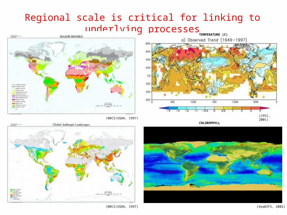
Regional scale is critical for linking to underlying processes
(NRCS/USDA, 1997)
(NRCS/USDA, 1997) (SeaWIFS, 2002)
CHLOROPHYLL
TEMPERATURE (C)
(IPCC, 2001)

TURC/NDVI Biosphere Takahashi Ocean EDGAR Fossil Fuel
[U. Karstens and M. Heimann, 2001]
Continental mixed-layer CO2 is highly variable
NWR Mean Diurnal Cycle and Hourly Variability June 2006
Rocky RACCOON CO2 Concentrations April 2007

Flux footprint, in ppm(GtCyr-1)-1, for a 106 km2 chaparral region in the U.S. Southwest (Gloor et al., 1999).
Using high frequency data makes signals bigger, but the annual-mean signals are still very small:
To measure 0.2 GtCyr-1 source/sink to +/- 25% need to measure regional annual mean gradients to 0.1-0.2 ppm

[ Recommendations of the 13th WMO/IAEA Meeting of Experts on Carbon Dioxide Concentration and Related Tracers Measurement Techniques, http://www.wmo.int/pages/prog/arep/gaw/documents/gaw168.pdf ]
1 instrument over time in the field
1 instrument over time in the lab
1 instrument over several seconds
2 instruments over time in the field
Important Definitions

Absolute Measurement Techniques: Manometric and Gravimetric
NOAA/CMDL Manometer:
Reproducibility of 0.06 ppm
(C. Zhao et al., 1997)Keeling manometer has run since ’50s

Relative Measurement Techniques: Non-dispersive Infrared (NDIR) Spectroscopy
(from www.tsi.com)
• Broadband IR radiation filtered for 4.26 um
• Cooled emitter and detector
• Pulsed emitter or chopper wheel
• 1 or 2 detection cells
Advantages: Robust, precise, affordable
Disadvantages: Non-linear; sensitivity to pressure, temperature, and optical conditions; pressure broadening

LiCor, Inc. CO2 AnalyzerCMDL Flask Analysis System

Cavity Ringdown Spectroscopy (CRDS)
Advantages: Precise, extremely stable
Disadvantages: Somewhat more expensive, relatively new

Relative measurements require calibration gases tied to a common scale
NOAA/CMDL scheme for
propagation of WMO CO2 scale:
For NDIR, generally 4 points needed for 0.1 ppm comparability
Recalibration needed ~ every 3 years due to drift

NCAR CO2 and O2/N2 Calibration Facility
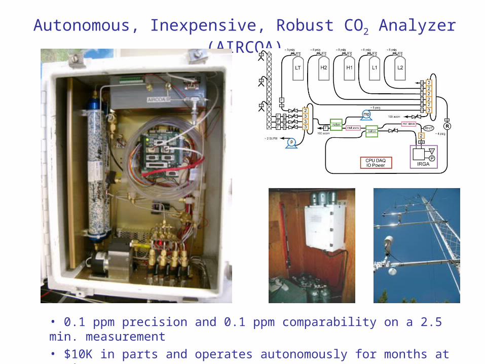
Autonomous, Inexpensive, Robust CO2 Analyzer (AIRCOA)
• 0.1 ppm precision and 0.1 ppm comparability on a 2.5 min. measurement
• $10K in parts and operates autonomously for months at a time

Potential source of bias AIRCOA solutionRelating to WMO CO2 Scale Dedicated CO2 and O2 calibration transfer facility
Short-term IRGA noise Average for 2 minutes to get better than 0.1 ppm precision
Drift in IRGA sensitivity 4-hourly 4-point calibrations and 30-minute 1-point calibrations
IRGA pressure sensitivity Automated 4-hourly pressure sensitivity measurements
IRGA temperature sensitivity 30-minute 1-point calibrations, temperature control at some sites
Incomplete drying of air Slow enough flow (100 sccm), two 96” Nafion driers, downstream humidity sensor to verify performance
Drying system altering CO2 Continuous flows and pressures through Nafions and run surveillance gas through entire system
Incomplete flushing of cell and dead volumes
Fast enough flow (100 sccm), alternate calibration sequence low‑to-high / high-to-low to look for effects
Leaks through fittings, solenoid valves, and pumps
Automated 8-hourly positive pressure leak-down and 4-hourly ambient pressure leak-up checks
Pressure broadening without Ar Use calibration gases made with real air
Fossil CO2 in calibration gases and different field and lab 13C sensitivities
Laboratory tests limit current effect to 0.05 ppm, long-term plans to use cylinders with natural CO2
Regulator temperature effects Tests suggest effect is negligible, but could be regulator dependent
Regulator flushing effects Repeat calibration tests suggest the effect is negligible
Whole-system diagnostics and comparability verification
Long-term surveillance tank analyzed every 8 hours, co-location with other programs, rotating cylinders, and laboratory comparisons
Delay in diagnosis of errors Near real-time data acquisition, processing, and dissemination

Automated web-based output
http://raccoon.ucar.edu

The NOAA flasks have a mean offset and standard deviation relative to our measurements of 0.01 ppm +/- 0.18 ppm.
Field Surveillance Tanks
NOAA GMD Flask Comparisons
Mean offsets (and standard deviations) of these measurements from the laboratory-assigned values were: ‑0.08 (+/- 0.11), -0.07 (+/- 0.11), and -0.01 (+/- 0.07) ppm at the three sites.

Map of existing North American continuous well-calibrated CO2 measurements. Colors denote measuring group, with Rocky RACCOON sites in Red. Courtesy of S. Richardson (http://ring2.psu.edu).
Map showing existing Rocky RACCOON sites (red), proposed new sites (purple), and potential future sites (gray).
Continuous, well-calibrated CO2 measurements across North America
Towers over 650 feet AGL in U.S.

NWR – SPL = -2.1 ppm CO2
HYSPLIT back-trajectory calculation for the afternoon of June 17, 2006 (6 PM LT), over topography (GoogleEarth Pro). The EDAS 40 km meteorology used for this simulation predicts that air which passed near SPL at 2 PM LT reached NWR at 6 PM LT. Using the observed CO2 difference and the model transit time of 260 minutes, the model boundary-layer heights of 2000 m at SPL and 1878 m at NWR, an average atmospheric pressure of 60 kPa over this column, and a simple Lagrangian box model, we obtain a first-order flux estimate of -0.31 gC m‑2 hr‑1. This value compares reasonably well with the 1999-2003 average flux for late afternoon in June from the Niwot Ridge AmeriFlux Site of -0.2 gC m‑2 hr‑1 (S. Burns, personal communication).
Point-to-Point Flux Estimates

Bakwin, P.S., K.J. Davis, C. Yi, S.C. Wofsy, J.W. Munger, L. Haszpra, and Z. Barcza (2004), Regional carbon dioxide fluxes from mixing ratio data, Tellus, 56B, 301-311.
Helliker, B.R. et al. (2004), Estimates of net CO2 flux by application of equilibrium boundary layer concepts to CO2 and water vapor measurements from a tall tower (DOI 10.1029/2004JD004532). Journal of Geophysical Research, 109, D20106.
Styles, J.M., P.S Bakwin, K. Davis, B.E. Law (2007), A simple daytime atmospheric boundary layer budget validated with tall tower CO2 concentration and flux measurements, in press.
Monthly-mean Boundary-layer Budgeting
Monthly mean filtered CO2 concentrations at the 4 Rocky RACCOON sites and differences from marine boundary layer concentrations interpolated to the same latitude. With estimates of boundary-layer depth can estimate fluxes, following on:

Inversion / Data-assimilation on Finer Scales
http://www.esrl.noaa.gov/gmd/ccgg/carbontracker/index.html

Influence-function Optimization of Simple Ecosystem Models
Figures from: Matross, D. M., A. Andrews. M. Pathmathevan, C. Gerbig, J.C. Lin, S.C. Wofsy, B.C. Daube, E.W. Gottlieb, V.Y. Chow, J.T. Lee, C. Zhao, P.S. Bakwin, J.W. Munger, and D.Y. Hollinger (2006). Estimating regional carbon exchange in New England and Quebec by combining atmospheric, ground-based and satellite data, Tellus, 58B, 344-358.
Also stay tuned for: Richardson, S.J., N.L. Miles, K.J. Davis, M. Uliasz, A.S. Denning, A.R. Desai, and B.B. Stephens (2007), Demonstration of a high-precision, high-accuracy CO2 concentration measurement network for regional atmospheric inversions, J. Atmos. Oceanic Technol., to be submitted.

wind directionDay 1: late PM
Day 2: early AM Day 2:
late PM
Mixed layer top
Regional Scale Lagrangian Experiment“Moving columns”
[ Figure courtesy of John Lin ]

West hor. distance/[km] East
Alti
tud
e [
m A
SL
]
-100 -50 0 50
10
00
20
00
30
00
40
00
100 150 200
80
80
80
100
100
100
120
140 160 180
180
200
200
220
CO: Morning of 8/2/2000, Cross-section in Southern ND
West hor. distance/[km] East
Alti
tud
e [
m A
SL
]
-80 -60 -40 -20 0 20 40 60
10
00
20
00
30
00
40
00
100 150 200
80
100
100
100
120
140
140
160
160
160
180 180 200
CO: Afternoon of 8/2/2000, Cross-section in Southern ND
CO2 CO
West hor. distance/[km] East
Alti
tud
e [
m A
SL
]
-100 -50 0 50
10
00
20
00
30
00
40
00
356 360 364 368
358
358
360
360
360
360
360
362
362
364
366
CO2: Morning of 8/2/2000, Cross-section in Southern ND
West hor. distance/[km] East
Alti
tud
e [
m A
SL
]
-80 -60 -40 -20 0 20 40 60
10
00
20
00
30
00
40
00
356 360 364 368
356
358 358
360
362
364
366
366
366
366
368
368
368
368 368
368
CO2: Afternoon of 8/2/2000, Cross-section in Southern ND
upstream
downstream
North Dakota Observations
[ Figure courtesy of John Lin ]

Airborne Carbon in the Mountains Experiment (ACME-07)
Flight June 7, 2007
Figure produced by S. Aulenbach, A. Desai, and D. Moore