Embed Size (px)
Citation preview
HESSD7, 801–846, 2010
Regional modeling ofvegetation and long
term runoff forMesoamerica
P. Imbach et al.
Title Page
Abstract Introduction
Conclusions References
Tables Figures
J I
J I
Back Close
Full Screen / Esc
Printer-friendly Version
Interactive Discussion
Hydrol. Earth Syst. Sci. Discuss., 7, 801–846, 2010www.hydrol-earth-syst-sci-discuss.net/7/801/2010/© Author(s) 2010. This work is distributed underthe Creative Commons Attribution 3.0 License.
Hydrology andEarth System
SciencesDiscussions
This discussion paper is/has been under review for the journal Hydrology and EarthSystem Sciences (HESS). Please refer to the corresponding final paper in HESSif available.
Regional modeling of vegetation and longterm runoff for MesoamericaP. Imbach1, L. Molina1, B. Locatelli2, O. Roupsard1,3, P. Ciais4, L. Corrales5, andG. Mahe6
1CATIE 7170, Turrialba, Cartago 30501, Costa Rica2CIRAD UPR Forest Policies, Montpellier, France; CIFOR ENV Program, Bogor, Indonesia3Cirad-Persyst, UPR80, Fonctionnement et Pilotage des Ecosystemes de Plantations,Montpellier, France4IPSL – LSCE, CEA CNRS UVSQ, Centre d’Etudes Orme des Merisiers, 91191 Gif surYvette; France5The Nature Conservancy, San Jose, P.O. Box 230-1225, Costa Rica6IRD/HydroSciences Montpellier, Case MSE, Universite Montpellier 2, 34095 Montpellier,Cedex 5, France
Received: 8 January 2010 – Accepted: 15 January 2010 – Published: 29 January 2010
Correspondence to: P. Imbach ([email protected])
Published by Copernicus Publications on behalf of the European Geosciences Union.
801
HESSD7, 801–846, 2010
Regional modeling ofvegetation and long
term runoff forMesoamerica
P. Imbach et al.
Title Page
Abstract Introduction
Conclusions References
Tables Figures
J I
J I
Back Close
Full Screen / Esc
Printer-friendly Version
Interactive Discussion
Abstract
Regional runoff, evapotranspiration, leaf area index (LAI) and potential vegetation weremodeled for Mesoamerica using the SVAT model MAPSS. We calibrated and validatedthe model after building a comprehensive database of regional runoff, climate, soils andLAI. The performance of several gridded precipitation forcings (CRU, FCLIM, World-5
Clim, TRMM, WindPPT and TCMF) was evaluated and FCLIM produced the most real-istic runoff. Annual runoff was successfully predicted (R2=0.84) for a set of 138 catch-ments with a regression slope of 0.88 and an intercept close to zero. This low runoffbias might originate from MAPSS assumption of potential vegetation cover and to un-derestimation of the precipitation over cloud forests. The residues were found to be10
larger in small catchments but to remain homogeneous across elevation, precipitationand land use gradients. Based on the assumption of uniform distribution of parametersaround literature values, and using a Monte Carlo-type approach, we estimated an av-erage model uncertainty of 42% of the annual runoff. The MAPSS model was foundto be most sensitive to the parameterization of stomatal conductance. Monthly runoff15
seasonality was fairly mimicked (Kendal tau correlation coefficient higher than 0.5) in78% of the catchments. Predicted LAI was consistent with EOS-TERRA-MODIS col-lection 5 and ATSR-VEGETATION-GLOBCARBON remotely sensed global products.The simulated evapotranspiration:runoff ratio increased exponentially for low precipita-tion areas, stressing the importance of accurately modeling evapotranspiration below20
1500 mm of annual rainfall with the help of SVAT models such as MAPSS. We proposethe first high resolution (1 km2 pixel) maps combining runoff, evapotranspiration, leafarea index and potential vegetation types for Mesoamerica.
1 Introduction
Mesoamerica has a population of around 60 million people living in its 1 million square25
kilometers. The region comprises 8 countries (Southern Mexico, Guatemala, Belize,
802
HESSD7, 801–846, 2010
Regional modeling ofvegetation and long
term runoff forMesoamerica
P. Imbach et al.
Title Page
Abstract Introduction
Conclusions References
Tables Figures
J I
J I
Back Close
Full Screen / Esc
Printer-friendly Version
Interactive Discussion
El Salvador, Honduras, Nicaragua, Costa Rica and Panama) with a high diversity ofhuman development and environmental conditions. It is also an integrated region dueto shared economic development plans (Puebla-Panama Plan1), conservation goals(the Mesoamerican Biological Corridor2) and international catchments, some of themwith potential usage conflicts (Wolf et al., 2003). Water issues drive many aspects5
of human well-being and national development. For instance, most Central Americancountries rely heavily on hydroelectric energy and on irrigated agriculture (Siebert andDoll, 2001; Kaimowitz, 2005).
Given the importance of understanding hydrological regimes and river runoff forbetter water management and hydro-power planning, there is a demand for quantita-10
tive knowledge on regional hydrological resources and water budgets (Griesinger andGladwell, 1993; Nijssen et al., 2001). Many studies have analyzed runoff (Zadroga,1981; Abbot, 1917; Niedzialek and Ogden, 2005; Thattai et al., 2003) and groundwater(Calderon Palma and Bentley, 2007; Genereux and Jordan, 2006) at the local scalein Mesoamerica. Cloud forests have received special attention (Cavelier et al., 1996,15
1997; Clark et al., 1998; Holder, 2003, 2004). Nevertheless, there is a need to developpredictions of hydrological regimes with a regional scope and sufficiently fine resolu-tion (typically 1 km2) to be relevant for local and national decision makers. Global runoffsimulations (Fekete et al., 2002) poorly represent the Mesoamerican region. Continen-tal scale simulations conducted for other regions (Gordon et al., 2004, Vorosmarty et20
al., 1989) have an unsuitable spatial resolution (30 min) for the complex topographyand climate of Mesoamerica.
Stochastic hydrological modeling has been the preferred approach for its high preci-sion simulation of water budgets within catchments. However, this empirical approachrequires long term series of climate and runoff data for calibration and it is not generic.25
Alternatively, choosing a process-based modeling approach allows for scaling-up fromcatchments to regions even in areas where runoff data are missing. Process models
1http://www.planpuebla-panama.org/2http://www.sica.int/
803
HESSD7, 801–846, 2010
Regional modeling ofvegetation and long
term runoff forMesoamerica
P. Imbach et al.
Title Page
Abstract Introduction
Conclusions References
Tables Figures
J I
J I
Back Close
Full Screen / Esc
Printer-friendly Version
Interactive Discussion
can also be forced by climate or land use change scenarios to assess future impactsof climate change on water availability.
Neilson (1995) developed a soil-vegetation-atmosphere transfer (SVAT) model withoutputs such as water balance partition, runoff, evapotranspiration, leaf area index, andpotential vegetation cover. This model, called MAPSS (Mapped Atmosphere Plant Soil5
System), has been validated at the continental scale for the United States (Neilson,1995; Bishop et al., 1998). The main assumptions of MAPSS are: (i) potential vegeta-tion cover can be simulated based solely on climate and soils data and does not needto be forced into the model, which is of considerable advantage in areas where detailedland use maps are missing, (ii) the resulting water balance partitioning is a fairly good10
proxy for the actual runoff for most basins, (iii) water storage can be neglected on anannual basis and (iv) evapotranspiration, which is estimated through explicit ecophysi-ological modeling, is a key component of the water balance partitioning, particularly fordry areas.
To our knowledge, a high-resolution (1 km2) model to map runoff, evapotranspiration15
and vegetation in Mesoamerica does not exist. Thus, the goals of this study were:
i) To calibrate and validate the MAPSS model runoff outputs using a set of repre-sentative Mesoamerican catchments,
ii) To evaluate the uncertainty of simulated runoff, the model sensitivity to its param-eters, and the model-data misfit (residuals) distribution20
iii) To validate the modeled leaf area index and potential vegetation distribution usingremotely sensed data (MODIS and GLOBCARBON)
iv) To map regional runoff, evapotranspiration, leaf area index and potential vegeta-tion for Mesoamerica at a working resolution of 1 km2.
804
HESSD7, 801–846, 2010
Regional modeling ofvegetation and long
term runoff forMesoamerica
P. Imbach et al.
Title Page
Abstract Introduction
Conclusions References
Tables Figures
J I
J I
Back Close
Full Screen / Esc
Printer-friendly Version
Interactive Discussion
2 Materials and methods
2.1 Region description
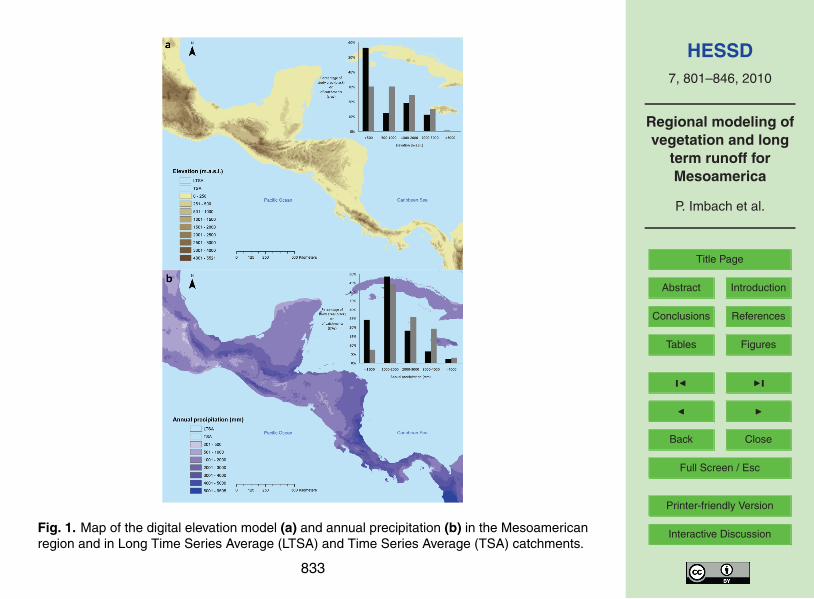
The study area spans continental land within 6.5 and 22 degrees latitude and −76.5and −99 degrees longitude. This one million square kilometer area covers South-ern Mexico in the north and the 7 Central American countries down to Panama in5
the south. This region has a highly complex biophysical environment; Hastenrath(1967) describes it as structurally rich in coast lines and plains, with high mountainsand plateaus exerting a large influence on climate. The main topographic feature isa mountain range that reaches over 4000 m. a.s.l. and runs close to the Pacific coastwith few interruptions (Fig. 1a).10
Mean annual surface temperature has small fluctuations over the year. By con-trast, precipitation is highly variable. Precipitation seasonality is determined by theInter-Tropical Convergence Zone (ITCZ), which brings convective rains. Winds comingfrom the Caribbean interact with mountains and coastlines further increasing season-ality (Nieuwolt, 1977). The result is a high variability of precipitation over short dis-15
tances, with humid windward mountains and coastal areas, and dry leeward valleys(Fig. 1b). Therefore, convective rains dominate the Atlantic watersheds and orographicrains have a higher contribution in the Pacific watersheds (Shultz, 2002; Guswa et al.,2007).
The rainy season lasts from May to October (Hastenrath, 1967). The distribution of20
precipitation is bimodal, with two maxima during June and September–October, anda distinctive relative minimum in between called the mid-summer drought (Magana etal., 1999). Runoff follows precipitation inputs because most rivers in the region are rain-fed. The longest and largest rivers are on the Atlantic side (Griesinger and Gladwell,1993).25
Vegetation of the Pacific watersheds and northern part of the Yucatan Peninsula istropical with summer rain (Schultz, 2002). The vegetation of the Atlantic watersheds istropical with year-round rain. In pristine Pacific areas, there are savanna grasslands of
805
HESSD7, 801–846, 2010
Regional modeling ofvegetation and long
term runoff forMesoamerica
P. Imbach et al.
Title Page
Abstract Introduction
Conclusions References
Tables Figures
J I
J I
Back Close
Full Screen / Esc
Printer-friendly Version
Interactive Discussion
variable tree density depending on available moisture. In the Atlantic areas, evergreenforests dominate. Anthropogenic influence has reduced natural vegetation to 58% ofthe total area. Rainfall, vegetation and high radiation, much of it being diffuse due tohigh cloud cover, leads to high annual evapotranspiration rates over 1000 mm (Shultz,2002).5
2.2 MAPSS model description
MAPSS simulates potential vegetation cover and leaf area given light and water con-straints. A monthly time step water balance is calculated based on the vegetation leafarea and stomatal conductance for canopy transpiration and soil hydrology (Neilson,1995). Interception is a function of the number of rain events and leaf area index (LAI).10
Water reaching the soil layer is divided into fast runoff and infiltration. The latter is reg-ulated by saturated and unsaturated percolation processes according to Darcy’s Law(Hillel, 1982). The soil is divided in three layers with grasses having access to waterfrom the top layer, woody vegetation from the top and intermediate layers and the deep-est layer is used for base-flow. Before percolation, transpiration by grasses and woody15
plants occurs. The ratio of actual to potential evapotranspiration (PET) increases ex-ponentially with LAI. PET is calculated using climate and an aerodynamic turbulenttransfer model (Marks, 1990). Stomatal conductance decreases with decreasing soilwater potential and with increasing PET.
The calculation of LAI involves competition for both water and light between woody20
and herbaceous vegetation. Water is provided to grasses from the first soil layerwhereas woody vegetation has access to the two top soil layers. The third and deepestsoil layer is used for base flow. The final equilibrium LAI is calculated iteratively forgrasses and woody vegetation, so that LAI consumes most of the available water ina single month of the growing period and never drops below the wilting point.25
MAPSS assumes the annual soil and aquifers water storage term (∆s) in Eq. (1) isclose to zero, which is mostly true on an annual basis or in catchments characterized
806

HESSD7, 801–846, 2010
Regional modeling ofvegetation and long
term runoff forMesoamerica
P. Imbach et al.
Title Page
Abstract Introduction
Conclusions References
Tables Figures
J I
J I
Back Close
Full Screen / Esc
Printer-friendly Version
Interactive Discussion
by a high superficial runoff to infiltration ratio:
R = P −E − I−∆s (1)
Where, R is runoff, P is precipitation, E is evapotranspiration, I is interception and ∆sis the water storage in soils and aquifers.
2.3 Model set up and input data5
We implemented MAPSS at the resolution of climate forcing data (1 km2) unless other-wise stated.
2.3.1 Precipitation
Meteorological forcing data have a strong influence on the model’s performance anduncertainty (Linde et al., 2008). This is particularly true in the topographically com-10
plex Mesoamerican region. Uncertainties in the climate input dataset could thus havea larger influence on model output in the context of our fine scale application, as com-pared to uncertainties of model parameters which are known to impact modeling hy-drology at a macro-scale (Arnell, 1999). To assess climate uncertainties, we tested 6different precipitation data sources, 4 with monthly averages of at least 30 years, and15
2 covering a 10 year average (Table 1). These precipitation datasets were:
– CRU CL 2.0: the coarsest dataset used, based on interpolation of weather sta-tions data using latitude, longitude and elevation as co-predictors (New et al.,2002)
– WorldClim: developed from weather stations data, interpolated at high resolution,20
and accounting for elevation (Hijmans et al., 2005)
– FCLIM: developed specifically for Central America by interpolation of weather sta-tions, distance to southern coastline, elevation, and precipitation data from remote
807
HESSD7, 801–846, 2010
Regional modeling ofvegetation and long
term runoff forMesoamerica
P. Imbach et al.
Title Page
Abstract Introduction
Conclusions References
Tables Figures
J I
J I
Back Close
Full Screen / Esc
Printer-friendly Version
Interactive Discussion
sensing sources by the Climate Hazard Group at the University of California inSanta Barbara3
– Wind PPT (modeling wind driven precipitation): modeled with the TRMM datasetusing wind-speed and direction as well as terrain conditions (slope, aspect andtopographic exposure) (Mulligan, 2006)5
– TRMM: developed from two remote sensing sources (a passive microwave ra-diometer and a scanning radar) to estimate rainfall (Mulligan, 2006)
– TCMF: developed by calculating a 10% increase in precipitation in the FCLIMdataset, over areas covered by cloud forests (from a map developed by Mulli-gan and Burke, 2005). As clouds go through forests in these areas, water is10
intercepted by the vegetation and adds to the total amount of water available forrunoff production. This intercepted water is not regularly captured by rain gauges.The increase in value was arbitrarily selected from a range of interception valuesranging 6 to 35% of total rainfall (Bruijnzell, 2005).
2.3.2 Sensitivity tests15
We performed three sensitivity tests. The first test uses FCLIM precipitation withMAPSS original parameters. The second test is based upon FCLIM with a calibratedMAPSS version (see section on calibration method). The third is based upon FCLIMwith a compilation of national soils maps (NS) to evaluate the effect of high resolutionsoils data (no data was available for Nicaragua and Belize).The NS soil parameters20
(texture and soil depth) compilation was made by digitizing country-wide soils mapsand analyzing their technical documentation to estimate soil texture and depths tobedrock (see Table 1 for references). Gaps in information were filled with data froma global soils map (FAO, 2003).
3data available at http://www.geog.ucsb.edu/∼diego/projects/rainfall/climatologia.html
808
HESSD7, 801–846, 2010
Regional modeling ofvegetation and long
term runoff forMesoamerica
P. Imbach et al.
Title Page
Abstract Introduction
Conclusions References
Tables Figures
J I
J I
Back Close
Full Screen / Esc
Printer-friendly Version
Interactive Discussion
2.3.3 Runoff observation at catchment scale
A new runoff dataset was created from data with different levels of temporal resolution(daily, monthly, and annual) and different series length collected from several institu-tions across the Mesoamerican region (see Table 1). The catchment boundaries ofeach runoff station were delineated using the SRTM (Shuttle Radar Topography Mis-5
sion) 90 m digital elevation model (Jarvis et al., 2008). Stream flow data in cubic me-ters per second was converted to depth values in mm by normalizing the flow with thecatchment area above the measurement point.
We selected 135 catchments (out of a total of 466 available) across the region(Fig. 1a and b) using the following criteria:10
i) Retain only catchments with an annual-runoff-precipitation ratio smaller than unity,thus excluding catchments where either precipitation interpolation or runoff dataare miscalculated,
ii) Exclude water bodies bigger than 1% of the catchment area as this could repre-sent regulated catchments,15
iii) Retain catchments with available runoff data from data series >15 years (Gertenet al., 2004) to minimize the effects of inter-annual variability (Hartshorn, 2002;Aguilar et al., 2005).
From now on, this dataset will be called the Long Time Series Average dataset (LTSA).Another runoff dataset was constructed without criteria iii), leaving 243 catchments.20
This larger dataset is called the Time Series Average dataset (TSA). TSA results arepresented separately since they are based on a larger dataset for calibration and val-idation, but could be biased by some catchments characterized by short dry or wetperiods.
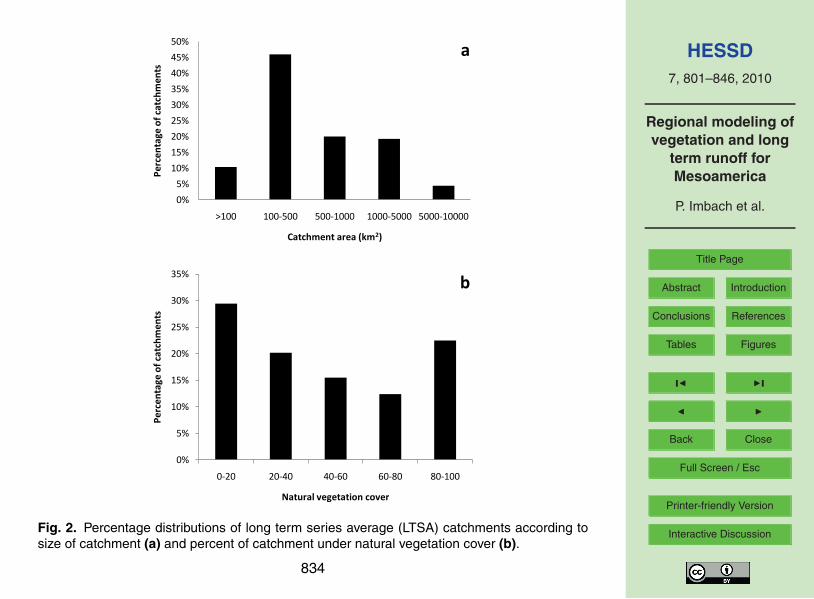
The area of each LTSA catchment ranged between less than 100 km2 to 15 378 km225
(Fig. 2a). As the difference between potential and actual vegetation may affect model
809
HESSD7, 801–846, 2010
Regional modeling ofvegetation and long
term runoff forMesoamerica
P. Imbach et al.
Title Page
Abstract Introduction
Conclusions References
Tables Figures
J I
J I
Back Close
Full Screen / Esc
Printer-friendly Version
Interactive Discussion
performance, we corroborated that these catchments represent the full range of naturalvegetation cover (Fig. 2b). Selected catchments are representative of the study areain terms of their precipitation and mean elevation (Fig. 1a and b).
On a monthly basis, the storage term ∆s of Eq. (1) can represent a substantial frac-tion of the total water budget in some catchments. These catchments are associated5
with a high coefficient of variation in their monthly R:P ratio (CV −R:P ). Thus, weperformed a monthly analysis of the model-data comparison only in catchments witha CV −R:P <0.5. This threshold was selected to minimize the effect of high ∆s vari-ability while keeping at least half of the catchments for analysis. Using this criterion,monthly model-data comparison is possible for 63 catchments in the LTSA dataset (9410
in the TSA dataset).
2.3.4 Model calibration and validation
Calibration and validation of MAPSS was performed with annual runoff data usinga split-sample test (Klemes, 1986; Xu 1999; Xu and Singh, 2004), i.e. by randomlyselecting half of the catchments for calibration and the remaining half for validation.15
This test is a common approach for splitting data into calibration and validation sets,either spatially or temporally (Motovilov et al., 1999; Wooldridge and Kalma, 2001;Donker 2001; Guo et al., 2002; Xu and Singh, 2004; Linde et al., 2008). This calibra-tion and validation method was selected due to the diversity of biophysical conditionspresent in our runoff dataset.20
We calibrated the model by manually adjusting parameters controlling transpirationand soil layer thickness until modeled runoff matched the observations. First, resultsfrom the un-calibrated MAPSS parameterization were inspected for runoff under orover prediction. Then, adjustments for reducing modeled runoff in watersheds wherethe model overestimated runoff were made, to obtain a regression curve with a slope25
close to 1 and a negative intercept. The negative intercept results from MAPSS mod-eling the potential vegetation distribution, thus having a higher evapotranspiration rateand lower runoff than observations. The actual vegetation includes pasture and crop-
810
HESSD7, 801–846, 2010
Regional modeling ofvegetation and long
term runoff forMesoamerica
P. Imbach et al.
Title Page
Abstract Introduction
Conclusions References
Tables Figures
J I
J I
Back Close
Full Screen / Esc
Printer-friendly Version
Interactive Discussion
lands which have lower transpiration rates than the potential forest vegetation (Neilson,1995; Haddeland et al., 2007; Gordon et al., 2005). Parameters selected for manualadjustment (Table 2) included:
i) Total soil layer thickness: we increased this parameter relative to its MAPSS de-fault value in our manual calibration procedure, to account for high rooting depths5
(Shenk and Jackson 2002; Ichii et al., 2007)
ii) Stomatal conductance: this parameter is also increased to reduce runoff andmatch the data (Ray Drapek and Ron Neilson, personal communication)
iii) The wilting points of trees and grassy vegetation: were decreased to match runoffdata.10
2.3.5 Model performance and efficiency
Several indices were used to compare observed against modeled annual and monthlyrunoff values for each catchment. Model performance was evaluated with the “linearregression” method (Bellocchi et al., 2009) where the R2 statistic is complemented withslope and intercepts analysis to asses over or under prediction. The water balance er-15
ror (WB) estimates the bias as a percentage in annual modeled runoff (Guo et al.,2002; Boone et al., 2004; Quintana Seguı et al., 2009) (Table 3). WB rating was basedon Moriasi et al. (2007) and Quintana Seguı et al. (2009). The LTSA dataset contains128 catchments with monthly data, for which model performances were estimated us-ing the Nash-Sutcliffe efficiency coefficient (NS, Eq. 2) (Nash and Sutcliffe, 1970) and20
Kendall’s ranked correlation coefficient (τ, Eq. 3) (Guo et al., 2002; Boone et al., 2004;Gordon et al., 2004; Quintana Seguı et al., 2009). NS and τ coefficients were ratedaccording to Moriassi et al. (2007). The NS efficiency assesses the match betweenmodeled and observed monthly values. A value of 1 indicates a perfect match whilea value of 0 means the model is as poor of a predictor as the mean of the observed25
data. Negative values indicate the mean of observed values performs better than the
811
HESSD7, 801–846, 2010
Regional modeling ofvegetation and long
term runoff forMesoamerica
P. Imbach et al.
Title Page
Abstract Introduction
Conclusions References
Tables Figures
J I
J I
Back Close
Full Screen / Esc
Printer-friendly Version
Interactive Discussion
model (Table 3). Kendall’s coefficient is calculated with ranked monthly values, to as-sess how the seasonal variation is mimicked by the model. The coefficient ranges from1, indicating a perfect agreement between the two rankings, to −1, indicating a perfectdisagreement (one ranking is the opposite of the other).
NS=1−(∑
i (Qoi −Qmi )∑i (Qoi −Qo)
)2
(2)5
Where Qoi and Qmi are the observed and modeled runoff values at time step i , respec-tively, and Qo is the average observed value.
τ =nc−nd
n(n−1)/2(3)
Where nc and nd are the number of concordant and discordant pairs and the denomi-nator is the total number of possible pairings.10
2.3.6 Performance of vegetation and LAI modeling
A crucial part of how MAPSS determines runoff is the relationship between actualtranspiration and LAI, since it not only determines water available for runoff, but thepotential vegetation type that can be supported on site. For this purpose two ob-served LAI datasets were chosen to assess model output performance (Table 1):15
EOS-Terra-MODIS (Yang et al., 2006a) and the GLOBCARBON-ESA European Re-mote Sensing (ERS-2)-ENVISAT-SPOT sensors (Plummer et al., 2006) (MODIS-LAIand GLOBCARBON-LAI, respectively).
Both LAI datasets were used to test whether the model was simulating runoff underrealistic conditions of vegetation leaf area, as this can be a relevant factor affecting20
spatial and temporal variability of runoff at large scales (Peel et al., 2004). Both LAIproducts rely on actual, not potential, land cover maps: MODIS-LAI is based on an 8-biome map derived from MODIS data (Friedl et al., 2002) and GLOBCARBON-LAI on
812
HESSD7, 801–846, 2010
Regional modeling ofvegetation and long
term runoff forMesoamerica
P. Imbach et al.
Title Page
Abstract Introduction
Conclusions References
Tables Figures
J I
J I
Back Close
Full Screen / Esc
Printer-friendly Version
Interactive Discussion
the Global Land Cover 2000 (GLC2000) map from SPOT-VEGETATION satellite (EC-JRC, 2003) (with approximate resolutions of 8 and 1 km, respectively). Comparisonswere made only in pixels where each land cover map matched the ecosystem type onthe Central America Ecosystem map (WB and CCAD, 2001). We used this map asa reference because it is based on extensive field work and high resolution imagery5
(28.5 m pixel) from Landsat TM. In contrast, within the studied region there is onlyone validation point for the GLC2000 land cover underlying the GLOBCARBON-LAIproduct (Mayaux et al., 2006), and none for the land cover map underlying the MODIS-LAI (MODIS Land Team, 2009). Additionally, both land cover maps have a much lowerresolution (1 km2) than Landsat TM. A comparison of the land cover sources used in10
the two LAI products shows best agreement on the Atlantic side of Mesoamerica andlarger differences on the Pacific side, Southern Mexico, and Southern Panama (Giri etal., 2005).
2.3.7 Uncertainty analysis
Analysis of uncertainty from model parameters was performed based on Zaehle et15
al. (2005) and using SimLab 2.2.1 software4. The uncertainty analysis is based onthe probability distribution functions (PDFs) of model parameters and their effect onmodel output. The PDFs for 61 parameters of model components controlling rainfallinterception, evapotranspiration, and soil site conditions were built based on a literaturereview of field studies. To be conservative in the uncertainty assessment, a uniform20
distribution was assumed for all parameters within the range of values found in theliterature. A 30% variance was assumed for conceptual parameters that are usedto simplify complex processes and are not measurable in experiments (Zaehle et al.,2005; see Table 1 in Supplemental material: http://www.hydrol-earth-syst-sci-discuss.net/7/801/2010/hessd-7-801-2010-supplement.pdf).25
The space of parameter PDFs was explored using a Monte Carlo-type approach,
4Available at http://simlab.jrc.ec.europa.eu/
813
HESSD7, 801–846, 2010
Regional modeling ofvegetation and long
term runoff forMesoamerica
P. Imbach et al.
Title Page
Abstract Introduction
Conclusions References
Tables Figures
J I
J I
Back Close
Full Screen / Esc
Printer-friendly Version
Interactive Discussion
the Latin-Hypercube sampling (LHS) method, to build a stratified sample of randomsets of parameter values. The LHS method has the advantage of building a strati-fied representation of all parameters with a reduced variance due to additive effectsof parameters on model output. The parameter sample consisted of 610 parametercombinations to be tested in model runs. Some runs had parameter combinations out-5
side model boundaries leading to crash-runs, leaving a total of 456 runs, well withinthe recommended amount between 3/2 (92 runs) to 10 times (610 runs) the numberof parameters (EC-JRC, 2009).
3 Results and discussion
3.1 Performance of calibrated model assessed by statistical tests10
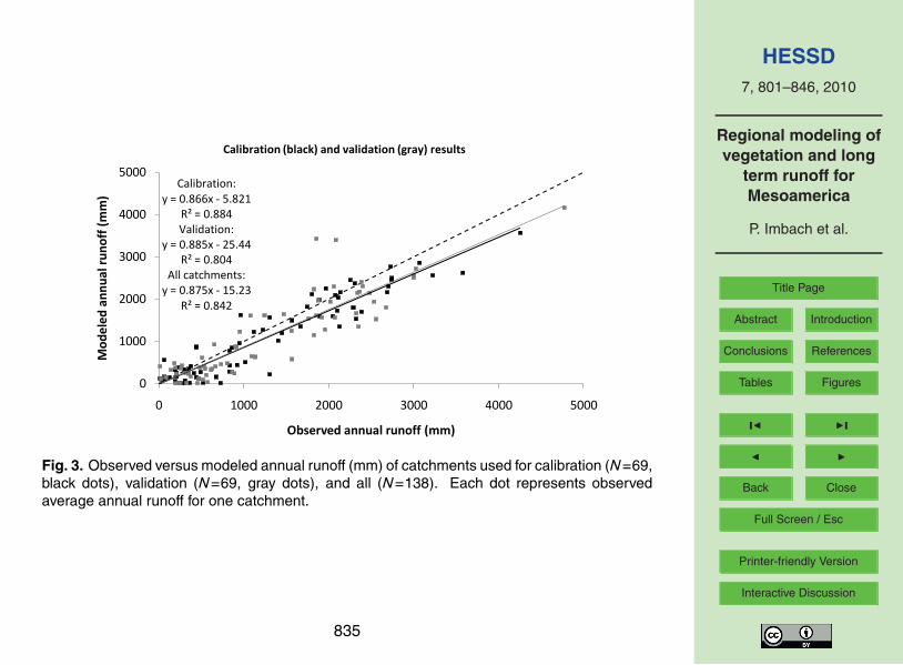
Calibration and validation of total annual runoff for LTSA catchments showed goodoverall agreement across the whole range of runoff values (1–4774 mm) and an un-derestimation of modeled runoff of around 12% (Fig. 3). In turn, calibration and vali-dation results for the TSA dataset, were also satisfactory but modeled annual runoffwas underestimated by approximately 20% (data not shown, N=251, Slope=0.81,15
Intercept=36 and R2=0.78). A similar trend was obtained when MAPSS simulatedrunoff for the United States because the model simulates potential vegetation whichhas higher evapotranspiration when compared to actual vegetation cover (Neilson,1995). Vorosmarty et al. (1989) has a similar trend when coupling water balance andwater transport models for a large scale application in South America. Results with20
un-calibrated MAPSS gave a similar slope and correlation but the intercept increasedto 145 mm.
After splitting the dataset by rainfall category we found that model performance waslower in dry areas than in wetter areas (data not shown). Similar lower performancein dry catchments was found by Gordon et al. (2004) when evaluating six terrestrial25
ecosystem models in the United States, although the runoff range they analyzed is
814
HESSD7, 801–846, 2010
Regional modeling ofvegetation and long
term runoff forMesoamerica
P. Imbach et al.
Title Page
Abstract Introduction
Conclusions References
Tables Figures
J I
J I
Back Close
Full Screen / Esc
Printer-friendly Version
Interactive Discussion
much lower than for Central America. Lower model performance is probably due tothe effect of higher uncertainties in precipitation; including rainfall frequency and localheterogeneity (rainstorms) of runoff in drier regions due to non-linearity of the runoffgeneration process (Fekete et al., 2004). It is thus possible that in dry areas, theobserved runoff is dominated by few daily events of intense precipitation that cannot5
be captured at our working monthly time steps.The monthly model performance, according to classes for NS and τ statistical crite-
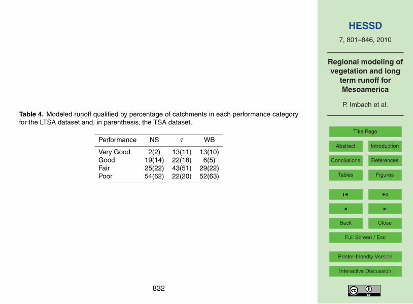
ria in Table 3, is fair or better for 46% and 78% of catchments, respectively (Table 4).Annual runoff is modeled fairly or better for 48% of the catchments (Table 4). In gen-eral, our model performance is similar to that of other studies (Artinyan et al., 2007;10
Linde et al., 2008) but slightly less than that found over France with the SIM model(Quintana Segui et al., 2009; 61% fair or better). Given the very large number of smallcatchments, complex orography, and climate uncertainties found in Mesoamerica, weconsidered our model performance satisfactory.
3.2 Performance of the model assessed by comparison with a “poor man”15
model
We compared the results of MAPSS with those of a “poor man” model where the runoffis modeled to be proportional to annual rainfall only, that is runoff=alpha×rainfall. Wetested all potential values of alpha, and the performances were always poorer thanthose of MAPSS, irrespective of the statistical criteria used. This test shows that useful20
information is contained in the MAPSS parameterization that improves the simulationof runoff in Central America, even though the model is based upon potential vegetationand runs on a monthly time step.
3.3 Modeled versus observed LAI distribution
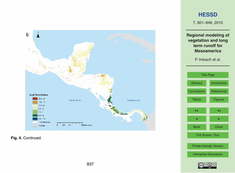
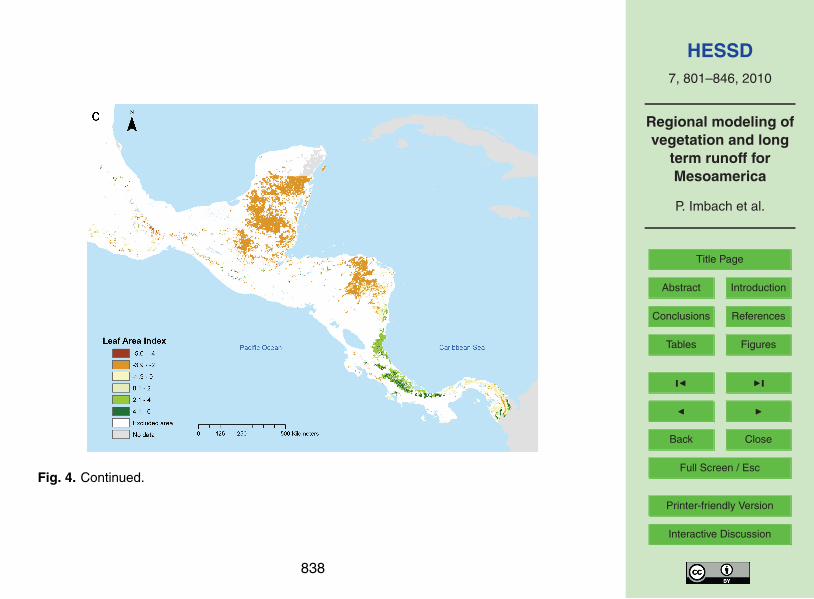
Figure 4a shows the modeled LAI by MAPSS, and the difference between modeled LAI25
and observed from MODIS and GLOBCARBON (Fig. 4b and c, respectively). Agricul-
815
HESSD7, 801–846, 2010
Regional modeling ofvegetation and long
term runoff forMesoamerica
P. Imbach et al.
Title Page
Abstract Introduction
Conclusions References
Tables Figures
J I
J I
Back Close
Full Screen / Esc
Printer-friendly Version
Interactive Discussion
tural areas and other disturbed land cover types were excluded from the LAI compari-son. Over naturally vegetated areas, the comparison was made over pixels where boththe land cover map used to generate MODIS and GLOBCARBON LAI products, andthe MAPSS vegetation, match the vegetation type on the Central American ecosys-tems map (used as the reference). Both criteria define the excluded areas category in5
Fig. 4b and c.The general feature is an under prediction of LAI in the northern part of the
Mesoamerica region and an over prediction in the South. Discrepancies appear whencomparing MODIS and GLOBCARBON LAI (Fig. 4b and c). This could be due tomisclassifications of land cover, particularly between classes with different architecture10
and foliage optics (Myneni et al., 2002; Yang et al., 2006a). Atmospheric and cloudconditions are also problematic over tropical areas, where MODIS-LAI values are cal-culated by the simpler NDVI (Normalized Difference Vegetation Index) based backupalgorithm (Myneni et al., 2002). Yang et al. (2006b), for example, found that broadleafforests (covering most of our study area) can be underestimated by as much as 3.415
LAI units. Accordingly, we found that areas with under prediction are dominated by themain algorithm and those with over prediction by the backup algorithm, except for smallareas in Southern Panama.
3.4 Residuals distribution and uncertainty analysis
There was no systematic trend in the residuals as a function of annual precipitation,20
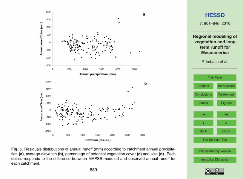
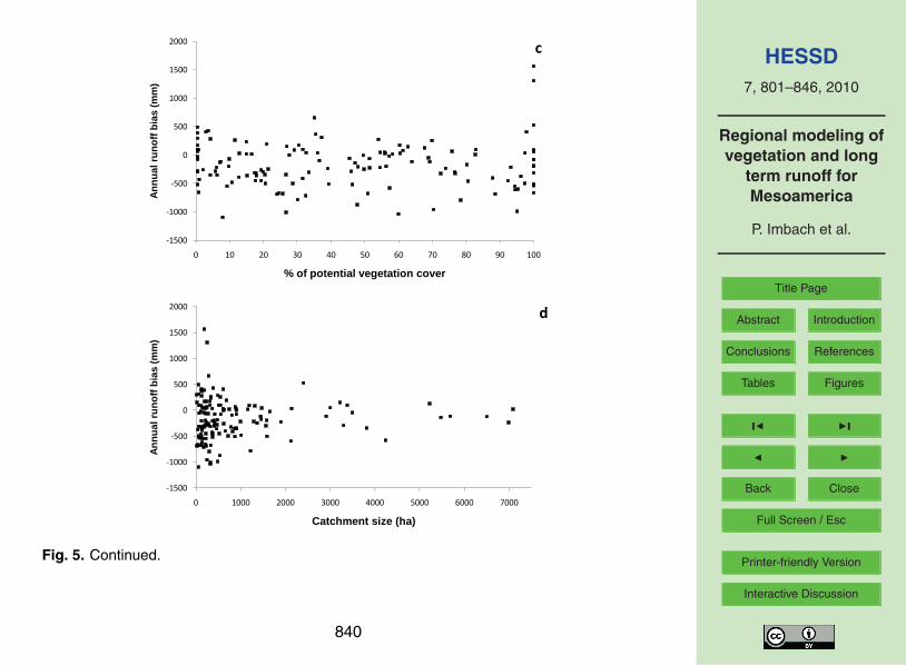
elevation or percentage of potential vegetation cover (Fig. 5a, b and c, respectively).However, larger residuals were found for small catchments (<1000 ha or 10 pixels),probably due to larger uncertainty in the delineation of each catchment.
The model systematically underestimates runoff by around 12% (Fig. 3). We couldnot detect a positive trend in the residuals with decreasing potential vegetation cover25
(Fig. 5c). Consequently, it appears that the 12% under prediction in annual runoff(Fig. 3) cannot be attributed here to the potential vegetation cover assumed by MAPSS(Neilson, 1995). We explored the possibility of missing rainfall due to cloud forest hori-
816
HESSD7, 801–846, 2010
Regional modeling ofvegetation and long
term runoff forMesoamerica
P. Imbach et al.
Title Page
Abstract Introduction
Conclusions References
Tables Figures
J I
J I
Back Close
Full Screen / Esc
Printer-friendly Version
Interactive Discussion
zontal interception (Bruijnzell, 2005; Holder, 2004; Zadroga 1981) and results showedan improvement when this type of forests are accounted for (see section on sensibilityto precipitation datasets).
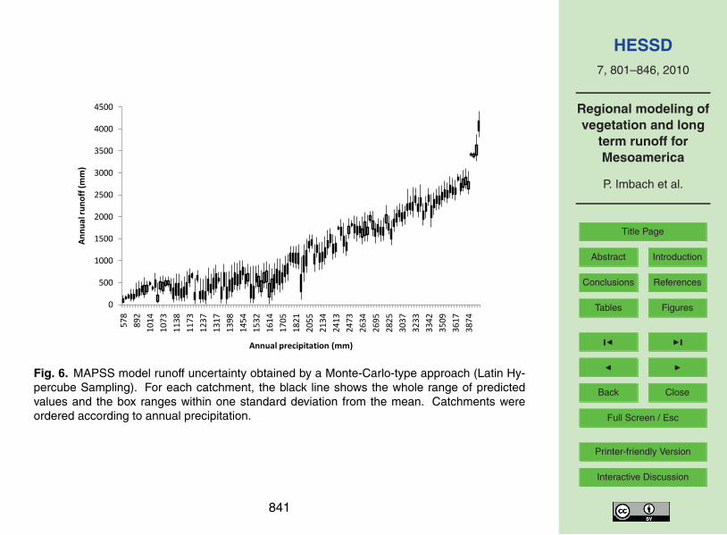
Figure 6 shows annual runoff results for each catchment from the uncertainty anal-ysis, along the annual precipitation range. For each catchment, we show the range of5
values modeled by 456 parameter combinations from the set of parameters samplesbuilt with the LHS method. The average range of modeled annual runoff values withinone standard deviation is within 36% of the total modeled range and equals 42% of theobserved annual runoff. No apparent trend in uncertainty is found along the precipita-tion range, suggesting a constant effect of parameters uncertainty along the dry to wet10
gradient.
3.5 Seasonal bias
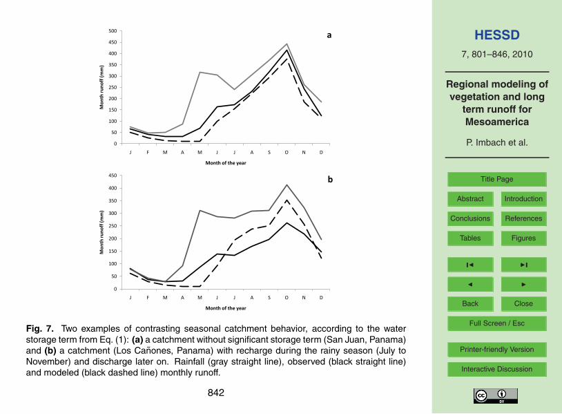
Figure 7 shows the seasonality of precipitation and runoff for two selected catchmentswith different storage terms (∆s in Eq. 1). Storage term refers to accumulation of wa-ter in unsaturated and saturated zones (aquifers). In Fig. 7a, monthly modeled runoff15
mimics the observed time course which corresponds to a situation with small ∆s. InFig. 7b, the modeled time course crosses two times the observed curve, indicatinga period of water accumulation in the basin between July and November and a periodof discharge later on. Zadroga (1981) found a similar situation in Costa Rica by ana-lyzing runoff and weather station data across 7 watersheds. Similar results were also20
found by Heyman and Kjerfve (1999) in Belize, probably due to the release of waterfrom limestone aquifers. In Nicaragua, Calderon Palma and Bentley (2007) identifiedshallow local recharge-discharge systems and a deep system that recharges in highermountains and discharges in the central and lower plains. Moreover, using isotopes inCosta Rica, Guswa et al. (2007) showed that orographic precipitation (wind driven pre-25
cipitation and fog interception) contributed to the dry season base flow and the delayedcontribution of the rainy season precipitation to dry season streamflow.
MAPSS has good performance on an annual time scale. Given that MAPSS does817
HESSD7, 801–846, 2010
Regional modeling ofvegetation and long
term runoff forMesoamerica
P. Imbach et al.
Title Page
Abstract Introduction
Conclusions References
Tables Figures
J I
J I
Back Close
Full Screen / Esc
Printer-friendly Version
Interactive Discussion
not simulate the ground water storage processes controlling the ∆s seasonal variation,it remains valid on a monthly time scale only for the selected catchments were thestorage term is not significant. MAPSS monthly performance analysis falls to 26%(fair) when considering all catchments, but increases to 54% after excluding those witha significant storage term (see model performance and efficiency section).5
3.6 Sensitivity to different precipitation input datasets
The modeled standard deviations are lower than observations (A) and correlation co-efficients similar for all precipitation forcing datasets (Fig. 8). The TRMM (G) and WindPPT (H) have good correlations (0.84 and 0.85, respectively) but the lower regressionslope among the datasets (0.66 and 0.64), probably due to extreme precipitation vari-10
ations (Fekete et al., 2004), with differences of more than 1000 mm over large areascompared to other datasets (data not shown). Wind PPT (H) has a lower regres-sion intercept (140 mm) compared to TRMM (G) (209 mm) indicating and improvementwhen accounting for winds in precipitation estimates. Accounting for cloud forests inprecipitation estimates slightly improved regression results, from FCLIM (B) to TMCF15
(F), by increasing slope (from 0.88 to 0.93) and keeping similar correlations and inter-cepts. MAPSS original parameterization (D) has good performance (Slope=0.85 andcorrelation=0.92) but the intercept is positive (133 mm). FCLIM (B) has an improvedcorrelation, smallest RMS, slope closest to 1 and standard deviation closest to thatof observed values showing the calibration improvement when compared to MAPSS20
original parameterization (D).Based on the uncertainty analysis runs, we also assessed the model sensitivity to
its parameters. We estimated the Ranked Partial Correlation Coefficient (RPCC) formodel parameters based on average annual runoff of the study area in each run ofthe uncertainty analysis (Zaehle et al., 2005). MAPSS is most sensitive to the param-25
eter that sets the ceiling for maximum stomatal conductance for all vegetation types(RPCC=0.47).
818
HESSD7, 801–846, 2010
Regional modeling ofvegetation and long
term runoff forMesoamerica
P. Imbach et al.
Title Page
Abstract Introduction
Conclusions References
Tables Figures
J I
J I
Back Close
Full Screen / Esc
Printer-friendly Version
Interactive Discussion
3.7 Regional mapping
After the model calibration and validation steps, we simulated runoff across the en-tire region and analyzed model outputs. Modeled runoff and evapotranspiration mapsshows a mean annual runoff and evapotranspiration of 552 and 1200 mm, respectively,with highest values distributed mostly in the southern part of the region and in mountain5
areas in the North Pacific side (Fig. 9a and b, respectively).We explored the water balance partitioning along the annual precipitation gradient.
Figure 10 shows the relationship between the evapotranspiration:runoff ratio (E/R) andprecipitation classes, each E/R value being an average for 100 mm annual precipita-tion classes. Below the 1500 mm annual precipitation threshold, evapotranspiration10
becomes a key component of the water balance, justifying the need of a SVAT modelsuch as MAPSS for reliable modeling of the annual water balance.
Potential vegetation types are also simulated by the model and correspond to foresttypes that appear along available humidity across the year from evergreen forests todry tropical savanna (Fig. 11). This gradient is also characterized by a gradient of LAI15
values from trees, shrubs and grasses. A detailed description of each forest type isprovided by Neilson (1995).
4 Conclusions
We calibrated and validated the SVAT hydrological model MAPSS (Neilson, 1995) forthe Mesoamerican region at 1 km resolution, after building a new database of observed20
runoff of 466 catchments. We presented a regionally calibrated version of MAPSS andoutput maps of runoff, evapotranspiration, leaf area index (LAI) and potential vegeta-tion.
Runoff prediction performed similarly to other large scale studies. A general under-estimation of 12% has been attributed by Neilson (1995) in temperate conditions to the25
fact that MAPSS simulates potential vegetation. However, our residual analyses did not
819
HESSD7, 801–846, 2010
Regional modeling ofvegetation and long
term runoff forMesoamerica
P. Imbach et al.
Title Page
Abstract Introduction
Conclusions References
Tables Figures
J I
J I
Back Close
Full Screen / Esc
Printer-friendly Version
Interactive Discussion
confirm that hypothesis. We suspect that large horizontal interception of precipitationcould play an important role in tropical mountain areas.
MAPSS simulation of monthly runoff was consistent only in catchments were thestorage term (∆s) is not significant, as this component is not simulated by the model.Availability of spatial information to estimate ∆s is a crucial limitation to improve monthly5
performance of the model.Accounting for wind and cloud forests in precipitation estimates improved results
indicating the importance of precipitation horizontal interception for runoff generationin our study area.
Modeled LAI was consistent with remotely sensed observations (MODIS and GLOB-10
CARBON) except in humid areas Mesoamerica where high levels of LAI have beenmeasured directly in the field and cloud cover is frequent. In these areas remotelysensed LAI is known to have lower quality estimates.
It is important to use a SVAT model to explicitly model actual evapotranspiration,especially in drier areas, below 1500 mm of annual precipitation, where ETR represents15
a very large fraction of the water balance.Future steps with our calibrated MAPSS version will focus on simulating the impacts
of climate change on water balance and vegetation of the Mesoamerican region.
Acknowledgements. The authors would like to express their gratitude to the Gerencia deHidrometeorologıa – Departamento de Hidrologıa from ETESA in Panama, the Centro de Ser-20
vicios Basicos and the Departamento de Hidrologıa from ICE in Costa Rica, the Gerenciade Hidrologıa – SNET from MARN in El Salvador, the Departamento de Hidrologıa from IN-SIVUMEH in Guatemala and the Departamento de Servicios Hidrologicos y Climatologicosfrom SERNA in Honduras for kindly providing runoff data that made this paper possible, toMaarten Kapelle for his useful comments and CIRAD for financial support.25
This document was produced within the framework of the project “Tropical Forests and ClimateChange Adaptation” (TroFCCA), executed by CATIE and CIFOR and funded by the EuropeanCommission under contract EuropeAid/ENV/2004-81719. The contents of this document arethe sole responsibility of the authors and can under no circumstances be regarded as reflectingthe position of the European Union.30
820
HESSD7, 801–846, 2010
Regional modeling ofvegetation and long
term runoff forMesoamerica
P. Imbach et al.
Title Page
Abstract Introduction
Conclusions References
Tables Figures
J I
J I
Back Close
Full Screen / Esc
Printer-friendly Version
Interactive Discussion
References
Abbot, B. G. H. L.: Hydrology of the isthmus of Panama, P. Natl. Acad. Sci. USA, 3, 41–47,1917.
Aguilar, E., Peterson, T. C., Obando, P. R., Frutos, R., Retana, J. A., Solera, M., Soley, J.,Garcıa, I. G., Araujo, R. M., Santos, A. R., Valle, V. E., Brunet, M., Aguilar, L., Alvarez, L.,5
Bautista, M., Castanon, C., Herrera, L., Ruano, E., Sinay, J. J., Sanchez, E., Oviedo, G. I. H.,Obed, F., Salgado, J. E., Vazquez, J. L., Baca, M., Gutierrez, M., Centella, C., Espinosa, J.,Martınez, D., Olmedo, B., Espinoza, C. E. O., Nunez, R., Haylock, M., Benavides, H., andMayorga, R.: Changes in precipitation and temperature extremes in Central America andNorthern South America, J. Geophys. Res., 110, 1961–2003, doi:10.1029/2005jd006119,10
2005.Arnell, N. W.: A simple water balance model for the simulation of streamflow over a large
geographic domain, J. Hydrol., 217, 314–335, 1999.Artinyan, E., Habets, F., Noilhan, J., Ledoux, E., Dimitrov, D., Martin, E., and Le Moigne, P.:
Modelling the water budget and the riverflows of the Maritsa basin in Bulgaria, Hydrol. Earth15
Syst. Sci., 12, 21–37, 2008,http://www.hydrol-earth-syst-sci.net/12/21/2008/.
Bellocchi, G., Rivington, M., Donatelli, M., and Matthews, K.: Validation of biophysical models:issues and methodologies, A review, Agron. Sustain. Dev., preprint, 10.1051/agro/2009001,20092009.20
Bishop, G. D., Church, M. R., Aber, J. D., Neilson, R. P., Ollinger, S. V., and Daly, C.: A compar-ison of mapped estimates of long-term runoff in the northeast United States, J. Hydrol., 206,176–190, 1998.
Boone, A., Habets, F., Noilhan, J., Clark, D., Dirmeyer, P., Fox, S., Gusev, Y., Haddeland, I.,Koster, R., Lohmann, D., Mahanama, S., Mitchell, K., Nasonova, O., Niu, G.-Y., Pitman, A.,25
Polcher, J., Shmakin, A. B., Tanaka, K., van den Hurk, B., Verant, S., Verseghy, D., Viterbo,P., and Yang, Z.-L.: The Rhone-aggregation land surface scheme intercomparison project:an overview, J. Climate, 17, 187–208, 2004.
Bruijnzell, L.: Tropical montane cloud forests: a unique hydrological case, in: Forests, Waterand People in the Humid Tropics: Past, Present and Future Hydrological Research for Inte-30
grated Land and Water Management, edited by: Bonell, M. and Bruijnzeel, L., InternationalHydrology Series, Cambridge University Press, 944 pp., 462–484, 2005.
821
HESSD7, 801–846, 2010
Regional modeling ofvegetation and long
term runoff forMesoamerica
P. Imbach et al.
Title Page
Abstract Introduction
Conclusions References
Tables Figures
J I
J I
Back Close
Full Screen / Esc
Printer-friendly Version
Interactive Discussion
Calderon Palma, H. and Bentley, L.: A regional-scale groundwater flow model for the Leon-Chinandega aquifer, Nicaragua, Hydrogeol. J., 15, 1457–1472, 2007.
Cavelier, J., Solis, D., and Jaramillo, M. A.: Fog interception in montane forests across the Cen-tral Cordillera of Panama?, J. Trop. Ecol., 12, 357–369, doi:10.1017/S026646740000955X,1996.5
Cavelier, J., Jaramillo, M., Solis, D., and de Leon, D.: Water balance and nutrient inputs in bulkprecipitation in tropical montane cloud forest in Panama, J. Hydrol., 193, 83–96, 1997.
Clark, K. L., Nadkarni, N. M., Schaefer, D., and Gholz, H. L.: Atmospheric deposition and netretention of ions by the canopy in a tropical montane forest, Monteverde, Costa Rica, J. Trop.Ecol., 14, 27–45, doi:10.1017/S0266467498000030, 1998.10
Donker, N. H. W.: A simple rainfall-runoff model based on hydrological units applied to the Tebacatchment (South-east Spain), Hydrol. Process., 15, 135–149, 2001.
EC-JRC: Global Land Cover 2000 database, European Commission, Joint Research Centre,2003.
EC-JRC: Simlab 2.2 Reference Manual, European Comission, Joint Research Center, 159,15
2009.FAO: Digital soil map of the World and derived soil properties, Rev. 1st edn., 2003.Fekete, B. M., Vorosmarty, C. J., and Grabs, W.: High-resolution fields of global runoff com-
bining observed river discharge and simulated water balances, Global Biogeochem. Cy., 16,1042, doi:10.1029/1999gb001254, 2002.20
Friedl, M. A., McIver, D. K., Hodges, J. C. F., Zhang, X. Y., Muchoney, D., Strahler, A. H.,Woodcock, C. E., Gopal, S., Schneider, A., Cooper, A., Baccini, A., Gao, F., and Schaaf,C.: Global land cover mapping from MODIS: algorithms and early results, Remote Sens.Environ., 83, 287–302, 2002.
Genereux, D. P. and Jordan, M.: Interbasin groundwater flow and groundwater interaction with25
surface water in a lowland rainforest, Costa Rica: a review, J. Hydrol., 320, 385–399, 2006.Gerten, D., Schaphoff, S., Haberlandt, U., Lucht, W., and Sitch, S.: Terrestrial vegetation and
water balance-hydrological evaluation of a dynamic global vegetation model, J. Hydrol., 286,249–270, 2004.
Giri, C., Zhu, Z., and Reed, B.: A comparative analysis of the global land cover 2000 and30
MODIS land cover data sets, Remote Sens. Environ., 94, 123–132, 2005.Gordon, W. S., Famiglietti, J. S., Fowler, N. L., Kittel, T. G. F., and Hibbard, K. A.: Validation of
simulated runoff from six terrestrial ecosystem models: results from VEMAP, Ecol. Appl., 14,
822
HESSD7, 801–846, 2010
Regional modeling ofvegetation and long
term runoff forMesoamerica
P. Imbach et al.
Title Page
Abstract Introduction
Conclusions References
Tables Figures
J I
J I
Back Close
Full Screen / Esc
Printer-friendly Version
Interactive Discussion
527–545, doi:10.1890/02-5287, 2004.Gordon, L. J., Steffen, W., Jonsson, B. F., Folke, C., Falkenmark, M., and Johannessen, A.:
Human modification of global water vapor flows from the land surface, P. Natl. Acad. Sci.USA, 102, 7612–7617, doi:10.1073/pnas.0500208102, 2005.
Griesinger, B. and Gladwell, J.: Hydrology and water resources in tropical Latin America and5
the Caribbean, in: Hydrology and Water Management in the Humid Tropics: HydrologicalResearch Issues and Strategies for Water Management, edited by: Bonell, M., Hufschmidt,M., and Gladwell, J., Cambridge University Press, 84–97, 1993.
Guo, S., Wang, J., Xiong, L., Ying, A., and Li, D.: A macro-scale and semi-distributed monthlywater balance model to predict climate change impacts in China, J. Hydrol., 268, 1–15,10
2002.Guswa, A. J., Rhodes, A. L., and Newell, S. E.: Importance of orographic precipitation to the
water resources of Monteverde, Costa Rica, Adv. Water Resour., 30, 2098–2112, 2007.Haddeland, I., Skaugen, T., and Lettenmaier, D. P.: Hydrologic effects of land and water man-
agement in North America and Asia: 1700-1992, Hydrol. Earth Syst. Sci., 11, 1035–1045,15
2007,http://www.hydrol-earth-syst-sci.net/11/1035/2007/.
Hartshorn, G.: Biogeografıa de los bosques tropicales, in: Ecologıa y Conservacion deBosques Neotropicales, edited by: Guariguata, M. and Kattan, G., Ediciones LUR, SanJose, Costa Rica, 692, 2002.20
Hastenrath, S.: Rainfall distribution and regime in Central America, Theor. Appl. Climatol., 15,201–241, 1967.
Heyman, W. D. and Kjerfve, B.: Hydrological and oceanographic considerations for integratedcoastal zone management in Southern Belize, Environ. Manage., 24, 229–245, 1999.
Hijmans, R. J., Cameron, S. E., Parra, J. L., Jones, P. G., and Jarvis, A.: Very high resolution25
interpolated climate surfaces for global land areas, Int. J. Climatol., 25, 1965–1978, 2005.Hillel, D.: Introduction to Soil Physics, Academic Press, 364 pp., 1982.Holder, C. D.: Fog precipitation in the Sierra de las Minas biosphere reserve, Guatemala,
Hydrol. Process., 17, 2001–2010, 2003.Holder, C. D.: Rainfall interception and fog precipitation in a tropical montane cloud forest of30
Guatemala, Forest. Ecol. Manag., 190, 373–384, 2004.Ichii, K., Hashimoto, H., White, M. A., Potter, C., Hutyra, L. R., Huete, A. R., Myneni, R. B., and
Nemani, R. R.: Constraining rooting depths in tropical rainforests using satellite data and
823
HESSD7, 801–846, 2010
Regional modeling ofvegetation and long
term runoff forMesoamerica
P. Imbach et al.
Title Page
Abstract Introduction
Conclusions References
Tables Figures
J I
J I
Back Close
Full Screen / Esc
Printer-friendly Version
Interactive Discussion
ecosystem modeling for accurate simulation of gross primary production seasonality, Glob.Change Biol., 13, 67–77, 2007.
IDIAP: Zonificacion de suelos de Panama por niveles de nutrientes, Instituto de InvestigacionAgropecuaria de Panama, Ciudad de Panama, Panama, 2006.
INEGI: Carta Edafologica, Instituto Nacional de Estadıstica y Geografıa, Mexico, 1984.5
Jarvis, A., Reuter, H., Nelson, A., and Guevara, E.: Hole-filled seamless SRTM data, 4th edn.,International Center for Tropical Agriculture (CIAT), 2008.
Kaimowitz, D.: Useful myths and intractable truths: the politics of the link between forests andwater in Central America, in: Forests, Water and People in the Humid Tropics: Past, Presentand Future Hydrological Research for Integrated Land and Water Management, edited by:10
Bonell, M. and Bruijnzeel, L., International Hydrology Series, Cambridge University Press,925 pp., 89–98, 2005.
Klemes, V.: Operational testing of hydrological simulation models, Hydrolog. Sci. J., 31, 13–24,1986.
te Linde, A. H., Aerts, J. C. J. H., Hurkmans, R. T. W. L., and Eberle, M.: Comparing model15
performance of two rainfall-runoff models in the Rhine basin using different atmosphericforcing data sets, Hydrol. Earth Syst. Sci., 12, 943–957, 2008,http://www.hydrol-earth-syst-sci.net/12/943/2008/.
Magana, V., Amador, J. A., and Medina, S.: The midsummer drought over Mexico and CentralAmerica, J. Climate, 12, 1577–1588, 1999.20
Marks, D.: The sensitivity of potential evapotranspiration to climate change over the continentalUnited States, US Environmental Protection Agency, Corvallis, Oregon, USA, IV-1–IV-31,1990.
Mayaux, P., Eva, H., Gallego, J., Strahler, A. H., Herold, M., Agrawal, S., Naumov, S., DeMiranda, E. E., Di Bella, C. M., Ordoyne, C., Kopin, Y., and Roy, P. S.: Validation of the global25
land cover 2000 map, IEEE T. Geosci. Remote., 44, 1728–1739, 2006.MODIS Land Team: Validation of Consistent-Year V003 Land Cover Product: http://
www-modis.bu.edu/landcover/userguidelc/consistent.htm, 2009.Moriasi, D. N., Arnold, J. G., Van Liew, M. W., Bingner, R. L., Harmel, R. D., and Veith, T. L.:
Model evaluation guidelines for systematic quantification of accuracy in watershed simula-30
tions, T. ASABE, 50, 885–900, 2007.Motovilov, Y. G., Gottschalk, L., Engeland, K., and Rodhe, A.: Validation of a distributed hydro-
logical model against spatial observations, Agr. Forest Meteorol., 98–99, 257–277, 1999.
824
HESSD7, 801–846, 2010
Regional modeling ofvegetation and long
term runoff forMesoamerica
P. Imbach et al.
Title Page
Abstract Introduction
Conclusions References
Tables Figures
J I
J I
Back Close
Full Screen / Esc
Printer-friendly Version
Interactive Discussion
Mulligan, M. and Burke, S. M.: Global cloud forests and environmental change in a hydrologicalcontext, http://www.ambiotek.com/cloudforests/, 2005.
Mulligan, M.: Global griddded 1 km TRMM rainfall climatology and derivatives, Version 1.0 ed.,2006.
Myneni, R. B., Hoffman, S., Knyazikhin, Y., Privette, J. L., Glassy, J., Tian, Y., Wang, Y., Song,5
X., Zhang, Y., Smith, G. R., Lotsch, A., Friedl, M., Morisette, J. T., Votava, P., Nemani, R. R.,and Running, S. W.: Global products of vegetation leaf area and fraction absorbed PAR fromyear one of MODIS data, Remote Sens. Environ., 83, 214–231, 2002.
Nash, J. E. and Sutcliffe, J. V.: River flow forecasting through conceptual models, Part I: A dis-cussion of principles, J. Hydrol., 10, 282–290, 1970.10
Neilson, R. P.: A Model for Predicting Continental-Scale Vegetation Distribution and WaterBalance, Ecol. Appl., 5, 362–385, doi:10.2307/1942028, 1995.
New, M., Lister, D., Hulme, M., and Makin, I.: A high-resolution data set of surface climate overglobal land areas, Clim. Res., 21, 1–25, doi:10.3354/cr021001, 2002.
Niedzialek, J. and Ogden, F.: Runoff Production in the Upper Rio Chagres Watershed, Panama,15
in: The Rio Chagres, Panama. A Multidisciplinary Profile of a Tropical Watershed edited by:Singh, V. P. and Harmon, R. S., Water Science and Technology Library, Springer Nether-lands, 149–168, 2005.
Nieuwolt, S.: Tropical Climatology: An Introduction to the Climates of the Low Latitudes, JohnWiley, New York, USA, 207 pp., 1977.20
Nijssen, B., Donnell, G. M., Lettenmaier, D. P., Lohmann, D., and Wood, E. F.: Predicting thedischarge of global rivers, J. Climate, 14, 3307–3323, 2001.
Peel, M. C., McMahon, T. A., and Finlayson, B. L.: Continental differences in the variability ofannual runoff-update and reassessment, J. Hydrol., 295, 185–197, 2004.
Perez, S., Ramırez, E., Alvarado, A., and Knox, E.: Manual descriptivo del mapa de asocia-25
ciones de sub-grupos de suelos de Costa Rica (escala 1:200 000), Oficina de PlanificacionSectorial Agropecuaria, San Jose, Costa Rica, 236 pp., 1979.
Plummer, S., Arino, O., Simon, M., and Steffen, W.: Establishing an earth observation productservice for the terrestrial carbon community: the globcarbon initiative, Mitigation and Adap-tation Strategies for Global Change, 11, 97–111, 2006.30
Quintana Seguı, P., Martin, E., Habets, F., and Noilhan, J.: Improvement, calibration and vali-dation of a distributed hydrological model over France, Hydrol. Earth Syst. Sci., 13, 163–181,2009,
825
HESSD7, 801–846, 2010
Regional modeling ofvegetation and long
term runoff forMesoamerica
P. Imbach et al.
Title Page
Abstract Introduction
Conclusions References
Tables Figures
J I
J I
Back Close
Full Screen / Esc
Printer-friendly Version
Interactive Discussion
http://www.hydrol-earth-syst-sci.net/13/163/2009/.Schenk, H. J. and Jackson, R. B.: The global biogeography of roots, Ecol. Monogr., 72, 311–
328, doi:10.1890/0012-9615(2002)072[0311:TGBOR]2.0.CO;2, 2002.Schultz, J.: The Ecozones of the world, in: The Ecological Divisions of the Geosphere, 2nd
edn., Springer-Verlag, Netherlands, 252 pp., 2002.5
Siebert, S. and Doll, P.: A Digital Global Map of Irrigated Areas – An Update for Latin Americaand Europe, Center for Environmental Systems Research, KasselA0102, 2001.
Simmons, C., Tarano, T., and Pinto, J.: Clasificacion de reconocimiento de los suelos de laRepublica de Guatemala, Instituto Agropecuario Nacional, Guatemala, 1959.
Simmons, C.: Los suelos de Honduras, Informe al Gobierno de Honduras, FAO, Roma, Italia,10
88, 1969.Thattai, D., Kjerfve, B., and Heyman, W. D.: Hydrometeorology and variability of water dis-
charge and sediment load in the inner Gulf of Honduras, Western Caribbean, J. Hydromete-orol, 4, 985–995, 2003.
Vorosmarty, C. J., Moore, B. III, Grace, A. L., Gildea, M. P., Melillo, J. M., Peterson,15
B. J., Rastetter, E. B., and Steudler, P. A.: Continental scale models of water bal-ance and fluvial transport: an application to South America, Global Biogeochem. Cy., 3,doi:10.1029/GB003i003p00241, 1989.
WB and CCAD: Ecosistemas de Mesoamerica, World Bank (WB), Comision Centroamericanade Ambiente y Desarrollo (CCAD), 2001.20
Wolf, A., Yoffe, S., and Giordano, M.: International Waters: identifying basins at risk, WaterPolicy, 5, 29–60, 2003.
Wooldridge, S. A. and Kalma, J. D.: Regional-scale hydrological modelling using multiple-parameter landscape zones and a quasi-distributed water balance model, Hydrol. Earth Syst.Sci., 5, 59–74, 2001,25
http://www.hydrol-earth-syst-sci.net/5/59/2001/.Xu, C.-Y.: Operational testing of a water balance model for predicting climate change impacts,
Agr. Forest Meteorol., 98–99, 295–304, 1999.Xu, C. Y., and Singh, V. P.: Review on regional water resources assessment models under
stationary and changing climate, Water Resour. Manag., 18, 591–612, 2004.30
Yang, W., Huang, D., Tan, B., Stroeve, J. C., Shabanov, N. V., Knyazikhin, Y., Nemani, R. R.,and Myneni, R. B.: Analysis of leaf area index and fraction of PAR absorbed by vegetationproducts from the terra MODIS sensor: 2000–2005, IEEE T. Geosci. Remote, 44, 1829–
826
HESSD7, 801–846, 2010
Regional modeling ofvegetation and long
term runoff forMesoamerica
P. Imbach et al.
Title Page
Abstract Introduction
Conclusions References
Tables Figures
J I
J I
Back Close
Full Screen / Esc
Printer-friendly Version
Interactive Discussion
1842, 2006a.Yang, W., Tan, B., Huang, D., Rautiainen, M., Shabanov, N. V., Wang, Y., Privette, J. L., Huemm-
rich, K. F., Fensholt, R., Sandholt, I., Weiss, M., Ahl, D. E., Gower, S. T., Nemani, R. R.,Knyazikhin, Y., and Myneni, R. B.: MODIS leaf area index products: from validation to algo-rithm improvement, IEEE T. Geosci. Remote, 44, 1885–1898, 2006b.5
Zadroga, F.: The hydrological importance of a montane cloud forest area in Costa Rica, in:Tropical Agricultural Hydrology, Watershed Management and Land Use, edited by: Lal, R.and Russel, W., Wiley, New York, USA, 59–73, 1981.
Zaehle, S., Sitch, S., Smith, B., and Hatterman, F.: Effects of parameter uncertainties onthe modeling of terrestrial biosphere dynamics, Global Biogeochem. Cy., 19, GB3020,10
doi:10.1029/2004gb002395, 2005.
827
HESSD7, 801–846, 2010
Regional modeling ofvegetation and long
term runoff forMesoamerica
P. Imbach et al.
Title Page
Abstract Introduction
Conclusions References
Tables Figures
J I
J I
Back Close
Full Screen / Esc
Printer-friendly Version
Interactive Discussion
Table 1. Data sources for model input, calibration and validation.
Name Variable Resolution/Time period Source
SOILS AND TOPOGRAPHYNS Soils Percentage of clay, 1:200 000 (Costa Rica) Perez et al. (1979)
sand and depth 1:250 000 (Guatemala, Mexico) Simmons et al. (1959)to bedrock 1:500 000 (Honduras) Simmons (1969)
Not reported for Panama IDIAP (2006)INEGI (1984)
World Soils Percentage of clay, 1:5 000 000 FAO (2003)sand and depthto bedrock
SRTM Elevation 30 arc s Jarvis et al. (2008)
CLIMATECRU CL2.0 Temperature precipitation, 10 min/1961–1990 New et al. (2002)
wind speedWorldClim Temperature, precipitationb 30 arc s/1950–2000 Hijmans et al. (2005)FCLIM Precipitationa,b 5 km/1960–2000 University of Santa Monicac
Wind PPT Precipitationa,b 1 km/1997–2006 Mulligan (2006)TRMM 2b31-Based Rainfall Precipitationa,b 1 km/1997–2006 Mulligan (2006)Climatology Version 1.0
LEAF AREA INDEXGLOBCARBON-LAI Leaf area index 1 km/1998–2007 average http://geofront.vgt.vito.beMODIS-LAI Leaf area index 1 km/Mar 2000–May Boston Universityd
2009 average
VEGETATION COVERGlobal biomes Vegetation type 8 km/2006 Boston Universityd
Global land cover 2000 Vegetation type 1 km/2000 EC-JRC (2003)Cloud forests % of cloud forest 1 km Mulligan and Burke (2005)
828
HESSD7, 801–846, 2010
Regional modeling ofvegetation and long
term runoff forMesoamerica
P. Imbach et al.
Title Page
Abstract Introduction
Conclusions References
Tables Figures
J I
J I
Back Close
Full Screen / Esc
Printer-friendly Version
Interactive Discussion
Table 1. Continued.
RUNOFFCountry No. of
catch-ments
Timesteps(smaller)
Serieslength
Average Data provider
Panama 84 Monthly Yes All years Empresa de TransmisionElectrica S.A. (ETESA)
Costa Rica 128 Daily Yes Year Instituto Costarricense deElectricidad (ICE)
Nicaragua 33 Monthly Yes Year Ministerio del Ambientey los Recursos Naturales(MARENA)
Honduras 48 Monthly Yes Year Secretarıa de RecursosNaturales y Ambiente
El Salvador 22 Monthly Yes All years Ministerio del Ambiente yRecursos Naturales
Guatemala 6/31/73 Monthly/Monthly/Year
Yes/No/No
Year/All Years/All years
Instituto Nacional deSismologıa, Vulcanologıa,Meteorologıa e Hidrologıa
Mexico (12 south-ern most states)
603 Daily Yes Year Instituto Mexicano de Tec-nologıa del Agua
a Worldclim temperature was used hereb CRU wind speed was used herec http://www.geog.ucsb.edu/∼diego/projects/rainfall/climatologia.htmld http://cybele.bu.edu/modismisr/index.html
829
HESSD7, 801–846, 2010
Regional modeling ofvegetation and long
term runoff forMesoamerica
P. Imbach et al.
Title Page
Abstract Introduction
Conclusions References
Tables Figures
J I
J I
Back Close
Full Screen / Esc
Printer-friendly Version
Interactive Discussion
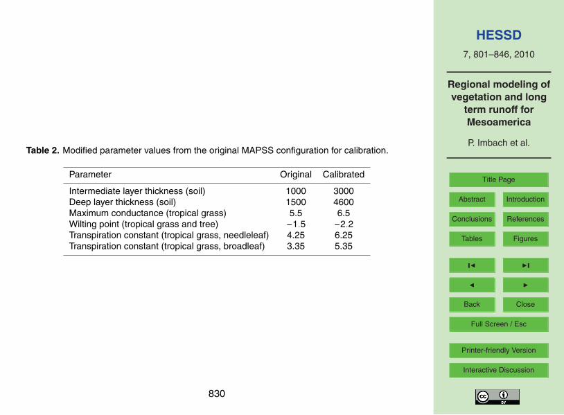
Table 2. Modified parameter values from the original MAPSS configuration for calibration.
Parameter Original Calibrated
Intermediate layer thickness (soil) 1000 3000Deep layer thickness (soil) 1500 4600Maximum conductance (tropical grass) 5.5 6.5Wilting point (tropical grass and tree) −1.5 −2.2Transpiration constant (tropical grass, needleleaf) 4.25 6.25Transpiration constant (tropical grass, broadleaf) 3.35 5.35
830
HESSD7, 801–846, 2010
Regional modeling ofvegetation and long
term runoff forMesoamerica
P. Imbach et al.
Title Page
Abstract Introduction
Conclusions References
Tables Figures
J I
J I
Back Close
Full Screen / Esc
Printer-friendly Version
Interactive Discussion
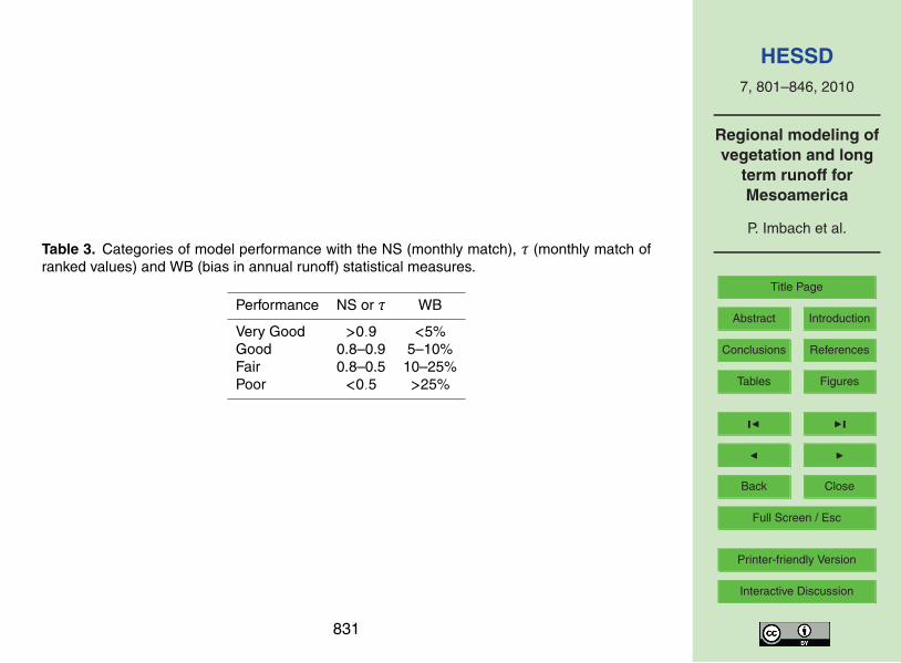
Table 3. Categories of model performance with the NS (monthly match), τ (monthly match ofranked values) and WB (bias in annual runoff) statistical measures.
Performance NS or τ WB
Very Good >0.9 <5%Good 0.8–0.9 5–10%Fair 0.8–0.5 10–25%Poor <0.5 >25%
831
HESSD7, 801–846, 2010
Regional modeling ofvegetation and long
term runoff forMesoamerica
P. Imbach et al.
Title Page
Abstract Introduction
Conclusions References
Tables Figures
J I
J I
Back Close
Full Screen / Esc
Printer-friendly Version
Interactive Discussion
Table 4. Modeled runoff qualified by percentage of catchments in each performance categoryfor the LTSA dataset and, in parenthesis, the TSA dataset.
Performance NS τ WB
Very Good 2(2) 13(11) 13(10)Good 19(14) 22(18) 6(5)Fair 25(22) 43(51) 29(22)Poor 54(62) 22(20) 52(63)
832
HESSD7, 801–846, 2010
Regional modeling ofvegetation and long
term runoff forMesoamerica
P. Imbach et al.
Title Page
Abstract Introduction
Conclusions References
Tables Figures
J I
J I
Back Close
Full Screen / Esc
Printer-friendly Version
Interactive DiscussionFig. 1. Map of the digital elevation model (a) and annual precipitation (b) in the Mesoamericanregion and in Long Time Series Average (LTSA) and Time Series Average (TSA) catchments.
833
HESSD7, 801–846, 2010
Regional modeling ofvegetation and long
term runoff forMesoamerica
P. Imbach et al.
Title Page
Abstract Introduction
Conclusions References
Tables Figures
J I
J I
Back Close
Full Screen / Esc
Printer-friendly Version
Interactive Discussion
33
781
782
Figure 2. Percentage distributions of long term series average (LTSA) catchments 783
according to size of catchment (a) and percent of catchment under natural vegetation 784
cover (b). 785
786
0%
5%
10%
15%
20%
25%
30%
35%
40%
45%
50%
>100 100-500 500-1000 1000-5000 5000-10000
Pe
rce
nta
ge o
f ca
tch
men
ts
Catchment area (km2)
a
0%
5%
10%
15%
20%
25%
30%
35%
0-20 20-40 40-60 60-80 80-100
Pe
rce
nta
ge o
f ca
tch
men
ts
Natural vegetation cover
b
Fig. 2. Percentage distributions of long term series average (LTSA) catchments according tosize of catchment (a) and percent of catchment under natural vegetation cover (b).
834
HESSD7, 801–846, 2010
Regional modeling ofvegetation and long
term runoff forMesoamerica
P. Imbach et al.
Title Page
Abstract Introduction
Conclusions References
Tables Figures
J I
J I
Back Close
Full Screen / Esc
Printer-friendly Version
Interactive Discussion
34
787
788
Figure 3. Observed versus modeled annual runoff (mm) of catchments used for 789
calibration (N=69, black dots), validation (N=69, gray dots), and all (N=138). Each dot 790
represents observed average annual runoff for one catchment. 791
792
Calibration: y = 0.866x - 5.821
R² = 0.884Validation:
y = 0.885x - 25.44R² = 0.804
All catchments:y = 0.875x - 15.23
R² = 0.842
0
1000
2000
3000
4000
5000
0 1000 2000 3000 4000 5000
Mo
del
ed a
nn
ual
ru
no
ff (
mm
)
Observed annual runoff (mm)
Calibration (black) and validation (gray) results
Fig. 3. Observed versus modeled annual runoff (mm) of catchments used for calibration (N=69,black dots), validation (N=69, gray dots), and all (N=138). Each dot represents observedaverage annual runoff for one catchment.
835

HESSD7, 801–846, 2010
Regional modeling ofvegetation and long
term runoff forMesoamerica
P. Imbach et al.
Title Page
Abstract Introduction
Conclusions References
Tables Figures
J I
J I
Back Close
Full Screen / Esc
Printer-friendly Version
Interactive Discussion
Fig. 4. Validation of MAPSS LAI output. (a) LAI modeled by MAPSS, (b) and (c) difference be-tween LAI simulated by MAPSS and the MODIS and GLOBCARBON global satellite products,respectively. White areas were excluded due to land cover characteristics criteria. MAPSS LAIrepresents an average LAI based on 30 to 50 year climate averages, while MODIS is the LAIaverage between 2000 and 2009 and GLOBCARBON between 1998 and 2007.
836
HESSD7, 801–846, 2010
Regional modeling ofvegetation and long
term runoff forMesoamerica
P. Imbach et al.
Title Page
Abstract Introduction
Conclusions References
Tables Figures
J I
J I
Back Close
Full Screen / Esc
Printer-friendly Version
Interactive Discussion
Fig. 4. Continued.
837
HESSD7, 801–846, 2010
Regional modeling ofvegetation and long
term runoff forMesoamerica
P. Imbach et al.
Title Page
Abstract Introduction
Conclusions References
Tables Figures
J I
J I
Back Close
Full Screen / Esc
Printer-friendly Version
Interactive Discussion
Fig. 4. Continued.
838
HESSD7, 801–846, 2010
Regional modeling ofvegetation and long
term runoff forMesoamerica
P. Imbach et al.
Title Page
Abstract Introduction
Conclusions References
Tables Figures
J I
J I
Back Close
Full Screen / Esc
Printer-friendly Version
Interactive Discussion
38
805
806
807
808
809
-1500
-1000
-500
0
500
1000
1500
2000
0 1000 2000 3000 4000 5000
An
nu
al
run
off
bia
s (
mm
)
Annual precipitation (mm)
a
-1500
-1000
-500
0
500
1000
1500
2000
0 500 1000 1500 2000 2500 3000
An
nu
al r
un
off
bia
s (m
m)
Elevation (m.a.s.l.)
b
Fig. 5. Residuals distributions of annual runoff (mm) according to catchment annual precipita-tion (a), average elevation (b), percentage of potential vegetation cover (c) and size (d). Eachdot corresponds to the difference between MAPSS-modeled and observed annual runoff foreach catchment.
839
HESSD7, 801–846, 2010
Regional modeling ofvegetation and long
term runoff forMesoamerica
P. Imbach et al.
Title Page
Abstract Introduction
Conclusions References
Tables Figures
J I
J I
Back Close
Full Screen / Esc
Printer-friendly Version
Interactive Discussion
39
810
811
Figure 5. Residuals distributions of annual runoff (mm) according to catchment 812
annual precipitation (a), average elevation (b), percentage of potential vegetation 813
cover (c) and size (d). Each dot corresponds to the difference between MAPSS-814
modeled and observed annual runoff for each catchment. 815
816
-1500
-1000
-500
0
500
1000
1500
2000
0 10 20 30 40 50 60 70 80 90 100
An
nu
al
run
off
bia
s (
mm
)
% of potential vegetation cover
c
-1500
-1000
-500
0
500
1000
1500
2000
0 1000 2000 3000 4000 5000 6000 7000
An
nu
al
run
off
bia
s (
mm
)
Catchment size (ha)
d
Fig. 5. Continued.
840
HESSD7, 801–846, 2010
Regional modeling ofvegetation and long
term runoff forMesoamerica
P. Imbach et al.
Title Page
Abstract Introduction
Conclusions References
Tables Figures
J I
J I
Back Close
Full Screen / Esc
Printer-friendly Version
Interactive Discussion
40
817
818
819
Figure 6. MAPSS model runoff uncertainty obtained by a Monte-Carlo-type approach 820
(Latin Hypercube Sampling). For each catchment, the black line shows the whole 821
range of predicted values and the box ranges withini one standard deviation from the 822
mean. Catchments were ordered according to annual precipitation. 823
824
0
500
1000
1500
2000
2500
3000
3500
4000
4500
578
892
1014
1073
1138
1173
1237
1317
1398
1454
1532
1614
1705
1821
2055
2134
2413
2473
2634
2695
2825
3037
3233
3342
3509
3617
3874
An
nu
al r
un
off
(m
m)
Annual precipitation (mm)
Fig. 6. MAPSS model runoff uncertainty obtained by a Monte-Carlo-type approach (Latin Hy-percube Sampling). For each catchment, the black line shows the whole range of predictedvalues and the box ranges within one standard deviation from the mean. Catchments wereordered according to annual precipitation.
841
HESSD7, 801–846, 2010
Regional modeling ofvegetation and long
term runoff forMesoamerica
P. Imbach et al.
Title Page
Abstract Introduction
Conclusions References
Tables Figures
J I
J I
Back Close
Full Screen / Esc
Printer-friendly Version
Interactive Discussion
41
825
826 Figure 7. Two examples of contrasting seasonal catchment behavior, according to 827
the water storage term from Equation 1: (a) a catchment without significant storage 828
term (San Juan, Panama) and (b) a catchment (Los Cañones, Panama) with 829
recharge during the rainy season (July to November) and discharge later on. Rainfall 830
(gray straight line), observed (black straight line) and modeled (black dashed line) 831
monthly runoff. 832
833
0
50
100
150
200
250
300
350
400
450
500
J F M A M J J A S O N D
Mo
nth
ru
no
ff (
mm
)
Month of the year
a
0
50
100
150
200
250
300
350
400
450
J F M A M J J A S O N D
Mo
nth
ru
no
ff (
mm
)
Month of the year
b
Fig. 7. Two examples of contrasting seasonal catchment behavior, according to the waterstorage term from Eq. (1): (a) a catchment without significant storage term (San Juan, Panama)and (b) a catchment (Los Canones, Panama) with recharge during the rainy season (July toNovember) and discharge later on. Rainfall (gray straight line), observed (black straight line)and modeled (black dashed line) monthly runoff.
842
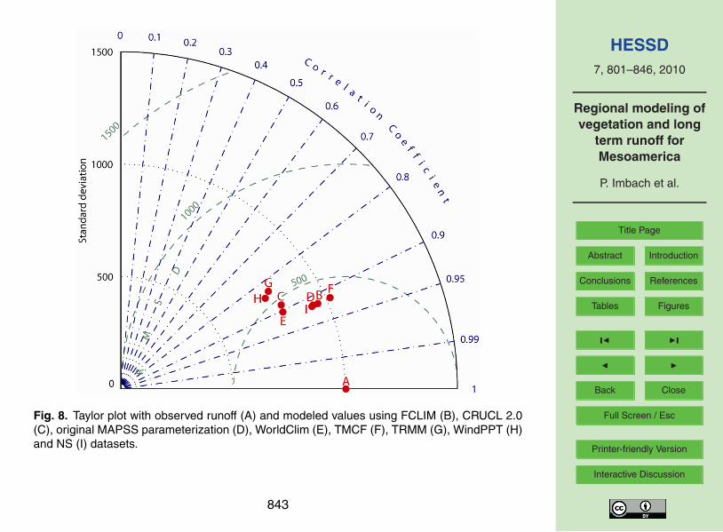
HESSD7, 801–846, 2010
Regional modeling ofvegetation and long
term runoff forMesoamerica
P. Imbach et al.
Title Page
Abstract Introduction
Conclusions References
Tables Figures
J I
J I
Back Close
Full Screen / Esc
Printer-friendly Version
Interactive Discussion
42
834
Figure 8. Taylor plot with observed runoff (A) and modeled values using FCLIM (B), 835
CRUCL 2.0 (C), original MAPSS parameterization (D), WorldClim (E), TMCF (F), 836
TRMM (G), WindPPT (H) and NS (I) datasets. 837
838
Fig. 8. Taylor plot with observed runoff (A) and modeled values using FCLIM (B), CRUCL 2.0(C), original MAPSS parameterization (D), WorldClim (E), TMCF (F), TRMM (G), WindPPT (H)and NS (I) datasets.
843
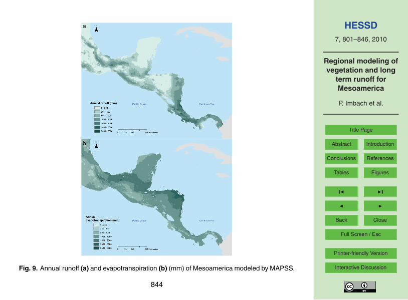
HESSD7, 801–846, 2010
Regional modeling ofvegetation and long
term runoff forMesoamerica
P. Imbach et al.
Title Page
Abstract Introduction
Conclusions References
Tables Figures
J I
J I
Back Close
Full Screen / Esc
Printer-friendly Version
Interactive DiscussionFig. 9. Annual runoff (a) and evapotranspiration (b) (mm) of Mesoamerica modeled by MAPSS.
844
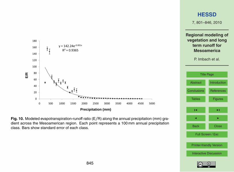
HESSD7, 801–846, 2010
Regional modeling ofvegetation and long
term runoff forMesoamerica
P. Imbach et al.
Title Page
Abstract Introduction
Conclusions References
Tables Figures
J I
J I
Back Close
Full Screen / Esc
Printer-friendly Version
Interactive Discussion
45
844
Figure 10. Modeled evapotranspiration-runoff ratio (E/R) along the annual 845
precipitation (mm) gradient across the Mesoamerican region. Each point represents a 846
100 mm annual precipitation class. Bars show standard error of each class. 847
848
y = 142.24e-0.001x
R² = 0.9365
0
20
40
60
80
100
120
140
160
180
0 500 1000 1500 2000 2500 3000 3500 4000 4500 5000
E/R
Precipitation (mm)
Fig. 10. Modeled evapotranspiration-runoff ratio (E/R) along the annual precipitation (mm) gra-dient across the Mesoamerican region. Each point represents a 100 mm annual precipitationclass. Bars show standard error of each class.
845
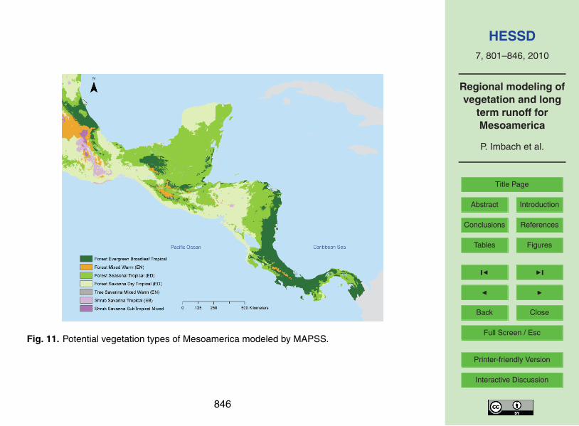
HESSD7, 801–846, 2010
Regional modeling ofvegetation and long
term runoff forMesoamerica
P. Imbach et al.
Title Page
Abstract Introduction
Conclusions References
Tables Figures
J I
J I
Back Close
Full Screen / Esc
Printer-friendly Version
Interactive Discussion
Fig. 11. Potential vegetation types of Mesoamerica modeled by MAPSS.
846


![[Vegetation and Remote Sensing] Vegetation](https://img.pdfslide.us/doc/110x75/577cdfd71a28ab9e78b21a32/vegetation-and-remote-sensing-vegetation.jpg)