Embed Size (px)
Citation preview

Regional Kinematics of the Heart:
Investigation with Marker Tracking and with
Phase Contrast Magnetic Resonance Imaging
Katarina Kindberg LITH-IMT/BMS20-EX--03/354--SE
2003-12-12
UpphovsrättDetta dokument hålls tillgängligt på Internet – eller dess framtida ersättare –under 25 år från publiceringsdatum under förutsättning att inga extraordinäraomständigheter uppstår.
Tillgång till dokumentet innebär tillstånd för var och en att läsa, ladda ner,skriva ut enstaka kopior för enskilt bruk och att använda det oförändrat för icke-kommersiell forskning och för undervisning. Överföring av upphovsrätten viden senare tidpunkt kan inte upphäva detta tillstånd. All annan användning avdokumentet kräver upphovsmannens medgivande. För att garantera äktheten,säkerheten och tillgängligheten finns lösningar av teknisk och administrativ art.
Upphovsmannens ideella rätt innefattar rätt att bli nämnd som upphovsman iden omfattning som god sed kräver vid användning av dokumentet på ovan be-skrivna sätt samt skydd mot att dokumentet ändras eller presenteras i sådan formeller i sådant sammanhang som är kränkande för upphovsmannens litterära ellerkonstnärliga anseende eller egenart.
För ytterligare information om Linköping University Electronic Press se för-lagets hemsida http://www.ep.liu.se/
CopyrightThe publishers will keep this document online on the Internet – or its possiblereplacement – for a period of 25 years from the date of publication barringexceptional circumstances.
The online availability of the document implies a permanent permission foranyone to read, to download, to print out single copies for your own use and touse it unchanged for any non-commercial research and educational purpose.Subsequent transfers of copyright cannot revoke this permission. All other usesof the document are conditional on the consent of the copyright owner. Thepublisher has taken technical and administrative measures to assure authenticity,security and accessibility.
According to intellectual property law the author has the right to be men-tioned when his/her work is accessed as described above and to be protectedagainst infringement.
For additional information about the Linköping University Electronic Pressand its procedures for publication and for assurance of document integrity,please refer to its www home page: http://www.ep.liu.se/
© Katarina Kindberg
Linköpings tekniska högskola Institutionen för medicinsk teknik
ISRN:LITH-IMT/BMS20-EX--03/354--SE Datum: 2003-12-12
Svensk titel
Engelsk titel
Regional Kinematics of the Heart: Investigation with Marker Tracking and with Phase Contrast Magnetic Resonance Imaging
Författare
Katarina Kindberg
URL: http://www.ep.liu.se/exjobb/imt/bms20/2003/354/ Uppdragsgivare: IMT, CMIV
Rapporttyp: Examensarbete
Rapportspråk: Engelska
Sammanfattning (högst 150 ord). Abstract (150 words) The pumping performance of the heart is affected by the mechanical properties of the
muscle fibre part of the cardiac wall, the myocardium. The myocardium has a complex structure, where muscle fibres have different orientations at different locations, and during the cardiac cycle, the myocardium undergoes large elastic deformations. Hence, myocardial strain pattern is complex. In this thesis work, a computation method for myocardial strain and a detailed map of myocardial transmural strain during the cardiac cycle are found by the use of surgically implanted metallic markers and beads. The strain is characterized in a local cardiac coordinate system. Thereafter, non-invasive phase contrast magnetic resonance imaging (PC-MRI) is used to compare strain at different myocardial regions. The difference in resolution between marker data and PC-MRI data is elucidated and some of the problems associated with the low resolution of PC-MRI are given.
Nyckelord (högst 8) Keyword (8 words) Strain, tensor, markers, PC-MRI, myocardium Bibliotekets anteckningar:

Regional Kinematics of the Heart:
Investigation with Marker Tracking and with
Phase Contrast Magnetic Resonance Imaging
Katarina Kindberg
2003-12-12
LiU-IMT-EX-354
Examiner and Supervisor: Matts Karlsson

Abstract The pumping performance of the heart is affected by the mechanical properties of the muscle fibre part of the cardiac wall, the myocardium. The myocardium has a complex structure, where muscle fibres have different orientations at different locations, and during the cardiac cycle, the myocardium undergoes large elastic deformations. Hence, myocardial strain pattern is complex. In this thesis work, a computation method for myocardial strain and a detailed map of myocardial transmural strain during the cardiac cycle are found by the use of surgically implanted metallic markers and beads. The strain is characterized in a local cardiac coordinate system. Thereafter, non-invasive phase contrast magnetic resonance imaging (PC-MRI) is used to compare strain at different myocardial regions. The difference in resolution between marker data and PC-MRI data is elucidated and some of the problems associated with the low resolution of PC-MRI are given.

Acknowledgements There are several people who support me and make me happy and thereby help me do a good job. My supervisor and examiner Matts Karlsson has, by his contacts at Stanford University, made research with the marker technique possible, and I am grateful for that. I would also like to thank him for his large and infectious enthusiasm and for his generosity with time. Also, I would like to send thanks to my colleagues at IMV (Institution of Medicine and Care) at Linköping University Hospital, for creating a nice atmosphere with a large sense of humour. Finally, thanks to my family and, most of all, to my husband Martin, for all your love and for encouraging me when needed. Katarina Kindberg Linköping, December 2003

Glossary Anterior Nearer to the front of the body
Apex of the Heart The tip of the heart, see figure 2.1
Apical Directed to the apex
Basal Directed to the base
Base of the Ventricle The opposite part of the ventricle compared to apex
Canine Derived from dog
Cardiac Has to do with the heart
Diastole The filling phase of the heart
Equator of the Ventricle The middle of the ventricle, between apex and base
Inferior Away from the head or toward the lower part of a structure
Lateral Farther from the midline of a structure
Myocardium The muscle fibre part of the cardiac wall
Ovine Derived from sheep
PC-MRI Phase contrast magnetic resonance imaging
Posterior Nearer to the back of the body
Sarcomere A contractile unit in a striated muscle fibre
Septal At the septum, i.e. at the wall dividing the two ventricles of the heart
Superior Toward the head or upper part of a structure
Systole The ejection phase of the heart
Transmural Through an anatomical wall
Contents
Contents 1 INTRODUCTION .............................................................................................................................................. 1
1.1 AIMS OF THIS PROJECT ................................................................................................................................ 1 1.2 CLINICAL APPLICATION............................................................................................................................... 1
2 CARDIAC ANATOMY AND PHYSIOLOGY................................................................................................ 3 2.1 ANATOMY OF THE HEART............................................................................................................................ 3 2.2 PHYSIOLOGY OF THE HEART........................................................................................................................ 4
3 DATA ACQUISITION ...................................................................................................................................... 7 3.1 INVASIVE METHOD: MARKER TRACKING .................................................................................................... 7 3.2 NON-INVASIVE METHOD: MAGNETIC RESONANCE IMAGING (MRI) ........................................................... 8
3.2.1 Phase Contrast Magnetic Resonance Imaging (PC-MRI)...................................................................... 9 3.2.2 Alternative methods................................................................................................................................ 9
3.3 RESOLUTION.............................................................................................................................................. 10 3.4 PLANES OF IMAGING.................................................................................................................................. 10
4 MECHANICS OF THE HEART .................................................................................................................... 11 4.1 THE TENSOR .............................................................................................................................................. 11
4.1.1 Symmetric-Antisymmetric Decomposition............................................................................................ 11 4.1.2 Eigenvector - Eigenvalue Decomposition ............................................................................................ 12
4.2 STRAIN ...................................................................................................................................................... 13 4.2.1 The Determinant of the Strain Tensor.................................................................................................. 15 4.2.2 Strain Components of the Cardiac Wall............................................................................................... 16
5 METHOD.......................................................................................................................................................... 17 5.1 CARDIAC COORDINATE SYSTEM................................................................................................................ 17 5.2 STRAIN COMPUTATION .............................................................................................................................. 17
5.2.1 Bead Strain........................................................................................................................................... 18 5.2.2 PC-MRI Strain ..................................................................................................................................... 19 5.2.3 Comparison of Bead and PC-MRI Strain............................................................................................. 21
6 RESULTS.......................................................................................................................................................... 23 6.1 BEAD STRAIN ............................................................................................................................................ 23 6.2 PC-MRI STRAIN ........................................................................................................................................ 25
6.2.1 Strain Tensor Determinants ................................................................................................................. 25 6.2.2 Regional Strain..................................................................................................................................... 26
6.3 COMPARISON OF BEAD AND PC-MRI STRAINS.......................................................................................... 29 7 DISCUSSION.................................................................................................................................................... 31
7.1 BEAD STRAIN ............................................................................................................................................ 31 7.2 PC-MRI STRAIN ........................................................................................................................................ 32 7.3 COMPARISON OF BEAD AND PC-MRI STRAIN ........................................................................................... 33 7.4 ALTERNATIVE STRAIN COMPUTATION METHODS...................................................................................... 34
8 FUTURE WORK.............................................................................................................................................. 35 8.1 SEVERAL NORMAL SUBJECTS .................................................................................................................... 35 8.2 STRAIN IN FIBRE- AND SHEET ORIENTATIONS ........................................................................................... 35
8.2.1 Higher Resolution of PC-MRI.............................................................................................................. 36 8.3 ALTERNATIVE FINITE ELEMENTS............................................................................................................... 36
9 APPENDIX A: OVERVIEW OF CARDIAC STRAIN EXAMINATION.................................................. 37 10 APPENDIX B: CARDIAC COORDINATE SPECIFICS............................................................................. 39

Contents
10.1 MARKER AND BEAD ARRAY...................................................................................................................... 39 10.2 PC-MRI TRACKED PARTICLE ARRAY........................................................................................................ 39
11 APPENDIX C: MEAN AND STANDARD DEVIATION STRAIN............................................................. 41 12 REFERENCES ................................................................................................................................................. 43
Introduction 1
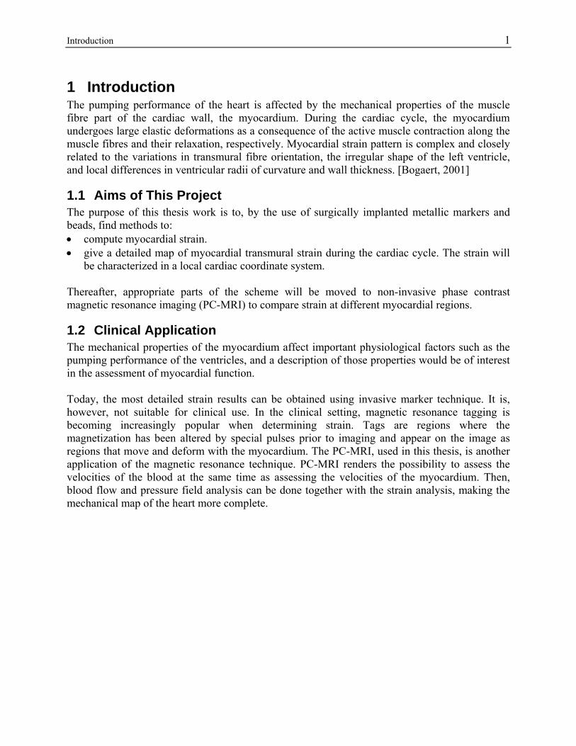
1 Introduction The pumping performance of the heart is affected by the mechanical properties of the muscle fibre part of the cardiac wall, the myocardium. During the cardiac cycle, the myocardium undergoes large elastic deformations as a consequence of the active muscle contraction along the muscle fibres and their relaxation, respectively. Myocardial strain pattern is complex and closely related to the variations in transmural fibre orientation, the irregular shape of the left ventricle, and local differences in ventricular radii of curvature and wall thickness. [Bogaert, 2001]
1.1 Aims of This Project The purpose of this thesis work is to, by the use of surgically implanted metallic markers and beads, find methods to: • compute myocardial strain. • give a detailed map of myocardial transmural strain during the cardiac cycle. The strain will
be characterized in a local cardiac coordinate system. Thereafter, appropriate parts of the scheme will be moved to non-invasive phase contrast magnetic resonance imaging (PC-MRI) to compare strain at different myocardial regions.
1.2 Clinical Application The mechanical properties of the myocardium affect important physiological factors such as the pumping performance of the ventricles, and a description of those properties would be of interest in the assessment of myocardial function. Today, the most detailed strain results can be obtained using invasive marker technique. It is, however, not suitable for clinical use. In the clinical setting, magnetic resonance tagging is becoming increasingly popular when determining strain. Tags are regions where the magnetization has been altered by special pulses prior to imaging and appear on the image as regions that move and deform with the myocardium. The PC-MRI, used in this thesis, is another application of the magnetic resonance technique. PC-MRI renders the possibility to assess the velocities of the blood at the same time as assessing the velocities of the myocardium. Then, blood flow and pressure field analysis can be done together with the strain analysis, making the mechanical map of the heart more complete.

2 Introduction
Cardiac Anatomy and Physiology 3
2 Cardiac Anatomy and Physiology This chapter gives a background to this survey by exploring the anatomy and physiology of the heart.
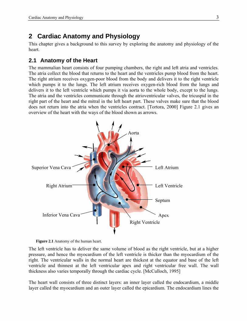
2.1 Anatomy of the Heart The mammalian heart consists of four pumping chambers, the right and left atria and ventricles. The atria collect the blood that returns to the heart and the ventricles pump blood from the heart. The right atrium receives oxygen-poor blood from the body and delivers it to the right ventricle which pumps it to the lungs. The left atrium receives oxygen-rich blood from the lungs and delivers it to the left ventricle which pumps it via aorta to the whole body, except to the lungs. The atria and the ventricles communicate through the atrioventricular valves, the tricuspid in the right part of the heart and the mitral in the left heart part. These valves make sure that the blood does not return into the atria when the ventricles contract. [Tortora, 2000] Figure 2.1 gives an overview of the heart with the ways of the blood shown as arrows.
Apex Right Ventricle
Left Ventricle
Left Atrium
Septum
Aorta
Inferior Vena Cava
Superior Vena Cava
Right Atrium
Figure 2.1 Anatomy of the human heart.
The left ventricle has to deliver the same volume of blood as the right ventricle, but at a higher pressure, and hence the myocardium of the left ventricle is thicker than the myocardium of the right. The ventricular walls in the normal heart are thickest at the equator and base of the left ventricle and thinnest at the left ventricular apex and right ventricular free wall. The wall thickness also varies temporally through the cardiac cycle. [McCulloch, 1995] The heart wall consists of three distinct layers: an inner layer called the endocardium, a middle layer called the myocardium and an outer layer called the epicardium. The endocardium lines the
4 Cardiac Anatomy and Physiology
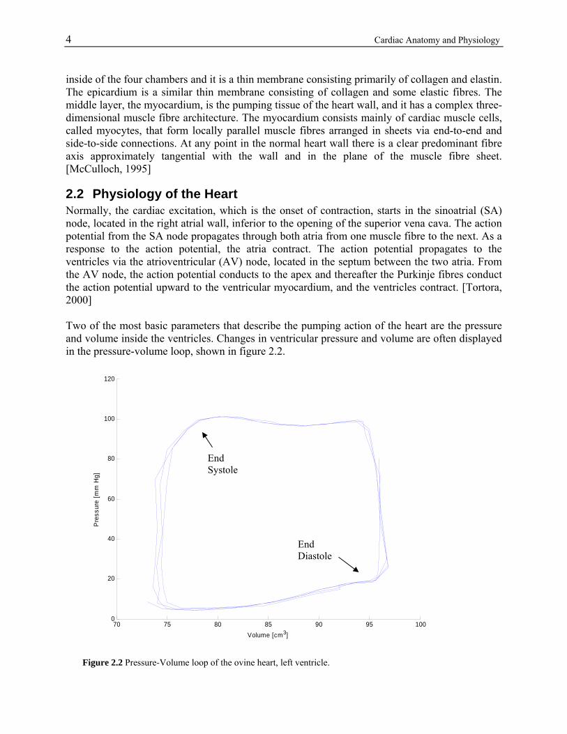
Figure 2.2 Pressure-Volume loop of the ovine heart, left ventricle.
inside of the four chambers and it is a thin membrane consisting primarily of collagen and elastin. The epicardium is a similar thin membrane consisting of collagen and some elastic fibres. The middle layer, the myocardium, is the pumping tissue of the heart wall, and it has a complex three-dimensional muscle fibre architecture. The myocardium consists mainly of cardiac muscle cells, called myocytes, that form locally parallel muscle fibres arranged in sheets via end-to-end and side-to-side connections. At any point in the normal heart wall there is a clear predominant fibre axis approximately tangential with the wall and in the plane of the muscle fibre sheet. [McCulloch, 1995]
2.2 Physiology of the Heart Normally, the cardiac excitation, which is the onset of contraction, starts in the sinoatrial (SA) node, located in the right atrial wall, inferior to the opening of the superior vena cava. The action potential from the SA node propagates through both atria from one muscle fibre to the next. As a response to the action potential, the atria contract. The action potential propagates to the ventricles via the atrioventricular (AV) node, located in the septum between the two atria. From the AV node, the action potential conducts to the apex and thereafter the Purkinje fibres conduct the action potential upward to the ventricular myocardium, and the ventricles contract. [Tortora, 2000] Two of the most basic parameters that describe the pumping action of the heart are the pressure and volume inside the ventricles. Changes in ventricular pressure and volume are often displayed in the pressure-volume loop, shown in figure 2.2.
70 75 80 85 90 95 1000
20
40
60
80
100
120
Volume [cm3]
Pre
ssur
e [m
m H
g]
Pressure-Volume loop
End Systole
End Diastole
Cardiac Anatomy and Physiology 5
Time changes in volume and pressure can be seen by following the curve counterclockwise. The isovolumic phases (isovolumic contraction and relaxation, respectively) of the cardiac cycle can be recognized as the vertical segments of the loop, whereas the lower limb represents ventricular filling and the upper limb the ejection phase. The difference on the horizontal axis between the isovolumic segments is the stroke volume. The area inside the loop represents the stroke work W performed by the myocardium on the ejected blood.
∫=ESV
EDV
dvtPW )( (eq. 2.1)
In the equation above, EDV = End Diastolic Volume and ESV = End Systolic Volume. Plotting this stroke work against a suitable measure of preload gives a ventricular function curve that illustrates an important intrinsic mechanical property of the heart as a pump, namely the Frank-Starling Law of the Heart, which states that the work of the heart increases with ventricular filling. [Humphrey, 2002]

6 Cardiac Anatomy and Physiology
Data Acquisition 7
3 Data Acquisition When studying the cardiac wall during the cardiac cycle, the data can be acquired by different techniques. Below is an overview of some of the most common data acquisition methods for obtaining four dimensional (three spatial dimensions + time) strain given, namely the marker technique and different applications of magnetic resonance imaging.
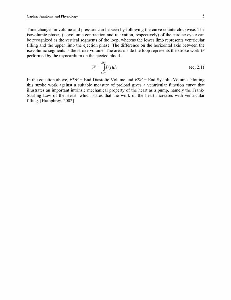
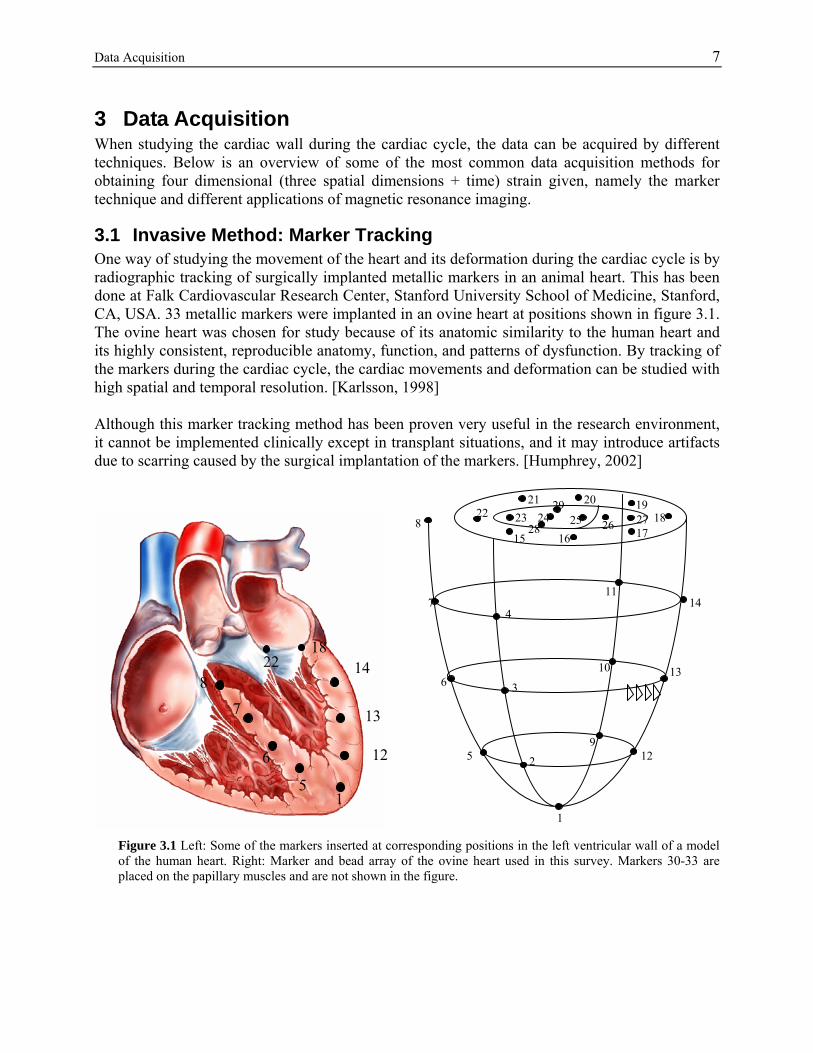
3.1 Invasive Method: Marker Tracking One way of studying the movement of the heart and its deformation during the cardiac cycle is by radiographic tracking of surgically implanted metallic markers in an animal heart. This has been done at Falk Cardiovascular Research Center, Stanford University School of Medicine, Stanford, CA, USA. 33 metallic markers were implanted in an ovine heart at positions shown in figure 3.1. The ovine heart was chosen for study because of its anatomic similarity to the human heart and its highly consistent, reproducible anatomy, function, and patterns of dysfunction. By tracking of the markers during the cardiac cycle, the cardiac movements and deformation can be studied with high spatial and temporal resolution. [Karlsson, 1998] Although this marker tracking method has been proven very useful in the research environment, it cannot be implemented clinically except in transplant situations, and it may introduce artifacts due to scarring caused by the surgical implantation of the markers. [Humphrey, 2002]
22 18
15 16 17
19 20 21
27 25 26 23 24 29
28
13
11
10
9 12
7
6
5
4
2
3
1
8
14
22 18
7
6
5 1
14 8
13
12
Figure 3.1 Left: Some of the markers inserted at corresponding positions in the left ventricular wall of a model of the human heart. Right: Marker and bead array of the ovine heart used in this survey. Markers 30-33 are placed on the papillary muscles and are not shown in the figure.
8 Data Acquisition 3.2 Non-Invasive Method: Magnetic Resonance Imaging (MRI) Non-invasiveness is of interest when studying normal humans in research and in the clinical situation. This can be performed by magnetic resonance. A quick background to the theory of magnetic resonance technique is given here, but a more extensive explanation can be found in [Wigström, 1996, Wigström 2003]. The idea is to use the inherent property of nuclear spin in the hydrogen atom (1H) in the water molecule. When creating an external magnetic field B0, the microscopic magnetic moment vector, µ, of the spin starts to precess around the axis of the external magnetic field B0 (z-axis), with a frequency, ω0, called the Larmor frequency.
0Bγω −=0 (eq. 3.1)
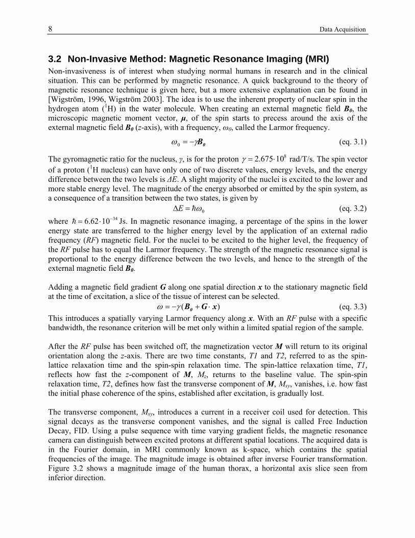
The gyromagnetic ratio for the nucleus, γ, is for the proton 810675.2 ⋅=γ rad/T/s. The spin vector of a proton (1H nucleus) can have only one of two discrete values, energy levels, and the energy difference between the two levels is ∆E. A slight majority of the nuclei is excited to the lower and more stable energy level. The magnitude of the energy absorbed or emitted by the spin system, as a consequence of a transition between the two states, is given by 0ωh=∆E (eq. 3.2) where 341062.6 −⋅=h Js. In magnetic resonance imaging, a percentage of the spins in the lower energy state are transferred to the higher energy level by the application of an external radio frequency (RF) magnetic field. For the nuclei to be excited to the higher level, the frequency of the RF pulse has to equal the Larmor frequency. The strength of the magnetic resonance signal is proportional to the energy difference between the two levels, and hence to the strength of the external magnetic field B0. Adding a magnetic field gradient G along one spatial direction x to the stationary magnetic field at the time of excitation, a slice of the tissue of interest can be selected. )( xGB0 ⋅+−= γω (eq. 3.3) This introduces a spatially varying Larmor frequency along x. With an RF pulse with a specific bandwidth, the resonance criterion will be met only within a limited spatial region of the sample. After the RF pulse has been switched off, the magnetization vector M will return to its original orientation along the z-axis. There are two time constants, T1 and T2, referred to as the spin-lattice relaxation time and the spin-spin relaxation time. The spin-lattice relaxation time, T1, reflects how fast the z-component of M, Mz, returns to the baseline value. The spin-spin relaxation time, T2, defines how fast the transverse component of M, Mxy, vanishes, i.e. how fast the initial phase coherence of the spins, established after excitation, is gradually lost. The transverse component, Mxy, introduces a current in a receiver coil used for detection. This signal decays as the transverse component vanishes, and the signal is called Free Induction Decay, FID. Using a pulse sequence with time varying gradient fields, the magnetic resonance camera can distinguish between excited protons at different spatial locations. The acquired data is in the Fourier domain, in MRI commonly known as k-space, which contains the spatial frequencies of the image. The magnitude image is obtained after inverse Fourier transformation. Figure 3.2 shows a magnitude image of the human thorax, a horizontal axis slice seen from inferior direction.
Data Acquisition 9
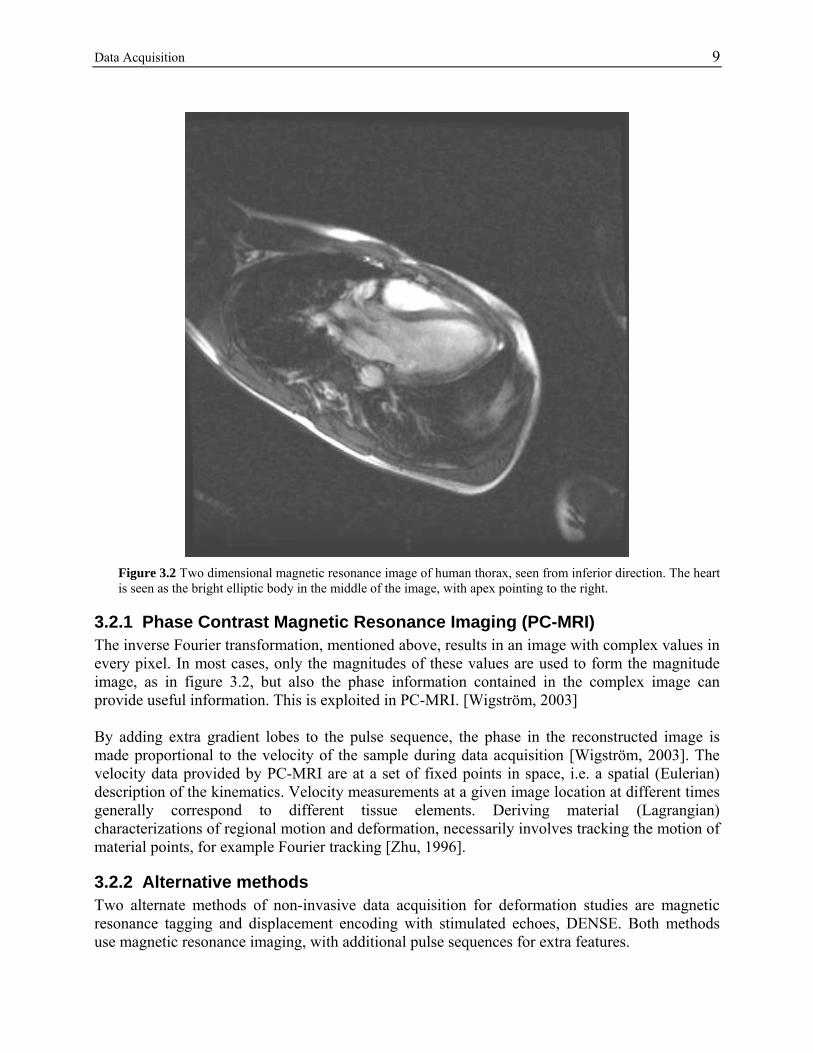
Figure 3.2 Two dimensional magnetic resonance image of human thorax, seen from inferior direction. The heart is seen as the bright elliptic body in the middle of the image, with apex pointing to the right.
3.2.1 Phase Contrast Magnetic Resonance Imaging (PC-MRI) The inverse Fourier transformation, mentioned above, results in an image with complex values in every pixel. In most cases, only the magnitudes of these values are used to form the magnitude image, as in figure 3.2, but also the phase information contained in the complex image can provide useful information. This is exploited in PC-MRI. [Wigström, 2003] By adding extra gradient lobes to the pulse sequence, the phase in the reconstructed image is made proportional to the velocity of the sample during data acquisition [Wigström, 2003]. The velocity data provided by PC-MRI are at a set of fixed points in space, i.e. a spatial (Eulerian) description of the kinematics. Velocity measurements at a given image location at different times generally correspond to different tissue elements. Deriving material (Lagrangian) characterizations of regional motion and deformation, necessarily involves tracking the motion of material points, for example Fourier tracking [Zhu, 1996].
3.2.2 Alternative methods Two alternate methods of non-invasive data acquisition for deformation studies are magnetic resonance tagging and displacement encoding with stimulated echoes, DENSE. Both methods use magnetic resonance imaging, with additional pulse sequences for extra features.
10 Data Acquisition Magnetic Resonance Tagging A relatively frequent method of non-invasive investigation of the cardiac movements and deformation is the using of magnetic resonance tagging. Tags are regions where the magnetization has been altered by special MR pulses prior to imaging and hence produce a signal difference compared to non-tagged regions. Tags appear on the MRI images as dark lines that move and deform with the myocardium on which they were inscribed [Bogaert, 2001]. While easy to visualize and implement, tagging methods suffer from low spatial resolution and transmural variations in motion are therefore difficult to measure. [Aletras, 1999]
Displacement Encoding with Stimulated Echoes (DENSE) Compared to magnetic resonance tagging, displacement encoding with stimulated echoes, DENSE, provide high spatial density of displacement measurements. Compared to PC-MRI, the same spatial resolution can be obtained, but if the tissue velocities are low, less magnetic gradient strength has to be used. In DENSE, the phase of each pixel is modulated according to its position rather than to its velocity. Using a pulse echo, the displacement of a spin can be assessed, and hence myocardial displacement mapping is made possible. With DENSE, high contrast between myocardium and blood can be acquired. [Aletras, 1999]
3.3 Resolution An organ or a body can be described at different scales. At the macro scale, the body or the organ is described as a whole entity with, for example, values of pressure, volume or a description of a twist of the body/organ. An example at macro scale is the pressure-volume loop shown in figure 2.2 and the stroke work in equation 2.1. At the meso scale, hybrid models of very detailed organs are created. One such model could be the transmural strain map acquired with bead data in this survey. At the micro scale, the model of the organ is at the level of sarcomere length. An example at the micro scale could be a detailed description of strain in fibre and cross-fibre directions. The strain results acquired using marker and bead data is of relatively high resolution. Three columns of four beads each are implanted in the cardiac wall, and the positions of these beads are determined with sub-millimeter resolution. Using PC-MRI, the acquired spatial resolution is 1.2×4.0×4.0 mm, which means that if it comes to the worst case, there is only one sample in the transmural direction, making transmural maps of strain impossible to acquire. Furthermore, the contrast between cardiac wall and surrounding tissue or blood of the PC-MRI image is sometimes low, making segmentation difficult. This means that points near epi- or endocardium are hardest to trace. With the resolution and segmentation problems in mind, the meso scale of strain is impossible to get with the available magnetic resonance camera and segmentation techniques. Hence, strain maps acquired by PC-MRI are of macro scale.
3.4 Planes of Imaging The acquired three-dimensional data can be visualized in two dimensions using different viewing planes. A short axis view is a plane perpendicular to the apex-base segment and a long axis view is a plane perpendicular to the short axis plane, with a cross section of all four chambers.
Mechanics of the Heart 11
4 Mechanics of the Heart The emphasis of this thesis work is mainly on determining myocardial strain, using different data acquisition methods with corresponding pros and cons. The calculation of strain is however independent of the data acquisition method. Thus, the parameter of strain is fundamental in this thesis. The strain is most often presented in the form of a tensor, and hence the tensor is definitely fundamental in this thesis too. In this chapter, the mathematical tool tensor is described, in order to be able to present strain in the tensor form. Then, the meaning of the mechanic parameter of strain is revealed, with a special emphasis on strain components of the cardiac wall.
4.1 The Tensor Tensors represent physical state information that is independent of the selection of the coordinate system in which it is measured and presented. A tensor is a set of components associated with a specific coordinate system that transform according to specific rules under a change of the coordinate system. A tensor of order zero is a scalar, a tensor of order one is a vector and a tensor of order two is a matrix. Tensors provide linear mappings between one vector/tensor space to another [Boring, 1998]. Here, the focus will be on second order tensors. Second order tensors have a natural geometry in the form of quadratic surfaces derived from the following equation:
t11x2 + t22y2 + t33z2 + (t12 + t21)xy + (t13 + t31)xz + (t23 + t32)yz = 1 (eq. 4.1)
where tij are the components of the tensor. Depending upon the coefficients, the quadratic surfaces include real or imaginary ellipsoids, elliptical cylinders, hyperboloids, hyperbolic cylinders and parallel planes. [Boring, 1998] General three-dimensional second order tensors contain nine independent scalar quantities. It is desirable to reduce the dimensionality in a meaningful way in order to understand the physical meaning of the tensor. Some tensor decompositions are symmetric-antisymmetric decomposition and eigenvector-eigenvalue decomposition. [Boring, 1998]
4.1.1 Symmetric-Antisymmetric Decomposition A tensor can be decomposed into the sum of a symmetric, S, and an antisymmetric, A, tensor:
)(21)(
21 tt TTTTAST −++=+= (eq. 4.2)
where Tt is the transpose of T. The antisymmetric tensor corresponds to rigid body motion, while the symmetric tensor represents the stretch and shear components of the tensor. [Boring, 1998] An example of the symmetric decomposition is the strain rate tensor, D, which is a symmetric decomposition of L, the jacobian of the velocity vector:
( )tLLD +=21
(eq. 4.3)
12 Mechanics of the Heart The corresponding antisymmetric decomposition of L is the spin tensor Ω:
( )tLLΩ −=21
(eq. 4.4)
And, consequently, the jacobian of the velocity is the sum of the symmetric and the antisymmetric tensors, L = D + Ω. [Selskog, 2002a]
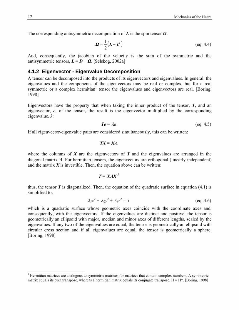
4.1.2 Eigenvector - Eigenvalue Decomposition A tensor can be decomposed into the products of its eigenvectors and eigenvalues. In general, the eigenvalues and the components of the eigenvectors may be real or complex, but for a real symmetric or a complex hermitian1 tensor the eigenvalues and eigenvectors are real. [Boring, 1998] Eigenvectors have the property that when taking the inner product of the tensor, T, and an eigenvector, e, of the tensor, the result is the eigenvector multiplied by the corresponding eigenvalue, λ:
Te = λe (eq. 4.5)
If all eigenvector-eigenvalue pairs are considered simultaneously, this can be written: TX = XΛ where the columns of X are the eigenvectors of T and the eigenvalues are arranged in the diagonal matrix Λ. For hermitian tensors, the eigenvectors are orthogonal (linearly independent) and the matrix X is invertible. Then, the equation above can be written: T = XΛX-1
thus, the tensor T is diagonalized. Then, the equation of the quadratic surface in equation (4.1) is simplified to:
λ1x2 + λ2y2 + λ3z2 = 1 (eq. 4.6)
which is a quadratic surface whose geometric axes coincide with the coordinate axes and, consequently, with the eigenvectors. If the eigenvalues are distinct and positive, the tensor is geometrically an ellipsoid with major, median and minor axes of different lengths, scaled by the eigenvalues. If any two of the eigenvalues are equal, the tensor is geometrically an ellipsoid with circular cross section and if all eigenvalues are equal, the tensor is geometrically a sphere. [Boring, 1998]
1 Hermitian matrices are analogous to symmetric matrices for matrices that contain complex numbers. A symmetric matrix equals its own transpose, whereas a hermitian matrix equals its conjugate transpose, H = H*. [Boring, 1998]

Mechanics of the Heart 13
Invariants The principal invariants of a tensor are related to the tensor quadratic surface. The invariants, I1, I2, I3, for a strain tensor can be written:
I1 = λ1 + λ2 + λ3
I2 = 21 (λ1λ2 + λ2λ3 + λ3λ1)
I3 = ( )32131 λλλ (eq. 4.7)
If the quadratic surface is an ellipsoid, I1 is the sum of the principle axes lengths, I2 is the sum of the cross sectional areas of the three orthogonal slices defined by any two of the principle axes and I3 is the volume of the ellipsoid. Each of these quantities is invariant under a change of coordinate system. [Boring, 1998]
4.2 Strain Strain is a dimensionless parameter describing deformation. Consider a one dimensional elastic beam, see figure 4.1. When applying a force at each of its ends, the beam lengthens. The relation, ε, between the beam’s lengthening, L-L0, and its original length, L0, is defined as the strain along this direction.
0
0
LLL −
=ε (eq. 4.8)
Figure 4.1 shows an elastic beam with original length L0, applied to a force and thus lengthened to the length L.
Figure 4.1 One dimensional strain.
Thus, strain describes the deformation of a body. In three dimensions, the deformation can be described by the following.
L
L0
14 Mechanics of the Heart
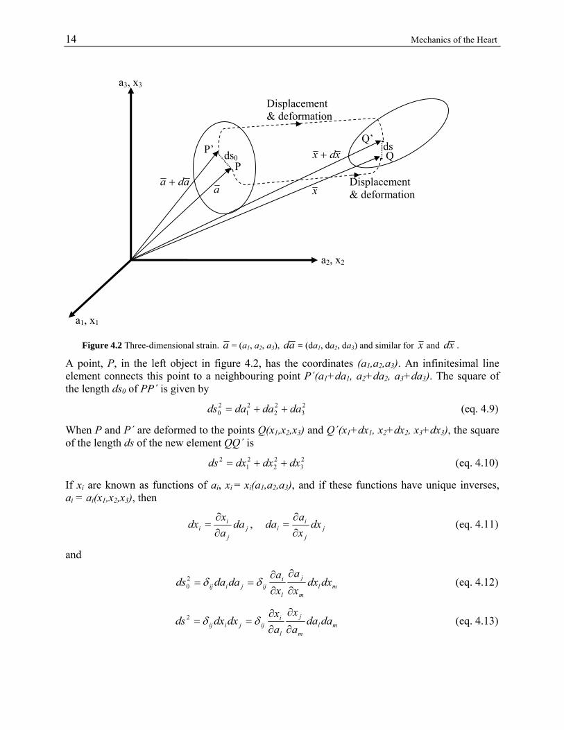
Figure 4.2 Three-dimensional strain. a = (a1, a2, a3), ad = (da1, da2, da3) and similar for x and xd .
A point, P, in the left object in figure 4.2, has the coordinates (a1,a2,a3). An infinitesimal line element connects this point to a neighbouring point P´(a1+da1, a2+da2, a3+da3). The square of the length ds0 of PP´ is given by
23
22
21
20 dadadads ++= (eq. 4.9)
When P and P´ are deformed to the points Q(x1,x2,x3) and Q´(x1+dx1, x2+dx2, x3+dx3), the square of the length ds of the new element QQ´ is
23
22
21
2 dxdxdxds ++= (eq. 4.10)
If xi are known as functions of ai, xi = xi(a1,a2,a3), and if these functions have unique inverses, ai = ai(x1,x2,x3), then
jj
ii da
ax
dx∂∂
= , jj
ii dx
xa
da∂∂
= (eq. 4.11)
and
mlm
j
l
iijjiij dxdx
xa
xa
dadads∂
∂
∂∂
== δδ20 (eq. 4.12)
mlm
j
l
iijjiij dada
ax
ax
dxdxds∂
∂
∂∂
== δδ2 (eq. 4.13)
a2, x2
a3, x3
P’ .
a ada +
x
xdx +. P
ds0
Q’ . . Q ds
Displacement & deformation
Displacement & deformation
a1, x1
Mechanics of the Heart 15
The repetition of indices in the terms above indicate summation over the range of each index
(Einstein’s summation convention) and ⎩⎨⎧
≠=
=jiji
ij ,0,1
δ (Kronecker delta).
The difference between 2
0ds and 2ds may now be written
jiijji
dadaax
ax
dsds ⎟⎟⎠
⎞⎜⎜⎝
⎛−
∂
∂
∂∂
=− δδ βααβ
20
2 (eq. 4.14)
The Lagrangian strain tensor E is in indicial notation defined by
⎟⎟⎠
⎞⎜⎜⎝
⎛−
∂
∂
∂∂
= ijji
ij ax
ax
E δδ βααβ2
1 (eq. 4.15)
and in matrix notation E is defined by
E = 21 (C - I) (eq. 4.16)
where
C = FtF, Cauchy-Green deformation tensor (eq. 4.17)
axF∂∂
= , deformation gradient tensor (eq. 4.18)
The deformation of the body can thus be written
jiij dadaEdsds 220
2 =− (eq. 4.19) The tensor C in (4.17) is called the right Cauchy-Green deformation tensor and it equals the identity matrix I in the absence of motion or for a rigid body motion [Selskog, 2002b]. The subtraction of I in (4.16) takes rigid body motions away. A rigid body motion accomplishes no deformation and the strain tensor E is zero in each tensor element when there is no deformation. [Fung, 1969]
4.2.1 The Determinant of the Strain Tensor Here, the physical interpretations of the determinants of the deformation gradient tensor F and of the strain tensor E are treated. First, the fundamental definition of the determinant. Definition: If V is a vector space and if A is in the set of linear transformations L(V;V), then the determinant of A, detA, is a scalar defined by [Bowen, 1989]:
( ) ( ) ( )AwAvAuwvuA ×⋅=×⋅det (eq. 4.20) A volume can be calculated from three appropriate vectors by use of the scalar triple product, dx(1).(dx(2)×dx(3)). Using the fundamental definition of the determinant, the physical interpretation of the determinant of the deformation gradient tensor, detF, comes out of the following equation, where X(i) are vectors in reference configuration and x(i) in deformed state:
16 Mechanics of the Heart ( ) ( )=⋅×⋅⋅=×⋅= )3()2()1()3()2()1( XFXFXFxxx dddddddv ( ) ( ) dVddd ⋅=×⋅= FXXXF detdet )3()2()1( (eq. 4.21) Thus, detF (= dv/dV) maps original differential volumes into current ones. If the deformation described by F is isochoric (volume preserving), detF = 1 and the material is said to be incompressible. As E = ½(FtF – I), detF = 1 corresponds to detE = 0. Note that the third invariant I3 (4.7) of the strain tensor E is one third of the determinant, and thus I3 = 0 for isochoric deformations. [Humphrey, 2002]
4.2.2 Strain Components of the Cardiac Wall Myocardial strains are expressed as normal and shear strains. The strain tensor components are defined in (4.19). In a local coordinate system, three normal and three shear strains are obtained. Normal strains will deform a cube into a beam, and shear strains will deform it into a parallelepiped. [Bogaert, 2001] Myocardium consists largely of water (intracellular and interstitial water) that is not particularly mobile and the myocardium is thus expected to be incompressible. But the myocardium also includes an extensive vasculature and the blood within the myocardial vasculature is highly mobile. Whereas incompressibility may be assumed in non-perfused tissue, one must account for blood flow related changes in volume in perfused tissue. Thus, the determinant of the strain tensor of perfused tissue is not expected to be exactly zero. [Humphrey, 2002]
Method 17
5 Method An overview of the entire cardiac strain examination is given in appendix A. Here, the kinematical method used in this survey is described. Kinematics is the science of motion, but not just of the motion itself; it is the study of the positions, angles, velocities, and accelerations of segments of a body during motion.
5.1 Cardiac Coordinate System Regardless of the data acquisition method, the coordinate system of the acquired data is relative to a Cartesian laboratory reference frame (Eulerian). Hence, rigid body motions of the heart can be seen in this coordinate system. When analyzing cardiac strain and other parameters within the heart, there is a need for an internal Cartesian reference system (Lagrangian) which is attached to the heart and follows the cardiac movements, i.e. a cardiac coordinate system. The cardiac coordinates are, in this thesis work, circumferential, longitudinal and radial (C, L and R, respectively). The radial direction is normal to the cardiac wall and positive if it points away from the centre of the left ventricle. The circumferential direction is perpendicular to the radial direction and tangential to the cardiac wall, directed counterclockwise in a short axis view seen from superior direction. The longitudinal direction is tangential to the cardiac wall and perpendicular to both the circumferential and the radial direction and directed basally. Specifics on how the cardiac coordinates are implemented for marker and bead data and for PC-MRI data, respectively, are given in appendix B.
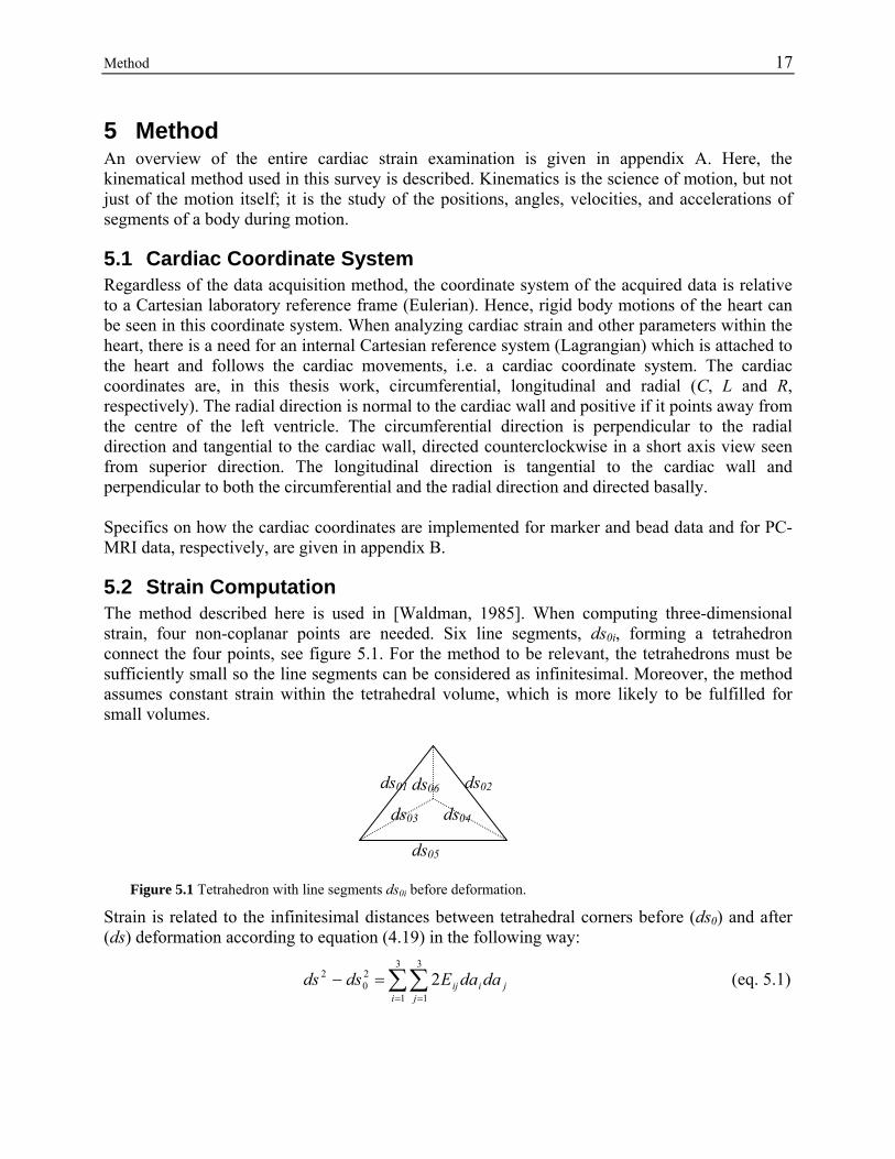
5.2 Strain Computation The method described here is used in [Waldman, 1985]. When computing three-dimensional strain, four non-coplanar points are needed. Six line segments, ds0i, forming a tetrahedron connect the four points, see figure 5.1. For the method to be relevant, the tetrahedrons must be sufficiently small so the line segments can be considered as infinitesimal. Moreover, the method assumes constant strain within the tetrahedral volume, which is more likely to be fulfilled for small volumes.
Figure 5.1 Tetrahedron with line segments ds0i before deformation.
Strain is related to the infinitesimal distances between tetrahedral corners before (ds0) and after (ds) deformation according to equation (4.19) in the following way:
∑∑= =
=−3
1
3
1
20
2 2i j
jiij dadaEdsds (eq. 5.1)
ds05
ds01 ds02
ds03 ds04
ds06
18 Method Here, dai are the infinite coordinate components of the tetrahedral line segments in the reference configuration (before deformation). A finite version of this equation is approximated to be valid for the finite element of the tetrahedron, and it is applied to the six line segments. Hence, a set of six simultaneous linear algebraic equations is solved to calculate the six independent strain components of the symmetric strain tensor at each time step after reference time.
( )( )( )( )( )( )
32144444444444 344444444444 21
4434421
EX
s ⎥⎥⎥⎥⎥⎥⎥⎥
⎦
⎤
⎢⎢⎢⎢⎢⎢⎢⎢
⎣
⎡
⎥⎥⎥⎥⎥⎥⎥⎥
⎦
⎤
⎢⎢⎢⎢⎢⎢⎢⎢
⎣
⎡ ∆∆∆∆∆∆∆∆∆
=
⎥⎥⎥⎥⎥
⎦
⎤
⎢⎢⎢⎢⎢
⎣
⎡
∆−∆
∆−∆
RR
LR
LL
CR
CL
CC
EEEEEEaaaaaaaaa
ss
ss
6
5
4
3
2
12332
223121
21
206
26
201
21
...
...
...
...
...242442
...
... (eq. 5.2)
Since the vectors in equation (5.2) are named s and E and the matrix is named X, the equation can be written: XEs = (eq. 5.3) The strain components can now be found simply by inverting the matrix: sXE 1−= (eq. 5.4) The procedure of strain computation shown above is done in all points and in all time frames where and when strain is sought.
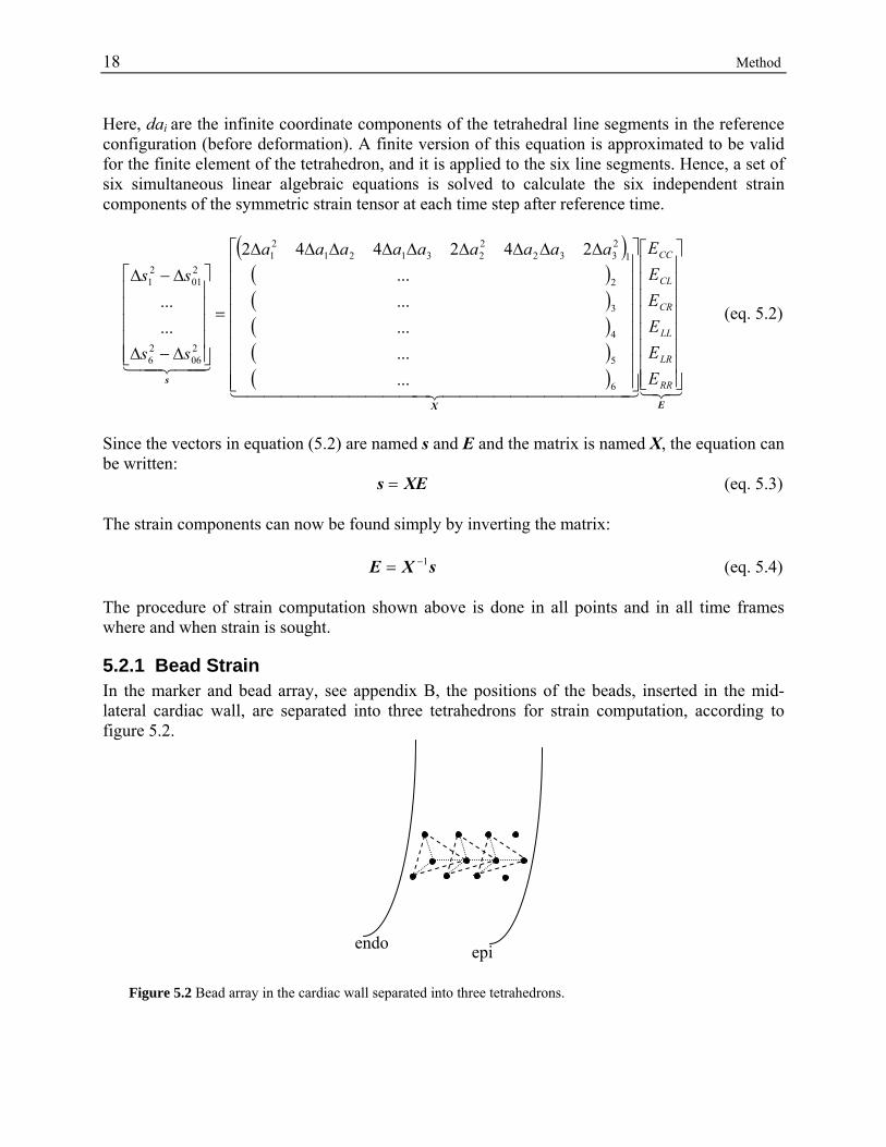
5.2.1 Bead Strain In the marker and bead array, see appendix B, the positions of the beads, inserted in the mid-lateral cardiac wall, are separated into three tetrahedrons for strain computation, according to figure 5.2.
Figure 5.2 Bead array in the cardiac wall separated into three tetrahedrons.
endo epi
Method 19
For each time frame, three strain tensors at different wall depths are received. The reference time frame is the end diastolic time frame when calculating bead strain. Each three-dimensional strain tensor contains three normal strain components and three shear strain components. The strain components are interpolated in the transmural direction in order to achieve transmural strain maps.
Interpolation When interpolating, the position of the centroid of each tetrahedron is projected onto the cardiac radial axis. The length of each projection is computed and the deepest tetrahedron is found as the one with maximum length of projection (Pmax), see figure 5.3.
R
Pmax
Figure 5.3 Tetrahedral centroids projected onto radial axis. Pmax is the length of the projection of the deepest bead.
A vector with 101 components is created, representing 101 positions along the radial axis between –Pmax and zero, with a spacing of Pmax/100. For each strain component, a second order polynomial is fitted to the strain values at the positions of their projections on the radial axis. Then the interpolated strain component is created using the coefficients of the polynomial multiplied with the closely spaced position vector.
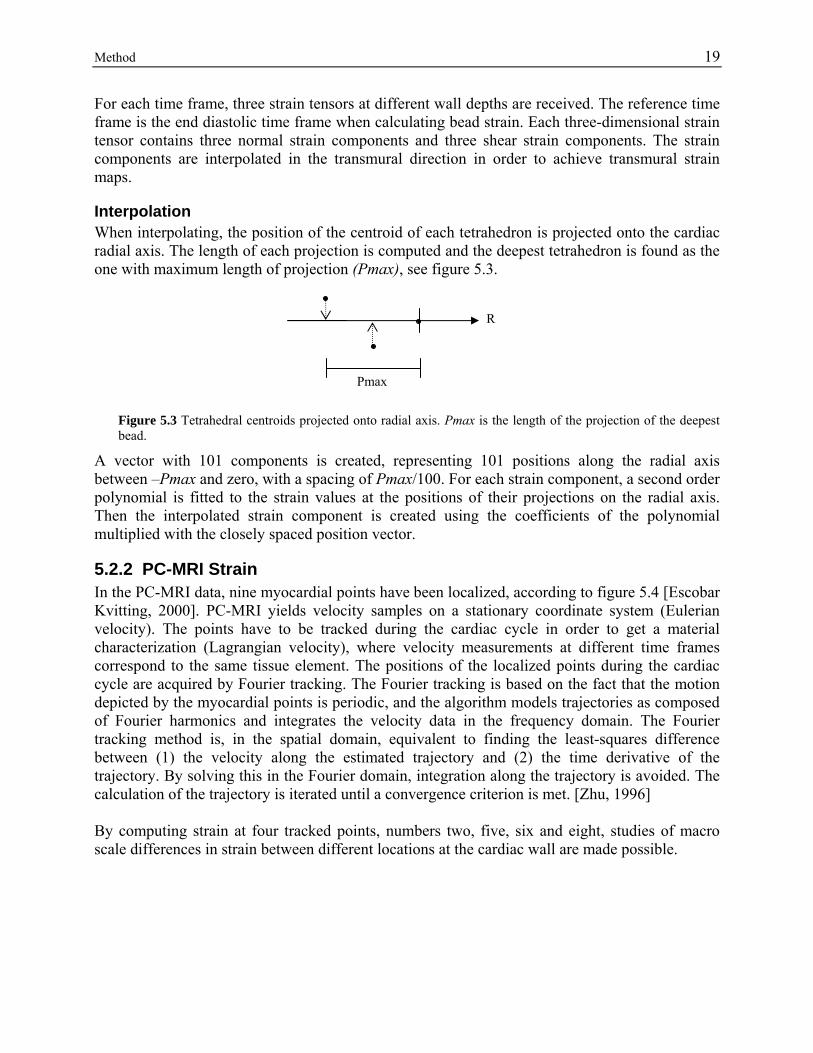
5.2.2 PC-MRI Strain In the PC-MRI data, nine myocardial points have been localized, according to figure 5.4 [Escobar Kvitting, 2000]. PC-MRI yields velocity samples on a stationary coordinate system (Eulerian velocity). The points have to be tracked during the cardiac cycle in order to get a material characterization (Lagrangian velocity), where velocity measurements at different time frames correspond to the same tissue element. The positions of the localized points during the cardiac cycle are acquired by Fourier tracking. The Fourier tracking is based on the fact that the motion depicted by the myocardial points is periodic, and the algorithm models trajectories as composed of Fourier harmonics and integrates the velocity data in the frequency domain. The Fourier tracking method is, in the spatial domain, equivalent to finding the least-squares difference between (1) the velocity along the estimated trajectory and (2) the time derivative of the trajectory. By solving this in the Fourier domain, integration along the trajectory is avoided. The calculation of the trajectory is iterated until a convergence criterion is met. [Zhu, 1996] By computing strain at four tracked points, numbers two, five, six and eight, studies of macro scale differences in strain between different locations at the cardiac wall are made possible.
20 Method
3
4 septal
9 apex
6 anterior
8
5 1
2 lateral
7 posterior
Figure 5.4 Nine tracked points in PC-MRI data.
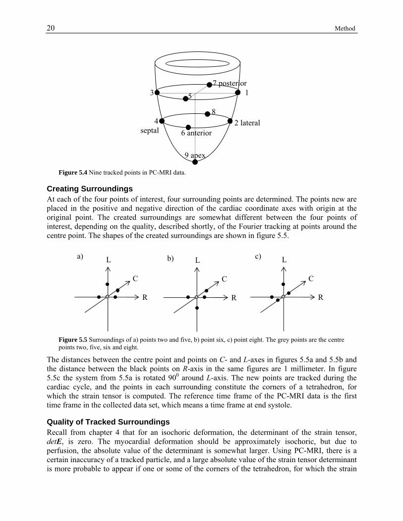
Creating Surroundings At each of the four points of interest, four surrounding points are determined. The points new are placed in the positive and negative direction of the cardiac coordinate axes with origin at the original point. The created surroundings are somewhat different between the four points of interest, depending on the quality, described shortly, of the Fourier tracking at points around the centre point. The shapes of the created surroundings are shown in figure 5.5.
a) c) b)L L L
C C C
R R R
Figure 5.5 Surroundings of a) points two and five, b) point six, c) point eight. The grey points are the centre points two, five, six and eight.
The distances between the centre point and points on C- and L-axes in figures 5.5a and 5.5b and the distance between the black points on R-axis in the same figures are 1 millimeter. In figure 5.5c the system from 5.5a is rotated 900 around L-axis. The new points are tracked during the cardiac cycle, and the points in each surrounding constitute the corners of a tetrahedron, for which the strain tensor is computed. The reference time frame of the PC-MRI data is the first time frame in the collected data set, which means a time frame at end systole.
Quality of Tracked Surroundings Recall from chapter 4 that for an isochoric deformation, the determinant of the strain tensor, detE, is zero. The myocardial deformation should be approximately isochoric, but due to perfusion, the absolute value of the determinant is somewhat larger. Using PC-MRI, there is a certain inaccuracy of a tracked particle, and a large absolute value of the strain tensor determinant is more probable to appear if one or some of the corners of the tetrahedron, for which the strain

Method 21
tensor is computed, is not myocardial. Hence, the strain tensor determinant can be used as a measure of inaccuracy of the strain tensor. The determinant of the strain tensor of each region is computed and evaluated. The final surroundings are those with smallest absolute values of their determinants, among the tested surroundings of each region. For the final surroundings, shown in figure 5.5, the strain tensor components are plotted and compared, acquiring macro scale differences in myocardial strain.
5.2.3 Comparison of Bead and PC-MRI Strain The results of bead strain computation and of PC-MRI strain computation are compared, by plotting the derived strain from the mid-wall bead tetrahedron in the same plot as the strain of PC-MRI the lateral region (2), which is the MRI region closest to the corresponding position of the bead array. In the plot, the chosen time interval of the cardiac cycle is the same as the time interval during PC-MRI strain computation, i.e. starting at end systole and continuing one cardiac cycle ahead, using the end systolic time frame as reference.

22 Method

Results 23
6 Results Here, the results of bead strain and of PC-MRI strain computation are presented. The bead strain results are presented both as time plots of each strain component from the sub-endocardial tetrahedron and as transmural strain maps. For PC-MRI strain, the values of the determinants of the strain tensors during the cardiac cycle are presented, as well as plots of each strain tensor component for all four regions, which are useful in macro scale analysis of strain. At last, a comparison of the bead strain results and the PC-MRI strain results is given.
6.1 Bead Strain The strain components from the sub-endocardial tetrahedron are plotted in figure 6.1. In the same figure, the comparable canine sub-endocardial strain results from [Waldman, 1985] are shown. The results of Waldman are computed by the same method as in this survey but using a canine heart, and are taken from a tetrahedron whose centroid was located in the inner third of the left ventricular lateral wall. The volume curve corresponding to the studied time interval is shown to the left of each transmural strain map in figure 6.2, an interval of one cardiac cycle starting just before end diastole. In figure 6.1, the circumferential normal strain reaches a minimum and the radial normal strain reaches a maximum at end systole. The other strain components are in this example minimal.
10 20 30 40 50-0.2
-0.1
0
0.1
0.2ECC
10 20 30 40 50-0.3
-0.2-0.1
00.1
0.20.3
ELL
10 20 30 40 50-0.5
0
0.5
1ERR
10 20 30 40 50-0.2
-0.1
0
0.1
0.2ECL
10 20 30 40 50-0.2
0
0.2
0.40.5
ECR
10 20 30 40 50-0.4
-0.2
0
0.2
0.4ELR
Figure 6.1 The sub-endocardial strain components are plotted during the cardiac cycle. As a comparison, approximate strain values from [Waldman, 1985] are shown as circles. The values of the strain components are on vertical axes and time frames are shown on horizontal axes. Note that there are different scales on the vertical axes.
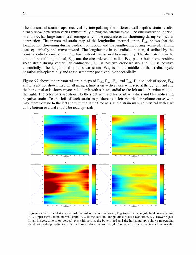
24 Results The transmural strain maps, received by interpolating the different wall depth’s strain results, clearly show how strain varies transmurally during the cardiac cycle. The circumferential normal strain, ECC, has large transmural homogeneity in the circumferential shortening during ventricular contraction. The transmural strain map of the longitudinal normal strain, ELL, shows that the longitudinal shortening during cardiac contraction and the lengthening during ventricular filling start epicardially and move inward. The lengthening in the radial direction, described by the positive radial normal strain, ERR, has moderate transmural homogeneity. The shear strains in the circumferential-longitudinal, ECL, and the circumferential-radial, ECR, planes both show positive shear strain during ventricular contraction; ECL is positive endocardially and ECR is positive epicardially. The longitudinal-radial shear strain, ELR, is in the middle of the cardiac cycle negative sub-epicardially and at the same time positive sub-endocardially. Figure 6.2 shows the transmural strain maps of ECC, ELL, ERR and ELR. Due to lack of space, ECL and ECR are not shown here. In all images, time is on vertical axis with zero at the bottom end and the horizontal axis shows myocardial depth with sub-epicardial to the left and sub-endocardial to the right. The color bars are shown to the right with red for positive values and blue indicating negative strain. To the left of each strain map, there is a left ventricular volume curve with maximum volume to the left and with the same time axis as the strain map, i.e. vertical with start at the bottom end and should be read upwards.
volume
wall depth [%]
ECC
10 20 30 40 50 60 70 80 90 100
10
15
20
25
30
35
40
45
50
-0.2
-0.15
-0.1
-0.05
0
0.05
0.1
0.15
0.2volume
wall depth [%]
ELL
10 20 30 40 50 60 70 80 90 100
10
15
20
25
30
35
40
45
50
-0.2
-0.15
-0.1
-0.05
0
0.05
0.1
0.15
0.2
volume
wall depth [%]
ERR
10 20 30 40 50 60 70 80 90 100
10
15
20
25
30
35
40
45
50
-0.2
-0.15
-0.1
-0.05
0
0.05
0.1
0.15
0.2volume
wall depth [%]
ELR
10 20 30 40 50 60 70 80 90 100
10
15
20
25
30
35
40
45
50
-0.2
-0.15
-0.1
-0.05
0
0.05
0.1
0.15
0.2
Figure 6.2 Transmural strain maps of circumferential normal strain, ECC, (upper left), longitudinal normal strain, ELL, (upper right), radial normal strain, ERR, (lower left) and longitudinal-radial shear strain, ELR, (lower right). In all images, time is on vertical axis with zero at the bottom end and the horizontal axis shows myocardial depth with sub-epicardial to the left and sub-endocardial to the right. To the left of each map is a left ventricular
Results 25
volume curve with the same time axis as the strain map, maximum volume to the left and minimum volume to the right.
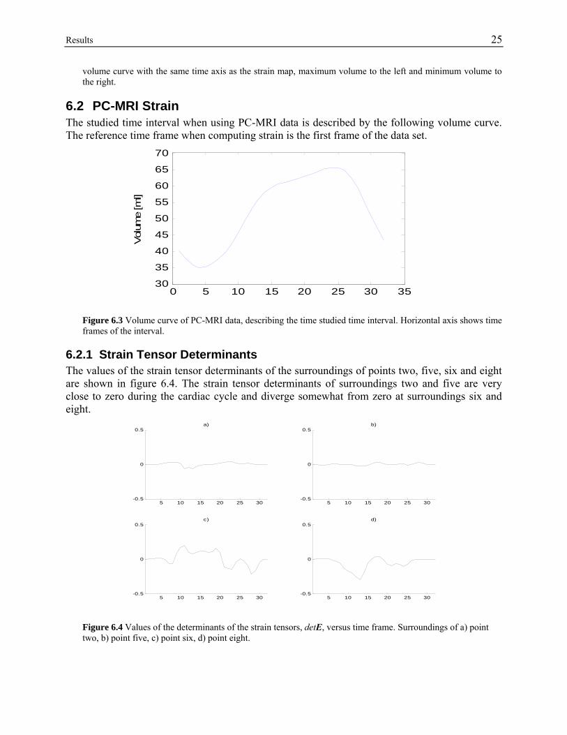
6.2 PC-MRI Strain The studied time interval when using PC-MRI data is described by the following volume curve. The reference time frame when computing strain is the first frame of the data set.
0 5 10 15 20 25 30 3530
35
40
45
50
55
60
65
70
Vol
ume
[ml]
Figure 6.3 Volume curve of PC-MRI data, describing the time studied time interval. Horizontal axis shows time frames of the interval.
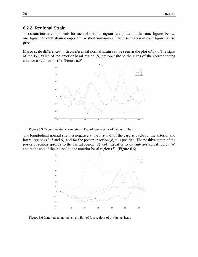
6.2.1 Strain Tensor Determinants The values of the strain tensor determinants of the surroundings of points two, five, six and eight are shown in figure 6.4. The strain tensor determinants of surroundings two and five are very close to zero during the cardiac cycle and diverge somewhat from zero at surroundings six and eight.
5 10 15 20 25 30-0.5
0
0.5a)
5 10 15 20 25 30-0.5
0
0.5b)
5 10 15 20 25 30-0.5
0
0.5c)
5 10 15 20 25 30-0.5
0
0.5d)
Figure 6.4 Values of the determinants of the strain tensors, detE, versus time frame. Surroundings of a) point two, b) point five, c) point six, d) point eight.
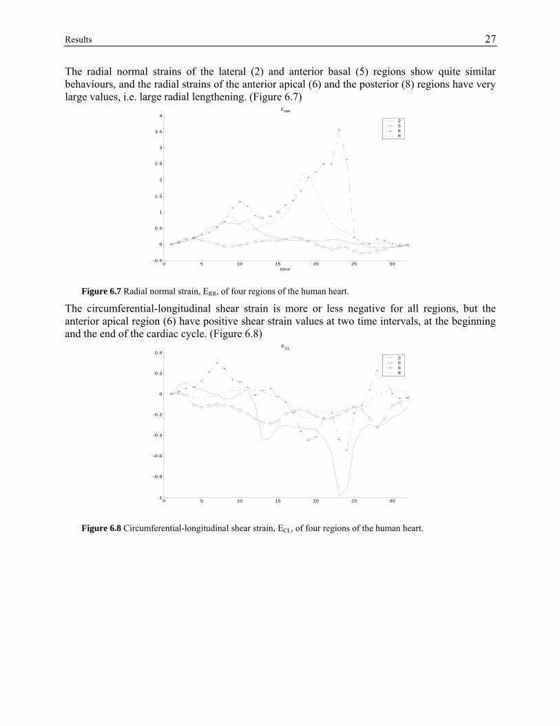
26 Results 6.2.2 Regional Strain The strain tensor components for each of the four regions are plotted in the same figures below, one figure for each strain component. A short summary of the results seen in each figure is also given. Macro scale differences in circumferential normal strain can be seen in the plot of ECC. The signs of the ECC value of the anterior basal region (5) are opposite to the signs of the corresponding anterior apical region (6). (Figure 6.5)
0 5 10 15 20 25 30-0.6
-0.4
-0.2
0
0.2
0.4
0.6
0.8ECC
2568
Figure 6.5 Circumferential normal strain, ECC, of four regions of the human heart.
The longitudinal normal strain is negative at the first half of the cardiac cycle for the anterior and lateral regions (2, 5 and 6), and for the posterior region (8) it is positive. The positive strain of the posterior region spreads to the lateral region (2) and thereafter to the anterior apical region (6) and at the end of the interval to the anterior basal region (5). (Figure 6.6)
0 5 10 15 20 25 30-0.6
-0.4
-0.2
0
0.2
0.4
0.6
0.8
1
1.2
1.4ELL
2568
Figure 6.6 Longitudinal normal strain, ELL, of four regions of the human heart.
Results 27
The radial normal strains of the lateral (2) and anterior basal (5) regions show quite similar behaviours, and the radial strains of the anterior apical (6) and the posterior (8) regions have very large values, i.e. large radial lengthening. (Figure 6.7)
0 5 10 15 20 25 30-0.5
0
0.5
1
1.5
2
2.5
3
3.5
4ERR
time
2568
Figure 6.7 Radial normal strain, ERR, of four regions of the human heart.
The circumferential-longitudinal shear strain is more or less negative for all regions, but the anterior apical region (6) have positive shear strain values at two time intervals, at the beginning and the end of the cardiac cycle. (Figure 6.8)
0 5 10 15 20 25 30-1
-0.8
-0.6
-0.4
-0.2
0
0.2
0.4ECL
2568
Figure 6.8 Circumferential-longitudinal shear strain, ECL, of four regions of the human heart.
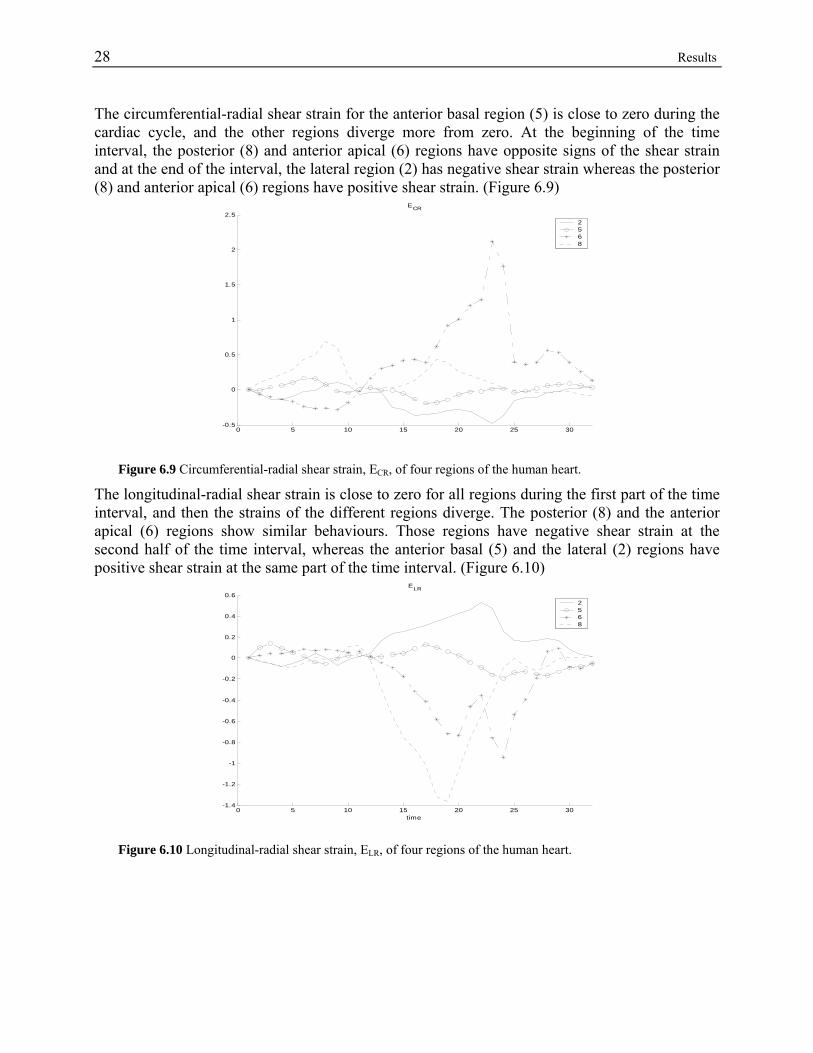
28 Results The circumferential-radial shear strain for the anterior basal region (5) is close to zero during the cardiac cycle, and the other regions diverge more from zero. At the beginning of the time interval, the posterior (8) and anterior apical (6) regions have opposite signs of the shear strain and at the end of the interval, the lateral region (2) has negative shear strain whereas the posterior (8) and anterior apical (6) regions have positive shear strain. (Figure 6.9)
0 5 10 15 20 25 30-0.5
0
0.5
1
1.5
2
2.5ECR
2568
Figure 6.9 Circumferential-radial shear strain, ECR, of four regions of the human heart.
The longitudinal-radial shear strain is close to zero for all regions during the first part of the time interval, and then the strains of the different regions diverge. The posterior (8) and the anterior apical (6) regions show similar behaviours. Those regions have negative shear strain at the second half of the time interval, whereas the anterior basal (5) and the lateral (2) regions have positive shear strain at the same part of the time interval. (Figure 6.10)
0 5 10 15 20 25 30-1.4
-1.2
-1
-0.8
-0.6
-0.4
-0.2
0
0.2
0.4
0.6ELR
time
2568
Figure 6.10 Longitudinal-radial shear strain, ELR, of four regions of the human heart.
Results 29
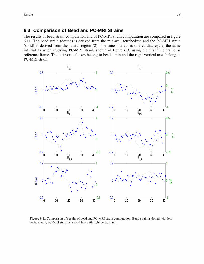
6.3 Comparison of Bead and PC-MRI Strains The results of bead strain computation and of PC-MRI strain computation are compared in figure 6.11. The bead strain (dotted) is derived from the mid-wall tetrahedron and the PC-MRI strain (solid) is derived from the lateral region (2). The time interval is one cardiac cycle, the same interval as when studying PC-MRI strain, shown in figure 6.3, using the first time frame as reference frame. The left vertical axes belong to bead strain and the right vertical axes belong to PC-MRI strain.
0 10 20 30 40-0.5
0
0.5
Bea
d
ECC
0 10 20 30 40-1
0
1
0 10 20 30 40-0.2
0
0.2
Bea
d
ELL
0 10 20 30 40-0.6
0
1
0 10 20 30 40-0.2
0
0.2
Bea
d
ERR
0 10 20 30 40-0.6
0
1
0 10 20 30 40-0.2
0
0.2ECL
0 10 20 30 40-1
0
0.6
MR
0 10 20 30 40-0.2
0
0.2ECR
0 10 20 30 40-0.5
0
0.5
MR
0 10 20 30 40-0.2
0
0.2ELR
0 10 20 30 40-1
0
1
MR
Figure 6.11 Comparison of results of bead and PC-MRI strain computation. Bead strain is dotted with left vertical axis, PC-MRI strain is a solid line with right vertical axis.

30 Results
Discussion 31
7 Discussion In this thesis work, strain calculation tools are developed, for both bead strain computation and for PC-MRI strain computation. The tools are useful in future research in this area, suggested in chapter 8. In addition to the developed methods, some results are received. Since only one subject is studied with marker technique and with PC-MRI, respectively, the achieved results can not be considered to be of general validity, but the tendency of the results may hold even in further studies. Here, the results from bead strain computation and from PC-MRI strain computation are discussed, as well as the comparison between bead strain and PC-MRI strain. There is also a discussion of alternative strain computation methods.
7.1 Bead Strain The plot of sub-endocardial strain components versus time frame in figure 6.1 reveals a very good agreement between the received ovine sub-endocardial strain and the results of [Waldman, 1985], although Waldman’s results are derived from canine hearts and although the beads used in this thesis work may not be placed on exactly the same positions as the beads used in [Waldman, 1985]. The kind of visualization used in figure 6.1 is commonly used in strain research articles [Waldman, 1985, Bogaert, 2001] and it gives a detailed description of the strain in one particular region. It is useful when comparing results from different subjects or studies. But the large transmural differences in strain, shown by the transmural strain maps, make a special emphasis on the relevance of localization of the region, from which the results are derived. That is, are the results from a sub-endo, mid-wall or sub-epi region? The transmural strain maps are a new way of visualizing myocardial strain. They are first derived in this thesis work, and have not yet been seen elsewhere. The maps show strain from all transmural depths and from the whole cardiac cycle at the same time and are therefore very useful when surveying myocardial strain. But there has to be some considering on how to visualize standard deviations in these kind of maps, in studies with several subjects. The appearances of the transmural strain maps are dependent on the interpolation method, since strain results are only received at a few cardiac wall depths, in this case at three depths, and the maps use strain interpolated and re-sampled to 101 depths. The interpolation method used in this thesis work fits a second order polynomial to the strain results. The polynomial is chosen to be of second order, because it gives a smoother and more realistic result than a first order polynomial, and fitting of higher order polynomial than the second order results in not unique solutions, since there are only three points/values on which the polynomial is fitted. Inserting more beads in each bead column renders the possibility to choose order of the polynomial during interpolation, and then research has to be done on which order is the best. The marker and bead technique of strain calculation renders, due to the high spatial resolution, the possibility of deriving very detailed transmural strain maps, discussed above. On the other hand, the strain maps can only be created at the place where the beads are inserted, and hence a transmural strain map of the whole heart is not possible to derive, unless beads are inserted
32 Discussion everywhere in the cardiac wall. Another problem with this technique is that the surgical implant of markers and beads may cause scars in the tissue and hence artifacts in the strain results. The invasiveness also makes the technique unusable on humans, and when receiving the results, the fact that they are not human must be considered. The comparison between bead and PC-MRI strain, discussed in a larger extent below, however shows a large similarity between the ovine and the human myocardial strain results of this thesis work. This may authorize detailed surveying of myocardial strain on ovine hearts to get a better knowledge of myocardial strain on humans.
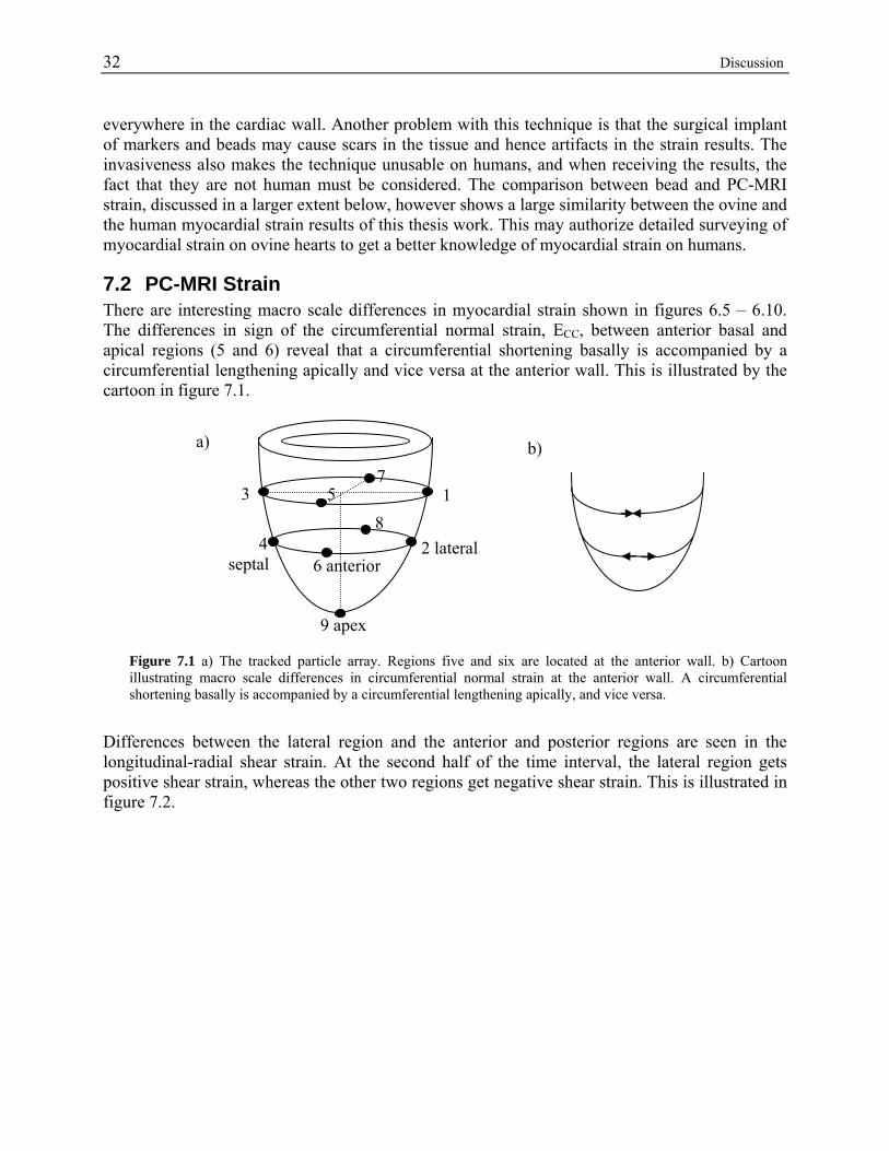
7.2 PC-MRI Strain There are interesting macro scale differences in myocardial strain shown in figures 6.5 – 6.10. The differences in sign of the circumferential normal strain, ECC, between anterior basal and apical regions (5 and 6) reveal that a circumferential shortening basally is accompanied by a circumferential lengthening apically and vice versa at the anterior wall. This is illustrated by the cartoon in figure 7.1.
b)
6 anterior
8 5 1
7
2 lateral 4 septal
9 apex
a)
3
Figure 7.1 a) The tracked particle array. Regions five and six are located at the anterior wall. b) Cartoon illustrating macro scale differences in circumferential normal strain at the anterior wall. A circumferential shortening basally is accompanied by a circumferential lengthening apically, and vice versa.
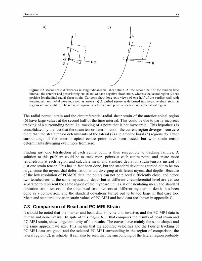
Differences between the lateral region and the anterior and posterior regions are seen in the longitudinal-radial shear strain. At the second half of the time interval, the lateral region gets positive shear strain, whereas the other two regions get negative shear strain. This is illustrated in figure 7.2.
Discussion 33
a) b)
6 or 8
L
R
L
2 R
Figure 7.2 Macro scale differences in longitudinal-radial shear strain. At the second half of the studied time interval, the anterior and posterior regions (6 and 8) have negative shear strain, whereas the lateral region (2) has positive longitudinal-radial shear strain. Cartoons show long axis views of one half of the cardiac wall with longitudinal and radial axes indicated as arrows. a) A dashed square is deformed into negative shear strain at regions six and eight. b) The reference square is deformed into positive shear strain at the lateral region.
The radial normal strain and the circumferential-radial shear strain of the anterior apical region (6) have large values at the second half of the time interval. This could be due to partly incorrect tracking of a surrounding point, i.e. tracking of a point that is not myocardial. This hypothesis is consolidated by the fact that the strain tensor determinant of the current region diverges from zero more than the strain tensor determinants of the lateral (2) and anterior basal (5) regions do. Other surroundings of the anterior apical centre point have been tested, but with strain tensor determinants diverging even more from zero. Finding just one tetrahedron at each centre point is thus susceptible to tracking failures. A solution to this problem could be to track more points at each centre point, and create more tetrahedrons at each region and calculate mean and standard deviation strain tensors instead of just one strain tensor. This has in fact been done, but the standard deviations turned out to be too large, since the myocardial deformation is too diverging at different myocardial depths. Because of the low resolution of PC-MRI data, the points can not be placed sufficiently close, and hence two tetrahedrons at the same myocardial depth but at different circumferential level are yet too separated to represent the same region of the myocardium. Trial of calculating mean and standard deviation strain tensors of the three bead strain tensors at different myocardial depths has been done as a comparison, and the standard deviations turned out to be too large in that case too. Mean and standard deviation strain values of PC-MRI and bead data are shown in appendix C.
7.3 Comparison of Bead and PC-MRI Strain It should be noted that the marker and bead data is ovine and invasive, and the PC-MRI data is human and non-invasive. In spite of this, figure 6.11 that compares the results of bead strain and PC-MRI strain, show large similarity of the results. The curves have mainly the same shapes and the same approximate size. This means that the acquired velocities and the Fourier tracking of PC-MRI data are good, and the selected PC-MRI surrounding in the region of comparison, the lateral region (2), is reliable. It can also be seen that the surrounding of the lateral region probably
34 Discussion is in the middle of the cardiac wall, since the bead tetrahedron used in this plot is the one in the middle of the wall. Since the transmural strain maps of bead strain have shown that the strain is not constant transmurally, selecting bead strain results from another wall depth would give completely different results.
7.4 Alternative Strain Computation Methods In this survey, a finite strain computation method, described by [Waldman, 1985], is used. There are more possible ways of computing strain and all methods may have their own advantages and disadvantages. Some advantages of the method used in this survey are that the strain is computed directly from the definition of strain, and only scalar lengths need be updated in the deformed frames. The disadvantage of the method is, on the other hand, that strain is approximated to be constant within the tetrahedron where it is determined. In the case of PC-MRI, where the resolution is low and thus the selected tetrahedrons are rather large, maybe the approximation of constant strain within the volume is too rough and some other strain computation method may be better adjusted to this case. It is, however, beyond the scope of this thesis to find this other strain computation method. An alternative way of computing the strain tensor is to first compute the deformation gradient tensor F, using a finite version of equation (4.18):
aFx ∆=∆ (eq. 7.1)
With the knowledge of a∆ in a reference configuration and x∆ in a deformed configuration, the deformation gradient tensor F can be computed by solving a 2x2 linear algebraic problem for the two dimensional case and a 3x3 linear algebraic problem for the three-dimensional case. This has been done in two dimensions in [Meier, 1980] and extended to three dimensions in [Waldman, 1985]. Once having F, the Lagrangian strain tensor E can be computed by equation (4.16). In [Waldman, 1985] this strain tensor computation method has been compared to the computation method used in this thesis work, and the results have been proven identical. There are alternative measures of deformation; the Lagrangian strain tensor is not the only measure. The right Cauchy-Green deformation tensor C = FtF (equation 4.17) is a deformation measure further explained in [Selskog, 2002b], and in [Meier, 1980] the deformation gradient tensor F is decomposed into a rotation matrix R and a stretch operator D, F = RD, where D contains all the information on the change in segment size and R describes a local twist in the segment. It is far beyond the scope of this thesis to explain this in detail or to unravel all existing deformation measures.
Future Work 35
8 Future Work Here some topics are discussed, which in future works could improve the results from this thesis work.
8.1 Several Normal Subjects Doing the same kinds of bead strain computation and PC-MRI strain computation as in this thesis work but on several normal subjects, would be of interest to achieve statistically significant results both on the transmural strain maps from bead strain and on the PC-MRI macro scale differences in myocardial strain.
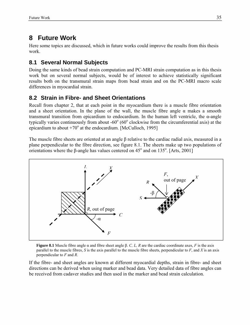
8.2 Strain in Fibre- and Sheet Orientations Recall from chapter 2, that at each point in the myocardium there is a muscle fibre orientation and a sheet orientation. In the plane of the wall, the muscle fibre angle α makes a smooth transmural transition from epicardium to endocardium. In the human left ventricle, the α-angle typically varies continuously from about -60o (60o clockwise from the circumferential axis) at the epicardium to about +70o at the endocardium. [McCulloch, 1995] The muscle fibre sheets are oriented at an angle β relative to the cardiac radial axis, measured in a plane perpendicular to the fibre direction, see figure 8.1. The sheets make up two populations of orientations where the β-angle has values centered on 45o and on 135o. [Arts, 2001]
Figure 8.1 Muscle fibre angle α and fibre sheet angle β. C, L, R are the cardiac coordinate axes, F is the axis parallel to the muscle fibres, S is the axis parallel to the muscle fibre sheets, perpendicular to F, and X is an axis perpendicular to F and R.
If the fibre- and sheet angles are known at different myocardial depths, strain in fibre- and sheet directions can be derived when using marker and bead data. Very detailed data of fibre angles can be received from cadaver studies and then used in the marker and bead strain calculation.
-α
F
C
L X
R, out of page
XR
S-β
F, out of page
36 Future Work 8.2.1 Higher Resolution of PC-MRI When dealing with PC-MRI data, the resolution of this laboratory today is too low for studying strain in fibre- and sheet directions. With a higher resolution, however, the strain in fibre- and sheet directions can be determined. The fibre orientations have in earlier studies [Tseng, 2000] been determined with diffusion sensitive magnetic resonance. Using high resolution PC-MRI and diffusion sensitive MRI, the strain in fibre- and sheet orientations can be determined non-invasively on human beings. This way, the fibre orientations can be determined on the same subject and at the same time as the data for strain computation is acquired. This would give a possibility of creating transmural strain maps of the whole human heart in both local cardiac coordinates and in fibre- and sheet directions.
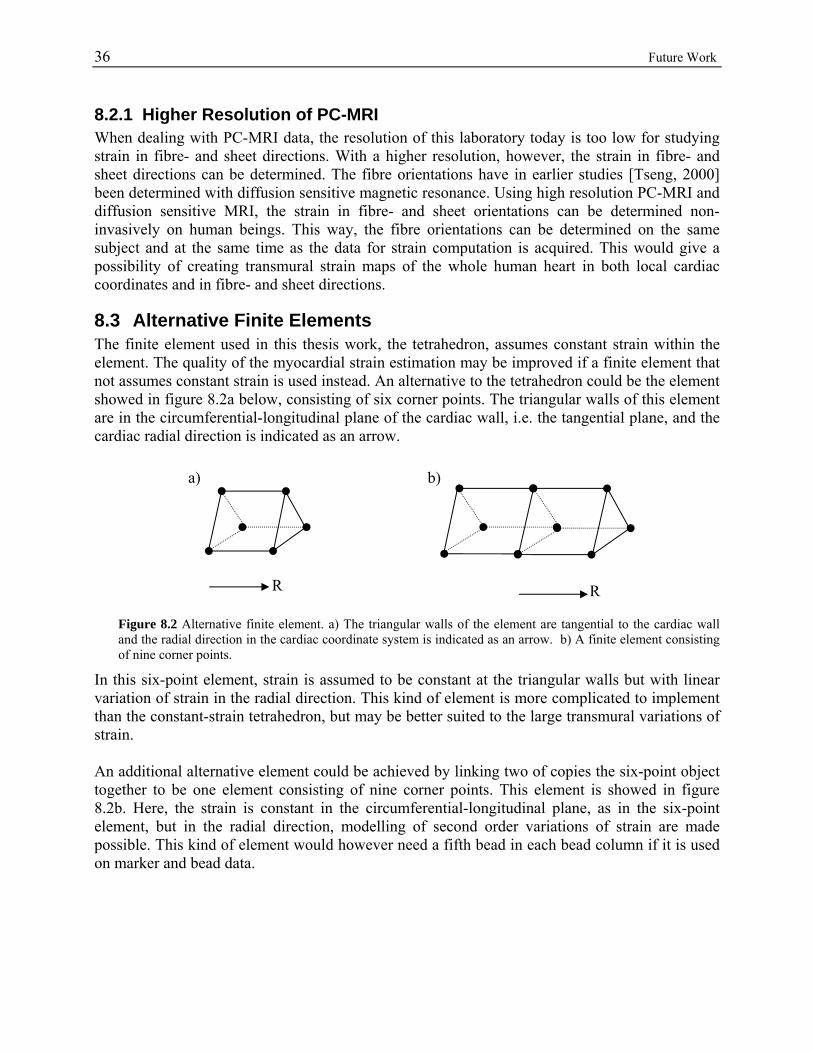
8.3 Alternative Finite Elements The finite element used in this thesis work, the tetrahedron, assumes constant strain within the element. The quality of the myocardial strain estimation may be improved if a finite element that not assumes constant strain is used instead. An alternative to the tetrahedron could be the element showed in figure 8.2a below, consisting of six corner points. The triangular walls of this element are in the circumferential-longitudinal plane of the cardiac wall, i.e. the tangential plane, and the cardiac radial direction is indicated as an arrow.
a)
R
b)
R
Figure 8.2 Alternative finite element. a) The triangular walls of the element are tangential to the cardiac wall and the radial direction in the cardiac coordinate system is indicated as an arrow. b) A finite element consisting of nine corner points.
In this six-point element, strain is assumed to be constant at the triangular walls but with linear variation of strain in the radial direction. This kind of element is more complicated to implement than the constant-strain tetrahedron, but may be better suited to the large transmural variations of strain. An additional alternative element could be achieved by linking two of copies the six-point object together to be one element consisting of nine corner points. This element is showed in figure 8.2b. Here, the strain is constant in the circumferential-longitudinal plane, as in the six-point element, but in the radial direction, modelling of second order variations of strain are made possible. This kind of element would however need a fifth bead in each bead column if it is used on marker and bead data.
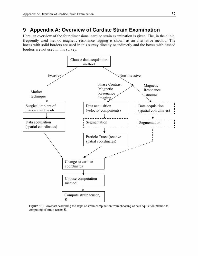
Appendix A: Overview of Cardiac Strain Examination 37
9 Appendix A: Overview of Cardiac Strain Examination Here, an overview of the four dimensional cardiac strain examination is given. The, in the clinic, frequently used method magnetic resonance tagging is shown as an alternative method. The boxes with solid borders are used in this survey directly or indirectly and the boxes with dashed borders are not used in this survey.
Magnetic Resonance Tagging
Choose data acquisition method
Phase Contrast Magnetic Resonance Imaging
Marker technique
Non-Invasive Invasive
Data acquisition (velocity components)
Surgical implant of markers and beads
Data acquisition (spatial coordinates)
Segmentation
Particle Trace (receive spatial coordinates)
Change to cardiac coordinates
Choose computation method
Data acquisition (spatial coordinates)
Segmentation
Compute strain tensor, E
Figure 9.1 Flowchart describing the steps of strain computation,from choosing of data aquisition method to computing of strain tensor E.
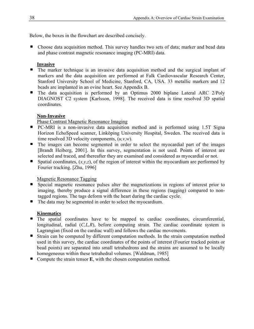
38 Appendix A: Overview of Cardiac Strain Examination Below, the boxes in the flowchart are described concisely.
Choose data acquisition method. This survey handles two sets of data; marker and bead data and phase contrast magnetic resonance imaging (PC-MRI) data.
Invasive
The marker technique is an invasive data acquisition method and the surgical implant of markers and the data acquisition are performed at Falk Cardiovascular Research Center, Stanford University School of Medicine, Stanford, CA, USA. 33 metallic markers and 12 beads are implanted in an ovine heart. See Appendix B.
The data acquisition is performed by an Optimus 2000 biplane Lateral ARC 2/Poly DIAGNOST C2 system [Karlsson, 1998]. The received data is time resolved 3D spatial coordinates.
Non-Invasive Phase Contrast Magnetic Resonance Imaging
PC-MRI is a non-invasive data acquisition method and is performed using 1.5T Signa Horizon EchoSpeed scanner, Linköping University Hospital, Sweden. The received data is time resolved 3D velocity components, (u,v,w).
The images can become segmented in order to select the myocardial part of the images [Brandt Heiberg, 2001]. In this survey, segmentation is not used. Points of interest are selected and traced, and thereafter they are examined and considered as myocardial or not.
Spatial coordinates, (x,y,z), of the region of interest within the myocardium are performed by Fourier tracking. [Zhu, 1996]
Magnetic Resonance Tagging
Special magnetic resonance pulses alter the magnetizations in regions of interest prior to imaging, thereby produce a signal difference in these regions (tagging) compared to non-tagged regions. The tags deform with the heart during the cardiac cycle.
The data may be segmented in order to select the myocardium. Kinematics
The spatial coordinates have to be mapped to cardiac coordinates, circumferential, longitudinal, radial (C,L,R), before computing strain. The cardiac coordinate system is Lagrangian (fixed on the cardiac wall) and follows the cardiac movements.
Strain can be computed by different computation methods. In the strain computation method used in this survey, the cardiac coordinates of the points of interest (Fourier tracked points or bead points) are separated into small tetrahedrons and the strains are assumed to be locally homogeneous within these tetrahedral volumes. [Waldman, 1985]
Compute the strain tensor E, with the chosen computation method.
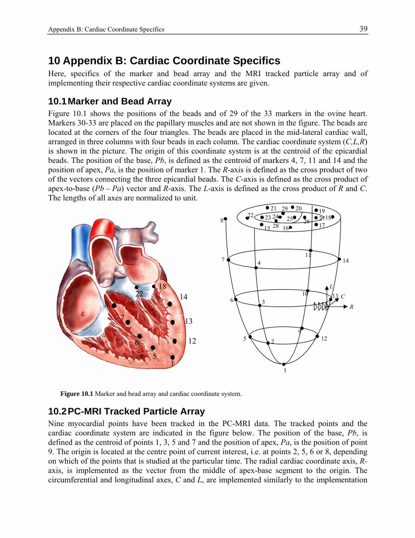
Appendix B: Cardiac Coordinate Specifics 39
10 Appendix B: Cardiac Coordinate Specifics Here, specifics of the marker and bead array and the MRI tracked particle array and of implementing their respective cardiac coordinate systems are given.
10.1 Marker and Bead Array Figure 10.1 shows the positions of the beads and of 29 of the 33 markers in the ovine heart. Markers 30-33 are placed on the papillary muscles and are not shown in the figure. The beads are located at the corners of the four triangles. The beads are placed in the mid-lateral cardiac wall, arranged in three columns with four beads in each column. The cardiac coordinate system (C,L,R) is shown in the picture. The origin of this coordinate system is at the centroid of the epicardial beads. The position of the base, Pb, is defined as the centroid of markers 4, 7, 11 and 14 and the position of apex, Pa, is the position of marker 1. The R-axis is defined as the cross product of two of the vectors connecting the three epicardial beads. The C-axis is defined as the cross product of apex-to-base (Pb – Pa) vector and R-axis. The L-axis is defined as the cross product of R and C. The lengths of all axes are normalized to unit.
R
L
C
22
17 1
19 27 8
15 16
20 21 29
28 25 26 23 24
14
13
11
10
9 12
8
7
6
5
4
2
3
1
22 18
7
6
5 1
14 8
13
12
Figure 10.1 Marker and bead array and cardiac coordinate system.
10.2 PC-MRI Tracked Particle Array Nine myocardial points have been tracked in the PC-MRI data. The tracked points and the cardiac coordinate system are indicated in the figure below. The position of the base, Pb, is defined as the centroid of points 1, 3, 5 and 7 and the position of apex, Pa, is the position of point 9. The origin is located at the centre point of current interest, i.e. at points 2, 5, 6 or 8, depending on which of the points that is studied at the particular time. The radial cardiac coordinate axis, R-axis, is implemented as the vector from the middle of apex-base segment to the origin. The circumferential and longitudinal axes, C and L, are implemented similarly to the implementation
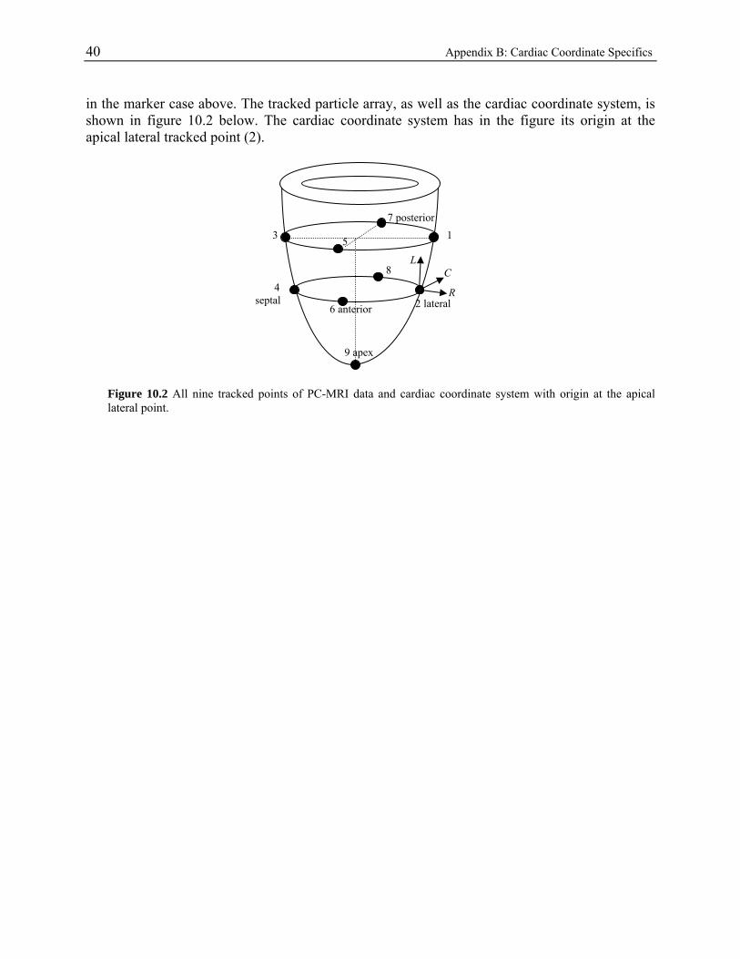
40 Appendix B: Cardiac Coordinate Specifics in the marker case above. The tracked particle array, as well as the cardiac coordinate system, is shown in figure 10.2 below. The cardiac coordinate system has in the figure its origin at the apical lateral tracked point (2).
L C
2 lateral R
7 posterior 1 3
8 4 septal
9 apex
6 anterior
5
Figure 10.2 All nine tracked points of PC-MRI data and cardiac coordinate system with origin at the apical lateral point.
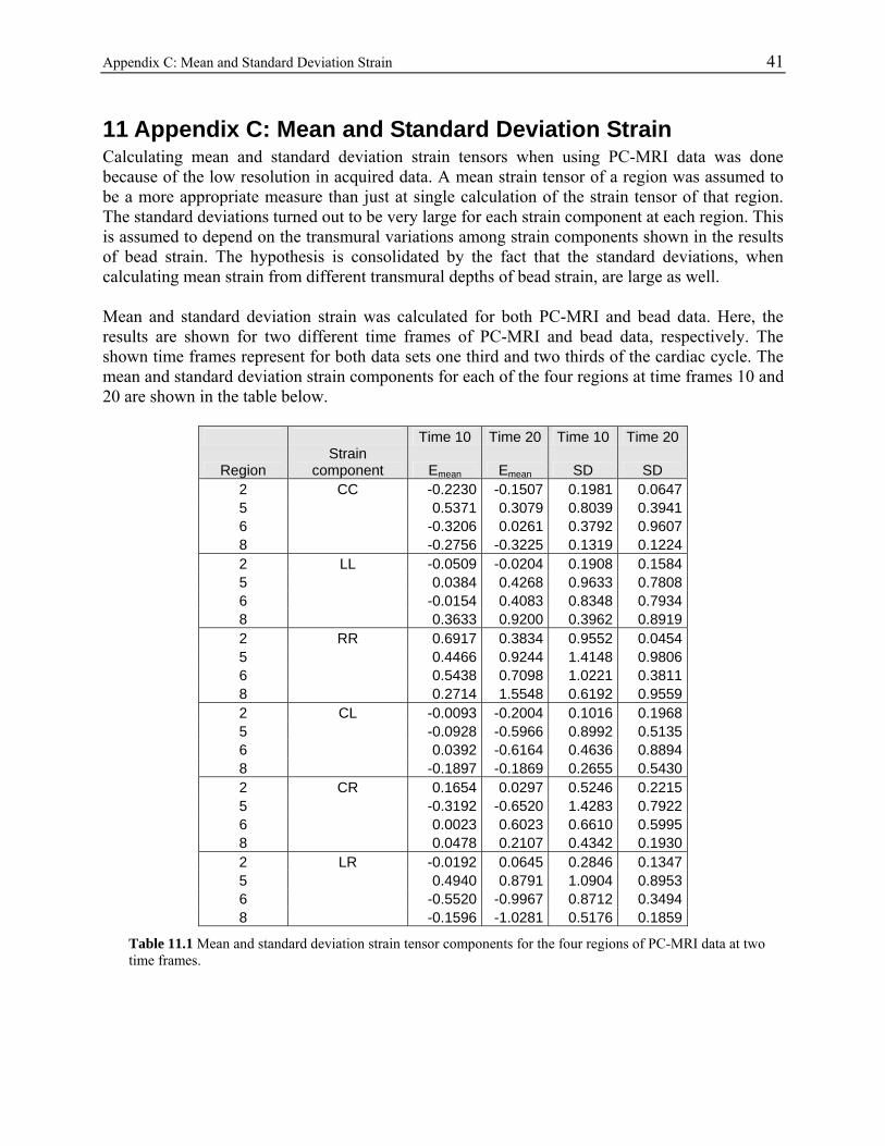
Appendix C: Mean and Standard Deviation Strain 41
11 Appendix C: Mean and Standard Deviation Strain Calculating mean and standard deviation strain tensors when using PC-MRI data was done because of the low resolution in acquired data. A mean strain tensor of a region was assumed to be a more appropriate measure than just at single calculation of the strain tensor of that region. The standard deviations turned out to be very large for each strain component at each region. This is assumed to depend on the transmural variations among strain components shown in the results of bead strain. The hypothesis is consolidated by the fact that the standard deviations, when calculating mean strain from different transmural depths of bead strain, are large as well. Mean and standard deviation strain was calculated for both PC-MRI and bead data. Here, the results are shown for two different time frames of PC-MRI and bead data, respectively. The shown time frames represent for both data sets one third and two thirds of the cardiac cycle. The mean and standard deviation strain components for each of the four regions at time frames 10 and 20 are shown in the table below.
Time 10 Time 20 Time 10 Time 20
Region Strain
component Emean Emean SD SD 2 CC -0.2230 -0.1507 0.1981 0.0647 5 0.5371 0.3079 0.8039 0.3941 6 -0.3206 0.0261 0.3792 0.9607 8 -0.2756 -0.3225 0.1319 0.1224 2 LL -0.0509 -0.0204 0.1908 0.1584 5 0.0384 0.4268 0.9633 0.7808 6 -0.0154 0.4083 0.8348 0.7934 8 0.3633 0.9200 0.3962 0.8919 2 RR 0.6917 0.3834 0.9552 0.0454 5 0.4466 0.9244 1.4148 0.9806 6 0.5438 0.7098 1.0221 0.3811 8 0.2714 1.5548 0.6192 0.9559 2 CL -0.0093 -0.2004 0.1016 0.1968 5 -0.0928 -0.5966 0.8992 0.5135 6 0.0392 -0.6164 0.4636 0.8894 8 -0.1897 -0.1869 0.2655 0.5430 2 CR 0.1654 0.0297 0.5246 0.2215 5 -0.3192 -0.6520 1.4283 0.7922 6 0.0023 0.6023 0.6610 0.5995 8 0.0478 0.2107 0.4342 0.1930 2 LR -0.0192 0.0645 0.2846 0.1347 5 0.4940 0.8791 1.0904 0.8953 6 -0.5520 -0.9967 0.8712 0.3494 8 -0.1596 -1.0281 0.5176 0.1859
Table 11.1 Mean and standard deviation strain tensor components for the four regions of PC-MRI data at two time frames.
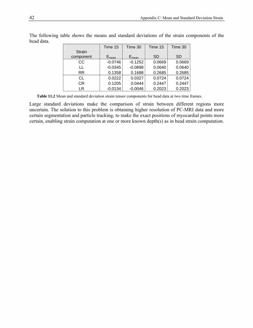
42 Appendix C: Mean and Standard Deviation Strain The following table shows the means and standard deviations of the strain components of the bead data.
Time 15 Time 30 Time 15 Time 30 Strain
component Emean Emean SD SD CC -0.0746 -0.1252 0.0669 0.0669 LL -0.0345 -0.0898 0.0640 0.0640 RR 0.1358 0.1688 0.2685 0.2685 CL 0.0222 0.0327 0.0724 0.0724 CR 0.1205 0.0444 0.2447 0.2447 LR -0.0134 -0.0046 0.2023 0.2023
Table 11.2 Mean and standard deviation strain tensor components for bead data at two time frames.
Large standard deviations make the comparison of strain between different regions more uncertain. The solution to this problem is obtaining higher resolution of PC-MRI data and more certain segmentation and particle tracking, to make the exact positions of myocardial points more certain, enabling strain computation at one or more known depth(s) as in bead strain computation.
References 43
12 References Aletras A, Ding S, Balaban R, Wen H (1999). DENSE: Displacement Encoding with Stimulated Echoes in Cardiac Functional MRI. Journal of Magnetic Resonance, 137: 247-252 Arts T, Costa KD, Covell JW, McCulloch AD (2001). Relating Myocardial Laminar Architecture to Shear Strain and Muscle Fiber Orientation. American Journal of Physiology, Heart and Circulatory Physiology, 280: H2222-H2229 Bogaert J, Rademakers F (2001). Regional Nonuniformity of Normal Adult Human Left Ventricle. American Journal of Physiology, Heart and Circulatory Physiology, 280: H610-H620 Boring, E (1998). Visualization of tensor fields, Master Thesis, University of California, Santa Cruz Bowen, RM (1989). Introduction to Continuum Mechanics for Engineers. Plenum Press, New York, ISBN: 0-306-43050-9 Brandt Heiberg E (2001). Automated Feature Detection in Multidimensional Images – a unified tensor approach. Linköpings universitet, Linköping Studies in Science and Technology Thesis No. 909, ISBN: 91-7373-131-5 Escobar Kvitting J-P, Ebbers T, Engvall J, Sutherland GR, Wranne B, Wigström L (2000). Three-directional Myocarcardial Motion Assessed Using 3D Phase Contrast MRI. Presented in part at the ESMRMB 17th annual meeting, Paris, September 2000 Fung YC (1969). A first course in continuum mechanics. Prentice-Hall, ISBN: 13-171637-9 Humphrey JD (2002). Cardiovascular Solid Mechanics, Cells Tissues and Organs. Springer Verlag, New York, ISBN: 0-387-95168-7 Karlsson M, Glasson J, Bolger A, Daughters G, Komeda M, Foppiano L, Miller C, Ingels N (1998). Mitral Valve Opening in the Ovine Heart. American Journal of Physiology, Heart and Circulatory Physiology, 274: H552-563 McCulloch AD (1995). Cardiac Biomechanics. In: The Biomedical Engineering Handbook. (Bronzino JD, ed), CRC Press, Boca Raton, pp 418-439. Meier G, Bove A, Santamore W, Lynch P (1980). Contractile Function in Canine Right Ventricle. American Journal of Physiology, Heart and Circulatory Physiology, 239(6): H794-H804 Råde L, Westergren B (1998). Mathematics Handbook for Science and Engineering. Studentlitteratur, Lund, ISBN: 91-44-00839-2
44 References Selskog P, Brandt Heiberg E, Ebbers T, Wigström L, Karlsson M (2002a). Kinematics of the Heart: Strain Rate Imaging from Time-Resolved Three-Dimensional Phase Contrast MRI. IEEE Transactions on Medical Imaging, 21(9): 1105-1109 Selskog P, Torstenfelt B, Ebbers T, Wigström L, Karlsson M (2002b). Kinematics of the Heart – Finite Elements and 3D Time-Resolved Phase-Contrast Magnetic Resonance Imaging. Proceedings of 9th FEM Workshop at University of Ulm, Germany, July, 2002 Tortora G, Grabowski SR (2000). Principles of Anatomy and Physiology. John Wiley & Sons Inc, New York, ISBN: 0-471-36692-7 Tseng W-YI, Reese TG, Weisskoff RM, Brady TJ, Wedeen VJ (2000). Myocardial Fiber Shortening in Humans: Initial Results of MR Imaging. Radiology, 216: 128-139 Waldman L, Fung YC, Cowell JW (1985). Transmural Myocardial Deformation in the Canine Left Ventricle. Circulation Research, 57: 152-163 Wigström L, Sjöqvist L, Wranne B (1996). Temporally Resolved 3D Phase-Contrast Imaging. Magnetic Resonance in Medicine, 36: 800-803 Wigström L (2003). Multidimensional Magnetic Resonance Imaging. Linköpings Universitet, Linköping Studies in Science and Technology Dissertations No. 807, ISBN 91-7373-616-3 Zhu Y, Drangova M, Pelc NJ (1996). Fourier Tracking of Myocardial Motion Using Cine-PC Data. Magnetic Resonance in Medicine, 35: 471-480


![KINEMATICS - new.excellencia.co.innew.excellencia.co.in/college/web/pdf/Kinematics-merged.pdf · KINEMATICS KINEMATICS WORKSHEET 1 1) Displacement is a _____ [ ] 1) Vector quantity](https://img.pdfslide.us/doc/110x75/5f356d4687229051801abace/kinematics-new-kinematics-kinematics-worksheet-1-1-displacement-is-a-.jpg)