Regional fluxes of methane in the Surat Basin, Queensland

Regional fluxes of methane in the Surat Basin, QueenslandStakeholder Roundtable Group meeting

David Etheridge | Principal Research Scientist, Climate Science CentreCSIRO Oceans and Atmosphere Aspendale, Victoria

4 November 2019

2GISERA Stakeholder Roundtable 4 November 2019

GISERA Stakeholder Roundtable 4 November 2019 3

Aim of the project

• Demonstrate the utility of an atmospheric “top-down” or inverse modelling approach to infer regional scale (~ 100 – 1000 km) methane emissions across the Surat Basin

• Monitoring from 2 stations: Ironbark and Burncluith (concurrent measurements during July 2015 – December 2016)

• Compare with “bottom-up” inventory emissions


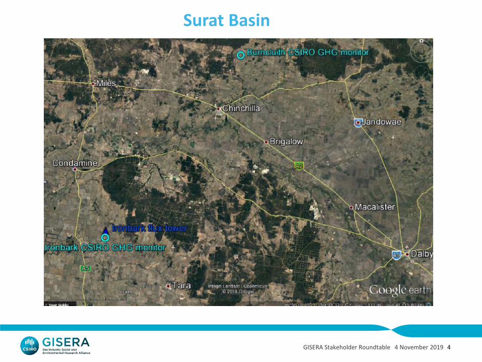
Surat Basin

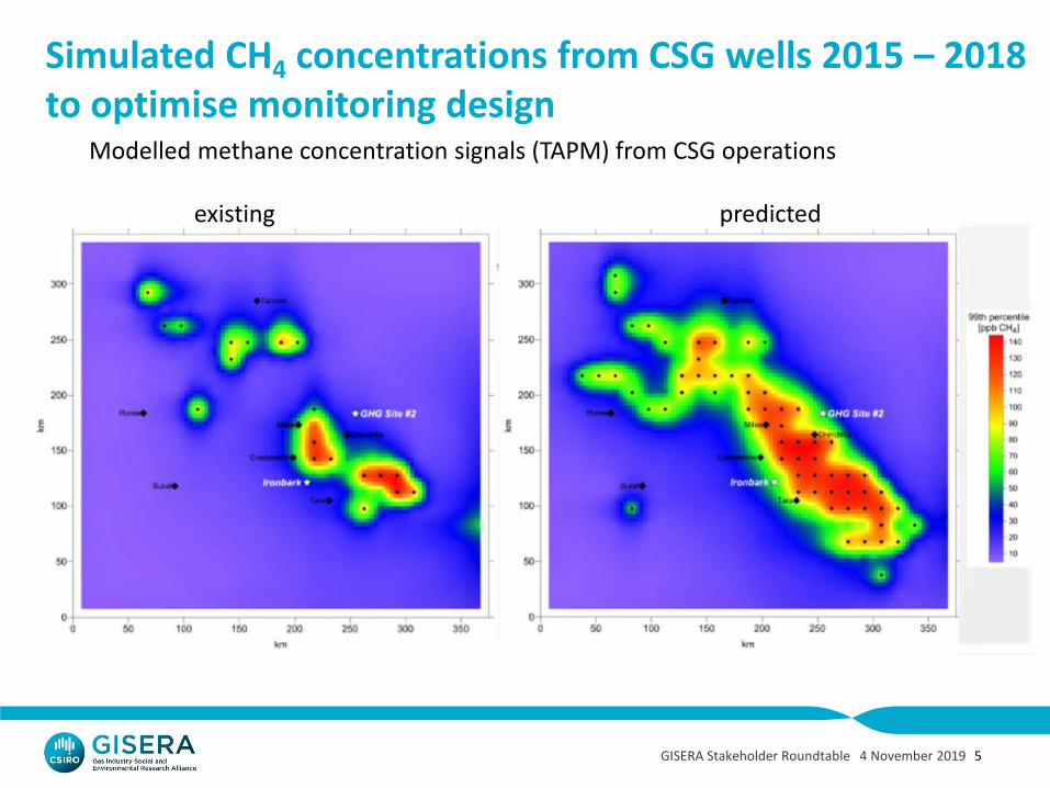
Simulated CH4 concentrations from CSG wells 2015 – 2018to optimise monitoring design

Modelled methane concentration signals (TAPM) from CSG operations

existing predicted


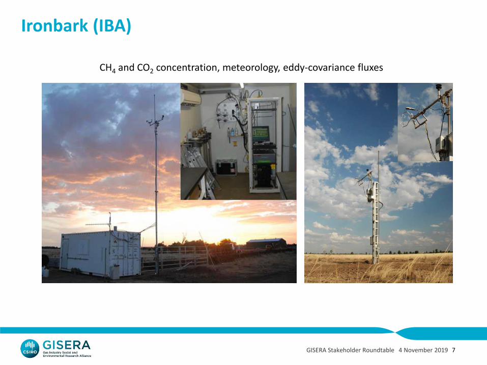
Ironbark (IBA)

CH4 and CO2 concentration, meteorology, eddy-covariance fluxes


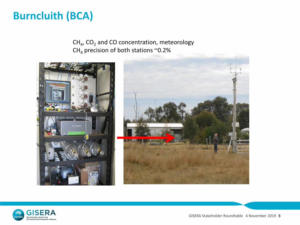
Burncluith (BCA)

CH4, CO2 and CO concentration, meteorologyCH4 precision of both stations ~0.2%


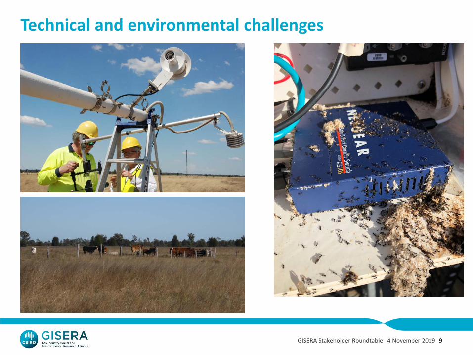
Technical and environmental challenges


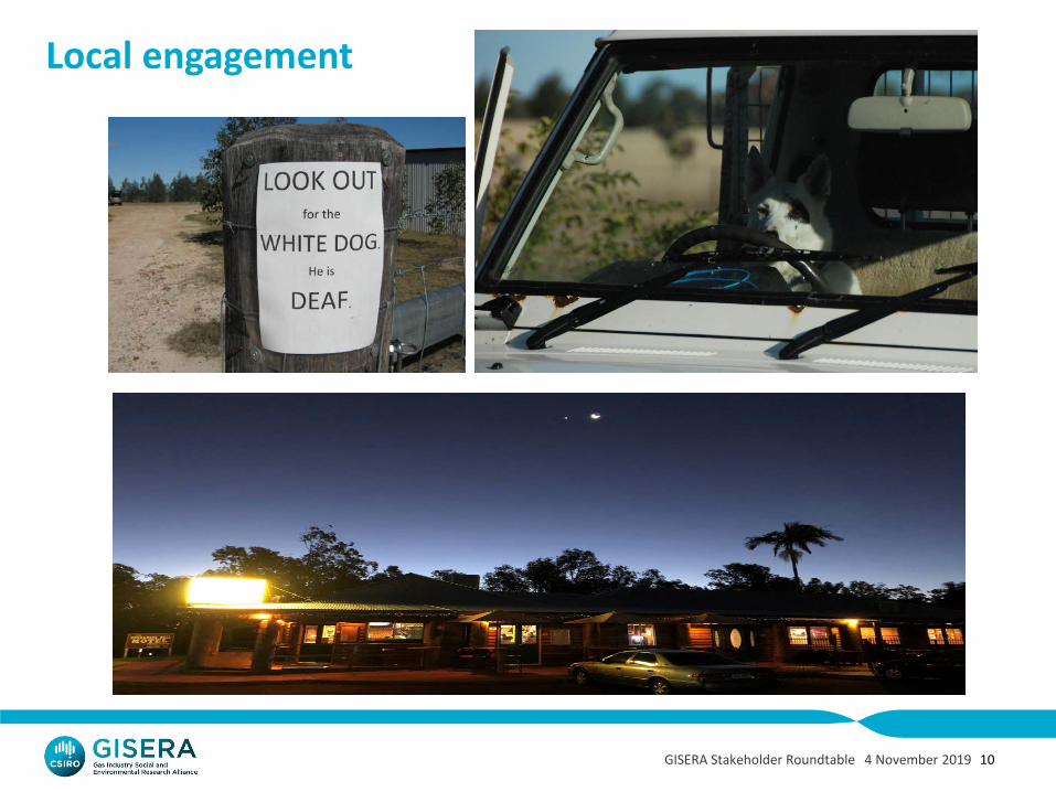
Local engagement


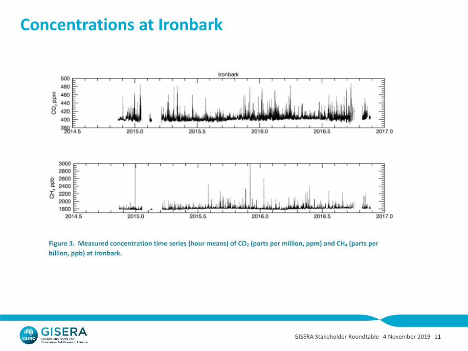
Concentrations at Ironbark


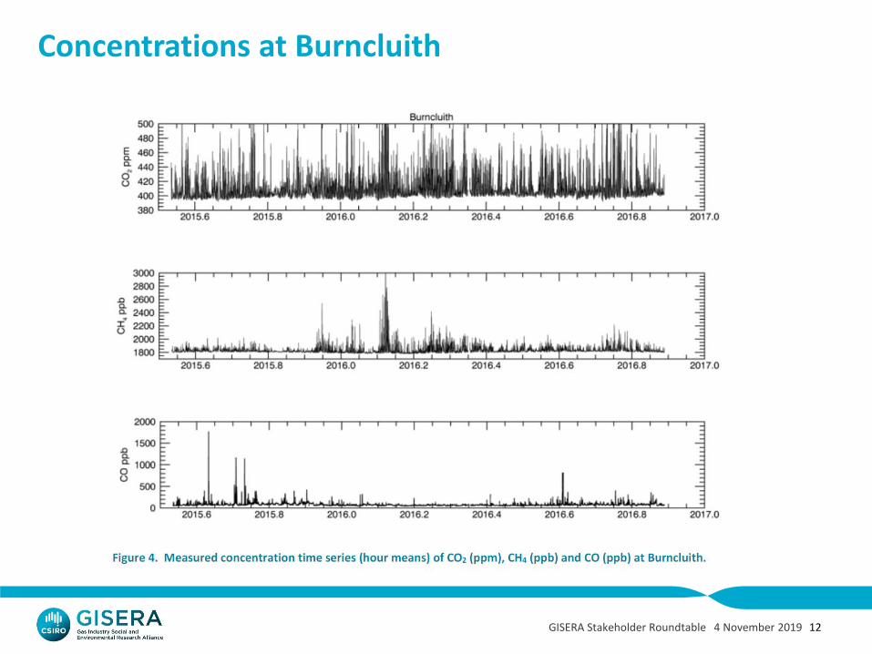
Concentrations at Burncluith


Data selection and filtering


Removal of unwanted signals • Cows near analyser inlets (detected by CO2)• Burning off and dwelling open fire (CO)• Nocturnal data (high stability, low wind speeds, extreme concentration gradients)

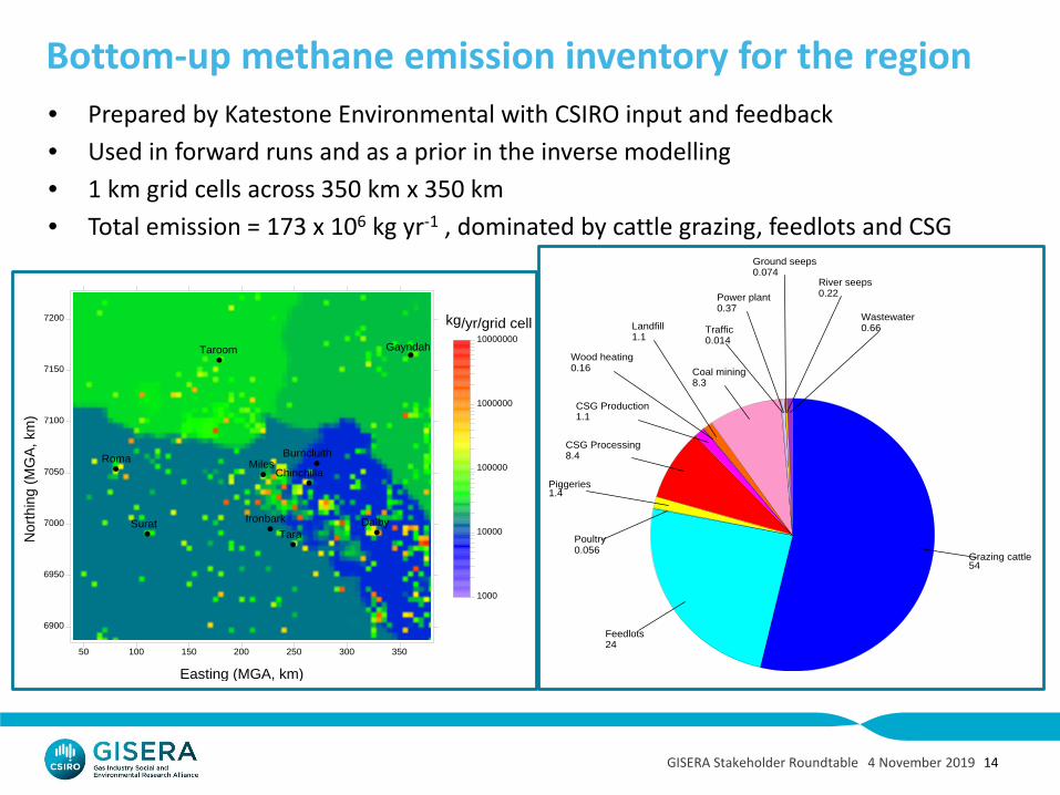
Bottom-up methane emission inventory for the region • Prepared by Katestone Environmental with CSIRO input and feedback • Used in forward runs and as a prior in the inverse modelling• 1 km grid cells across 350 km x 350 km• Total emission = 173 x 106 kg yr-1 , dominated by cattle grazing, feedlots and CSG

Grazing cattle54

Feedlots24

Poultry0.056

Piggeries1.4

CSG Processing8.4

CSG Production1.1

Wood heating0.16

Landfill1.1

Coal mining8.3

Traffic0.014

Power plant0.37

Ground seeps0.074

River seeps0.22

Wastewater0.66

50 100 150 200 250 300 350

Easting (MGA, km)

6900

6950

7000

7050

7100

7150

7200

Nor

thin

g (M

GA,

km

)

Ironbark

BurncluithMiles

Chinchilla

Gayndah

Dalby

Roma

SuratTara

Taroom

1000

10000

100000

1000000

10000000

kg/yr/grid cell


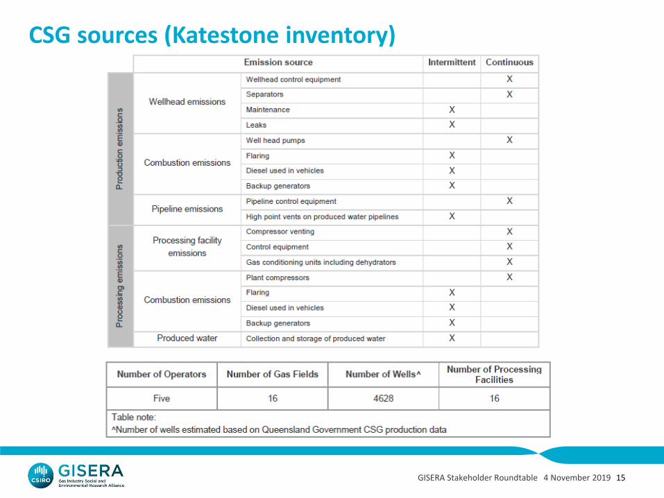
CSG sources (Katestone inventory)



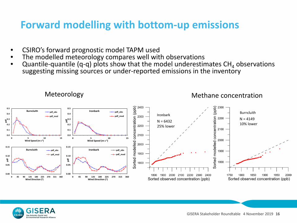
• CSIRO’s forward prognostic model TAPM used• The modelled meteorology compares well with observations• Quantile-quantile (q-q) plots show that the model underestimates CH4 observations

suggesting missing sources or under-reported emissions in the inventory

Methane concentration

Forward modelling with bottom-up emissions

0.0

0.1

0.2

0.3

0.4

0.5

0 5 10 15

pdf

Wind Speed (m s-1)

Burncluith pdf_obs

pdf_mod

0.0

0.1

0.2

0.3

0.4

0.5

0 5 10 15

pdf

Wind Speed (m s-1)

Ironbark pdf_obs

pdf_mod

0.00

0.05

0.10

0.15

0 45 90 135 180 225 270 315 360

pdf

Wind Direction (o)

Burncluith pdf_obs

pdf_mod

0.00

0.05

0.10

0.15

0 45 90 135 180 225 270 315 360

pdf

Wind Direction (o)

Ironbark pdf_obs

pdf_mod

Meteorology

N = 643225% lower

N = 414910% lower

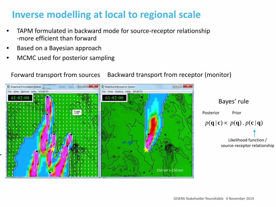
Inverse modelling at local to regional scale

● OCEANS AND ATMOSPHERE

• TAPM formulated in backward mode for source-receptor relationship -more efficient than forward

• Based on a Bayesian approach • MCMC used for posterior sampling

( | ) ( ) . ( | )p p p∝q c q c q

Bayes’ rule Posterior Prior

Likelihood function /source-receptor relationship

250 km x 250 km

Forward transport from sources Backward transport from receptor (monitor)

GISERA Stakeholder Roundtable 4 November 201917 |

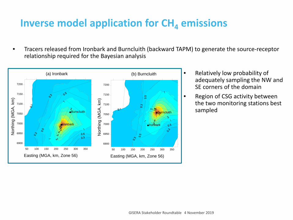
• Tracers released from Ironbark and Burncluith (backward TAPM) to generate the source-receptor relationship required for the Bayesian analysis

Inverse model application for CH4 emissions

50 100 150 200 250 300 350

Easting (MGA, km, Zone 56)

6900

6950

7000

7050

7100

7150

7200

Nor

thin

g (M

GA,

km

)

Ironbark

Burncluith

(a) Ironbark (b) Burncluith

50 100 150 200 250 300 350

Easting (MGA, km, Zone 56)

6900

6950

7000

7050

7100

7150

7200

Nor

thin

g (M

GA,

km

)

Ironbark

Burncluith

• Relatively low probability of adequately sampling the NW and SE corners of the domain

• Region of CSG activity between the two monitoring stations best sampled



• 11 x 11 source regions considered (31 x 31 km)• July 2015-December 2016• Model and background methane uncertainties were accounted for• Three cases of emission prior specified

1) Loose bounds (10-10,000 g s-1 per source area) – uninformative prior2) Spatially uniform prior (45.4 g s-1 per source area), Gaussian uncertainty of 10%3) Bottom up inventory as prior, Gaussian uncertainty of 3%

Simulation details

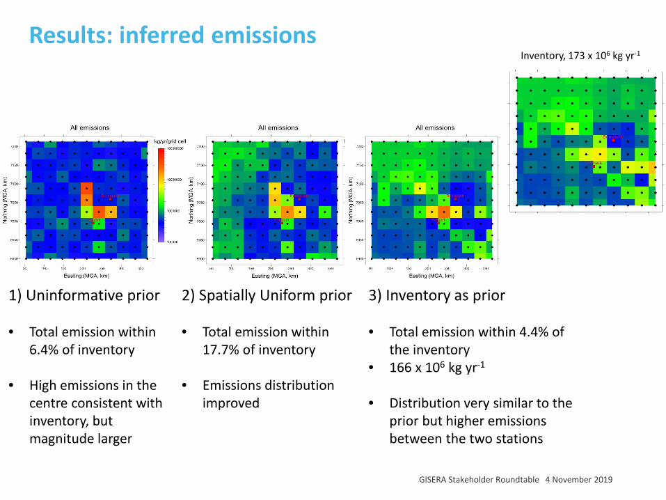
Results: inferred emissionsInventory, 173 x 106 kg yr-1

1) Uninformative prior

• Total emission within 6.4% of inventory

• High emissions in the centre consistent with inventory, but magnitude larger

3) Inventory as prior

• Total emission within 4.4% of the inventory

• 166 x 106 kg yr-1

• Distribution very similar to the prior but higher emissions between the two stations

2) Spatially Uniform prior

• Total emission within 17.7% of inventory

• Emissions distribution improved


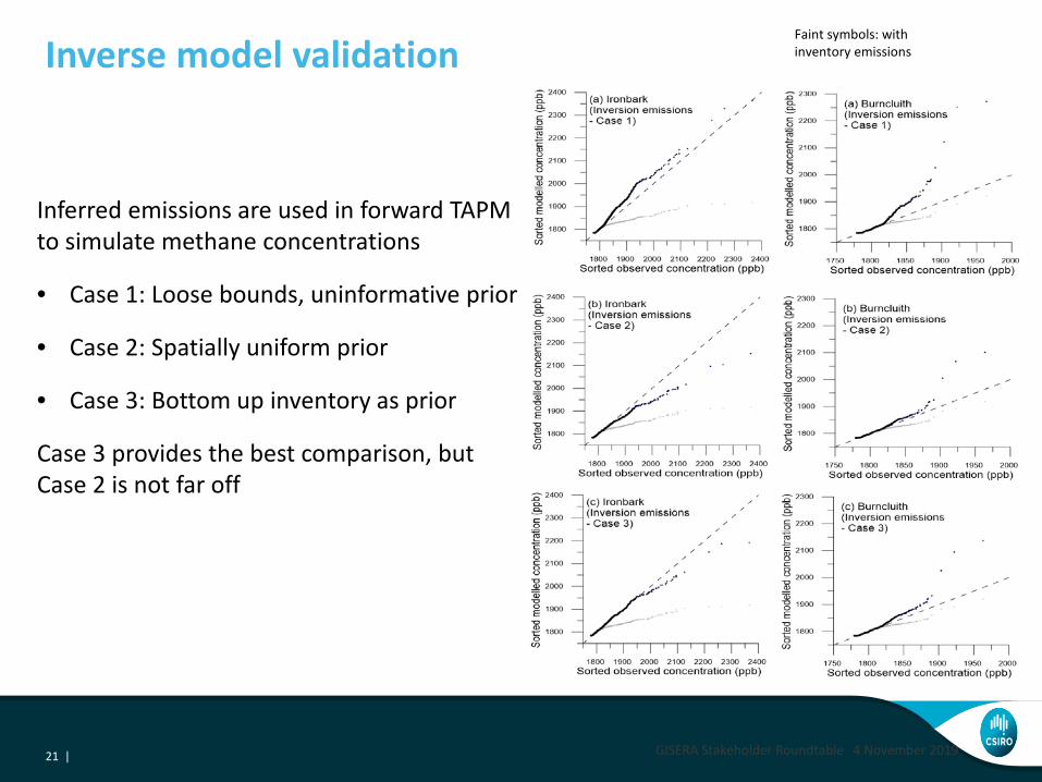
Inverse model validation

Inferred emissions are used in forward TAPM to simulate methane concentrations

• Case 1: Loose bounds, uninformative prior

• Case 2: Spatially uniform prior

• Case 3: Bottom up inventory as prior

Case 3 provides the best comparison, but Case 2 is not far off

Faint symbols: with inventory emissions


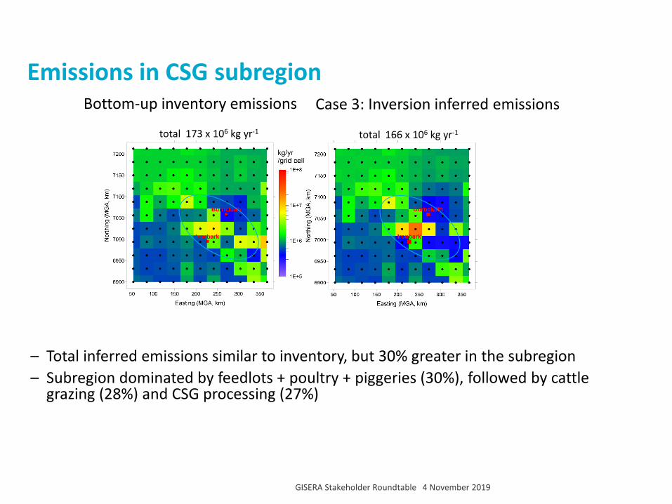
Emissions in CSG subregion

– Total inferred emissions similar to inventory, but 30% greater in the subregion– Subregion dominated by feedlots + poultry + piggeries (30%), followed by cattle

grazing (28%) and CSG processing (27%)

Bottom-up inventory emissions Case 3: Inversion inferred emissions

total 173 x 106 kg yr-1 total 166 x 106 kg yr-1


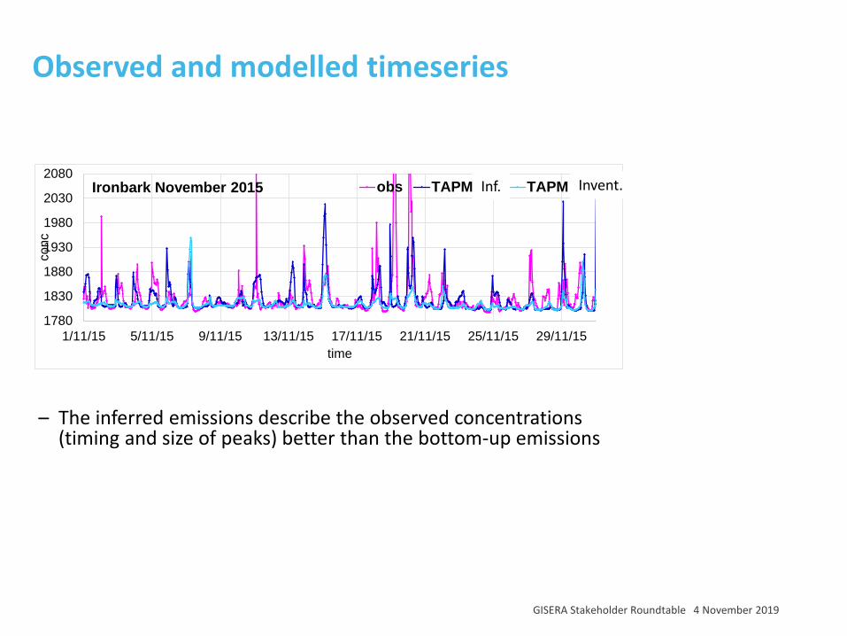
Observed and modelled timeseries

1780

1830

1880

1930

1980

2030

2080

1/11/15 5/11/15 9/11/15 13/11/15 17/11/15 21/11/15 25/11/15 29/11/15

conc

time

Ironbark November 2015 obs TAPM inv TAPM ori

– The inferred emissions describe the observed concentrations (timing and size of peaks) better than the bottom-up emissions

Invent.Inf.



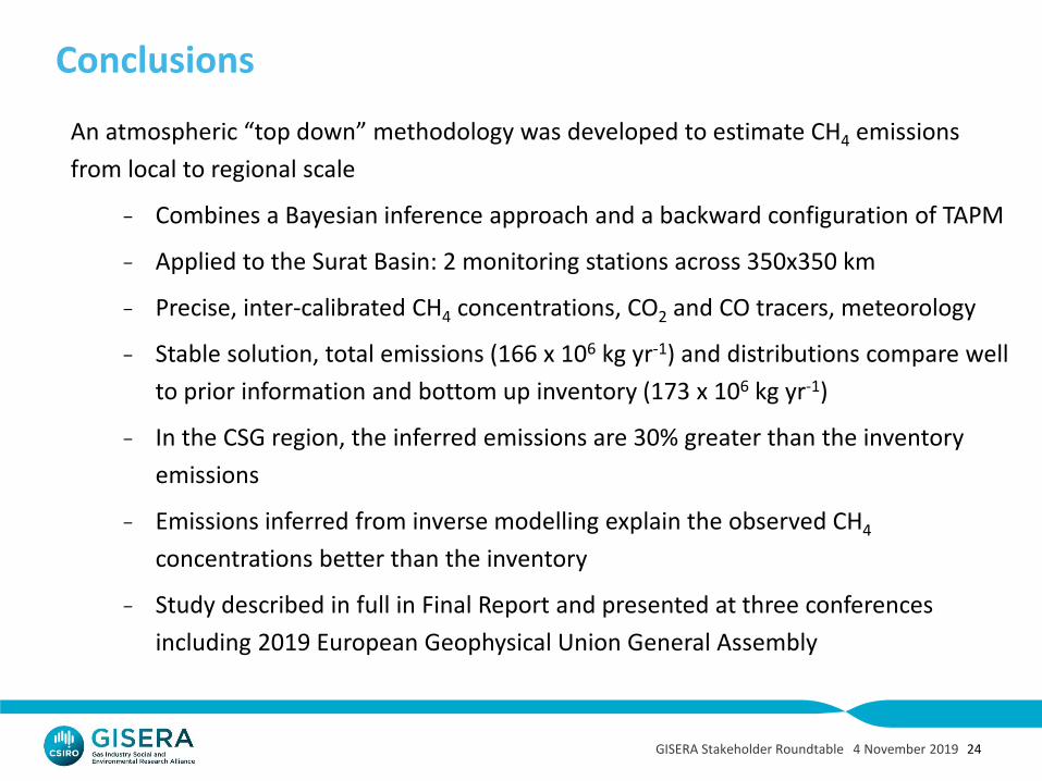
Conclusions

An atmospheric “top down” methodology was developed to estimate CH4 emissions from local to regional scale

– Combines a Bayesian inference approach and a backward configuration of TAPM

– Applied to the Surat Basin: 2 monitoring stations across 350x350 km

– Precise, inter-calibrated CH4 concentrations, CO2 and CO tracers, meteorology

– Stable solution, total emissions (166 x 106 kg yr-1) and distributions compare well to prior information and bottom up inventory (173 x 106 kg yr-1)

– In the CSG region, the inferred emissions are 30% greater than the inventory emissions

– Emissions inferred from inverse modelling explain the observed CH4

concentrations better than the inventory

– Study described in full in Final Report and presented at three conferences including 2019 European Geophysical Union General Assembly


Further work

– Journal publication

– Explore value in other data – moving platforms (aircraft, vehicles), small low cost sensors, satellites

– Additional tracers to quantify source types – CH4 isotopes, accompanying gases

– Follow up studies (after future growth and eventual wind down in CSG activity)

– Zone in on “hot spots” indicated by inversion

Acknowledgements

• CSIRO’s Gas Industry Social and Environmental Research Alliance (GISERA)

Research reports https://gisera.csiro.au/project/methane-seepage-in-the-surat-basin

• CSIRO Oceans and Atmosphere (GASLAB), Energy, Land and Water, AIM Future Science Platform

• Katestone Environmental Pty Ltd (Natalie Shaw, Lisa Smith, Tania Haigh, Michael Burchill)

• CSG companies for activity data

• CSIRO Internal Reviewers (Mark Hibberd and Martin Cope)

• Land owners (G. and S. McConnachie; Origin Energy)


https://gisera.csiro.au/project/methane-seepage-in-the-surat-basin

Thank you

David EtheridgePrincipal Research Scientist

t +61 3 9239 4590e [email protected] gisera.csiro.au

https://research.csiro.au/acc/

Ashok LuharPrincipal Research Scientist

t +61 3 9239 4624e [email protected] gisera.csiro.au

Documents

Regional fluxes of methane in the Surat Basin, Queensland