REGION 4

ANNUAL SUMMARY REPORT

2001 – 2004

EFFECTIVENESS MONITORING PROGRAM

FOR

STREAMS AND RIPARIAN AREAS WITHIN THE

UPPER COLUMBIA RIVER BASIN

PREPARED BY:

PIBO EFFECTIVENESS MONITORING PROGRAM STAFF

SUMMARY REPORT

2001–2004

EFFECTIVENESS MONITORING PROGRAM

FOR

STREAMS AND RIPARIAN AREAS WITHIN THE

UPPER COLUMBIA RIVER BASIN

REGION R4

PREPARED BY:

Dax Dugaw

Jeremiah Heitke

Greg Kliewer

Boyd Bouwes

PIBO EFFECTIVENESS MONITORING PROGRAM STAFF

ACKNOWLEDGEMENTS

We wish to thank the many people who supported our work throughout the year. First, we would like to thank the Regional Deputy Team in Regions 1, 4, and 6 of the Forest Service, and the Idaho and Oregon/Washington BLM for funding the program. We appreciate the guidance, energy, and input provided by Tim Burton, Gina Lampman, and other members of the IIT Monitoring Task Team.

We would like to thank the supervisors and sampling crews who are the backbone of the program. In particular, we thank the crews from the 2004 field season.

2004 Field Supervisors were: Alex Anderson, Alison Berry, Tony Burrows, Ryan Colyer, Dax Dugaw, Andy Hill, Ali Kelly, Heath Whitacre, Jeremiah Heitke, and Boyd Bouwes.

Crew Members were: Luca Adelfio, Jade Alicandro, Erik Archer, Sherry Adams, Missy Barnes, Anne Birnie, Sarah Brandy, Keyna Bugner, Zacchaeus Compson, Greg Huchko, Sarah Klingsporn, Kirk Lambrecht, Ryan Leary, Jeff LeBrun, Tyler Logan, Kipp Marzullo, Jamie McEvoy, Diane Menuz, Kate Metzger, Ralph Mitchell, Ariel Muldoon, Matt Peters, Sarah Quistberg, Tyler Ramaker, Jacob Riley, Sabrina Rust, Ryan Salem, Jacob Schaub, Paul Schwartz, Kyle Steele, Holly Truemper, Julia Vinciguerra, Richard Wathen, Nicholas Weber, Stewart Wechsler, Kevin Weinner, and Benjamin Wright.

A special thanks to the linchpin of the PIBO program, Greg Kliewer, for managing our complex and ever growing database.

We received invaluable support from a large number of Forest Service and BLM personnel at Forest and District Offices throughout the study area. We cannot list each individual separately, but would like to thank all of you.

We appreciate the help and support from other large scale monitoring groups. Gretchen Hayslip, Bob Hughes, Philip Kaufmann, Phil Larsen, and Tony Olsen from the EPA EMAP project have been extremely helpful in addressing study design and data analysis issues; Kirsten Gallo, Steve Lanigan, and Chris Moyer from the NWFP AREMP effort; Doug Drake, Rick Hafele, and Shannon Hubler from Oregon DEQ; and Chris Mebane from Idaho DEQ.

In addition, Michele Bills, Sheryl Ware, Pat Wicks, and Patty Ybright-Jessop continue to go above and beyond the call of duty providing logistic and administrative support to keep the program running smoothly. We thank Dave Turner for directing our statistical analyses and Deanna Vinson for editing manuscripts and managing the budget. As always, thanks to the personnel from the BLM/USU National Aquatic Monitoring Center for identifying and reporting the invertebrate identifications. A special thanks to Chuck Hawkins and Yong Cao for developing a RIVPACS model for our invertebrate data.

i

ABSTRACT

The primary objective of this program is to answer the question: “Are key biological and physical components of aquatic and riparian communities improved, degraded, or restored in the range of steelhead and bull trout?” The study area covers the portion of the Columbia River Basin with Forest Service lands designated within INFISH and PACFISH, and BLM lands within PACFISH or containing bull trout. We conducted a pilot study from 1998 through 2000 and concluded that the approach was logistically feasible, successfully measured reach conditions, and provided an effective foundation to guide future sampling efforts. In 2001, we began the first 5 year sampling cycle with the program at half implementation. Approximately 150 sub-watersheds were sampled in both 2001 and 2002. At full implementation (which began in 2003), we sample 250 sub-watersheds per year or 1250 every 5 years. An additional 50 sub-watersheds (sentinel reaches) are sampled annually. In 2006, we will begin sampling reaches that were originally sampled in 2001. At this time, we will begin addressing our objective of assessing change in resource conditions given current land management practices.

This report summarizes the information collected from 2001 through 2004. The program has sampled reaches within 20 National Forests, five Oregon/ Washington BLM Districts, and three Idaho BLM Districts. A total of 783 sub-watersheds have been sampled including 288 in Region 1, 232 in Region 4, 183 in Region 6, 44 in Idaho BLM, and 36 in OR/WA BLM. Fifty of these reaches are considered “sentinel” reaches and are sampled annually. One hundred and fifty reaches (19%) were in reference sub-watersheds and 626 were in managed sub-watersheds. In addition, the program sampled 211 grazing designated monitoring areas (DMA) reaches.

The report includes an overview of the sampling design, description of methods, and summarized data for each BLM State Office, BLM District, FS Region, and National Forest. Box and whisker plots show the distribution of each variable for both managed and reference sub-watersheds. Additional data summaries, analyses, and interpretation are presented in peer reviewed publications. The appendices include data definitions and descriptions of summary variables, summary tables, reach description page(s) from 2004, and a sample reach photo page. Finally, we have included a CD containing this report, the Effectiveness Monitoring Plan and sampling protocols, publications, presentations, and summary data for all reaches sampled since 2001. The CD also contains photo pages, reach maps, and topographic maps for all 2003 and 2004 reaches.

ii

CONTENTS INTRODUCTION............................................................................................. 1

Study Area................................................................................................... 3 Sample Reach Selection and Description.................................................... 4 Data Collection .......................................................................................... 11 Quality Assurance Program....................................................................... 18

SUMMARIZED DATA ................................................................................... 18 Reach Summary Graphs ........................................................................... 20

SPECIAL PROJECTS................................................................................... 29 PUBLICATIONS............................................................................................ 29 REFERENCES.............................................................................................. 32 APPENDIX A - DEFINITIONS AND DESCRIPTIONS OF SUMMARY VARIABLES .................................................................................................. 36 APPENDIX B – REACH SUMMARY TABLES .............................................. 44 APPENDIX C – REACH DESCRIPTION(S) AND PHOTO PAGE................. 45

iii

INTRODUCTION

The decline of the steelhead trout (Onchorynchus mykiss gairdneri) and bull trout (Salvelinus confluentus) in the upper Columbia River Basin has prompted interest in the current condition of habitat throughout the range of these species. In particular, the effect of forest management activities on spawning and rearing habitat is under increased scrutiny. Forest management activities such as timber harvest, road construction, and livestock grazing have all been shown to negatively influence stream habitat. However, recent large-scale conservation strategies may protect habitat and promote recovery of degraded habitat throughout the range.

There are several documents that provide guidance for protecting anadromous fish habitat in the Columbia River Basin. Each National Forest within the range of steelhead trout in the Columbia River Basin has completed a forest plan that guides the protection and management of aquatic and riparian resources on the forest (USDA NFMA 1976). Due to increased concern over the status of anadromous salmonids, the United States Department of Agriculture (USDA) Forest Service (USFS) and United States Department of Interior (USDI) Bureau of Land Management (BLM) developed an aquatic and riparian area management strategy to protect habitat for Pacific anadromous salmonids (PACFISH 1994). The purpose of this strategy was to provide consistent, interim guidance to National Forests, and to develop interim management objectives for fish habitat prior to the revision of forest plans. The Interior Columbia Basin Ecosystem Management Plan (ICBEMP) was developed to provide a long-term strategy to manage resources within the Columbia River Basin. As part of this plan, aquatic and riparian management guidelines were developed that would replace the more general guidance of PACFISH and provide direction for the restoration of habitats throughout the basin.

The recent listing of steelhead and bull trout under the Endangered Species Act prompted a review of current habitat management practices on federal lands by the United States Department of Commerce, National Marine Fisheries Service (NMFS), and USDI, Fish and Wildlife Service (USFWS). As part of the Section 7 consultation process with the BLM and USFS, the NMFS and USFWS issued Biological Opinions on the adequacy of land and resource plans to protect anadromous fish habitat. One of the commitments identified in the Biological Opinions was to monitor managed lands, specifically those grazed by livestock, to determine if current management practices were meeting PACFISH riparian management objectives.

The interagency effectiveness monitoring team (USFS, BLM, NMFS, and USFWS) convened in April 1998 to develop a plan for monitoring the condition of steelhead and bull trout habitat in grazed lands (Kershner et al. 2004a). The team developed a draft monitoring plan in May 1998. The team has met annually since then to update the draft, using information from the previous sampling efforts and peer reviews of the plan. In 2001, the effort was expanded from sampling on grazed and unmanaged lands only, to include all managed lands within the study area. Goals for this plan (from the Biological Opinions) include developing a coordinated effort with a defensible sample design, maximizing the effectiveness of limited monitoring funds, identifying appropriate scales and levels of monitoring, and

1

identifying how monitoring results should be used to make management adjustments. The group recognized that a variety of management activities affect aquatic and riparian systems and effects from one or more activities can be cumulative. An approach to monitoring that considers these relationships and attempts to track their effects will ultimately provide the kind of feedback needed to adapt specific management activities on federal lands.

At the request of USFS Region 4, the USFS National Fish and Aquatic Ecology Unit conducted pilot efforts in 1998 and 1999 within the Salmon River drainage of central Idaho. Since 2000, we have expanded the study area and now sample throughout the upper Columbia River Basin in USFS Regions 1, 4, and 6 and BLM lands within PACFISH or containing bull trout. The primary goal was to determine the feasibility of an extensive approach to address the following question: Are key biological, chemical, and physical attributes, processes, and functions of riparian and aquatic systems degraded, maintained, or restored in the range of the steelhead and bull trout as a result of land management within the upper Columbia River Basin (Kershner et al. 2004a). We defined the effectiveness monitoring component of this program with the following three objectives:

1) Determine whether key biological and physical attributes, processes, and

functions of upland, riparian, and aquatic systems are being degraded, maintained, or restored across the PACFISH/INFISH Biological Opinion Effectiveness Monitoring Program (PIBO-EMP) study area.

2) a) Determine the direction and rate of change in riparian and aquatic habitats over time as a function of management practices. b) Determine whether riparian and aquatic habitat conditions at integrator reaches are reflective of conditions throughout the watershed.

3) Determine whether specific Key Management Practices (KMPs) for livestock grazing are effective in maintaining or restoring riparian structure and function.

2

METHODS Study Area

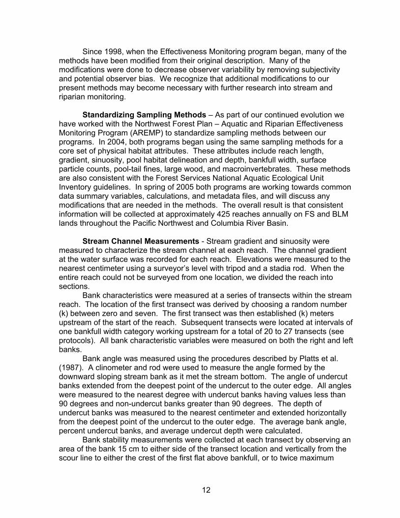
The study area includes portions of eastern Oregon and Washington, Idaho,

and western Montana (Figure 1). It is bordered by the Cascade Mountains on the west, Canada to the north, the continental divide on the east from Canada south to the Beaverhead Mountains, and the headwaters of the Snake, John Day, and Deschutes Rivers to the south. The Snake River Basin upstream of American Falls, Idaho was excluded. The study area includes major spawning areas for steelhead and bull trout, as well as chinook (Oncorhynchus tshawytscha) and sockeye salmon (Oncorhynchus nerka), which are also listed.

The lands within the study area are highly diverse and include the high mountains in central Idaho and western Montana, basalt plateaus in eastern Oregon and Washington, and high desert in southern Idaho. The landscape has been heavily influenced by continental ice sheets, mountain glaciers, and several cataclysmic floods (Quigley and Arbelbide 1997). Elevations range from less than 500 m along the lower Columbia River to over 3000 m in the mountains.

Precipitation in the study area predominately falls as snow from October to May (Quigley and Arbelbide 1997). Some precipitation falls as rain during the spring, summer, and fall months. Temperatures within the study area are highly variable with short, cool summers in the mountainous areas and longer, extended growing seasons in the montane valleys and lower elevations. Winters are typically cold with sub-freezing temperatures from mid-November to April being the norm.

Valley bottom types are characterized as steep confined valleys, moderately steep/moderately confined valleys, and flat moderately confined valleys (Quigley and Arbelbide 1997). Streams within grazed systems represent a full variety of stream types from steep, confined streams to highly braided, meandering meadow streams.

Forest vegetation within the study area is dominated by dry forests (douglas fir, ponderosa pine, grand fir, white fir) and cold forest (mountain hemlock, spruce-fir, aspen, white bark pine, lodgepole pine, alpine larch). Range vegetation groups include dry grass (fescue, wheatgrass), dry shrub (bitterbrush, sagebrush, juniper), cool shrub (mountain big sage, mountain shrub), riparian shrub (willows), riparian herb (sedges), and riparian woodlands (cottonwood, aspen) (Quigley and Arbelbide 1997).

Livestock grazing has occurred in the study area since the late 19th century. Range integrity ratings are low-moderate throughout most of the study area (Quigley and Arbelbide 1997).

3

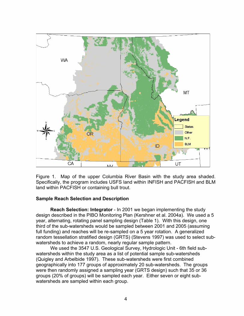
Figure 1. Map of the upper Columbia River Basin with the study area shaded. Specifically, the program includes USFS land within INFISH and PACFISH and BLM land within PACFISH or containing bull trout.

Sample Reach Selection and Description

Reach Selection: Integrator - In 2001 we began implementing the study

design described in the PIBO Monitoring Plan (Kershner et al. 2004a). We used a 5 year, alternating, rotating panel sampling design (Table 1). With this design, one third of the sub-watersheds would be sampled between 2001 and 2005 (assuming full funding) and reaches will be re-sampled on a 5 year rotation. A generalized random tessellation stratified design (GRTS) (Stevens 1997) was used to select sub-watersheds to achieve a random, nearly regular sample pattern.

We used the 3547 U.S. Geological Survey, Hydrologic Unit - 6th field sub-watersheds within the study area as a list of potential sample sub-watersheds (Quigley and Arbelbide 1997). These sub-watersheds were first combined geographically into 177 groups of approximately 20 sub-watersheds. The groups were then randomly assigned a sampling year (GRTS design) such that 35 or 36 groups (20% of groups) will be sampled each year. Either seven or eight sub-watersheds are sampled within each group.

4

Within each group, a sub-watershed must meet two criteria in order to be sampled. First, it must contain a “response” reach with a gradient less than 3%. This reach type was chosen because it displays the greatest response to upstream impacts from management activities (Montgomery and McDonald 2002). Secondly, the watershed upstream of the sample reach must contain greater than 50% FS / BLM ownership. Sub-watersheds that meet these two criteria were then stratified as “managed” or “reference”. Sub-watersheds were categorized as “reference” if: 1) they were not grazed by livestock within the last 30 years, 2) road densities were less than 0.5km / km2, 3) riparian road densities were less than 0.25km / km2, and 4) no historic dredge or hardrock mining is associated with riparian areas. Biologists, hydrologists, and range conservationists from local USFS and BLM offices were contacted to help categorize each watershed within their management area. We then randomly selected managed and reference sub-watersheds to sample, using the GRTS design. In addition, 50 sub-watersheds were randomly chosen and will be sampled annually. These “sentinel watersheds” are an integral component of the analyses by defining both annual variability and the rate of change for each variable sampled (objective 2a).

We used stream reaches as our primary sampling unit within each sub-watershed. A field supervisor began at the downstream end of the ICBEMP 6th Field HUC and established the stream reach at the first location that contained a response reach with no side-channels, tributaries, or current beaver activity. Sample reaches were at least 20 bankfull channel widths and a minimum of 80 m long as measured along the thalweg.

In 2003, we began adding “integrator” reaches with stream gradients greater than 3% because approximately one third of the sub-watersheds within the study area do not contain a response channel. Also, including steeper gradient reaches is necessary for combining information and comparing results with other large-scale monitoring efforts. Therefore, one integrator reach with a gradient of 3 to 5% was sampled within each group of 20 sub-watersheds. Thus, approximately 15% of our integrator reaches were located in steeper gradient channels. An additional benefit will be our ability to test the assumption that response reaches are more sensitive to management activities (more likely to change) than steeper gradient reaches. We also increased the minimum length of sample reaches to 160 m.

5

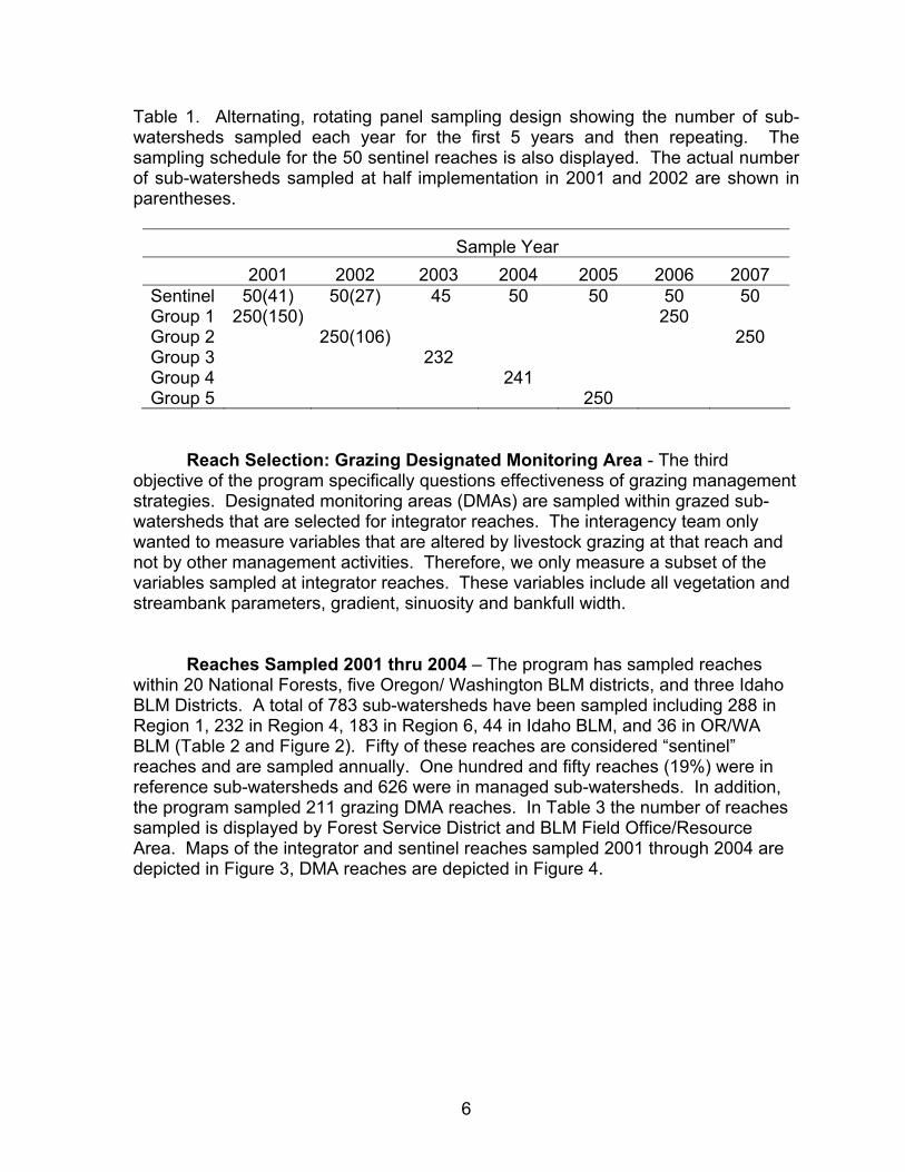
Table 1. Alternating, rotating panel sampling design showing the number of sub-watersheds sampled each year for the first 5 years and then repeating. The sampling schedule for the 50 sentinel reaches is also displayed. The actual number of sub-watersheds sampled at half implementation in 2001 and 2002 are shown in parentheses.

Sample Year 2001 2002 2003 2004 2005 2006 2007 Sentinel 50(41) 50(27) 45 50 50 50 50 Group 1 250(150) 250 Group 2 250(106) 250 Group 3 232 Group 4 241 Group 5 250

Reach Selection: Grazing Designated Monitoring Area - The third objective of the program specifically questions effectiveness of grazing management strategies. Designated monitoring areas (DMAs) are sampled within grazed sub-watersheds that are selected for integrator reaches. The interagency team only wanted to measure variables that are altered by livestock grazing at that reach and not by other management activities. Therefore, we only measure a subset of the variables sampled at integrator reaches. These variables include all vegetation and streambank parameters, gradient, sinuosity and bankfull width.

Reaches Sampled 2001 thru 2004 – The program has sampled reaches

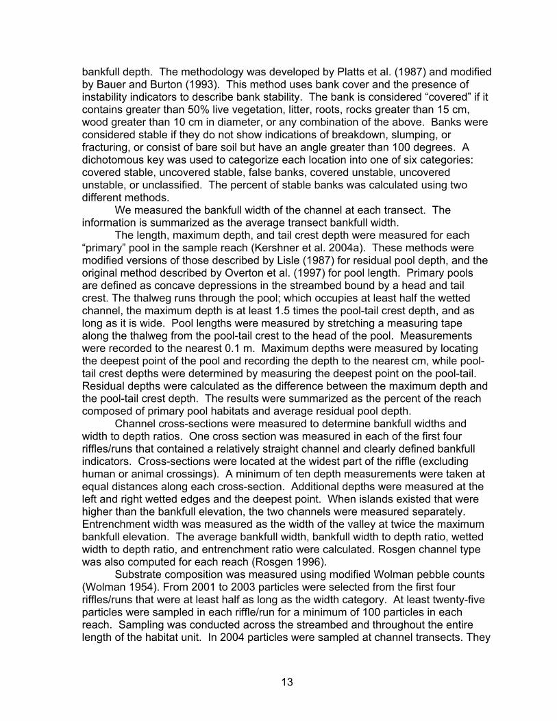
within 20 National Forests, five Oregon/ Washington BLM districts, and three Idaho BLM Districts. A total of 783 sub-watersheds have been sampled including 288 in Region 1, 232 in Region 4, 183 in Region 6, 44 in Idaho BLM, and 36 in OR/WA BLM (Table 2 and Figure 2). Fifty of these reaches are considered “sentinel” reaches and are sampled annually. One hundred and fifty reaches (19%) were in reference sub-watersheds and 626 were in managed sub-watersheds. In addition, the program sampled 211 grazing DMA reaches. In Table 3 the number of reaches sampled is displayed by Forest Service District and BLM Field Office/Resource Area. Maps of the integrator and sentinel reaches sampled 2001 through 2004 are depicted in Figure 3, DMA reaches are depicted in Figure 4.

6

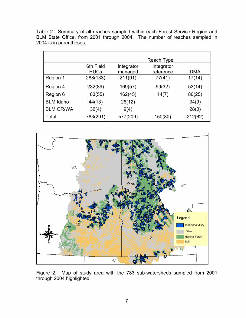
Table 2. Summary of all reaches sampled within each Forest Service Region and BLM State Office, from 2001 through 2004. The number of reaches sampled in 2004 is in parentheses.

Reach Type

6th Field HUCs

Integrator managed

Integrator reference DMA

Region 1 288(133) 211(91) 77(41) 17(14)

Region 4 232(89) 169(57) 59(32) 53(14) Region 6 183(55) 162(45) 14(7) 80(25) BLM Idaho 44(13) 26(12) 34(9) BLM OR/WA 36(4) 9(4) 28(0) Total 783(291) 577(209) 150(80) 212(62)

Figure 2. Map of study area with the 783 sub-watersheds sampled from 2001 through 2004 highlighted.

7

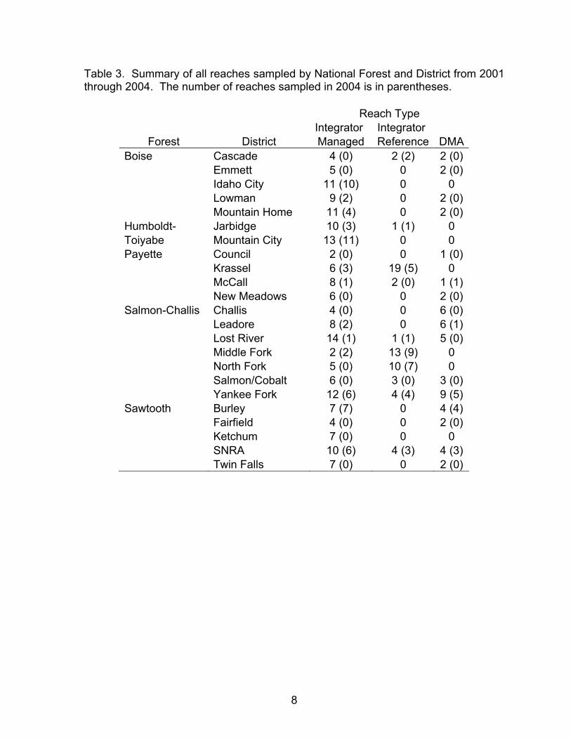
Table 3. Summary of all reaches sampled by National Forest and District from 2001 through 2004. The number of reaches sampled in 2004 is in parentheses.

Reach Type Integrator Integrator

Forest District Managed Reference DMABoise Cascade 4 (0) 2 (2) 2 (0) Emmett 5 (0) 0 2 (0) Idaho City 11 (10) 0 0 Lowman 9 (2) 0 2 (0) Mountain Home 11 (4) 0 2 (0)Humboldt- Jarbidge 10 (3) 1 (1) 0 Toiyabe Mountain City 13 (11) 0 0 Payette Council 2 (0) 0 1 (0) Krassel 6 (3) 19 (5) 0 McCall 8 (1) 2 (0) 1 (1) New Meadows 6 (0) 0 2 (0)Salmon-Challis Challis 4 (0) 0 6 (0) Leadore 8 (2) 0 6 (1) Lost River 14 (1) 1 (1) 5 (0) Middle Fork 2 (2) 13 (9) 0 North Fork 5 (0) 10 (7) 0 Salmon/Cobalt 6 (0) 3 (0) 3 (0) Yankee Fork 12 (6) 4 (4) 9 (5)Sawtooth Burley 7 (7) 0 4 (4) Fairfield 4 (0) 0 2 (0) Ketchum 7 (0) 0 0 SNRA 10 (6) 4 (3) 4 (3) Twin Falls 7 (0) 0 2 (0)

8

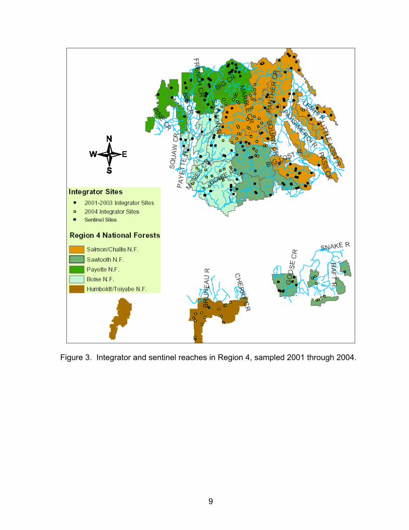
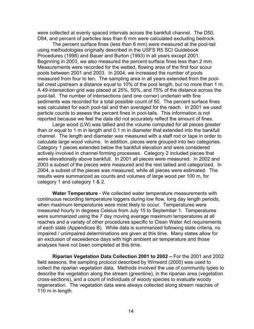
Figure 3. Integrator and sentinel reaches in Region 4, sampled 2001 through 2004.

9

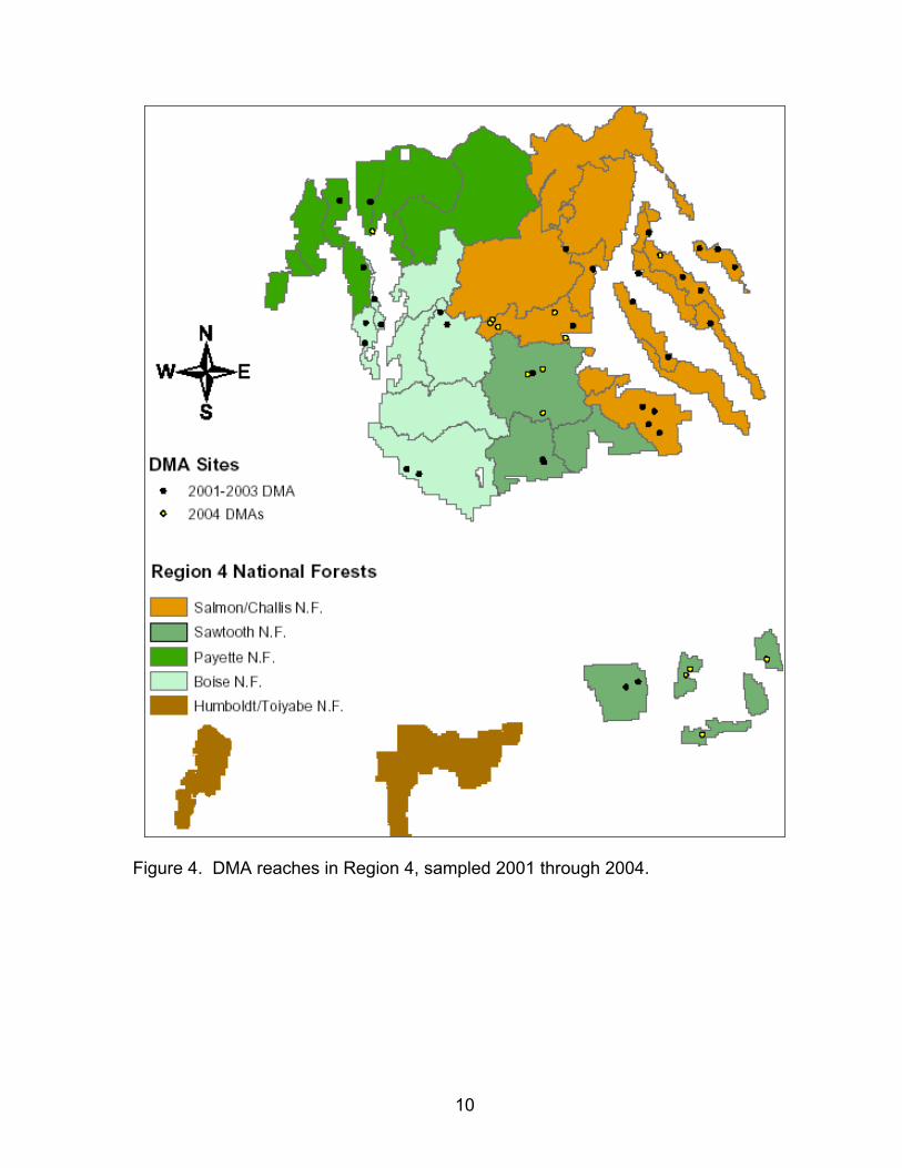
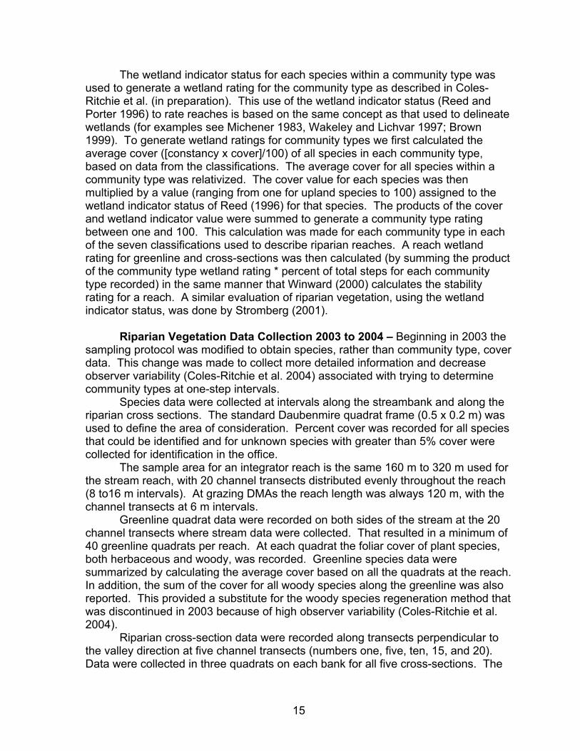
Figure 4. DMA reaches in Region 4, sampled 2001 through 2004.

10

Reach Descriptions - We used several methods to describe the location of each reach to ensure future relocation. This information is presented in the “Reach Description(s) and Photo Page” section at the end of this document (Appendix C). Written directions to the reach were recorded. A reach map was drawn that included both the stream and riparian area. Maps described the shape of the stream channel, major in-channel features, vegetation, location of tributaries, roads and other recognizable features (Harrelson et al. 1994). The Universal Transverse Mercator (UTM) coordinates at the bottom of each reach were acquired using a handheld Global Positioning System (GPS) recorder (accuracy of +/- 30 m).

Photographs were taken facing upstream and downstream from the top and bottom of each reach. Additional photographs were taken of channel and vegetation cross-sections and representative views of pools, riffles, marker location, and any unique characteristics occurring within the reach. The location and orientation of photographs were recorded so that they can be repeated during subsequent sampling. One example is included in this report and the rest of the 2003 and 2004 reach photo pages are included on the CD.

Beginning in 2003, a reach marker tag was installed at each reach. Marker tags were not placed at reaches within wilderness areas; rather a distinct natural feature was used as the reach marker. The distance and compass bearing from the natural feature to the beginning of the reach were recorded and a photo of the marker, in perspective to the reach start, was taken.

After a reach is established, a map program is used to create a topographic map of the reach location. Any other pertinent details are included on the map, such as private land boundaries, road numbers, trails, etc. This map along with the other reach description details is kept, in a folder that will be given to the crew that will resample the reach 5 years after the initial sampling. These topographic maps are also included on the accompanying CD.

Watershed Characteristics - In past years a variety of variables were computed using existing GIS coverages, to help describe the size, stream density and existing management of each watershed sampled. However, because of inconsistent and changing data layers the PIBO program has decided to finish the first 5 year rotation in 2006, and then compute all watershed characteristics at one time using consistent layers. In 2004, only percent Federal ownership, watershed area, average precipitation, and geology will be presented. In addition, we computed road densities from the most current layers to ensure reference determinations were correct. Data Collection

A combination of 23 commonly measured in-channel, 11 riparian vegetation,

and nine macroinvertebrate variables are reported for each integrator reach (Karr and Chu 1997, Kauffman et al. 1983, Platts et al. 1983, Myers and Swanson 1991, 1992, Winward 2000). Appendix A describes each summary variable and how they were computed. For more information, the sampling protocols are available on the included CD and at our website http://www.fs.fed.us/biology/fishecology/emp.

11

Since 1998, when the Effectiveness Monitoring program began, many of the methods have been modified from their original description. Many of the modifications were done to decrease observer variability by removing subjectivity and potential observer bias. We recognize that additional modifications to our present methods may become necessary with further research into stream and riparian monitoring.

Standardizing Sampling Methods – As part of our continued evolution we

have worked with the Northwest Forest Plan – Aquatic and Riparian Effectiveness Monitoring Program (AREMP) to standardize sampling methods between our programs. In 2004, both programs began using the same sampling methods for a core set of physical habitat attributes. These attributes include reach length, gradient, sinuosity, pool habitat delineation and depth, bankfull width, surface particle counts, pool-tail fines, large wood, and macroinvertebrates. These methods are also consistent with the Forest Services National Aquatic Ecological Unit Inventory guidelines. In spring of 2005 both programs are working towards common data summary variables, calculations, and metadata files, and will discuss any modifications that are needed in the methods. The overall result is that consistent information will be collected at approximately 425 reaches annually on FS and BLM lands throughout the Pacific Northwest and Columbia River Basin.

Stream Channel Measurements - Stream gradient and sinuosity were

measured to characterize the stream channel at each reach. The channel gradient at the water surface was recorded for each reach. Elevations were measured to the nearest centimeter using a surveyor’s level with tripod and a stadia rod. When the entire reach could not be surveyed from one location, we divided the reach into sections.

Bank characteristics were measured at a series of transects within the stream reach. The location of the first transect was derived by choosing a random number (k) between zero and seven. The first transect was then established (k) meters upstream of the start of the reach. Subsequent transects were located at intervals of one bankfull width category working upstream for a total of 20 to 27 transects (see protocols). All bank characteristic variables were measured on both the right and left banks.

Bank angle was measured using the procedures described by Platts et al. (1987). A clinometer and rod were used to measure the angle formed by the downward sloping stream bank as it met the stream bottom. The angle of undercut banks extended from the deepest point of the undercut to the outer edge. All angles were measured to the nearest degree with undercut banks having values less than 90 degrees and non-undercut banks greater than 90 degrees. The depth of undercut banks was measured to the nearest centimeter and extended horizontally from the deepest point of the undercut to the outer edge. The average bank angle, percent undercut banks, and average undercut depth were calculated.

Bank stability measurements were collected at each transect by observing an area of the bank 15 cm to either side of the transect location and vertically from the scour line to either the crest of the first flat above bankfull, or to twice maximum

12

bankfull depth. The methodology was developed by Platts et al. (1987) and modified by Bauer and Burton (1993). This method uses bank cover and the presence of instability indicators to describe bank stability. The bank is considered “covered” if it contains greater than 50% live vegetation, litter, roots, rocks greater than 15 cm, wood greater than 10 cm in diameter, or any combination of the above. Banks were considered stable if they do not show indications of breakdown, slumping, or fracturing, or consist of bare soil but have an angle greater than 100 degrees. A dichotomous key was used to categorize each location into one of six categories: covered stable, uncovered stable, false banks, covered unstable, uncovered unstable, or unclassified. The percent of stable banks was calculated using two different methods.

We measured the bankfull width of the channel at each transect. The information is summarized as the average transect bankfull width.

The length, maximum depth, and tail crest depth were measured for each “primary” pool in the sample reach (Kershner et al. 2004a). These methods were modified versions of those described by Lisle (1987) for residual pool depth, and the original method described by Overton et al. (1997) for pool length. Primary pools are defined as concave depressions in the streambed bound by a head and tail crest. The thalweg runs through the pool; which occupies at least half the wetted channel, the maximum depth is at least 1.5 times the pool-tail crest depth, and as long as it is wide. Pool lengths were measured by stretching a measuring tape along the thalweg from the pool-tail crest to the head of the pool. Measurements were recorded to the nearest 0.1 m. Maximum depths were measured by locating the deepest point of the pool and recording the depth to the nearest cm, while pool-tail crest depths were determined by measuring the deepest point on the pool-tail. Residual depths were calculated as the difference between the maximum depth and the pool-tail crest depth. The results were summarized as the percent of the reach composed of primary pool habitats and average residual pool depth.

Channel cross-sections were measured to determine bankfull widths and width to depth ratios. One cross section was measured in each of the first four riffles/runs that contained a relatively straight channel and clearly defined bankfull indicators. Cross-sections were located at the widest part of the riffle (excluding human or animal crossings). A minimum of ten depth measurements were taken at equal distances along each cross-section. Additional depths were measured at the left and right wetted edges and the deepest point. When islands existed that were higher than the bankfull elevation, the two channels were measured separately. Entrenchment width was measured as the width of the valley at twice the maximum bankfull elevation. The average bankfull width, bankfull width to depth ratio, wetted width to depth ratio, and entrenchment ratio were calculated. Rosgen channel type was also computed for each reach (Rosgen 1996).

Substrate composition was measured using modified Wolman pebble counts (Wolman 1954). From 2001 to 2003 particles were selected from the first four riffles/runs that were at least half as long as the width category. At least twenty-five particles were sampled in each riffle/run for a minimum of 100 particles in each reach. Sampling was conducted across the streambed and throughout the entire length of the habitat unit. In 2004 particles were sampled at channel transects. They

13

were collected at evenly spaced intervals across the bankfull channel. The D50, D84, and percent of particles less than 6 mm were calculated excluding bedrock.

The percent surface fines (less than 6 mm) were measured at the pool-tail using methodologies originally described in the USFS R5 SCI Guidebook Procedures (1998) and Bauer and Burton (1993) in all years except 2001. Beginning in 2003, we also measured the percent surface fines less than 2 mm. Measurements were recorded for the wetted, flowing area of the first four scour pools between 2001 and 2003. In 2004, we increased the number of pools measured from four to ten. The sampling area in all years extended from the pool-tail crest upstream a distance equal to 10% of the pool length, but no more than 1 m. A 49-intersection grid was placed at 25%, 50%, and 75% of the distance across the pool-tail. The number of intersections (and one corner) underlain with fine sediments was recorded for a total possible count of 50. The percent surface fines was calculated for each pool-tail and then averaged for the reach. In 2001 we used particle counts to assess the percent fines in pool-tails. This information is not reported because we feel the data did not accurately reflect the amount of fines.

Large wood (LW) was tallied and the volume computed for all pieces greater than or equal to 1 m in length and 0.1 m in diameter that extended into the bankfull channel. The length and diameter was measured with a staff rod or tape in order to calculate large wood volume. In addition, pieces were grouped into two categories. Category 1 pieces extended below the bankfull elevation and were considered actively involved in channel forming processes. Category 2 included pieces that were elevationally above bankfull. In 2001 all pieces were measured. In 2002 and 2003 a subset of the pieces were measured and the rest tallied and categorized. In 2004, a subset of the pieces was measured, while all pieces were estimated. The results were summarized as counts and volumes of large wood per 100 m, for category 1 and category 1 & 2.

Water Temperature - We collected water temperature measurements with

continuous recording temperature loggers during low flow, long day length periods, when maximum temperatures were most likely to occur. Temperatures were measured hourly in degrees Celsius from July 15 to September 1. Temperatures were summarized using the 7 day moving average maximum temperatures at all reaches and a variety of other procedures specific to Clean Water Act requirements of each state (Appendices B). While data is summarized following state criteria, no impaired / unimpaired determinations are given at this time. Many states allow for an exclusion of exceedence days with high ambient air temperature and those analyses have not been completed at this time.

Riparian Vegetation Data Collection 2001 to 2002 – For the 2001 and 2002

field seasons, the sampling protocol described by Winward (2000) was used to collect the riparian vegetation data. Methods involved the use of community types to describe the vegetation along the stream (greenline), in the riparian area (vegetation cross-sections), and a count of individuals of woody species to evaluate woody regeneration. The vegetation data were always collected along stream reaches of 110 m in length.

14

The wetland indicator status for each species within a community type was used to generate a wetland rating for the community type as described in Coles-Ritchie et al. (in preparation). This use of the wetland indicator status (Reed and Porter 1996) to rate reaches is based on the same concept as that used to delineate wetlands (for examples see Michener 1983, Wakeley and Lichvar 1997; Brown 1999). To generate wetland ratings for community types we first calculated the average cover ([constancy x cover]/100) of all species in each community type, based on data from the classifications. The average cover for all species within a community type was relativized. The cover value for each species was then multiplied by a value (ranging from one for upland species to 100) assigned to the wetland indicator status of Reed (1996) for that species. The products of the cover and wetland indicator value were summed to generate a community type rating between one and 100. This calculation was made for each community type in each of the seven classifications used to describe riparian reaches. A reach wetland rating for greenline and cross-sections was then calculated (by summing the product of the community type wetland rating * percent of total steps for each community type recorded) in the same manner that Winward (2000) calculates the stability rating for a reach. A similar evaluation of riparian vegetation, using the wetland indicator status, was done by Stromberg (2001).

Riparian Vegetation Data Collection 2003 to 2004 – Beginning in 2003 the

sampling protocol was modified to obtain species, rather than community type, cover data. This change was made to collect more detailed information and decrease observer variability (Coles-Ritchie et al. 2004) associated with trying to determine community types at one-step intervals.

Species data were collected at intervals along the streambank and along the riparian cross sections. The standard Daubenmire quadrat frame (0.5 x 0.2 m) was used to define the area of consideration. Percent cover was recorded for all species that could be identified and for unknown species with greater than 5% cover were collected for identification in the office.

The sample area for an integrator reach is the same 160 m to 320 m used for the stream reach, with 20 channel transects distributed evenly throughout the reach (8 to16 m intervals). At grazing DMAs the reach length was always 120 m, with the channel transects at 6 m intervals.

Greenline quadrat data were recorded on both sides of the stream at the 20 channel transects where stream data were collected. That resulted in a minimum of 40 greenline quadrats per reach. At each quadrat the foliar cover of plant species, both herbaceous and woody, was recorded. Greenline species data were summarized by calculating the average cover based on all the quadrats at the reach. In addition, the sum of the cover for all woody species along the greenline was also reported. This provided a substitute for the woody species regeneration method that was discontinued in 2003 because of high observer variability (Coles-Ritchie et al. 2004).

Riparian cross-section data were recorded along transects perpendicular to the valley direction at five channel transects (numbers one, five, ten, 15, and 20). Data were collected in three quadrats on each bank for all five cross-sections. The

15

quadrats were located at 3 m intervals, i.e. meters 3, 6, and 9. The cross-section species cover data were summarized for each transect on each bank, i.e. the groups of three quadrats, and those data were summarized for the entire reach.

The average cover values were used to calculate reach wetland ratings (greenline and cross-section), greenline woody cover, and weed cover (greenline and cross-section). These calculations are comparable to those used to rate community types for 2001 and 2002 data.

Trees were also counted in 3 m belts along the five riparian cross-sections noted above, and four additional cross-sections. The species and diameter-at-breast-height (DBH) were recorded for each tree greater than 4 cm DBH and taller than 1.4 m. The tree data were summarized as trees per acre and basal area per acre, for live trees and for standing dead trees.

Effective ground cover was estimated by recording the amount of bare ground at each of the 30 cross section quadrats. Bare ground was estimated by observing the cover at the four corners of the quadrat frame. The number of points (zero to four) where the pin did not contact vegetation, litter, or rock (greater than 2.5 cm) was recorded. As with the cross-section cover data, averages were first calculated for the groups of three quadrats along each cross-section, and then the ten cross-section were averaged. The percent of the reach with effective ground cover (i.e. not bare) was calculated.

A few minor things have changed in the way that we are summarizing our data. (1) For the riparian cross-section data, the “not vegetation” categories (when a quadrat lands on rock, log, trail, or road) have been dropped from the wetland rating calculations, whereas in 2003 they were included with upland designations. (2) If a specimen collected from a random quadrat was determined to be a different species than the one recorded by the technician, then that correction was made for all occurrences of that species at that reach. In 2003 the random specimens were only used to change the species for the quadrat where the specimen was collected. These changes were applied consistently to 2003 and 2004 data presented in this report.

In addition, a few species have had changes or updates in the wetland indicator status from the USDA PLANTS database (http://plants.usda.gov), so wetland ratings for a few of the 2003 reaches have changed somewhat.

Weeds and Rare Plant Species 2003 to 2004 – For each reach, the percent

cover was reported for each weed species that is listed as a noxious weed in the USDA Invaders database (http://invader.dbs.umt.edu/Noxious_Weeds/) for the state where it was observed. In addition, the percent cover for species listed as sensitive, threatened, or endangered in the National Forest or BLM area where it was observed was calculated. This information on TES species is reported directly to the National Forests where they were observed.

Macroinvertebrates - Macroinvertebrates were sampled using the protocol

recommended by the Center for Monitoring and Assessment of Freshwater Ecosystems, Utah State University (Hawkins et al. 2003). Two kick net samples were collected at randomly chosen locations within each fast-water habitat. The

16

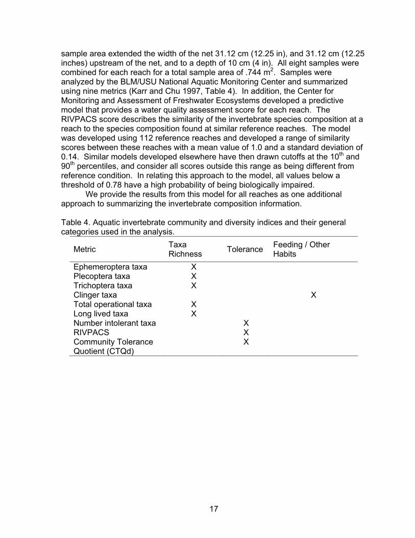
sample area extended the width of the net 31.12 cm (12.25 in), and 31.12 cm (12.25 inches) upstream of the net, and to a depth of 10 cm (4 in). All eight samples were combined for each reach for a total sample area of .744 m2. Samples were analyzed by the BLM/USU National Aquatic Monitoring Center and summarized using nine metrics (Karr and Chu 1997, Table 4). In addition, the Center for Monitoring and Assessment of Freshwater Ecosystems developed a predictive model that provides a water quality assessment score for each reach. The RIVPACS score describes the similarity of the invertebrate species composition at a reach to the species composition found at similar reference reaches. The model was developed using 112 reference reaches and developed a range of similarity scores between these reaches with a mean value of 1.0 and a standard deviation of 0.14. Similar models developed elsewhere have then drawn cutoffs at the 10th and 90th percentiles, and consider all scores outside this range as being different from reference condition. In relating this approach to the model, all values below a threshold of 0.78 have a high probability of being biologically impaired.

We provide the results from this model for all reaches as one additional approach to summarizing the invertebrate composition information.

Table 4. Aquatic invertebrate community and diversity indices and their general categories used in the analysis.

Metric Taxa Richness Tolerance Feeding / Other

Habits Ephemeroptera taxa X Plecoptera taxa X Trichoptera taxa X Clinger taxa X Total operational taxa X Long lived taxa X Number intolerant taxa X RIVPACS X Community Tolerance Quotient (CTQd)

X

17

Quality Assurance Program

Field Sampling Methods - Most large scale monitoring programs have stressed the need for a quality assurance program to insure that the information collected is technically sound, legally defensible, and useful for long-term monitoring (Mulder et al. 1999, Lazorchak et al. 1998). Our annual sampling program has included evaluations of sampling methods since 2000.

During 2000 and 2001, we conducted three separate studies to describe the precision of individual measurement techniques, variability between crews (repeatability), and temporal (seasonal) variation throughout the summer sampling season. The measurement study isolated the different components of each method to determine where errors or variability occurred. The repeatability study was conducted by having all six crews sample the same exact reaches on six streams. Summary statistics were compared between crews at each reach for all variables. An overall 95 percent confidence interval and samples sizes needed to detect changes were calculated for each variable. For the seasonal study we sampled the same reach on eight streams in June, August, and September to determine whether the measured value for each variable had changed throughout the summer sampling season. The results for stream channel (Archer et al. 2004) and riparian vegetation (Coles-Ritchie et al. 2004) attributes were published as Forest Service General Technical Reports and are included on the accompanying CD and on our website http://www.fs.fed.us/biology/fishecology/emp.

In 2002 our quality assurance sampling was conducted as part of graduate research project (Whitacre 2004). This study compared six protocols used by the USDA Forest Service and the Environmental Protection Agency to determine whether differences in protocol affect reported values for 11 physical stream attributes. Each protocol had three crews sample each of six stream reaches. This allowed for a comparison of mean estimates and observer variability among the protocols. A copy of the thesis is included on the accompanying CD and on our website.

In 2003 and 2004 we used a sampling design where approximately 25 of the 50 Sentinel reaches were sampled by two separate crews. This approach allows us to assess observer variability across the broad range of ecological conditions encountered within our study area. In 2004 revisits occurred at two different time scales to allow us to examine both observer and temporal variability. Half were revisited by a second crew within 7 days, and the other half were revisited within 30 to 40 days. This information will be summarized in future publications.

SUMMARIZED DATA

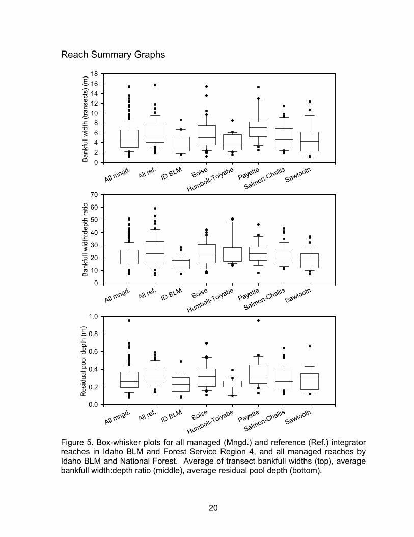
This year’s annual report provides data summaries without rigorous statistical analysis. In general, they describe the current status or baseline condition for each attribute measured. This report graphically displays the results for most variables using box and whisker plots (Figures 5 through 13). Plots were constructed for both managed and reference sub-watersheds using data from all reaches within a region and then separately for each Forest, BLM State Office, and BLM District. Three sets

18

of plots were developed for integrator reaches covering Region 1, Region 6 and OR/WA BLM, and Region 4 and ID BLM. Two sets of Grazing DMA plots were developed for Region 6 and OR/WA BLM, and Region 4 and ID BLM, but not for Region 1 due to low sample sizes. Box-Plots show the distribution of the data by depicting the median, first and third quartile (25th and 75th percentile) and the 10th and 90th percentile of the data.

We stress that samples sizes in some field units are low, so the plots should be interpreted with caution. Data summary tables are provided in Appendix B, which display all summary variables for each reach. The reaches are grouped by Forest Service District and BLM Field Office/Resource Area.

PACFISH / INFISH Comparisons - Reach data were summarized for

comparisons with seven PACFISH / INFISH Riparian Management Objectives (RMOs; PACFISH 1994). Pools per mile and wetted width to depth ratios were calculated for all reaches, except for those that were sampled dry. Bank stability and lower bank angle (percent undercut banks) were compared for meadow reaches. We defined “meadow” as having less than five pieces of large wood per 100 m of stream length and “wooded” reaches as having five or more pieces of large wood per 100 m. We defined large wood for this criterion as having a minimum size of 3 m in length and 0.1 m in width, which includes smaller pieces than the RMOs large wood criteria. Therefore, while a reach may be classified as “wooded”, no wood under the RMO classification may occur. The number of large wood pieces per mile as defined in the PACFISH and INFISH documents was compared for wooded reaches. Water temperature data were summarized for reaches using the 7 day moving average maximum temperature (AMT). We report the number of days for which the AMT was higher than 15.5° C and 17.8° C.

New Website – One of our primary goals is to provide the information that we

collect to the field units as quickly as possible. In past years this has been in the form of annual reports delivered during our spring meetings with the field units (February to April). In response to comments from many of you, we have developed a website where all summary information, original data, and associated metadata can be viewed and downloaded. Photo pages and reach description pages will also be available within the next year. We hope this will provide a quick (new year’s information will be posted by May) and convenient approach to access this information. We will be refining the website throughout 2005, so please send us suggestions on how to modify or improve it. The site can be accessed from our website at http://www.fs.fed.us/biology/fishecology/emp.

19

Reach Summary Graphs

All mngd.All re

f.ID BLM

Boise

Humbolt-ToiyabePayette

Salmon-ChallisSawtooth

Bank

full

wid

th (t

rans

ects

) (m

)

02468

1012141618

All mngd.All re

f.ID BLM

Boise

Humbolt-ToiyabePayette

Salmon-ChallisSawtooth

Bank

full

wid

th:d

epth

ratio

0

10

20

30

40

50

60

70

All mngd.All re

f.ID BLM

Boise

Humbolt-ToiyabePayette

Salmon-ChallisSawtooth

Res

idua

l poo

l dep

th (m

)

0.0

0.2

0.4

0.6

0.8

1.0

Figure 5. Box-whisker plots for all managed (Mngd.) and reference (Ref.) integrator reaches in Idaho BLM and Forest Service Region 4, and all managed reaches by Idaho BLM and National Forest. Average of transect bankfull widths (top), average bankfull width:depth ratio (middle), average residual pool depth (bottom).

20

All mngd.All re

f.ID BLM

Boise

Humbolt-ToiyabePayette

Salmon-ChallisSawtooth

% P

ools

0

20

40

60

80

100

All mngd.All re

f.ID BLM

Boise

Humbolt-ToiyabePayette

Salmon-ChallisSawtooth

Bank

ang

le (d

egre

es)

40

60

80

100

120

140

160

All mngd.All re

f.ID BLM

Boise

Humbolt-ToiyabePayette

Salmon-ChallisSawtooth

% U

nder

cut b

anks

0

20

40

60

80

100

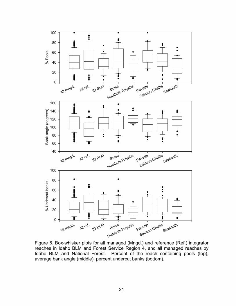
Figure 6. Box-whisker plots for all managed (Mngd.) and reference (Ref.) integrator reaches in Idaho BLM and Forest Service Region 4, and all managed reaches by Idaho BLM and National Forest. Percent of the reach containing pools (top), average bank angle (middle), percent undercut banks (bottom).

21

All mngd.All re

f.ID BLM

Boise

Humbolt-ToiyabePayette

Salmon-ChallisSawtooth

Und

ercu

t dep

th (m

)

0.0

0.1

0.2

0.3

All mngd.All re

f.ID BLM

Boise

Humbolt-ToiyabePayette

Salmon-ChallisSawtooth

% S

tabl

e ba

nks

met

hod

1

0

20

40

60

80

100

All mngd.All re

f.ID BLM

Boise

Humbolt-ToiyabePayette

Salmon-ChallisSawtooth

% S

tabl

e ba

nks

met

hod

2

0

20

40

60

80

100

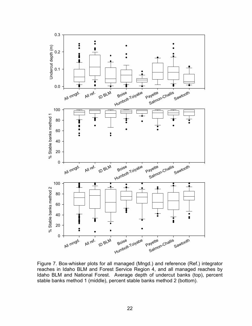
Figure 7. Box-whisker plots for all managed (Mngd.) and reference (Ref.) integrator reaches in Idaho BLM and Forest Service Region 4, and all managed reaches by Idaho BLM and National Forest. Average depth of undercut banks (top), percent stable banks method 1 (middle), percent stable banks method 2 (bottom).

22

All mngd.All re

f.ID BLM

Boise

Humbolt-ToiyabePayette

Salmon-ChallisSawtooth

% P

ool-t

ail f

ines

(<6

mm

)

0

20

40

60

80

100

All mngd.All re

f.ID BLM

Boise

Humbolt-ToiyabePayette

Salmon-ChallisSawtooth

% R

iffle

fine

s (<

6 m

m)

0

20

40

60

80

100

All mngd.All ref.

ID BLMBoise

Humbolt-ToiyabePayette

Salmon-ChallisSawtooth

Riff

le D

50 (m

m)

0

50

100

150

200

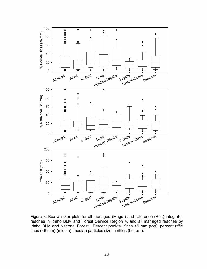
Figure 8. Box-whisker plots for all managed (Mngd.) and reference (Ref.) integrator reaches in Idaho BLM and Forest Service Region 4, and all managed reaches by Idaho BLM and National Forest. Percent pool-tail fines <6 mm (top), percent riffle fines (<6 mm) (middle), median particles size in riffles (bottom).

23

All mngd.All re

f.ID BLM

Boise

Humbolt-ToiyabePayette

Salmon-ChallisSawtooth

Riff

le D

84 (m

m)

0

100

200

300

400

All mngd.All ref.

ID BLMBoise

Humbolt-ToiyabePayette

Salmon-ChallisSawtooth

Larg

e w

ood:

cat

1 p

iece

s/10

0m

0

20

40

60

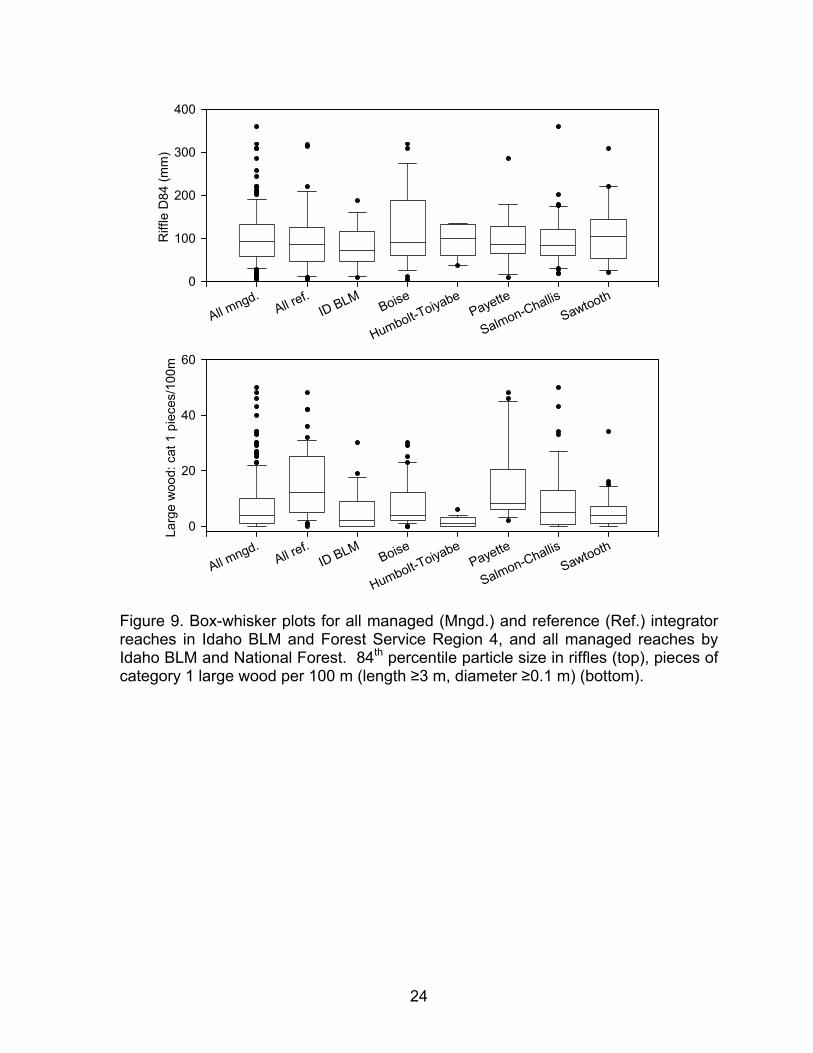
Figure 9. Box-whisker plots for all managed (Mngd.) and reference (Ref.) integrator reaches in Idaho BLM and Forest Service Region 4, and all managed reaches by Idaho BLM and National Forest. 84th percentile particle size in riffles (top), pieces of category 1 large wood per 100 m (length ≥3 m, diameter ≥0.1 m) (bottom).

24

All mngd.All ref.

ID BLMBoise

Humbolt-ToiyabePayette

Salmon-ChallisSawtooth

Gre

enlin

e w

etla

nd ra

ting

0

20

40

60

80

100

All mngd.All re

f.ID BLM

Boise

Humbolt-ToiyabePayette

Salmon-ChallisSawtooth

Rip

aria

n w

etla

nd ra

ting

0

20

40

60

80

100

All mngd.All ref.

ID BLMBoise

Humbolt-ToiyabePayette

Salmon-ChallisSawtooth

% E

ffect

ive

grou

nd c

over

0

20

40

60

80

100

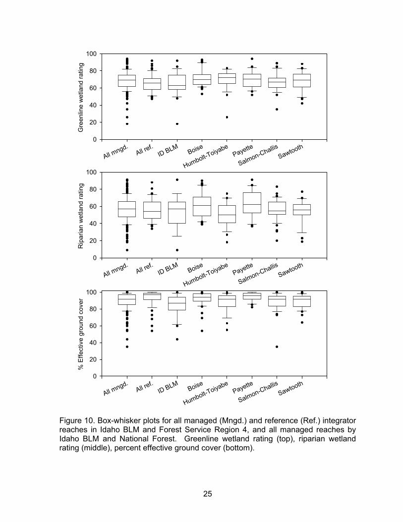
Figure 10. Box-whisker plots for all managed (Mngd.) and reference (Ref.) integrator reaches in Idaho BLM and Forest Service Region 4, and all managed reaches by Idaho BLM and National Forest. Greenline wetland rating (top), riparian wetland rating (middle), percent effective ground cover (bottom).

25

All BLMAll FS

BLM Coeur d'Alene

BLM Idaho Falls

BLM Twin Falls BoisePayette

Salmon-ChallisSawtooth

% U

nder

cut b

anks

0

20

40

60

80

100

All BLMAll FS

BLM Coeur d'Alene

BLM Idaho Falls

BLM Twin Falls BoisePayette

Salmon-ChallisSawtooth

Bank

ang

le (d

egre

es)

40

60

80

100

120

140

160

All BLMAll FS

BLM Coeur d'Alene

BLM Idaho Falls

BLM Twin Falls BoisePayette

Salmon-ChallisSawtooth

Und

ercu

t dep

th (m

)

0.0

0.1

0.2

0.3

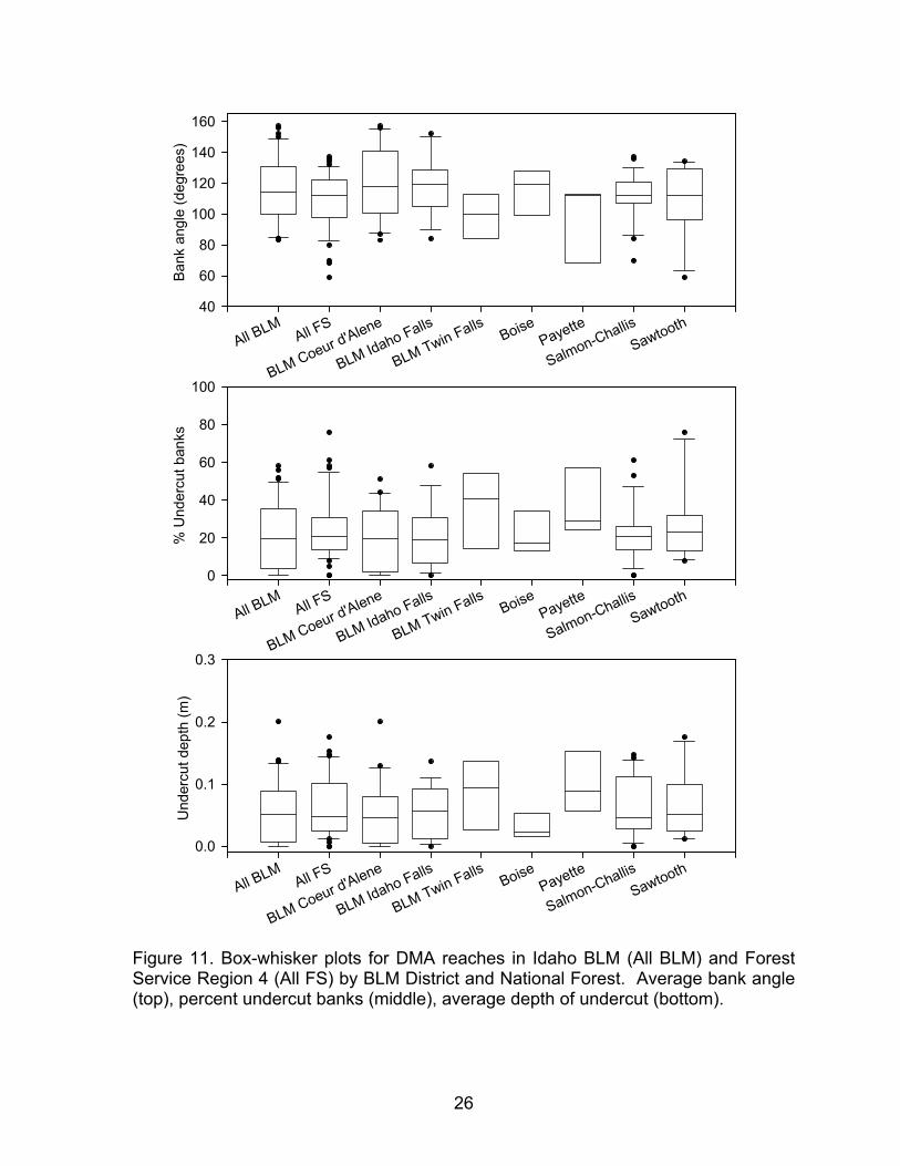
Figure 11. Box-whisker plots for DMA reaches in Idaho BLM (All BLM) and Forest Service Region 4 (All FS) by BLM District and National Forest. Average bank angle (top), percent undercut banks (middle), average depth of undercut (bottom).

26

All BLMAll FS

BLM Coeur d'Alene

BLM Idaho Falls

BLM Twin Falls BoisePayette

Salmon-ChallisSawtooth

% S

tabl

e ba

nks

met

hod

1

0

20

40

60

80

100

All BLMAll FS

BLM Coeur d'Alene

BLM Idaho Falls

BLM Twin Falls BoisePayette

Salmon-ChallisSawtooth

% S

tabl

e ba

nks

met

hod

2

0

20

40

60

80

100

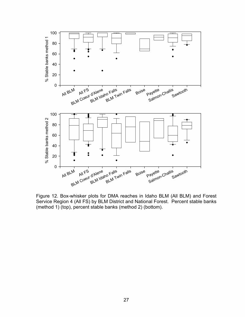
Figure 12. Box-whisker plots for DMA reaches in Idaho BLM (All BLM) and Forest Service Region 4 (All FS) by BLM District and National Forest. Percent stable banks (method 1) (top), percent stable banks (method 2) (bottom).

27

All BLMAll FS

BLM Coeur d'Alene

BLM Idaho Falls

BLM Twin Falls BoisePayette

Salmon-ChallisSawtooth

Rip

aria

n w

etla

nd ra

ting

0

20

40

60

80

100

All BLMAll FS

BLM Coeur d'Alene

BLM Idaho Falls

BLM Twin Falls BoisePayette

Salmon-ChallisSawtooth

Gre

enlin

e w

etla

nd ra

ting

0

20

40

60

80

100

All BLMAll FS

BLM Coeur d'Alene

BLM Idaho Falls

BLM Twin Falls BoisePayette

Salmon-ChallisSawtooth

% E

ffect

ive

grou

nd c

over

0

20

40

60

80

100

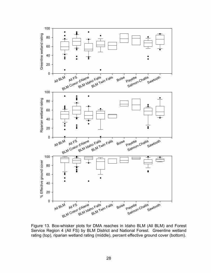
Figure 13. Box-whisker plots for DMA reaches in Idaho BLM (All BLM) and Forest Service Region 4 (All FS) by BLM District and National Forest. Greenline wetland rating (top), riparian wetland rating (middle), percent effective ground cover (bottom).

28

SPECIAL PROJECTS

Three extra projects were completed during the 2004 field season, as a continued attempt to define our data precision, and provide field units with additional beneficial data.

Region 1 Bank Disturbance Methods - In 2003, we conducted an

assessment of several methods used to measure current year streambank alteration by livestock (see publication by Heitke et al. submitted). The results were used by a FS team in Region 1 to develop a standardized sampling method for the region. In 2004 we conducted an assessment of this method along with several other approaches. This year’s assessment examined three bank alteration methods to estimate the following sources of variability: 1) among observer variability using the same method, 2) variability between methods, 3) within observer variability at a reach. For this study ten reaches where sampled on the Beaverhead-Deerlodge and Lewis and Clark NF. We expect to complete the report by April 1, 2005. Funding was provided by the USFS Fish and Aquatic Ecology Unit.

Weeds - In 2003, we began reporting the presence of weeds along the

greenline and within the riparian area. However, because only a sub-sample of the stream reach is sampled, and because weed species are often at low cover and patchy, we were interested in defining the accuracy of the weed cover data that we report. In 2004, at 34 of our sample reaches we collected additional information to help understand the accuracy of the weed information we were reporting. This information will help us determine how well our existing riparian monitoring detects the presence/absence and abundance of weed species. This study will also allow us to compute a confidence interval for the weed data presented.

Additional DMA Reaches - Idaho BLM funded us to sample 15 of their high

priority DMA’s (Designated Management Areas) each year. Reaches are selected by the field units and each reach will be re-sampled every 3 years. The information collected at these reaches will be summarized and included in the annual project annual report, but will not be included in analyses of randomly chosen PIBO reaches. This effort will help Idaho BLM meet regulatory obligations and provide useful information on the condition of these reaches.

PUBLICATIONS

The program, associated scientists, and graduate students to date have produced a number of publications to help distribute program results to land management and regulatory agency personnel, other monitoring programs, and the scientific community. Seven articles have been published and five others have been submitted. The PIBO monitoring plan (Kershner et al. 2004a) outlines the foundation and design of the program. Other articles focus on our efforts to assess observer variability in sampling methods (Archer et al. 2004; Coles-Ritchie et al. 2004; Roper et al. 2002), sources of variability associated with particle counts (Olsen et al. in

29

press), evaluations of riparian vegetation data (Coles-Ritchie dissertation; Coles-Ritchie et al. in preparation), comparisons of different sampling methods (Whitacre 2004; Heitke et al. submitted), the benefits of sampling permanent reaches (Roper et al. 2003), and a comparison of managed and reference reaches for physical habitat attributes (Kershner et al. 2004b). Finally, we have produced a “Six Year Status Report” that provides an overview of the program and summarizes accomplishments from 1998 through 2003. All publications are included on the accompanying CD and our website http://www.fs.fed.us/biology/fishecology/emp.

Archer, E. K.; Roper, B. B.; Henderson, R. C.; Bouwes, N.; Mellison, S. C.; Kershner, J. L. 2004. Testing common stream sampling methods for broad-scale, long-term monitoring. Gen. Tech. Rep. RMRS-GTR-122. Fort Collins, CO: U.S. Department of Agriculture, Forest Service, Rocky Mountain Research Station. 15 p.

Coles-Ritchie, M. C.; Henderson, R. C.; Archer, E. K.; Kennedy, C.; Kershner, J. L. 2004. Repeatability of riparian vegetation sampling methods: how useful are these techniques for broad-scale, long-term monitoring? Gen. Tech. Rep. RMRS-GTR-138. Fort Collins, CO: U.S. Department of Agriculture, Forest Service, Rocky Mountain Research Station. 18 p.

Kershner, J. L.; Archer, E. K.; Coles-Ritchie, M. C.; Cowley, E. R.; Henderson, R. C.; Kratz, K.; Quimby, C. M.; Turner, D. L.; Ulmer, D. L.; Vinson, M. R. 2004. Guide to effective monitoring of aquatic and riparian resources. Gen. Tech. Rep. RMRS-GTR-121. Ft. Collins, CO: U.S. Department of Agriculture, Forest Service, Rocky Mountain Research Station. 57 p.

Kershner, J. L.; Bouwes, N.; Roper, B. B.; Henderson, R. C. 2004. An analysis of stream habitat conditions in reference and managed watersheds on some federal lands within the Columbia Basin. North American Journal of Fisheries Management. 24: 1363–1375.

Roper, B. B.; Kershner, J. L.; Archer, E. K.; Henderson, R. C.; Bouwes, N. 2002. An evaluation of physical habitat attributes used to monitor streams. Journal of the American Water Resources Association. 38: 1637-1646.

Roper, B. B.; Kershner J. L.; Henderson R. C. 2003. The value of using permanent sites when evaluating steam attributes at the reach scale. Journal of Freshwater Ecology 18:585-592.

Whitacre, H. 2004. Comparison of USFS and EPA stream protocol methodologies and observer precision for physical habitat on Oregon and Idaho streams. Logan, UT. Utah State University: 72 p. M.S. Thesis.

30

Articles that have been submitted for publication:

Coles-Ritchie, M. C. [Submitted]. Evaluation of riparian vegetation data and associated sampling Techniques. Logan, UT. Utah State University: 204 p. Dissertation.

Coles-Ritchie, M. C.; Roberts, D. W.; Kershner, J. L.; Henderson, R. C. [Submitted]. A wetland rating system for evaluating riparian vegetation. Journal of the American Water Resources Association.

Heitke, J. D.; Henderson, R. C.; Roper, B. B.; Archer, E. K. [In Submitted]. Comparison of three streambank alteration assessment methods. Journal of Rangeland Ecology and Management.

Henderson, R. C. [Submitted]. PIBO effectiveness monitoring program: 6 year status report 1998 – 2003. Department of Agriculture, Forest Service, Rocky Mountain Research Station.

Olsen, D. S.; Roper, B. B.; Kershner, J. L.; Henderson, R. C. Archer, E. K.. [In press]. Sources of variability in pebble counts: why differences among observers may not matter. Journal of the American Water Resources Association.

31

REFERENCES

Archer, E. K.; Roper, B. B.; Henderson, R. C.; Kershner, J. L.; Mellison, S. C. 2004. Testing common stream sampling methods: how useful are these techniques for broad-scale, long-term monitoring? Gen. Tech. Rep. RMRS-GTR-122. Ft. Collins, CO: U.S. Department of Agriculture, Forest Service, Rocky Mountain Research Station. 15 p.

Bauer, S. B.; Burton, T. A. 1993. Monitoring protocols to evaluate water quality effects of grazing management on Western rangeland streams. EPA 910/R-9-93-017. Seattle, WA: U.S. Environmental Protection Agency, Water Division, Surface Water Branch, Region 10. 179 p.

Brown, S. C. 1999. Vegetation similarity and avifaunal food value of restored and natural marshes in Northern New York. Restoration Ecology. 7(1): 56-68.

Coles-Ritchie, M. C. [In preparation]. Evaluation of riparian vegetation data and associated sampling techniques. Logan: Utah State University: 204 p. Dissertation.

Coles-Ritchie, M. C.; Henderson, R. C.; Archer, E. K.; Kennedy, C.; Kershner, J. L. 2004. Repeatability of riparian vegetation sampling methods: how useful are these techniques for broad-scale, long-term monitoring? Gen. Tech. Rep. RMRS-GTR-138. Ft. Collins, CO: U.S. Department of Agriculture, Forest Service, Rocky Mountain Research Station. 18 p.

Coles-Ritchie, M. C.; Roberts, D. W.; Kershner, J. L.; Henderson, R. C. [In preparation]. A wetland rating system for evaluating riparian vegetation. Journal of the American Water Resources Association.

Harrelson, C. C.; Rawlins, C. L.; Potyondy, J. P. 1994. Stream channel reference sites: an illustrated guide to field techniques. Gen. Tech. Rep. RM-245. Fort Collins, CO: U.S. Department of Agriculture, Forest Service, Rocky Mountain Forest and Range Experimental Station. 61 p.

Hawkins, C.P.; Ostermiller, J.; Vinson, M.; Stevenson, R.J.; Olsen, J. 2003. Stream algae, invertebrate, and environmental sampling associated with biological water quality assessments: filed protocols. Department of Aquatic, Watershed, and Earth Resources, Utah State University, Logan, UT 84322-5210.

Heitke, J. D.; Henderson, R. C.; Roper, B. B.; Archer, E. K. [In preparation]. Comparison of three streambank alteration assessment methods. Journal of Rangeland Ecology and Management.

32

Karr, J. R.; Chu, E. W. 1997. Biological monitoring: essential foundation for ecological risk assessment. Human and Ecological Risk Assessment. 3(6): 993-1004.

Kauffman, J. B.; Krueger, W. C.; Vavra, M. 1983. Impacts of cattle on stream banks in northeastern Oregon. Journal of Range Management: 36(6): 683-691.

Kershner, J. L.; Archer, E. K.; Coles-Ritchie, M. C.; Cowley, E. R.; Henderson, R. C.; Kratz, K.; Quimby, C. M.; Turner, D. L.; Ulmer, D. L.; Vinson, M. R. 2004. Guide to effective monitoring of aquatic and riparian resources. Gen. Tech. Rep. RMRS-GTR-121. Ft. Collins, CO: U.S. Department of Agriculture, Forest Service, Rocky Mountain Research Station. 57 p.

Kershner, J. L.; Bouwes, N.; Roper, B. B.; Henderson, R. C. 2004. An analysis of stream habitat conditions in reference and managed watersheds on some federal lands within the Columbia basin. North American Journal of Fisheries Management. 24(4): 1363–1375.

Lazorchak, J. M.; Klemm, D. J.; Peck, D. V. 1998. Environmental monitoring and assessment program – surface waters: field operations and methods for measuring ecological condition of wadeable streams. EPA/620/R-94/004F. Washington, DC: U.S. Environmental Protection Agency.

Lisle, T. E. 1987. Using “residual depths” to monitor pool depths independently of discharge. Res. Note PSW-394. Berkeley, CA: U.S. Department of Agriculture, Forest Service, Pacific Southwest Forest and Range Experiment Station. 4 p.

Meyers, T. J.; Swanson, J. 1991. Aquatic habitat condition index, stream type, and livestock bank damage in Northern Nevada. Water Resources Bulletin. 27(4): 667-677.

Meyers, T. J.; Swanson, J. 1992. Variation of stream stability with stream type and livestock bank damage in Northern Nevada. Water Resources Bulletin. 28(4): 743-754.

Michener, M. C. 1983. Wetland site index for summarizing botanical studies. Wetlands. 3: 180-191.

Montgomery, D. R.; MacDonald, L. H. 2002. Diagnostic approach to stream channel assessment and monitoring. Journal of the American Water Resources Association. 38: 1-16.

33

Mulder, B. S.; Noon, B. R.; Spies, T. A.; Raphael, M. G.; Palmer, C. J.; Olsen, A. R.; Reeves, G. H.; Welsh, H. H. 1999. The strategy and design of the Effectiveness Monitoring Program for the Northwest Forest Plan. Gen. Tech. Rep. PNW-GTR-437. Portland, OR: U.S. Department of Agriculture, Forest Service, Pacific Northwest Station. 61p.

Olsen, D. S.; Roper, B. B.; Kershner, J. L.; Henderson, R. C. Archer, E. K.. [In press]. Sources of variability in pebble counts: why differences among observers may not matter. Journal of the American Water Resources Association.

Overton, C. K.; Wollrab, S. P.; Roberts, B. C.; Radko, M. A.; 1997. R1/R4 (Northern and intermountain regions) fish and fish habitat standard inventory procedures handbook. Gen. Tech. Rep. INT-GTR-346. Ogden, UT: U.S. Department of Agriculture, Forest Service, Intermountain Research Station. 142 p.

PACFISH (Pacific Anadromous Fisheries Habitat), U.S. Forest Service and U.S. Bureau of Land Management. 1994. Environmental assessment for the implementation of interim strategies for managing anadromous fish-producing watersheds in Eastern Oregon, Washington, Idaho, and portions of California. Washington, D.C: U.S. Department of Agriculture, Forest Service. 68 p.

Platts, W. S.; Nelson, R. L.; Casey, O.; Crispin, V. 1983. Riparian stream habitat conditions on Tabor Creek, Nevada, under grazed and ungrazed conditions. Proceedings of the Annual Conference Western Association of Fish and Wildlife Agencies 63: 162-174.

Platts, W.S.; Armour, C.; Booth, G. D.; Bryant, M.; Bufford, J. L.; Cuplin, P.; Jensen, S.; Lienkaemper, G. W.; Minshall, G. W.; Monsen, S. P.; Nelson, R. L.; Sedell, J. R.; Tuhy, J. S. 1987. Methods for evaluating riparian habitats with applications to management. Gen. Tech. Rep. INT-221. Ogden, UT: U.S. Department of Agriculture, Forest Service, Intermountain Research Station. 177 p.

Quigley, T. M.; Arbelbide, S. J. (tech. Eds) 1997. An assessment of ecosystem components in the interior Columbia basin and portions of the Klamath and Great Basins. Gen. Tech. Rep. PNW-GTR-405. Portland, OR: U.S. Department of Agriculture, Forest Service, Pacific Northwest Research Station. 4 vol.

Reed, J.; Porter B. 1996. Draft revision of 1988 national list of plant species that occur in wetlands: national summary. Washington, DC: U.S. Department of the Interior, Fish and Wildlife Service. 215 p.

34

Roper, B. B.; Kershner, J. L.; Archer, E. K.; Henderson, R. C.; Bouwes, N. 2002. An evaluation of physical habitat attributes used to monitor streams. Journal of the American Water Resources Association. 38: 1637-1646.

Roper, B. B.; Kershner, J. L.; Henderson, R. C. 2003. The value of using permanent sites when evaluating steam attributes at the reach scale. Journal of Freshwater Ecology 18(4): 585-592.

Rosgen, D. L. 1996. Applied River Morphology. Wildland Hydrology, Pagosa Springs, CO.

Stevens, D. L. 1997. Variable density grid-based sampling designs for continuous spatial populations. Environmetrics 8:167-195.

Stromberg, J. C. 2001. Biotic integrity of Platanus wrightii riparian forests in Arizona: first approximation. Forest Ecology and Management. 142: 251-266.

U.S. Department of Agriculture, Forest Service. 1976. National Forest Management Act (NFMA).

U.S. Department of Agriculture, Forest Service, Region 5. 1998. R5 SCI Stream Condition Inventory Guidebook. Version 4.0.

Wakeley, J. S.; Lichvar, R. W.; 1997. Disagreements between plot-based prevalence indices and dominance ratios in evaluations of wetland vegetation. Wetlands 17(2): 301-309.

Whitacre, H. 2004. Comparison of USFS and EPA stream protocol methodologies and observer precision for physical habitat on Oregon and Idaho streams. Logan, UT. Utah State University: 72 p. M.S. Thesis.

Wingett, R. N.; Magnum, F. A. 1979. Biotic condition index: integrated biological, physical, and chemical parameters for management. Ogden, UT: U.S. Department of Agriculture, Forest Service, Intermountain Region.

Winward, A. H. 2000. Monitoring the vegetation resources in riparian areas. Gen. Tech. Rep. RMRS-GTR-47. Ogden, UT: U.S. Department of Agriculture, Forest Service, Rocky Mountain Research Station. 49 p.

Wolman, M. G. 1954. A method of sampling coarse riverbed material. Transactions of the American Geophysical Union. 35(6): 951-956.

35

APPENDIX A - DEFINITIONS AND DESCRIPTIONS OF SUMMARY VARIABLES

36

REACH DEFINITIONS Designated monitoring area (DMA) reach - Reach identified by field unit personnel as the location utilized for livestock grazing implementation monitoring. Integrator reach – downstream-most low-gradient (< 3%) reach within ICBEMP 6th field HUC. Integrator reaches are randomly selected and sampled as part of the five year rotating panel sampling design. Sentinel reach – One of 50 integrator or 12 DMA reaches sampled annually. WATERSHED CHARACTERISTICS Average precipitation (mm) – Average precipitation (mm) for the sub-watershed as computed by the Interior Columbia Basin Ecosystem Management Project. Elevation (ft) – Integrator reach elevation (ft). Identified from 1:24000 topographic maps. FS:BLM ownership (%) – Percent Forest Service and BLM land ownership upstream of integrator reach. Geology – Primary geology for each sub-watershed upstream of sample reach. The dominant geology was determined by ICBEMP geologic layers, and categorized as sedimentary, metamorphic, granitic, or volcanic. Management category – Integrator reaches designated as managed or reference. Reference reaches require road densities less than 0.5 km/km2, riparian road densities less than 0.25 km/km2 , no grazing within 30 years, and no mining upstream of the integrator reach. Rosgen channel type – Channel type computed from Figure 5-3 Classification Key for Natural Rivers in Applied River Morphology by Dave Rosgen. Watershed area (ha) – Total area (ha) of watershed upstream of integrator reach. STREAM CHANNEL VARIABLES Average bank angle (degrees) – Average of all bank angle measurements (degrees).

37

Average bankfull width (m) (cross-sections) – Average of the bankfull widths (m) from the channel cross-sections. Average transect bankfull width (m) – Average of the bankfull widths (m) measured at each of the 20+ transects. Average bankfull width:depth ratio – The average ratio of bankfull width / average bankfull depth, for all channel cross-sections. The average bankfull depth was calculated as the (bankfull width / total bankfull area). Average residual pool depth (m) – Average of the residual pool depths for all pools. Average undercut depth (m) - Sum of all undercut depths (m) / total number of transects. Average wetted width:depth ratio (AWR) - The average ratio of wetted width / average water depth, for all channel cross-sections. The average water depth was calculated as the (wetted width / total wetted area). Bedrock – Particles >4096mm. Entrenchment ratio – The average of four cross-section entrenchment ratios. The ratio for each cross-section was calculated as valley width at twice maximum bankfull depth / bankfull width. Gradient (%) – Elevation change of the water surface from the bottom of the reach to the top of the reach divided by the reach length (measured along the thalweg), expressed a percent. Large wood: category 1 pieces / 100 m (>3m * 0.1m) – Number of pieces per 100 meters of stream length. This was calculated as the total number of pieces (>3m in length and 0.1m in diameter) divided by the reach length, *100. Some portion of the piece must be within the bankfull channel and below the bankfull elevation. Large wood: category 1 pieces / 100 m (>1m * 0.1m) – Number of pieces per 100 meters of stream length. This was calculated as the total number of pieces (>1m in length and 0.1m in width) divided by the reach length, * 100. Some portion of the piece must be within the bankfull channel and below the bankfull elevation. Large wood: category 1 volume / 100 m (>1m * 0.1m) – Volume of category 1 pieces in m3 per 100 meters of stream length.

38

Large wood: category 1 & 2 pieces / 100 m (>1m * 0.1m) – Number of pieces per 100 meters of stream length. This was calculated as the total number of pieces (>1m in length and 0.1m in width) divided by the reach length, * 100. Includes all category 1 pieces plus pieces that are within the bankfull channel but above the bankfull elevation (category 2). Large wood: category 1 & 2 volume / 100 m (>1m * 0.1m) – Volume of category 1 & 2 pieces in m3 per 100 meters of stream length. Pools (%) - Sum of all pool lengths / reach length. Pools/mile - Total number of pools / reach length * 1609. Pool-tail fines <2 mm and <6 mm (%) - Percent surface fines for each pool were calculated as the average of (((fines grid 1 / total number of intersections) + (fines grid 2 / total number of intersections) + (fines grid 3 / total number of intersections)) * 100). All four pools were averaged for the reach. Fines were considered, 6 mm for all years except 2001 when this measurement was not conducted. Percent surface fines, 2 mm were also calculated 2003-2004. Riffle D50 (2001-2003) - The D50 (millimeters) is derived from modified Wolman Pebble Counts. Fifty percent of the substrate particles sampled are less than this size. Values reported without bedrock (particles >4096mm). Riffle D84 (2001-2003) - The D84 (millimeters) is derived from modified Wolman Pebble Counts. Eighty four percent of the substrate particles sampled are less than this size. Values reported without bedrock (particles >4096mm). Riffle fines <6 mm (%) – The percentage of particles from modified Wolman Pebble Counts that were < 6 mm. Values reported without bedrock (particles >4096 mm). Sinuosity – Reach length measured along the thalweg divided by the straight valley length from the bottom of the reach to the top of the reach. Stable banks method 1 (%) – Each bank stability measurement is rated covered stable, covered unstable, uncovered stable, uncovered unstable, or false bank. The percent stable banks is calculated as (number of covered stable, uncovered stable, and false bank measurements / total number of measurements). Stable banks method 2 (%) – Method 2 uses the same data as method 1. The percent stable banks is calculated as the (number of covered stable and false bank measurements / total number of measurements). The category uncovered stable is considered unstable using this method.

39

Transect D50 (2004) - The D50 (millimeters) is derived from modified Wolman Pebble Counts. Fifty percent of the substrate particles sampled are less than this size. Values reported without bedrock (particles >4096mm). Transect D84 (2004) - The D84 (millimeters) is derived from modified Wolman Pebble Counts. Eighty four percent of the substrate particles sampled are less than this size. Values reported without bedrock (particles >4096mm). Transect fines <6 mm (%) – The percentage of particles from modified Wolman Pebble Counts that were <6 mm. Values reported without bedrock (particles >4096mm). Undercut banks (%) - Number of locations with bank angles < 90 degrees and an undercut depth of > 5 cm / total number of bank measurements. Wood/mile - Number of pieces per mile of stream length. This was calculated as the total number of pieces (>11m in length and 0.28m in diameter) divided by the reach length, *1609. Some portion of the piece must be within the bankfull channel. RIPARIAN VEGETATION Cross-section weed cover (%) – The percent cover, from the greenline to a distance of 9.5 m, of each species that is listed as a noxious weed as per Rice (2004) for the state where it was observed. Previous to 2003, community type cover data were collected, so information on weeds was not available. Cross-section wetland rating – A measure of the abundance of obligate wetland species in the riparian area, with 100 indicating all obligate wetland species and 0 being all upland species. The rating is calculated for the reach by summing the product of the average cover of each species and a value corresponding to the species’ wetland indicator status. Data through 2002 were based on a variable riparian width, which included only what was considered riparian, up to a maximum of 27.5 m on each side of the stream. Beginning in 2003 the sample area was a fixed width of 9.5 m on each side of the greenline (including the greenline).

40

Effective ground cover (%) – The percent of the riparian area (not including the greenline) with effective ground cover, which was defined as live vegetation cover (within 1 m of ground), rock (> 2.5 cm), or litter. Data were collected along the riparian cross-sections and averaged for the reach. Data through 2002 were based on a variable riparian width, which included only what was considered riparian, up to a maximum of 27.5 m, on each side of the stream. Beginning in 2003 the sample area was a fixed width of 9.5 m on each side of the greenline (excluding the greenline because some bare ground is expected, such as on sand bars). Greenline weed cover (%) – The percent cover along the greenline, of each species that is listed as a noxious weed, as with the “cross-section weed cover (%)” described above. Greenline wetland rating – A measure of the abundance of obligate wetland species along the streambank, with 100 indicating all obligate wetland species and 0 being all upland species. The rating is calculated for the reach by summing the product of the average cover of each species and a value corresponding to the species’ wetland indicator status. Greenline woody cover – The percent cover of woody species along the greenline. These could be any woody species, such as willows or pines. Previous to 2003, community type cover data were collected, which did not provide accurate information about woody cover. Large trees (>50 cm DBH) per acre – The number of trees per acre with a diameter of greater than 50 cm. This number is an extrapolation of the number of large trees observed at the sample reach within 9.5 m of the greenline (including the greenline). Tree data were collected beginning in 2004. Live tree basal area per acre – The sum of the basal areas (3.14 *[dbh/2]2) for all live trees (>4 cm DBH) observed within 9.5 m of the greenline (including the greenline), extrapolated to a 1 acre area. Tree data were collected beginning in 2004. Small trees (<50 cm DBH) per acre – The number of trees per acre with a diameter between 4 and 50 cm. This number is an extrapolation of the number of small trees observed at the sample reach within 9.5 m of the greenline (including the greenline). Tree data were collected beginning in 2004. Standing dead basal area per acre – The sum of the basal areas (3.14 *[dbh/2]2) for all dead trees (>4 cm DBH) observed within 9.5 m of the greenline (including the greenline), extrapolated to a 1 acre area. Tree data were collected beginning in 2004.

41

Standing dead per acre – The number of standing dead trees (>4 cm DBH) per acre. This number is an extrapolation of the number of dead trees observed at the sample reach within 9.5 m of the greenline (including the greenline). Tree data were collected beginning in 2004. MACROINVERTEBRATES Community Tolerance Quotient (CTQd) – This index was developed by Winget and Mangum (1979) and has been widely used by the USFS and BLM throughout the western United States. Taxa are assigned a tolerant quotient from 2 to 108. Taxa assigned low tolerance quotients are found only in high quality unpolluted water and taxa assigned large tolerant quotients are found in severely polluted waters. The CTQd is a dominance weighted community tolerance quotient (CTQd). Number of clinger taxa – Number of “clinger” taxa. These taxa typically cling to the tops of rocks and may be impacted by sedimentation or abundant algal growths. Number of Ephemeroptera taxa – Number of Mayfly taxa. Number of intolerant taxa – Number of “intolerant” taxa. The number of intolerant taxa normally declines with decreasing water quality. Number of long-lived taxa – Number of “long-lived” taxa. Long-lived taxa typically have 2-3 year life cycles and respond negatively to human disturbance. Number of Plecoptera taxa – Number of Stonefly taxa. Number of Tricoptera taxa – Number of Caddisfly taxa. RIVPACS – Observed taxa at a site / expected taxa for that strata. RIVPACS employs a predictive model that compares the number of macroinvertebrate fauna to be expected in high quality habitat to the number found at a given site. Scores > 0.78 indicate good quality habitat whereas scores < 0.78 indicate poorer quality habitat. Total OTU (Operational Taxonomic Unit) richness – Total number of taxa collected within a reach. Taxa richness normally decreases with decreasing water quality, although organic enrichment can cause an increase in the number of pollution tolerant taxa.

42

WATER TEMPERATURE Oregon (DEQ) – Water temperature data for reaches in Oregon are summarized using the 7-day moving average maximum temperature (AMT). We report the number of days for which the AMT was higher than 10.0° C, 12.8° C, and 17.8° C. Washington (DOE) – Water temperature data for reaches in Washington are summarized using the daily maximum temperature (DMT). We report the number of days where the DMT was above 16° C, 18° C, 21° C, and 22° C. Idaho (DEQ) – Water temperature data for reaches in Idaho are summarized using the DMT and daily average temperature (DAT). We report the number of days for which the DMT is above 22° C and the DAT above19° C. Montana (DEQ) – Water temperature data for reaches in Montana are summarized using the 7-day AMT. We report the number of days for which the AMT exceeds 10°

C, 15° C, and 21° C. Nevada (DEP) – Water temperature data for reaches in Nevada are summarized using the DMT. We report the number of days for which the DMT is greater than or equal to 20° C. Utah (DEQ) – Water temperature data for reaches in Nevada are summarized using the DMT. We report the number of days for which the DMT exceeds 20° and 27° C. PACFISH / INFISH Riparian Management Objectives - The 7-day moving average maximum temperature was calculated for each site. We present the number of days where the 7D-MAMT exceeded 15.5 and 17.8oC. The data is presented in the PACFISH table.

43

APPENDIX B – REACH SUMMARY TABLES

In the original version of the report, this appendix included summary tables for all reaches sampled between 2001 and 2004. We removed tables from this version to save space. The information can be found in the original copies, on our website, or by contacting us at PIBO@fs.fed.us.

44

APPENDIX C – REACH DESCRIPTION(S) AND PHOTO PAGE

45

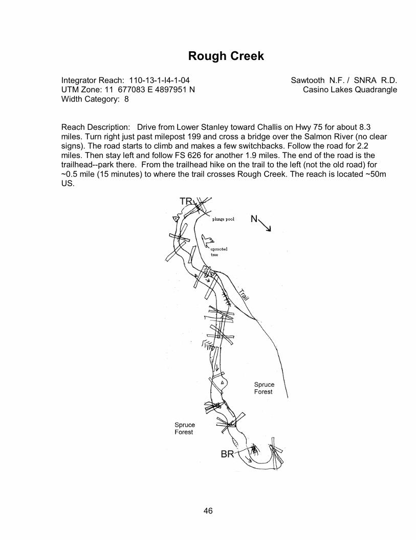
Rough Creek

Integrator Reach: 110-13-1-I4-1-04 UTM Zone: 11 677083 E 4897951 N Width Category: 8

Sawtooth N.F. / SNRA R.D.Casino Lakes Quadrangle

Reach Description: Drive from Lower Stanley toward Challis on Hwy 75 for about 8.3 miles. Turn right just past milepost 199 and cross a bridge over the Salmon River (no clear signs). The road starts to climb and makes a few switchbacks. Follow the road for 2.2 miles. Then stay left and follow FS 626 for another 1.9 miles. The end of the road is the trailhead--park there. From the trailhead hike on the trail to the left (not the old road) for ~0.5 mile (15 minutes) to where the trail crosses Rough Creek. The reach is located ~50m US.

46

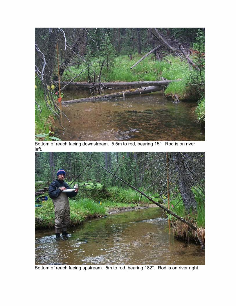
Bottom of reach facing downstream. 5.5m to rod, bearing 15°. Rod is on river left.

Bottom of reach facing upstream. 5m to rod, bearing 182°. Rod is on river right.

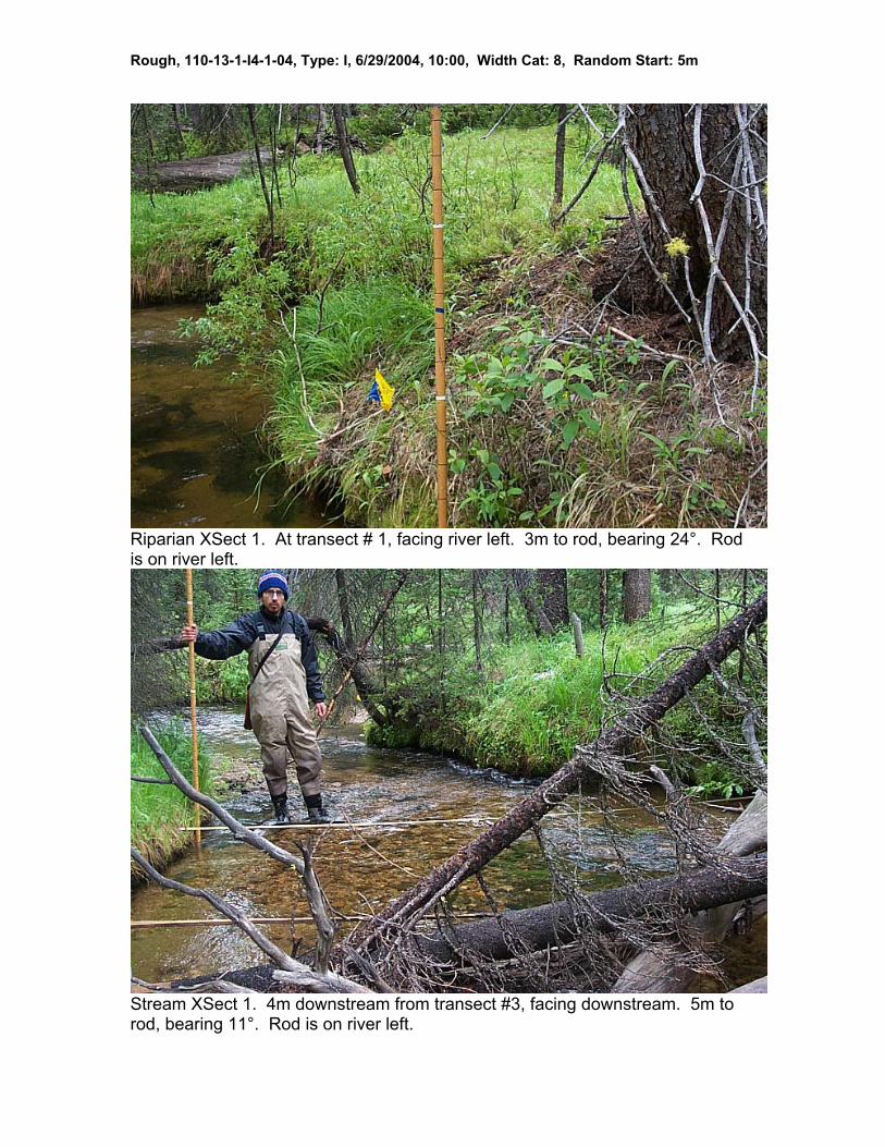
Rough, 110-13-1-I4-1-04, Type: I, 6/29/2004, 10:00, Width Cat: 8, Random Start: 5m

Riparian XSect 1. At transect # 1, facing river left. 3m to rod, bearing 24°. Rod is on river left.

Stream XSect 1. 4m downstream from transect #3, facing downstream. 5m to rod, bearing 11°. Rod is on river left.

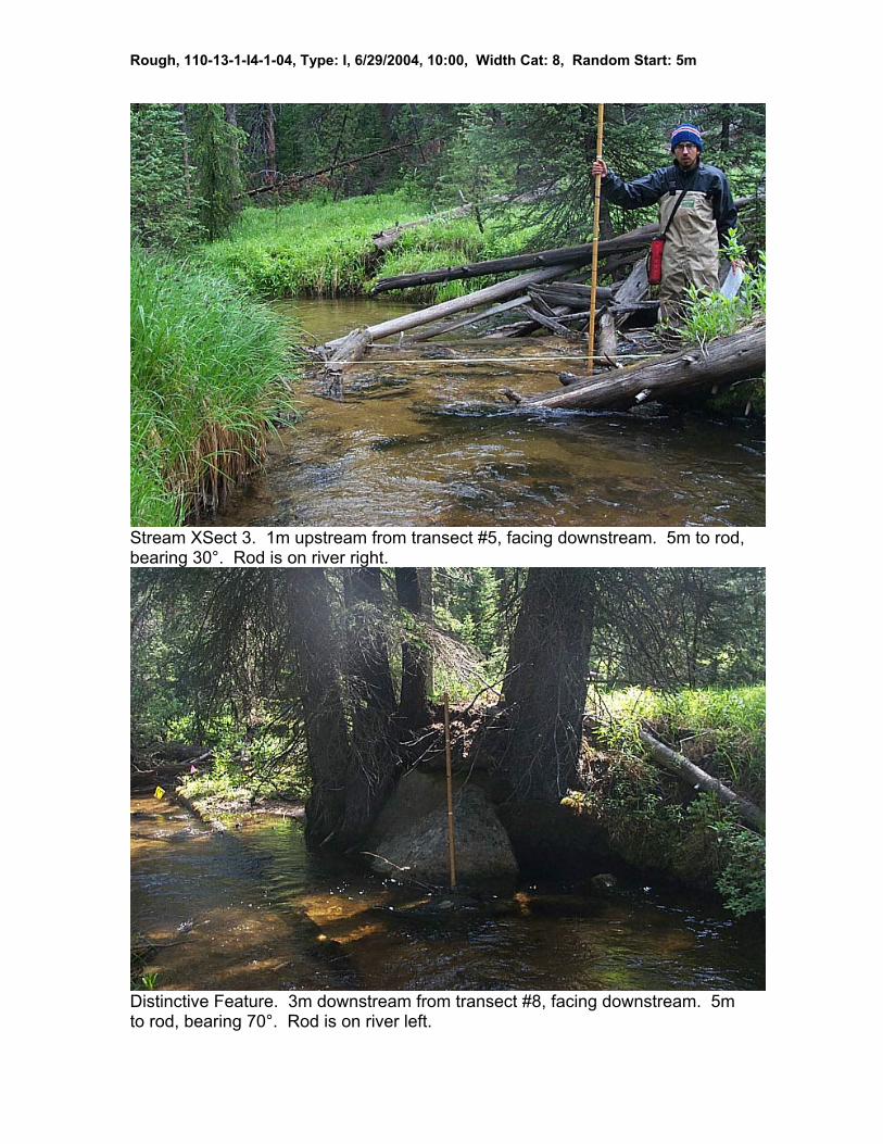
Rough, 110-13-1-I4-1-04, Type: I, 6/29/2004, 10:00, Width Cat: 8, Random Start: 5m

Stream XSect 3. 1m upstream from transect #5, facing downstream. 5m to rod, bearing 30°. Rod is on river right.

Distinctive Feature. 3m downstream from transect #8, facing downstream. 5m to rod, bearing 70°. Rod is on river left.

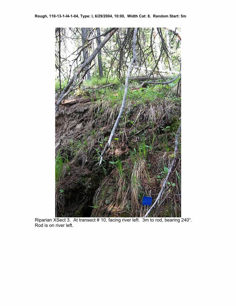
Rough, 110-13-1-I4-1-04, Type: I, 6/29/2004, 10:00, Width Cat: 8, Random Start: 5m

Riparian XSect 3. At transect # 10, facing river left. 3m to rod, bearing 240°. Rod is on river left.

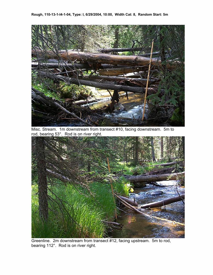
Rough, 110-13-1-I4-1-04, Type: I, 6/29/2004, 10:00, Width Cat: 8, Random Start: 5m

Misc. Stream. 1m downstream from transect #10, facing downstream. 5m to rod, bearing 53°. Rod is on river right.

Greenline. 2m downstream from transect #12, facing upstream. 5m to rod, bearing 112°. Rod is on river right.

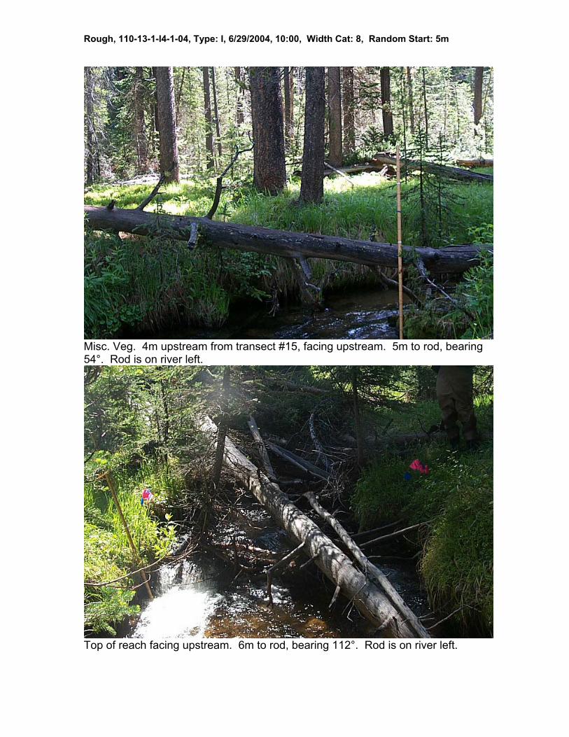
Rough, 110-13-1-I4-1-04, Type: I, 6/29/2004, 10:00, Width Cat: 8, Random Start: 5m

Misc. Veg. 4m upstream from transect #15, facing upstream. 5m to rod, bearing 54°. Rod is on river left.

Top of reach facing upstream. 6m to rod, bearing 112°. Rod is on river left.

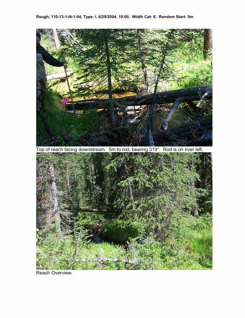
Rough, 110-13-1-I4-1-04, Type: I, 6/29/2004, 10:00, Width Cat: 8, Random Start: 5m

Top of reach facing downstream. 5m to rod, bearing 319°. Rod is on river left.

Reach Overview.

If you have any questions, please contact us:

Fish & Aquatic Ecology Unit 860 North 1200 East

Logan, UT 84321

Name Title Phone E-mail Rick Henderson Project Leader (435) 755-3578 rhenderson01@fs.fed.us Eric Archer Field Team Leader (435) 755-3565 earcher@fs.fed.us Boyd Bouwes GIS specialist (208) 634-0816 babouwes@fs.fed.us Marc Coles-Ritchie Riparian Ecologist (435) 755-3597 mcolesritchie@fs.fed.us

To view our annual report and effectiveness monitoring study plan, Please visit our website:

http://www.fs.fed.us/biology/fishecology/emp