Embed Size (px)
Citation preview
IRC TechNote
Refrigerant Inventory Determination
Industrial Refrigeration Consortium College of Engineering
University of Wisconsin-Madison
August 2004

2 © 2004
About the IRC
The IRC is a collaborative effort between the University of Wisconsin-Madison and industry. Together we share a common goal of improving safety, efficiency, and productivity of industrial refrigeration systems and technologies. We realize this goal by conducting applied research, delivering knowledge transfer, and providing technical assistance.
The IRC offers its members a unique resource built upon professional staff that have academic qualifications, technical expertise, and practical experience with industrial refrigeration systems and technologies. We constantly strive to provide our members with high-quality objective information that is not biased by an affiliation with any particular organization.
Currently, the following industry leaders are reaping the benefits of membership in the IRC: Alliant Energy, General Mills, Kraft Foods, NOR-AM Cold Storage, Sargento Foods, Schoep’s Ice Cream, Tropicana Products, Wells’ Dairy, Xcel Energy. Complementing our end-user members in the IRC are the United States Occupational Safety & Health Administration (OSHA) and the Environmental Protection Agency (EPA) are also members.
For more information on membership, browse our website at: www.irc.wisc.edu or contact us at [email protected].
The IRC is wholly funded by external funds.
3 © 2004
Refrigerant Inventory Determination
Background As an end-user, do I need to worry about determining the quantity of refrigerant in my system? The short answer to this question is yes! There reasons why industrial refrigeration end-users need to know the refrigerant inventory of their systems is varied and depends on the type of refrigerant in use. For end-users with halocarbon refrigeration systems, refrigerant inventory determination and tracking of refrigerant emissions is required for compliance with regulations enacted by Congress as part of Title VI of the Clean Air Act (CAA) Amendments of 1990. Section 608 of the CAA defines specific requirements for industrial refrigeration systems using either Class I or Class II1 ozone depleting substances to determine system refrigerant inventories and track refrigerant leakage from the system. Specifically, Section 608 requires owners or operators of an industrial process or commercial refrigeration system to repair refrigerant leaks when the loss would exceed 35 percent of the total system charge over a 12-month period. To enable leak rate estimates, the system's refrigerant inventory must be known. In situations where the refrigeration plant is a large built-up system, determining refrigerant inventory is best accomplished by summing the quantity of refrigerant residing in the components that comprise the system. Further information on these regulations can be found in the EPA's guidance document (EPA 1995). For end-users that operate industrial refrigeration systems using anhydrous ammonia as the refrigerant, estimating and documenting the normal and maximum refrigerant inventory takes on heightened importance. The heightened importance is attributable to regulations that govern the use of toxic substances (including anhydrous ammonia) in industrial processes. The two most significant regulations that arise in this case are OSHA’s Process Safety Management (PSM) standard and EPA’s Risk Management Program (RMP). In cases where the quantity of refrigerant exceeds a defined maximum limit, end-users are required to comply with the provisions of both the PSM and RMP standards. Even in cases where the total inventory of a system is less than the threshold quantity, inventory calculations are still useful for assessing process risks.
Motivation Our motivation in preparing this TechNote stems from the numerous end-user inquiries we have received in the past with questions relating to inventory determination for their refrigeration systems. It is in direct response to these inquiries that we have prepared this TechNote. Our primary goal for this TechNote is provide a complete description of the principles and methods associated with determining the refrigerant inventory in industrial refrigeration systems. Based on inventory estimates for individual components in a system, we can arrive at a system total inventory estimate by summing the component-level refrigerant inventories. We begin this TechNote by providing background on the importance of inventory determination. Because anhydrous ammonia is the dominant refrigerant used in industrial systems, we review the properties of ammonia next. Finally, principles and techniques for determining the refrigerant inventory for the major components that make up an industrial refrigeration system are presented. Example calculations are provided in the Appendix.
1 Class I refrigerants are pure component or mixtures of chlorofluorocarbons (CFCs). Class II refrigerants are pure component or mixtures of hydrochlorofluorocarbons (HFCs).

4 © 2004
Process Safety Management OSHA’s Process Safety Management (PSM) Standard (29 CFR 1910.119) is a comprehensive safety program aimed at preventing or minimizing the likelihood of large-scale catastrophic chemical incidents involving flammable and highly hazardous substances. Section (a) of the PSM standard establishes the “applicability” of processes required to comply with the provisions of the Standard. Plants using anhydrous ammonia in any process are required to develop and implement a process safety management program if the inventory of their system(s) exceeds the threshold quantity (TQ) of 10,000 lbm as listed in Appendix A of the PSM Standard. Section (b) of the PSM Standard defines a “process” as:
“any activity involving a highly hazardous chemical including any use, storage, manufacturing, handling, or the on-site movement of such chemicals, or combination of these activities. For purposes of this definition, any group of vessels which are interconnected and separate vessels which are located such that a highly hazardous chemical could be involved in a potential release shall be considered a single process.”
Clearly, an ammonia refrigeration system fits the definition of a “process” and any plant with a refrigeration system having a charge in excess of the threshold quantity (TQ for ammonia is 10,000 lbm) is required to develop and implement a PSM program. It is also noteworthy to point out that a plant having two or more refrigeration systems in close proximity with individual charges less than the TQ (10,000 lbm) but with an additive quantity in excess of the TQ would also be subject to the provisions of the PSM Standard even though their individual charge may be less than the TQ. EPA’s Risk Management Planning (RMP) program (40 CFR 68) is aimed at protecting the public and environment from damages that would arise from the accidental release of highly hazardous or flammable substances. The RMP program requires that plants with covered processes estimate the footprint outside of the plant boundary that would, potentially, be impacted by a release of a highly hazardous chemical. The TQ of ammonia required for submission of an RMP program is also 10,000 lbm. In addition, many of the requirements for RMP mirror OSHA’s PSM program. Once I determine that my plant has over 10,000 lbm of ammonia, I don’t need to go any further with inventory determination - right? No! For those plants having covered processes, section (d) of the Standard (Process Safety Information) requires maintaining up-to-date estimates of their system inventory2. In addition to the total inventory for a system, both the normal and maximum system inventory for major system components (such as vessels) are needed as inputs to off-site consequence analyses RMP compliance. The first step in determining whether or not your facility is required to develop and implement PSM and RMP programs is to establish an estimate of the refrigerant inventory for your process (system). If the refrigerant inventory for your system exceeds the threshold quantity, you are covered by both PSM and RMP.
Properties of Anhydrous Ammonia Anhydrous ammonia is the refrigerant of choice in the industrial arena. Ammonia offers several advantages such as high system efficiency, good heat transfer performance, no ozone depletion 2 Technically, section (d)(2)(C) of the PSM Standard requires maintaining estimates of the “maximum intended inventory.” For refrigeration, the process is “closed” so that the system inventory is synonymous with “maximum intended inventory.” However, the maximum intended inventory of individual components is important and useful information as input to process hazards analyses.
5 © 2004
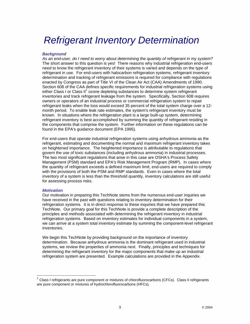
potential, and no contribution to global warming. With respect to refrigerant inventory determination, ammonia has unique properties that require us to focus our attention during the process of inventory estimation. Density is a property that represents the mass per unit volume (e.g. lbm/ft3) of a substance. By knowing the density of refrigerant at a given point in our system and the corresponding volume of that component or subsystem, we can estimate the refrigerant inventory for that component or subsystem. By adding the inventory (mass) of refrigerant that resides in individual components, an estimate of the entire system charge can be established. Figure 1 shows the variation in the density of liquid ammonia with temperature and extent of subcooling. As the temperature increases, the refrigerant density decreases. The decrease in density is a rather modest 8 lbm/ft3 over a 140ºF temperature range (about an 18% overall decrease in density or a 0.13% decrease per ºF increase in temperature).
-40 -20 0 20 40 60 80 10036
37
38
39
40
41
42
43
44
45
Saturation Temperature [°F]
Liqu
id D
ensi
ty [
lbm
/ft3 ]
Anhydrous ammonia
Saturated liquid
10°F subcooling
20°F subcooling
30°F subcooling
Figure 1: Variation in density for liquid-phase anhydrous ammonia.
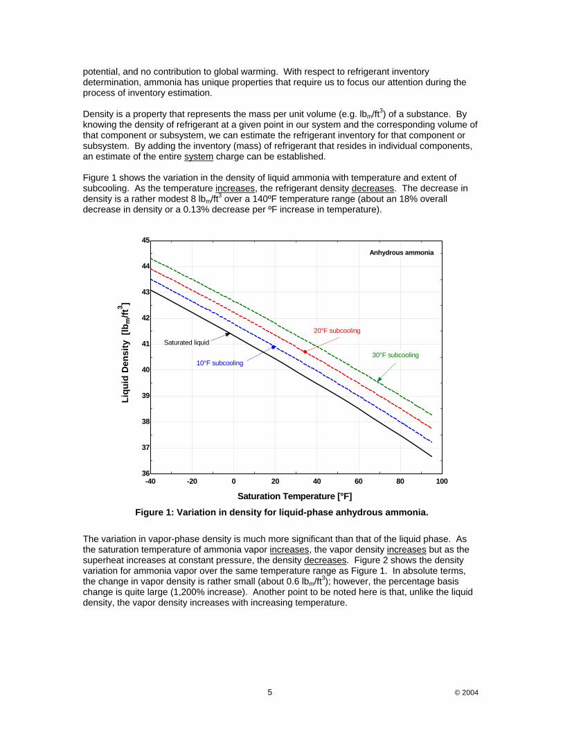
The variation in vapor-phase density is much more significant than that of the liquid phase. As the saturation temperature of ammonia vapor increases, the vapor density increases but as the superheat increases at constant pressure, the density decreases. Figure 2 shows the density variation for ammonia vapor over the same temperature range as Figure 1. In absolute terms, the change in vapor density is rather small (about 0.6 lbm/ft3); however, the percentage basis change is quite large (1,200% increase). Another point to be noted here is that, unlike the liquid density, the vapor density increases with increasing temperature.
6 © 2004
-40 -20 0 20 40 60 80 1000
0.1
0.2
0.3
0.4
0.5
0.6
0.7
Saturation Temperature [°F]
Vapo
r Den
sity
[lb
m/ft
3 ]
Anydrous Ammonia
Saturated vapor
10°F Superheat
20°F Superheat
Figure 2: Variation in density for vapor-phase anhydrous ammonia.
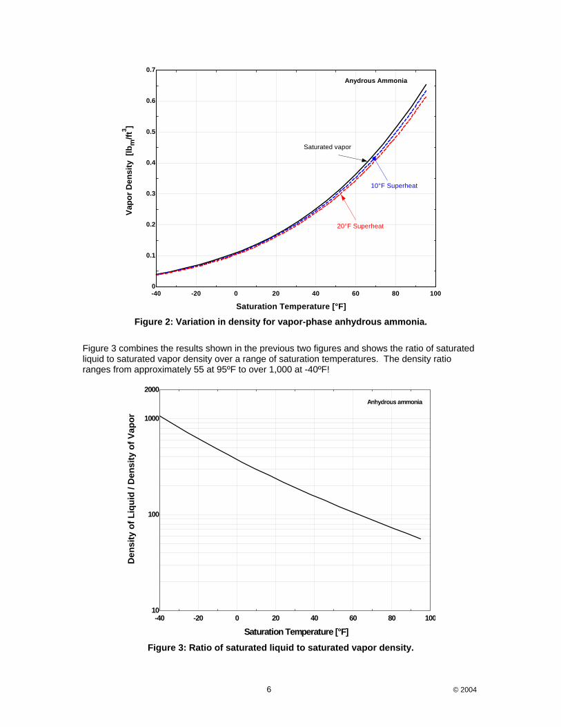
Figure 3 combines the results shown in the previous two figures and shows the ratio of saturated liquid to saturated vapor density over a range of saturation temperatures. The density ratio ranges from approximately 55 at 95ºF to over 1,000 at -40ºF!
-40 -20 0 20 40 60 80 10010
100
1000
2000
Saturation Temperature [°F]
Den
sity
of L
iqui
d / D
ensi
ty o
f Vap
or
Anhydrous ammonia
Figure 3: Ratio of saturated liquid to saturated vapor density.

7 © 2004
A corollary to density is its inverse, specific volume. The specific volume represents the volume of a substance occupied by a unit mass (ft3/lbm). Because the density of refrigerant in a vapor state can be quite small, specific volume is often used as an alterative measure to establish the relationship between the refrigerant’s volume and mass. What can we conclude from looking at the density of anhydrous ammonia in both the liquid and vapor phase? The major conclusion is that we need to focus our attention on those places in a refrigeration system that hold liquid phase refrigerant in order to obtain the best estimate of overall system charge. Why? Well the relative mass of refrigerant associated with vapor phase refrigerant will be very small. We underscore this point by comparing mass of refrigerant associated with vapor vs. liquid in the examples provided the Appendix.
Inventory Estimation Now that we know to focus our attention on those areas of a refrigeration system containing liquid refrigerant, let’s consider prioritizing those portions of the system and review methods for determining the quantity contained within those parts of the system. Figure 4 shows a simplified flow diagram illustrating the major components of a multi-temperature level two-stage compression refrigeration system. Most industrial refrigeration systems will have the single greatest mass of refrigerant contained within the system’s vessels; however, end-users with systems that have a footprint covering a large area may find that the mass in liquid piping exceeds the refrigerant inventory in vessels. Heat exchangers (condensers and evaporators) and liquid piping will also contain appreciable inventories of refrigerant mass as well. Based on the properties of ammonia, expect to find minimal refrigerant inventory in the vapor spaces of vessels and vapor piping.
Equalizerline
EvaporativeCondenser(s)
MediumTemperatureEvaporator(s)
LowTemperatureEvaporator(s) Medium
TemperatureRecirculator/Intercooler
LowTemperatureRecirculator
BoosterCompressor(s)
High-StageCompressor(s)
HighPressureReceiver
1
2
3
4
5
5’6
4’
7
5’’
4’’
T
DX Evap
8
Figure 4: Multiple temperature level two-stage compression refrigeration system.
8 © 2004
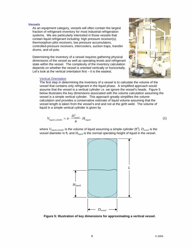
Vessels As an equipment category, vessels will often contain the largest fraction of refrigerant inventory for most industrial refrigeration systems. We are particularly interested in those vessels that contain liquid refrigerant including: high pressure receiver(s), thermosiphon pilot receivers, low pressure accumulators, controlled-pressure receivers, intercoolers, suction traps, transfer drums, and oil pots. Determining the inventory of a vessel requires gathering physical dimensions of the vessel as well as operating levels and refrigerant state within the vessel. The complexity of the inventory calculation depends on whether the vessel is oriented vertically or horizontally. Let’s look at the vertical orientation first – it is the easiest.
Vertical Orientation The first step in determining the inventory of a vessel is to calculate the volume of the vessel that contains only refrigerant in the liquid phase. A simplified approach would assume that the vessel is a vertical cylinder i.e. we ignore the vessel’s heads. Figure 5 below illustrates the key dimensions associated with the volume calculation assuming the vessel is a simple vertical cylinder. This approach greatly simplifies the volume calculation and provides a conservative estimate of liquid volume assuming that the vessel length is taken from the vessel’s end and not at the girth weld. The volume of liquid in a simple vertical cylinder is given by
2
, 4vessel
liquid cylinder liquidDV Hπ= ⋅ ⋅ (1)
where Vliquid,cylinder is the volume of liquid assuming a simple cylinder (ft3), Dvessel is the vessel diameter in ft, and Hliquid is the normal operating height of liquid in the vessel.
Figure 5: Illustration of key dimensions for approximating a vertical vessel.
L
Hliquid
Dvessel
9 © 2004
The inventory can then be approximated by the product of the liquid volume and the liquid refrigerant density for the given operating pressure/temperature in the vessel.
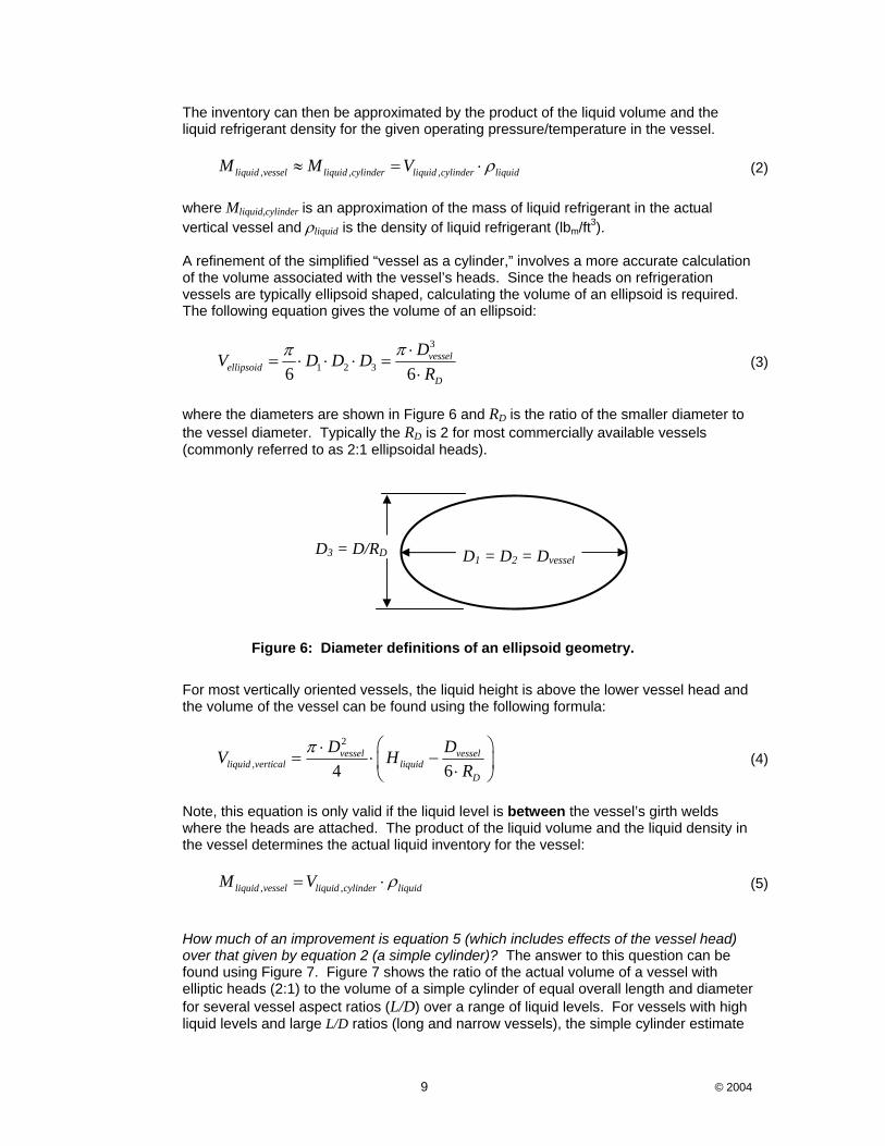
, , ,liquid vessel liquid cylinder liquid cylinder liquidM M V ρ≈ = ⋅ (2) where Mliquid,cylinder is an approximation of the mass of liquid refrigerant in the actual vertical vessel and ρliquid is the density of liquid refrigerant (lbm/ft3). A refinement of the simplified “vessel as a cylinder,” involves a more accurate calculation of the volume associated with the vessel’s heads. Since the heads on refrigeration vessels are typically ellipsoid shaped, calculating the volume of an ellipsoid is required. The following equation gives the volume of an ellipsoid:
3
1 2 36 6vessel
ellipsoidD
DV D D DR
ππ ⋅= ⋅ ⋅ ⋅ =
⋅ (3)
where the diameters are shown in Figure 6 and RD is the ratio of the smaller diameter to the vessel diameter. Typically the RD is 2 for most commercially available vessels (commonly referred to as 2:1 ellipsoidal heads).
Figure 6: Diameter definitions of an ellipsoid geometry.
For most vertically oriented vessels, the liquid height is above the lower vessel head and the volume of the vessel can be found using the following formula:
2
, 4 6vessel vessel
liquid vertical liquidD
D DV HR
π ⎛ ⎞⋅= ⋅ −⎜ ⎟⋅⎝ ⎠
(4)
Note, this equation is only valid if the liquid level is between the vessel’s girth welds where the heads are attached. The product of the liquid volume and the liquid density in the vessel determines the actual liquid inventory for the vessel:
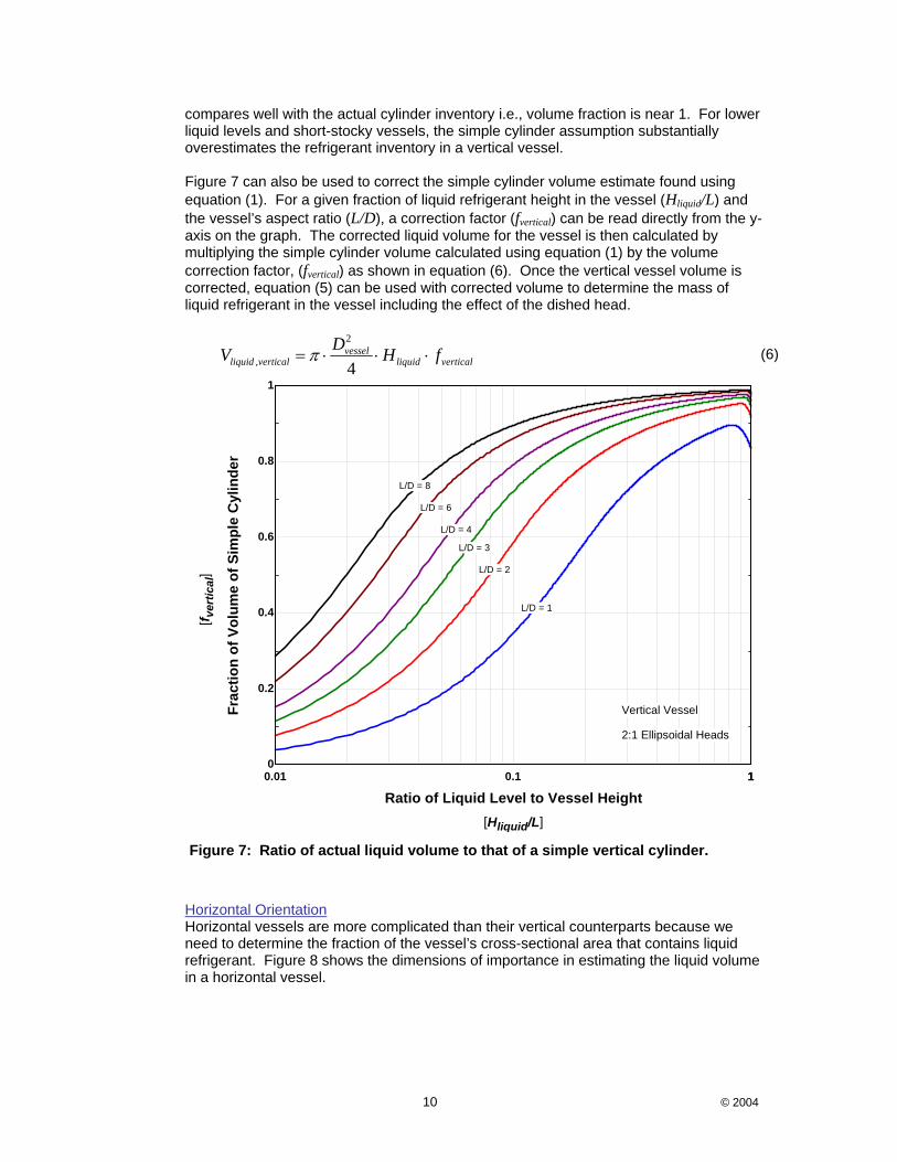
, ,liquid vessel liquid cylinder liquidM V ρ= ⋅ (5) How much of an improvement is equation 5 (which includes effects of the vessel head) over that given by equation 2 (a simple cylinder)? The answer to this question can be found using Figure 7. Figure 7 shows the ratio of the actual volume of a vessel with elliptic heads (2:1) to the volume of a simple cylinder of equal overall length and diameter for several vessel aspect ratios (L/D) over a range of liquid levels. For vessels with high liquid levels and large L/D ratios (long and narrow vessels), the simple cylinder estimate
D1 = D2 = DvesselD3 = D/RD
10 © 2004
compares well with the actual cylinder inventory i.e., volume fraction is near 1. For lower liquid levels and short-stocky vessels, the simple cylinder assumption substantially overestimates the refrigerant inventory in a vertical vessel. Figure 7 can also be used to correct the simple cylinder volume estimate found using equation (1). For a given fraction of liquid refrigerant height in the vessel (Hliquid/L) and the vessel’s aspect ratio (L/D), a correction factor (fvertical) can be read directly from the y-axis on the graph. The corrected liquid volume for the vessel is then calculated by multiplying the simple cylinder volume calculated using equation (1) by the volume correction factor, (fvertical) as shown in equation (6). Once the vertical vessel volume is corrected, equation (5) can be used with corrected volume to determine the mass of liquid refrigerant in the vessel including the effect of the dished head.
2
, 4vessel
liquid vertical liquid verticalDV H fπ= ⋅ ⋅ ⋅ (6)
0.01 0.1 110
0.2
0.4
0.6
0.8
1
Ratio of Liquid Level to Vessel Height
Frac
tion
of V
olum
e of
Sim
ple
Cyl
inde
r
L/D = 1
L/D = 2
L/D = 3
L/D = 4
L/D = 6
L/D = 8
2:1 Ellipsoidal Heads
Vertical Vessel
[f ver
tical
]
[Hliquid/L]
Figure 7: Ratio of actual liquid volume to that of a simple vertical cylinder.
Horizontal Orientation Horizontal vessels are more complicated than their vertical counterparts because we need to determine the fraction of the vessel’s cross-sectional area that contains liquid refrigerant. Figure 8 shows the dimensions of importance in estimating the liquid volume in a horizontal vessel.

11 © 2004
Figure 8: Illustration of key dimensions approximating a horizontal vessel.
Starting with a simple “vessel as a cylinder” analysis again, the equations and methodology for determining the cross-sectional area, volume, and mass of a vessel that contains liquid are given by equations (7), (8) and (10), respectively. Equation 7 relies on the curve shown in Figure 9 to correct the gross cross-sectional area of the horizontal vessel for a given liquid level as follows:
2
, 4vessel
liquid cylinder liquidDA fπ= ⋅ ⋅ (7)
where fliquid is taken from the y-axis of Figure 9 for the liquid height to diameter ratio (Hliquid/Dvessel) in the vessel.
0 0.2 0.4 0.6 0.8 10
0.2
0.4
0.6
0.8
1
Ratio of Liquid Height to Vessel Diameter
Frac
tion
of C
ylin
der C
ross
-sec
tiona
l Are
a w
ith L
iqui
d
Horizontal Vessel
Figure 9: Fraction of liquid in a horizontal vessel.
Hliquid
L
Dvessel
12 © 2004
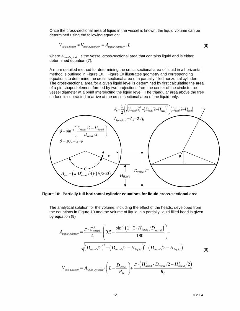
Once the cross-sectional area of liquid in the vessel is known, the liquid volume can be determined using the following equation:
, , ,liquid vessel liquid cylinder liquid cylinderV V A L≈ = ⋅ (8) where Aliquid,cylinder is the vessel cross-sectional area that contains liquid and is either determined equation (7). A more detailed method for determining the cross-sectional area of liquid in a horizontal method is outlined in Figure 10. Figure 10 illustrates geometry and corresponding equations to determine the cross-sectional area of a partially filled horizontal cylinder. The cross-sectional area for a given liquid level is determined by first calculating the area of a pie-shaped element formed by two projections from the center of the circle to the vessel diameter at a point intersecting the liquid level. The triangular area above the free surface is subtracted to arrive at the cross-sectional area of the liquid-only.
Figure 10: Partially full horizontal cylinder equations for liquid cross-sectional area. The analytical solution for the volume, including the effect of the heads, developed from the equations in Figure 10 and the volume of liquid in a partially liquid filled head is given by equation (9)
( )
( ) ( ) ( )
( )
12
,
22
2 3
, ,
sin 1 20.5
4 180
2 2 2
2 2
liquid vesselvesselliquid cylinder
vessel vessel liquid vessel liquid
liquid vessel liquidvesselliquid vessel liquid cylinder
D D
H DDA
D D H D H
H D HDV A LR R
π
π
−⎛ ⎞− ⋅⋅ ⎜ ⎟= ⋅ − −⎜ ⎟⎝ ⎠
− − ⋅ −
⋅ ⋅ −⎛ ⎞= ⋅ − +⎜ ⎟
⎝ ⎠
(9)
1 2sin
2180 2
vessel liquid
vessel
D HD
φ
θ φ
− −⎛ ⎞= ⎜ ⎟
⎝ ⎠= − ⋅
Hliquid
θ
φ
( ) ( )2 4 360pie vesselA Dπ θ= ⋅
( ) ( ) ( )22
,
1 2 2 22
2
tri vessel vessel vessel liquidliquid
liquid cylinder pie tri
A D D H D H
A A A
⎛ ⎞= ⋅ − − ⋅ −⎜ ⎟⎝ ⎠
= − ⋅
Dvessel /2

13 © 2004
Regardless of the method used for determining the volume of liquid in a horizontal vessel, the mass of liquid in the vessel is determined with the following equation:
, ,liquid vessel liquid vessel liquidM V ρ= ⋅ (10)
Similar to the vertical vessels, Figure 11 shows the ratio of volume of a partially-filled horizontal vessel (with 2:1 elliptical heads) to that of simple horizontal cylinder. For large aspect ratios (L/D=4 or higher), the simple cylinder approximation is within 10% of the actual volume for a vessel with elliptical heads. Figure 11 allows correction of the estimated liquid volume from equation (8) to account for 2:1 ellipsoidal heads. The corrected liquid volume is calculated by multiplying the simplified volume determined in equation (8) by the correction factor taken from Figure 11 (fhorizontal) for vessel’s length to diameter ratio (L/D) and the liquid height to diameter ratio (Hliquid/D).
, ,liquid vessel liquid cylinder horizontalV A L f= ⋅ ⋅ (11)
0.01 0.1 110.5
0.6
0.7
0.8
0.9
1
Ratio of Liquid Level to Vessel Diameter
Frac
tion
of V
olum
e of
Sim
ple
Cyl
inde
r
L/D = 1
L/D = 2
L/D = 3L/D = 4
L/D = 6L/D = 8
2:1 Ellipsoidal Heads
Horizontal Vessel
[f hor
izon
tal]
[Hliquid/Dvessel]
Figure 11: Ratio of actual liquid volume to that of a partially filled horizontal cylinder.
14 © 2004
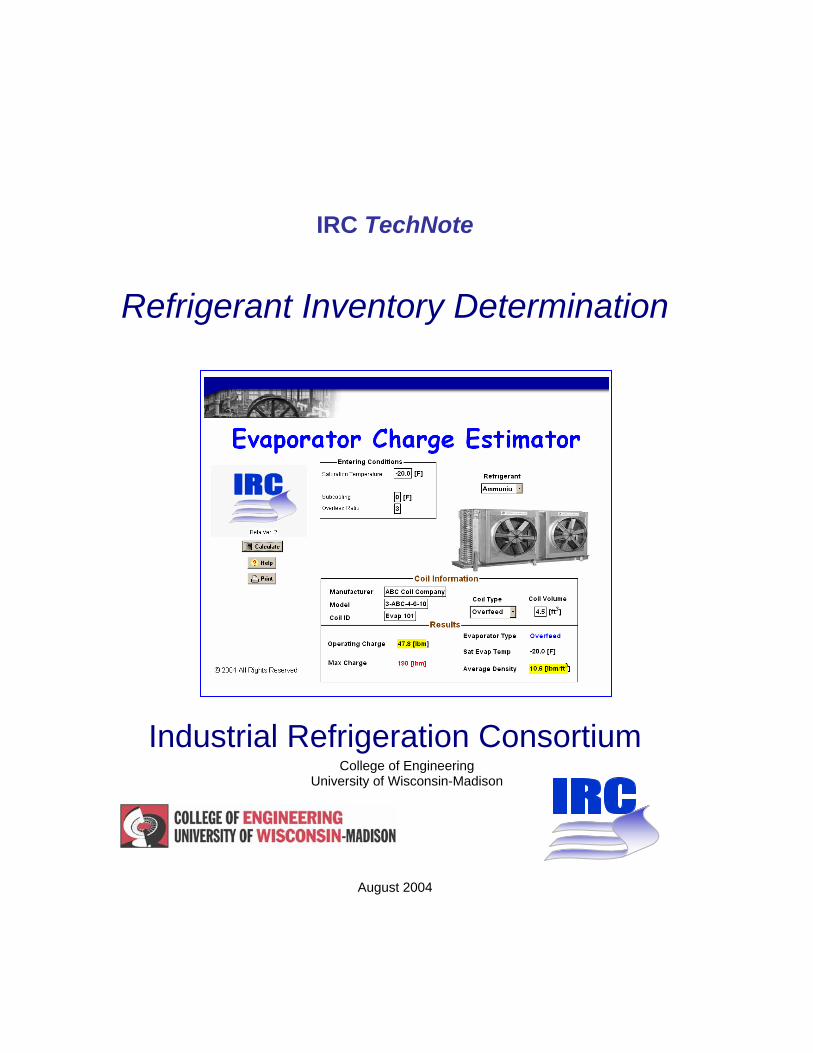
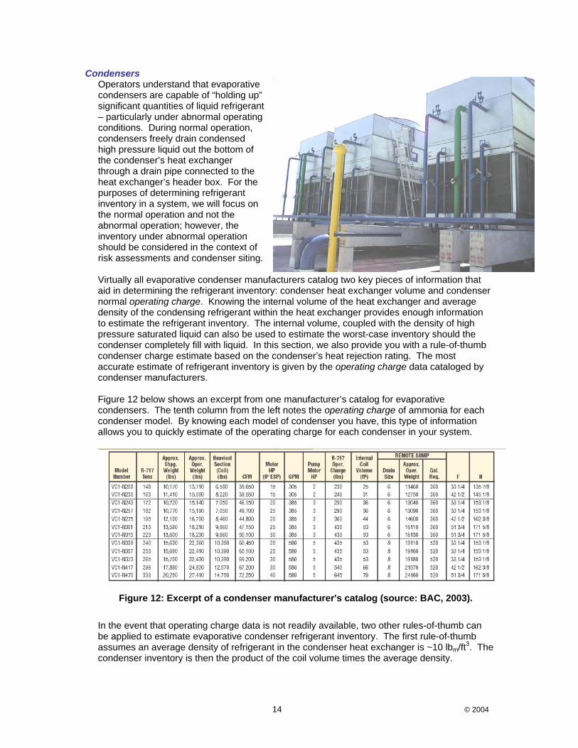
Condensers Operators understand that evaporative condensers are capable of “holding up” significant quantities of liquid refrigerant – particularly under abnormal operating conditions. During normal operation, condensers freely drain condensed high pressure liquid out the bottom of the condenser’s heat exchanger through a drain pipe connected to the heat exchanger’s header box. For the purposes of determining refrigerant inventory in a system, we will focus on the normal operation and not the abnormal operation; however, the inventory under abnormal operation should be considered in the context of risk assessments and condenser siting. Virtually all evaporative condenser manufacturers catalog two key pieces of information that aid in determining the refrigerant inventory: condenser heat exchanger volume and condenser normal operating charge. Knowing the internal volume of the heat exchanger and average density of the condensing refrigerant within the heat exchanger provides enough information to estimate the refrigerant inventory. The internal volume, coupled with the density of high pressure saturated liquid can also be used to estimate the worst-case inventory should the condenser completely fill with liquid. In this section, we also provide you with a rule-of-thumb condenser charge estimate based on the condenser’s heat rejection rating. The most accurate estimate of refrigerant inventory is given by the operating charge data cataloged by condenser manufacturers. Figure 12 below shows an excerpt from one manufacturer’s catalog for evaporative condensers. The tenth column from the left notes the operating charge of ammonia for each condenser model. By knowing each model of condenser you have, this type of information allows you to quickly estimate of the operating charge for each condenser in your system.
Figure 12: Excerpt of a condenser manufacturer's catalog (source: BAC, 2003).
In the event that operating charge data is not readily available, two other rules-of-thumb can be applied to estimate evaporative condenser refrigerant inventory. The first rule-of-thumb assumes an average density of refrigerant in the condenser heat exchanger is ~10 lbm/ft3. The condenser inventory is then the product of the coil volume times the average density.
15 © 2004
The second rule-of-thumb was developed based on evaluating operating charge data for a range of evaporative condenser types and sizes from which we concluded that a reasonable average charge is 90 lbm per million Btu/hr of rated heat rejection at a manufacturer’s-specified condition of 105°F saturated condensing and 70°F ambient wet-bulb temperature. In this case, the operating condenser operating charge can then be conservatively estimated by:
[ ] m,
lbmmBh 90mmBhref condenser nominalM Capacity≈ ⋅ (12)
If the rating of the condenser is expressed in “evaporator tons”, the corresponding rule-of-thumb is 1.85 lbm/evaporator ton (rated at 96.3°F saturated, 78°F wet-bulb and +20°F suction). Determining the maximum inventory of a condenser involves determining the density of liquid at the prevailing condensing pressure and multiplying that density by the cataloged condenser coil volume. Because the information provided by current condenser manufacturers is rather complete, rules-of-thumb need rarely be applied and condenser refrigerant inventory determination is straight forward.
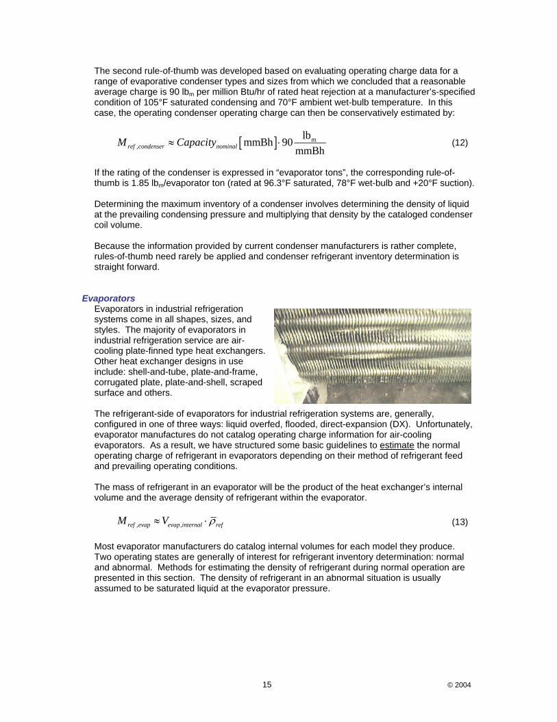
Evaporators Evaporators in industrial refrigeration systems come in all shapes, sizes, and styles. The majority of evaporators in industrial refrigeration service are air-cooling plate-finned type heat exchangers. Other heat exchanger designs in use include: shell-and-tube, plate-and-frame, corrugated plate, plate-and-shell, scraped surface and others. The refrigerant-side of evaporators for industrial refrigeration systems are, generally, configured in one of three ways: liquid overfed, flooded, direct-expansion (DX). Unfortunately, evaporator manufactures do not catalog operating charge information for air-cooling evaporators. As a result, we have structured some basic guidelines to estimate the normal operating charge of refrigerant in evaporators depending on their method of refrigerant feed and prevailing operating conditions.
The mass of refrigerant in an evaporator will be the product of the heat exchanger’s internal volume and the average density of refrigerant within the evaporator.
, ,ref evap evap internal refM V ρ≈ ⋅ (13) Most evaporator manufacturers do catalog internal volumes for each model they produce. Two operating states are generally of interest for refrigerant inventory determination: normal and abnormal. Methods for estimating the density of refrigerant during normal operation are presented in this section. The density of refrigerant in an abnormal situation is usually assumed to be saturated liquid at the evaporator pressure.

16 © 2004
Liquid Overfeed & Flooded Evaporators For liquid overfed and flooded evaporators, the average refrigerant density can be approximated by the following
( ), , , ,ref ref two phase outlet ref sat inCρ ρ ρ−≈ ⋅ + (14)
where refρ is the average refrigerant density in the coil (lbm/ft3), C is an empirical constant
(see table below), ρref,two-phase,outlet is the two-phase refrigerant density at the coil outlet, and ρref,sat,in is the density of saturated refrigerant liquid at the evaporator inlet. Estimates for the empirical constant are provided by the following table.
Table 1: Empirical constants for use in equation (14).
Refrigerant Feed C
Overfed 0.25
Flooded 0.5
The density of the two-phase refrigerant at the evaporator outlet is dependent on the quality of refrigerant at the coil outlet and the quality will be dependent on the liquid overfed ratio for the coil.
( )1
1x
OR=
+ (15)
where x is the mass fraction of vapor (i.e. quality) at the evaporator outlet and OR is the overfeed ratio (ratio of mass of liquid to mass of vapor leaving the evaporator). For liquid overfed evaporators, OR can be approximated by using the manufacturer’s-recommended overfeed rate for each evaporator. Alternatively, OR can be estimated by calculating the ratio of the liquid refrigerant supply flow rate to the evaporator over the minimum required flow rate just to meet the evaporator’s rated thermal performance. In this case, the liquid supply flow rate can be estimated based on the pressure difference across the hand-expansion valve and the valve’s Cv for the given number of turns open on the valve. For flooded evaporators, the OR is assumed to be 1. The specific volume of the mixed phase refrigerant out of the evaporator and corresponding density are given by
( ), ,
, ,
, ,
1
ref two phase outlet
ref two phase outlet
ref two phase outlet
liquid vapor liquidv v x v v
vρ
−
−
−
= + ⋅ −
=
(16)

17 © 2004
where x is quality, ρref,two-phase,outlet is the mixed phase density leaving the evaporator, vref,two-phase,outlet is the mixed phase specific volume leaving the evaporator, vvapor is the vapor specific volume and vliquid is the liquid phase specific volume both evaluated at saturation conditions for the pressure in the evaporator.
Direct-Expansion Evaporators For direct-expansion evaporators, the average density of refrigerant in the evaporator is:
( ), ,0.5ref ref inlet ref outletρ ρ ρ= ⋅ + (17)
where ρref,inlet is the density of refrigerant downstream of the expansion device and ρref,outlet is the refrigerant density at the outlet of the coil but upstream of any evaporator pressure regulator. The refrigerant density at the coil inlet is given by
( ), , ,,
1liquid inlet flash vapor inlet liquid inlet
ref inlet
v f v vρ
= + ⋅ − (18)
where fflash represents the flash gas (mass fraction of vapor) generated downstream of the expansion device. The flash gas fraction is calculated by
( )( )
,
, ,
high pressure liquid evapflash
vapor evap liquid evap
h hf
h h− −
=−
(19)
where hhigh-pressure is the enthalpy of high pressure liquid upstream of the expansion device, hliquid,evap is the enthalpy of saturated liquid at the evaporator pressure and hvapor,evap is the enthalpy of saturated vapor at the evaporator pressure.
For other evaporator types such as shell-and-tube chiller heat exchangers, manufacturers often provide operating charge data similar to that provided for condensers. As an example, Figure 13 shows a catalog sheet for a line of flooded shell-and-tube heat exchangers by one manufacturer. The seventh column from the left shows operating charge data for each chiller size. Because the volume of internal components in a chiller can vary significantly from manufacturer to manufacturer, we recommend that you contact the chiller manufacturer to obtain operating charge information for your particular model. In the absence of operating charge detailed data from the chiller manufacturer, a rule-of-thumb assumes the operating charge for a shell-and-tube chiller is 20 lbm per ton of refrigeration capacity per approach. Equation 20 includes an approximation for correcting the operating charge based on the design approach temperature for the chiller.
( )20
chillero
CapacityMT SET⋅
≈−
(20)
Where Capacity is the chiller capacity in tons, To is the design leaving fluid temperature from the chiller to the load [°F], and SET is the corresponding saturated evaporator temperature [°F] of the ammonia in the chiller. Welded (or nickel brazed) plate pair heat exchangers may be approximated using the methods for an air-cooling evaporator using the appropriate liquid feed type (gravity flooded or DX) with the volume determined by obtaining the volume of the refrigerant containing passages in the

18 © 2004
plate pair and the number of plate pairs. This information will require contact with the manufacturer of the plates.
Figure 13: Flooded shell-and-tube chiller data sheet (RVS).
19 © 2004
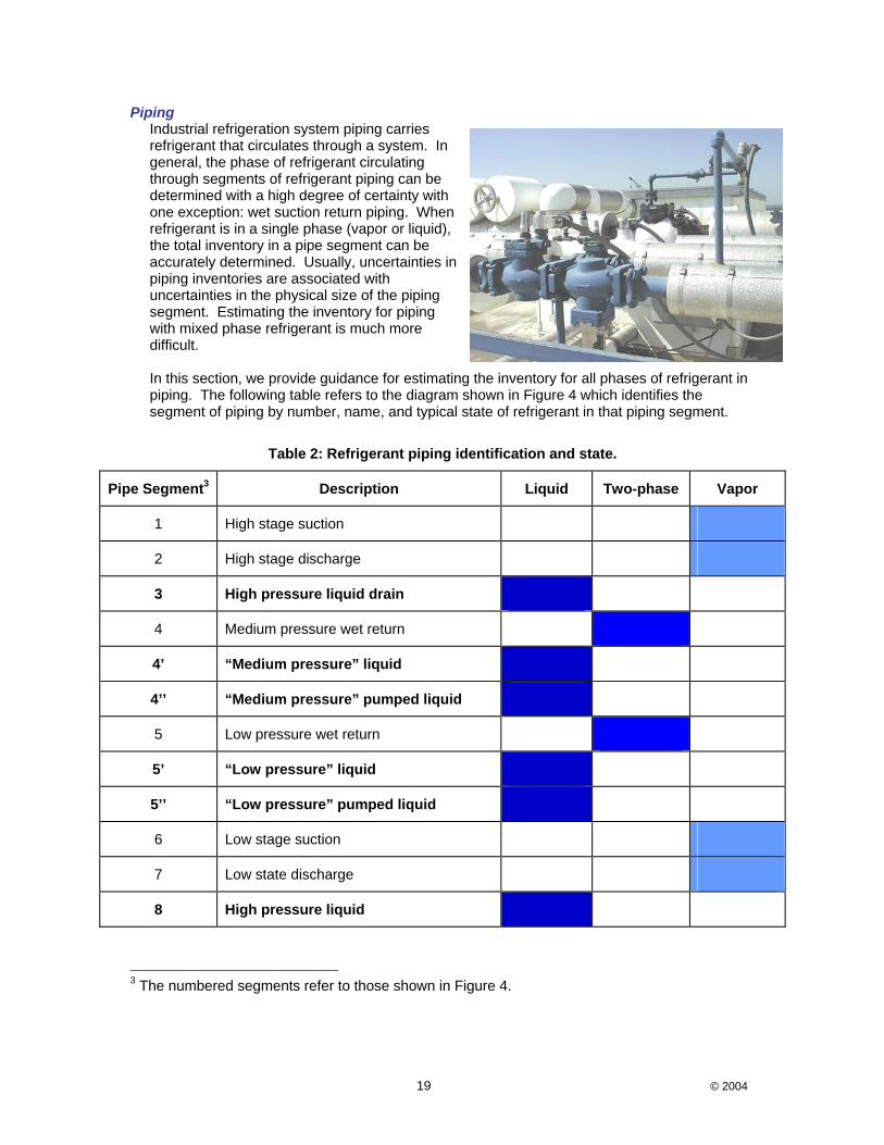
Piping Industrial refrigeration system piping carries refrigerant that circulates through a system. In general, the phase of refrigerant circulating through segments of refrigerant piping can be determined with a high degree of certainty with one exception: wet suction return piping. When refrigerant is in a single phase (vapor or liquid), the total inventory in a pipe segment can be accurately determined. Usually, uncertainties in piping inventories are associated with uncertainties in the physical size of the piping segment. Estimating the inventory for piping with mixed phase refrigerant is much more difficult. In this section, we provide guidance for estimating the inventory for all phases of refrigerant in piping. The following table refers to the diagram shown in Figure 4 which identifies the segment of piping by number, name, and typical state of refrigerant in that piping segment.
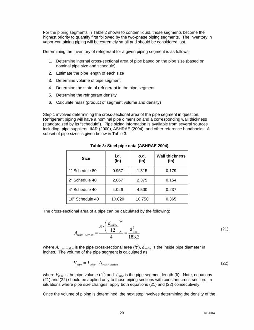
Table 2: Refrigerant piping identification and state.
Pipe Segment3 Description Liquid Two-phase Vapor
1 High stage suction
2 High stage discharge
3 High pressure liquid drain
4 Medium pressure wet return
4’ “Medium pressure” liquid
4’’ “Medium pressure” pumped liquid
5 Low pressure wet return
5’ “Low pressure” liquid
5’’ “Low pressure” pumped liquid
6 Low stage suction
7 Low state discharge
8 High pressure liquid
3 The numbered segments refer to those shown in Figure 4.
20 © 2004
For the piping segments in Table 2 shown to contain liquid, those segments become the highest priority to quantify first followed by the two-phase piping segments. The inventory in vapor-containing piping will be extremely small and should be considered last. Determining the inventory of refrigerant for a given piping segment is as follows:
1. Determine internal cross-sectional area of pipe based on the pipe size (based on nominal pipe size and schedule)
2. Estimate the pipe length of each size
3. Determine volume of pipe segment
4. Determine the state of refrigerant in the pipe segment
5. Determine the refrigerant density
6. Calculate mass (product of segment volume and density)
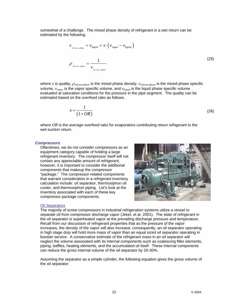
Step 1 involves determining the cross-sectional area of the pipe segment in question. Refrigerant piping will have a nominal pipe dimension and a corresponding wall thickness (standardized by its “schedule”). Pipe sizing information is available from several sources including: pipe suppliers, IIAR (2000), ASHRAE (2004), and other reference handbooks. A subset of pipe sizes is given below in Table 3.
Table 3: Steel pipe data (ASHRAE 2004).
Size i.d. (in)
o.d. (in)
Wall thickness (in)
1” Schedule 80 0.957 1.315 0.179
2” Schedule 40 2.067 2.375 0.154
4” Schedule 40 4.026 4.500 0.237
10” Schedule 40 10.020 10.750 0.365
The cross-sectional area of a pipe can be calculated by the following:
2
2124 183.3
inside
inside
cross section
dd
Aπ
−
⎛ ⎞⋅⎜ ⎟⎝ ⎠= =
(21)
where Across-section is the pipe cross-sectional area (ft2), dinside is the inside pipe diameter in inches. The volume of the pipe segment is calculated as
pipe pipe cross sectionV L A −= ⋅ (22)
where Vpipe is the pipe volume (ft3) and Lpipe is the pipe segment length (ft). Note, equations (21) and (22) should be applied only to those piping sections with constant cross-section. In situations where pipe size changes, apply both equations (21) and (22) consecutively. Once the volume of piping is determined, the next step involves determining the density of the

21 © 2004
refrigerant occupying each pipe segment. As previously discussed, the refrigerant density is dependent on the pressure and temperature of the refrigerant. Properties of ammonia are available from sources such as IRC (2001), ASHRAE (2001), and IIAR (1992). An excerpt from the IRC ammonia property tables is given below in Table 4. As an example, a high pressure liquid line with saturated liquid at 95ºF would be carrying refrigerant at a density of 36.67 lbm/ft3.
Table 4: Anhydrous ammonia properties at saturation conditions (IRC 2001).
The mass of refrigerant occupying the pipe segment is the product of the pipe segment volume (ft3) and the refrigerant density (lbm/ft3).
pipe pipe refrigerantM V ρ= ⋅ (23)
For liquid lines, the following correlation can be used to estimate the refrigerant inventory given inside pipe diameter and refrigerant saturation temperature.
2, ,
2
4.441 3.353 23.0282
0.2142 0.0002111 0.16767ref pipe est inside inside
sat sat inside sat
M d d
T T d T
= − ⋅ + ⋅
+ ⋅ − ⋅ − ⋅ ⋅ (24)
where Mref,pipe,est is the estimated mass (lbm) of liquid refrigerant per 100 ft of pipe, dinside is the inside diameter of the pipe (in), and Tsat is the liquid saturation temperature (°F). This correlation is valid for pipe sizes ranging from 1.5” – 2.5” (Schedule 80) and 3”-16” (Schedule 40). Applicable refrigerant temperatures range from: -40ºF to 100ºF (saturated liquid). The correlation yields an accuracy of -9.8% < Mref,pipe,est < 5% with an average error of 1%. For piping segments that carry two-phase flow, determining the mixed phase density becomes
22 © 2004
somewhat of a challenge. The mixed phase density of refrigerant in a wet return can be estimated by the following.
( ),
,
,
1
ref two phase
ref two phase
ref two phase
liquid vapor liquidv v x v v
vρ
−
−
−
= + ⋅ −
=
(25)
where x is quality, ρref,two-phase is the mixed phase density, vref,two-phase is the mixed phase specific volume, vvapor is the vapor specific volume, and vliquid is the liquid phase specific volume evaluated at saturation conditions for the pressure in the pipe segment. The quality can be estimated based on the overfeed ratio as follows.
( )1
1x
OR=
+ (26)
where OR is the average overfeed ratio for evaporators contributing return refrigerant to the wet-suction return.
Compressors
Oftentimes, we do not consider compressors as an equipment category capable of holding a large refrigerant inventory. The compressor itself will not contain any appreciable amount of refrigerant; however, it is important to consider the additional components that makeup the compressor “package.” The compressor-related components that warrant consideration in a refrigerant inventory calculation include: oil separator, thermosiphon oil cooler, and thermosiphon piping. Let’s look at the inventory associated with each of these key compressor package components. Oil Separators The majority of screw compressors in industrial refrigeration systems utilize a vessel to separate oil from compressor discharge vapor (Jekel, et al. 2001). The state of refrigerant in the oil separator is superheated vapor at the prevailing discharge pressure and temperature. Recall from our discussion of refrigerant properties that as the pressure of the vapor increases, the density of the vapor will also increase; consequently, an oil separator operating in high stage duty will hold more mass of vapor than an equal sized oil separator operating in booster service. A conservative estimate of the refrigerant mass in an oil separator will neglect the volume associated with its internal components such as coalescing filter elements, piping, baffles, heating elements, and the accumulated oil itself. These internal components can reduce the gross internal volume of the oil separator by 20-30%. Assuming the separator as a simple cylinder, the following equation gives the gross volume of the oil separator:
23 © 2004
2
, 4separator
oil separator cylinder
DV Lπ= ⋅ ⋅ (27)
The mass of refrigerant vapor in the separator can be conservatively estimated using:
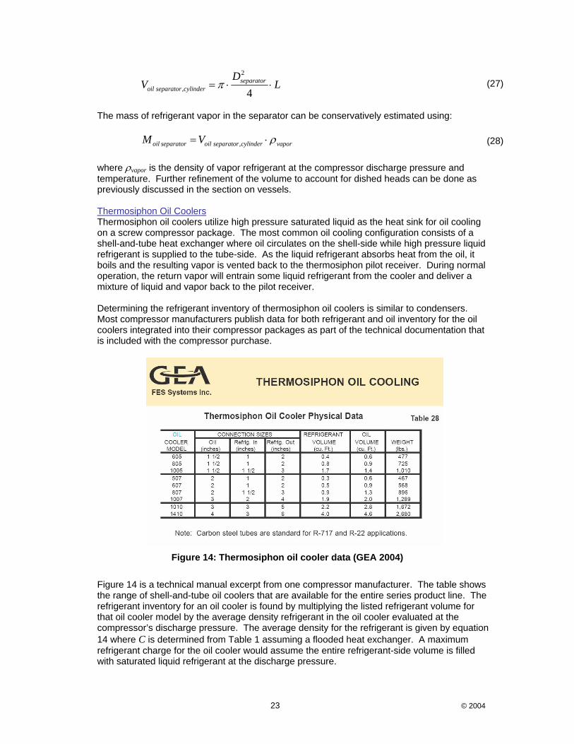
,oil separator oil separator cylinder vaporM V ρ= ⋅ (28) where ρvapor is the density of vapor refrigerant at the compressor discharge pressure and temperature. Further refinement of the volume to account for dished heads can be done as previously discussed in the section on vessels. Thermosiphon Oil Coolers Thermosiphon oil coolers utilize high pressure saturated liquid as the heat sink for oil cooling on a screw compressor package. The most common oil cooling configuration consists of a shell-and-tube heat exchanger where oil circulates on the shell-side while high pressure liquid refrigerant is supplied to the tube-side. As the liquid refrigerant absorbs heat from the oil, it boils and the resulting vapor is vented back to the thermosiphon pilot receiver. During normal operation, the return vapor will entrain some liquid refrigerant from the cooler and deliver a mixture of liquid and vapor back to the pilot receiver. Determining the refrigerant inventory of thermosiphon oil coolers is similar to condensers. Most compressor manufacturers publish data for both refrigerant and oil inventory for the oil coolers integrated into their compressor packages as part of the technical documentation that is included with the compressor purchase.
Figure 14: Thermosiphon oil cooler data (GEA 2004)
Figure 14 is a technical manual excerpt from one compressor manufacturer. The table shows the range of shell-and-tube oil coolers that are available for the entire series product line. The refrigerant inventory for an oil cooler is found by multiplying the listed refrigerant volume for that oil cooler model by the average density refrigerant in the oil cooler evaluated at the compressor’s discharge pressure. The average density for the refrigerant is given by equation 14 where C is determined from Table 1 assuming a flooded heat exchanger. A maximum refrigerant charge for the oil cooler would assume the entire refrigerant-side volume is filled with saturated liquid refrigerant at the discharge pressure.
24 © 2004
For a high stage compressor, saturated liquid ammonia at 181 psig has a density of 36.67 lbm/ft3. The maximum refrigerant inventory for a model 6074 oil cooler would then be the product of the listed refrigerant volume (0.5 ft3) and the refrigerant density (36.67 lbm/ft3) resulting in an estimated operating charge of 33.34 lbm. Recently, plate-type heat exchangers have found growing application for thermosiphon oil cooling. An primary advantage of the plate-type heat exchanger is its compact size (which leads to low operating charge) for a given oil cooling load. For example, a flat plate-type heat exchanger capable of rejecting 881 mBh of oil cooling load has a refrigerant-side internal volume of approximately 0.2 ft3. If we assumed that the oil cooler in this example was completely filled with saturated liquid at a design condensing temperature (181 psig), the refrigerant charge would be just over 7 lbm (the product of 0.2 ft3 and the refrigerant density of 36.67 lbm/ft3). Thermosiphon Piping The methods presented in the piping portion of this TechNote should be applied to estimate inventory of thermosiphon piping. The refrigerant state in the thermosiphon supply piping will be saturated liquid while the thermosiphon return piping will contain a mixture of liquid and vapor. The refrigerant inventory for the thermosiphon supply piping can be estimated using equations (21)-(23) or equation (24). The refrigerant inventory for thermosiphon return piping can be estimated by equations (21)-(23) where the refrigerant density for equation (23) is estimated using equations (25)-(26). Typically, the ratio of liquid mass to vapor mass in the return piping is 3:1 (FES, 1998 and Welch, 2003); consequently, a value for OR in equation (26) can be assumed to be 3 for inventory estimating purposes.
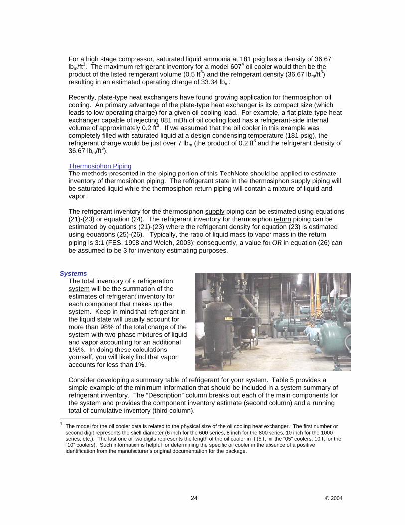
Systems
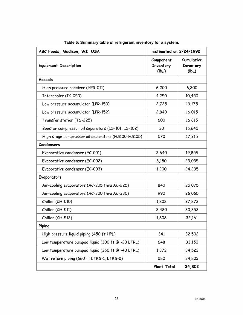
The total inventory of a refrigeration system will be the summation of the estimates of refrigerant inventory for each component that makes up the system. Keep in mind that refrigerant in the liquid state will usually account for more than 98% of the total charge of the system with two-phase mixtures of liquid and vapor accounting for an additional 1½%. In doing these calculations yourself, you will likely find that vapor accounts for less than 1%. Consider developing a summary table of refrigerant for your system. Table 5 provides a simple example of the minimum information that should be included in a system summary of refrigerant inventory. The “Description” column breaks out each of the main components for the system and provides the component inventory estimate (second column) and a running total of cumulative inventory (third column).
4 The model for the oil cooler data is related to the physical size of the oil cooling heat exchanger. The first number or
second digit represents the shell diameter (6 inch for the 600 series, 8 inch for the 800 series, 10 inch for the 1000 series, etc.). The last one or two digits represents the length of the oil cooler in ft (5 ft for the “05” coolers, 10 ft for the “10” coolers). Such information is helpful for determining the specific oil cooler in the absence of a positive identification from the manufacturer’s original documentation for the package.
25 © 2004
Table 5: Summary table of refrigerant inventory for a system.
ABC Foods, Madison, WI USA Estimated on 2/24/1992
Equipment Description Component Inventory
(lbm)
Cumulative Inventory
(lbm)
Vessels
High pressure receiver (HPR-011) 6,200 6,200
Intercooler (IC-050) 4,250 10,450
Low pressure accumulator (LPR-150) 2,725 13,175
Low pressure accumulator (LPR-152) 2,840 16,015
Transfer station (TS-225) 600 16,615
Booster compressor oil separators (LS-101, LS-102) 30 16,645
High stage compressor oil separators (HS100-HS105) 570 17,215
Condensers
Evaporative condenser (EC-001) 2,640 19,855
Evaporative condenser (EC-002) 3,180 23,035
Evaporative condenser (EC-003) 1,200 24,235
Evaporators
Air-cooling evaporators (AC-205 thru AC-225) 840 25,075
Air-cooling evaporators (AC-300 thru AC-330) 990 26,065
Chiller (CH-510) 1,808 27,873
Chiller (CH-511) 2,480 30,353
Chiller (CH-512) 1,808 32,161
Piping
High pressure liquid piping (450 ft HPL) 341 32,502
Low temperature pumped liquid (300 ft @ -20 LTRL) 648 33,150
Low temperature pumped liquid (360 ft @ -40 LTRL) 1,372 34,522
Wet return piping (660 ft LTRS-1, LTRS-2) 280 34,802
Plant Total 34,802
26 © 2004
Conclusion Accurately estimating the refrigerant charge in a system is the first step in determining whether or not your plant falls within the scope of OSHA’s Process Safety Management Standard and EPA’s Risk Management Program. For ammonia refrigeration systems having inventories in excess of the threshold quantity (10,000 lbm), end-users are required to develop and implement both a process safety management and risk management program. The process safety information portion of the PSM Standard requires maintaining up-to-date information on the inventory of a refrigeration system. Component level inventories also provide useful data for other facets of safety such as evaluating risk through a formal process hazard analysis. If you are unsure of applying the inventory calculation methods presented in this TechNote, work through some of the example problems provided in the Appendix. Check the IRC website for computer-aided tools that will assist you in rapidly estimating the refrigerant inventory for components in a refrigeration system.
27 © 2004
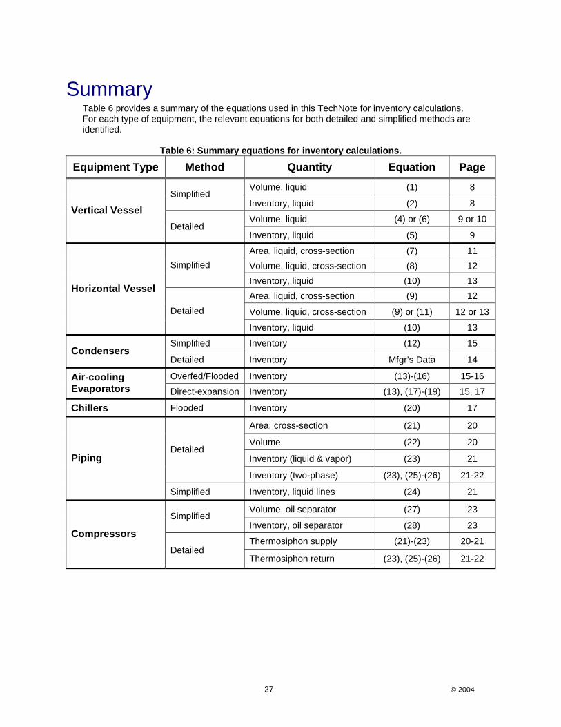
Summary Table 6 provides a summary of the equations used in this TechNote for inventory calculations. For each type of equipment, the relevant equations for both detailed and simplified methods are identified.
Table 6: Summary equations for inventory calculations.
Equipment Type Method Quantity Equation Page
Volume, liquid (1) 8 Simplified
Inventory, liquid (2) 8
Volume, liquid (4) or (6) 9 or 10 Vertical Vessel
Detailed Inventory, liquid (5) 9
Area, liquid, cross-section (7) 11 Volume, liquid, cross-section (8) 12 Simplified
Inventory, liquid (10) 13 Area, liquid, cross-section (9) 12
Volume, liquid, cross-section (9) or (11) 12 or 13
Horizontal Vessel
Detailed
Inventory, liquid (10) 13
Simplified Inventory (12) 15 Condensers
Detailed Inventory Mfgr’s Data 14
Overfed/Flooded Inventory (13)-(16) 15-16 Air-cooling Evaporators Direct-expansion Inventory (13), (17)-(19) 15, 17
Chillers Flooded Inventory (20) 17
Area, cross-section (21) 20
Volume (22) 20
Inventory (liquid & vapor) (23) 21 Detailed
Inventory (two-phase) (23), (25)-(26) 21-22
Piping
Simplified Inventory, liquid lines (24) 21
Volume, oil separator (27) 23 Simplified
Inventory, oil separator (28) 23
Thermosiphon supply (21)-(23) 20-21 Compressors
Detailed Thermosiphon return (23), (25)-(26) 21-22
28 © 2004
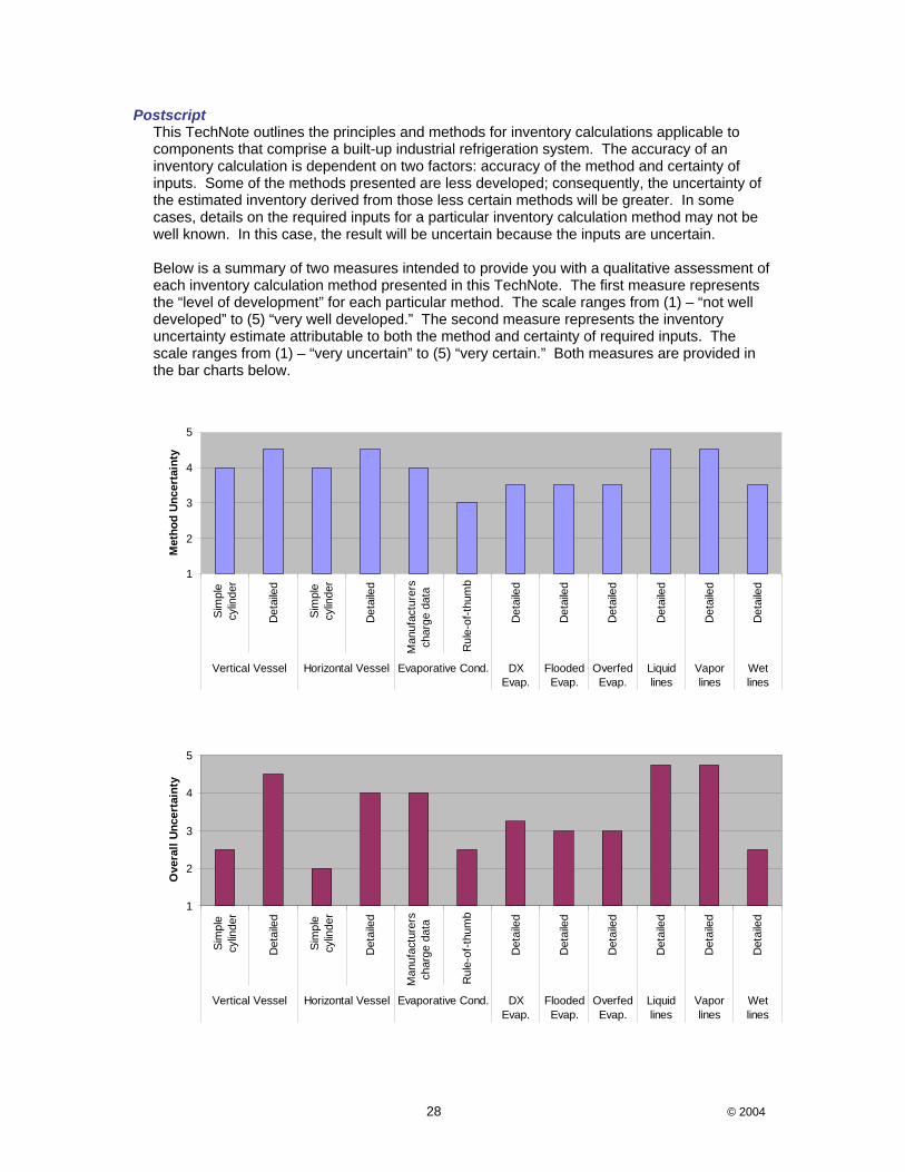
Postscript This TechNote outlines the principles and methods for inventory calculations applicable to components that comprise a built-up industrial refrigeration system. The accuracy of an inventory calculation is dependent on two factors: accuracy of the method and certainty of inputs. Some of the methods presented are less developed; consequently, the uncertainty of the estimated inventory derived from those less certain methods will be greater. In some cases, details on the required inputs for a particular inventory calculation method may not be well known. In this case, the result will be uncertain because the inputs are uncertain. Below is a summary of two measures intended to provide you with a qualitative assessment of each inventory calculation method presented in this TechNote. The first measure represents the “level of development” for each particular method. The scale ranges from (1) – “not well developed” to (5) “very well developed.” The second measure represents the inventory uncertainty estimate attributable to both the method and certainty of required inputs. The scale ranges from (1) – “very uncertain” to (5) “very certain.” Both measures are provided in the bar charts below.
1
2
3
4
5
Sim
ple
cylin
der
Det
aile
d
Sim
ple
cylin
der
Det
aile
d
Man
ufac
ture
rsch
arge
dat
a
Rul
e-of
-thum
b
Det
aile
d
Det
aile
d
Det
aile
d
Det
aile
d
Det
aile
d
Det
aile
d
Vertical Vessel Horizontal Vessel Evaporative Cond. DXEvap.
FloodedEvap.
OverfedEvap.
Liquidlines
Vaporlines
Wetlines
Met
hod
Unc
erta
inty
1
2
3
4
5
Sim
ple
cylin
der
Det
aile
d
Sim
ple
cylin
der
Det
aile
d
Man
ufac
ture
rsch
arge
dat
a
Rul
e-of
-thum
b
Det
aile
d
Det
aile
d
Det
aile
d
Det
aile
d
Det
aile
d
Det
aile
d
Vertical Vessel Horizontal Vessel Evaporative Cond. DXEvap.
FloodedEvap.
OverfedEvap.
Liquidlines
Vaporlines
Wetlines
Ove
rall
Unc
erta
inty
29 © 2004
References ASHRAE, HVAC Systems and Equipment Handbook, American Society of Heating, Refrigerating,
and Air conditioning Engineers, Atlanta, GA (2004). ASHRAE, Fundamentals Handbook, American Society of Heating, Refrigerating, and Air
conditioning Engineers, Atlanta, GA (2001). BAC, “Series V Evaporative Condensers”, Baltimore Aircoil, Bulletin S119/1-OB (2003). IIAR, Ammonia Refrigeration Piping Handbook, International Institute of Ammonia Refrigeration,
Arlington, VA, (2000). EPA, “Compliance Guidance for Industrial Process Refrigeration Leak Repair Regulations Under
Section 608 of the Clean Air Act”, www.epa.gov/ozone/title6/608/compguid/guidance.pdf, (1995).
EPA, “Risk Management Program”, 40 CFR Part 68, Accidental Release Prevention
Requirements: Risk Management Programs Under the Clean Air Act, Section 112(r)(7), June 20, 1996.
FES, “S Series Screw Compressor Technical Manual”, Bulletin 209(S)-TM, February (1998). GEA, Excerpted from the FES compressor Technical Manual, personal communication, (2004). IIAR, Ammonia Data Book, International Institute of Ammonia Refrigeration, Arlington, VA (1992). IRC, “Ammonia Properties Spreadsheet”, Industrial Refrigeration Consortium at the University of
Wisconsin-Madison, Madison, WI, http://www.irc.wisc.edu/software/, (2000). Jekel, T. B., Reindl, D. T., and Fisher, J. M., “Gravity Separator Fundamentals and Design”, IIAR
Proceedings, Long Beach Meeting, March (2001). OSHA, “Process Safety Management of Highly Hazardous Chemicals”, 29 CFR 1910.119, Final
Rule; Federal Register Vol. 57, No. 36, pp. 6356-6417, February 24, 1992. RVS, “Refrigeration Heat Exchangers”, brochure (chiller information reference) undated. Welch, J., “Thermosiphon System Design”, Proceedings of the International Institute of Ammonia
Refrigeration, Albuquerque, pp. 283-313, (2003).

30 © 2004
Appendix: Examples

31 © 2004
Vessels Determine the mass of refrigerant in a -40 F pumped recirculator that measures 8 ft in diameter and 12 ft high. Liquid refrigerant is maintained at the 4 ft level during normal operation. Assume the vessel is a vertical cylinder and estimate the refrigerant inventory associated with both the liquid and vapor. Solution:
The volume of liquid is given by
2 238 4 201 ft
4 4vessel
liquid liquiddV Hπ π= ⋅ = ⋅ =
The density of saturated liquid at -40ºF is 43.08 lbm/ft3; consequently, the mass of liquid in the vessel is
3m43.08 201 ft 8,659 lbliquidM = ⋅ =
The volume of vapor is given by
2 238 8 402 ft
4 4vessel
vapor vapordV Hπ π= ⋅ = ⋅ =
32 © 2004
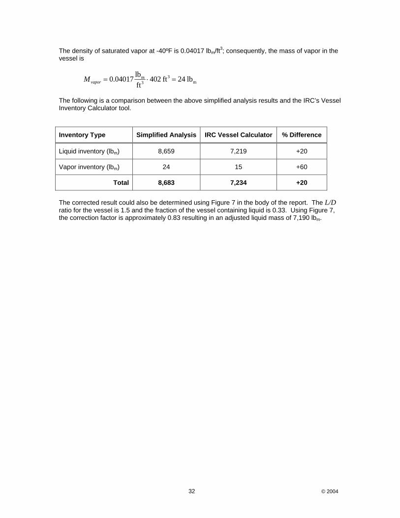
The density of saturated vapor at -40ºF is 0.04017 lbm/ft3; consequently, the mass of vapor in the vessel is
3mm3
lb0.04017 402 ft 24 lbftvaporM = ⋅ =
The following is a comparison between the above simplified analysis results and the IRC’s Vessel Inventory Calculator tool.
Inventory Type Simplified Analysis IRC Vessel Calculator % Difference
Liquid inventory (lbm) 8,659 7,219 +20
Vapor inventory (lbm) 24 15 +60
Total 8,683 7,234 +20
The corrected result could also be determined using Figure 7 in the body of the report. The L/D ratio for the vessel is 1.5 and the fraction of the vessel containing liquid is 0.33. Using Figure 7, the correction factor is approximately 0.83 resulting in an adjusted liquid mass of 7,190 lbm.

33 © 2004
Condensers Determine the refrigerant inventory for an Evapco ATC Model 3459B. Solution: The table below is an excerpt from Evapco’s evaporative condenser product data catalog. From the entry showing the model 3459B, we find the reported operating charge of 4,780 lbm.
This particular condenser has a nominal capacity of 50,848 mBh. Applying the rule-of-thumb of 90 lbm/mmBh yields an estimated operating charge of
mm
lb mmBh90 50,848 mBh 4,576 lbmmBh 1,000 mBhestM = ⋅ ⋅ =
The last rule-of-thumb we introduced suggested taking the reported internal coil volume and using an average density of lbm/ft3. With this rule-of-thumb, the estimated inventory would be
3 m
,2 m3lb532ft 10 5,320 lbftestM = ⋅ =
34 © 2004
Evaporator Estimate the inventory for an overfed evaporator operating with a -20ºF liquid supply and a 3:1 overfeed ratio. The coil does not have an evaporator pressure regulator. The internal volume is 4 ft3. Solution: The density of liquid at -20ºF is 42.23 lbm/ft3 and the corresponding specific volume is 0.0237 ft3/lbm. The density of vapor at -20ºF is 0.06809 lbm/ft3 and the corresponding specific volume is 14.686 ft3/lbm. The first step is to estimate the quality of refrigerant at the evaporator outlet, x.
( ) ( ),1 1 0.25
1 1 3evap outletxoverfeed
= = =+ +
Next, we estimate the specific volume and density of refrigerant at the coil outlet
( )3
, ,m
m, , 3
, ,
ft0.0237 0.25 14.686 0.0237 3.689lb
1 1 lb0.27113.689 ft
ref two phase outlet
ref two phase outletref two phase outlet
v
vρ
−
−−
= + − =
= = =
The average density of refrigerant in the coil can now be estimated
( )( )
, , , ,
m3
lb0.25 0.2711 42.23 10.6ft
ref ref two phase outlet ref sat inCρ ρ ρ−= ⋅ +
= ⋅ + =
Finally, we have enough information to estimate the refrigerant inventory for the coil
3 m, , m3
lb4 ft 10.6 42.5 lbftref evap evap internal refM V ρ= ⋅ = ⋅ =
35 © 2004
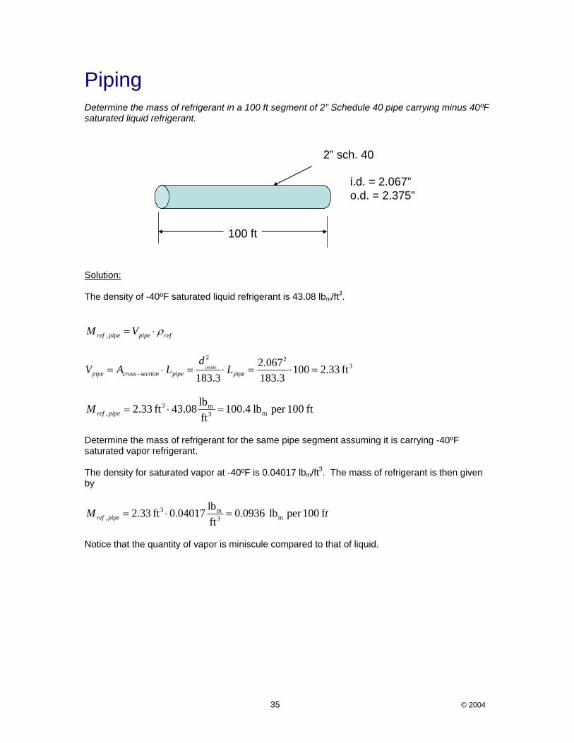
Piping Determine the mass of refrigerant in a 100 ft segment of 2” Schedule 40 pipe carrying minus 40ºF saturated liquid refrigerant.
100 ft
2” sch. 40
i.d. = 2.067”o.d. = 2.375”
Solution: The density of -40ºF saturated liquid refrigerant is 43.08 lbm/ft3.
,ref pipe pipe refM V ρ= ⋅
2 232.067 100 2.33 ft
183.3 183.3inside
pipe cross section pipe pipe
dV A L L−= ⋅ = ⋅ = ⋅ =
3 m
, m3
lb2.33 ft 43.08 100.4 lb per 100 ftftref pipeM = ⋅ =
Determine the mass of refrigerant for the same pipe segment assuming it is carrying -40ºF saturated vapor refrigerant. The density for saturated vapor at -40ºF is 0.04017 lbm/ft3. The mass of refrigerant is then given by
3 m, m3
lb2.33 ft 0.04017 0.0936 lb per 100 fftref pipeM t= ⋅ =
Notice that the quantity of vapor is miniscule compared to that of liquid.
36 © 2004
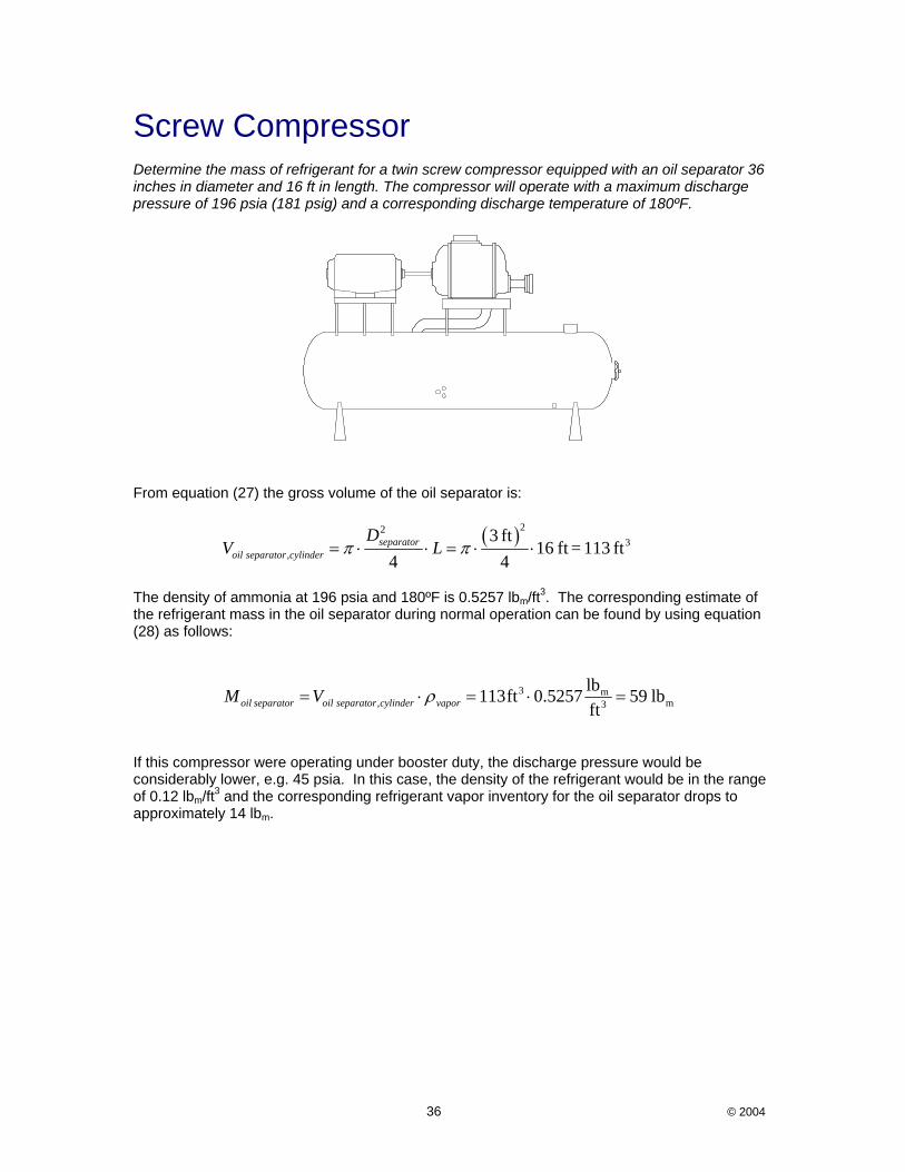
Screw Compressor Determine the mass of refrigerant for a twin screw compressor equipped with an oil separator 36 inches in diameter and 16 ft in length. The compressor will operate with a maximum discharge pressure of 196 psia (181 psig) and a corresponding discharge temperature of 180ºF. From equation (27) the gross volume of the oil separator is:
( )223
,
3 ft16 ft = 113 ft
4 4separator
oil separator cylinder
DV Lπ π= ⋅ ⋅ = ⋅ ⋅
The density of ammonia at 196 psia and 180ºF is 0.5257 lbm/ft3. The corresponding estimate of the refrigerant mass in the oil separator during normal operation can be found by using equation (28) as follows:
3 m, m3
lb113ft 0.5257 59 lbftoil separator oil separator cylinder vaporM V ρ= ⋅ = ⋅ =
If this compressor were operating under booster duty, the discharge pressure would be considerably lower, e.g. 45 psia. In this case, the density of the refrigerant would be in the range of 0.12 lbm/ft3 and the corresponding refrigerant vapor inventory for the oil separator drops to approximately 14 lbm.