Refined thresholds for nonlinear ground motion and temporal

Geophys. J. Int. (2010) doi: 10.1111/j.1365-246X.2010.04704.x

GJI

Sei

smol

ogy

Refined thresholds for non-linear ground motion and temporalchanges of site response associated with medium-size earthquakes

Chunquan Wu,1 Zhigang Peng1 and Yehuda Ben-Zion2

1School of Earth and Atmospheric Sciences, Georgia Institute of Technology, Atlanta, GA 30332, USA. E-mail: [email protected] of Earth Sciences, University of Southern California, Los Angeles, CA 90089-0740, USA

Accepted 2010 June 15. Received 2010 June 15; in original form 2010 February 22

S U M M A R YWe systematically analyse non-linear effects and temporal changes of site response associatedwith medium-size earthquakes, using seismic data recorded by the Japanese Strong MotionNetwork KIK-Net. We apply a sliding-window spectral ratio technique to surface and boreholestrong motion records at six sites, and stack results associated with different earthquakes thatproduce similar peak ground acceleration (PGA). In some cases we observe a weak coseismicdrop in the peak frequency when the PGA is as small as ∼20–30 Gal, and near instantaneousrecovery after the passage of the direct S waves. The percentage of drop in the peak frequencystarts to increase with increasing PGA values. We also observe a coseismic drop in the peakspectral ratio for two sites. When the PGA is larger than ∼60 Gal to more than 100 Gal, weobserve considerably stronger drops of the peak frequencies followed by logarithmic recoverywith time. The observed weak reductions of peak frequencies with near instantaneous recoverylikely reflect non-linear response with essentially fixed level of damage, while the larger dropsfollowed by logarithmic recovery reflect the generation (and then recovery) of additional rockdamage. The results indicate clearly that non-linear site response may occur during medium-size earthquakes, and that the PGA threshold for in situ non-linear behaviour is lower than thepreviously thought value of ∼100–200 Gal.

Key words: Elasticity and anelasticity; Earthquake ground motions; Site effects; Wave prop-agation.

1 I N T RO D U C T I O N

Non-linear site response is associated with deviations from the lineartrend predicted by Hooke’s elasticity when the amplitude of groundmotion exceeds a certain threshold. This phenomenon is well docu-mented in both laboratory experiments (Ostrovsky & Johnson 2001,and references within) and under in situ conditions (Beresnev & Wen1996, and references within). Generally, non-linear response has astrong correlation with the level of ground motion (e.g. Hartzell1998; Su et al. 1998; Johnson et al. 2009) along with rock typeand other characteristics of the sites (e.g. Beresnev & Wen 1996;Hartzell 1998; Trifunac et al. 1999; Tsuda et al. 2006). Quantifi-cation of soil non-linearity and subsequent consequences for siteresponse are currently key components of estimating seismic haz-ard, predicting future ground motions (Frankel et al. 2000) anddesigning geotechnical and structural engineering systems on soils(NEHRP 2003).

Comparisons of the site response during strong and weak groundmotions provide one of the most typical ways to identify non-linearsite behaviour. Several recent studies have also investigated detailsof the recovery process from non-linear response by computingthe temporal evolution of spectral ratios between a target site anda nearby reference site (e.g. Pavlenko & Irikura 2002; Sawazakiet al. 2006; Karabulut & Bouchon 2007; Sawazaki et al. 2009; Wu

et al. 2009a, b; Rubinstein 2010). These studies generally identifystrong reductions of peak frequencies (i.e. resonant frequencies)measured in the spectral ratios during the strong ground motionsof a nearby large earthquake, followed by logarithmic recoveriesto the level before the large event. The timescales of the recov-eries observed in these studies are quite different. In some cases,the coseismic changes appear to recover on timescales of min-utes or less (e.g. Pavlenko & Irikura 2002; Karabulut & Bouchon2007), while in other cases the recoveries appear to last foryears (e.g. Sawazaki et al. 2006). Some of the documented dif-ferences may stem from different analysis resolutions, but theymay also reflect (at least partially) different types of non-linearbehaviour.

Lyakhovsky et al. (2009) analysed theoretically the response of asolid governed by a non-linear damage rheology and highlighted theexistence of two forms of non-linear behaviour. With fixed existingmaterial damage, the non-linear effects are small and the recoveryto linear behaviour with reduction of source amplitude is instanta-neous. When the source motion leads to increasing material damage,the non-linear effects are considerably larger and the recovery to lin-ear behaviour after the source ceases to operate is logarithmic withtime. Both forms of non-linear response of materials to loading areseen clearly in high-resolution laboratory experiments (Pasqualiniet al. 2007).

C© 2010 The Authors 1Journal compilation C© 2010 RAS

Geophysical Journal International

2 Wu et al.

Because non-linear effects tend to be clear particularly understrong shaking, most of the previous observational seismologicalstudies on this topic focused on large earthquakes (typically largerthan Mw = 6). They found that non-linear site response typicallymanifests beyond an amplitude threshold of 100–200 Gal or dy-namic strain of 10−5 to 10−4 (e.g. Beresnev & Wen 1996). On theother hand, laboratory studies identified non-linear effects for geo-materials under strains as small as 10−8 (TenCate et al. 2004). Usingrepeating earthquakes, Rubinstein & Beroza (2004) found reduc-tion of S-wave velocities in the near surface (which could be usedas a proxy for resonant frequency) after an Mw = 5.4 aftershock ofthe 1989 Mw = 6.9 Loma Prieta earthquake. Recently, Rubinstein(2010) used the spectral ratio method to analyse strong groundmotion recordings of 13 earthquakes with magnitudes of 3.7–6.5(including the 2003 Mw = 6.5 San Simeon earthquake, 2004 Mw =6.0 Parkfield earthquake and their aftershocks). He found that atthe Turkey Flat site, ∼35 Gal of peak ground acceleration (PGA)produces non-linear site effects, suggesting that non-linear effectscould be much more common than previously thought.

In a previous study (Wu et al. 2009a), we quantified the effects ofthe input ground motion on the degree of non-linearity by applyingthe spectral ratio method to the strong motion data recorded by apair of surface and borehole stations before, during and after the2004 Mw = 6.8 mid-Niigata earthquake sequence. We found thatthe coseismic peak frequency reduction and the post-seismic re-covery time increase with the peak ground velocity (PGV) beyond∼5 cm s−1, or PGA beyond ∼100 Gal. We were unable to iden-tify clear coseismic drop and post-seismic recovery with PGA lessthan 100 Gal, mainly because of averaging effects associated withthe employed 10-s sliding window. We noted that by reducing thesliding-window size to smaller values, it may be possible to detectmore subtle non-linear site response associated with smaller inputground motions.

In this work, we apply the sliding-window spectral ratio methodwith a small window size to the strong motion data generated by∼2000 medium-size earthquakes recorded by six pairs of surfaceand borehole stations (Fig. 1). These include the data analysed pre-viously by Wu et al. (2009a), together with a few sites that haveshown non-linear responses by other recent studies (Sawazaki et al.2006, 2009; Assimaki et al. 2008). Because we have more than2000 seismic records, we are able to stack the spectral ratios forcorresponding PGA values, which result in stable measurements.Our analysis shows that the peak frequency starts to decrease atPGA levels of several tens of Gal, followed in some cases by a nearinstantaneous recovery. When the PGA values exceed ∼60 Galto more than 100 Gal, the onset of non-linear response is fol-lowed by a gradual recovery. The two different observed formsof non-linear behaviour for different ranges of excitation levels areconsistent with the theoretical expectations based on the damagemodel of Lyakhovsky et al. (2009) and the laboratory observationsof Pasqualini et al. (2007). The low thresholds for the onset of insitu non-linear effects, documented in this work and the study ofRubinstein (2010), imply that non-linear models should be consid-ered for smaller earthquakes than previously thought (e.g. Kramer& Paulsen 2004).

2 DATA A N D A NA LY S I S P RO C E D U R E

2.1 Seismic data

The analysis employs strong motion data recorded by six stations(MYGH04, NIGH06, NIGH12, SMNH01, IWTH04 and IWTH05)

in the Japanese Digital Strong-Motion Seismograph Network KiK-Net operated by the National Research Institute for Earth Scienceand Disaster Prevention (Aoi et al. 2000). The network consistsof 659 stations with an uphole/downhole pair of strong-motionseismometers. Each KiK-Net unit consists of three-component ac-celerometers and a data logger having a 24-bit analogue-to-digitalconverter with a sampling frequency of 200 Hz.

The six stations used in this study are chosen mainly becauseprevious studies have identified clear non-linear effects at these sta-tions during large events (Sawazaki et al. 2006; Assimaki et al. 2008;Sawazaki et al. 2009;Wu et al. 2009a). We also find that the observedtemporal changes in peak frequencies and peak spectral ratios (max-imum of the spectral ratios) at these stations are much clearer thanthose at other stations, allowing us to better detect potential temporalchanges associated with relatively small ground motions. Additionaldetails on the network and site conditions can be found in Table S1,Fig. S1 (see the Supporting Information section for both), or at theKiK-Net website (http://www.kik.bosai.go.jp/kik/index_en.shtml).

In the subsequent analysis we utilize a total of 2204 events thatoccurred between 1999 January and 2008 May and recorded by thesix surface and borehole strong motion sensors (see also Table S2).The magnitudes of most events range from 3 to 5, and the hypocen-tral depths range from 5 to 70 km. The recorded PGAs of mostevents range from 0 to 100 Gal, generally less than the 100–200 Galthreshold for non-linear site effects suggested by previous studies(e.g. Chin & Aki 1991; Beresnev & Wen 1996).

2.2 Analysis procedure

The analysis procedure follows overall those of Sawazaki et al.(2006, 2009) and Wu et al. (2009a). The main analysis steps are asfollows: we use 6-s time windows that are moved forward by 2 s forall waveforms recorded by the surface and borehole stations. Thezero time corresponds to the hand-picked S-wave arrival, and weuse the time corresponding to starting point of each window todenote the time of that window. In such case, the window corre-sponding to the S-arrival window (i.e. zero time) fully captures thestrongest motion during the S-wave. We have tested various windowlengths and sliding values. Our testing results indicate, as noted byWu et al. (2009a), that increasing window length would miss thetemporal changes over small timescales. On the other hand, de-creasing window length would reduce the stability of the results.The employed 6-s window appears to be a well-balanced value forthe examined data between temporal resolution and stability. Allpossible seismic phases, including pre-event noise, P, S and codawaves are analysed together. Next, we remove the mean value ofthe traces and apply a 5 per cent Hanning taper to both ends. Wecompute the Fourier power spectra of the two horizontal compo-nents and take the square root of the sum to get the amplitude ofthe vector sum of the two horizontal spectra. The obtained spectraare smoothed by applying the mean smoothing algorithm from thesubroutine ‘smooth’ in the Seismic Analysis Code (Goldstein et al.2003), with half width of 0.5 Hz. We tested different smoothingwindow sizes, and found that smoothing window with half width of0.5 Hz could remove most of the noisy spikes while not changingthe overall shape of spectra significantly. The spectral ratios areobtained by dividing the combined horizontal spectra of surfacestations by the spectra of the borehole stations.

Fig. 2 shows an example of the original acceleration records atNIGH06 generated by an M 5.3 event on 2004 October 25 and the6-s windows used to compute the spectral ratios for the direct S and

C© 2010 The Authors, GJI

Journal compilation C© 2010 RAS

Non-linear site response by medium-size events 3

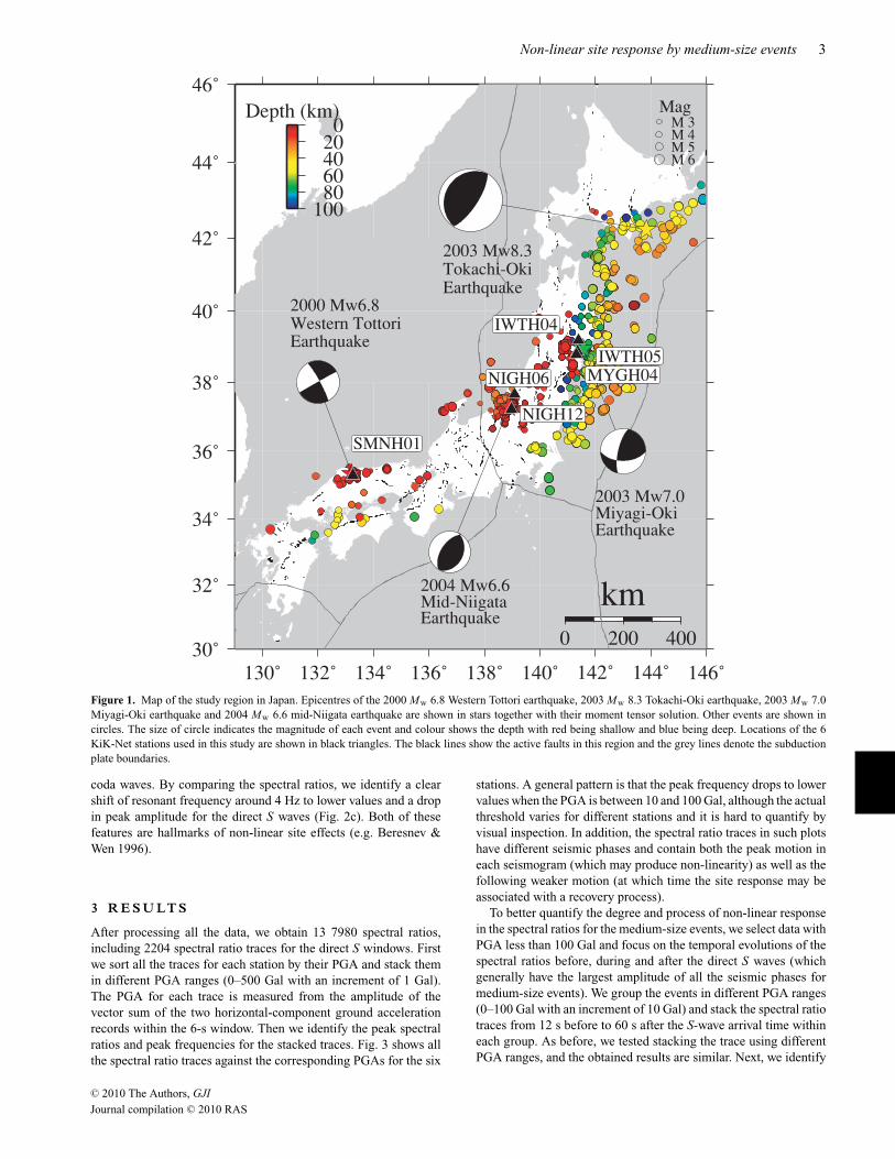
Figure 1. Map of the study region in Japan. Epicentres of the 2000 Mw 6.8 Western Tottori earthquake, 2003 Mw 8.3 Tokachi-Oki earthquake, 2003 Mw 7.0Miyagi-Oki earthquake and 2004 Mw 6.6 mid-Niigata earthquake are shown in stars together with their moment tensor solution. Other events are shown incircles. The size of circle indicates the magnitude of each event and colour shows the depth with red being shallow and blue being deep. Locations of the 6KiK-Net stations used in this study are shown in black triangles. The black lines show the active faults in this region and the grey lines denote the subductionplate boundaries.

coda waves. By comparing the spectral ratios, we identify a clearshift of resonant frequency around 4 Hz to lower values and a dropin peak amplitude for the direct S waves (Fig. 2c). Both of thesefeatures are hallmarks of non-linear site effects (e.g. Beresnev &Wen 1996).

3 R E S U LT S

After processing all the data, we obtain 13 7980 spectral ratios,including 2204 spectral ratio traces for the direct S windows. Firstwe sort all the traces for each station by their PGA and stack themin different PGA ranges (0–500 Gal with an increment of 1 Gal).The PGA for each trace is measured from the amplitude of thevector sum of the two horizontal-component ground accelerationrecords within the 6-s window. Then we identify the peak spectralratios and peak frequencies for the stacked traces. Fig. 3 shows allthe spectral ratio traces against the corresponding PGAs for the six

stations. A general pattern is that the peak frequency drops to lowervalues when the PGA is between 10 and 100 Gal, although the actualthreshold varies for different stations and it is hard to quantify byvisual inspection. In addition, the spectral ratio traces in such plotshave different seismic phases and contain both the peak motion ineach seismogram (which may produce non-linearity) as well as thefollowing weaker motion (at which time the site response may beassociated with a recovery process).

To better quantify the degree and process of non-linear responsein the spectral ratios for the medium-size events, we select data withPGA less than 100 Gal and focus on the temporal evolutions of thespectral ratios before, during and after the direct S waves (whichgenerally have the largest amplitude of all the seismic phases formedium-size events). We group the events in different PGA ranges(0–100 Gal with an increment of 10 Gal) and stack the spectral ratiotraces from 12 s before to 60 s after the S-wave arrival time withineach group. As before, we tested stacking the trace using differentPGA ranges, and the obtained results are similar. Next, we identify



4 Wu et al.

Figure 2. (a) East-component ground accelerations recorded at the station NIGH06 generated by an M 5.3 earthquake on 2004 October 25. Surface recordingis shown at the top and borehole recording is shown at the bottom. The red and blue dashed lines indicate the direct S and coda window that are used to computethe acceleration spectra in (b) and spectral ratios in (c).

Figure 3. Stacked spectral ratios from all the 6-s windows plotted against PGA for the six stations (a–f). All the spectral ratio traces for each station arestacked based on the PGA of each sliding window from 0 to 1000 Gal with a step of 1 Gal. The x-axis shows the PGA value in log scale, and the y-axis showsthe frequency. The spectral ratio value are colour-coded with red being high and blue being low. Gaps represent no data. The horizontal dashed lines indicatethe resonance frequencies without non-linearity measured from 0–10 Gal.

the peak spectral ratio and peak frequency for the stacked trace ineach PGA range. Fig. 4 illustrates the procedure for data recordedat site NIGH06. The results show again a sudden drop of peakspectral ratio and a shift of the spectral peak to lower frequencies

during the S-wave arrival, and these changes become clear whenthe PGA exceeds certain threshold. Similar analyses using dataat the other sites indicate that the threshold varies from ∼20 to∼80 Gal among the different stations, and the degree of




Figure 4. Stacked spectral ratios for station NIGH06 plotted against the traveltime relative to the S-wave arrival. Spectral ratio traces from 12 s before to 60 safter the S-wave arrival are stacked based on the PGA of that event from 0 to 100 Gal with a step of 10 Gal (a–j). We also include the results between 100–200 Gal and >200 Gal for comparison (k–l). The spectral ratio value are colour-coded with red being high and blue being low. The PGA range and number ofthe stacked events are marked at the left- and right-hand side on the top of each panel. The horizontal dashed lines indicate the reference resonance frequencyof 4.4 Hz.

non-linearity (i.e. percentage drop of peak frequency) also variesfor different stations.

Using the obtained results, we examine the relationship betweenthe observed temporal changes and the input ground motion, byrelating the percentage of drop in peak frequency and peak spectralratio with the PGA range for the stacked traces. We use the measuredpeak frequency and peak spectral ratio for the stacked trace in thePGA range 0–10 Gal as the reference values. To test the validityof the reference value, we have compared the stacked spectral ratiotrace in the PGA range of 0–10 Gal with those traces from low-amplitude coda-windows, and found that they are nearly identical(Fig. 5a). We also checked individual spectral ratio traces in thePGA range of 0–10 Gal, and found no significant variation in peakfrequency (Fig. 5b).

We calculate the percentage reduction for both peak frequencyand peak spectral ratio associated with the S waves, by comparingthe 6-s windows immediately after the S-wave arrivals with thereference values. The peak frequency drop (PFD) and peak spectralratio drop (PSRD) are defined by

PFD = ( fr − fs)/

fr , (1)

PSRD = (PSRr − PSRs)/

PSRr , (2)

where fr and PSRr are the reference peak frequency and peak spec-tral ratio, respectively, and fs and PSRs are the peak frequency andpeak spectral ratio measured at the 6-s window immediately afterthe S-wave arrival, respectively. Because the degree of non-linearityis site specific, we use 10 per cent of the PFD or PSRD measured



6 Wu et al.

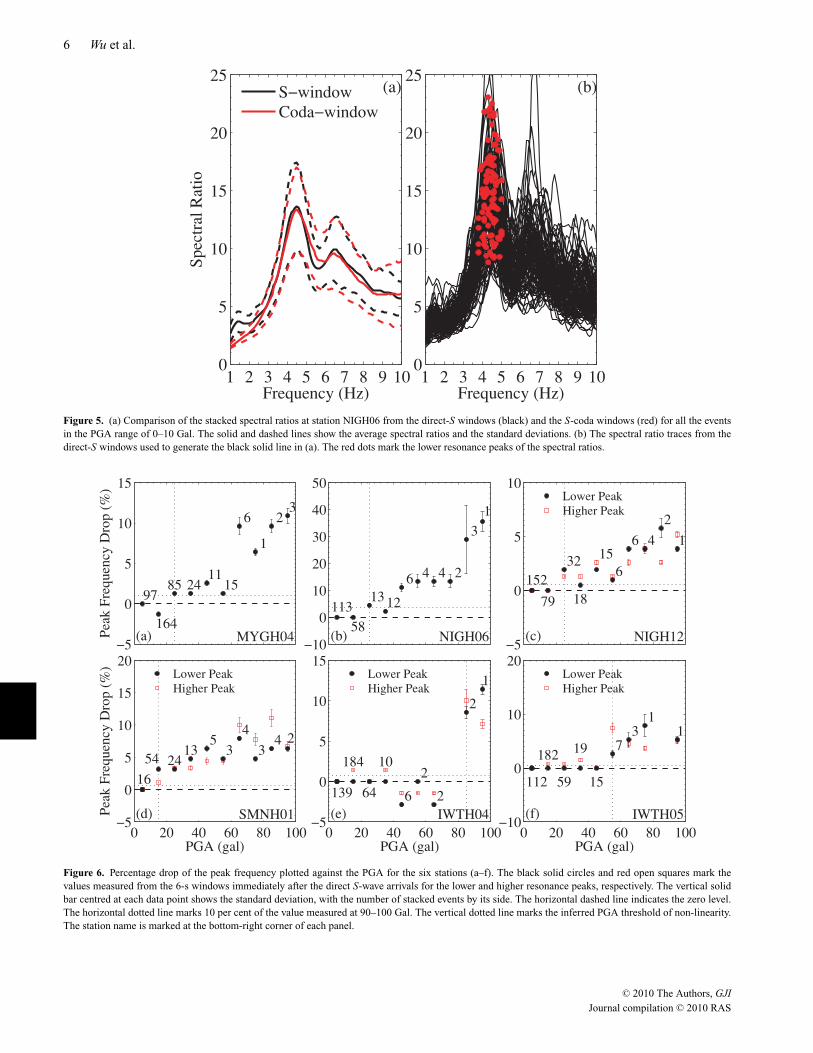
Figure 5. (a) Comparison of the stacked spectral ratios at station NIGH06 from the direct-S windows (black) and the S-coda windows (red) for all the eventsin the PGA range of 0–10 Gal. The solid and dashed lines show the average spectral ratios and the standard deviations. (b) The spectral ratio traces from thedirect-S windows used to generate the black solid line in (a). The red dots mark the lower resonance peaks of the spectral ratios.

Figure 6. Percentage drop of the peak frequency plotted against the PGA for the six stations (a–f). The black solid circles and red open squares mark thevalues measured from the 6-s windows immediately after the direct S-wave arrivals for the lower and higher resonance peaks, respectively. The vertical solidbar centred at each data point shows the standard deviation, with the number of stacked events by its side. The horizontal dashed line indicates the zero level.The horizontal dotted line marks 10 per cent of the value measured at 90–100 Gal. The vertical dotted line marks the inferred PGA threshold of non-linearity.The station name is marked at the bottom-right corner of each panel.




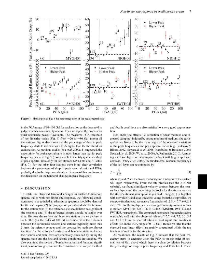
Figure 7. Similar plot as Fig. 6 for percentage drop of the peak spectral ratio.

in the PGA range of 90–100 Gal for each station as the threshold tojudge whether non-linearity occurs. Then we repeat the process forother resonance peaks if available. The measured PGA thresholdof non-linearity varies (Fig. 6) from ∼20 to ∼80 Gal among allthe stations. Fig. 6 also shows that the percentage of drop in peakfrequency starts to increase with PGA higher than the threshold foreach station. As previous studies (Wu et al. 2009a, b) suggested, theuncertainty for peak spectral ratio is much larger than that for peakfrequency (see also Fig. 5b). We are able to identify systematic dropof peak spectral ratio only for two stations MYGH04 and NIGH06(Fig. 7). For the other four stations there is no clear correlationbetween the percentage of drop in peak spectral ratio and PGA,probably due to the large uncertainties. Because of this, we focus inthe discussion on the temporal changes in peak frequency.

4 D I S C U S S I O N

To relate the observed temporal changes in surface-to-boreholespectral ratios with non-linear site response, the following condi-tions need to be satisfied: (1) the source spectrum should be identicalfor the station pair; (2) the propagation path should also be the samefor the station pair; (3) the reference site should have no significantsite response and (4) the reference spectra should be stable overtime. Because the surface and borehole stations are very close toeach other (on the order of 100 m) as compared to the distancesbetween the earthquake sources and stations (typically more than5 km), the seismic sources and the propagation path are almostidentical for the colocated surface and borehole stations. Hencetheir source and path terms are effectively cancelled by taking thespectral ratio and the first and second conditions are satisfied. Wealso examined the spectra of borehole stations and found no signif-icant peaks or troughs, and no clear variation over time, so the third

and fourth conditions are also satisfied to a very good approxima-tion.

Non-linear site effects (i.e. reduction of shear modulus and in-creased damping) induced by strong motions of medium-size earth-quakes are likely to be the main origin of the observed variationsin the peak frequencies and peak spectral ratios (e.g. Pavlenko &Irikura 2002; Sawazaki et al. 2006; Karabulut & Bouchon 2007;Sawazaki et al. 2009; Wu et al. 2009a, b; Rubinstein 2010). Assum-ing a soft soil layer over a half-space bedrock with large impedancecontrast (Dobry et al. 2000), the fundamental resonant frequency fof the soil layer can be computed by

f = Vs

4H, (3)

where Vs and H are the S-wave velocity and thickness of the surfacesoil layer, respectively. From the site profiles (see the KiK-Netwebsite), we found significant velocity contrast between the near-surface layers and the underlying bedrocks for the six stations, sothe aforementioned assumption is justified. Using eq. (3), togetherwith the velocity and layer thickness values from the site profiles, wecompute fundamental resonance frequencies of 13.8, 4, 7.7, 6.6, 2.8and 3.2 Hz for the top layers where strongest velocity contrast occursat stations MYGH04, NIGH06, NIGH12, SMNH01, IWTH04 andIWTH05, respectively. The computed resonance frequencies agreereasonably well with the observed values of 15.7, 4.4, 7.7, 6.3, 3.5and 3.8 Hz from the spectral ratios without significant non-lineareffects (i.e. in the PGA range of 0–10 Gal). Hence we infer that theobserved non-linear effects are mainly constrained within the topfew tens of metres for the six sites.

As mentioned, the results of Fig. 6 indicate that the peak fre-quency starts to decrease when the PGA is on the order of sev-eral tens of Gal, above which there is a clear correlation betweenthe percentage of drop in peak frequency and PGA level. These



8 Wu et al.

Figure 8. (a) Percentage drop of the peak frequency measured from 10-s windows plotted against the PGA at NIGH06 from Wu et al. (2009a). The solidcircles mark the values measured from the 10-s windows immediately after the direct S-wave arrivals. The vertical solid bar centred at each data point showsthe standard deviation. The horizontal dashed line indicates the pre-mainshock value. The vertical grey dotted line marks the PGA value of 100 Gal. (b) Similarplot as (a) for 6-s windows. Values below 100 Gal are measured from the stacked spectral ratio traces (Fig. 6b), and values above 100 Gal are measured fromindividual even. The horizontal dotted line marks 10 per cent of the value measured at 90–100 Gal. The vertical dotted line marks the inferred PGA thresholdof non-linearity.

observations, together with the results of previous studies (e.g.Hartzell 1998; Su et al. 1998; Johnson et al. 2009; Wu et al. 2009a),support the view that non-linear effects strongly correlate with thelevel of ground motion. However, the ∼20–30 Gal PGA thresholdrevealed by our analysis is lower than the value of 100–200 Galfound by most previous studies (e.g. Beresnev & Wen 1996). Thisis perhaps not too surprising, because as far as we know none ofthe previous studies except the recent work by Rubinstein (2010)investigated non-linear site effects with PGA less than 100 Gal (typ-ically associated with medium-size events). The non-linear effectswith PGA less than 100 Gal are generally much weaker than thetraditional non-linear site effects associated with stronger shaking(Fig. 8b). Since most previous studies mainly focused on individualevents (rather than stacked data), the subtle non-linear effects arequite likely to be buried by low signal-to-noise ratio (SNR). Fromthe comparison of our results (Fig. 8b) with the results of Wu et al.(2009a) without stacking (Fig. 8a), we could see a clearer image ofthe PFD in the PGA range of 0–100 Gal after stacking. Hence, thestacking technique utilized in this study helps to reveal the other-wise buried small non-linear effects in a statistical way. However,stacking requires a significant amount of strong motion recordings,which was not available until the last decade. In addition, reducingthe sliding-window size from 10 to 6 s helps to identify subtle co-seismic changes associated only with the direct S waves, which alsocauses some differences in the results for PGA > 100 Gal (Fig. 8).

The PFDs found in this study for PGA < 100 Gal are typicallywithin the duration of the S wave (e.g. Fig. 4). In some cases (e.g.60–70, 70–80 and 90–100 > 200 Gal), we can identify the log-arithmic type of recovery found by various previous studies (e.g.Sawazaki et al. 2006; Wu et al. 2009a). However, such recovery isnot clear in other cases with lower PGA values. One possible expla-nation is that the observed weak non-linear effects are induced indamaged rocks by increasing wave amplitude without causing ad-ditional material damage. This is consistent with the analytical andnumerical results of Lyakhovsky et al. (2009) for a continuum non-linear damage rheology model. The results from that study showa few percentage shift in the resonance frequency with increasingground motion at a constant damage level, and tens of percent-age shift in the resonance frequency with increasing damage level.These two forms of non-linear effects are observed clearly in thelaboratory experiments of Pasqualini et al. (2007).

Based on the results of Fig. 6, the percentage of drop in peakfrequency is generally very small (<5 per cent) at the onset ofnon-linearity, except for station IWTH04. At this station, the pointbetween 60 and 70 Gal is missing, which may blur the true picture.When the PGA value is approaching 100 Gal, the percentage dropat station NIGH06 could be as large as 35 per cent. Therefore,when the PGA level is relatively low the ground motion is probablynot strong enough to cause additional damage to the medium. Inthis case weak non-linear effects with increasing ground motion formaterial with frozen damage level or very minor additional damageis likely to be the major mechanism for our observations. On theother hand, when the PGA level is relatively high (i.e. approachingor large than 100 Gal), additional damage is generated and we startto observe much larger changes in the peak frequency (Fig. 8),followed by logarithmic recovery (Fig. 4). We have tried to quantifythe recovery timescale for the coseismic PFD (see Wu et al. 2009afor additional analysis details). However, because the coseismicdrop in peak frequency is small (Fig. 6, especially for lower PGAranges), and the logarithmic recovery on short timescales is veryfast (Fig. 4), we were not able to identify a sharp boundary betweenthe near instantaneous recovery and the rapid logarithmic recovery.Based on the stacked spectral ratios for the six sites (e.g. Fig. 4),the higher PGA threshold for production of significant additionaldamage and considerably stronger non-linear effects (i.e. tens ofpercentage drop in peak frequency followed by a clear logarithmictype of recovery) ranges from ∼60 Gal to more than 100 Gal.

We note that higher pre-existing damage makes the medium moresusceptible to further damage, since it is generally easier to nucleateand grow cracks in material with higher crack density. Rubinstein& Beroza (2004) and Rubinstein (2010) used the correlation be-tween pre-exiting damage and susceptibility to additional damageto explain non-linear effects associated with increasing damage in-duced by M 4–5.5 aftershocks of the 1989 Mw 6.9 Loma Prietaearthquake and 2004 Mw 6.0 Parkfield earthquake. Here we attemptto resolve non-linear response that is not associated with furtherincrease of the damage. We believe this is the situation in the caseswith near instantaneous recovery to linear behaviour in the timeswindows after the direct S waves for the following two reasons.First, we examined the damage recovery time of both large andsmall earthquakes utilized in this study and by Wu et al. (2009a)and found that the maximum recovery time to 90 per cent of the




reference value is less than 200 s. Since most aftershocks occurredwell beyond this time interval, most of the damage caused by thepreceding large earthquakes has been recovered at the occurrencetime of each earthquake we utilized, and is continuously decreas-ing further. Some low-amplitude damage remains for longer du-rations, as documented in studies with repeating earthquakes (e.g.Rubinstein & Beroza 2004; Peng & Ben-Zion 2006), and contributesto the overall long-term damage evident by the lower seismic ve-locities in the near surface material and fault zone structures (e.g.Li et al. 1990; Peng et al. 2003; Liu et al. 2005; Lewis & Ben-Zion 2010). Such remaining and decreasing transient damage willproduce some apparent non-zero recovery time of the non-linear be-haviour. However, this damage was produced by the previous eventsrather than by the motion that generates the subtle non-linear effectswe observe. Second, we also identified weak non-linear effects formedium-size earthquakes before the M >6 events in each site, andwe found no clear change in the non-linear response for medium-size earthquakes before and after large events. Hence, we concludethat some of the non-linear effects we observe for the medium-sizeearthquakes reflect non-linear response of damaged rocks withoutadditional increments to the levels of damage.

According to Fig. 6, the PGA onset and degree of non-linearityappear to vary significantly at different sites, so the PGA thresh-old probably also depends on the site conditions. We examinedthe site conditions in terms of the site classification by the aver-age S-wave velocity (VS30) in the upper 30 m of the site (NEHRP2003), soil types at the top layers of each site and the S-wavevelocity contrast, but none of these properties shows any clear cor-relation with the PGA onset (see Table S1). It is likely that theexisting rock damage at each site controls the onset of non-linearity(e.g. Lyakhovsky et al. 2009). A useful quantification of the near-surface damage layer is the crack density, which could be estimatedfrom analyses of seismic scattering and shear wave splitting (e.g.Revenaugh 2000; Liu et al. 2005; Chao & Peng 2009). However,such analyses are beyond the scope of this paper. In any case, theresults obtained in this study, together with the recent work of Rubin-stein (2010), suggest that non-linear site response can be induced bymedium-size (M 4–5) earthquakes and can occur more commonlythan previously thought. The observed weak form of non-linearitywith near instantaneous recovery is likely associated with near con-stant material damage. As noted before, laboratory studies haveidentified non-linear effects for geomaterials under strains as smallas 10−8 (TenCate et al. 2004), which is much smaller than the dy-namic strains (10−6–10−5) induced by the earthquakes utilized inthis study. Observing non-linear effects associated with such weakmotion under in situ conditions will require the development of ad-ditional analysis techniques and high resolution data. Although thesignificance of weak non-linearity is case specific, quantification ofnon-linearity at different degrees will help to further advance ourunderstanding of site response to shaking caused by earthquakes.

A C K N OW L E D G M E N T S

We thank the National Research Institute for Earth Science andDisaster Prevention (NIED) for providing us with the strong mo-tion records of KiK-Net. We thank Reiji Kobayashi for providingthe knet2sac program to convert original k-net data format intoSAC format, and Wei Li for helping with the data download andinsightful discussions. The study was funded by the National Sci-ence Foundation (grant EAR-0908310) and the Southern CaliforniaEarthquake Center (based on NSF Cooperative Agreement EAR-0106924 and USGS Cooperative Agreement 02HQAG0008). The

paper benefited from comments by two anonymous referees andEditor Massimo Cocco.

R E F E R E N C E S

Aoi, S., Obara, K., Hori, S., Kasahara, K. & Okada, Y., 2000. New Japaneseuphole/downhole strong-motion observation network: KiK-net, Seism.Res. Lett, 72, 239.

Assimaki, D., Li, W., Steidl, J. & Tsuda, K., 2008. Site amplification and at-tenuation via downhole array seismogram inversion: a comparative studyof the 2003 Miyagi-Oki aftershock sequence, Bull. seism. Soc. Am., 98,301–330.

Beresnev, I. & Wen, K., 1996. Nonlinear soil response - A reality?, Bull.seism. Soc. Am., 86, 1964–1978.

Chao, K. & Peng, Z., 2009. Temporal changes of seismic velocity andanisotropy in the shallow crust induced by the 1999 October 22 M6. 4Chia-Yi, Taiwan earthquake, Geophys. J. Int., 179, 1800–1816.

Chin, B. & Aki, K., 1991. Simultaneous study of the source, path, and siteeffects on strong ground motion during the 1989 Loma Prieta earthquake:a preliminary result on pervasive nonlinear site effects, Bull. seism. Soc.Am., 81, 1859–1884.

Dobry, R., et al. 2000. New site coefficients and site classification systemused in recent building seismic code provisions, Earthq. Spectra, 16,41–67.

Frankel, A., et al. 2000. USGS national seismic hazard Maps, Earthq. Spec-tra, 16, 1–19.

Goldstein, P., Dodge, D., Firpo, M. & Minner, L., 2003. SAC2000: sig-nal processing and analysis tools for seismologists and engineers. in TheIASPEI International Handbook of Earthquake and Engineering Seis-mology, Part B, Chap 85.5, eds Lee, W.H.K., Kanamori, H., Jennings, P.C. & Kisslinger, C., Academic Press, London.

Hartzell, S., 1998. Variability in nonlinear sediment response during the1994 Northridge, California, earthquake, Bull. seism. Soc. Am., 88,1426–1437.

Johnson, P., Bodin, P., Gomberg, J., Pearce, F., Lawrence, Z. & Menq, F.,2009. Inducing in situ, nonlinear soil response applying an active source,J. geophys. Res., 114, B05304, doi:10.1029/2008JB005832.

Karabulut, H. & Bouchon, M., 2007. Spatial variability and non-linearity of strong ground motion near a fault, Geophys. J. Int., 170,262–274.

Kramer, S. & Paulsen, S., 2004. Practical use of geotechnical site responsemodels, 10, in Proceedings of International Workshop on Uncertaintiesin Nonlinear Soil Properties and their Impact on Modeling Dynamic SoilResponse, University of California, Berkeley.

Lewis, M.A. & Ben-Zion, Y., 2010. Diversity of fault zone damage andtrapping structures in the Parkfield section of the San Andreas Faultfrom comprehensive analysis of near fault seismograms, Geophys. J. Int.,submitted.

Li, Y., Leary, P., Aki, K. & Malin, P., 1990. Seismic trapped modes in theOroville and San Andreas fault zones, Science, 249, 763–766.

Liu, Y., Teng, T. & Ben-Zion, Y., 2005. Near-surface seismic anisotropy,attenuation and dispersion in the aftershock region of the 1999 Chi-Chiearthquake, Geophys. J. Int., 160, 695–706.

Lyakhovsky, V., Hamiel, Y., Ampuero, J. & Ben-Zion, Y., 2009. Non-lineardamage rheology and wave resonance in rocks, Geophys. J. Int., 178,910–920.

NEHRP, 2003, NEHRP Recommended Provisions for Seismic Regulationsfor New Buildings and Other Structures (FEMA 450), National Earth-quake Hazards Reduction Program (NEHRP), Building Seismic SafetyCouncil, Washington, DC.

Ostrovsky, L. & Johnson, P., 2001. Dynamic nonlinear elasticity in geoma-terials, Rivista del Nuovo Cimento, 24, 1–46.

Pasqualini, D., Heitmann, K., TenCate, J., Habib, S., Higdon, D. &Johnson, P., 2007. Nonequilibrium and nonlinear dynamics in Bereaand Fontainebleau sandstones: low-strain regime, J. geophys. Res, 112,B01204, doi:01210.01029/02006JB004264.



10 Wu et al.

Pavlenko, O. & Irikura, K., 2002. Nonlinearity in the response of soils inthe 1995 Kobe earthquake in vertical components of records, Soil. Dyn.Earthq. Eng., 22, 967–975.

Peng, Z. & Ben-Zion, Y., 2006. Temporal changes of shallow seismic veloc-ity around the Karadere-Duzce branch of the north Anatolian Fault andstrong ground motion, Pure appl. Geophys., 163, 567–600.

Peng, Z., Ben-Zion, Y., Michael, A. & Zhu, L., 2003. Quantitative analysisof seismic fault zone waves in the rupture zone of the 1992 Landers, Cal-ifornia, earthquake: evidence for a shallow trapping structure, Geophys.J. Int., 155, 1021–1041.

Revenaugh, J., 2000. The relation of crustal scattering to seismicity in South-ern California, J. geophys. Res., 105, 25403–25422.

Rubinstein, J., 2010. Nonlinear strong ground motion in medium magnitudeearthquakes near Parkfield, CA, Bull. seism. Soc. Am., submitted.

Rubinstein, J. & Beroza, G., 2004. Nonlinear strong ground motion in theML 5.4 Chittenden earthquake: Evidence that preexisting damage in-creases susceptibility to further damage, Geophys. Res. Lett, 31, L23614,doi:23610.21029/22004GL021357.

Sawazaki, K., Sato, H., Nakahara, H. & Nishimura, T., 2006. Temporalchange in site response caused by earthquake strong motion as revealedfrom coda spectral ratio measurement, Geophys. Res. Lett., 33, L21303,doi:21310.21029/22006GL027938.

Sawazaki, K., Sato, H., Nakahara, H. & Nishimura, T., 2009. Time-lapsechanges of seismic velocity in the shallow ground caused by strong groundmotion shock of the 2000 Western-Tottori earthquake, Japan, as revealedfrom coda deconvolution analysis, Bull. seism. Soc. Am., 99, 352–366.

Su, F., Anderson, J. & Zeng, Y., 1998. Study of weak and strong ground mo-tion including nonlinearity from the Northridge, California, earthquakesequence, Bull. seism. Soc. Am., 88, 1411–1425.

TenCate, J., Pasqualini, D., Habib, S., Heitmann, K., Higdon, D. & Johnson,P., 2004. Nonlinear and nonequilibrium dynamics in geomaterials, Phys.Rev. Lett., 93, doi:10.1103/PhysRevLett.1193.065501.

Trifunac, M., Hao, T. & Todorovska, M., 1999. On the reoccurrence of sitespecific response, Soil. Dyn. Earthq. Eng., 18, 569–592.

Tsuda, K., Archuleta, R. & Jamison, S., 2006. Confirmation of nonlinearsite response: case study from 2003 and 2005 Miyagi-Oki earthquakes,Bull. seism. Soc. Am., 96, 926–942.

Wu, C., Peng, Z. & Assimaki, D., 2009a. Temporal changes in site re-sponse associated with strong ground motion of 2004 Mw6. 6 mid-Niigata earthquake sequences in Japan, Bull. seism. Soc. Am., 99, 3487–3495.

Wu, C., Peng, Z. & Ben-Zion, Y., 2009b. Non-linearity and temporal changesof fault zone site response associated with strong ground motion, Geo-phys. J. Int., 176, 265–278.

S U P P O RT I N G I N F O R M AT I O N

Additional Supporting Information may be found in the online ver-sion of this article:

Tables with site and event information.Table S1. Station locations, and the site conditions including VS30

(m s−1), site classification, max VS constrast, soil types and non-linearity threshold (Gal) for the six sites.Table S2. List of the information of all the events utilized in thisstudy. Fields 1 to 12 are: event ID, year, day of year, hour, minute,second, magnitude (M jma), latitude, longitude, depth (km), PGA(Gal) and PGV (cm s−1), respectively.Figure of Vp and Vs profilesFigure S1. Vp (red lines) and Vs (blue lines) profiles for the six sites.

Please note: Wiley-Blackwell are not responsible for the content orfunctionality of any supporting materials supplied by the authors.Any queries (other than missing material) should be directed to thecorresponding author for the article.



Documents

Refined thresholds for nonlinear ground motion and temporal