REFERENCES

Adelman, MA. "Scarcity and World Oil Prices." Review of Economics and Statistics (August 1986): 387-397.

Ball, Ray and Robert Marks. "The Economics of Government Intervention in the World Oil Market: Episodic Instability." Working Paper, University of Rochester (Revised October 1986): 1-17.

Bohi, Douglas. What Causes Oil Price Shocks? Discussion Paper D-82S. Washington, D.C.: Resources for the Future, January 1983.

Bosworth, Barry and Robert Z. Lawrence. Commodity Prices and the New Inflation. Washington, D.C.: The Brookings Insti tu tion, 1982.

Cairns, Robert D. "Changing Structure in the World Nickel Industry." The Antitrust Bulletin (Fall 1984): 561-575.

Canadian Energy, Mines and Resources. Canadian Minerals Yearbook. Ottawa: Ministry of Supply and Services, 1985.

Commodity Research Bureau, Inc. 1976 Commodities Yearbook. Edited by Harry Jiler. New York: CRBI, 1976.

Cooper, Richard N. and Robert Z. Lawrence. "The 1972-75 Commodity Boom." Brookings Papers on Economic Activity: 3 (1975).

Economic Intelligence Unit. World Commodity Outlook. Paris: EIU, 1988.

Fama, Eugene F. Foundations of Finance. New York: Basic Books, Inc., 1976.

Fama, Eugene F., Lawrence Fisher, Michael C. Jensen, and Richard Roll. "The Adjustment of Stock Prices to New Information." International Economic Review, Vol. 10 (1969): 1-21.

90 References

Fisher, Franklin M, Paul H. Cootner, and Martin N. Baily. "Econometric Model of the World Copper Industry." The Bell Journal oj Economics and Management Science 3 (Autumn 1972): 568-609.

Funkhauser, R. and Paul W. MacAvoy. "A Sample of Observations on Comparative Prices in Public and Private Enterprises, Journal oj Public Economics 11 (1979).

Harnett, Donald L. Statistical Methods. Reading, Massachusetts: Addison-Wesley Publishing Company, 1982.

Hubbard, Glenn R. "Supply Shocks and Price Adjustment in the World Oil Market." The Quarterly Journal oj Economics (February 1986): 85-102.

International Bank for Reconstruction and Development. Commodity Trade & Price Trends. Washington, D.C.: IBRD, 1984 and 1986.

International Monetary Fund. International Financial Statistics Supplement on Exchange Rates. Washington, D.C.: IMF, 1985.

International Monetary Fund. International Financial Statistics Yearbook. Washington, D.C.: IMF, 1985.

Kaldor, Nicholas. "The Role of Commodity Prices in Economic Recovery." Lloyds Bank Review 149 (July 1983): 21-34.

Lerner, A. P. "The Concept of Monopoly and the Measurement of Monopoly Power." Review oj Economic Studies (June 1934): 157-175.

MacAvoy, Paul W. "Economic Perspective on the Politics of International Commodity Agreements." The Gustavson Memorial Lecture. Tucson, Arizona: University of Arizona Press, 1977.

MacKinnon, James G. and Nancy D. Olewiler. "Disequilibrium Estimation of the Demand for Copper." Bell Journal oj Economics 11 (Spring 1980): 197-211.

McNicol, David L. "The Two Price System in the Copper Industry." The Bell Journal oj Economics 6 (Spring 1975): 50-73.

Orr, David and Paul W. MacAvoy. "Price Strategies to Promote Cartel Stability." Economica (May 1965): 186-197.

Pindyck, Robert S. and Daniel L. Rubinfeld. Econometric Models and Economic Forecasts. New York: McGraw-Hill, 1981.

Sharpe, William F. "Capital Asset Prices: A Theory of Market Equilibrium under Conditions of Risk." Journal oj Finance, 19 (September 1964): 425-442.

Stundza, Tom. "Metals Outlook." Purchasing, 23 October 1986 and 12 February 1987.

References 91

United Nations. International Bank for Reconstruction and Development: 1985 Annual Report. New York: United Nations, 1985.

United Nations. Monthly Bulletin of Statistics, New York: United Nations, various issues 1960-1984.

United Nations Economic Commission for Europe. The Steel Market in 1985. Geneva: UNEC, 1986.

United States Bureau of Mines. Aluminum: A Chapter from Mineral Facts and Problems. Preprint. Washington, D.C.: Department of the Interior, 1985.

United States Bureau of Mines. Copper: A Chapter from Mineral Facts and Problems. Pre print. Washington, D.C.: Department of the Interior, 1985.

United States Bureau of Mines. Iron and Steel: A Chapter from Mineral Facts and Problems. Preprint. Washington, D.C.: Department of the Interior, 1985.

United States Bureau of Mines. Nickel: A Chapter from Mineral Facts and Problems. Preprint. Washington, D.C.: Department of the Interior, 1985.

United States Bureau of Mines. 1986 Minerals Yearbook. Preprint. Washington, D.C.: Department of the Interior, 1987.

United States Bureau of Mines. 1985 Minerals Yearbook. Vol. I. Washington, D.C.: Department of the Interior, 1987.

United States Bureau of Mines. 1982 Minerals Yearbook. Vol. I. Washington, D.C.: Department of the Interior, 1984.

United States Bureau of Mines. 1980 Minerals Yearbook. Vol. I. Washington, D.C.: Department of the Interior, 1982.

United States Department of Commerce. 1987 U.S. Industrial Outlook. Washington, D.C.: General Printing Office, 1987.

United States International Trade Commission. Annual Survey Concerning Competitive Conditions in the Steel Industry. Washington, D.C.: USITC, September 1986.

Verleger, Philip K. "The Determinants of Official OPEC Crude Prices." Review of Economics and Statistics LXIV (May 1982): 177-183.

Walde, Thomas. "World Mineral Development: Current Issues." Columbia Journal of World Business 19 (Spring 1984): 27-34.

Appendix A

DATA SOURCES

Data on non-communist world industrial production have been obtained from various issues of the "Monthly Bulletin of Statistics", a United Nations publication. An index of industrial production was then developed for the years 1960 through 1986, with 1980 as the base year. The average annual change in the industrial production index during this period was 3.9 percent. Fluctuations greater than one standard deviation from this average occurred in the years 1964, 1967, 1969, 1970, 1973 through 1976, 1980 through 1983, 1985 and 1986.

The price series for aluminum, copper, lead and zinc were obtained from the Standard and Poor's Corporation publication Basic Statistics on Metals, 1986. The Amax Corporation was the source of the price data on molybdenum and nickel, from series compiled on contract by Data Resources, Inc.

Aluminum prices increased at an average annual rate of 4.7 percent from 1960 through 1986. In 1963, 1969, 1973 and 1975, various supply shocks in the aluminum market were observed. In 1963, the U.S. Government instituted a program to dispose of 135,000 short tons of aluminum from its stockpile by 1965. In 1969, two major U.S. aluminum producers were involved

94 Appendix A

in strikes that led to extraordinarily low aluminum inventory levels. In 1973, the U.S. Government released 698,000 short tons of primary aluminum from its inventories. Federal price controls on aluminum in 1975 and 1978 had the effect of retarding the growth of aluminum prices.

Copper prices grew at an average annual rate of 3.6 percent from 1960 to 1986. Shocks in 1965 and 1976 were introduced into the basic market for copper supply. In 1965, the release of 120,000 tons of copper from U.S. Government inventories placed increased downward pressure on copper prices. Disruption of transport systems utilized by copper producers in central Africa resulted in supply reductions in 1976.

The average annual rate of change in the price of lead from 1960 to 1986 was 4.2 percent. Exogenous supply disruptions affecting nominal lead prices occurred in 1964, 1973, 1979 and 1982. Increased nationalization of lead mines in Africa, coupled with existing labor troubles at Australian production sites, resulted in supply reductions in 1964. Price controls in effect in the U.S. retarded the growth of lead prices in 1973. In 1979, plant shutdowns by lead manufacturers in the U.S. Midwest led to inventory reductions. In 1979 and 1982, new environmental regulations were introduced in the U.s. that caused significant future reductions in demand.

Molybdenum prices varied by 4.8 percent annually from 1960 through 1986. Shock conditions were present in 1973 and 1974. Disposal of large quantities of molybdenum from U.S. Government stockpiles during 1973 and 1974 increased supply. Because molybdenum is a by-product of copper mining, changes in copper output have significantly affected molybdenum supply.

Prices for nickel increased at an average annual rate of 7.1 percent from 1960 to 1986. Supply disruptions exogenous to the market were likely experienced in 1970, 1980 and 1981. A Canadian labor strike in 1969 resulted in a shortage of nickel in 1970. Taxes on nickel sales were introduced in 1980 by U.S. environmental authorities. An emissions control order was put into effect in Canada in 1981.

Prices in the zinc market increased at an average rate of 5.7 percent annually from 1960 to 1986. During the years 1974, 1976, 1977 and 1980, various political factors can be counted as having had market impacts. The removal of U.S. price controls and decreased worldwide capacity in 1974 resulted in a reduced

Appendix A 95

supply for that year. A decrease in the U.S. Government stockpile goal for zinc caused actual market supply to increase unexpectedly in 1976. Strikes and mine closings throughout the U.S. and Canada resulted in a lower-than-predicted supply in 1977. A 1980 reduction in the stockpile goal, and an unexpectedly large rise in output from various mines, led to an increase in the zinc supply.

Appendix B

STATISTICAL PROCEDURES FOR FITTING THE PRICE LEVEL EQUATIONS

In a regression model, one of the critical assumptions is that equation residuals are mutually independent. But with time series data used to fit the regression equation, it is common to observe that successive residuals are correlated. Such serial correlation does not affect bias or the consistency of ordinary least-squares regression estimators, but it does affect their efficiency. In the case of positive serial correlation, estimates of the standard errors of computed coefficients are smaller than the true standard errors, which leads to conclusions that the regression coefficients are more significant statistically than they actually are. For negative autocorrelation, standard errors are larger, leading in some cases to the conclusion that the parameter estimates are insignificant when they are not.

The most widely used test for serial correlation is the Durbin­Watson (DW) test, with unacceptable values of the DW statistic in the O-to-l range. The residuals in our ordinary least-squares price level equations, for both dealer and producer metal prices, were positively correlated and had Durbin-Watson statistic values in the unacceptable range. Since the economic interpretation of the results in the equations depended on the significance of the coefficients, certain

98 Appendix B

serial statistical transformations were conducted to remove the serial correlation of residuals.

Specifically, "generalized differencing" was used to adjust the OLS regression estimates so that the resulting equations would be more efficient. This procedure involves altering the regression model. The critical assumption underlying this transformation is that p--the autocorrelation coefficient--is known or has been estimated close to its true value. The OLS regression equation is transformed by multiplying the one-year lagged values of the dependent and independent variables by the estimated p. These variables are then subtracted from the current values of the dependent and independent variables. The following transformed equation is then estimated:

where

X3t* = X 3t - pX3t-1 X4t* = X 4t - pX4t•1

X St* = XSt - pXSt-1 v t = et - pet-l

By construction, the transformed equation has an error process that is independently distributed with zero mean and constant variance. Thus OLS regression estimation procedures applied to the transformed variables yield efficient estimates of all the parameters.

The results of generalized differencing for the transformed individual price level equations are shown in Tables B.l and B.2, for data series from 1960 to 1986. They indicate that:

Metals prices are responsive to economic activity: A higher level of economic growth causes demand for metals to increase, which, in turn, causes metals prices to increase. However, aluminum and steel producer prices have not increased with economic activity in this way (due to correlation of the industrial production variable with other independent variables).

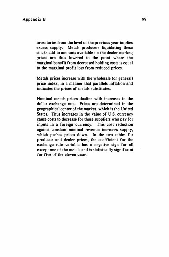
World metals prices are negatively related to metals inventories (or stocks). An increase in metals

Appendix B

inventories from the level of the previous year implies excess supply. Metals producers liquidating these stocks add to amounts available on the dealer market; prices are thus lowered to the point where the marginal benefit from decreased holding costs is equal to the marginal profit loss from reduced prices.

Metals prices increase with the wholesale (or general) price index, in a manner that parallels inflation and indicates the prices of metals substitutes.

Nominal metals prices decline with increases in the dollar exchange rate. Prices are determined in the geographical center of the market, which is the United States. Thus increases in the value of U.S. currency cause costs to decrease for those suppliers who pay for inputs in a foreign currency. This cost reduction against constant nominal revenue increases supply, which pushes prices down. In the two tables for producer and dealer prices, the coefficient for the exchange rate variable has a negative sign for all except one of the metals and is statistically significant for five of the eleven cases.

99

Tab

le B

.1.

Indi

vidu

al M

etal

Equ

atio

ns fo

r P

rodu

cer

Pri

ces

In&

pen

den

t A

lum

inu

m

Cop

per

Lea

d

Afo

!rbd

enum

N

icke

l S

teel

Z

inc

Var

iabl

e

(Dol

lars

per

po

un

d)

Inte

rcep

t 0.

4848

-0

.226

8 -1

.127

9 -0

.514

2 -0

.764

0 -2

.441

6 -1

.100

0 (1

.315

) (-

0.43

3)

(-0.

932)

( -

0.41

4)

(-0.

313)

(-

5.72

8) •

(-

1.63

1)

Wor

ld I

ndus

tria

l -0

.086

8 0.

7636

1.

4821

0.

9848

0.

7422

-0

.568

3 0.

8950

P

rodu

ctio

n ( -

0.36

6)

(3.3

01)

• (1

.937

) (1

.621

) (0

.964

) (-

0.94

8)

(1.5

82)

Met

al S

tock

s -0

.008

8 -0

.482

-0

.109

6 -0

.390

9 -0

.036

3 -.

8256

0.

0141

( -

0.25

2)

(-0.

792)

( -

0.61

2)

(-2.

875)

•

(-0.

287)

(1

.750

) (0

.082

)

Who

lesa

le P

rice

0.

7636

0.

3063

-0

.085

7 0.

9553

0.

7344

0.

9978

0.

4609

In

dex

(8.3

40)

• (2

.384

) •

( -0.

328)

(3

.870

) •

(2.3

16)

• (6

.131

) •

(2.4

25)

•

Exc

hang

e R

ate

-0.2

340

-0.7

191

-0.3

050

-0.8

762

-1.4

334

0.01

70

0.71

49

Inde

x ( -

0.43

0)

(-3.

628)

•

( -0.

358)

(-

5.24

8) •

(-

2.04

9) •

(0

.061

) (1

.203

)

R-S

quar

e 0.

918

0.91

78

0.33

44

0.79

64

0.85

12

0.97

79

0.69

52

F-S

tati

stic

70

.98

70.7

86

4.01

4 24

.468

29

.59

277.

513

15.2

54

(4,2

1)

(4,2

1)

(4,2

0)

(4,2

0)

(4,1

6)

(4,2

1)

(4,2

1)

Dur

bin-

Wat

son

0.88

7 1.

849

1.24

8 1.

848

1.89

5 1.

408

1.22

6 S

tati

stic

SO

UR

CE

: P

rodu

cer

pric

es

for

alum

inum

, co

pper

, le

ad

and

zinc

, S

tand

ard

and

Po

or'

s. C

orpo

rati

on,

Bas

ic

Stat

isti

cs

on

A

feta

ls,

1985

; fo

r m

olyb

denu

m a

nd n

icke

l, A

max

Cor

pora

tion

; for

ste

el, !

BR

D,

Com

mod

ity

Trad

e a

nd

Pri

ce T

rcnd

s(19

86).

• S

tati

stic

ally

sig

nifi

cant

at

.05

leve

l.

Tab

le 8

.2.

Indi

vidu

al M

etal

Equ

atio

ns f

or D

eale

r P

rice

s

Inde

pcnd

t'nf

A

lum

inu

m

Cop

per

Lea

d

Zin

c V

aria

ble

(Dol

lars

per p

ou

nd

)

Inte

rcep

t 2.

1259

-0

.443

4 -2

.243

8 -2

.406

9 (3

.02

6)'

(-

0.48

9)

(-1.

506)

(-

2.21

4) •

Wor

ld I

ndus

tria

l -0

.172

8 1.

4198

1.

9076

2.

3312

P

rodu

ctio

n (-

1.08

2)

(2.8

86)

• (2

.775

) •

(2.6

81)

•

Met

al S

tock

s -0

.117

6 -0

.254

1 -0

.009

8 -0

.205

8 (-

2.13

7) •

(-

2.15

4) •

(-

0.04

5)

(-0.

749)

Who

lesa

le P

rice

0.

8139

-0

.071

6 -0

.315

0 -0

.103

5 In

dex

(10.

982)

•

( -0.

277)

(-

1.27

1)

(-0.

351)

Exc

hang

e R

ate

-3.1

339

-0.4

435

-1.9

137

-0.4

206

Inde

x (-

5.95

5) •

( -

1.17

0)

(-2.

013)

•

( -0.

440)

R-S

quar

c 0.

9614

0.

5646

0.

5409

0.

4954

F-S

tati

stic

14

4.05

9.

106

8.06

9 7.

14

(4,1

9)

(4,2

1 )

(4,2

0)

(4,2

1)

Dur

bin-

Wat

son

2.09

2 1.

691

1.47

8 1.

350

Sta

tist

ic

SO

UR

CE

: D

eale

r pr

ices

, IB

RD

, C

om

mo

m(v

Tra

de a

nd

Pri

ce T

rend

r(19

86).

• S

tati

stic

ally

sig

nifi

cant

at

the

.05

leve

l.

102

§ £ J! ~ c.J

§ £ ~ ~ c.J

Appendix B

Chart B.1. Aluminum - Dealer Price, Basic Equation

lOO~----------------------------------~

80

60

40

20

0 1960

.... ACfUALP.

... PREDICfED P.

1965 1970 I!17S

Year 1980 1985

Price = 2.13 - 0.17 IP - 0.12 Stocks + 0.81 Plndex - 3.13 XRate (3.026) (-1.082) (-2.137) (10.982) (-5.955)

R Square = 0.9614

Chart B.2. Aluminum - Producer Price, Basic Equation

l00~-----------------------------------,

80

60

40

20 1960

.. ACfUALP.

... PREDICfEDP.

1965 1970 I!17S 1980 1985

Year

Price = 0.49 - 0.09 IP - 0.01 Stocks + 0.76 PIndex - 0.23 XRate (1.315) (-0.366) (-0.252) (8.340) (-0.430)

R Square = 0.9180

Appendix B

§ If D

p..

~ U

§ If ~ ~ U

ChartB3. Copper - Dealer Price, Basic Equation

120-.---------------------.

100

80

60

40

20 1960

... ACllJALP.

.... PREDICTEDP.

1965 1970

Year 1975 19110 1985

Price = -0.44 + 1.42 IP - 0.25 Stocks - 0.07 Plndex - 0.44 XRate (-0.489) (2.886) (-2.154) (-0.277) (-1.170)

R Square = 0.5646

Chart B.4. Copper - Producer Price, Basic Equation

120-r--------------------,

100

80

60

40

20 1960

... ACllJALP.

.... PREDICTED P.

1965 1970

Year 1975 19110 1985

Price = -0.23 + 0.76 IP - 0.05 Stocks + 031 PIndex - 0;72 XRate (-0.433) (3.301) (-0.792) (2.384) (-3.628)

R Square = 0.9178

103

104

§ ~

J! tl 5 U

1 ~ ~ ~

~ U

Appendix B

Chart B.s. Lead - Dealer Price, Basic Equation

~~-----------------------------------,

50

40

30

20

10

0 1960

.. ACTIJALP.

... PREDICI"ED P.

1965 1970

Year 1975 1980 1985

Price = - 2.24 + 1.91 IP - 0.01 Stocks - 0.32 Plndex - 1.91 XRate (-1.506) (2.775) (-0.045) (-1.271) (-2.013)

R Square = 0.5409

Chart B.6. Lead - Producer Price, Basic Equation

~~----------------------------------~

50

40

30

20

10

0 1960

- ACTIJALP. ... PREDICI"ED P.

1965 1970 Year

1975 1980 1985

Price = -1.13 + 1.48 IP - 0.11 Stocks - 0.09 PIndex - 0.31 XRate (-0.932) (1.937) (-0.612) (-0.328) (-0.358)

R Square = 0.3344

Appendix B

§ If ~

r:l.

~ U

§ If ~

r:l.

~ U

Chart B.7. Zinc - Dealer Price, Basic Equation

~~--------------------------------,

50

40

30

20

10

0 1960

.... AC1UALP.

... PREDIcrED P.

1965 1970

Year 1975 1980 19&'5

Price = - 2.41 + 2.33 IF - 0.21 Stocks - 0.10 PIndex - 0.42 XRate (-2.214) (2.681) (-0.749) (-0.351) (-0.440)

R Square = 0.4954

Chart B.8. Zinc - Producer Price, Basic Equation

~~--------------------------------~

50.

40

30

20

10 1960

... AC1UALP.

... PREDIcrED P.

1965 1970

Year 1975 1980 19&'5

Price = -1.10+ 0.90 IF + O.OlStocks + 0.46 PIndex + 0.72 XRate (-1.631) (1.582) (0.082) (2.425) (1.103)

R Square = 0.6952

105

106

§ If ~ 5 U

Appendix B

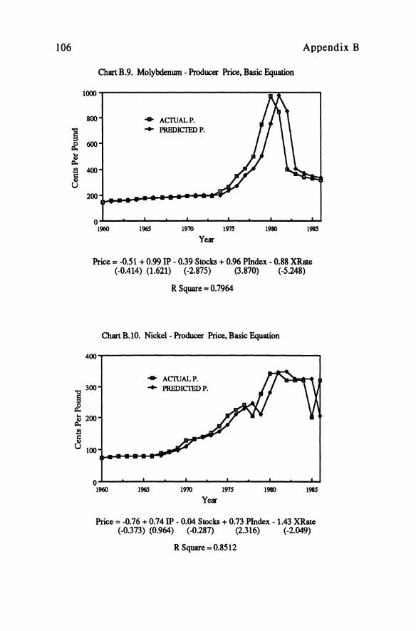
ChartB.9. Molybdenum - Producer Price, Basic Equation

l~~------------------------~~----~

800

600

400

200

0 1960

.. AcruALP.

... PREDICI'ED P.

1965 1970

Year 1m 1980 1985

Price = -0.51 + 0.99 IP - 0.39 Stocks + 0.96 PIndex - 0.88 XRate (-0.414) (1.621) (-2.875) (3.870) (-5.248)

R Square = 0.7964

Chart B.IO. Nickel- Producer Price, Basic Equation

400~--------------------------------~

... AcruALP.

... PREDICI'ED P.

o~--~~--~--~----~--~--~~--~ 1960 1965 1970 1975 1980 1985

Year

Price = -0.76 + 0.74 IP - 0.04 Stocks + 0.73 PIndex - 1.43 XRate (-0.373) (0.964) (-0.287) (2.316) (-2.049)

R Square = 0.8512

Appendix B 107

Chart B.11. Steel - Producer Price, Basic Equation

40~----------------------------------~

... ACIUALP . 30 ... PREDICTED P.

§ ~ ~ ~

20

5 u 10

0 1960 1965 1970 1975 1980 19&5

Year

Price = -2.44 - 0.57 IP+ 0.83 Stocks + 0.99 PIndex + 0.02 XRate (-5.728) (-0.946) (1.750) (6.131) (0.061)

R Square = 0.9779

Appendix C

MARK.ET SUPPLY SHOCK.S

From 1960 through 1986 there were certain disruptions in the individual metals markets that were caused by political decisions, acts of nature or some other factors that have not been explicitly included in our "supply/demand" model. These exogenous supply shocks for the period of the study are identified for the individual metals in Table C.l. In a regression equation, these exogenous supply shocks can be modeled by the inclusion of dummy variables which take on a value of 1 for the year of the shock and zero otherwise. The fifteen dummy variables are added to the pooled price level equation of Table Three. Table C.2 contains the results for the regression model for both producer and dealer metals prices with the inclusion of these dummy variables.

110 Appendix C

Table C.l. Metal Supply Shocks

Aluminum

1963: The U.S. Government institutes a program to dispose of 135,000 short tons of aluminum by mid-1965; 51,589 tons are sold in 1963.

1973: 698,800 short tons of primary aluminum shipped from U.S. Government inventories.

1975: 2,486 tons of primary aluminum shipped from U.S.

Copper

Government inventories. Price increases for primary aluminum ingot delayed until August by the Council on Wage and Price Stability.

1965: 120,000 tons of copper released from U.S. Government inventories.

1976: The transport system used by producers in central Africa is disrupted.

Lead

1964: Production in Africa decreases due to nationalization of some mines.

1972: U.S. Government price controls go into effect until December of 1973.

1973: U.S. Government stockpile objective for lead is reduced, as 211,541 tons is withdrawn from producer and government stocks. The U.S. lead price advanced to a record high in 1974 following the removal of price controls in December 1973.

Appendix C 111

Table C.l. Metal Supply Shocks (continued)

Lead (continued)

1982: Revised Environmental Protection Agency (EPA) regulations concerning the use of lead in gasoline become effective. The new standard is 1.10 grams per gallon absolute limit for all leaded gasoline, including imports, with no exceptions for small refiners after July 1, 1983.

Molybdenum

1973: 36.5 million pounds of molybdenum from u.S. Government stockpile authorized for disposal.

1974: 35 million pounds of molybdenum shipped from u.S. Government stockpile.

Nickel

1970: Canadian labor strike reduces supply; most of the industry is affected in the early part of the year.

1980: The "Superfund Act" authorizes a $0.225 tax per pound of pure nickel produced in or brought into the United States.

Zinc

1976: Increase in the U.S. Government stockpile goal for zinc from 374,830 tons to 1,313,000 tons eliminates any excess for disposal.

1980: U.S. Government stockpile goal is reduced from 1,313,000 tons to 1,292,739 tons.

Tab

le C

.2.

Pri

ce L

evel

Equ

atio

ns w

ith

Sup

ply

Sho

cks

Inde

pend

cot

D,'a

ler P

rice

s P

rodu

cer P

rice

s V

aria

ble

(Dol

lars

per

po

un

d)

Inte

rcep

t -0

.555

6 0.

2832

(-

5.59

8) *

(1

.315

)

Wor

ld I

ndus

tria

l 2.

2765

0.

4034

P

rodu

ctio

n (6

.062

) •

(2.1

74)

* M

ctal

Sto

cks

-0.1

603

-0.0

684

(-2.

623)

•

(-1.

620)

Who

lesa

le P

rice

0.

2316

0.

4751

In

dex

(1.2

48)

(5.8

23)

* E

xcha

nge

Rat

e 0.

4480

-0

.364

0 In

dex

(2.8

69)

* (-

4.05

1) *

D

I V

aria

ble

-1.2

054

-0.2

960

Alu

min

um

(-2.

115)

•

(-2.

801)

•

D2

Var

iabl

e -3

.768

8 -1

.096

0 L

ead

(-8.

035)

•

(-10

.569

) •

D3

Var

iabl

e -1

.966

8 -0

.800

8 Z

inc

(-7.

441)

' (-

9.15

2) •

D4

Var

iabl

e N

/A

-1.5

774

Ste

el

(-16

.921

) •

D5

Var

iabl

e N

/A

1.09

95

Nic

kel

(9.9

25)

•

D6

Var

iabl

e N

/A

1.62

87

Mol

ybde

num

(1

5.76

0) •

D7

19

63

-0

.020

8 -0

.075

3 A

lum

inum

(-

0.09

0)

(-0.

499)

D9

19

73

0.

1740

-0

.264

3 A

lum

inum

(0

.751

) (-

1.74

2)

DIO

197

5 -0

.068

1 0.

0788

A

lum

inum

(-

0.29

1)

(0.5

23)

Tab

leC

.2.

Pri

ce L

evel

Equ

atio

ns w

ith

Supp

ly S

hock

s (c

ontin

ued)

01

11

96

4

0.66

84

0.20

81

Lea

d (2

.884

) •

(1.3

55)

D24

1972

0.

2274

0.

0259

L

ead

(1.9

94)

(0.1

71)

D12

1973

0.

4076

-0

.072

3 L

ead

(1.7

88)

(-0.

478)

D2.

.'i 19

82

-0.0

444

-0.2

659

Lea

d (-

0.19

2)

(-1.

757)

01

51

97

6

-0.0

643

0.06

41

Zin

c (-

0.28

2)

(0.4

25)

D17

1980

0.

0192

-0

.064

9 Z

inc

(0.0

84)

(-0.

432)

D18

1965

0.

1481

-0

.012

8 C

oppe

r (0

.650

) (-

0.08

5)

D19

1976

0.

0046

0.

0686

C

oppe

r (0

.020

) (0

.447

)

D20

1970

N

/A

0.07

86

Nic

kel

(0.5

15)

D26

1980

N

/A

0.20

54

Nic

kel

(1.3

56)

D22

1973

N

/A

0.19

19

Mol

ybde

num

(-

1.26

6)

D23

1974

N

/A

-0.0

518

Mol

vbde

num

__

(-0.

34])

R-S

quar

e 0.

6190

0.

9295

F-S

tati

stic

16

.973

94

.342

(1

8,15

9)

(2..'1

,152

)

Durbin-Wat~~__

\,261

1.

S41

SO

UR

CE

S:

Dea

ler

pric

es,

ilkt

als

W

eei-

(var

ious

is

sues

), IB

RD

, C

omm

odJ(

y T

rade

a

od

Pri

ce

Tr,'o

ds

(198

6);

Pro

duce

r pr

ices

fo

r al

umin

um,

copp

er,

lead

an

d

zinc

, S

tand

ard

and

Poo

r's

Cor

pora

tion

, B

asic

St

atis

tics

00

il

k/al

s,

1984

, an

d U

.S.

Bur

eau

of

Min

es,

ilfiD

L'ra

l C

omm

otfi(

Y St

lmm

arks

1~ f

or m

olyb

denu

m a

nd n

icke

l, A

max

Cor

pora

tion

.

• st

atis

tica

lly

sign

ific

ant

Appendix D

CALCULATION OF THE MARK.ET MODEL RESIDUALS

Residuals from the market model can be used to evaluate firm-specific performance, both over a period of time and cross­sectionally, of a stock price relative to the market. An individual company price would change with respect to that company's competitive position, while the market relative price would not.

Description

The relative value in the stock market of individual firms is determined by using the market model. In the market model the individual firm returns are regressed on the equally weighted market index of returns compiled by the Center for Research in Security Prices (University of Chicago).1 Returns are defined as the change in price plus dividends in a year. Thus the relationship between the market returns and individual firm returns can be expressed as:

R· t = A + B·R t + e· t 11m 1

1For a detailed discussion of the market model and its underlying assumptions refer to Chapter 3 of Foundations of Finance by E\lgene Fama. A detailed analysis of the event study methodology and the calculation of the market model residuals and the cumulative residuals is done in "Adjustment of Shock Prices to New Information" by Fama, Fisher, Jensen and Roll (1969).

116

where

Appendix D

Rit = Returns for firm i in period t Rmt = Return for the equally weighted market index A = Market model intercept Bi = Systematic risk of security i eit = Market model residual.

It is assumed that eit has a normal distribution with a mean zero and a variance s2(eit).

Here the market model is interpreted as consisting of more than just a statistical relation. The return on the equally weighted market portfolio (Rmt) is assumed to reflect the effects of all the variables on the returns of most of the securities. The residual eit is presumed to capture the effects of the variables that are 1 um-specific. Thus in the market model, securities returns are caused by market factors biRmt' and the remaining firm-specific factors e·t" The residuals eit provide for the analyst a measure not orthe effects of the marketwide factors on returns, but of the effects of company-specific conditions.

Results

Table Twenty-Two compares the performance for three firms and the metals industry as a whole from 1975 through 1986. Alcan is the largest aluminum-producing firm in North America, INCO is the largest nickel-producing firm in the world, and Amax is the world's largest molybdenum producer. The "metals industry" consists of an equally weighted portfolio of all the firms on the New York Stock Exchange and the American Stock Exchange that are listed as metals producers (the firms that have the Standard Industrial Classification Code of 3310 or 3370 are included). The equally weighted portfolio of the metals industry thus constructed has a total of 28,265 monthly stock returns.

The monthly returns for the four individual firms and the portfolio of the metals-producing firms, from January 1965 to December 1974, are regressed on the equally weighted market index for the same period. The estimated values of the alpha and beta coefficients for the individual firms and the metals industry are shown in Table D.1. The beta value for the three firms is less than 1.0, indicating that they are less risky than the total market. The beta coefficient for the metals industry is greater than 1.0, which implies a higher than total market risk for the industry

Appendix D 117

(the inclusion of smaller firms may have caused the portfolio's risk factor to increase).1

The estimated alpha and beta coefficient values are used to calculate the monthly market model residuals from January 1975 to December 1986 for the individual companies and the portfolio of metals firms. The log value of 1.0 plus the monthly abnormal return is then added for each 36-month period in Table Twenty­Two. The exponential of this summed value for the 36-month period gives the cumulative value of the firm's abnormal return. The cumulative residuals are a measure of firm-specific performance as shown in Table 0.2. They suggest that the larger firms were generally performing better than the overall metals industry during the estimation period.

An important assumption underlying the results is that the values of the alpha and beta coefficients are constant. In order to test this assumption, we estimated the market model coefficients for five-year periods from 1965 through 1984. The coefficient values from the different five-year market models from 1965 through 1984 were found to be reasonably stationary across the study period.

1 For a discussion of the comparative risk of market model coefficients for small and large firms, refer to Chapter 4 of Foundations of Finance by Eugene Fama.

Tab

le 0

.1.

Mar

ket M

odel

for

Ind

ivid

ual M

etal

Fir

ms

and

the

Indu

stry

Inde

pend

ent

Aka

n

Am

aK

INC

O

Met

al I

ndus

fly

Var

iabl

e

(Sho

wn

in p

erce

ntag

e)

Inte

rcep

t 0.

001

0.00

5 0.

000

0.00

4

Mar

ket R

etur

n 0.

838

0.76

1 0.

941

1.14

32

Peri

od

1%5-

74

1965

-74

1965

-74

1965

-74

Num

ber

of O

bser

vati

ons

120

120

120

120

Tab

leD

.2.

Cum

ulat

ive

Mar

ket M

odel

Res

idua

ls fo

r M

etal

Pro

duci

ng F

irm

s

Per

iod

A/c

an

A

/coa

A

sarc

o A

mll

K

Phe

lps

INC

O

US

Ste

e/

Met

al

Do

dg

e In

dust

ries

{Cit

=

Hit

-(A

i +

BiH

md

l

(Sho

wn

in pe

rcen

tage

)

1975

1.

08%

33

.70%

2.

71%

59

.63%

32

.17%

25

.17%

79

.46%

-7

.92%

1976

23

.77

52.1

6 33

.24

30.6

6 20

.07

35.5

5 19

.75

4.33

1977

16

.10

-15.

71

-6.7

3 -3

6.84

-4

4.48

-4

4.82

-3

2.78

-6

.06

1978

36

.29

6.99

-5

.02

41.0

5 0.

42

-3.7

9 -2

8.34

-2

.40

1979

46

.47

20.7

4 18

3.86

47

.01

53.9

2 54

.62

-11.

26

7.46

1980

48

.12

14.2

6 20

.74

-5.0

0 27

.23

-11.

63

52.8

4 -1

2.76

1981

-2

6.02

-8

.53

-38.

08

20.3

5 -6

.65

-27.

83

29.2

3 5.

76

1982

29

.61

28.9

8 15

.58

-52.

48

-15.

37

-15.

95

-23.

68

-28.

63

1983

46

.28

49.2

7 4.

17

10.0

5 -1

0.22

26

.24

50.4

3 9.

52

1984

-2

4.65

-1

4.75

-3

5.95

-3

0.94

-4

5.04

-1

3.89

-1

0.68

-2

1.25

1985

5.

19

7.79

-3

.29

-15.

67

65.7

7 8.

70

5.97

-2

0.39

1986

-0

.03

-9.1

9 -1

9.05

-1

1.01

-9

.78

-9.9

7 -1

4.59

-2

1.75

SO

UR

CE

: D

ata

obta

ined

from

Cen

ter

for

Res

earc

h in

Sec

urit

y Pr

ices

(U

nive

rsity

of

Chi

cago

).

NO

TE

S:

Th

e cu

mul

ativ

e m

arke

t m

odel

re

sidu

als

are

calc

ulat

ed

by

usin

g th

e m

arke

t m

odel

fo

r ea

ch

firm

. S

ee

App

endi

x D

fo

r m

etho

dolo

gy.

The

cu

mul

ativ

e re

turn

s ar

e co

ntin

uous

ly

com

poun

ded

for

the

twel

ve

12-m

onth

pe

riod

s by

ad

ding

th

e na

tura

l lo

g o

f (1

+

eit

)

and

then

ta

king

th

e ex

pone

ntia

l of

th

e su

mm

ed

valu

e,

this

pr

oces

s gi

ves

one

plus

th

e ab

norm

al

retu

rns

for

the

peri

od.

The

n on

e is

su

btra

cted

fr

om

the

valu

e to

arr

ive

at t

he c

ontin

uous

ly c

ompo

unde

d ab

norm

al r

etur

ns.

Appendix E

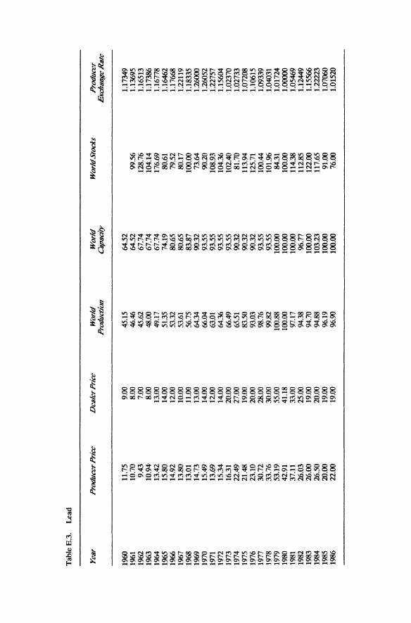
DATA SERIES

Tables E.l through E.8 contain the data used to calculate the various price level and dynamic equations. In each of the tables, the sources of the data set are given. The following is a list of the sources used:

American Bureau of Metals Statistics, Inc. Non-Ferrous Metals Data. New York: American Bureau of Metal Statistics, various issues.

International Bank for Reconstruction and Development. Commodity Trade and Price Trends. Washington, D.C.: IBRD, 1984 and 1986.

Metallgesellschaft A.G. Metal Statistics. Frankfurt am Main: MAG:, various years.

Standard and Poor's Corporation. Basic Statistics on Metals. New York: S&P, 1984.

United Nations. Monthly Bulletin of Statistics. New York: U.N., various issues.

United States Bureau of Mines. Minerals Yearbook. Washington, D.C.: Department of the Interior, various years.

United States Bureau of Mines. Mineral Commodity Summaries. Washington, D.C.,: Department of the Interior, 1984,1985, 1987 and 1988.

Dimensions of all data are as follows: Prices are in dollars per pound; production, capacity, world stocks and exchange rates are indexed to the year 1980; and, also industrial production (GNP) and the wholesale price index are indexed to the year 1980.

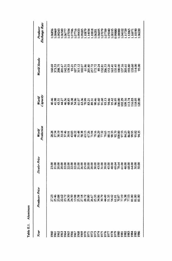
Tab

le E

.1.

Alu

min

um

Yea

r P

rodu

cer P

rice

D

eale

r Pri

ce

Wor

ld

Wor

ld

Wor

ld S

tocK

s P

rodu

cer

Pro

duct

ion

Cap

aci(

v E

xcha

nge

Ra

te

1960

27

.23

23.0

0 28

.28

40.4

6 16

0.69

1.

0685

6 19

61

25.4

6 21

.00

27.5

4 41

.98

373.

53

1.08

469

1962

23

.88

20.0

0 30

.19

43.5

1 29

8.75

1.

0924

3 19

63

22.6

2 20

.00

33.1

8 44

.27

201.

67

UJ6

500

1964

23

.72

22.0

0 37

.46

46.5

6 14

2.51

1.

0677

7 19

65

24.5

0 22

.00

39.9

1 48

.85

139.

33

1.07

034

1966

24

.50

22.0

0 43

.83

50.3

8 93

.21

1.07

596

1967

13

.98

22.0

0 48

.22

54.9

6 10

7.73

1.

0771

6 19

68

25.5

8 21

.00

51.4

8 61

.07

315.

12

1.09

433

1969

27

.18

26.0

0 58

.38

63.3

6 10

2.07

1.

0928

5 19

70

28.7

2 25

.00

63

.B

70.9

9 61

.86

1.10

879

1971

29

.00

20.0

0 67

.26

83.2

1 20

1.80

1.

1493

4 19

72

26.6

7 20

.00

71.9

4 89

.31

257.

72

1.10

818

1973

25

.33

30.0

0 79

.16

90.4

6 17

2.72

1.

0620

1 19

74

34.0

6 43

.00

86.2

9 91

.60

89.2

4 1.

0669

5 19

75

39.7

9 31

.00

77.3

2 91

.60

132.

81

1.07

079

1976

44

.49

39.0

0 79

.65

93.1

3 20

6.53

1.

0770

9 19

77

51.3

5 45

.00

88.1

1 94

.66

153.

20

1.05

040

1978

54

.42

48.0

0 90

.33

95.4

2 16

5.41

1.

0019

5 19

79

61.0

1 69

.64

92.7

0 96

.95

135.

45

0.99

880

1980

70

.87

78.6

4 10

0.00

10

0.00

10

0.00

1.

0000

0 19

81

77.1

9 61

.00

97.5

3 10

2.29

13

7.16

1.

0410

2 19

82

76.3

8 48

.00

84.2

5 10

9.16

20

5.61

1.

1172

9 19

83

77.5

3 68

.00

86.8

9 11

3.74

19

3.80

1.

1296

5 19

84

81.0

0 64

.00

99.9

5 11

6.03

13

3.60

1.

1697

1 19

85

81.0

0 50

.00

95.8

2 11

8.05

11

4.00

1.

1019

0 19

86

81.0

0 50

.00

94.3

5 12

0.00

95

.00

1.06

220

Tab

leE

.2.

Co

pp

er

Yea

r P

rodu

cer P

rice

D

eale

r Pri

ce

Wor

ld

Wor

ld

Wor

ld St

ocK

s P

rodu

cer

Pro

duct

ion

Cap

aci(

v E

Kcn

ange

Ra

te

1960

32

.16

31.0

0 58

.88

56.8

4 36

.36

1.14

871

1961

30

.15

29.0

0 60

.63

59.3

2 53

.09

1.14

647

1962

30

.83

29.0

0 62

.11

60.5

4 51

.16

1.09

622

1963

30

.83

29.0

0 63

.14

61.2

6 59

.11

1.15

473

1964

32

.18

44.0

0 67

.83

63.0

8 58

.46

1.16

017

1965

35

.02

59.0

0 71

.13

68.0

6 40

.07

1.15

281

1966

35

.83

70.0

0 72

.98

71.0

9 48

.22

0.94

719

1967

37

.92

52.0

0 67

.26

73.7

0 44

.54

0.94

102

1968

41

.17

56.0

0 76

.03

83.5

3 40

.65

1.19

692

1969

47

.43

67.0

0 82

.52

89.8

3 46

.25

0.95

822

1970

58

.07

64.0

0 86

.74

91.7

7 47

.27

0.96

168

1971

52

.09

49.0

0 82

.05

99.3

6 59

.47

0.94

910

1972

51

.28

49.0

0 89

.78

99.7

8 58

.92

0.92

728

1973

59

.30

81.0

0 93

.90

104.

57

70.4

5 0.

9108

2 19

74

77.0

6 94

.00

96.6

9 10

5.24

49

.37

0.90

592

1975

64

.72

56.0

0 88

.11

105.

54

97.5

6 0.

9030

9 19

76

69.4

6 64

.00

93.4

4 10

5.97

18

5.60

0.

9335

8 19

77

66.4

9 60

.00

96.7

3 10

6.03

19

7.38

0.

9628

6 19

78

72.3

8 62

.00

98.1

7 10

6.48

20

7.51

0.

9548

4 19

79

91.8

0 90

.00

99.9

3 10

5.51

16

2.58

0.

9867

5 19

80

102.

20

99.0

0 10

0.00

10

0.00

10

0.00

1.

0000

0 19

81

85.5

9 79

.00

103.

53

100.

90

90.4

9 1.

0084

8 19

82

74.5

6 67

.00

100.

58

102.

04

95.6

9 1.

1546

1 19

83

78.1

8 72

.00

103.

26

102.

69

147.

84

1.27

954

1984

72

.07

63.0

0 10

1.75

11

0.59

13

8.99

1.

4891

2 19

85

69.0

0 63

.00

103.

11

97.6

7 10

0.00

1.

6877

0 19

86

68.0

0 63

.00

105.

24

98.2

9 88

.00

1.80

820

Tab

leE

.3.

Lea

d

Yea

r P

rodu

cer P

rice

D

eale

r Pri

ce

Wor

ld

Wor

ld

Wor

ld St

ocK

s P

rodu

cer

Pro

duct

ion

Cap

acit

y E

Kch

ange

Ra

te

1960

11

.75

9.00

45

.15

64.5

2 1.

1734

9 1%

1 10

.70

8.00

46

.46

64.5

2 99

.56

1.13

695

1962

9.

43

7.00

45

.62

67.7

4 12

8.76

1.

1651

3 19

63

10.9

4·

8.00

48

.00

67.7

4 10

4.14

1.

1738

6 19

64

13.4

2 13

.00

49.1

7 67

.74

176.

69

1.16

778

1%5

15.8

0 14

.00

51.3

5 74

.19

80.6

1 1.

1646

2 19

66

14.9

2 12

.00

53.3

2 80

.65

79.5

2 1.

1766

8 19

67

13.8

0 10

.00

53.6

1 80

.65

80.1

7 1.

2211

9 19

68

13.0

1 11

.00

56.7

5 83

.87

100.

00

1.18

335

1969

14

.73

13.0

0 64

.34

90.3

2 73

.64

1.26

000

1970

15

.49

14.0

0 66

.04

93.5

5 90

.20

1.26

052

1971

13

.69

12.0

0 63

.01

93.5

5 10

8.93

1.

2275

7 19

72

15.3

4 14

.00

64.3

6 93

.55

104.

36

1.15

604

1973

16

.31

20.0

0 66

.49

93.5

5 10

2.40

1.

0237

0 19

74

22.4

9 27

.00

65.5

1 90

.32

81.7

0 1.

0273

3 19

75

21.4

8 19

.00

83.5

0 90

.32

113.

94

1.07

208

1976

2.

UO

20

.00

93.0

3 90

.32

125.

71

1.10

615

1977

30

.72

28.0

0 98

.76

93.5

5 10

0.44

1.

0933

9 19

78

33.7

6 30

.00

99.8

2 93

.55

101.

%

1.04

031

1979

53

.19

55.0

0 10

0.88

10

0.00

84

.31

1.01

724

1980

42

.91

41.1

8 10

0.00

10

0.00

10

0.00

1.

0000

0 19

81

37.1

1 33

.00

97.1

7 10

0.00

11

4.38

1.

0546

9 19

82

26.0

3 25

.00

94.3

8 96

.77

112.

85

1.12

449

1983

26

.00

19.0

0 94

.70

100.

00

122.

00

1.15

566

1984

26

.50

20.0

0 94

.88

103.

23

117.

65

1.22

223

1985

20

.00

19.0

0 %

.19

100.

00

91.0

0 1.

0706

0 19

86

22.0

0 19

.00

%.9

0 10

0.00

76

.00

1.01

520

Tab

leE

.4.

Nic

kel

Ye

ar

Pro

duce

r Pri

ce

Wor

ld P

rodu

ctio

n W

orld

Cap

acit

y W

orl

d St

ocK

s P

rodu

cer

Exc

hang

e .R

ate

1960

74

.00

45.9

2 41

.56

0.89

019

1961

78

.00

49.6

6 42

.26

0.91

978

1962

80

.00

45.%

42

.45

0.94

236

1963

79

.00

46.7

7 42

.64

0.95

981

1964

79

.00

50.2

7 44

.73

0.96

620

1965

79

.00

57.5

9 47

.91

88.1

4 0.

9550

6 19

66

79.0

0 54

.75

50.5

1 71

.75

0.96

302

1967

88

.00

58.0

5 52

.22

159.

89

0.96

246

1968

94

.00

66.2

5 54

.89

158.

76

0.97

197

1969

10

5.00

62

.42

60.8

5 14

0.68

1.

0160

8 19

70

129.

00

86.9

2 71

.64

84.7

5 1.

0059

4 19

71

133.

00

84.9

9 79

.95

126.

55

0.96

233

1972

14

0.00

85

.56

SO.5

2 84

.49

0.91

608

1973

15

3.00

97

.76

81.8

5 13

4.46

0.

8991

1 19

74

174.

00

109.

98

88.5

2 14

7.46

0.

9151

4 19

75

207.

00

111.

10

94.2

9 23

2.20

0.

9082

9 19

76

225.

00

111.

30

%.3

8 18

1.36

0.

9129

1 ]9

77

241.

00

113.

10

97.2

1 16

2.15

0.

9730

1 19

78

205.

00

83.2

2 97

.97

95.4

8 0.

9734

0 19

79

275.

00

87.4

6 99

.62

104.

52

1.00

384

1980

34

1.00

10

0.00

10

0.00

10

0.00

1.

0000

0 19

81

343.

00

90.3

6 99

.56

71.1

9 1.

0735

8 19

82

320.

00

80.1

6 10

4.44

11

8.08

1.

1966

5 19

83

320.

00

83.8

1 10

5.90

96

.61

1.29

383

1984

32

0.00

92

.69

104.

19

107.

34

l.32

683

1985

20

1.00

98

.17

101.

27

117.

36

1.33

660

1986

32

0.00

87

.64

98.9

7 10

3.31

1.

3621

0

Tab

le E

.5.

Mol

ybde

num

Yea

r P

rodu

cer P

rice

W

orld

Pro

duct

ion

Wo

rld

Cap

aciQ

-' W

orl

d St

ocK

s P

rodu

cer

Exc

lJao

ge K

ate

1960

14

7.00

35

.01

28.3

6 0.

9532

7 19

61

155.

00

34.6

3 28

.36

45.8

3 0.

9529

0 19

62

160.

00

27.4

5 21

.45

43.0

8 0.

9219

5 19

63

160.

00

35.1

5 27

.27

29.1

7 0.

9043

1 19

64

171.

00

36.4

6 28

.36

34.7

2 0.

8839

0 19

65

175.

00

46.1

1 28

.36

33.3

3 0.

8979

5 19

66

175.

00

58.5

0 36

.00

40.2

8 0.

8902

0 19

67

181.

00

59.1

7 43

.64

70.8

3 0.

8833

3 19

68

182.

00

59.9

4 46

.55

95.8

3 0.

9096

9 19

69

189.

00

66.7

6 52

.00

98.6

1 0.

9123

7 19

70

192.

00

75.4

1 61

.82

102.

78

0.89

361

1971

19

2.00

70

.18

61.8

2 13

8.89

0.

8775

5 19

72

192.

00

73.4

9 61

.82

168.

06

0.88

018

1973

19

2.00

75

.88

61.8

2 17

3.61

0.

8844

4 19

74

230.

00

77.7

7 61

.82

151.

39

0.83

598

1975

26

2.00

73

.35

65.4

5 13

6.11

0.

8569

1 19

76

345.

00

81.8

4 69

.09

130.

56

0.87

313

1977

40

1.00

88

.14

72.7

3 12

2.22

0.

9200

2 19

78

495.

00

90.9

9 80

.00

119.

44

0.96

355

1979

75

0.00

94

.75

80.0

0 11

2.50

0.

9902

3 19

80

970.

00

100.

00

100.

00

100.

00

1.00

000

1981

85

0.00

98

.19

109.

09

151.

36

1.01

621

1982

40

0.00

89

.11

120.

00

205.

56

1.21

219

1983

36

5.00

49

.19

120.

00

251.

39

1.98

807

1984

34

0.00

82

.96

120.

00

201.

39

2.06

897

1985

33

0.00

85

.75

120.

00

150.

00

4.74

900

1986

31

4.00

75

.82

94.2

3 65

.00

4.52

720

Tab

leE

.6.

Ste

el

Yea

r P

rodu

cer P

rice

W

orl

d SI

OC

KS

Pro

t/uc

er

Exc

ha

ng

e R

ate

1960

6.

00

51.8

2 1.

2570

5 19

61

5.00

53

.30

1.25

754

1962

5.

00

53.4

2 1.

2541

8 19

63

6.00

57

.77

1.23

764

1964

6.

00

66.9

8 1.

2454

5 19

65

6.00

69

.69

1.24

116

1966

6.

00

71.2

8 1.

2485

4 19

67

6.00

74

.46

1.28

016

1968

6.

00

79.9

9 1.

3002

7 19

69

7.00

88

.12

1.30

342

1970

7.

00

90.3

1 1.

2906

5 19

71

fWO

85

.15

1.26

400

1972

fW

O

93.4

0 1.

1848

6 19

73

9.00

10

5.57

1.

1163

7 19

74

12.0

0 10

6.34

1.

1913

3 19

75

13.0

0 91

.06

1.13

840

1976

13

.00

97.4

1 1.

1473

4 19

77

15.0

0 94

.74

1.09

084

1978

17

.00

100.

00

0.98

513

1979

18

.00

106.

37

0.98

711

1980

21

.00

100.

00

1.00

000

1981

23

.00

99.0

4 1.

0358

9 19

82

24.0

0 85

.63

1.11

872

1983

26

.00

87.4

1 1.

1124

4 19

84

27.0

0 89

.00

1.15

649

1985

28

.00

86.0

0 1.

0078

0 19

86

25.0

0 84

.00

0.86

990

Tab

le E

.7.

Zin

c

Yea

r P

rodu

cer P

rice

D

eale

r Pri

ce

Wor

ld

Wor

ld

Wor

ld S

tocl

s P

rodu

cer

Pro

due/

ion

Cap

acit

y &

c/Ja

nge

Ra

tc

1960

12

.96

11.0

0 53

.84

51.7

2 52

.67

1.30

283

1%

1

11.5

5 10

.00

57.3

5 53

.45

53.4

2 1.

2968

3 19

62

11.6

3 8.

00

59.1

5 59

.90

53.8

5 1.

2825

6 19

63

12.0

1 10

.00

61.0

7 59

.90

57.4

5 1.

1706

5 19

64

13.5

7 15

.00

66.0

2 60

.34

57.3

3 1.

1842

6 19

65

14.5

0 14

.00

69.6

7 65

.52

47.1

2 1.

1791

5 19

66

14.5

0 13

.00

73.3

1 68

.97

46.8

8 1.

1936

0 19

67

13.8

5 12

.00

72.7

8 74

.14

52.0

4 1.

2053

3 19

68

13.5

0 12

.00

80.9

8 74

.14

55.4

1 1.

2272

4 19

69

14.6

5 13

.00

88.1

0 77

.59

57.5

7 1.

2366

6 19

70

15.3

2 13

.00

89.1

1 77

.59

54.3

3 1.

2595

9 19

71

]6.1

4 14

.00

84.2

1 81

.03

62.3

8 1.

2397

3 19

72

17.7

2 17

.00

93.0

5 84

.48

81.9

7 1.

1727

5 19

73

20.2

6 39

.00

95.5

1 87

.93

73.8

0 1.

0805

8 19

74

35.9

4 56

.00

94.8

5 87

.93

70.3

1 1.

1762

0 19

75

38.9

0 34

.00

83.3

8 89

.66

55.0

5 1.

1569

7 19

76

37.4

5 32

.00

91.6

7 91

.38

91.2

3 1.

1129

5 19

77

34.3

8 27

.00

94.7

3 96

.55

137.

74

1.11

278

1978

31

.14

27.0

0 95

.33

98.2

8 13

7.14

0.

9838

8 19

79

38.8

6 34

.00

104.

66

98.2

8 14

3.63

0.

9934

0 19

80

38.0

3 35

.00

100.

00

100.

00

100.

00

1.00

000

1981

45

.42

38.0

0 10

1.67

10

0.00

10

4.45

1.

0356

6 19

82

40.2

4 34

.00

96.7

4 10

1.72

94

.59

1.11

468

1983

43

.02

35.0

0 10

3.91

10

5.17

10

5.17

1.

1273

8 19

84

50.0

0 42

.00

108.

71

108.

62

96.2

7 1.

1666

7 19

85

42.0

0 33

.00

111.

46

113.

61

77.0

0 1.

1539

0 19

86

41.0

0 35

.00

108.

86

117.

48

78.0

0 1.

0084

0

Tab

le E

.g.

Oth

er D

ata

Yea

r

1960

1%

1 1%

2 1%

3 19

64

1965

19

66

1967

1%

8 19

69

1970

19

71

1972

19

73

1974

19

75

1976

19

77

1978

19

79

1980

19

81

1982

19

83

1984

19

85

1986

Indu

stri

al G

NP

40.7

42

.6

45.4

48

.0

51.8

55

.2

59.0

60

.5

64.5

70

.5

71.2

74

.2

79.3

86

.2

87.2

81

.4

88.5

92

.1

95.7

10

0.4

100.

0 10

0.1

97.6

10

0.6

104.

9 10

6.3

108.

1

Who

lesa

le P

rire

Ind

ex

26

26

27

27

28

29

30

31

32

33

34

36

38

43

52

57

63

69

74

85

100

113

125

139

160

171

182

INDEX

Adelman, MA. 20 A1can 75 Aluminum 33, 39, 56, 59, 61, 75

capacity 39, 75, 80 inventories 6 prices 2,23,39,41,67,71,74,78

Amax 54, 75, 78

Baily, Martin N. 28 Ball, Raymond 8,9,20 Bohi, Douglas 28 Bosworth, Barry 7, 19 Brimelow, Peter 54 By-products 20

Capacity 18, 55 CODELCO 62 Competitive conditions 53, 54, 61, 69, 70,

73,74,87 Cooper, Richard N. 9 Cootner, Paul H. 28 Copper 8,33,39,41,55

capacity 6 prices 2, 10,23,41

Dealer prices 12-14,23,26,28,30,38,46, 67,69,71

definition 13

Equation-estimated prices 30, 46, 71, 87 Exchange rates (as a determining variable)

18, 19, 26, 28, 29, 34, 36, 38, 78

Fisher, Franklin M. 28 Forecast prices 82, 84, 87

base 1990 case 84,87 expanded capacity 84 expanded supply 87

Funkhauser, Richard 20

General price index (as a determining variable) 17, 19,26

inflation 28, 82, 84

Harnett, Donald L. 28 Herfindahl Index 56,59,73 Hubbard, Glenn R 28

INCO 54, 75, 78 Industrial production 17,19,25,26,28,30,

82

Lawrence, Robert Z. 7,9, 19 Lead 33,55

prices 2,10,30,41 Lerner Index 69, 74

MacAvoy, Paul Vf. 20,55,56 MacKinnon, James G. 28 MacGregor, Ian v Market deconcentration 55, 56 Market equilibrating argument 2, 4, 7, 28,

29,44,46,50 competition 87 demand 5,16,17,33,87 supply 5,6, 17, 18, 87

Marks, Robert 8,9,20 McNicol, David L. 12 Molybdenum 33, 39, 56, 59, 61, 62, 75

capacity 25, 75 inventories 2 prices 1, 10, 24, 44, 67, 71, 74, 78

Nickel 13, 33, 39, 54, 56, 59, 61, 75 capacity 61, 75 prices 2,24,25,44,67,71,78

Olewiler, Nancy D. 28 Orr, David 55

Pindyck, Robert S. 26, 28 Pooling prices 25 Price change equation 10, 21, 22, 45, 46, 84 Price determinants 14 Price level equation 10, 19, 25, 26, 28, 29,

34,46,71,74,82,84,87 entrants share 41 post-l980 demand reductions 34 ·status quo· 38

Producer prices 12-14,23,28,30,46,71 definition 13

Rubinfeld, Daniel L. 26, 28

Scrap 59,73 Security price reaction 78 Speculative-political disequilibrating argument 4, 7-9, 20, 51

government objectives 4, 5, 8, 9, 20, 21, 45,87

speculation 4, 7, 9, 20, 21, 45 Steel 18, 39, 41, 56

inventories 6 pri~es 2, 10

Stocks (as a determining variable) 17-19, 25,26,28,36,38,44,78

Index

Stundza, Tom 4, 5 Substitutions 5 Supply expansion 6, 39, 41, 53, 61, 70, 74,

75,2,87 Supply restriction 71, 73, 75 Supply shocks 38 Swing producer 54, 71, 74, 75, 80

Technology 2, 30

Verleger, Philip K. 28

Walde, Thomas 9

Zinc 39,55 prices 2, 10, 41, 82

132