Reference Manual for the System Advisor Model’s Wind Power ... · Reference Manual for the System Advisor Model’s Wind ... Wind farm hourly electrical output ... Turbine power

NREL is a national laboratory of the U.S. Department of Energy Office of Energy Efficiency & Renewable Energy Operated by the Alliance for Sustainable Energy, LLC This report is available at no cost from the National Renewable Energy Laboratory (NREL) at www.nrel.gov/publications.

Contract No. DE-AC36-08GO28308

Reference Manual for the System Advisor Model’s Wind Power Performance Model Janine Freeman and Jennie Jorgenson National Renewable Energy Laboratory

Paul Gilman and Tom Ferguson Independent Consultants

Technical Report NREL/TP-6A20-60570 August 2014

NREL is a national laboratory of the U.S. Department of Energy Office of Energy Efficiency & Renewable Energy Operated by the Alliance for Sustainable Energy, LLC This report is available at no cost from the National Renewable Energy Laboratory (NREL) at www.nrel.gov/publications.

Contract No. DE-AC36-08GO28308

National Renewable Energy Laboratory 15013 Denver West Parkway Golden, CO 80401 303-275-3000 • www.nrel.gov

Reference Manual for the System Advisor Model’s Wind Power Performance Model Janine Freeman and Jennie Jorgenson National Renewable Energy Laboratory

Paul Gilman and Tom Ferguson Independent Consultants

Prepared under Task No. WE11.1214

Technical Report NREL/TP-6A20-60570 August 2014

NOTICE

This report was prepared as an account of work sponsored by an agency of the United States government. Neither the United States government nor any agency thereof, nor any of their employees, makes any warranty, express or implied, or assumes any legal liability or responsibility for the accuracy, completeness, or usefulness of any information, apparatus, product, or process disclosed, or represents that its use would not infringe privately owned rights. Reference herein to any specific commercial product, process, or service by trade name, trademark, manufacturer, or otherwise does not necessarily constitute or imply its endorsement, recommendation, or favoring by the United States government or any agency thereof. The views and opinions of authors expressed herein do not necessarily state or reflect those of the United States government or any agency thereof.

This report is available at no cost from the National Renewable Energy Laboratory (NREL) at www.nrel.gov/publications.

Available electronically at http://www.osti.gov/scitech

Available for a processing fee to U.S. Department of Energy and its contractors, in paper, from:

U.S. Department of Energy Office of Scientific and Technical Information P.O. Box 62 Oak Ridge, TN 37831-0062 phone: 865.576.8401 fax: 865.576.5728 email: mailto:[email protected]

Available for sale to the public, in paper, from:

U.S. Department of Commerce National Technical Information Service 5285 Port Royal Road Springfield, VA 22161 phone: 800.553.6847 fax: 703.605.6900 email: [email protected] online ordering: http://www.ntis.gov/help/ordermethods.aspx

Cover Photos: (left to right) photo by Pat Corkery, NREL 16416, photo from SunEdison, NREL 17423, photo by Pat Corkery, NREL 16560, photo by Dennis Schroeder, NREL 17613, photo by Dean Armstrong, NREL 17436, photo by Pat Corkery, NREL 17721.

NREL prints on paper that contains recycled content.

http://www.osti.gov/scitech

mailto:[email protected]

mailto:[email protected]

http://www.ntis.gov/help/ordermethods.aspx

iii


Table of Contents List of Figures ................................................................................................................................ iv

List of Tables ................................................................................................................................. iv

1 Executive Summary ................................................................................................................. 1

2 Variables and Naming Conventions ........................................................................................ 1 2.1 Abbreviations ................................................................................................................ 1 2.2 Variable Names ............................................................................................................. 1

3 Introduction ............................................................................................................................. 4 3.1 SAM Overview ............................................................................................................. 4 3.2 SAM Simulation Core (SSC) ........................................................................................ 5 3.3 Model Applications and Limitations ............................................................................ 5 3.4 General Modeling Approach......................................................................................... 6

4 Wind Resource Data Options .................................................................................................. 6 4.1 Wind Resource Data from a Weather File .................................................................... 7 4.2 Wind Resource Data as a Weibull Distribution ............................................................ 7

5 Wind Turbine Model Options.................................................................................................. 9 5.1 Turbine Power Curve from the Library ........................................................................ 9 5.2 Turbine Power Curve from Characteristics ................................................................ 10

6 Wind Turbine Output from a Weibull Distribution ............................................................... 15 6.1 Wind Speed at Turbine Hub Height ............................................................................ 15 6.2 Wind Speed Probability .............................................................................................. 16 6.3 Turbine Output Probability ......................................................................................... 16

7 Wind Turbine Output from a Weather File ........................................................................... 17 7.1 Wind Speed at Turbine Hub Height ............................................................................ 17 7.2 Turbine Output at Hub Height Wind Speed ............................................................... 17 7.3 Turbine Output Adjusted for Air Density ................................................................... 18

8 Wind Farm Output from a Weather File ............................................................................... 18 8.1 Wind Farm Layout Matrix .......................................................................................... 19 8.2 Wake Effect Losses ..................................................................................................... 20

9 System Electrical Output and Capacity Factor ...................................................................... 23 9.1 Hourly Output from a Weather File ............................................................................ 23 9.2 Annual Output Energy from a Weibull Distribution .................................................. 24 9.3 Performance-Adjusted System Output ....................................................................... 24 9.4 System Annual Electrical Output (Annual Energy) .................................................... 25 9.5 Capacity factor ............................................................................................................ 25

10 Summary ................................................................................................................................ 25

11 Index of SAM and SSC Variable Names .............................................................................. 27

12 References ............................................................................................................................. 28

iv


List of Figures Figure 1. Power Curve Diagram ................................................................................................... 11 Figure 2. Geometry of the Park Wake Model ............................................................................... 22

List of Tables Table 1. Abbreviations used in this manual .................................................................................... 1 Table 2. Subscripts Used in Variable Names .................................................................................. 2 Table 3. Variable Names and Descriptions ..................................................................................... 3 Table 4. Wind Turbine Power Curve ............................................................................................ 10 Table 5. Drivetrain loss characteristics by drivetrain design ........................................................ 12 Table 6. Wake Effect Model Options in SAM User Interface and SSC Windpower Module ..... 20

1


1 Executive Summary This manual describes the National Renewable Energy Laboratory's System Advisor Model (SAM) wind power performance model. The model calculates the hourly electrical output of a single wind turbine or of a wind farm. The wind power performance model requires information about the wind resource, wind turbine specifications, wind farm layout (if applicable), and costs. In SAM, the performance model can be coupled to one of the financial models to calculate economic metrics for residential, commercial, or utility-scale wind projects. This manual describes the algorithms used by the wind power performance model, which is available in the SAM user interface and as part of the SAM Simulation Core (SSC) library, and is intended to supplement the user documentation that comes with the software.

2 Variables and Naming Conventions This chapter describes the abbreviations, variables, and naming conventions used in this manual.

2.1 Abbreviations Table 1. Abbreviations used in this manual

Abbreviation Description

API application programming interface

NREL National Renewable Energy Laboratory

SAM System Advisor Model

SDK software development kit

SSC SAM Simulation Core

2.2 Variable Names

This manual describes three types of variables.

• Letters and subscripts to represent variables in equations in the algorithm descriptions. • Variable names in bold font are names of inputs and results from the SAM user interface. • Variable names in in Courier font are names of inputs and outputs in the SAM

Simulation Core (SSC).

Table 3 lists the variables used in this manual, and Table 2 lists the subscripts used with variables.

2


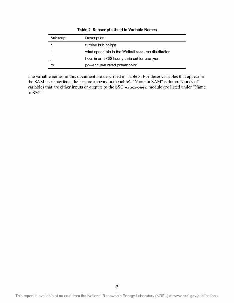
Table 2. Subscripts Used in Variable Names

Subscript Description

h turbine hub height

i wind speed bin in the Weibull resource distribution

j hour in an 8760 hourly data set for one year

m power curve rated power point The variable names in this document are described in Table 3. For those variables that appear in the SAM user interface, their name appears in the table's "Name in SAM" column. Names of variables that are either inputs or outputs to the SSC windpower module are listed under "Name in SSC."

3


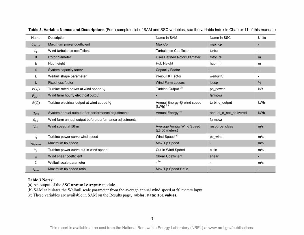
Table 3. Variable Names and Descriptions (For a complete list of SAM and SSC variables, see the variable index in Chapter 11 of this manual.)

Name Description Name in SAM Name in SSC Units

CPmax Maximum power coefficient Max Cp max_cp -

𝐶𝑡 Wind turbulence coefficient Turbulence Coefficient turbul -

D Rotor diameter User Defined Rotor Diameter rotor_di m

h Hub height Hub Height hub_ht m

K System capacity factor Capacity Factor - -

k Weibull shape parameter Weibull K Factor weibullK -

L Fixed loss factor Wind Farm Losses lossp %

𝑃(𝑉𝑖) Turbine rated power at wind speed 𝑉𝑖 Turbine Output (c) pc_power kW

𝑃𝑤𝑓,𝑗 Wind farm hourly electrical output - farmpwr

𝑄(𝑉𝑖) Turbine electrical output at wind speed 𝑉𝑖 Annual Energy @ wind speed (kWh) (c)

turbine_output kWh

𝑄𝑠𝑦𝑠 System annual output after performance adjustments Annual Energy (a) annual_e_net_delivered kWh

𝑄𝑤𝑓 Wind farm annual output before performance adjustments - farmpwr

V50 Wind speed at 50 m Average Annual Wind Speed (@ 50 meters)

resource_class m/s

𝑉𝑖 Turbine power curve wind speed Wind Speed (c) pc_wind m/s

Vtip max Maximum tip speed Max Tip Speed - m/s

𝑉0 Turbine power curve cut-in wind speed Cut-in Wind Speed cutin m/s

α Wind shear coefficient Shear Coefficient shear -

λ Weibull scale parameter - (b) - m/s

λmax Maximum tip speed ratio Max Tip Speed Ratio - -

Table 3 Notes: (a) An output of the SSC annualoutput module. (b) SAM calculates the Weibull scale parameter from the average annual wind speed at 50 meters input. (c) These variables are available in SAM on the Results page, Tables, Data: 161 values.

4


3 Introduction This reference manual describes the wind power performance model in the National Renewable Energy Laboratory's System Advisor Model (SAM) Version 2013.9.20 (SIL 3.0.1, SSC 33).

SAM is a desktop application designed for renewable energy analysts to evaluate system design and project financial options. SAM's wind power performance model is also available to software developers as the windpower module in the SAM Simulation Core (SSC) application programming interface (API) included in the SAM software development kit (SDK).

NREL provides both the SAM application and SDK for free from the SAM website at https://sam.nrel.gov/. More information about the software development tools can also be found on the SAM website.

For SAM users, this reference manual supplements the SAM user documentation in SAM's Help system.1 For software programmers, it supports development of applications that use the API to the windpower module.

3.1 SAM Overview

The System Advisor Model (SAM) is a desktop application designed to facilitate techno-economic analysis of renewable energy projects. It is a decision-making tool for project developers, financial analysts, policymakers, and energy researchers. SAM can model grid-connected power systems that use wind, photovoltaic, concentrating solar power, solar hot water, biopower, or geothermal electricity generation technologies.

To model a renewable energy project in SAM, you choose a performance model to represent the system, and a financial model to represent the project's financial structure. You then specify values on the input pages to describe the physical characteristics of the system and financial parameters of the project. All of the input variables are populated with default values so that you can start generating preliminary results before you have collected all of the data for your project. After specifying inputs, you run a simulation and the performance model makes a series of 8,760 hour-by-hour calculations to calculate the system's hourly electrical output over a one-year period2. The financial model uses the hourly electric generation profile and user inputs such as installation and operating costs, electricity price, taxes and incentives, and debt parameters to calculate the project's annual cash flows over a multi-year period [1]. SAM displays results from both the performance and the financial models in tables and graphs, and provides options for exporting the results for use in reports and presentations.

SAM's advanced simulation options facilitate parametric, sensitivity, and statistical studies that involve multiple simulation runs. The SamUL scripting language is a built-in programming language that makes it possible to automate repetitive or complex modeling tasks.

1 SAM's user documentation is available as a Help system in the user interface, and as both a web document and PDF document on the SAM website at https://sam.nrel.gov/content/resources-learning-sam (accessed October 11, 2013). 2 This description is generally true for SAM's performance models, with the exception of the wind power model's Weibull distribution option for the wind resource which calculates a statistical distribution of the system's annual output instead of time-series values (see Chapter 4.2).

https://sam.nrel.gov/

https://sam.nrel.gov/content/resources-learning-sam

5


SAM can model both distributed generation and central generation projects. The residential and commercial financial models are for distributed generation projects that buy and sell electricity at retail rates, and use renewable energy to supplement electricity from the grid to meet a building’s or facility's electric load. The utility financial models are for central generation projects that sell all of the electricity generated by the system at a price negotiated through a power purchase agreement.

This manual describes SAM's wind power performance model. It does not describe the financial models or other simulation options available in SAM. For an overview of SAM's financial models, see the Financial Models topic in SAM's Help system [https://www.nrel.gov/analysis/sam/help/html-php/index.html?fin_overview.htm].

3.2 SAM Simulation Core (SSC)

The SAM Simulation Core (SSC) is the library of software modules that SAM uses to run simulations. The SSC's application programming interface (API) makes it possible for software developers to develop their own applications using SAM's underlying performance and financial models.

The SAM Software Development Kit (SDK) is a collection of software development tools that make it possible to write programs in C++, C#, Java, MATLAB, or python that run SAM Simulation Core (SSC) modules. The SDK includes the API to the windpower simulation module described here, and the APIs to SAM's other modules. Note that the SDK does not provide access to the module's source code.

Table 3 and the Index of SAM and SSC Variable Names on Page 27 show where a specific windpower module variable is mentioned in this manual.

3.3 Model Applications and Limitations

SAM's performance models are intended for project pre-feasibility level analysis. The wind performance model can provide a very preliminary estimate of the expected hourly electricity production and capacity factor over a one-year period for a single wind turbine, small wind project, or large wind farm. The financial model uses the sum of the hourly values as an estimate of the project's production in its first year, and extends the estimate over a period of several years to calculate metrics such as levelized cost of energy, project net present value, power purchase agreement (PPA) price and internal rate of return for utility projects, and total electricity savings and payback period for residential and commercial projects.

SAM's wind performance model requires information that describes the wind resource at the project location, a set of inputs to describe the wind turbine performance characteristics, and inputs to describe the layout of the turbines for projects with more than one turbine. The quality of the performance model's predictions depends on the quality of these inputs.

SAM's approach to modeling a wind farm includes a number of simplifying assumptions described in Chapter 8. Although SAM does calculate wake effect losses due to the effect of upwind turbines on their downwind neighbors, more detailed wind analysis models are better suited than SAM for detailed analysis of the impact of farm layout, topography and terrain on wind farm performance.

6


SAM's hourly simulation time step provides enough temporal resolution to offer insight into the effect of daily and seasonal resource variation on the system's output with sufficient detail for project techno-economic modeling, but not for detailed engineering design modeling such as physical stresses on turbine components or electrical transients.

3.4 General Modeling Approach

The SAM wind performance model algorithm consists of the four primary steps described briefly below and in more detail in the chapters that follow.

Step 1. Characterize the Wind Resource: The wind power model uses wind resource data either from an hourly data file or defined as a Weibull statistical distribution.

Step 2. Specify the Wind Turbine's Power Curve: SAM models wind turbine performance using a power curve- either a user-specified power curve table or one that SAM calculates from a set of turbine characteristics.

Step 3. Define the Wind Farm Layout: The wind farm is a two-dimensional array of coordinates for each turbine's location with additional inputs used to calculate wake effect losses.

Step 4. Calculate the Wind Farm Electrical Output: SAM's hour-by-hour simulation calculates the system's electrical output in kWh for each of the 8,760 hours in one year.3 SAM reports the hourly values on the Results page along with monthly and annual totals in tables and graphs that can be exported to other applications.

4 Wind Resource Data Options The wind resource data provides information about the kinetic energy available in the wind at the wind turbine's location and hub height. The amount of available energy depends on the wind speed and air density and varies with time. The options on SAM's Wind Resource input page determine how SAM characterizes the wind resource:

• Weather file (Wind Resource by Location), Chapter 4.1: The wind resource data comes from a weather file with 8,760 hourly values for wind speed, direction, air temperature, and air pressure at one or more turbine hub heights.

• Weibull distribution (Wind Resource Characteristics), Chapter 4.2: The wind resource is represented by a statistical distribution characterized by an annual average wind speed value and Weibull K factor. This option only works with a single turbine because there is insufficient data to model wind farm wake effects.

In the SSC windpower module, variable model_choice = 0 is equivalent to the Wind Resource by Location option in SAM, and model_choice = 1 is equivalent to the Weibull distribution option.

3 The financial models assume that this annual generation profile applies to all years in the project life. They apply a set of optional performance adjustment factors to account for system availability, curtailment, and any annual decrease in system output. See the user documentation for details (or online at https://www.nrel.gov/analysis/sam/help/html-php/index.html?fin_annual_performance.htm, last visited October 10, 2013).

https://www.nrel.gov/analysis/sam/help/html-php/index.html?fin_annual_performance.htm

7


4.1 Wind Resource Data from a Weather File

When the option on SAM's Wind Resource input page is Wind Resource by Location, SAM reads wind resource data from the weather file highlighted in the weather file list. The Folder Settings options determine where on your computer SAM looks for the weather files.

In the SSC windpower module, the variable file_name stores the weather file’s complete path and name, for example file_name = "c:\users\paul\weather data\my_weather_file.srw" refers to a weather file named my_weather_file.srw in the c:\users\paul\weather\data folder.

4.1.1 The SRW Weather File Format The wind performance model reads wind resource data from a weather file in the SRW format4, which is a text format with comma-separated values. You can find examples SRW files in the default weather file folder (c:\SAM\2013.9.20\weather in Windows), and a description of the format in the "Weather File Formats" topic of SAM's help system [2].

The SRW file format is designed to be flexible enough to allow you to create files with your own data. See the SAM help topic for more information on using or creating SRW files.

4.1.2 Representative Typical Weather Files The SAM installation package includes a set of 39 weather files developed for NREL by AWS Truepower that contain wind speed, wind direction, ambient temperature, and atmospheric pressure data at 50, 80, and 110 meters above the ground. They are "representative" because they are for locations with topography and weather combinations that represent regions of the U.S. where large-scale wind farms are typically developed. The files are "typical" because they represent the wind resource over a period of 14 years between 1997 and2010 [3].

4.1.3 Weather Files from the NREL Wind Integration Datasets This data is available for 2004, 2005, and 2006 from different sources for the Western United States and Eastern United States. The Western Wind Dataset has data developed by NREL and 3Tier for over 32,000 locations in the Western United States. The Eastern Wind Data set has data developed by NREL and AWS Truepower for 1,326 locations in the Eastern United States. When you download data from these datasets from within SAM, SAM converts the data into an SRW file.

The Download weather file button on SAM's Wind Resource input page when it is in Wind Resource by Location mode automatically downloads files from the NREL Wind Integration Datasets database. The SSC windpower module does not have a function for accessing this database, but these files can be downloaded externally and used with the SSC module.

4.2 Wind Resource Data as a Weibull Distribution

For analyses that do not require the detail of time series wind resource data, SAM's Weibull distribution option represents the wind resource as a statistical distribution characterized by a single average annual wind speed and Weibull K factor. This option may be useful for very

4 Older versions of the model used a different file format than that used in the SRW file extension.

8


preliminary project feasibility studies before time series data is available, or for analyses involving parametric studies on a single annual average wind speed value or the shape of wind speed distribution over the year.

SAM disables the variables on SAM's Wind Farm input page with the Weibull Distribution wind resource option because the option provides no information about wind direction that SAM needs to model wake effect losses in a wind farm.

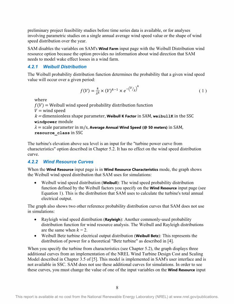
4.2.1 Weibull Distribution The Weibull probability distribution function determines the probability that a given wind speed value will occur over a given period:

𝑓(𝑉) = 𝑘𝜆𝑘 × (𝑉)𝑘−1 × 𝑒−�𝑉

𝜆� �𝑘

( 1 )

where 𝑓(𝑉) = Weibull wind speed probability distribution function 𝑉 = wind speed k = dimensionless shape parameter, Weibull K Factor in SAM, weibullK in the SSC windpower module 𝜆 = scale parameter in m/s, Average Annual Wind Speed (@ 50 meters) in SAM, resource_class in SSC

The turbine's elevation above sea level is an input for the "turbine power curve from characteristics" option described in Chapter 5.2. It has no effect on the wind speed distribution curve.

4.2.2 Wind Resource Curves When the Wind Resource input page is in Wind Resource Characteristics mode, the graph shows the Weibull wind speed distribution that SAM uses for simulations:

• Weibull wind speed distribution (Weibull): The wind speed probability distribution function defined by the Weibull factors you specify on the Wind Resource input page (see Equation 1). This is the distribution that SAM uses to calculate the turbine's total annual electrical output.

The graph also shows two other reference probability distribution curves that SAM does not use in simulations:

• Rayleigh wind speed distribution (Rayleigh): Another commonly-used probability distribution function for wind resource analysis. The Weibull and Rayleigh distributions are the same when 𝑘 = 2.

• Weibull Betz turbine electrical output distribution (Weibull Betz): This represents the distribution of power for a theoretical "Betz turbine" as described in [4].

When you specify the turbine from characteristics (see Chapter 5.2), the graph displays three additional curves from an implementation of the NREL Wind Turbine Design Cost and Scaling Model described in Chapter 3.5 of [5]. This model is implemented in SAM's user interface and is not available in SSC. SAM does not use these additional curves for simulations. In order to see these curves, you must change the value of one of the input variables on the Wind Resource input

9


page because the graph will only refresh when an input value changes (this behavior may change in future versions of SAM so that the graph updates automatically). The three curves are:

• Weibull coefficient of power turbine electrical output distribution (Weibull Cp): Distribution of the modeled electrical output of the turbine with characteristics defined on the Turbine input page.

• Turbine electrical output distribution (Turbine Energy): The product of the turbine power and the Weibull probability.

• Hub efficiency distribution (Hub Eff/10): The conversion efficiency of the turbine with characteristics defined on the Turbine input page. The efficiency value is divided by 10 so that it fits on the right-hand y-axis.

5 Wind Turbine Model Options SAM uses a wind turbine power curve to calculate the turbine's electrical output in each time step, given the resource characteristics as described above. The Turbine input page provides two options for defining the power curve:

• Power curve library (Select turbine from a list), Chapter 5.1: A pre-defined table of wind speed/turbine output value pairs represents the turbine's performance. When you choose a turbine from the list on the Turbine input page, SAM displays the turbine's power curve from the library.

• Turbine characteristics (Define the turbine characteristics below), Chapter 5.2: SAM uses a set of user-specified turbine design parameters to calculate a turbine power curve. You specify values for the parameters on the Turbine input page, and SAM calculates and displays the power curve.

5.1 Turbine Power Curve from the Library

SAM's power curve library contains power curve data developed by NREL for the NREL Wind Turbine Cost and Scaling Model described in [4]. NREL developed the power curves from analysis of published performance data, so they do not represent manufacturer data.

The power curve library is not part of the SSC windpower module. In the windpower module, you specify the wind turbine power curve using the pc_wind and pc_power input variables, where pc_wind is a list of wind speed values included in the power curve in m/s, and pc_power is a list of the same length containing the power curve output values in kW.

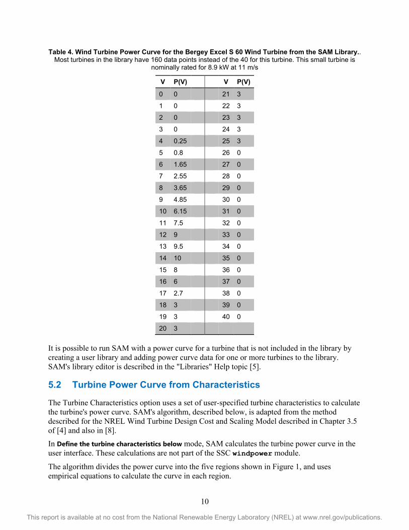
For most turbines in the library, SAM stores an array of 160 pairs of wind speed and power output values, corresponding to wind speeds in 0.25 m/s increments from 0 to 40 m/s. Table 4 shows an example from the library for a small wind turbine's power curve (note that unlike most turbines in the library, this turbine power curve has fewer than 160 value pairs).

10


Table 4. Wind Turbine Power Curve for the Bergey Excel S 60 Wind Turbine from the SAM Library.. Most turbines in the library have 160 data points instead of the 40 for this turbine. This small turbine is

nominally rated for 8.9 kW at 11 m/s

V P(V) V P(V)

0 0 21 3

1 0 22 3

2 0 23 3

3 0 24 3

4 0.25 25 3

5 0.8 26 0

6 1.65 27 0

7 2.55 28 0

8 3.65 29 0

9 4.85 30 0

10 6.15 31 0

11 7.5 32 0

12 9 33 0

13 9.5 34 0

14 10 35 0

15 8 36 0

16 6 37 0

17 2.7 38 0

18 3 39 0

19 3 40 0

20 3 It is possible to run SAM with a power curve for a turbine that is not included in the library by creating a user library and adding power curve data for one or more turbines to the library. SAM's library editor is described in the "Libraries" Help topic [5].

5.2 Turbine Power Curve from Characteristics

The Turbine Characteristics option uses a set of user-specified turbine characteristics to calculate the turbine's power curve. SAM's algorithm, described below, is adapted from the method described for the NREL Wind Turbine Design Cost and Scaling Model described in Chapter 3.5 of [4] and also in [8].

In Define the turbine characteristics below mode, SAM calculates the turbine power curve in the user interface. These calculations are not part of the SSC windpower module.

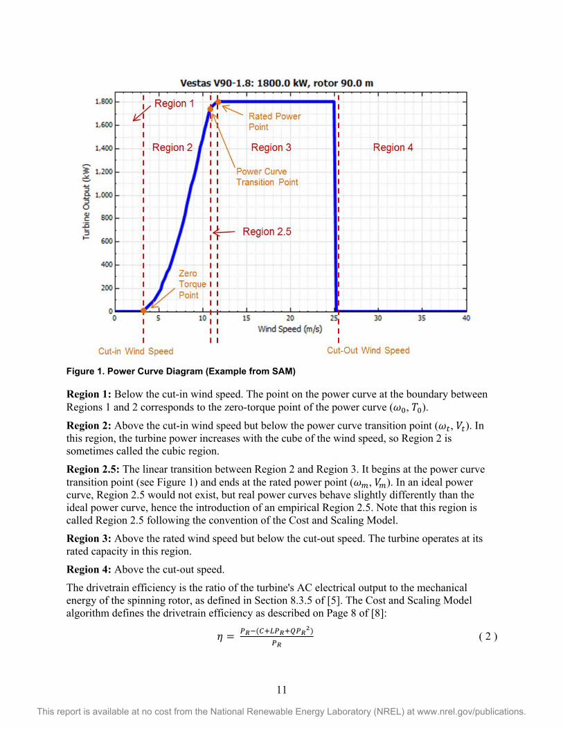
The algorithm divides the power curve into the five regions shown in Figure 1, and uses empirical equations to calculate the curve in each region.

11


Figure 1. Power Curve Diagram (Example from SAM)

Region 1: Below the cut-in wind speed. The point on the power curve at the boundary between Regions 1 and 2 corresponds to the zero-torque point of the power curve (𝜔0, 𝑇0).

Region 2: Above the cut-in wind speed but below the power curve transition point (𝜔𝑡, 𝑉𝑡). In this region, the turbine power increases with the cube of the wind speed, so Region 2 is sometimes called the cubic region.

Region 2.5: The linear transition between Region 2 and Region 3. It begins at the power curve transition point (see Figure 1) and ends at the rated power point (𝜔𝑚, 𝑉𝑚). In an ideal power curve, Region 2.5 would not exist, but real power curves behave slightly differently than the ideal power curve, hence the introduction of an empirical Region 2.5. Note that this region is called Region 2.5 following the convention of the Cost and Scaling Model.

Region 3: Above the rated wind speed but below the cut-out speed. The turbine operates at its rated capacity in this region.

Region 4: Above the cut-out speed.

The drivetrain efficiency is the ratio of the turbine's AC electrical output to the mechanical energy of the spinning rotor, as defined in Section 8.3.5 of [5]. The Cost and Scaling Model algorithm defines the drivetrain efficiency as described on Page 8 of [8]:

𝜂 = 𝑃𝑅−(𝐶+𝐿𝑃𝑅+𝑄𝑃𝑅2)

𝑃𝑅 ( 2 )

12


where 𝜂 = drivetrain efficiency 𝐶 = constant turbine losses 𝐿 = linear turbine losses 𝑄 = quadratic turbine losses 𝑃𝑅 = power ratio (ratio of produced power to rated power)

Constant losses are independent of power production and include transformer losses and other electrical conversion losses. Linear losses scale directly with power production. Quadratic losses depend on the square of the power production. The most common quadratic loss is copper losses at constant voltage (resulting from the well-known 𝑃 = 𝐼2𝑅 equation, where 𝐼 is current and 𝑅 is resistance). The losses are dependent on the type of drive train as shown in Table 5 [8].

The algorithm assumes an ideal power ratio of one, 𝑃𝑅 = 1, so that Equation 2 simplifies to:

𝜂 = 1 − (𝐶 + 𝐿 + 𝑄) ( 3 )

Table 5. Drivetrain loss characteristics by drivetrain design

Drivetrain Design C L Q Total Losses

3 Stage Planetary 0.013 0.085 0 0.098

Single Stage 0.013 0.037 0.061 0.11

Multi-Generator 0.015 0.044 0.058 0.12

Direct Drive 0.010 0.020 0.069 0.099

The rated hub power is given by:

𝑃h,m = 𝑃m𝜂

( 4 )

where 𝑃h,m = calculated rated hub power in W 𝑃m = turbine rated power in W, User Defined Rated Output on the Turbine input page 𝜂 = drivetrain efficiency

And the rated hub rotor speed is:

𝜔𝑚 = 2𝑉𝑡𝑖𝑝 𝑚𝑎𝑥

𝐷 ( 5 )

where 𝜔𝑚 = rated hub rotor speed in revolutions per second 𝑉𝑡𝑖𝑝 𝑚𝑎𝑥 = maximum tip speed in m/s, Max Tip Speed on the Turbine input page 𝐷 = rotor diameter in m, User Defined Rotor Diameter in SAM

The rated torque 𝑇𝑚 in N‐m is then:

𝑇𝑚 = 𝑃h,m𝜔𝑚

( 6 )

13


The calculations for power curve regions 2.5, 3, and 4 require another parameter, the variable speed torque constant [4]:

𝑘 = 𝜋𝜌𝐷5𝐶𝑃𝑚𝑎𝑥64𝜆𝑚𝑎𝑥

3 ( 7 )

where 𝑘 = variable speed torque constant in kg*m2 𝐶𝑃𝑚𝑎𝑥 = maximum turbine coefficient of power, Max Cp on the Turbine input page 𝜆𝑚𝑎𝑥 = the maximum tip speed ratio, Max Tip Speed Ratio in SAM 𝜌 = air density in kg/m3, from Equation 8

The air density at any altitude is:

𝜌 = 𝑝0×�1−𝐿𝑏×s

𝑇0�

𝑔0𝐿𝑏 ×𝑅𝑠𝑝

𝑅𝑠𝑝×(𝑇0+𝐿𝑏×𝑠) ( 8 )

where 𝑝0 = mean sea level atmospheric pressure (101,325 Pa) 𝐿𝑏 = standard temperature lapse rate (‐0.0065 K/m) 𝑠 = elevation above sea level in meters, either from the weather file, or Elevation Above Mean Sea Level on the Wind Resource input page 𝑇0 = ICAO standard temperature (288.15 K) 𝑔0 = standard gravity (9.80665 m/s2) 𝑅𝑠𝑝= specific gas constant for dry air (287.058 J/kg∙K)

The transition points between power curve regions are the zero torque point, power curve transition point, rated power point, and cut-out wind speed (given in turbine specifications) shown in Figure 1.

The Region 2 rotor speed where torque is zero is given by:

𝜔0 = 𝜔𝑚1+ 𝑚

100% ( 9 )

where 𝜔0 = rotor speed at zero torque 𝜔𝑚 = rotor speed at rated torque, from Equation 5 𝑚 = the slope of Region 2.5 of the power curve, assumed to be 5%

The sloped sections of the power curve in Region 2 and Region 2.5 intersect at the power curve transition point:

𝜔𝑡 = −𝑏−√𝑏2−4𝑎𝑐2𝑎

( 10 )

14


where 𝜔𝑡 = rotor speed at transition point 𝑎 = 𝑘 from Equation 7

𝑏 = −𝑇𝑚

𝜔𝑚 − 𝜔0

𝑐 = 𝑇𝑚𝜔0

𝜔𝑚 − 𝜔0

The wind speed in m/s at the transition point is:

𝑉𝑡 = 𝜔𝑡𝐷2𝜆𝑚𝑎𝑥

( 11 )

And the power in W at the transition point is:

𝑃𝑡 = 𝑘𝜔𝑡3 ( 12 )

The wind speed at the rated power point in m/s is given by:

𝑉𝑟 = 13

� 2𝑃h,m

𝜌𝜋𝐷24 𝐶𝑃𝑚𝑎𝑥

�1/3

+ 23

� 1

1.5𝜌𝜋𝐷24 𝐶𝑃𝑚𝑎𝑥𝑉𝑡

2× �𝑃h,m − 𝑃𝑡� + 𝑉𝑡� ( 13 )

The derivation of Equation 13 is beyond the scope of this manual.

After calculating values for the transition points, the Cost and Scaling Model algorithm calculates hub power and wind speed value pairs to define the entire power curve for wind speeds between 0 and 40 m/s in increments of 0.25 m/s. The hub power calculation used at each speed depends on the region in which that wind speed falls, which may be determined from comparison to the transition points.

For Regions 1 and 4 (below cut-in speed and above cut-out speed, respectively), the hub power is zero by definition:

𝑃ℎ = 0 ( 14 )

In Region 2, hub power is a cubic function of the wind speed:

𝑃ℎ = 𝑘1000

�𝑉𝜆𝑚𝑎𝑥𝐷

2��

3 ( 15 )

where 𝑃ℎ = hub power at wind speed 𝑉 𝑘 = variable speed torque constant from Equation 7 𝜆𝑚𝑎𝑥 = maximum tip speed ratio, Max Tip Speed Ratio from the Turbine input page 𝐷 = rotor diameter, User Defined Rotor Diameter from SAM

In Region 2.5, the hub power at a given wind speed 𝑉 is interpolated linearly between 𝑉𝑡 and 𝑉𝑟 calculated in Equations 11 and 13, respectively:

𝑃ℎ = (𝑉−𝑉𝑡)(𝑉𝑟−𝑉𝑡)

(𝑃h,m − 𝑃𝑡) + 𝑃𝑡 ( 16 )

In Region 3, the hub power is equal to the rated power:

15


𝑃ℎ = 𝑃h,m ( 17 )

The Cost and Scaling Model algorithm can now calculate the actual drivetrain efficiency 𝜂 at wind speed 𝑉 for non-zero hub power 𝑃ℎ using the actual power ratio, rather than the ideal power ratio used in Equation 2:

𝜂 = � 𝑃ℎ

𝑃h,m�−�𝐶+𝐿 𝑃ℎ

𝑃h,m+𝑄� 𝑃ℎ

𝑃h,m�

2�

� 𝑃ℎ𝑃h,m

� ( 18 )

Combining the appropriate equation from Equations 14-16 with Equation 18, the turbine power at any wind speed 𝑉 is then:

𝑃 = 𝑃ℎ𝜂 ( 19 )

SAM stores these turbine power values in an array of 160 points corresponding to their wind speeds, similar to the power curve of a library turbine. The values are available in SAM after running simulations on the Results page, in Tables, under Data: 161 values as Turbine Power Curve - Rating (kW) and Turbine Power Curve - Wind Speed (m/s).

6 Wind Turbine Output from a Weibull Distribution When you run a simulation in SAM with the wind resource defined as a Weibull distribution or the SSC windpower module with model_choice = 1 (see Chapter 4), SAM does not perform a time series simulation, but instead calculates the turbine's electrical output for a series of wind speed “bins.” Each bin is a range of wind speeds on the turbine power curve from the current wind speed (𝑉𝑖) to the previous wind speed (𝑉𝑖−1).

The number of bins depends on the wind turbine model. Most power curves in SAM's turbine library have 160 wind speed points (every 0.25 m/s from 0-40 m/s), which corresponds to 160 wind speed bins. Some of the turbines in the library have fewer points. When SAM calculates the power curve from turbine characteristics, it uses 160 points.

When you specify the wind resource as a Weibull distribution, there is no information about wind direction, so SAM disables the wind farm inputs and models the system as a single turbine.

6.1 Wind Speed at Turbine Hub Height

To compute the power output for a given wind speed bin, SAM first determines the wind speed at the turbine hub height:

𝑉ℎ = 𝑉50 � ℎ50

�𝛼

( 20 )

16


where 𝑉ℎ = wind speed at the hub height in m/s 𝑉50 = wind speed at 50 m in m/s, Average Annual Wind Speed (@ 50 meters) on the Wind Resource input page ℎ = hub height in m, Hub Height on the Turbine input page 𝛼 = shear coefficient, Shear Coefficient on the Turbine input page

The shear coefficient depends on the terrain, typically ranging from about 0.1 for open water to about 0.3 for hills or mountains. Because 𝑉ℎ describes the average wind speed of the Weibull distribution for the given hub height, the shape parameter for that hub height can be back-calculated using the gamma function 𝛤 [6]:

𝜆ℎ = 𝑉ℎ

𝑒log 𝛤�1+1𝑘�

( 21 )

where 𝜆ℎ = Weibull shape parameter (unitless) at hub height ℎ 𝑉ℎ = average wind speed in m/s at hub height ℎ 𝑘 = Weibull k parameter, Weibull K Factor on the Wind Resource input page, WeibullK in the SSC windpower module

6.2 Wind Speed Probability

Next, SAM uses the cumulative probability distribution function to predict the probability that the turbine hub wind speed will be a positive number less than or equal to the wind speed 𝑉𝑖 (note that the cumulative distribution function is different from the probability distribution function in Equation 1):

𝐹(𝑉𝑖) = 1 − 𝑒−(

𝑉𝑖𝜆ℎ

)𝑘 ( 22 )

where 𝐹(𝑉𝑖) = Weibull cumulative probability distribution function for wind speed 𝑉𝑖 = wind speed in m/s 𝑘 = Weibull k factor, Weibull K Factor on the Wind Resource input page 𝜆ℎ= shape parameter at hub‐height ℎ from Equation 21

The probability that the hub wind speed will fall within the current wind speed bin is given by:

𝐹(𝑏𝑖𝑛) = 𝐹(𝑉𝑖) − 𝐹(𝑉𝑖−1) ( 23 )

where 𝐹(𝑉𝑖) and 𝐹(𝑉𝑖−1) = the cumulative probability function at the wind speed in the current bin and previous bin, respectively.

6.3 Turbine Output Probability

Finally, to compute the contribution of this wind speed bin to the total annual electrical output, SAM computes the power for wind speed bin i:

17


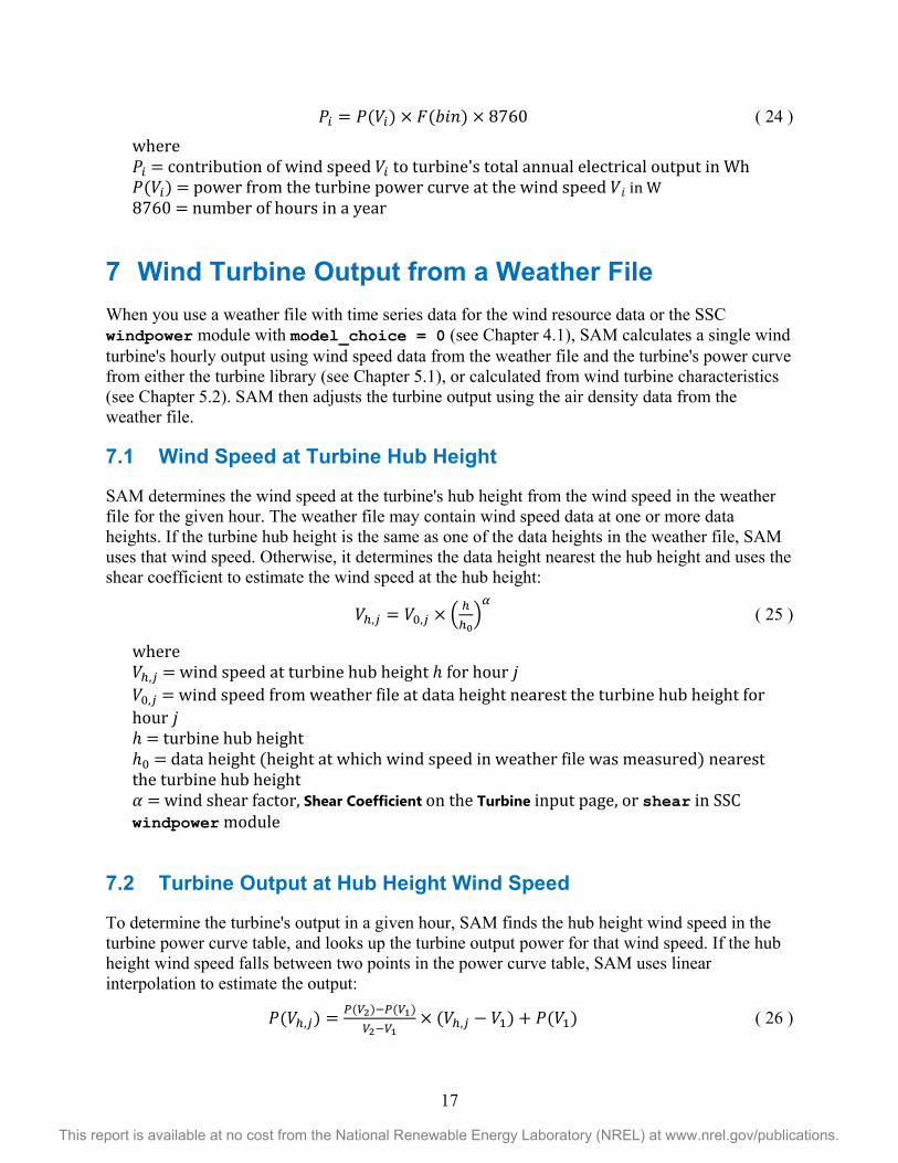
𝑃𝑖 = 𝑃(𝑉𝑖) × 𝐹(𝑏𝑖𝑛) × 8760 ( 24 )

where 𝑃𝑖 = contribution of wind speed 𝑉𝑖 to turbine's total annual electrical output in Wh 𝑃(𝑉𝑖) = power from the turbine power curve at the wind speed 𝑉𝑖 in W 8760 = number of hours in a year

7 Wind Turbine Output from a Weather File When you use a weather file with time series data for the wind resource data or the SSC windpower module with model_choice = 0 (see Chapter 4.1), SAM calculates a single wind turbine's hourly output using wind speed data from the weather file and the turbine's power curve from either the turbine library (see Chapter 5.1), or calculated from wind turbine characteristics (see Chapter 5.2). SAM then adjusts the turbine output using the air density data from the weather file.

7.1 Wind Speed at Turbine Hub Height

SAM determines the wind speed at the turbine's hub height from the wind speed in the weather file for the given hour. The weather file may contain wind speed data at one or more data heights. If the turbine hub height is the same as one of the data heights in the weather file, SAM uses that wind speed. Otherwise, it determines the data height nearest the hub height and uses the shear coefficient to estimate the wind speed at the hub height:

𝑉ℎ,𝑗 = 𝑉0,𝑗 × � ℎℎ0

�𝛼

( 25 )

where 𝑉ℎ,𝑗 = wind speed at turbine hub height ℎ for hour 𝑗 𝑉0,𝑗 = wind speed from weather file at data height nearest the turbine hub height for hour 𝑗 ℎ = turbine hub height ℎ0 = data height (height at which wind speed in weather file was measured) nearest the turbine hub height 𝛼 = wind shear factor, Shear Coefficient on the Turbine input page, or shear in SSC windpower module

7.2 Turbine Output at Hub Height Wind Speed

To determine the turbine's output in a given hour, SAM finds the hub height wind speed in the turbine power curve table, and looks up the turbine output power for that wind speed. If the hub height wind speed falls between two points in the power curve table, SAM uses linear interpolation to estimate the output:

𝑃(𝑉ℎ,𝑗) = 𝑃(𝑉2)−𝑃(𝑉1)𝑉2−𝑉1

× (𝑉ℎ,𝑗 − 𝑉1) + 𝑃(𝑉1) ( 26 )

18


where 𝑃�𝑉ℎ,𝑗� = turbine output at hub height wind speed for hour 𝑗 𝑉ℎ,𝑗 = hub height wind speed for hour 𝑗 𝑃(𝑉) = the turbine output at wind speed V from the power curve 𝑉1 and 𝑉2 = the next smallest and largest power curve wind speed to the hub height wind speed, respectively

If the wind speed at hub height 𝑉ℎ,𝑗 for a given hour 𝑗 is less than the power curve cut-in speed, or greater than the highest wind speed in the power curve, then the turbine output 𝑃𝑗 is set to zero. Note that for most of the turbines in SAM's turbine library, the maximum wind speed is 40 m/s, and the cut-out wind speed is between 20 m/s and 25 m/s. For typical wind project locations in the United States, the maximum hourly average wind speed rarely exceeds 25 m/s.

7.3 Turbine Output Adjusted for Air Density

SAM assumes that the wind turbine power curve is for a turbine installed at sea level. The model adjusts turbine output at hub height wind speed for a given hour to the air density at the turbine's location in that hour. The hourly air density depends on the atmospheric pressure value from the weather file:

𝜌𝑗 = 𝑝𝑗

𝑅𝑠𝑝×𝑇𝑗 ( 27 )

where 𝜌𝑗= air density at the turbine location for hour 𝑗 𝑝𝑗 = atmospheric pressure at the turbine location from the weather file for hour 𝑗 converted from atm to Pa 𝑅𝑠𝑝= specific gas constant for dry air (287.058 J/kg∙K) 𝑇𝑗 = temperature from weather file for hour j converted from °C to K

The adjusted wind turbine output in W in a given hour is:

Pj = P�Vh,j� × ρj

ρ0 ( 28 )

where 𝑉𝑗 = the wind speed at hour j from the weather file 𝑃(𝑉ℎ,𝑗) = the turbine output at wind speed 𝑉ℎ,𝑗 from the turbine's power curve (calculated in Equation 26 above) 𝜌𝑗 = the air density at hour j from the weather file 𝜌0 = the air density at sea level, 1.225 kg/m3 at 15 °C

8 Wind Farm Output from a Weather File When you use a weather file with time series data for the wind resource data, SAM can model either a single wind turbine or a wind farm with two or more turbines.

19


Because SAM needs information about wind direction to calculate wake losses associated with a wind farm, it cannot model a multi-turbine wind farm when the wind resource data is defined by a Weibull distribution.

SAM makes the following simplifying assumptions about the wind farm:

• All turbines are at the same elevation above sea level so that the air density is constant across the entire wind farm.

• The terrain type is the same across the entire wind farm so that the wind shear is the same for all turbines.

When you model a wind farm with more than one turbine, SAM calculates the wind farm output for each hour using an algorithm conceptually similar to these steps:

1) Calculate the output and thrust coefficient of the most upwind turbine in the wind farm.

2) For each remaining turbine in the farm: a) Determine the downwind and crosswind distance from the nearest upwind

turbine using wind direction data from the weather file and turbine coordinates from the wind farm layout matrix.

b) Use the wake effect model to calculate the wind speed at the turbine using the output wind speed from the neighboring upwind turbine.

c) Calculate the turbine's electrical output and thrust coefficient at the adjusted wind speed.

3) Calculate the wind farm output by adding up the electrical output values of all the turbines.

4) Adjust the wind farm output by the wind farm loss factor.

8.1 Wind Farm Layout Matrix

In order to identify the upwind and downwind turbines in the wind farm, SAM uses a simple two-dimensional array to represent turbine locations. Each turbine location is an x,y coordinate pair that defines the distance in meters of the turbine from an arbitrary origin (0,0) where the smallest or most negative x and y values define the location of the southwest corner of a cardinally-oriented rectangle enclosing the wind farm.

The Wind Farm input page has a basic visual layout tool to help you specify the location of turbines using a rectangular or triangular layout. The input page also allows you to import wind turbine coordinates from a text file instead of using the layout tool. The layout tool and file format are both described in the Help topic for the Wind Farm input page [9].

In the SSC windpower module, you specify the rectangular coordinates of the turbine locations using two one-dimensional array variables: wt_x for the x-axis and wt_y for the y-axis location, where wt_x = 0 and wt_y = 0 is the origin as defined above, with distance from the origin measured in meters. The wind farm layout is independent of latitude and longitude information, and does not check for reasonability with respect to bodies of water, etc.

20


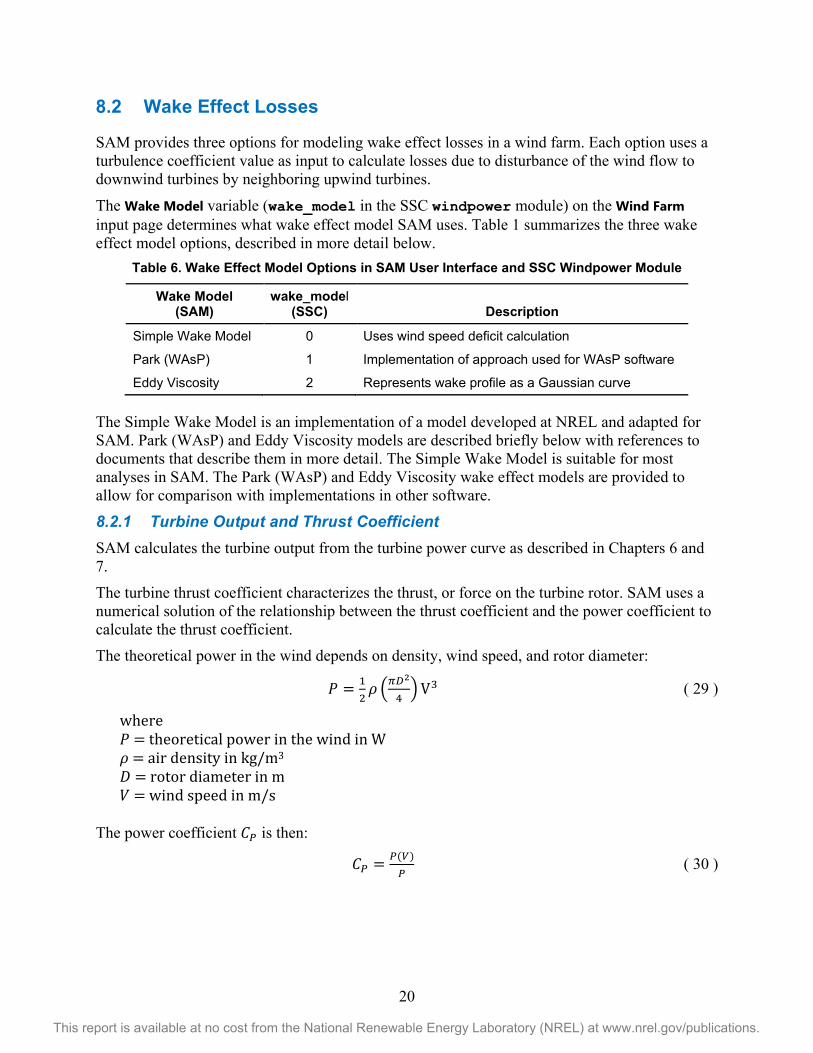
8.2 Wake Effect Losses

SAM provides three options for modeling wake effect losses in a wind farm. Each option uses a turbulence coefficient value as input to calculate losses due to disturbance of the wind flow to downwind turbines by neighboring upwind turbines.

The Wake Model variable (wake_model in the SSC windpower module) on the Wind Farm input page determines what wake effect model SAM uses. Table 1 summarizes the three wake effect model options, described in more detail below.

Table 6. Wake Effect Model Options in SAM User Interface and SSC Windpower Module

Wake Model (SAM)

wake_model (SSC)

Description

Simple Wake Model 0 Uses wind speed deficit calculation

Park (WAsP) 1 Implementation of approach used for WAsP software

Eddy Viscosity 2 Represents wake profile as a Gaussian curve The Simple Wake Model is an implementation of a model developed at NREL and adapted for SAM. Park (WAsP) and Eddy Viscosity models are described briefly below with references to documents that describe them in more detail. The Simple Wake Model is suitable for most analyses in SAM. The Park (WAsP) and Eddy Viscosity wake effect models are provided to allow for comparison with implementations in other software.

8.2.1 Turbine Output and Thrust Coefficient SAM calculates the turbine output from the turbine power curve as described in Chapters 6 and 7.

The turbine thrust coefficient characterizes the thrust, or force on the turbine rotor. SAM uses a numerical solution of the relationship between the thrust coefficient and the power coefficient to calculate the thrust coefficient.

The theoretical power in the wind depends on density, wind speed, and rotor diameter:

𝑃 = 12

𝜌 �𝜋𝐷2

4� V3 ( 29 )

where 𝑃 = theoretical power in the wind in W 𝜌 = air density in kg/m3

𝐷 = rotor diameter in m 𝑉 = wind speed in m/s

The power coefficient 𝐶𝑃 is then:

𝐶𝑃 = 𝑃(𝑉)𝑃

( 30 )

21


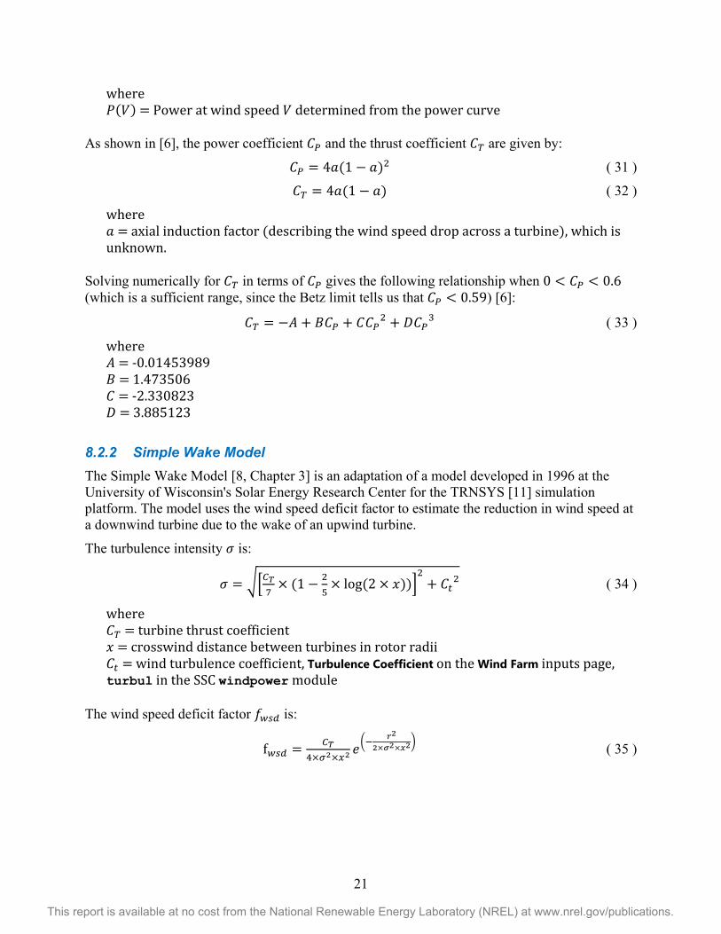
where 𝑃(𝑉) = Power at wind speed 𝑉 determined from the power curve

As shown in [6], the power coefficient 𝐶𝑃 and the thrust coefficient 𝐶𝑇 are given by:

𝐶𝑃 = 4𝑎(1 − 𝑎)2 ( 31 )

𝐶𝑇 = 4𝑎(1 − 𝑎) ( 32 )

where 𝑎 = axial induction factor (describing the wind speed drop across a turbine), which is unknown.

Solving numerically for 𝐶𝑇 in terms of 𝐶𝑃 gives the following relationship when 0 < 𝐶𝑃 < 0.6 (which is a sufficient range, since the Betz limit tells us that 𝐶𝑃 < 0.59) [6]:

𝐶𝑇 = −𝐴 + 𝐵𝐶𝑃 + 𝐶𝐶𝑃2 + 𝐷𝐶𝑃

3 ( 33 )

where 𝐴 = ‐0.01453989 𝐵 = 1.473506 𝐶 = ‐2.330823 𝐷 = 3.885123

8.2.2 Simple Wake Model The Simple Wake Model [8, Chapter 3] is an adaptation of a model developed in 1996 at the University of Wisconsin's Solar Energy Research Center for the TRNSYS [11] simulation platform. The model uses the wind speed deficit factor to estimate the reduction in wind speed at a downwind turbine due to the wake of an upwind turbine.

The turbulence intensity 𝜎 is:

𝜎 = ��𝐶𝑇7

× (1 − 25

× log (2 × 𝑥))�2

+ 𝐶𝑡2 ( 34 )

where 𝐶𝑇 = turbine thrust coefficient 𝑥 = crosswind distance between turbines in rotor radii 𝐶𝑡 = wind turbulence coefficient, Turbulence Coefficient on the Wind Farm inputs page, turbul in the SSC windpower module

The wind speed deficit factor 𝑓𝑤𝑠𝑑 is:

f𝑤𝑠𝑑 = 𝐶𝑇4×𝜎2×𝑥2 𝑒�− 𝑟2

2×𝜎2×𝑥2� ( 35 )

22


where C𝑇 = turbine power coefficient 𝜎 = transverse turbulence intensity (Equation 37) 𝑥 = downwind distance between turbines in number of rotor radii 𝑟 = crosswind distance between turbines in number of rotor radii

The adjusted wind speed 𝑉𝑎𝑑𝑗 is then:

𝑉𝑎𝑑𝑗 = V × (1 − f𝑤𝑠𝑑) ( 36 )

where 𝑉 = wind speed at neighboring upwind turbine 𝑓𝑤𝑠𝑑 = wind speed deficit factor (Equation 40)

8.2.3 Park Wake Model The Park wake model [12] assumes that a decrease in free-stream wind speed occurs immediately behind the turbine, and that the turbine wake expands linearly downstream of the turbine, with the magnitude of this expansion given by an empirically determined wake-decay constant k. Given the geometry shown in Figure 2:

Figure 2. Geometry of the Park Wake Model

The radius 𝑟𝑤 of the wake at the location of turbine 1 is computed using the wake-decay constant:

𝑟𝑤 = 𝐷02

+ 𝑘𝑋01 ( 37 )

where 𝐷0 = rotor diameter of the upstream turbine k = wake‐decay constant (in SAM, this is equal to 0.07, a typical value for this constant) 𝑋01 = horizontal distance between the upstream and downstream turbines

𝐴𝑜𝑣𝑒𝑟𝑙𝑎𝑝 is then computed geometrically. The decrease in wind speed occurring at the downstream turbine is then given by the wind speed deficit, calculated in the following:

𝛿𝑉 = �1 − �1 − 𝐶𝑇� � 𝐷0𝐷0+2𝑘𝑋01

�2 𝐴𝑜𝑣𝑒𝑟𝑙𝑎𝑝

𝐴1 ( 38 )

23


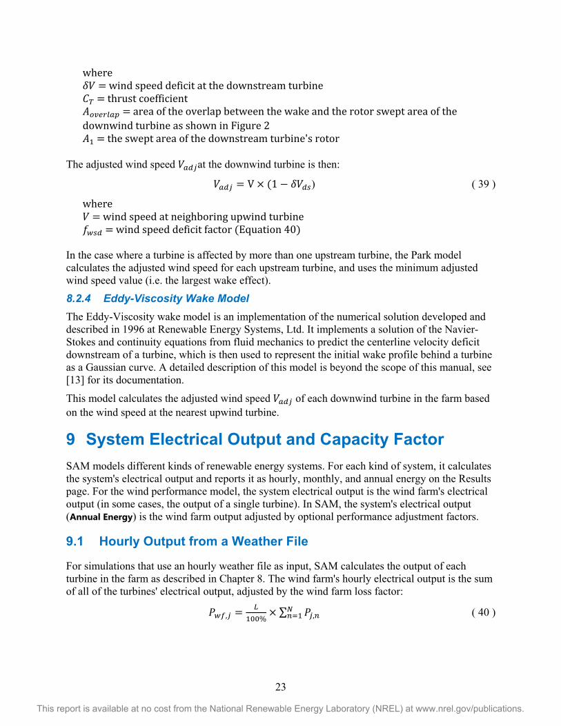
where 𝛿𝑉 = wind speed deficit at the downstream turbine 𝐶𝑇 = thrust coefficient 𝐴𝑜𝑣𝑒𝑟𝑙𝑎𝑝 = area of the overlap between the wake and the rotor swept area of the downwind turbine as shown in Figure 2 𝐴1 = the swept area of the downstream turbine's rotor

The adjusted wind speed 𝑉𝑎𝑑𝑗at the downwind turbine is then:

𝑉𝑎𝑑𝑗 = V × (1 − 𝛿𝑉𝑑𝑠) ( 39 )

where 𝑉 = wind speed at neighboring upwind turbine 𝑓𝑤𝑠𝑑 = wind speed deficit factor (Equation 40)

In the case where a turbine is affected by more than one upstream turbine, the Park model calculates the adjusted wind speed for each upstream turbine, and uses the minimum adjusted wind speed value (i.e. the largest wake effect).

8.2.4 Eddy-Viscosity Wake Model The Eddy-Viscosity wake model is an implementation of the numerical solution developed and described in 1996 at Renewable Energy Systems, Ltd. It implements a solution of the Navier-Stokes and continuity equations from fluid mechanics to predict the centerline velocity deficit downstream of a turbine, which is then used to represent the initial wake profile behind a turbine as a Gaussian curve. A detailed description of this model is beyond the scope of this manual, see [13] for its documentation.

This model calculates the adjusted wind speed 𝑉𝑎𝑑𝑗 of each downwind turbine in the farm based on the wind speed at the nearest upwind turbine.

9 System Electrical Output and Capacity Factor SAM models different kinds of renewable energy systems. For each kind of system, it calculates the system's electrical output and reports it as hourly, monthly, and annual energy on the Results page. For the wind performance model, the system electrical output is the wind farm's electrical output (in some cases, the output of a single turbine). In SAM, the system's electrical output (Annual Energy) is the wind farm output adjusted by optional performance adjustment factors.

9.1 Hourly Output from a Weather File

For simulations that use an hourly weather file as input, SAM calculates the output of each turbine in the farm as described in Chapter 8. The wind farm's hourly electrical output is the sum of all of the turbines' electrical output, adjusted by the wind farm loss factor:

𝑃𝑤𝑓,𝑗 = 𝐿100%

× ∑ 𝑃𝑗,𝑛𝑁𝑛=1 ( 40 )

24


where 𝑃𝑤𝑓,𝑗 = electrical output of wind farm in hour 𝑗 in kWh/h, in the SSC windpower module, farmpwr. (This value is not displayed on SAM's Results page.) 𝐿 = loss factor, Wind Farm Losses on the Wind Farm input page, lossp in the SSC windpower module 𝑃𝑗,𝑛 = electrical output of turbine 𝑛 in hour 𝑗 in kWh/h 𝑁 = number of turbines in the wind farm

The wind farm loss factor is intended to account for wiring and other losses associated with the wind farm design. You can account for operational losses such as system availability, curtailment, and degradation using the adjustment factors described in Section 9.3.

9.2 Annual Output Energy from a Weibull Distribution

For simulations based on a Weibull distribution of wind speed, SAM calculates each wind speed bin's contribution to the annual electrical energy output of a single turbine as described in Chapter 6. For a wind farm consisting of a single wind turbine, the annual electrical output is then:

𝑄𝑤𝑓 = ∑ 𝑃𝑖𝑁𝑖=1 ( 41 )

where 𝑄𝑤𝑓 = annual output of a single turbine in kWh 𝑃𝑖 = power output of the wind speed bin as shown in Equation 24 in kW 𝑁 = number of wind speed bins in the Weibull distribution

Recall that 𝑃𝑖 is already adjusted by the number of hours that it occurs per year, as shown in Equation 24.

Because SAM's financial models require hourly electrical output values, SAM calculates the values by dividing the annual electrical output by the number of hours in one year:

𝑃𝑤𝑓,𝑗 = 𝑄𝑤𝑓

8760 ( 42 )

where 𝑃𝑤𝑓,𝑗 = electrical output of the turbine in hour 𝑗 in kWh/h 𝑄𝑤𝑓 = annual output of a single turbine 8760 = number of hours in a year

9.3 Performance-Adjusted System Output

SAM applies a set of adjustment factors to the performance model's results to account for operational losses due to maintenance downtimes, grid operator curtailment requirements, or annual output degradation due to aging of system components. These factors are inputs on the Performance Adjustment input page. In SSC, these adjustment factors are not part of the windpower module. They are in the annualoutput module, and can use windpower module outputs as inputs.

25


The performance adjustment factors are (see [14] for more details):

• The Percent of annual output factor (energy_availability in the SSC annualoutput module) is applied to the wind farm (or turbine) annual output.

• The Year-to-year decline in output factor (energy_degradation in SSC) is applied to the annual output in Years 2 and later of the project cash flow.

• The Hourly Factors (energy_curtailment in SSC) are applied to the hourly output.

SAM reports the hourly, monthly, and annual energy values in results both before and after the performance adjustment factors.

9.4 System Annual Electrical Output (Annual Energy)

The system's annual electrical output is the sum of the turbines' output adjusted by the performance adjustment factors described in Section 13.3. SAM reports this value on the Results page as Annual Energy:

𝑄𝑠𝑦𝑠 = ∑ �𝑃𝑤𝑓,𝑗 × 𝐹𝑎𝑑𝑗,𝑗�8760𝑛=1 ( 43 )

where 𝑄𝑠𝑦𝑠 = adjusted annual electrical energy output of the system in kWh. (In SSC, this value can be calculated using the annualoutput module.) 𝑃𝑤𝑓,𝑗 = electrical output of wind farm in hour 𝑗 in kWh/h, in the SSC windpower module, farmpwr 𝐹𝑎𝑑𝑗,𝑗 = hourly adjustment factor defined on the Performance Adjustment input page in SAM, and in the SSC annualoutput module

9.5 Capacity Factor

The system's capacity factor is the ratio of the system's annual electrical output to its potential output at the wind farm's rated capacity:

𝐾 = 𝑄𝑠𝑦𝑠

𝑃m×8760 ( 44 )

where 𝐾 = system capacity factor 𝑄 = system's total annual electrical ouput in kWh after performance adjustments 𝑃𝑚 = wind farm's rated capacity in kW, System Nameplate Capacity on the Wind Farm input page 8760 = number of hours in one year

10 Summary The wind power model described in this manual is an hourly simulation model developed and distributed by the National Renewable Energy Laboratory that calculates a wind power system's hourly electrical output. The model is available for project modelers as part of the System

26


Advisor Model, and for software developers as the windpower module in the SAM Simulation Core software development kit. The model can simulate the performance of a single wind turbine or wind farm using weather data from a weather file or specified as a Weibull distribution. The model uses a wind turbine power curve to calculate the electrical output of a single turbine. For simulations of a wind farm, the model adjusts the output of each turbine in the farm using a wake effect model. A set of performance adjustment factors account for project operating losses.

27


11 Index of SAM and SSC Variable Names This index lists the page numbers where SAM and SSC variables are discussed in this manual. See Table 1 for a list of variable names used in the equations in the chapters above.

Annual Energy, 29 Average Annual Wind Speed (@ 50 meters),

12, 20 coefficient of power, 13, 17 Define the turbine characteristics below, 13 Elevation Above Mean Sea Level, 17 file_name, 11 Hub Eff/10, 13 hub height, 6, 20 hub_ht (hub height), 6, 20 lossp. See Wind Farm Losses Max Cp, 17 Max Tip Speed, 16 Max Tip Speed Ratio, 17, 18 model_choice, 11, 19, 21 pc_power, 13 pc_wind, 13 Rayleigh, 12 resource_class. See Average Annual Wind

Speed (@ 50 meters) Select turbine from a list, 13

shear, 21 shear coefficient, 20 Turbine Energy, 13 Turbine Power Curve - Rating (kW), 19 Turbine Power Curve - Wind Speed (m/s),

19 turbul. See Turbulence Coefficient Turbulence Coefficient, 25 User Defined Rated Output, 16 User Defined Rotor Diameter, 16, 18 Weibull, 12 Weibull Betz, 12 Weibull Cp, 13 Weibull K Factor, 12, 20 weibullK. See Weibull K Factor WeibullK. See Weibull K Factor Wind Farm Losses, 28 Wind Resource by Location, 10, 11 Wind Resource Characteristics, 10 wt_x, 23 wt_y, 23

28


12 References 1. "System Advisor Model: Financial Models." National Renewable Energy Laboratory.

Accessed October 22, 2013: https://sam.nrel.gov/financial.

2. "Weather File Formats." SAM Help. For a copy of the topic on SAM's website, see https://www.nrel.gov/analysis/sam/help/html-php/index.html?weather_format.htm (last checked on October 16, 2013)

3. Elliott, D.; Scott, G.; (2012). An Analysis of Wind Resource Characteristics for Representative Wind Energy Development Areas in the Contiguous United States. National Renewable Energy Laboratory. (internal only).

4. Fingersh, L.; Hand, M.; Laxon, A. (2006). Wind Turbine Design Cost and Scaling Model. 2006. NREL/TP-5000-40566. Golden, CO: National Renewable Energy Laboratory. Accessed October 22, 2013: http://www.nrel.gov/docs/fy07osti/40566.pdf

5. Bywaters, G.; John, V.; Lynch, J.; Mattila, P.; Norton, G.; Stowell, J. (2004) Northern Power Systems WindPACT Drive Train Alternative Design Study Report; Period of Performance: April 12, 2001 to January 31, 2005. NREL/SR-500-35524. Work performed by Global Energy Concepts, LLC, Kirkland, WA. Golden, CO: National Renewable Energy Laboratory. Accessed October 22, 2013: www.nrel.gov/docs/fy05osti/35524.pdf .

6. "Advanced Modeling Topics: Libraries." SAM Help System. Version 2013.9.20. Or see the online version (accessed on October 16, 2013): https://www.nrel.gov/analysis/sam/help/html-php/index.html?libraries.htm.

7. Corotis, R.B. (1982). Simulation of Wind Speed Time Series for Wind Energy Conversion Analysis. PNL-4349. Worked performed by The Johns Hopkins University. Richland, WA: Pacific Northwest Laboratory. Accessed November 12, 2013: http://www.osti.gov/scitech/servlets/purl/7101704.

8. Maples, B.; Hand, M.; and Musial, W. (2010). Comparative Assessment of Direct Drive High Temperature Superconducting Generators in Multi-Megawatt Class Wind Turbines. NREL/TP-5000-49086. Golden, CO: National Renewable Energy Laboratory. Accessed October 22, 2013: http://www.nrel.gov/docs/fy11osti/49086.pdf.

9. "Wind Power, Wind Farm: Turbine Layout." SAM Help System. Version 2013.9.20. Or see the online version (accessed October 22, 2013): https://www.nrel.gov/analysis/sam/help/html-php/index.html?wind_farm.htm

10. Quinlan, P. “Time Series Modeling of Hybrid Wind Photovoltaic Diesel Power Systems.” M.S. Thesis, University of Wisconsin, Madison (1996). Accessed November 7, 2013. http://sel.me.wisc.edu/publications/theses/quinlan_updated_96.zip

11. Transient System Simulation Tool (TRNSYS). Thermal Energy System Specialists. Madison, WI. Accessed November 7, 2013. http://www.trnsys.com/.

12. openWind Theoretical Basis and Validation. Version 1.3. (2010). Albany, NY: AWS Truepower. Accessed October 22, 2013: http://www.awsopenwind.org/downloads/documentation/OpenWindTheoryAndValidation.pdf.

https://sam.nrel.gov/financial

https://www.nrel.gov/analysis/sam/help/html-php/index.html?weather_format.htm

http://www.nrel.gov/docs/fy07osti/40566.pdf


https://www.nrel.gov/analysis/sam/help/html-php/index.html?libraries.htm

https://www.nrel.gov/analysis/sam/help/html-php/index.html?libraries.htm

http://www.osti.gov/scitech/servlets/purl/7101704


https://www.nrel.gov/analysis/sam/help/html-php/index.html?wind_farm.htm

http://sel.me.wisc.edu/publications/theses/quinlan_updated_96.zip

http://www.trnsys.com/

http://www.awsopenwind.org/downloads/documentation/OpenWindTheoryAndValidation.pdf

29


13. Anderson, M. (2009). Simplified Solution to the Eddy-Viscosity Wake Model. (2009). 01327-000202. Renewable Energy Systems Ltd. Accessed October 22, 2013: http://www.res-americas.com/media/918773/simplified-soultion-to-the-eddy-viscosity-wake-model.pdf.

14. "Financial Models, Performance Adjustment." SAM Help System. Version 2013.9.20. Or see the online version (Accessed November 7, 2013): https://www.nrel.gov/analysis/sam/help/html-php/index.html?fin_annual_performance.htm.

http://www.res-americas.com/media/918773/simplified-soultion-to-the-eddy-viscosity-wake-model.pdf

http://www.res-americas.com/media/918773/simplified-soultion-to-the-eddy-viscosity-wake-model.pdf

https://www.nrel.gov/analysis/sam/help/html-php/index.html?fin_annual_performance.htm

Documents

Reference Manual for the System Advisor Model’s Wind Power ... · Reference Manual for the System Advisor Model’s Wind ... Wind farm hourly electrical output ... Turbine power