Reference-Invariance Property of Inverse Covariance

Matrix Estimation Under Additive Log-Ratio

Transformation and Its Application to Microbial

Network Recovery

Chuan Tian, Duo Jiang, Yuan Jiang

May 28, 2020

Abstract

The interactions between microbial taxa in microbiome data has been under great

research interest in the science community. In particular, several works such as SPEIC-

EASI, gCoda and CD-trace have been proposed to model conditional dependency be-

tween taxa, in order to eliminate the detection of spurious correlations. However, all

those methods are built upon the central log-ratio (clr) transformation, which results

in a degenerate precision matrix as the estimation of the underlying network. Jiang

et al. (2020) and Tian et al. (2020) proposed bias-corrected graphical lasso and compo-

sitional graphical lasso based on the additive log-ratio (alr) transformed data, which

first selects a reference taxa as the common denominator, and then computes log ratio

transformation of all the other taxa with respect to the reference. One concern of

the alr transformation would be the invariance of the estimated network with respect

to the choice of reference. In this paper, we first establish the reference-invariance

property of the subnetwork of interest based on the alr transformed data. Then, we

proposed a reference-invariant version of the compositional graphical lasso by modify-

ing the penalty in its objective function, penalizing only the invariant subnetwork. In

addition, we illustrate the reference-invariance property of the proposed method under

1

a variety of simulation scenarios and also apply it to a human microbiome data set.

1 Introduction

Microorganisms are ubiquitous in nature and responsible for managing key ecosystem ser-

vices (Arrigo, 2004). For example, microbes that colonize the human gut play an important

role in homeostasis and disease (Mazmanian et al., 2008; Kamada et al., 2013; Kohl et al.,

2014). To better reveal the underlying role microorganisms play in human diseases requires

a thorough understanding of how microbes interact with one another. The study of micro-

biome interactions frequently relies on DNA sequences of taxonomically diagnostic genetic

markers (e.g., 16S rRNA), the count of which can then be used to represent the abundance

of Operational Taxonomic Units (OTUs, a surrogate for microbial species) in a sample.

The OTU abundance data possess a few important features in nature. First, the data

are represented as discrete counts of the 16S rRNA sequences. Second, the data are compo-

sitional because the total count of sequences per sample is predetermined by how deeply the

sequencing is conducted, a concept named sequencing depth. The OTU counts only carry

information about the relative abundances of the taxa instead of their absolute abundances.

Third, the data are high-dimensional in nature. It is likely that the number of OTUs are far

more than the number of samples in any biological experiment.

When such abundance data are available, interactions among microbiota can be inferred

through correlation analysis (Faust and Raes, 2012). Specifically, if the relative abundances

of two microbial taxa are statistically correlated, then it is inferred that they interact on

some level. More recent statistical developments have started to take the compositional

feature into account and aim to construct sparse networks for the absolute abundances

instead of relative abundances. For example, SparCC (Friedman and Alm, 2012), CCLasso

(Fang et al., 2015), and REBACCA (Ban et al., 2015) use either an iterative algorithm or

a global optimization procedure to estimate the correlation network of all species’ absolute

abundances while imposing a sparsity constraint on the network.

All the above methods are built upon the marginal correlations between two microbial

taxa, and they could lead to spurious correlations that are caused by confounding factors

2

such as other taxa in the same community. Alternatively, interactions among taxa can be

modeled through their conditional dependencies given the other taxa, which can eliminate

the detection of spurious correlations. SPEIC-EASI was probably the first method that

was proposed to estimate sparse microbial network based on conditional dependency (Kurtz

et al., 2015). It first performs a central log-ratio (clr) transformation on the observed counts

(Aitchison, 1986), and then apply graphical lasso (Yuan and Lin, 2007; Friedman et al., 2008)

to find the inverse covariance matrix of the transformed data. More recently, gCoda and

CD-trace were developed to improve SPEIC-EASI by accounting for the compositionality

property of microbiome data (Fang et al., 2017; Yuan et al., 2019), both of which have been

shown to possess better performance in terms of recovering the sparse microbial network

than SPEIC-EASI.

It is worth noting that SPEIC-EASI, gCoda, and CD-trace are all built upon the clr

transformation of the observed counts. Meanwhile, Jiang et al. (2020) and Tian et al.

(2020) proposed bias-corrected graphical lasso and compositional graphical lasso based on

the additive log-ratio (alr) transformed data. In alr transformation, one needs to select

a reference taxon and compute the log relative abundance of all other taxa with respect to

the reference. One of the major concerns for the alr transformation is the robustness or

invariance of the proposed method with respect to the choice of the reference taxon, which

is not well studied in the literature.

In this paper, we first establish the reference-invariance property of estimating the sparse

microbial network based on the alr transformed data. It shows that a submatrix of the

inverse covariance matrix that correspond to the non-candidate-reference taxa is invariant

with respect to the choice of the reference within the candidate references. Then, we proposed

an reference-invariant version of the compositional graphical lasso by modifying the penalty

in its objective function, which only penalizes the invariant submatrix as mentioned above.

Additionally, we illustrate the reference-invariance property of the proposed method under

a variety of simulation scenarios and also demonstrate its applicability and advantage by

applying it to an Oceanic microbiome data set.

3

2 Methodology

2.1 Reference-Invariance Property

Let p = (p1, . . . , pK+2)′ denote a vector of compositional probabilities satisfying that p1 +

· · ·+ pK+2 = 1. The additive log-ratio (alr) transformation picks an entry of this vector as

the reference and transforms the compositional vector using log ratios of each entry to the

reference. Without loss of generality, suppose we pick the last entry as the reference, then

the alr transformed vector becomes

z =

[log

(p1pK+2

), . . . , log

(pKpK+2

), log

(pK+1

pK+2

)]′.

The transformed vector z is often assumed to follow a multivariate continuous distribution

with a mean vector µ and a covariance matrix Σ. For example, z ∼ N(µ,Σ). Denote

further the inverse covariance matrix Ω = Σ−1.

Similarly, if we pick another entry as the reference, we can define another alr-transformed

vector. For simplicity of illustration, suppose we choose the second last entry to be the

reference and consider the following alr transformation

zp =

[log

(p1pK+1

), . . . , log

(pKpK+1

), log

(pK+2

pK+1

)]′,

where the subscript p denotes the “permuted” version of z. Similarly, define the mean vector

of zp by µp, the covariance matrix by Σp, and the inverse covariance matrix by Ωp = Σ−1p .

A simple derivation implies that zp is a linear transformation of z as zp = Qpz, where

Qp =

IK+1 −1

0′ −1

with IK+1 denoting the identity matrix, and 0 and 1 denoting the column vectors with all 0’s

and all 1’s, respectively. It follows that µp = Qpµ, Σp = QpΣQ′p, and Ωp = (Q′p)−1ΩQ−1p .

It is also worth noting that Qp is an involutory matrix, i.e., Q−1p = Qp.

The following theorem states the reference-invariance property of the inverse covariance

4

matrix Ω under the alr transformation.

Theorem 1. Ω1:K,1:K = Ωp,1:K,1:K, i.e. the K × K upper-left sub-matrix of the inverse

covariance matrix of the alr transformed vector is invariant with respect to the choices of

the (K + 2)-th entry or the (K + 1)-th entry as the reference.

Theorem 1 regards the reference-invariance property of the true value of the inverse

covariance matrix Ω. It can also be extended to a class of estimators of Ω. Suppose we

have i.i.d. observations of the compositional vectors p1, . . . ,pn, and consequently, their alr

transformed counterparts z1, . . . , zn. Then, we can construct an estimator of Σ, denoted by

Σ, based on the i.i.d. observations z1, . . . , zn. Furthermore, we can construct an estimator

of Ω, denoted by Ω, by taking its inverse or generalized inverse. The following corollary

presents the reference-invariance property for a class of such estimators.

Corollary 1. Suppose Σp = QpΣQ′p. Let Ω = Σ−and Ωp = Σ

−p be their inverse matrices

or generalized inverse matrices. Then, Ω1:K,1:K = Ωp,1:K,1:K, i.e. the K ×K upper-left sub-

matrix of the estimated inverse covariance matrix of the alr transformed vector is invariant

with respect to the choices of the (K + 2)-entry or the (K + 1)-th entry as the reference.

The above results imply an important property for the additive log-ratio transformation

in the compositional data analysis. It can be extended to a more general situation as follows.

In general, suppose we have selected a set of entries pR as “candidate references” in a

compositional vector p and write p = (p′Rc ,p′R)′. Then, for any alr transformed vector z

based on a reference in the set of candidate references pR, the |Rc| × |Rc| upper-left sub-

matrix of the (estimated) inverse covariance matrix of z is invariant with respect to the

choice of the reference.

In the following subsections, we will incorporate the reference-invariance property into

the estimation of a sparse inverse covariance matrix for compositional count data, such as

the OTU abundance data in microbiome research.

2.2 Logistic Normal Multinomial Model

Consider an OTU abundance data set with n independent samples, each of which composes

observed counts of K + 2 taxa, denoted by xi = (xi,1, . . . , xi,K+2)′ for the i-th sample,

5

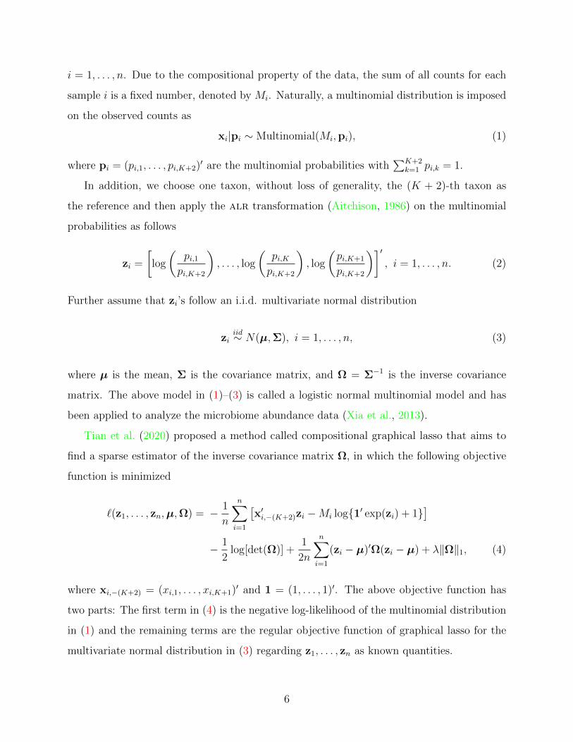
i = 1, . . . , n. Due to the compositional property of the data, the sum of all counts for each

sample i is a fixed number, denoted by Mi. Naturally, a multinomial distribution is imposed

on the observed counts as

xi|pi ∼ Multinomial(Mi,pi), (1)

where pi = (pi,1, . . . , pi,K+2)′ are the multinomial probabilities with

∑K+2k=1 pi,k = 1.

In addition, we choose one taxon, without loss of generality, the (K + 2)-th taxon as

the reference and then apply the alr transformation (Aitchison, 1986) on the multinomial

probabilities as follows

zi =

[log

(pi,1pi,K+2

), . . . , log

(pi,Kpi,K+2

), log

(pi,K+1

pi,K+2

)]′, i = 1, . . . , n. (2)

Further assume that zi’s follow an i.i.d. multivariate normal distribution

ziiid∼ N(µ,Σ), i = 1, . . . , n, (3)

where µ is the mean, Σ is the covariance matrix, and Ω = Σ−1 is the inverse covariance

matrix. The above model in (1)–(3) is called a logistic normal multinomial model and has

been applied to analyze the microbiome abundance data (Xia et al., 2013).

Tian et al. (2020) proposed a method called compositional graphical lasso that aims to

find a sparse estimator of the inverse covariance matrix Ω, in which the following objective

function is minimized

`(z1, . . . , zn,µ,Ω) = − 1

n

n∑i=1

[x′i,−(K+2)zi −Mi log1′ exp(zi) + 1

]− 1

2log[det(Ω)] +

1

2n

n∑i=1

(zi − µ)′Ω(zi − µ) + λ‖Ω‖1, (4)

where xi,−(K+2) = (xi,1, . . . , xi,K+1)′ and 1 = (1, . . . , 1)′. The above objective function has

two parts: The first term in (4) is the negative log-likelihood of the multinomial distribution

in (1) and the remaining terms are the regular objective function of graphical lasso for the

multivariate normal distribution in (3) regarding z1, . . . , zn as known quantities.

6

2.3 Reference-Invariant Objective Function

Similar to Section 2.1, if we choose another taxon, for simplicity of illustration, the (K+1)-th

taxon as the reference, then the alr transformation in (2) becomes

zi,p =

[log

(pi,1pi,K+1

), . . . , log

(pi,Kpi,K+1

), log

(pi,K+2

pi,K+1

)]′.

As in Sections 2.1, zi,p = Qpzi. Therefore, zi,piid∼ N(µp,Σp), i = 1, . . . , n, where µp = Qpµ,

Σp = QpΣQ′p, and Ωp = (Q′p)−1ΩQ−1p . The reference-invariance property in Section 2.1

implies that Ω1:K,1:K = Ωp,1:K,1:K .

The different choice of the reference also leads to a different objective function for the

compositional graphical lasso method (Comp-gLASSO) as follows

`p(z1,p, . . . , zn,p,µp,Ωp) = − 1

n

n∑i=1

[x′i,−(K+1)zi,p −Mi log1′ exp(zi,p) + 1

]− 1

2log[det(Ωp)] +

1

2n

n∑i=1

(zi,p − µp)′Ωp(zi,p − µp) + λ‖Ωp‖1,

(5)

where xi,−(K+1) = (xi,1, . . . , xi,K , xi,K+2)′ and 1 = (1, . . . , 1)′. Comparing (4) and (5),

their first terms are the same as they both equal to the negative log-likelihood of the

multinomial distribution: − 1n

∑ni=1

∑K+2k=1 xi,k log pi,k. In addition, from Aitchison (1986),

det(Ω) = det(Ωp) and∑n

i=1(zi − µ)′Ω(zi − µ) =∑n

i=1(zi,p − µp)′Ωp(zi,p − µp) as known

properties of the alr transformation. However, the L1 penalties in (4) and (5) are different

because Ω is not necessarily equal to Ωp. The reference-invariance property only implies

that Ω1:K,1:K = Ωp,1:K,1:K .

Motivated by the reference-invariance property, we can impose the L1 penalties only on

the invariant entries of Ω instead of all entries of Ω as in (4), which leads to

`inv(z1, . . . , zn,µ,Ω) = − 1

n

n∑i=1

[x′i,−(K+2)zi −Mi log1′ exp(zi) + 1

]− 1

2log[det(Ω)] +

1

2n

n∑i=1

(zi − µ)′Ω(zi − µ) + λ‖Ω1:K,1:K‖1. (6)

7

With the previous arguments, we showed that `inv(z1, . . . , zn,µ,Ω) is reference-invariant; in

other words, the objective function `inv stays the same regardless of whether the (K + 1)-th

or the (K + 2)-th taxa is selected as the reference. This is summarized in the following

theorem.

Theorem 2. If zi,p = Qpzi for i = 1, . . . , n, µp = Qpµ, and Ωp = (Q′p)−1ΩQ−1p , then

`inv(z1, . . . , zn,µ,Ω) = `inv,p(z1,p, . . . , zn,p,µp,Ωp).

We call `inv(z1, . . . , zn,µ,Ω) in (6) the reference-invariant compositional graphical lasso

objective function. The invariance of the objective function also implies the invariance of its

minimizer. We call the minimizer Ω of (6) the reference-invariant compositional graphical

lasso (Inv-Comp-gLASSO) solution.

In general, suppose we have selected a set of taxa xR as “candidate references” and write

x = (x′Rc ,x′R)′. Then, the reference-invariant objective function becomes

`inv(z1, . . . , zn,µ,Ω) = − 1

n

n∑i=1

[x′i,−(K+2)zi −Mi log1′ exp(zi) + 1

]− 1

2log[det(Ω)] +

1

2n

n∑i=1

(zi − µ)′Ω(zi − µ) + λ‖ΩRc,Rc‖1. (7)

In other words, (7) is invariant regardless of which reference is selected in the set of candidate

references, and so is its minimizer.

It is noteworthy that the trick we played in defining the reference-invariant version of

Comp-gLASSO is to revise the penalty term from the regular lasso penalty on the whole

inversion covariance matrix to that only on the invariant part of the inversion covariance

matrix. Using the same trick, we can define the reference-invariant version of other methods

such as reference-invariant graphical lasso (Inv-gLASSO). The objective function of Inv-

gLASSO is defined as follows when z1, . . . , zn are observed instead of x1, . . . ,xn:

`inv(µ,Ω) = −1

2log[det(Ω)] +

1

2n

n∑i=1

(zi − µ)′Ω(zi − µ) + λ‖ΩRc,Rc‖1. (8)

The objective function (8) includes naturally three sets of parameters (z1, . . . , zn), µ, and

Ω, which motivates us to apply a block coordinate descent algorithm. A block coordinate

8

descent algorithm minimizes the objective function iteratively for each set of parameters

given the other sets. Given the initial values (z(0)1 , . . . , z

(0)n ), µ(0), and Ω(0), a block coordinate

algorithm repeats the following steps cyclically for iteration t = 0, 1, 2, . . . until the algorithm

converges.

1. Given µ(t) and Ω(t), find (z(t+1)1 , . . . , z

(t+1)n ) that maximizes (8).

2. Given (z(t+1)1 , . . . , z

(t+1)n ) and Ω(t), find µ(t+1) that maximizes (8).

3. Given (z(t+1)1 , . . . , z

(t+1)n ) and µ(t+1), find Ω(t+1) that maximizes (8).

Except for the mild modification on the objective function, the details of the algorithm

is essentially the same as the one described in Tian et al. (2020).

3 Simulation Study

3.1 Settings

To illustrate the reference-invariance property under the aforementioned framework, we con-

duct a simulation study and evaluated the performance of Inv-Comp-gLASSO as well as

Inv-gLASSO.

Following Tian et al. (2020), we generated three types of inverse covariance matrices

Ω = (ωkl)1≤k,l≤K+1 as follows:

1. Chain: ωkk = 1.5, ωkl = 0.5 if |k − l| = 1, and Ωkl = 0 if |k − l| > 1. Every node is

connected to the adjacent node, and therefore the connectedness is 1 for all but two

nodes.

2. Random: ωkl = 1 with probability 3/(K+1) for k 6= l. Every two nodes are connected

with a fixed probability, and the expected connected is the same for all nodes.

3. Hub: Nodes are randomly partitioned into d(K+ 1)/20e groups, and there’s one “hub

node” in each group. For the other nodes in the group, they are only connected to

the hub node but not each other. There’s no connection among groups. The degree of

connectedness is much higher for the hub nodes (24), and is 1 for the rest of the nodes.

9

In the simulations, we also varied two other factors that play a crucial role in the perfor-

mances of the methods:

1. Sequencing depth. Mi’s are simulated from Uniform(20K, 40K) or Uniform(100K, 200K),

denoted by “low” and “high” sequencing depth.

2. Compositional variation. For each aforementioned inverse covariance matrix Ω

(“low” compositional variation), we also divide each of them by a factor of 5 to obtain

another set of inverse covariance matrices, i.e., Ω/5 (“high” compositional variation).

The data are simulated from the logistic normal multinomial distribution in (1)–(3). In

detail, zi ∼ N(µ,Σ) were first generated independently for i = 1, . . . , n; then, the softmax

transformation (the inverse of the alr transformation) was applied to get the multinomial

probabilities pi with the (K+2)-th entry serving as the true reference; last, the multinomial

random variables xi were simulated from Multinomial(Mi; pi), for i = 1, . . . , n. We set

n = 100 and K = 49 throughout the simulations.

The simulation results are based on 100 replicates of the simulated data. Both Inv-Comp-

gLASSO and Inv-gLASSO were applied with two choices of reference, the (K + 1)-th entry

serving as the false reference and the (K+2)-th entry serving as the true reference. and only

the reference-invariant sub-network Ω1:K,1:K is used in the evaluations. For Inv-gLASSO, we

estimated p1, . . . ,pn with x1/M1, . . . ,xn/Mn, and performed the alr transformation to get

the estimates of z1, . . . , zn, which were denoted by z1, . . . , zn. We then apply Inv-gLASSO to

z1, . . . , zn directly to find the inverse covariance matrix Ω, which also serves as the starting

value for Inv-Comp-gLASSO. For both methods, we implemented them with a common

sequence of 70 tuning parameters of λ.

We empirically validate the invariance property of Inv-Comp-gLASSO and Inv-gLASSO

by comparing the estimators of the two sub-networks Ω1:K,1:K resulted from choosing the

true and false reference separately in each method, which have been shown to be theoretically

invariant in Section 2. The comparison is assessed under four criteria as follows.

1. Normalized Manhattan Similarity

10

For two matrices A and B, we define the normalized Manhattan similarity (NMS) as

NMS(A,B) = 1− ‖A−B‖1‖A‖1 + ‖B‖1

,

where ‖·‖1 represents the entrywise L1 norm of a matrix. Note that 0 ≤ NMS ≤ 1 due

to the non-negativity of norms and the triangle inequality.

2. Jaccard Index

For two networks with the same nodes, denote their set of edges by A and B. Then

the Jaccard Index (Jaccard, 1901) is defined as follows:

J(A,B) =|A ∩ B||A ∪ B|

.

Obviously, it also holds that 0 ≤ J(A,B) ≤ 1.

3. Normalized Hamming Similarity

In the context of network comparison, the normalized Hamming similarity for two

adjacency matrices A and B with the same N nodes are defined as follows (Hamming,

1950)

H(A,B) = 1− ‖A−B‖1N(N − 1)

,

where ‖·‖1 denotes the entrywise L1 norm of a matrix. Since there are at most N(N−1)

edges in a network with N nodes, this metric is also between 0 and 1.

4. ROC Curve

The ROC curves on which true positive rate (TPR) and false positive rate (FPR) are

plotted are also compared between the choices of true and false reference.

3.2 Results

3.2.1 Normalized Manhattan Similarity

The normalized Manhattan similarity serves as a direct measure of the similarity between

the two estimated inverse covariance matrices with different choices of the reference. On

11

a sequence of 70 tuning parameter λ’s, we calculated the normalized Manhattan similarity

between the two estimated inverse covariance matrices with the true and false references

separately. Figure 1 shows the average normalized Manhattan similarity over 100 replicates

along with standard error bars.

Chain

0.0

0.1

0.2

0.3

0.4

0.5

0.6

0.7

0.8

0.9

1.0

λ (Decreasing)

h, h

0.0

0.1

0.2

0.3

0.4

0.5

0.6

0.7

0.8

0.9

1.0

λ (Decreasing)

h, l

0.0

0.1

0.2

0.3

0.4

0.5

0.6

0.7

0.8

0.9

1.0

λ (Decreasing)

l, h

0.0

0.1

0.2

0.3

0.4

0.5

0.6

0.7

0.8

0.9

1.0

λ (Decreasing)

l, l

Random

0.0

0.1

0.2

0.3

0.4

0.5

0.6

0.7

0.8

0.9

1.0

λ (Decreasing)

h, h

0.0

0.1

0.2

0.3

0.4

0.5

0.6

0.7

0.8

0.9

1.0

λ (Decreasing)

h, l

0.0

0.1

0.2

0.3

0.4

0.5

0.6

0.7

0.8

0.9

1.0

λ (Decreasing)

l, h

0.0

0.1

0.2

0.3

0.4

0.5

0.6

0.7

0.8

0.9

1.0

λ (Decreasing)

l, l

Hub

0.0

0.1

0.2

0.3

0.4

0.5

0.6

0.7

0.8

0.9

1.0

λ (Decreasing)

h, h

0.0

0.1

0.2

0.3

0.4

0.5

0.6

0.7

0.8

0.9

1.0

λ (Decreasing)

h, l

0.0

0.1

0.2

0.3

0.4

0.5

0.6

0.7

0.8

0.9

1.0

λ (Decreasing)

l, h

0.0

0.1

0.2

0.3

0.4

0.5

0.6

0.7

0.8

0.9

1.0

λ (Decreasing)

l, l

Nor

mal

ized

Man

hatta

n S

imila

rity

Figure 1: Normalized Manhattan similarity between the two estimated inverse covariancematrices with true and false references. Solid: Inv-Comp-gLASSO; dashed: Inv-gLASSO.h,h: high sequencing depth, high compositional variation; h, l: high sequencing depth, lowcompositional variation; l,h: low sequencing depth, high compositional variation; l, l: lowsequencing depth, low compositional variation.

We can see from Figure 1 that, the normalized Manhattan similarity for Inv-gLASSO

stays close to 1 in all settings, throughout the whole sequence of tuning parameters. On

the other hand, there are some fluctuations in the same metric from Inv-Comp-gLASSO,

12

although most values stay higher than 0.9. Empirically, the two estimated matrices are nu-

merically identical for Inv-gLASSO and close for Inv-Comp-gLASSO. A potential reason why

the invariance of Inv-gLASSO is numerically more evident than that of Inv-Comp-gLASSO

is that Inv-gLASSO is a convex optimization while Inv-Comp-gLASSO is not necessarily

convex (Tian et al., 2020). With different starting points (as we choose different references),

Inv-Comp-gLASSO might result in different solutions as the algorithm is only guaranteed to

converge to a stationary point. We refer to Tian et al. (2020) for more detailed discussion

about the convexity and convergences of the algorithm.

In addition, it is consistently observed that the normalized Manhattan similarity for Inv-

Comp-gLASSO starts close to 1 when λ is very large and gradually decreases with some

fluctuations as λ decreases. This is because the Inv-Comp-gLASSO objective function in (6)

is solved by an iterative algorithm between graphical lasso to estimate (µ,Ω) and Newton-

Raphson to estimate z1, . . . , zn, which can lead to more numerical errors depending on the

number of iterations. Furthermore, the algorithm is implemented with warm start for a

sequence of decreasing λ’s, i.e., the solution for the previous λ value is used as the starting

point for the current λ value. With the accumulation of numerical errors, the numerical

difference between the two estimated matrices becomes larger.

Among the simulation settings, we find the invariance property for Inv-Comp-gLASSO is

most evidently supported by the numerical results in the “high sequencing depth, low com-

positional variation” setting, regardless of the network types. The normalized Manhattan

similarity is very close to 1 for Inv-Comp-gLASSO throughout the sequence of tuning pa-

rameters. This is because the compositional probabilities pi’s and thus the zi’s are estimated

accurately with high sequencing depth and low compositional variation in the first iteration

of the Inv-Comp-gLASSO algorithm, which implies fewer iterations for the algorithm to

converge and less numeric error accumulated during this process. On the other hand, the

normalized Manhattan similarity is the lowest in the “low sequencing depth, high composi-

tional variation” setting. It is due to a similar reason that it takes more iterations for the

Inv-Comp-gLASSO algorithm to converge, accumulating more numerical errors. However,

it is noteworthy that this is exactly the setting in which Inv-Comp-gLASSO has the most

advantage over Inv-gLASSO in recovering the true network (see Section 3.2.3 for their ROC

13

curves).

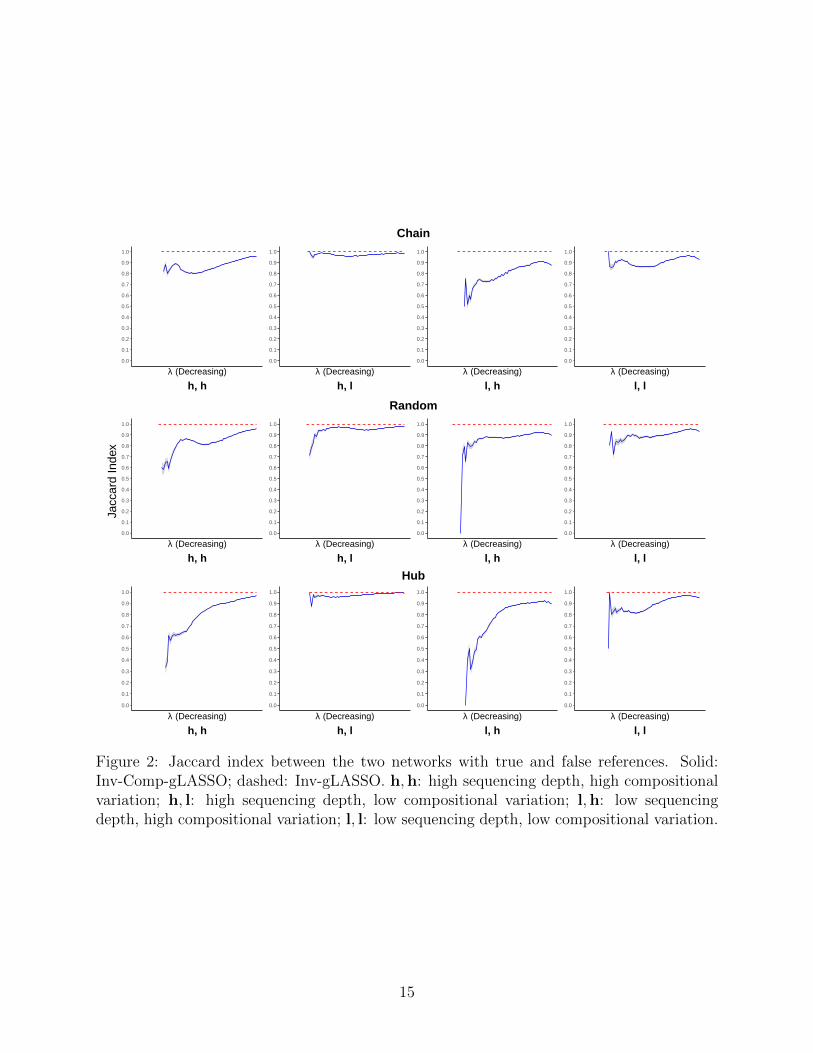
3.2.2 Jaccard Index and Normalized Hamming Similarity

Compared to normalized Manhattan similarity that measures directly the similarity between

two inverse covariane matrices, both Jaccard index and normalized Hamming similarity

measure the similarity between two networks represented by the matrices because they only

compared the adjacency matrices or the edges of the two networks. Again, on a sequence

of 70 tuning parameter λ’s, we computed the Jaccard index and the normalized Hamming

similarity between the two networks with true and false references separately. Figures 2 and

3 plot the average Jaccard index and the normalized Hamming similarity over 100 replicates

along with standard error bars.

The results of normalized Hamming similarity in Figure 3 have a fairly similar pattern to

those of normalized Manhattan similarity in Figure 1 and thus can be similarly interpreted.

We only focus on the results of Jaccard index in Figure 2 here. The Jaccard index stays close

to 1 for Inv-gLASSO, implying the identity between the two networks. Although the results

of the Jaccard index for Inv-Comp-gLASSO look quite different from the other measures at

the first glance, it actually implies a similar conclusion. First, we notice that there is no

Jaccard index for the first few tuning parameters that are large enough. This is because the

resultant network is empty with either true or false reference. Although two empty networks

agree with each other perfectly, the Jaccard index is not well defined. Then, as Inv-Comp-

gLASSO starts to pick up edges when lambda decreases, the Jaccard index is quite low

in some settings, suggesting that the two networks are dissimilar. However, this is due to

the fact the Jaccard index is a much more “strict” similarity measure than the Hamming

similarity. For example, for two networks with 100 possible total edges, if both networks only

have one but a different edge, then the Jaccard index is 0 while the normalized Hamming

similarity is 0.98. Finally, as the networks become denser, the Jaccard index increases quickly

and stabilizes at a quite high value in most settings.

It is also notable that both the Jaccard index and the normalized Hamming similarity

are relatively high in the “high sequencing depth, low compositional variation” setting and

relatively low in the “low sequencing depth, high compositional variation” setting, which is

14

Chain

0.0

0.1

0.2

0.3

0.4

0.5

0.6

0.7

0.8

0.9

1.0

λ (Decreasing)

h, h

0.0

0.1

0.2

0.3

0.4

0.5

0.6

0.7

0.8

0.9

1.0

λ (Decreasing)

h, l

0.0

0.1

0.2

0.3

0.4

0.5

0.6

0.7

0.8

0.9

1.0

λ (Decreasing)

l, h

0.0

0.1

0.2

0.3

0.4

0.5

0.6

0.7

0.8

0.9

1.0

λ (Decreasing)

l, l

Random

0.0

0.1

0.2

0.3

0.4

0.5

0.6

0.7

0.8

0.9

1.0

λ (Decreasing)

h, h

0.0

0.1

0.2

0.3

0.4

0.5

0.6

0.7

0.8

0.9

1.0

λ (Decreasing)

h, l

0.0

0.1

0.2

0.3

0.4

0.5

0.6

0.7

0.8

0.9

1.0

λ (Decreasing)

l, h

0.0

0.1

0.2

0.3

0.4

0.5

0.6

0.7

0.8

0.9

1.0

λ (Decreasing)

l, l

Hub

0.0

0.1

0.2

0.3

0.4

0.5

0.6

0.7

0.8

0.9

1.0

λ (Decreasing)

h, h

0.0

0.1

0.2

0.3

0.4

0.5

0.6

0.7

0.8

0.9

1.0

λ (Decreasing)

h, l

0.0

0.1

0.2

0.3

0.4

0.5

0.6

0.7

0.8

0.9

1.0

λ (Decreasing)

l, h

0.0

0.1

0.2

0.3

0.4

0.5

0.6

0.7

0.8

0.9

1.0

λ (Decreasing)

l, l

Jacc

ard

Inde

x

Figure 2: Jaccard index between the two networks with true and false references. Solid:Inv-Comp-gLASSO; dashed: Inv-gLASSO. h,h: high sequencing depth, high compositionalvariation; h, l: high sequencing depth, low compositional variation; l,h: low sequencingdepth, high compositional variation; l, l: low sequencing depth, low compositional variation.

15

Chain

0.0

0.1

0.2

0.3

0.4

0.5

0.6

0.7

0.8

0.9

1.0

λ (Decreasing)

h, h

0.0

0.1

0.2

0.3

0.4

0.5

0.6

0.7

0.8

0.9

1.0

λ (Decreasing)

h, l

0.0

0.1

0.2

0.3

0.4

0.5

0.6

0.7

0.8

0.9

1.0

λ (Decreasing)

l, h

0.0

0.1

0.2

0.3

0.4

0.5

0.6

0.7

0.8

0.9

1.0

λ (Decreasing)

l, l

Random

0.0

0.1

0.2

0.3

0.4

0.5

0.6

0.7

0.8

0.9

1.0

λ (Decreasing)

h, h

0.0

0.1

0.2

0.3

0.4

0.5

0.6

0.7

0.8

0.9

1.0

λ (Decreasing)

h, l

0.0

0.1

0.2

0.3

0.4

0.5

0.6

0.7

0.8

0.9

1.0

λ (Decreasing)

l, h

0.0

0.1

0.2

0.3

0.4

0.5

0.6

0.7

0.8

0.9

1.0

λ (Decreasing)

l, l

Hub

0.0

0.1

0.2

0.3

0.4

0.5

0.6

0.7

0.8

0.9

1.0

λ (Decreasing)

h, h

0.0

0.1

0.2

0.3

0.4

0.5

0.6

0.7

0.8

0.9

1.0

λ (Decreasing)

h, l

0.0

0.1

0.2

0.3

0.4

0.5

0.6

0.7

0.8

0.9

1.0

λ (Decreasing)

l, h

0.0

0.1

0.2

0.3

0.4

0.5

0.6

0.7

0.8

0.9

1.0

λ (Decreasing)

l, l

Nor

mal

ized

Ham

min

g S

imila

rity

Figure 3: Normalized Hamming similarity between the two networks with true and false ref-erences. Solid: Inv-Comp-gLASSO; dashed: Inv-gLASSO. h,h: high sequencing depth, highcompositional variation; h, l: high sequencing depth, low compositional variation; l,h: lowsequencing depth, high compositional variation; l, l: low sequencing depth, low compositionalvariation.

16

consistent with the finding for the normalized Manhattan similarity.

3.2.3 ROC Curves

An ROC curve is plotted from the average of true positive rates and the average of false

positive rates over 100 replicates. An ROC curve can be regarded as an indirect measure of

the invariance (two networks possessing similar ROC curves is a necessary but not sufficient

condition for the two networks are similar). However, it is crucial to evaluate the algorithms

with this criterion, since it answers the question: “Does the performance of the algorithm

depends on the choice of reference?”

We could see that the ROC curves from Inv-Comp-gLASSO, regardless of the choice of

the reference, dominate the ones from Inv-gLASSO in all settings. The two ROC curves

from Inv-gLASSO lay perfectly on top of each other, while the curves from Inv-Comp-

gLASSO are also fairly close to each other. These empirical results validate the theoretical

reference-invariance property for both methods. In addition, Inv-Comp-gLASSO has the

most obvious advantage over Inv-gLASSO in the “low sequencing depth, high compositional

variation” setting and they perform almost identically in the “low sequencing depth, high

compositional variation” setting. Although the similarity measures are lower in the “most

favorable” setting for Inv-Comp-gLASSO (see Sections 3.2.1 and 3.2.2), the ROC curves of

the two networks from the method do not deviate too much from each other in this setting.

4 Real Data

To further validate the theoretical reference-invariance properties of Inv-Comp-gLASSO and

Inv-gLASSO, we applied them to a dataset from the TARA Ocean project, in which the

Tara Oceans consortium sampled both plankton and environmental data in 210 sites from

the world oceans. The data collected was later analyzed using sequencing and imaging tech-

niques. We downloaded the taxonomic data and the literature interactions from the TARA

Ocean Project data repository (https://doi.pangaea.de/10.1594/PANGAEA.843018). As

part of the TARA Oceans project, Lima-Mendez et al. (2015) investigated the impact of both

biotic and abiotic interactions in oceanic ecosystem. In this article, a literature-curated list

17

Chain

0.00

0.25

0.50

0.75

1.00

0.00 0.25 0.50 0.75 1.00

FP

TP

h, h

0.00

0.25

0.50

0.75

1.00

0.00 0.25 0.50 0.75 1.00

FP

TP

h, l

0.00

0.25

0.50

0.75

1.00

0.00 0.25 0.50 0.75 1.00

FP

TP

l, h

0.00

0.25

0.50

0.75

1.00

0.00 0.25 0.50 0.75 1.00

FP

TP

l, l

Random

0.00

0.25

0.50

0.75

1.00

0.00 0.25 0.50 0.75 1.00

FP

TP

h, h

0.00

0.25

0.50

0.75

1.00

0.00 0.25 0.50 0.75 1.00

FP

TP

h, l

0.00

0.25

0.50

0.75

1.00

0.00 0.25 0.50 0.75 1.00

FPT

P

l, h

0.00

0.25

0.50

0.75

1.00

0.00 0.25 0.50 0.75 1.00

FP

TP

l, l

Hub

0.00

0.25

0.50

0.75

1.00

0.00 0.25 0.50 0.75 1.00

FP

TP

h, h

0.00

0.25

0.50

0.75

1.00

0.00 0.25 0.50 0.75 1.00

FP

TP

h, l

0.00

0.25

0.50

0.75

1.00

0.00 0.25 0.50 0.75 1.00

FP

TP

l, h

0.00

0.25

0.50

0.75

1.00

0.00 0.25 0.50 0.75 1.00

FP

TP

l, l

Figure 4: ROC curves for Inv-Comp-gLASSO and Inv-gLASSO with true and false references.Solid blue: Inv-Comp-gLASSO with true reference; dashed red: Inv-Comp-gLASSO withfalse reference; dashed dotted blue: Comp-gLASSO with true reference; dotted red: Comp-gLASSO with false reference. h,h: high sequencing depth and high compositional variation;h, l: high sequencing depth and low compositional variation; l,h: low sequencing depth andhigh compositional variation; l, l: low sequencing depth and low compositional variation.

of genus-level marine eukaryotic plankton interactions was generated by a panel of experts.

Similar to Tian et al. (2020), we focused the analysis on genus level and only kept the

81 genus involved in the literature-reported interactions. For computational simplicity, we

removed the samples with too small reads (< 100). As a result, it leaves with 324 samples

in the final preprocessed data. From the genera that were not reported in the literature, we

chose two of them, Acrosphaera and Collosphaera, with the largest average relative abun-

18

dances as the references. We then applied both Inv-Comp-gLASSO and Inv-gLASSO to the

textscalr-transformed data with those two references, with a common sequence of tuning

parameters. For each combination of a method and a reference, we also selected a tuning

parameter that corresponds to the “asymptotically sparsistent” (the sparsest estimated net-

work in the path that contains the true network with a high probability) network by StARS

(Liu et al., 2010).

selected by StARS

0.0

0.1

0.2

0.3

0.4

0.5

0.6

0.7

0.8

0.9

1.0

λ (Decreasing)

Nor

mal

ized

Mah

atta

n S

imila

rity

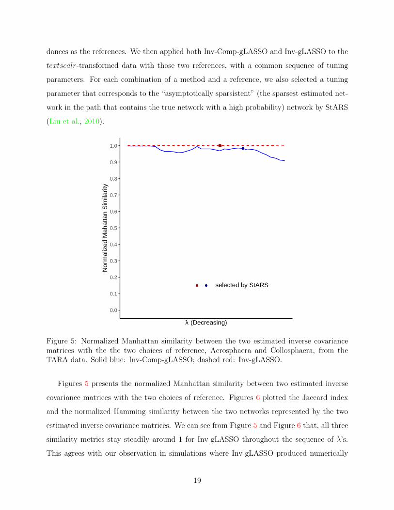
Figure 5: Normalized Manhattan similarity between the two estimated inverse covariancematrices with the the two choices of reference, Acrosphaera and Collosphaera, from theTARA data. Solid blue: Inv-Comp-gLASSO; dashed red: Inv-gLASSO.

Figures 5 presents the normalized Manhattan similarity between two estimated inverse

covariance matrices with the two choices of reference. Figures 6 plotted the Jaccard index

and the normalized Hamming similarity between the two networks represented by the two

estimated inverse covariance matrices. We can see from Figure 5 and Figure 6 that, all three

similarity metrics stay steadily around 1 for Inv-gLASSO throughout the sequence of λ’s.

This agrees with our observation in simulations where Inv-gLASSO produced numerically

19

selected by StARS

0.00

0.25

0.50

0.75

1.00

λ (Decreasing)

Jacc

ard

Inde

x

selected by StARS

0.0

0.1

0.2

0.3

0.4

0.5

0.6

0.7

0.8

0.9

1.0

λ (Decreasing)N

orm

aliz

ed H

amm

ing

Sim

ilarit

y

Figure 6: Jaccard index and normalized Hamming similarity between the two estimatednetworks with the the two choices of reference, Acrosphaera and Collosphaera, from theTARA data. Solid blue: Inv-Comp-gLASSO; dashed red: Inv-gLASSO.

identical inverse covariance matrices.

For Inv-Comp-gLASSO, the similarity scores start around 1 (for normalized Manhattan

similarity and normalized Hamming similarity) or non-existent (for Jaccard index) when

the estimated networks are empty. Then, as λ decreases, the estimated networks become

denser, and the measures start to fluctuate and decline slightly at the end. In spite of

the fluctuations, both normalized Manhattan similarity and normalized Hamming similarity

stay above 0.9, while the lowest Jaccard index is about 0.64. As discussed earlier, Jaccard

index is a stricter measure than normalized Manhattan similarity and normalized Hamming

similarity.

With each method, StARS picked the same tuning parameter λ regardless of the choice

of the reference, as denoted by the red dot for Inv-gLASSO and the blue dot for Inv-Comp-

gLASSO in Figures 5 and 6. In other words, the red and blue dots represent the tuning

parameters corresponding to the final estimated networks selected by StARS. Again, the

three similarity measures for the two final inverse covariance matrices or networks from

Inv-gLASSO is almost 1, while the normalized Manhattan similarity, Jaccard index, and

20

normalized Hamming similarity are 0.98, 0.96 and 0.99 for Inv-Comp-gLASSO. All these high

similarity scores imply the empirical invariance for Inv-gLASSO and Inv-Comp-gLASSO.

Both methods result in invariant inverse covariance matrices and thus the corresponding

networks with respect to the choices of the reference genus (Acrosphaera or Collosphaera)

when applied to the TARA Ocean eukaryotic dataset.

5 Discussion

In this work, we established the reference-invariance property in sparse inverse covariance

matrix estimation and network construction based on the alr transformed data. Then, we

proposed the reference-invariant versions of the compositional graphical lasso and graphical

lasso by modifying the penalty in their respective objective functions. In addition, we val-

idated the reference-invariance property of the proposed methods empirically by applying

them to various scenarios of simulations and a real TARA Ocean eukaryotic dataset.

It is noteworthy that the reference-invariance property is a general property for esti-

mating the inverse covariance matrix based on the alr transformed data. We proposed

reference-invariant versions of compositional graphical lasso and graphical lasso based on

this property, however, one may revise other existing methods for inverse covariance matrix

estimation based on the alr transformed data. The trick is to revise the objective function

so that it becomes invariant with respect to the choice of the reference. Subsequently, the

resultant inverse covariance matrix and network are expected to be reference-invariant both

theoretically and empirically, the latter of which may depend on the algorithm that is used

to optimize the reference-invariant objective function.

References

Aitchison, J. (1986), The statistical analysis of compositional data, Monographs on statistics

and applied probability, Chapman and Hall.

Arrigo, K. R. (2004), “Marine microorganisms and global nutrient cycles,” Nature, 437, 349.

21

Ban, Y., An, L., and Jiang, H. (2015), “Investigating microbial co-occurrence patterns based

on metagenomic compositional data,” Bioinformatics, 31, 3322–3329.

Fang, H., Huang, C., Zhao, H., and Deng, M. (2015), “CCLasso: correlation inference for

compositional data through Lasso,” Bioinformatics, 31, 3172–3180.

— (2017), “gCoda: conditional dependence network inference for compositional data,” Jour-

nal of Computational Biology, 24, 699–708.

Faust, K. and Raes, J. (2012), “Microbial interactions: from networks to models,” Nature

Reviews Microbiology, 10, 538.

Friedman, J. and Alm, E. J. (2012), “Inferring correlation networks from genomic survey

data,” PLoS computational biology, 8, e1002687.

Friedman, J., Hastie, T., and Tibshirani, R. (2008), “Sparse inverse covariance estimation

with the graphical lasso,” Biostatistics, 9, 432–441.

Hamming, R. W. (1950), “Error detecting and error correcting codes,” The Bell system

technical journal, 29, 147–160.

Jaccard, P. (1901), “Distribution de la flore alpine dans le bassin des Dranses et dans quelques

regions voisines,” Bull Soc Vaudoise Sci Nat, 37, 241–272.

Jiang, D., Sharpton, T., and Jiang, Y. (2020), “Microbial Interaction Network Estimation

via Bias-Corrected Graphical Lasso,” To appear.

Kamada, N., Chen, G. Y., Inohara, N., and Nunez, G. (2013), “Control of pathogens and

pathobionts by the gut microbiota,” Nature immunology, 14, 685.

Kohl, K. D., Weiss, R. B., Cox, J., Dale, C., and Denise Dearing, M. (2014), “Gut microbes

of mammalian herbivores facilitate intake of plant toxins,” Ecology letters, 17, 1238–1246.

Kurtz, Z. D., Muller, C. L., Miraldi, E. R., Littman, D. R., Blaser, M. J., and Bonneau, R. A.

(2015), “Sparse and compositionally robust inference of microbial ecological networks,”

PLoS computational biology, 11, e1004226.

22

Lima-Mendez, G., Faust, K., Henry, N., Decelle, J., Colin, S., Carcillo, F., Chaffron, S.,

Ignacio-Espinosa, J. C., Roux, S., Vincent, F., et al. (2015), “Determinants of community

structure in the global plankton interactome,” Science, 348, 1262073.

Liu, H., Roeder, K., and Wasserman, L. (2010), “Stability approach to regularization se-

lection (stars) for high dimensional graphical models,” in Advances in neural information

processing systems, pp. 1432–1440.

Mazmanian, S. K., Round, J. L., and Kasper, D. L. (2008), “A microbial symbiosis factor

prevents intestinal inflammatory disease,” Nature, 453, 620.

Tian, C., Jiang, D., and Jiang, Y. (2020), “Microbial Network Recovery by Compositional

Graphical Lasso,” Manuscript in preparation.

Xia, F., Chen, J., Fung, W. K., and Li, H. (2013), “A logistic normal multinomial regression

model for microbiome compositional data analysis,” Biometrics, 69, 1053–1063.

Yuan, H., He, S., and Deng, M. (2019), “Compositional data network analysis via lasso

penalized D-trace loss,” Bioinformatics, 35, 3404–3411.

Yuan, M. and Lin, Y. (2007), “Model selection and estimation in the Gaussian graphical

model,” Biometrika, 94, 19–35.

23